estudos econômicos (são paulo) this is an open access

Estudos Econômicos (São Paulo) This is an Open Access artcle distributed under the terms of the Creatie Commons

Attributon NoniCommercial License which permits unrestricted nonicommercial usec distributoncand reproducton in any medium proiided the original work is properly cited. Fonte:http://www.scielo.br/scielo.phpsscriptssciaarttext&pidsS1010i40602107111211295&lngsen&nrmsiso. Acesso em: 21 fei. 2108.

REFERÊNCIACOSTA FILHOc Adonias Eiaristo da. Monetary policy in Brazil: eiidence from new measures of monetary shocks. Estudos Econômicos (São Paulo)c São Pauloc i. 47c n. 2c p. 295i328c abr./jun. 2107. Disponíiel em: <http://www.scielo.br/scielo.phpsscriptssciaarttext&pidsS1010i40602107111211295&lngsen&nrmsiso>. Acesso em: 21 fei. 2108. doi: http://dx.doi.org/01.0591/1010i406047232aecf.

http://creativecommons.org/licenses/by-nc/4.0/deed.en

Estud. Econ., São Paulo, vol.47, n.2, p.295-328, abr.-jun. 2017

DOI: http://dx.doi.org/10.1590/0101-416147232aecf

Monetary policy in Brazil: Evidence from new measures of monetary shocks ♦

Adonias Evaristo da Costa FilhoDoutor em Economia – Universidade de Brasília (UnB)E-mail: [email protected]

Recebido: 08/04/2016. Aceite: 19/12/2016.

AbstractThis paper derives new measures of monetary policy shocks for Brazil. First, one set of shocks is built inspired by Romer and Romer (2004) methodology, using official and private forecasts. Central Bank staff forecasts were collected from the technical presentations of monetary policy meetings, released after the introduction of the Access of Information Law, while private forecasts come from the Focus survey. Second, a yield curve shock is constructed for the Brazilian case, based on the Barakchian and Crowe (2013) methodology. Equipped with the shocks measu-res, I include them on VARs (Vector Autoregressions) and analyze the effects on inflation and output. A standardized monetary policy shock is found to reduce real GDP in up to 0.5%. In all but the yield curve shock case, it is found evidence of a price puzzle in the estimated models.

KeywordsMonetary policy. Shocks. Output. Inflation.

ResumoEste artigo deriva novas medidas de choques de política monetária para o Brasil. Em primeiro lugar, um conjunto de choques é construído inspirado na metodologia de Romer e Romer (2004), utilizando tanto previsões públicas quanto privadas. As previsões do Banco Central foram coletadas a partir das apresentações técnicas das reuniões de política monetária, que vêm se tornando públicas após a Lei de Acesso à Informação, enquanto as previsões do setor privado vêm da pesquisa Focus. Em segundo lugar, uma série de choque na curva de juros foi construída para o Brasil, baseada na metodologia de Barakchian and Crowe (2013). De posse das medidas de choques, foram estimados VARs (Vetores Autorregressivos), e analisados os efeitos na inflação e no produto. Encontra-se que um choque padronizado de política monetária reduz o PIB real em até 0,5%. Exceto para o caso do choque na curva de juros, para os demais casos são encontradas evidências de um “price puzzle” nos modelos estimados.

Palavras-ChavePolítica monetária. Choques. Produto. Inflação. Monetary policy. Shocks. Output. Inflation.

Classificação JEL E31. E32. E52. E58.

♦ As opiniões expressas no artigo são exclusivamente do autor.


296 Adonias Evaristo da Costa Filho

1. Introduction

This paper derives new measures of monetary policy shocks for Brazil, aiming to shed light on the effects of monetary policy on the Brazilian economy. Recently, there has been a renewed effort to analyze the ef-fects of monetary policy shocks, with some authors trying to reconcile the evidence (Coibon, 2012) or obtaining new measures of monetary policy shocks, as shown in the studies of Barakchian and Crowe (2013) for the United States and Cloyne and Hurtgen (2014) for the UK.

Following the approach of the aforementioned articles, this research em-ploys a comprehensive view of monetary policy shocks, investigating the effects on GDP and inflation of a total of three measures of shocks. Two shocks are derived in the spirit of the narrative approach introduced by Romer and Romer (RR) (2004). This method of obtaining monetary po-licy shocks consists in a regression of the change in the policy rate on the forecasts of inflation and GDP growth. The residuals from this regression are taken as the measure of monetary policy shocks. By using forecasts to estimate the effects of monetary policy, the methodology pursued here bears a strong resemblance to the one undertook by Thapar (2008), who used Federal Reserve’s Greenbook forecasts and expectations embedded in financial contracts to analyze the effects of monetary policy for the US economy. Brissimis and Magginas (2006) also argue for the use of ex-pectations variables to take into account the forward-looking behavior of central banks, including an index of leading indicators and federal funds futures in their models.

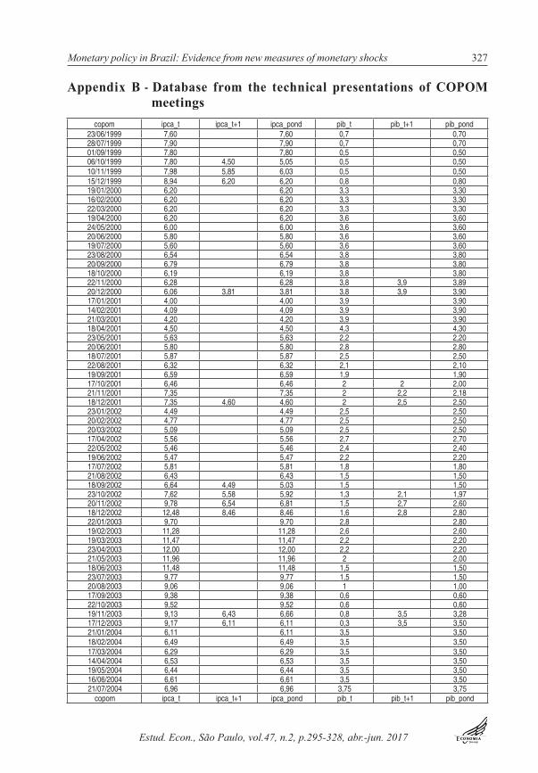
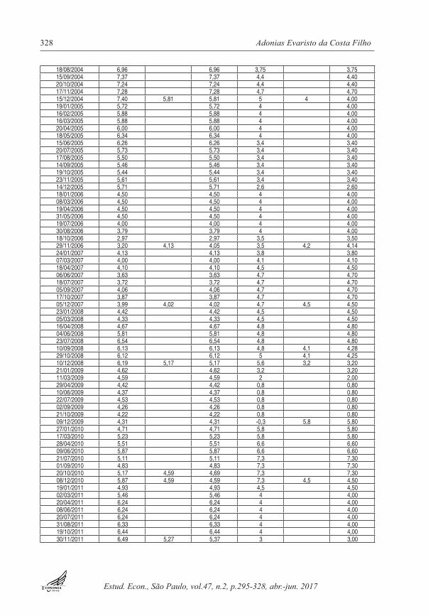
For the Brazilian case, the forecasts were collected from different sources. Both official and private forecasts were used. The official forecasts data come from the presentations of the Central Bank staff for the monetary policy committee (COPOM) meetings. These presentations became avai-lable after the Access of Information Law1 was introduced in 2011, which required that the content of the technical presentations of the first day of COPOM meetings would be available to the public after four years the meeting took place. Using these presentations, it was possible to build a new dataset of forecasts of GDP and inflation from the Central Bank staff at the time of each meeting.2 As of 2016, the presentations of COPOM 1 Law no 12.527 of 2011, “Lei de Acesso à Informação”, in Portuguese. 2 For GDP, the data collected usually appear on the slide “PIB” on section “Nível de Atividade”, and

corresponds to the estimated figure for the end of the 4th quarter of each year. For IPCA, the figures collected appear on section “Preços”, and correspond to the end of the year value on the slide “Esti-mativa de Inflação – IPCA-DEPEC”.

Monetary policy in Brazil: Evidence from new measures of monetary shocks 297


meetings from 1999 to 2011 were available. Due to the period required for disclosure by the law–4 years– it was not possible to obtain data for the more recent years. The database is presented in the Appendix. On the other hand, private forecasts came from the Focus survey conducted by the Central Bank, which are available on a daily basis.

Besides the monetary policy measures obtained through forecasts, an ad-ditional monetary policy shock was obtained from a factor analysis on the difference of the interest rate swap curve after and before the monetary policy meetings, following closely the approach of Barakchian and Crowe (2013). With the new measures of monetary policy shocks at hand, they were included in a standard VAR, under the recursive assumption, as in much of the vast literature on the effects of monetary policy shocks, sur-veyed, for example, in Christiano et al. (1999). It is then analyzed the consequences of monetary policy shocks on output and inflation, at the quarterly frequency.

In terms of content, this paper is related to Vieira and Gonçalves (2008), who analyzed the consequences of monetary policy surprises on economic activity measures, finding a larger effect for the unexpected component of monetary policy. This paper substantially expands the analysis of Viera and Gonçalves (2008),3 not only with the inclusion of new measures of monetary policy shocks, which have not been done previously but also regarding the methodology. While the findings of the authors were based on regressions, I follow the long tradition of using VAR models in studies about monetary policy. Previously studies using VARs with the recursive identification include Minella (2003), Cysne (2004, 2005) and Luporini (2008). Signs restrictions (Uhlig, 2005) were employed in Mendonça et al. (2010) and Bezerra et al. (2014). Vector error correction models were estimated in Fernandes and Toro (2005) and structural VARs in Céspedes et al. (2008). The FAVAR approach of Bernanke et al. (2005) was emplo-yed in Carvalho and Rossi Júnior (2009), with monthly data from 1995 to 2009.

From an international point of view, this paper is related to the large lite-rature on the effects of monetary policy using VARs and the price puzzle (Sims, 1992; Eichenbaum, 1992), which could be defined as an increase in the price level after a contractionary monetary policy shock.

3 These authors considered as measures of monetary policy shocks the difference of the 30-day and 360-day swap rate before and after the meetings, and the residuals of a Taylor rule.



The literature on the effects of monetary policy shocks using VARs is large. Bernanke and Blinder (1992) identified the federal funds rate as the monetary policy instrument, considering it as the appropriate mea-sure of the stance of monetary policy, and investigated the composition of US banks’ balance sheets and unemployment after a monetary policy shock using VARs. Bernanke and Mihov (1998) examined the effects of monetary policy estimating VARs with bank reserves and federal funds rate, along with commodity prices, inflation, and real GDP, trying to find an appropriate measure of US monetary policy stance for the period 1965-1996. Christiano et al. (1996) use two measures of monetary policy shocks (the federal funds rate and the level of nonborrowed reserves) to study the response of firm’s financial assets and liabilities in the United States. Cochrane (1998) distinguishes between the anticipated and non-anticipated effects of monetary policy, finding a much smaller effect for the former relative to the latter.

Leeper (1997) criticizes the use of VAR models and the narrati-ve approach of Romer and Romer (1989), arguing that the narrative approach does not yield purely exogenous monetary policy shocks, and suffer from the same identification and misspecification problems as the ones from monetary VARs, that produce a price puzzle. By the same to-ken, Rudebusch (1998) sharply criticizes the use of VARs for the analy-sis of monetary policy shocks, on the grounds of the linear structure of the models, limited information set usually employed by many authors and potential pitfalls caused by the employment of revised, instead of preliminary data, which usually are the kind of information available for policymakers. He shows that measures of monetary policy shocks across different papers are little correlated, and defends measures of monetary policy shocks that are extracted from financial markets, due to its for-ward-looking nature. Bagliano and Favero (1999) also use information from financial markets in a monetary VAR, including the one-month Eurodollar forward rate as an exogenous variable.

Regarding the price puzzle, the standard solution to solve it has been the inclusion of a commodity price index in the estimated models. The main reason for this was that the estimated VARs lacked forward-looking variables that helped to predict inflation, and that the empirical evidence was consistent with the behavior of a central bank that decides to raise rates in anticipation of an increase in inflation. Since commodities prices presumably helped to forecast inflation, their inclusion in the system was sufficient to eliminate or attenuate the puzzle.



Hanson (2004) cast doubt on the alleged connection between the price puzzle and the absence of variables that help to predict inflation, finding that the inclusion of variables that are helpful in predicting inflation does not solve the puzzle. Giordani (2004) argues that the price puzzle is due to lack of measures of output gap in the VARs, while Bernanke et al. (2005) suggest the inclusion of factors to properly identify the effects of monetary policy shocks, therefore summarizing the information of a large number of variables in the factors and better reflecting the information set available for the central bank. More recently, Barakchian and Crowe (2013) developed a new measure of monetary policy shock, based on a factor extracted from federal fund futures contracts, following the branch of the literature that uses financial information to identify monetary po-licy shocks. They include their measure in a small VAR, with the results still displaying a price puzzle. Dias and Duarte (2016) examined whether the price puzzle is due to the shelter share in the consumer price index (CPI) for the United States–around 30%, arguing that a contractionary policy shock leads to a decline in the prices of houses and an increase in rents. They find that measures of inflation that exclude the shelter com-ponent deliver a substantially smaller price puzzle in the estimated mo-dels. Finally, Cochrane (2016) reviews a variety of monetary models and the empirical evidence based on VARs that usually finds a price puzzle, arguing for the possibility that inflation rises after an increase in interest rates, in the context of the zero lower bound on nominal interest rates in some developed economies after the financial crisis of 2007/2008. Ramey (2016) also reviews many papers about the effects of monetary policy on prices and inflation, in terms of methodology, maximum impact on acti-vity, the share of the variability of output explained by monetary policy shocks and the existence of a price puzzle.4 She comments that the price puzzle continues to pop up in some specifications over the years (Ramey 2016, p.27).

Previous studies for Brazil have found that monetary policy impacts econo-mic activity, as expected. But for inflation, the evidence is less clear, with many studies showing evidence of a price puzzle, especially when taking into account the reported confidence intervals, along with the baseline response. For instance, results obtained by Minella (2003) show a price puzzle. Similarly, Cysne (2004) found evidence for a small and temporary (around one-quarter) price puzzle in Brazil, reporting 90% confidence bands, while for some specifications in Cysne (2005) the price puzzle

4 See Table 3.1 of Ramey (2016).



remains for two or three quarters. Céspedes et al. (2008) report 68% confidence intervals and inflation takes a long time to decline, with the response to a monetary policy shock not being statistically significant for two quarters after the shock. Carvalho and Rossi Júnior (2009) argue that no price puzzle was found in their FAVAR estimates. Although the baseli-ne responses were indeed negative, the reported 90% confidence intervals of the response of IPCA to a monetary shock include the zero. Luporini (2008) reports 95% confidence intervals, which includes the zero in all impulse responses of inflation to a shock in the interest rate. Mendonça et al. (2010, p.379), using sign restrictions, notice that the price puzzle appears when their models allow for the possibility that inflation increases after a monetary policy shock.5 Finally, Bezerra et al. (2014) use the same methodology, finding few evidences of a price puzzle.

This paper is organized as follows. Section 2 describes and derives the new measures of monetary policy shocks. Section 3 describes the data. Section 4 analyses the effects of monetary policy shocks on inflation and output, through a small VAR, which includes output, inflation, and the shocks measures. Section 5 proceeds with the analysis, including three measures of commodity prices in the baseline specification. Section 6 investigates the consequences of opening up the model, with the inclusion of gross debt, the exchange rate and variables associated with the world economy. Section 7 then concludes. Appendix A shows the autocorrelation tests on the estimated models and Appendix B presents the database construc-ted, collecting data from the technical presentations of COPOM meetings.

2. Measures of monetary policy shocks

2.1 Measures inspired by Romer and Romer´s (2004) narrative approach

Romer and Romer (2004) ran the following regression:

∆ = + + ∑ ∆ + ∑ (∆ − ∆ − 1, ) +2= − 1

2= − 1

∑ + ∑ ( − − 1, ) +2= − 1

2= − 1

(1)

5 See the Appendix D of the paper for this point.



Where ∆ is the change in the funds rate at meeting m, is the level of the funds rate before any changes associated with meeting m, included to capture any mean reversion behavior from the FOMC, and and ∆ refer to the forecasts of inflation and real output growth. In their specifi-cation, the unemployment rate was also included. Finally, the i transcript refers to the horizon of the forecast: -1 is the previous quarter; 0 is the current quarter; and 1 and 2 are one and two quarters ahead. This equa-tion can be thought as a sort of Taylor Rule (1993), in which the interest rates changes are regressed on expectations of inflation and output growth available for the monetary authority.

Romer and Romer (2004) used forecasts from the Greenbook, and then proceed in their analysis identifying the residuals from the estimated equation as a measure of monetary policy shocks, i.e., changes in the funds rate that could not the accounted for by information of future economic conditions, which were available for the committee at the time of the meetings. Basically, the same specification was employed by Cloyne and Hürtgen (2014) for the UK, who define the shock series as “an unpredicta-ble surprise that is not taken in response to information about current and future economic developments” (Cloyne and Hürtgen 2014, pg. 8). Thapar (2008) and Brissimis and Magginas (2006) defend a methodology based on forecasts to study monetary policy since it provides all the information available for the policymakers and private agents at a given period of time.

The same equation was estimated for Brazil, with some slight changes due to data limitations. As mentioned in the introduction, I collect data on fo-recasts of inflation and GDP growth from the Central Bank of Brazil staff. These forecasts appear in the technical presentations of the COPOM mee-tings, available from 1999 to 2011. The inflation forecasts used are those from the economic department of the Central Bank (“DEPEC”), as they appear in the presentations, as explained in footnote 2. Usually only fore-casts of inflation and GDP growth for the current year–from the point of view of each meeting– are available. Nonetheless, in the final meetings of each year, forecasts for the next year begin to appear in the presentations. In order to capture this feature, the following variable was constructed, mixing the forecasts for the current and next year in the following way, in which the month and year refer to that of each COPOM meeting:



𝑤𝑤ℎ𝑒𝑒𝑒𝑒𝑒𝑒ℎ𝑡𝑡𝑒𝑒𝑡𝑡 𝑓𝑓𝑓𝑓𝑓𝑓𝑒𝑒𝑓𝑓𝑓𝑓𝑓𝑓𝑡𝑡𝑗𝑗+1(𝑚𝑚𝑓𝑓𝑚𝑚𝑡𝑡ℎ𝑖𝑖𝑦𝑦𝑒𝑒𝑓𝑓𝑓𝑓𝑗𝑗) = (12 − 𝑚𝑚𝑓𝑓𝑚𝑚𝑡𝑡ℎ12 ) ∗ 𝑓𝑓𝑓𝑓𝑓𝑓𝑒𝑒𝑓𝑓𝑓𝑓𝑓𝑓𝑡𝑡(𝑦𝑦𝑒𝑒𝑓𝑓𝑓𝑓𝑗𝑗) +

(𝑚𝑚𝑚𝑚𝑚𝑚𝑚𝑚ℎ12 ) ∗ 𝑓𝑓𝑓𝑓𝑓𝑓𝑒𝑒𝑓𝑓𝑓𝑓𝑓𝑓𝑡𝑡(𝑦𝑦𝑒𝑒𝑓𝑓𝑓𝑓𝑗𝑗+1)

(2)

The intention of this equation was to smooth the information available for the Central Bank. Intuitively, at the end of the year, the monetary autho-rity starts to pay more attention to what the forecasts are showing for the next year relative to the current. An advantage of using the forecasts of inflation and output growth from the technical presentations of COPOM meetings is that by doing so we can get forecasts for every Central Bank decision.

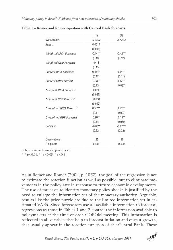
Results for the regressions are shown in Table 1. The sample comprises 125 COPOM meetings, from July 28, 1999 to November 30, 2011. The forecasts explain more than 40% of the change in the Selic rate. In com-parison to other studies, this value is higher than those found for the US and UK. Romer and Romer (2004) original study found a R2 of 0.28 for their equation, while Cloyne and Hürtgen (2014) report a figure of 0.29.

The second column on Table 1 shows the results considering all expla-natory variables, while on the third column I keep only the statistically significant ones. Overall the results show a strong reaction to forecasts of GDP growth and inflation for the current year. Changes in weighted forecasts for GDP and inflation were also significant, and also the level of the weighted forecast for inflation. The negative sign of the constant indicates a downward trend in the Selic rate over the period.



Table 1 – Romer and Romer equation with Central Bank forecasts

(1) (2)VARIABLES ∆ Selic ∆ SelicSelic t–1 0.0014

(0.016)

Weighted IPCA Forecast -0.44*** -0.42***(0.13) (0.12)

Weighted GDP Forecast -0.18(0.15)

Current IPCA Forecast 0.45*** 0.44***(0.12) (0.11)

Current GDP Forecast 0.33** 0.17***(0.13) (0.037)

∆Current IPCA Forecast 0.024(0.067)

∆Current GDP Forecast -0.058(0.042)

∆Weighted IPCA Forecast 0.56*** 0.55***(0.11) (0.097)

∆Weighted GDP Forecast 0.28** 0.13**(0.14) (0.059)

Constant -0.80** -0.87***(0.32) (0.23)

Observations 125 125R-squared 0.441 0.429

Robust standard errors in parentheses*** p<0.01, ** p<0.05, * p<0.1

As in Romer and Romer (2004, p. 1062), the goal of the regression is not to estimate the reaction function as well as possible, but to eliminate mo-vements in the policy rate in response to future economic developments. The use of forecasts to identify monetary policy shocks is justified by the need to enlarge the information set of the monetary authority. Arguably, results like the price puzzle are due to the limited information set in es-timated VARs. Since forecasters use all available information to forecast, regressions as those in Tables 1 and 2 control the information available to policymakers at the time of each COPOM meeting. This information is reflected in all variables that help to forecast inflation and output growth, that usually appear in the reaction function of the Central Bank. These



likely include the expected path of fiscal policy variables and also the ex-change rate over the forecast period. Even studies for Brazil that allowed for a larger information set, as the FAVAR estimated by Carvalho and Rossi Júnior (2009), did not include expectations, due to the small num-ber of observations at the time (Carvalho and Rossi Júnior 2009, pg. 291).

A second set of forecasts, also employed in the analysis, comes from the Focus survey, which on a daily basis disclosures forecasts for growth and inflation for several years ahead. The end of year forecasts were transfor-med on constant maturity forecasts. For each date in which the forecasts were available, I collect the forecasts for up to the longest year available.

𝑓𝑓𝑓𝑓𝑓𝑓𝑓𝑓𝑓𝑓𝑓𝑓𝑓𝑓𝑓𝑓𝑗𝑗+1(𝑚𝑚𝑓𝑓𝑚𝑚𝑓𝑓ℎ𝑖𝑖𝑦𝑦𝑓𝑓𝑓𝑓𝑓𝑓𝑗𝑗) = (12 − 𝑚𝑚𝑓𝑓𝑚𝑚𝑓𝑓ℎ(𝑑𝑑𝑓𝑓𝑓𝑓𝑓𝑓)12 ) ∗ 𝑓𝑓𝑓𝑓𝑓𝑓𝑓𝑓𝑓𝑓𝑓𝑓𝑓𝑓𝑓𝑓(𝑦𝑦𝑓𝑓𝑓𝑓𝑓𝑓𝑗𝑗) +

(𝑚𝑚𝑚𝑚𝑚𝑚𝑚𝑚ℎ(𝑑𝑑𝑑𝑑𝑚𝑚𝑑𝑑)12 ) ∗ 𝑓𝑓𝑓𝑓𝑓𝑓𝑓𝑓𝑓𝑓𝑓𝑓𝑓𝑓𝑓𝑓(𝑦𝑦𝑓𝑓𝑓𝑓𝑓𝑓𝑗𝑗+1)

(3)

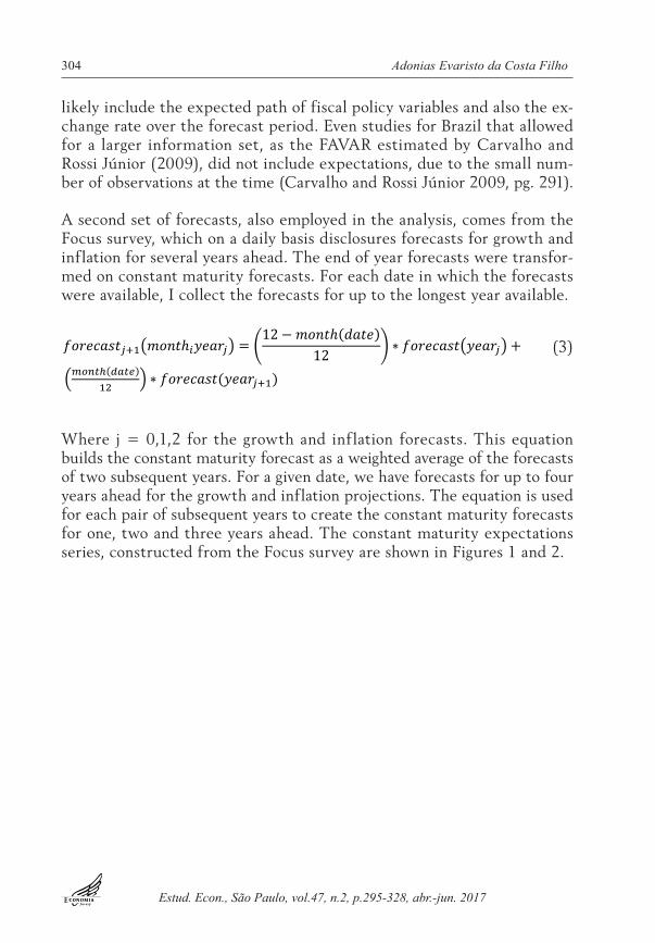
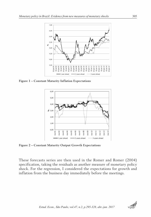
Where j = 0,1,2 for the growth and inflation forecasts. This equation builds the constant maturity forecast as a weighted average of the forecasts of two subsequent years. For a given date, we have forecasts for up to four years ahead for the growth and inflation projections. The equation is used for each pair of subsequent years to create the constant maturity forecasts for one, two and three years ahead. The constant maturity expectations series, constructed from the Focus survey are shown in Figures 1 and 2.



Figure 1 – Constant Maturity Inflation Expectations

0,00

1,00

2,00

3,00

4,00

5,00

6,00

nov-

01

nov-

02

nov-

03

nov-

04

nov-

05

nov-

06

nov-

07

nov-

08

nov-

09

nov-

10

nov-

11

nov-

12

nov-

13

nov-

14

%

1 year ahead 2-years ahead 3-years ahead

Figure 2 – Constant Maturity Output Growth Expectations

These forecasts series are then used in the Romer and Romer (2004) specification, taking the residuals as another measure of monetary policy shock. For the regression, I considered the expectations for growth and inflation from the business day immediately before the meetings.



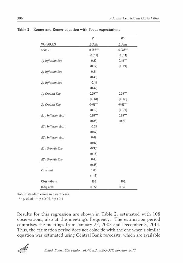
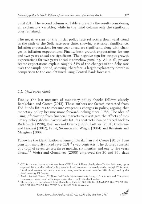
Table 2 – Romer and Romer equation with Focus expectations

(1) (2)

VARIABLES ∆ Selic ∆ Selic

Selic t–1 -0.056*** -0.038***

(0.017) (0.011)

1y Inflation Exp 0.22 0.19***

(0.17) (0.024)

2y Inflation Exp 0.21

(0.48)

2y Inflation Exp -0.48

(0.42)

1y Growth Exp 0.39*** 0.39***

(0.064) (0.063)

2y Growth Exp -0.62*** -0.52***

(0.12) (0.074)

∆1y Inflation Exp 0.98*** 0.89***

(0.35) (0.20)

∆2y Inflation Exp -0.55

(0.67)

∆3y Inflation Exp 0.49

(0.97)

∆1y Growth Exp -0.30*

(0.18)

∆2y Growth Exp 0.43

(0.35)

Constant 1.66

(1.15)

Observations 108 108

R-squared 0.553 0.543

Robust standard errors in parentheses*** p<0.01, ** p<0.05, * p<0.1

Results for this regression are shown in Table 2, estimated with 108 observations, also at the meeting’s frequency. The estimation period comprises the meetings from January 22, 2003 and December 3, 2014. Thus, the estimation period does not coincide with the one when a similar equation was estimated using Central Bank forecasts, which are available



until 2011. The second column on Table 2 presents the results considering all explanatory variables, while in the third column only the significant ones remained.

The negative sign for the initial policy rate reflects a downward trend in the path of the Selic rate over time, showing statistical significance. Inflation expectations for one year ahead are significant, along with chan-ges in inflation expectations. Finally, both growth expectations for one and two years ahead are significant. The negative sign for output growth expectations for two years ahead is somehow puzzling. All in all, private sector expectations explain roughly 54% of the changes in the Selic rate over the sample period, showing, therefore, a larger explanatory power in comparison to the one obtained using Central Bank forecasts.

2.2. Yield curve shock

Finally, the last measure of monetary policy shocks follows closely Barakchian and Crowe (2013). These authors use factors extracted from Fed Funds futures to measure exogenous changes in policy, arguing that monetary policy became more forward-looking since 1988. The idea of using information from financial markets to investigate the effects of mo-netary policy shocks, particularly futures contracts, can be traced back to Rudebusch (1998), Bagliano and Favero (1999), Kuttner (2001), Cochrane and Piazzesi (2002), Faust, Swanson and Wright (2004) and Brissimis and Magginas (2006).

Following the identification scheme of Barakchian and Crowe (2013), I use constant maturity fixed rate-CDI 6 swap contracts. The dataset consists of a total of seven tenors: three months, six months, and one to five years ahead.7,8 Vieira and Gonçalves (2008) employed the 30 and 360-days

6 CDI is the one day interbank rate from CETIP, and follows closely the effective Selic rate, up to a spread. Bets on the path of policy rates in Brazil are most commonly made through DI futures. I work with constant maturity rates swap rates, in order to overcome the difficulties posed by the fixed maturity DI futures.

7 Barakchian and Crowe (2013) use Fed Funds futures contracts for up to 5 months ahead. Therefore, I use more contracts and with longer maturities to build the shock series.

8 The series were downloaded from Bloomberg Tickers: BCSWEPD, BCSWGPD, BCSWFPD, BC-SWKPD, BCSWLPD, BCSWMPD and BCSWNPD Currency.



swap. Therefore, I substantially expand the analysis, in order to capture the full impact of monetary policy on the term structure.

As argued by the Barakchian and Crowe (2013), there are several reasons to take into account a range of maturities. It helps to minimize noise from a particular tenor, possibly stemming from term premium, liquidity dif-ferences, and also as a measure to capture both the impact of the change in the policy rate and the effects on long-term rates through expectations of the future path of short-term rates.

As in their analysis, a simple factor model was estimated via maximum likelihood, using the change in the swap rates in the neighborhood of each meeting as inputs, using the difference between the business day imme-diately after the meeting relative to the business day immediately before. Specifically, the model is:

s = φΛ ' + e (4)

Where s is the vector of the changes in swap rates for all maturities con-sidered (seven), φ is the vector of factors, Λ is the factor loading matrix and e is the vector of unique factors. The factor method is a way to bypass the need to model the entire yield curve, giving more importance to those maturities that exhibit a greater degree of comovement in extracting the factors. As in Barakchian and Crowe (2013), I identify the shock series as the first factor, which has the interpretation of the effect of monetary policy on the level of the term structure. The dataset used to construct this factor shock series is comprised of 108 observations (COPOM meet-ings) beginning in 2003 and ending in 2014. Even though for the shorter tenors the data goes back to 1999, for the longer maturities the series be-gin in the second half of 2002. This was a very volatile period in financial markets, due to uncertainty brought by the elections. Thus, I preferred to use 2003 as the starting point. The swap series which were used as inputs and the cumulated factors are shown in Figure 3.



Figure 3 – Swaps data

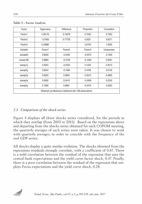
I found that two factors explain 92% of the total variance. Alone, the first factor (yield curve level) explains 75% of the total variance, while the second factor (yield curve slope) explains 17% of the total variance. As for the relevance of each variable in the factor, the analysis shows that short-term maturities account for the bulk of the first factor, while for the second factor the longest tenors play a more significant role. With the exception of the three and four year-ahead maturities, the other maturities display a significant common variability, above 90%, as one can infer from the unique variances in Table 1. Finally, the loadings indicate that the first factor exerts a positive influence on all maturities, whereas the second factor loads negatively the maturities up to two years ahead and positively from the three year swap onwards, therefore steepening the yield curve.



Table 3 – Factor Analysis

Factor Eigenvalue Difference Proportion Cumulative

Factor1 4.36176 3.14576 0.7250 0.7250

Factor2 1.21600 0.77720 0.2021 0.9271

Factor3 0.43880 . 0.0729 1.0000

Variable Factor1 Factor2 Factor3 Uniqueness

sswap90 0.8029 -0.4345 -0.2570 0.1005

sswap180 0.8883 -0.4109 -0.1259 0.0261

sswap1y 0.9354 -0.2425 0.1225 0.0513

sswap2y 0.8244 -0.1584 0.4709 0.0735

sswap3y 0.6253 0.0853 0.3410 0.4855

sswap4y 0.6932 0.5419 -0.0409 0.2242

sswap5y 0.7085 0.6881 -0.0472 0.0223

Obtained via Maximum Likelihood with 108 observations

2.3. Comparison of the shock series

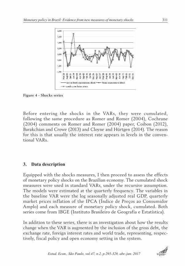
Figure 4 displays all three shocks series considered, for the periods in which they overlap (from 2003 to 2011). Based on the regressions above and departing from the shocks series obtained for each COPOM meeting, the quarterly averages of each series were taken. It was chosen to work with quarterly averages, in order to coincide with the frequency of the real GDP series.

All shocks display a quite similar evolution. The shocks obtained from the regressions residuals strongly correlate, with a coefficient of 0.87. There is a mild correlation between the residual of the regression that uses the central bank expectations and the yield curve factor shock, 0.47. Finally, there is a poor correlation between the residual of the regression that em-ploys Focus expectations and the yield curve shock, 0.28.



Figure 4 - Shocks series

Before entering the shocks in the VARs, they were cumulated, following the same procedure as Romer and Romer (2004), Cochrane (2004) comments on Romer and Romer (2004) paper, Coibon (2012), Barakchian and Crowe (2013) and Cloyne and Hürtgen (2014). The reason for this is that usually the interest rate appears in levels in the conven-tional VARs.

3. Data description

Equipped with the shocks measures, I then proceed to assess the effects of monetary policy shocks on the Brazilian economy. The cumulated shock measures were used in standard VARs, under the recursive assumption. The models were estimated at the quarterly frequency. The variables in the baseline VAR were the log seasonally adjusted real GDP, quarterly market prices inflation of the IPCA (Índice de Preços ao Consumidor Amplo) and each measure of monetary policy shock, cumulated. Both series come from IBGE (Instituto Brasileiro de Geografia e Estatística).

In addition to these series, there is an investigation about how the results change when the VAR is augmented by the inclusion of the gross debt, the exchange rate, foreign interest rates and world trade, representing, respec-tively, fiscal policy and open economy setting in the system.



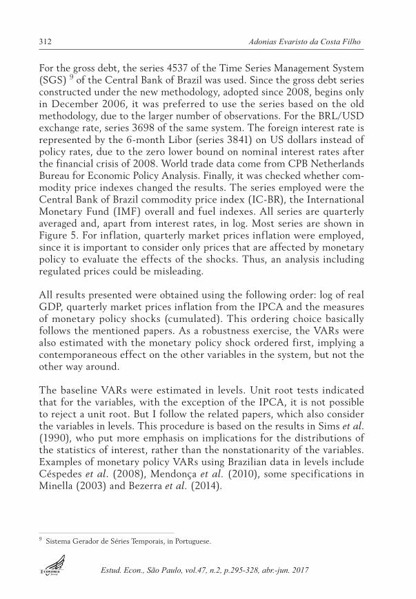
For the gross debt, the series 4537 of the Time Series Management System (SGS) 9 of the Central Bank of Brazil was used. Since the gross debt series constructed under the new methodology, adopted since 2008, begins only in December 2006, it was preferred to use the series based on the old methodology, due to the larger number of observations. For the BRL/USD exchange rate, series 3698 of the same system. The foreign interest rate is represented by the 6-month Libor (series 3841) on US dollars instead of policy rates, due to the zero lower bound on nominal interest rates after the financial crisis of 2008. World trade data come from CPB Netherlands Bureau for Economic Policy Analysis. Finally, it was checked whether com-modity price indexes changed the results. The series employed were the Central Bank of Brazil commodity price index (IC-BR), the International Monetary Fund (IMF) overall and fuel indexes. All series are quarterly averaged and, apart from interest rates, in log. Most series are shown in Figure 5. For inflation, quarterly market prices inflation were employed, since it is important to consider only prices that are affected by monetary policy to evaluate the effects of the shocks. Thus, an analysis including regulated prices could be misleading.

All results presented were obtained using the following order: log of real GDP, quarterly market prices inflation from the IPCA and the measures of monetary policy shocks (cumulated). This ordering choice basically follows the mentioned papers. As a robustness exercise, the VARs were also estimated with the monetary policy shock ordered first, implying a contemporaneous effect on the other variables in the system, but not the other way around.

The baseline VARs were estimated in levels. Unit root tests indicated that for the variables, with the exception of the IPCA, it is not possible to reject a unit root. But I follow the related papers, which also consider the variables in levels. This procedure is based on the results in Sims et al. (1990), who put more emphasis on implications for the distributions of the statistics of interest, rather than the nonstationarity of the variables. Examples of monetary policy VARs using Brazilian data in levels include Céspedes et al. (2008), Mendonça et al. (2010), some specifications in Minella (2003) and Bezerra et al. (2014).

9 Sistema Gerador de Séries Temporais, in Portuguese.



Figure 5 - Data

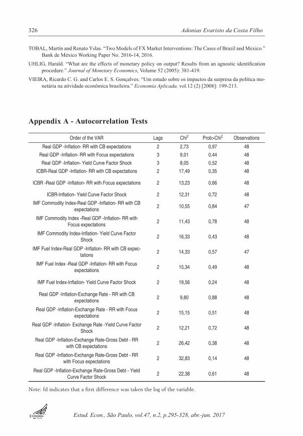
In almost all estimated VARs, stability conditions were satisfied. When that was not the case, some variables entered the model in first differen-ces, so as to satisfy stability. Lags were selected based on the AIC and BIC statistics. Appendix A displays the lags for each model, the p-value at the Lagrange Multipliers statistics, indicating the lack of autocorrelation, and any transformation to make the model stable.

4. Results

Figures 6 and 7 show the impulse response functions of the estimated VARs, with the monetary policy shocks ordered first and last, respectively. The baseline response is showed along with 95% confidence bands in gray.



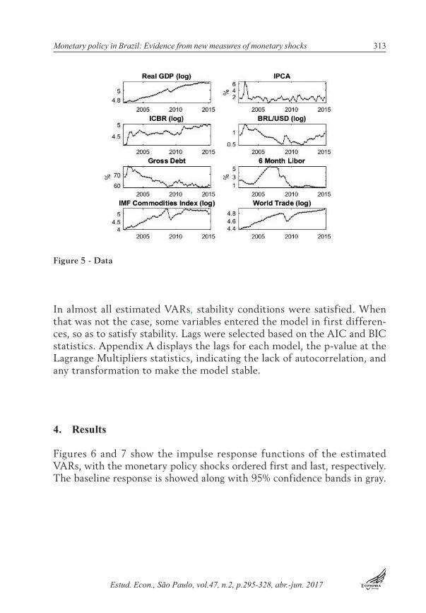
Figure 6 - Impulse Response Functions

Note: The first row shows the responses of the log of real GDP to a standardized monetary shock, while the second row displays the responses of inflation to the same shock. From left to right: RR shock with Central Bank expectations, RR shock with Focus expectations and yield curve factor shock.

In response to the measures of monetary policy shocks, real GDP declines, with a maximum impact of 0.5% until the fifth month after the shock. For inflation, the estimation shows a price puzzle for all shocks, with inflation initially increasing after the shock and then falling. The price puzzle is more pronounced for the response considering the RR shock with Central Bank expectations and very mild for the RR shock with market expec-tations and for the yield curve shock. One possibility for this behavior might lie in the estimation period of each model. While the VAR with RR central bank expectations was estimated from the 1999 Q3 to 2011 Q4, the VAR with RR market expectations was estimated from 2003 Q3 to 2014 Q4. The reason for the different sample is that the Central Bank of Brazil releases the technical presentations of COPOM meetings with a delay of four years, being 2011 the last year with complete data. On the other hand, the period for the model with RR market expectations was chosen to coincide with the availability of data for the yield curve, so that the models with RR with market expectations and with the yield curve shock were estimated using the same period.



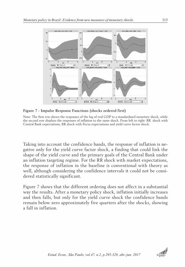
Figure 7 - Impulse Response Functions (shocks ordered first)


Taking into account the confidence bands, the response of inflation is ne-gative only for the yield curve factor shock, a finding that could link the shape of the yield curve and the primary goals of the Central Bank under an inflation targeting regime. For the RR shock with market expectations, the response of inflation in the baseline is conventional with theory as well, although considering the confidence intervals it could not be consi-dered statistically significant.

Figure 7 shows that the different ordering does not affect in a substantial way the results. After a monetary policy shock, inflation initially increases and then falls, but only for the yield curve shock the confidence bands remain below zero approximately five quarters after the shocks, showing a fall in inflation.



5. Including commodity prices

In the next step, commodity price indexes were included in the esti-mated VARs in order to check robustness of the results. Traditionally, a commodity price index is used to “solve” the price puzzle, in the sense that the puzzle is explained by an anticipation of an increase in inflation, to which the central bank responded by raising rates, creating a positi-ve correlation between the increase in interest rates and the increase in inflation. Commodity prices were then used as a variable that helps to forecast inflation, and including them in the system corrected the price puzzle. Hanson (2004) examines the link between indicators that help to predict inflation and their ability to solve the price puzzle, showing a poor correlation between them, implying that the puzzle might not be due to a lack of a variable that predicts inflation in the VAR. In our case, by construction, the RR shocks already excludes the expected component of inflation and output growth since they are based on the residuals of a regression of interest rates changes on official and private forecasts. Thus, one could argue that there is no major reason for including a commodity price index in the estimated VARs. Regardless of this potential argument, it was done as a robustness exercise.

In these models, the commodity price index was ordered first in the sys-tem, in log level. The commodity price indexes employed were the IC-BR (Índice de Commodities Brasil) from the Central Bank of Brazil, the IMF overall and fuel commodity price index. Thus the VARs were estimated with the following order: each one of the commodity price indexes, log of real GDP, inflation and one of the three measures of monetary po-licy shocks, implicitly implying that the commodity price index is the most exogenous variable in the system, under the Choleski identification scheme.

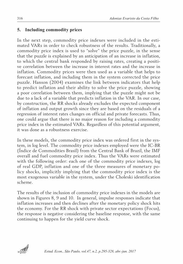
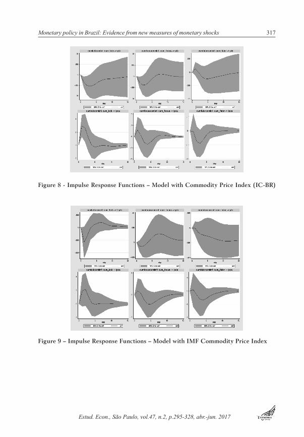
The results of the inclusion of commodity price indexes in the models are shown in Figures 8, 9 and 10. In general, impulse responses indicate that inflation increases and then declines after the monetary policy shock hits the economy. For the RR shock with private sector expectations (Focus), the response is negative considering the baseline response, with the same continuing to happen for the yield curve shock.



Figure 8 - Impulse Response Functions – Model with Commodity Price Index (IC-BR)

Figure 9 – Impulse Response Functions – Model with IMF Commodity Price Index



Figure 10 – Impulse Response Functions – Model with IMF Fuel Price Index


6. Augmenting the VARs with exchange rate, fiscal and external variables

In order to provide additional robustness for the results, VARs including additional variables were estimated. The first one employed the baseline specification of Luporini (2008), with the following order: output, infla-tion rate, nominal exchange rate as measured by the Real/ US Dollar and the shock series, replacing the interest rate in her paper. This order is also consistent with the one employed in the comparison of VAR and FAVAR models in Carvalho and Rossi Júnior (2009, p. 297). It was also included a measure of global trade and US interest rates exogenously in the VAR, also following Luporini (2008), intending to see how the results change in an open economy VAR.



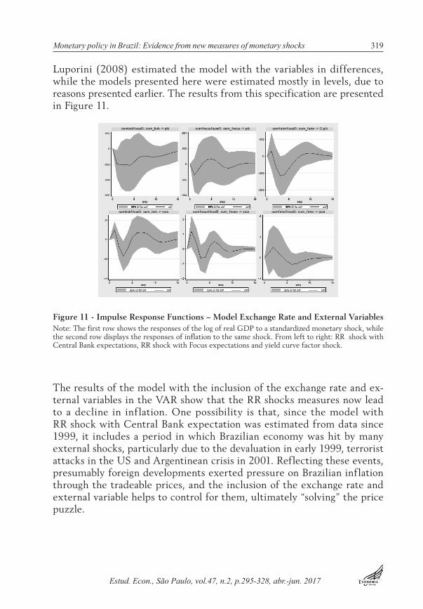
Luporini (2008) estimated the model with the variables in differences, while the models presented here were estimated mostly in levels, due to reasons presented earlier. The results from this specification are presented in Figure 11.

Figure 11 - Impulse Response Functions – Model Exchange Rate and External VariablesNote: The first row shows the responses of the log of real GDP to a standardized monetary shock, while the second row displays the responses of inflation to the same shock. From left to right: RR shock with Central Bank expectations, RR shock with Focus expectations and yield curve factor shock.

The results of the model with the inclusion of the exchange rate and ex-ternal variables in the VAR show that the RR shocks measures now lead to a decline in inflation. One possibility is that, since the model with RR shock with Central Bank expectation was estimated from data since 1999, it includes a period in which Brazilian economy was hit by many external shocks, particularly due to the devaluation in early 1999, terrorist attacks in the US and Argentinean crisis in 2001. Reflecting these events, presumably foreign developments exerted pressure on Brazilian inflation through the tradeable prices, and the inclusion of the exchange rate and external variable helps to control for them, ultimately “solving” the price puzzle.



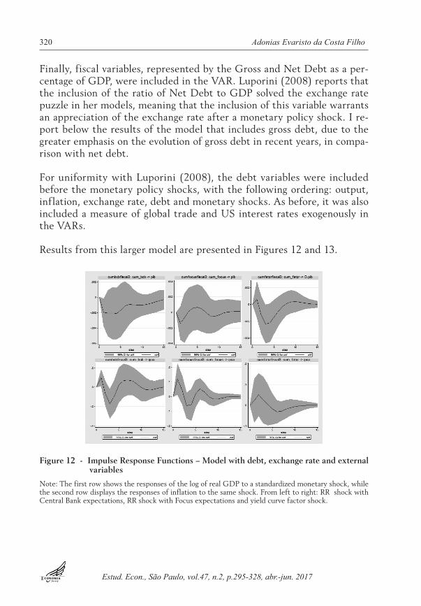
Finally, fiscal variables, represented by the Gross and Net Debt as a per-centage of GDP, were included in the VAR. Luporini (2008) reports that the inclusion of the ratio of Net Debt to GDP solved the exchange rate puzzle in her models, meaning that the inclusion of this variable warrants an appreciation of the exchange rate after a monetary policy shock. I re-port below the results of the model that includes gross debt, due to the greater emphasis on the evolution of gross debt in recent years, in compa-rison with net debt.

For uniformity with Luporini (2008), the debt variables were included before the monetary policy shocks, with the following ordering: output, inflation, exchange rate, debt and monetary shocks. As before, it was also included a measure of global trade and US interest rates exogenously in the VARs.

Results from this larger model are presented in Figures 12 and 13.

Figure 12 - Impulse Response Functions – Model with debt, exchange rate and external variables




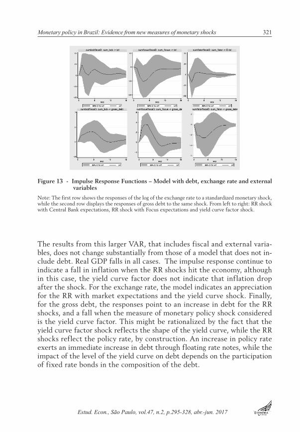
Figure 13 - Impulse Response Functions – Model with debt, exchange rate and external variables

Note: The first row shows the responses of the log of the exchange rate to a standardized monetary shock, while the second row displays the responses of gross debt to the same shock. From left to right: RR shock with Central Bank expectations, RR shock with Focus expectations and yield curve factor shock.

The results from this larger VAR, that includes fiscal and external varia-bles, does not change substantially from those of a model that does not in-clude debt. Real GDP falls in all cases. The impulse response continue to indicate a fall in inflation when the RR shocks hit the economy, although in this case, the yield curve factor does not indicate that inflation drop after the shock. For the exchange rate, the model indicates an appreciation for the RR with market expectations and the yield curve shock. Finally, for the gross debt, the responses point to an increase in debt for the RR shocks, and a fall when the measure of monetary policy shock considered is the yield curve factor. This might be rationalized by the fact that the yield curve factor shock reflects the shape of the yield curve, while the RR shocks reflect the policy rate, by construction. An increase in policy rate exerts an immediate increase in debt through floating rate notes, while the impact of the level of the yield curve on debt depends on the participation of fixed rate bonds in the composition of the debt.



7. Conclusion

The purpose of this paper was to investigate the effects of monetary policy shocks on the Brazilian economy, taking a comprehensive approach, by using a variety of monetary policy shocks. The main contribution to the literature was to build new measures of monetary policy shocks.

Based on expectations for output growth and inflation, both private and official, measures based on Romer and Romer’s (2004) approach were built for Brazil. Measures of monetary policy shocks based on this methodology received renewed attention recently in the studies of Coibon (2012) for the US and Cloyne and Hürtgen (2014) for the UK. For the RR shocks, it was built a new database of forecasts of inflation and GDP growth from the Central Bank of Brazil staff data. These forecasts appear in the technical presentations for monetary policy meetings (COPOM) and began to be released after the Access of Information Law. They are presented in the Appendix for other researchers. For private forecasts, constant maturity series of expectations of inflation and output growth were built, shown in Figures 1 and 2.

In addition to the shocks based on Romer and Romer’s (2004) methodo-logy, a yield curve measure of monetary policy shocks was built, following closely the approach undertaken by Barakchian and Crowe (2013) for the US, intending to see how the yield curve reaction to monetary policy decisions feeds back into the economy. This follows the tradition of using financial market data to identify the effects of monetary policy. This part of the paper thus investigates how the yield curve reaction to monetary policy reverberates on the Brazilian economy.

Regarding the results, it was found that after a standardized monetary policy shock, real GDP declines for almost 0.5% after the shock hits the economy. For inflation, the results show a price puzzle for all RR shocks measures in a small VAR, with inflation initially increasing and then falling after the shock. Only for the yield curve shock the response is negative, considering that the 95% confidence bands remain below zero after the shock. This result could suggest that a monetary policy strategy that ma-ximizes its impact on the yield curve might produce better outcomes in terms of reducing inflation, a potential avenue for research in the future. The inclusion of commodity prices in the models did not change substan-tially the results, with inflation falling under the baseline response for



the RR with market expectations and the yield curve shocks. VARs that included the exchange rate, external variables, and gross debt showed that inflation declined for the RR shocks, with the response being statistically significant. The exchange rate appreciates for the RR shocks under the baseline, consistent with theory. Debt increases after the RR shocks, and it was argued that the different response for the yield curve shocks might be related to the nature of this shock, which is based on the yield curve.

The price puzzle found in some specifications of this paper could be ratio-nalized, at least to some extent, by the existence of a cost channel of mo-netary policy (Barth and Ramey, 2001) operating in Brazil, with inflation initially increasing and then falling after a monetary policy shock. This explanation argues that there is nothing wrong with the price puzzle per se, or that the source of the puzzle in not the misspecification of the mo-dels, but only reflects that firms must finance their wage bill in advance of production. Thus, after an increase in the interest rate, some production costs also increase, ultimately leading to an increase in inflation, until the demand effects dominate and inflation begins to fall. Considering the findings of this paper, a possible extension of this work could be the esti-mation of a DSGE model that includes a cost channel of monetary policy, along the lines of Rabanal (2007) and Henzel et al. (2009).910

Another possible explanation for the price puzzle that emerged recently lies in the foreign exchange (FX) intervention in Brazil. Tobal and Yslas (2016) argue that the Brazilian model of FX intervention entails inflatio-nary costs, creating noise in the relationship between interest rates and inflation.

10 Rabanal (2007) estimates a DSGE model for the US and the Euro area and finds little evidence of a cost channel of monetary policy. In his Bayesian estimation of the model, only implausible values of the parameter associated with the cost channel would lead to a price puzzle. On the other hand, Henzel et al. (2009) estimate a DSGE model with a banking sector and a cost channel for the euro area by minimizing the distance of the impulse responses of a VAR and those from the model, and show that a parameter configuration without the cost channel is not successful in replicating the price puzzle observed in the VAR model.



References

BAgLIAno, Fabio C. and Carlo A. Favero. “Information from Financial Markets and VAR Measures of Mo-netary Policy.” European Economic Review, 43(4-6), [1999]:825-37.

BARAkChIAn, S. Mahdi and Christopher Crowe. “Monetary policy matters: Evidence from new shocks data.” Journal of Monetary Economics, 60 (2013): 950–966.

BARth, Marvin J., and Valerie A. Ramey. “the Cost Channel of Monetary transmission.” nBER Macroeco-nomics Annual, 2001.

BERnAnkE, Ben.S., and Alan .S. Blinder. “the Federal Funds Rate and the Channels of Monetary transmis-sion.” American Economic Review 82 (1992): 901-921.

BERnAnkE, Ben S. and Ilian Mihov. “Measuring Monetary Policy.” The Quarterly Journal of Economics, Vol.113, no 3 (Aug. 1998): 869-902.

BERnAnkE, Ben S., Jean Boivin, and Piotr Eliasz. “Measuring the Effects of Monetary Policy: A Factor-Aug-mented Vector Autoregressive (FAVAR) Approach.” The Quarterly Journal of Economics, Volume 120 (1) [2005]: 387-422.

BEzERRA, Jocildo Fernandes; Igor Ézio Maciel Silva and Ricardo Chaves Lima. “os efeitos da política mo-netária sobre o produto no Brasil: evidência empírica usando restrição de sinais.” Rev. econ. Contemp. V. 18, n. 2 (Aug. 2014): 296-316, Rio de Janeiro.

BRISSIMIS, Sophocles n., and nicholas S. Magginas. “Forward-Looking Information in VAR Models and the Price Puzzle.” Journal of Monetary Economics, Volume 53(6) [2006]:1225- 1234.

CARVALho, Marina and J. Rossi Júnior. “Identification of Monetary Policy Shocks and Their Effects: FAVAR Methodology for the Brazilian Economy.” Brazilian Review of Econometrics 29(2009): 285-313.

CÉSPEdES, Brisne; Elcyon Lima; Alexis Maka. “Monetary policy, inflation and the level of economic activity in Brazil after the Real Plan: stylized facts from SVAR models.” Rev. Bras. Econ. V. 62, n. 2, June 2008, Rio de Janeiro.

ChRIStIAno, Lawrence J.; Martin Eichenbaum and Charles Evans. “the Effects of Monetary Policy Shocks: Evidence from the Flow of Funds.” Review of Economics and Statistics, Volume 78(1) [1996]: 16-34.

ChRIStIAno, Lawrence, Martin Eichenbaum, and Charles Evans. “Monetary Policy Shocks: What have We Learned, and to What End?” In John B taylor and Michael Woodford (eds.), 65-148. Handbook of Monetary Economics: Elsevier Science, 1999.

CLoynE, James and Patrick hürtgen. “the macroeconomics effects of monetary policy: a new measure for the United kingdom.” Bank of England Working Paper no. 493, 2014.

CoIBIon, olivier. “Are the Effects of Monetary Policy Shocks Big or Small?” American Economic Journal: Macroeconomics, American Economic Association, vol. 4(2) [2012]: 1-32, April.

CoChRAnE, John h. “What do the VARs mean? Measuring the output effect of monetary policy.” Journal of Monetary Economics 41(1998): 277-300.

CoChRAnE, John and Monika Piazzesi. “The FED and Interest Rates – A High Frequency Identification.” American Economic Review, 92(2) [2002]: 90-95.

CoChRAnE, John. “Comments on ‘A new measure of monetary shocks: derivation and implications’ By Christina Romer and david Romer.” Paper presented at nBER EFg meeting, on July 17, 2004.Available at:http://faculty.chicagobooth.edu/john.cochrane/research/papers/talk_notes_new_measure_2.pdf. Accessed on September 7, 2016.

CoChRAnE, John. “Do Higher Interest Rates Raise or Lower Inflation?” (2016). Available at: http://faculty.chicagobooth.edu/john.cochrane/research/papers/fisher.pdf Accessed on September 7, 2016.

CySnE, Rubens P. “Is there a Price Puzzle in Brazil? An Application of Bias-Corrected Bootstrap.” Ensaio Econômico da EPgE n.577, 2004.



CySnE, Rubens P. “What happens After the Central Bank of Brazil Increases the target Interbank Rate by 1%?” Ensaio Econômico da EPgE n.577, 2005.

dIAS, daniel A. and João B. duarte. “the Effect of Monetary Policy on housing tenure Choice as an Explanation for the Price Puzzle.” International Finance Discussion Papers 1171, 2016.

EIChEnBAUM, Martin. “Comment on interpreting the macroeconomic time series facts: the effects of monetary policy.” European Economic Review, v. 36(5) [1992]:1001-1011.

FAUSt, Jon, Eric t. Swanson and Jonathan h. Wright. “Identifying VARs based on high frequency futures data.” Journal of Monetary Economics, Volume 51(6) [2004]: 1107-113, September 2004.

FERnAndES, Marcelo and Juan toro. “o mecanismo de transmissão monetária na economia brasileira pós-Plano Real.” Rev. Bras. Econ., Rio de Janeiro, v. 59(1) [2005], Mar. 2005.

gIoRdAnI, Paolo. “An Alternative Explanation of the Price Puzzle.” Journal of Monetary Economics, Volume 51 (2004): 1271-1296.

hAnSon, Michael S. “the ‘Price Puzzle’ Reconsidered.” Journal of Monetary Economics, Volume 51(2004): 1385-1413.

hEnzEL, Steffen; oliver hlsewig; Eric Mayer and timo Wollmershuser. “the price puzzle revisited: Can the Cost Channel Explain a Rise in Inflation after a Monetary Policy Shock?” Journal of Macroeconomics, Volume 31(2) [2009]: 268-289.

kUttnER, kenneth n. “Monetary policy surprises and interest rates: Evidence from the Fed funds futures markets.” Journal of Monetary Economics, Volume 47(3) [2001]: 523-544, June 2001.

LEEPER, Eric M. “Narrative and VAR Approaches to Monetary Policy: Common Identification Problems.” Journal of Monetary Economics 40(1997): 641:657.

LUPoRInI, Viviane. “the Monetary transmission Mechanism in Brazil: evidence from a VAR analysis.”Estudos Econômicos (USP. Impresso), v. 38 (2008): 07-30.

MEndonçA, Mario; Luís Medrano and Adolfo Sachsida. “Efeitos da Política Monetária na Economia Brasi-leira: Resultados de um Procedimento de Identificação Agnóstica.” Pesquisa e Planejamento Econômico, 40(3) [2010]:367-394.

MInELLA, André. “Monetary policy and inflation in Brazil (1975-2000): a VAR estimation.” Rev. Bras. Econ., Rio de Janeiro, v. 57(3): 605-635, Sept. 2003.

RABAnAL, Pau. “Does inflation increase after a monetary policy tightening? Answers based on an estimated dSgE model.” Journal of Economics Dynamics Control, Volume 31(2007): 906-937.

RAMEy, Valerie. “Macroeconomic Shocks and their Propagation.” nBER Working Paper 21978, 2016.RoMER, Christina d., and david h. Romer. “does Monetary Policy Matter? A new test in the Spirit of Friedman

and Schwartz.” nBER Macroeconomics Annual, 1989.RoMER, Christina d., and david h. Romer. “A new Measure of Monetary Shocks: derivation and Implications.”

American Economic Review, Volume 94(4) [2004]: 1055-1084.RUdEBUSCh, glenn d. “do measures of monetary policy in a VAR make sense?” International Economic

Review 39 (1998): 907-931.SIMS, Christopher A.; John h. Stock; Mark W. Watson. “Inference in linear time series models with some unit

roots.” Econometrica 58 (1) [1990]: 113–144.SIMS, Christopher A. “Interpreting the macroeconomic time series facts: the effects of monetary policy.” Euro-

pean Economic Review, Volume 36 (5) [1992]: 975-1000.tAyLoR, John. “discretion versus policy rules in practice.” Carnegie-Rochester Conference Series on Public

Policy, n.39 (1993): 195-214. thAPAR, Aditi. “Using private forecasts to estimate the effects of monetary policy.” Journal of Monetary

Economics 55 (2008): 806–824.



toBAL, Martín and Renato yslas. “two Models of FX Market Interventions: the Cases of Brazil and Mexico.” Bank de México Working Paper no. 2016-14, 2016.

UhLIg, Harald. “What are the effects of monetary policy on output? Results from an agnostic identification procedure.” Journal of Monetary Economics, Volume 52 (2005): 381-419.

VIEIRA, Ricardo C. g. and Carlos E. S. gonçalves. “Um estudo sobre os impactos da surpresa da política mo-netária na atividade econômica brasileira.” Economia Aplicada, vol.12 (2) [2008]: 199-213.

Appendix A - Autocorrelation Tests

Order of the VAR Lags Chi2 Prob>Chi2 Observations

Real GDP -Inflation- RR with CB expectations 2 2,73 0,97 48

Real GDP -Inflation- RR with Focus expectations 3 9,01 0,44 48

Real GDP -Inflation- Yield Curve Factor Shock 3 8,05 0,52 48

ICBR-Real GDP -Inflation- RR with CB expectations 2 17,49 0,35 48

ICBR -Real GDP -Inflation- RR with Focus expectations 2 13,23 0,66 48

ICBR-Inflation- Yield Curve Factor Shock 2 12,31 0,72 48

IMF Commodity Index-Real GDP -Inflation- RR with CB expectations

2 10,55 0,84 47

IMF Commodity Index -Real GDP -Inflation- RR with Focus expectations

2 11,43 0,78 48

IMF Commodity Index-Inflation- Yield Curve Factor Shock

2 16,33 0,43 48

IMF Fuel Index-Real GDP -Inflation- RR with CB expec-tations

2 14,33 0,57 47

IMF Fuel Index -Real GDP -Inflation- RR with Focus expectations

2 15,34 0,49 48

IMF Fuel Index-Inflation- Yield Curve Factor Shock 2 19,56 0,24 48

Real GDP -Inflation-Exchange Rate - RR with CB expectations

2 9,80 0,88 48

Real GDP -Inflation-Exchange Rate - RR with Focus expectations

2 15,15 0,51 48

Real GDP -Inflation- Exchange Rate -Yield Curve Factor Shock

2 12,21 0,72 48

Real GDP -Inflation-Exchange Rate-Gross Debt - RR with CB expectations

2 26,42 0,38 48

Real GDP -Inflation-Exchange Rate-Gross Debt - RR with Focus expectations

2 32,83 0,14 48

Real GDP -Inflation-Exchange Rate-Gross Debt - Yield Curve Factor Shock

2 22,38 0,61 48

Note: fd indicates that a first difference was taken the log of the variable.



Appendix B - Database from the technical presentations of COPOM meetings

copom ipca_t ipca_t+1 ipca_pond pib_t pib_t+1 pib_pond23/06/1999 7,60 7,60 0,7 0,7028/07/1999 7,90 7,90 0,7 0,7001/09/1999 7,80 7,80 0,5 0,5006/10/1999 7,80 4,50 5,05 0,5 0,5010/11/1999 7,98 5,85 6,03 0,5 0,5015/12/1999 8,94 6,20 6,20 0,8 0,8019/01/2000 6,20 6,20 3,3 3,3016/02/2000 6,20 6,20 3,3 3,3022/03/2000 6,20 6,20 3,3 3,3019/04/2000 6,20 6,20 3,6 3,6024/05/2000 6,00 6,00 3,6 3,6020/06/2000 5,80 5,80 3,6 3,6019/07/2000 5,60 5,60 3,6 3,6023/08/2000 6,54 6,54 3,8 3,8020/09/2000 6,79 6,79 3,8 3,8018/10/2000 6,19 6,19 3,8 3,8022/11/2000 6,28 6,28 3,8 3,9 3,8920/12/2000 6,06 3,81 3,81 3,8 3,9 3,9017/01/2001 4,00 4,00 3,9 3,9014/02/2001 4,09 4,09 3,9 3,9021/03/2001 4,20 4,20 3,9 3,9018/04/2001 4,50 4,50 4,3 4,3023/05/2001 5,63 5,63 2,2 2,2020/06/2001 5,80 5,80 2,8 2,8018/07/2001 5,87 5,87 2,5 2,5022/08/2001 6,32 6,32 2,1 2,1019/09/2001 6,59 6,59 1,9 1,9017/10/2001 6,46 6,46 2 2 2,0021/11/2001 7,35 7,35 2 2,2 2,1818/12/2001 7,35 4,60 4,60 2 2,5 2,5023/01/2002 4,49 4,49 2,5 2,5020/02/2002 4,77 4,77 2,5 2,5020/03/2002 5,09 5,09 2,5 2,5017/04/2002 5,56 5,56 2,7 2,7022/05/2002 5,46 5,46 2,4 2,4019/06/2002 5,47 5,47 2,2 2,2017/07/2002 5,81 5,81 1,8 1,8021/08/2002 6,43 6,43 1,5 1,5018/09/2002 6,64 4,49 5,03 1,5 1,5023/10/2002 7,62 5,58 5,92 1,3 2,1 1,9720/11/2002 9,78 6,54 6,81 1,5 2,7 2,6018/12/2002 12,48 8,46 8,46 1,6 2,8 2,8022/01/2003 9,70 9,70 2,8 2,8019/02/2003 11,28 11,28 2,6 2,6019/03/2003 11,47 11,47 2,2 2,2023/04/2003 12,00 12,00 2,2 2,2021/05/2003 11,96 11,96 2 2,0018/06/2003 11,48 11,48 1,5 1,5023/07/2003 9,77 9,77 1,5 1,5020/08/2003 9,06 9,06 1 1,0017/09/2003 9,38 9,38 0,6 0,6022/10/2003 9,52 9,52 0,6 0,6019/11/2003 9,13 6,43 6,66 0,8 3,5 3,2817/12/2003 9,17 6,11 6,11 0,3 3,5 3,5021/01/2004 6,11 6,11 3,5 3,5018/02/2004 6,49 6,49 3,5 3,5017/03/2004 6,29 6,29 3,5 3,5014/04/2004 6,53 6,53 3,5 3,5019/05/2004 6,44 6,44 3,5 3,5016/06/2004 6,61 6,61 3,5 3,5021/07/2004 6,96 6,96 3,75 3,75

copom ipca_t ipca_t+1 ipca_pond pib_t pib_t+1 pib_pond



18/08/2004 6,96 6,96 3,75 3,7515/09/2004 7,37 7,37 4,4 4,4020/10/2004 7,24 7,24 4,4 4,4017/11/2004 7,28 7,28 4,7 4,7015/12/2004 7,40 5,81 5,81 5 4 4,0019/01/2005 5,72 5,72 4 4,0016/02/2005 5,88 5,88 4 4,0016/03/2005 5,88 5,88 4 4,0020/04/2005 6,00 6,00 4 4,0018/05/2005 6,34 6,34 4 4,0015/06/2005 6,26 6,26 3,4 3,4020/07/2005 5,73 5,73 3,4 3,4017/08/2005 5,50 5,50 3,4 3,4014/09/2005 5,46 5,46 3,4 3,4019/10/2005 5,44 5,44 3,4 3,4023/11/2005 5,61 5,61 3,4 3,4014/12/2005 5,71 5,71 2,6 2,6018/01/2006 4,50 4,50 4 4,0008/03/2006 4,50 4,50 4 4,0019/04/2006 4,50 4,50 4 4,0031/05/2006 4,50 4,50 4 4,0019/07/2006 4,00 4,00 4 4,0030/08/2006 3,79 3,79 4 4,0018/10/2006 2,97 2,97 3,5 3,5029/11/2006 3,20 4,13 4,05 3,5 4,2 4,1424/01/2007 4,13 4,13 3,8 3,8007/03/2007 4,00 4,00 4,1 4,1018/04/2007 4,10 4,10 4,5 4,5006/06/2007 3,63 3,63 4,7 4,7018/07/2007 3,72 3,72 4,7 4,7005/09/2007 4,06 4,06 4,7 4,7017/10/2007 3,87 3,87 4,7 4,7005/12/2007 3,99 4,02 4,02 4,7 4,5 4,5023/01/2008 4,42 4,42 4,5 4,5005/03/2008 4,33 4,33 4,5 4,5016/04/2008 4,67 4,67 4,8 4,8004/06/2008 5,81 5,81 4,8 4,8023/07/2008 6,54 6,54 4,8 4,8010/09/2008 6,13 6,13 4,8 4,1 4,2829/10/2008 6,12 6,12 5 4,1 4,2510/12/2008 6,19 5,17 5,17 5,6 3,2 3,2021/01/2009 4,62 4,62 3,2 3,2011/03/2009 4,59 4,59 2 2,0029/04/2009 4,42 4,42 0,8 0,8010/06/2009 4,37 4,37 0,8 0,8022/07/2009 4,53 4,53 0,8 0,8002/09/2009 4,26 4,26 0,8 0,8021/10/2009 4,22 4,22 0,8 0,8009/12/2009 4,31 4,31 -0,3 5,8 5,8027/01/2010 4,71 4,71 5,8 5,8017/03/2010 5,23 5,23 5,8 5,8028/04/2010 5,51 5,51 6,6 6,6009/06/2010 5,87 5,87 6,6 6,6021/07/2010 5,11 5,11 7,3 7,3001/09/2010 4,83 4,83 7,3 7,3020/10/2010 5,17 4,59 4,69 7,3 7,3008/12/2010 5,87 4,59 4,59 7,3 4,5 4,5019/01/2011 4,93 4,93 4,5 4,5002/03/2011 5,46 5,46 4 4,0020/04/2011 6,24 6,24 4 4,0008/06/2011 6,24 6,24 4 4,0020/07/2011 6,24 6,24 4 4,0031/08/2011 6,33 6,33 4 4,0019/10/2011 6,44 6,44 4 4,0030/11/2011 6,49 5,27 5,37 3 3,00

estudos econômicos (são paulo) this is an open access

Documents