ethanol 2g: development of a methodology to evaluate the ... · ethanol 2g: development of a...

Ethanol 2G: Development of a methodology to evaluate

the morphology of lignocellulosic substrates

Ana Sofia Brazão Borrego

Thesis to obtain the Master of Science Degree in

Chemical Engineering

Supervisors: Dr. Damien Hudebine

Dr. Nadège Charon

Prof. João Carlos Moura Bordado

Examination Committee

Chairperson:

Supervisor:

Member of the Committee:

Prof. Sebastião Manuel Tavares Silva Alves

Prof. João Carlos Moura Bordado

Dr. Maria Margarida Pires dos Santos Mateus

September 2015

This page was intentionally left blank.

You have to learn the rules of the game.

And then you have to play better than anyone else.

Albert Einstein (1879-1955)

I

ACKNOWLEDGMENTS

I appreciate this awesome chance that IFP Energies nouvelles provided me. Damien and Nadège,

the achievement of this work will not be possible without your significant collaboration. I’m grateful for

the continuous learning that you gave me, the challenges, the confidence and all suggestions. You

made this internship an enriching experience. Also a special thanks to Marie-Olive that supported me

in my first days and always cared about my good being. I extend my gratitude to the excellent people

from Elbaite (Serge, Amandine, Karine). A particular thanks to Michel for his availability and good

humor. Generally, the support from both R12 and R05 was indispensable.

I want to thank deeply to the person that made possible that this opportunity took part of my life.

Prof. Filipa Ribeiro: thank for your teaching during last years and dedication to allow this extraordinary

experience to me and to my colleagues. Also an word to Joana Fernandes and Vitor Costa that

welcomed us in IFP in the best way. To my supervisor from Instituto Superior Técnico, Prof. João

Bordado, I thanks for the given suggestions and the final revision of this work.

This period of time made me grow up professionally but also personally. I’m grateful to the

portuguese community that integrated us (Ruben, Sonia, Leonor, Max, Leonel, Mafalda,…). I also had

the opportunity to meet people that encouraged me to learn French language and costumes (Fabien,

Mathieu, Swetan,…). The coffees and lunches together were also important, a word to Larissa, Alexis

and Raido. To my office partners, Rami, Romain, and Laure, that taught me the first words in french.

To all my friends from the university (particularly, Mariana, Filipe and Bernardo) and my friends from

ever (Ana Marta, Ana Luísa, Sara, …). People, you are incredible! Thanks for sharing extraordinary

moments with me.

A huge thank to my family in Lyon: Loios, Solange, Casinhas, David, Catarina, Joana, Diogo. For

the sharing of experiences during these six months, the adventures in the trips, the everyday dinners

together, every moments, always together. Thank you all for the friendship.

I reserve this last paragraph to express my biggest acknowledgments. To whom that told me (and

still remember me every time) to work and put all my best qualities in everything that I do. The people

who deserve all my respect: Mãe, Pai, Mano. Pedro, I thank you for believing me and for your

unconditional support.

II


III

RESUMO

Este trabalho teve como objectivo o desenvolvimento de um método que permite caracterizar a

área superficial disponível de substratos linhocelulósicos e relacioná-la com a reactividade desses

substratos na hidrólise enzimática.

Numa primeira fase, foi efectuado um estudo bibliográfico extensivo que permitiu identificar os

métodos disponíveis para o propósito. Uma técnica baseada na exclusão molecular de solutos foi

proposta com o objectivo de determinar o volume acessível nos materiais linhocelulósicos a

moléculas sonda de diferentes tamanhos. Foram exploradas duas abordagens distintas baseadas na

utilização de um substrato saturado ou seco. A segunda abordagem não existe na literatura e foi

adaptada com sucesso a partir da primeira.

A metodologia utilizando um substrato seco foi testada com uma celulose comercial (Alphacel

C40) e palha de trigo (nativa e pré-tratada a 160 oC, lavada e não lavada). Também foi proposta uma

equação modelo que descreve a distribuição de poros por tamanhos. Foi feito um estudo completo

com a Alphacel, no entanto, é necessário mais estudo sobre os restantes substratos. A técnica

caracteriza-se pelo longo tempo de espera (1 dia por molécula sonda, 10 dias por substrato). Para

solucionar este problema, foram sugeridas diversas optimizações neste trabalho.

A metodologia proposta é reprodutível e foi validada para a Alphacel. Este trabalho deverá ser

completado com a aplicação do método na caracterização de outros substratos pré-tratados, com o

objectivo de obter uma base de comparação da eficiência dos pré-tratamentos.

PALAVRAS-CHAVE:

Biocombustíveis; Etanol 2G; Linhocelulose; Área acessível; Exclusão de solutos.

IV


V

ABSTRACT

This work focused on the development of a methodology that allows to characterize the available

surface area of lignocellulosic substrates and to relate it with their reactivity on enzymatic hydrolysis.

Firstly, an extended literature review was done on the methods used for this purpose. A method

based on solute exclusion was proposed and aimed to measure the accessible volume of

lignocellulosic materials by using chemical probes of different sizes. Two approaches were explored

based on a saturated or a dried substrate. The second method does not exist in literature and was

adapted with success from the first one.

The methodology using a dried substrate was tested using a commercial cellulose (Alphacel C40)

and wheat straw (native and pretreated at 160 oC, non-washed and washed). A model equation was

also proposed in order to describe pore size distribution. A complete study was done on Alphacel but

more studies are still required for the other substrates. The main drawback of this technique is its long

experimental standby time (1 day per probe, 10 days per substrate). To solve this issue, several

optimizations were suggested in this work.

The methodology proposed is reproducible and was validated for Alphacel. The present work shall

be completed with the characterization of other pretreated substrates, in order to provide a basis to

compare pretreatment’s effectiveness.

KEYWORDS:

Biofuels; Ethanol 2G; Lignocellulose; Available area; Solute-exclusion.

VI


VII

Table of contents

Acknowledgments .................................................................................................................................... I

Resumo .................................................................................................................................................. III

Abstract .................................................................................................................................................... V

Table of contents ................................................................................................................................... VII

List of Symbols and Abbreviations ......................................................................................................... IX

List of Figures ......................................................................................................................................... XI

List of Tables ........................................................................................................................................ XIII

1 Introduction ....................................................................................................................................... 1

2 Literature Review ............................................................................................................................. 3

Energy Context .................................................................................................................... 3

Lignocellulosic Biomass ...................................................................................................... 4

Production Processes of Ethanol 2G ................................................................................... 6

Pretreatment, the first key decision ............................................................................. 7

Enzymatic hydrolysis, the bottleneck of the process ................................................. 10

Process configurations .............................................................................................. 12

Measurement of Porosity and Surface Area ..................................................................... 14

BET method using nitrogen adsorption ..................................................................... 14

Mercury porosimetry .................................................................................................. 15

Simons’ stain ............................................................................................................. 16

Solute exclusion technique ........................................................................................ 17

Size-exclusion chromatography – SEC ..................................................................... 18

Other techniques ....................................................................................................... 18

Solute Exclusion Technique .............................................................................................. 19

State of the art ........................................................................................................... 19

Comparison of protocols ............................................................................................ 21

Conclusion and aim of the study ....................................................................................... 22

3 Pretreatment of the substrate ......................................................................................................... 23

Thermochemical pretreatment ........................................................................................... 23

Acid hydrolysis ................................................................................................................... 25

Enzymatic hydrolysis ......................................................................................................... 26

VIII

4 Method to determine the pore volume ........................................................................................... 29

Materials and methods ...................................................................................................... 29

Methodology for substrate in saturated form ..................................................................... 30

Water retention value method – WRV ....................................................................... 30

Methodology for substrate in dried form ............................................................................ 33

Probe solutions analysis .................................................................................................... 34

5 Results of Substrate Porosity ......................................................................................................... 39

Determination of pore volume ........................................................................................... 39

Saturated substrate method ...................................................................................... 39

Dried substrate method ............................................................................................. 40

Pore volume distribution .................................................................................................... 43

Determination of specific surface area .............................................................................. 54

Summary and discussion .................................................................................................. 55

6 Conclusions and Future Prospects ................................................................................................ 63

7 References ..................................................................................................................................... 65

8 Appendix ........................................................................................................................................ 71

Results from enzymatic hydrolysis .................................................................................... 71

Probe molecules ................................................................................................................ 71

Results from water retention value method ....................................................................... 72

Calibration curves (refractometry) ..................................................................................... 74

Saturated substrate methodology – Alphacel .................................................................... 75

Dried substrate methodology – Alphacel ........................................................................... 76

Dried substrate methodology – Non-washed native wheat straw ..................................... 78

Dried substrate methodology – Washed native wheat straw ............................................ 83

Dried substrate methodology – Wheat straw pretreated at 160 °C and washed .............. 85

Pore volume distributions for dried substrate methodology .............................................. 86

IX

List of Symbols and Abbreviations

Symbol Description Units

1G First-generation [ ]

2G Second-generation [ ]

AFM Atomic force microscopy [ ]

AV Average value *

BET Brunauer-Emmett-Teller [ ]

CBM Cellulose-binding module [ ]

Ceq Equilibrium concentration g/100mL or %w/v

Cf Concentration of the final solution g/100mL or %w/v

Cg Concentration in glucose of the final solution g/L

Ci Concentration of the initial solution g/100mL or %w/v

CLSM Confocal laser scanning microscopy [ ]

D Diameter of probe molecule Å

DSC Differential scanning calorimeter [ ]

s Substrate porosity [ ]

FSP Fiber saturation point mL or mL/g mds

H Humidity %

ID Sample identification [ ]

k Constant of pore volume distribution curves 1/Å

mds Mass of dried substrate g

mf Final mass of substrate g

mi Initial mass of substrate g

ms Mass of substrate g

mss Mass of saturated substrate g

mtotal Total mass of the mixture g

nD Refractive index at 20°C [ ]

nD’ Refractive index at 20°C with correction [ ]

NMR Nuclear magnetic resonance [ ]

nprobe Amount of probe in solution mol

PEG Polyethylene glycol [ ]

s Bulk density of the substrate g/mL

SD Standard deviation *

SE Solute exclusion [ ]

SEC Size-exclusion chromatography [ ]

SEM Scanning electron microscopy [ ]

SSA Specific surface area m2/g

*depends on the measured parameter

X

Symbol Description Units

SHF Separate hydrolysis and fermentation [ ]

SSF Simultaneous saccharification and fermentation [ ]

t Time h

T Temperature °C

TEM Transmission electron microscopy [ ]

TGC Fluorescent protein [ ]

Va Accessible pore volume mL or mL/g mds

Ve Exterior volume mL or mL/g mds

Vi Inaccessible pore volume mL or mL/g mds

Vi,max Maximum inaccessible pore volume mL or mL/g mds

Vp Pore volume mL

Vsol Volume of solution mL

Vsol,i Volume of initial probe solution mL

WRV Water retention value g/g or %

XI

List of Figures

Figure 2-1: Projected world energy-related CO2 emissions (Mton/year) [5]............................................ 3

Figure 2-2: Evolution in consumption of biofuels in transportation sector, in EU28 [7]. .......................... 4

Figure 2-3: Arrangement of the mainly constituents of lignocellulosic biomass in the cell wall [12]. ...... 5

Figure 2-4: Scheme from vegetal cells to glucose monomer – adapted from [17, 18]............................ 6

Figure 2-5: Biocatalysed-production of fuel ethanol from lignocellulosic biomass [20]. .......................... 7

Figure 2-6: Categories of pretreatment methods for lignocellulosic biomass – according to [10, 21, 22].

................................................................................................................................................................. 8

Figure 2-7: Simplified scheme of the impact of pretreatment on biomass [22]. .................................... 10

Figure 2-8: SSF in relation to other process options [26]. ..................................................................... 12

Figure 2-9: Scheme of ethanol 2G production process in SHF configuration – adapted from [17]. ..... 12

Figure 2-10: Schematic representation of an SSF process [26]. .......................................................... 13

Figure 2-11: Gas adsorption models [31]. ............................................................................................. 14

Figure 2-12: Mercury intrusion porosimetry [34].................................................................................... 15

Figure 2-13: Example of light microscope image of Simons' stained mechanical pulp fibers [38]........ 16

Figure 2-14: Representation of the accessibility to the pores of a substrate using solute exclusion [43].

............................................................................................................................................................... 17

Figure 2-15: Layout for the size-exclusion system proposed by Yang and his co-workers [46]. .......... 18

Figure 2-16: Schematic illustration of pore distribution curve to solute excluded from the pores [53]. . 20

Figure 2-17: General scheme of the different steps to perform solute exclusion. ................................. 21

Figure 3-1: Pilot unit U868 for thermochemical pretreatment of lignocellulosic substrates. ................. 23

Figure 3-2: Samples obtained by different severities of acid pretreatment. .......................................... 24

Figure 3-3: Yield in dry substrate after pretreatment. ............................................................................ 25

Figure 3-4: Schematic representation of two step acid hydrolysis. ....................................................... 25

Figure 3-5: Glucostat used to measure the concentration in glucose of the samples. ......................... 27

Figure 3-6: Glucose yield on enzymatic hydrolysis (Appendix 8.1). ...................................................... 27

Figure 4-1: Scheme of the methodology for substrate in saturated form. ............................................. 30

Figure 4-2: Evolution of mass substrate during drying, for Avicel PH101 (Table 8-4, Appendix 8.3). .. 32

Figure 4-3: Evolution of mass substrate during drying, for Alphacel C40 (Table 8-6, Appendix 8.3). .. 32

Figure 4-4: Results from determination of WRV for Avicel PH101 (Table 8-7, Appendix 8.3). ............. 33

Figure 4-5: Results from determination of WRV for Alphacel C40 (Table 8-8, Appendix 8.3). ............. 33

Figure 4-6: Scheme of the methodology for substrate in dried form. .................................................... 34

Figure 4-7: Refractometer used to measure the refractive index of solutions. ..................................... 34

Figure 4-8: Sample recovered after decantation and prepared to analyze in refractometer. ............... 35

Figure 4-9: Linear correlation between refractive index and concentration for PEG 35000 (02/07/2015).

............................................................................................................................................................... 35

Figure 4-10: Linear correlation between refractive index and concentration for PEG 35000

(10/07/2015). ......................................................................................................................................... 36

Figure 4-11: Evolution of calibration curves for PEG 200 (between 28/05/2015 and 15/07/2015). ...... 36

Figure 4-12: Examples of calibration curves for the different probes. ................................................... 38

XII

Figure 5-1: Distribution of values for water retention method, for Alphacel (Table 8-10, Appendix 8.5).

............................................................................................................................................................... 39

Figure 5-2: Calibration curve and results for experiment SE02 (Table 8-10, Appendix 8.5). ............... 40

Figure 5-3: Scheme of a porous substrate and penetration of molecules. ........................................... 41

Figure 5-4: Expected increasing in accessible porous volume by type of substrate. ............................ 42

Figure 5-5: Example of a series of samples in a trial. ........................................................................... 43

Figure 5-6: Pore volume distribution for pulp fibers exposed to different conditions [40]. .................... 44

Figure 5-7: Scheme representative of different levels of porosity. ........................................................ 45

Figure 5-8: Pore volume distribution for Alphacel (Table 8-21, Appendix 8.10). .................................. 46

Figure 5-9: Pore volume distribution for Alphacel (Table 8-21, Appendix 8.10). .................................. 47

Figure 5-10: Pore volume distribution of celluloses (Table 5-2) [19]. .................................................... 47

Figure 5-11: Pore volume distribution for non-washed native wheat straw (Table 8-22, Appendix 8.10).

............................................................................................................................................................... 48


............................................................................................................................................................... 48

Figure 5-13: Pore volume distribution for non-washed native wheat straw, with refractive index

correction – all points included (Table 8-23, Appendix 8.10). ............................................................... 49

Figure 5-14: Pore volume distribution for non-washed native wheat straw, with refractive index

correction. (Table 8-23, Appendix 8.10) ................................................................................................ 50

Figure 5-15 : Pore volume distribution for washed native wheat straw (Table 8-24, Appendix 8.10). .. 51

Figure 5-16: Pore volume distribution for washed native wheat straw, with refractive index correction

(Table 8-25, Appendix 8.10). ................................................................................................................. 51

Figure 5-17: Pore volume distribution for washed and pretreated wheat straw (Table 8-26, Appendix

8.10). ...................................................................................................................................................... 52

Figure 5-18: Pore volume distribution for Alphacel and different wheat straw products. ...................... 53

Figure 5-19: Pore volume distribution for pulp fibers – zoom of Figure 5-6 [40]. .................................. 53

Figure 5-20: Schematic representation of the structural features of the cellulose particle surface [19].

............................................................................................................................................................... 54

Figure 5-21: Accessible pore volume of corn stover, measured by solute exclusion [42]. ................... 55

Figure 5-22: Influence of substrate quantity in final concentration of probe. ........................................ 57

Figure 5-23: Influence of the ratio mass of substrate by volume of solution in final concentration of

probe. ..................................................................................................................................................... 58

Figure 5-24: Experimental issue on stirring. .......................................................................................... 59

Figure 5-25: Comparison between a native and a pretreated wheat straw samples, after stirring. ...... 59

Figure 5-26: Comparison between a washed (1’) and a non-washed (1) native wheat straw

supernatants. ......................................................................................................................................... 60

Figure 5-27: Pore volume distribution for Alphacel (Table 8-21, Appendix 8.10). ................................ 61

Figure 8-1: Correlation obtained for PEG probes by power curve. ....................................................... 72

XIII

List of Tables

Table 2-1: Composition of the different components in lignocellulosic biomasses – adapted from [15]. 5

Table 2-2: Preparation conditions for substrates and probe solutions. ................................................. 21

Table 3-1: Operating conditions of the pretreatment. ............................................................................ 24

Table 3-2: Results from acid hydrolysis. ............................................................................................... 26

Table 4-1: Molecular weights and solution diameters of probes used (Appendix 8.2).......................... 29

Table 4-2: Initial conditions of substrates to water retention value method. ......................................... 31

Table 4-3: Linear correlations between refractive index and concentration for PEG 200 (Figure 4-11).

............................................................................................................................................................... 36

Table 5-1: Exterior and maximal pore volume determined for the substrates. ..................................... 42

Table 5-2: Fiber saturation point by solute exclusion technique, from literature. .................................. 43

Table 5-3: Fiber saturation point from different pretreatments. ............................................................. 44

Table 5-4: Types of porosity in solids [61]. ............................................................................................ 45

Table 5-5: Example of exterior and total porous volume determination, for Alphacel (Table 8-11). ..... 46

Table 5-6: Contribution of soluble components for refractive index measurements. ............................ 51

Table 5-7: Results of specific surface area from N2 gas adsorption, in this work. ................................ 54

Table 5-8: Specific surface area from literature, for wheat straw, by N2 gas adsorption. ..................... 55

Table 5-9: Example of concentrations of probe (Appendix 8.6; Appendix 8.7). .................................... 56

Table 5-10: Influence of substrate quantity in final concentration of probe. .......................................... 57

Table 5-11: Day work plan to performed one experiment with the dried substrate methodology. ........ 60

Table 5-12: Day work plan to performed two experiments by dried substrate methodology. ............... 61

Table 8-1: Glucose yield from enzymatic hydrolysis for the pretreated samples. ................................. 71

Table 8-2: Solution molecular diameters of probes from literature [40, 53]. ......................................... 71

Table 8-3: Drying of substrate WRV1, for Avicel PH101. ...................................................................... 72



Table 8-6: Drying of substrate WRV4, for Alphacel C40. ...................................................................... 73

Table 8-7: Results of WRV for Avicel PH101. ....................................................................................... 73

Table 8-8: Results of WRV for Alphacel C40. ....................................................................................... 73

Table 8-9: Linear correlations between refractive index and concentration of probe. .......................... 74

Table 8-10: Results from saturated substrate methodology, for Alphacel. ........................................... 75

Table 8-11: Results from dried substrate methodology, for Alphacel (part 1). ...................................... 76

Table 8-12: Results from dried substrate methodology, for Alphacel (part 2). ...................................... 77

Table 8-13: Results from dried substrate methodology, for non-washed native wheat straw (part 1). . 78



Table 8-16: Results from dried substrate methodology, for non-washed native wheat straw – nD

correction (part 1). ................................................................................................................................. 81

Table 8-17: Results from dried substrate methodology, for non-washed native wheat straw – nD

correction (part 2). ................................................................................................................................. 82

XIV

Table 8-18: Results from dried substrate methodology, for washed native wheat straw. ..................... 83

Table 8-19: Results from dried substrate methodology, for washed native wheat straw – nD correction.

............................................................................................................................................................... 84

Table 8-20: Results from dried substrate methodology, for wheat straw pretreated at 160 °C and

washed. ................................................................................................................................................. 85

Table 8-21: Pore volume distribution data for Alphacel. ....................................................................... 86

Table 8-22: Pore volume distribution data for non-washed native wheat straw. ................................... 86

Table 8-23: Pore volume distribution data for non-washed native wheat straw – nD correction. ......... 87

Table 8-24: Pore volume distribution data for washed native wheat straw. .......................................... 87

Table 8-25: Pore volume distribution data for washed native wheat straw – nD correction. ................ 87

Table 8-26: Pore volume distribution data for washed and pretreated wheat straw. ............................ 87

1

1 INTRODUCTION

Due to the energy context in the XXI century, fossil fuels have started to be replaced and

renewable alternatives are being seriously considered. In this field, the interest for second-generation

fuels obtained from lignocellulosic biomass has increased: one possible way to that is using this

biomass to produce ethanol from a biological way (pretreatment, enzymatic hydrolysis, fermentation,

distillation). However, the technology costs are still an obstacle, particularly in the pretreatment step.

In order to improve the digestibility of the lignocellulosic biomass, i.e. degradation of cellulose and

hemicelluloses, a pretreatment of the substrate has to be performed. This will increase the total yield

of monomeric sugars in the hydrolysis step. Afterwards, an understanding about the role of each

enzymatic family (cellobiohydrolases, endoglucanases, -glucosidases) is needed to improve

enzymatic hydrolysis.

Since porosity and surface area are reported as key-parameters in the mentioned process, the

main goal of this study was to ascertain methodologies suitable to characterize lignocellulosic

substrates. More particularly, elaborate a methodology that allows to determine the morphology of a

given substrate expeditiously. With this, a basis to compare pretreatment’s effectiveness can be

established, as well, to relate it with the reactivity of the substrate in hydrolysis.

⃝ ⃝ ⃝

Hence, a bibliographic study was done to explain general concepts about biofuels and its insertion

in the current energy context. Particularly, the second-generation is discussed. Then, a review about

the different methodologies available to characterize the substrates surface area was done (second

chapter).

Before to proceed for the essence of the work, a previous work was done in order to prepare the

substrates and is explained in chapter three. Subsequently, for the chosen technique (solute

exclusion), preliminary assays were performed to define the adequate conditions of experimentation.

The materials and methodologies used are described in chapter four. Using a statistical treatment, the

data obtained from the measurement of pore distribution is reported in chapter five and deliberated.

Lastly, the main conclusions obtained by this work are presented and discussed. To complete this

study, future prospects and suggestions were proposed.

2


3

2 LITERATURE REVIEW

Energy Context

In 2008 [1], no one had a definitive answer for the question “when will lignocellulosic ethanol

become economically viable?”. In 2013 [2], the world’s largest cellulosic ethanol production facility

opened at Crescentino, Italy, and currently, cellulosic ethanol is being produced on commercial scale

in Europe, USA and Brazil.

Current energy context

Today fossil fuels are the dominant energy sources, meeting more than 80% of the world’s energy

demand and is set to grow by 37% by 2040 (IEA, 2014). Nevertheless, fossil fuels are non-renewable

and their reserves are limited: at the current consumption rates, the supply of petroleum, natural gas,

and coal will only be able to last for another 45, 60, and 120 years, respectively (IEA, 2013).

Furthermore, the carbon dioxide represents 77% of greenhouse gas emissions and this

tremendous amount of emissions has been released essentially from fossil fuels combustion [3] –

Figure 2-1. This resulted in elevating the atmospheric CO2 concentration. Consequently, renewable

alternatives should be seriously considered. The recent energy independence and climate change

policies encourage development and utilization of renewables such as bioenergy, solar and wind

energy [4].

Figure 2-1: Projected world energy-related CO2 emissions (Mton/year) [5].

In this context, the EU supported the utilization of renewable energies proposing a replacement of

5.75%, by 2010, of the classical fuels by substitute products, as biofuels, (2003/30/CE), as well, fixing

a goal of 10% incorporation of renewable energies in the total of automobile fuels to 2020

(2009/28/CE). Recently, EU countries have agreed on a new renewable energy target of at least 37%

by 2030 [6]. By over the years, it is visible an increasing in the consumption of biofuels – Figure 2-2.

4

Figure 2-2: Evolution in consumption of biofuels in transportation sector, in EU28 [7].

Nowadays, there is utmost of alternative energy resources which are cheap, renewable and limit

pollution. Biomass is inserted in the context of renewables and is being considered as an important

resource all over the world. Actually, biomass it is the fourth largest source of energy after coal,

petroleum and natural gas, providing about 14% of the world’s primary energy consumption [8].

Second generation (2G) biofuels

It is known that renewables will continue to play a key role in reducing the greenhouse gas

emissions and their sources are abundant in the world. By this, the history of ethanol as a biofuel

dates back to the early days of the automobile era [8]. It is expected that biofuels can provide up to

27% of world transportation fuel, in 2050 (IEA, 2011).

Currently, the first-generation (1G) biofuels are already in the market in industrial scale, and the

second-generation (2G) is emerging, being extensively researched in the past two decades [9, 10].

Still, to minimize the adverse impacts, they must be produced in a sustainable way.

In contrast to ethanol 1G made from food crops, cellulosic ethanol is manufactured from non-food

plant materials (such as agricultural residues or energy crops). This lignocellulosic feedstock is

abundant, however it consists in a complex and very resistant structure (cellulose, hemicelluloses and

lignin) that needs to be broken down into simple sugars before fermentation and distillation.

Lignocellulosic Biomass

Cellulose, hemicelluloses and lignin are the three mainly constituents of lignocellulosic biomass

(along with small amounts of proteins, pectin, extractives and ash). These polymers, which are

associated each other, compose a complex and very resistant structure – Figure 2-3.

Cellulose is a glucose polymer and the mainly constituent of lignocellulosic biomass. It consists of

parts with a crystalline structure and parts with an amorphous structure [9, 11]. This polymer is a linear

chain of D-glucose subunits linked by -1,4 glycosidic bonds [11, 12].

Hemicelluloses are composed by different sugars like pentoses (C5 sugars such as xylose and

arabinose), hexoses (C6 sugars such as glucose, mannose and galactose) and acid sugars. These

5

components serve as a connection between the lignin and the

cellulose fibers and give the whole cellulose-hemicellulose-

lignin network more rigid [11].

Lignin is, after cellulose and hemicelluloses, one of the

most abundant polymers in nature and this main purpose is to

give the plant structural support [11]. It fills the spaces in the

cell wall between cellulose and hemicelluloses [12]. In this

way, lignin provides further strength to plant cell walls, but

hinders the enzymatic hydrolysis of carbohydrates [13].

As said above, plant cell walls are composed mostly of

lignocellulose which is the most abundant organic material on

Earth [8, 12, 14], being available from different sources –

Table 2-1. The composition of lignocellulosic biomass directly

depends on its origin:

Table 2-1: Composition of the different components in lignocellulosic biomasses – adapted from [15].

Lignocellulosic

biomass

Cellulose

(%w/w)

Hemicelluloses

(%w/w)

Lignin

(%w/w)

Wheat straw 33 23 17

Corn cob 45 35 15

Newspapers 40-55 25-40 18-30

Miscanthus 45 30 21

The nature of lignocellulosic material makes the pretreatment (section 2.3.1) a crucial step [16] due

to the physical and chemical barriers caused by the close association of the main components.

Figure 2-3: Arrangement of the mainly constituents of lignocellulosic biomass in the cell wall [12].

6

Cellulose, a complex substrate

The complex material named cellulose presents various levels of organization – Figure 2-4. Three

levels can be distinguished [17]: macroscopic scale, that are the cellulose particles, nanometric scale,

corresponding to the microfibers scale, and molecular scale that corresponds to the cellulose chain.

Figure 2-4: Scheme from vegetal cells to glucose monomer – adapted from [17, 18].

There are different morphologic cellulose parameters which develop an important role in the

reactivity of the substrate during hydrolysis. By this, the variety in physico-chemical characteristics

reveals the requirement of pretreatment technologies to help in the rapid and efficient conversion of

carbohydrate polymers into fermentable sugars [13, 19].

The main parameters include the crystallinity, the surface area, the degree of swelling, the degree

of polymerization and the size of the particles. These parameters are exploited later (section 2.3.2),

with a discussion of their influence in enzymatic hydrolysis step.

Production Processes of Ethanol 2G

Inversely to the production processes of first-generation ethanol, the sugars are not directly

accessible to fermentation in second-generation. The production of ethanol from lignocellulosic

material consists of mainly five different steps, namely, pretreatment, (enzymatic) hydrolysis,

fermentation, product separation, and post-treatment of the liquid fraction – Figure 2-5.

7

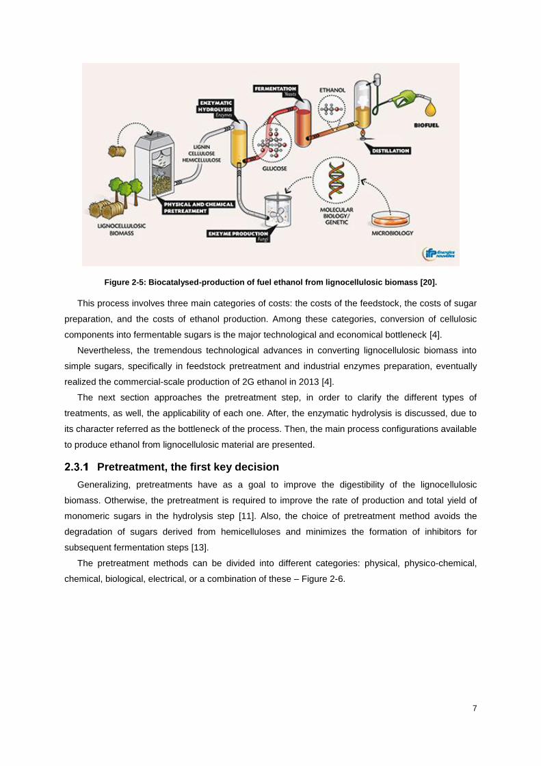
Figure 2-5: Biocatalysed-production of fuel ethanol from lignocellulosic biomass [20].

This process involves three main categories of costs: the costs of the feedstock, the costs of sugar

preparation, and the costs of ethanol production. Among these categories, conversion of cellulosic

components into fermentable sugars is the major technological and economical bottleneck [4].

Nevertheless, the tremendous technological advances in converting lignocellulosic biomass into

simple sugars, specifically in feedstock pretreatment and industrial enzymes preparation, eventually

realized the commercial-scale production of 2G ethanol in 2013 [4].

The next section approaches the pretreatment step, in order to clarify the different types of

treatments, as well, the applicability of each one. After, the enzymatic hydrolysis is discussed, due to

its character referred as the bottleneck of the process. Then, the main process configurations available

to produce ethanol from lignocellulosic material are presented.

Pretreatment, the first key decision

Generalizing, pretreatments have as a goal to improve the digestibility of the lignocellulosic

biomass. Otherwise, the pretreatment is required to improve the rate of production and total yield of

monomeric sugars in the hydrolysis step [11]. Also, the choice of pretreatment method avoids the

degradation of sugars derived from hemicelluloses and minimizes the formation of inhibitors for

subsequent fermentation steps [13].

The pretreatment methods can be divided into different categories: physical, physico-chemical,

chemical, biological, electrical, or a combination of these – Figure 2-6.

8

Figure 2-6: Categories of pretreatment methods for lignocellulosic biomass – according to [10, 21, 22].

PRETREATMENT

PHYSICAL

milling

chipping

grinding

extrusion

microwave oven

electron beam irradiation

PHYSICO-CHEMICAL

steam explosion

wet oxidation

liquid hot water (LHV)

ammonia fiber explosion (AFEX)

ammonia recycle percolation

aqueous ammonia

organosolv

CO2 explosion

CHEMICAL

alkali

dilute acid

concentrated acid

organic solvents

ozonolysis

oxidative delignification

wet oxidation

BIOLOGICAL

fungal

bio-organosolv

ELECTRICAL HYBRIDS

9

Physical pretreatment allows to increase the accessible surface area, as well the pore size of

lignocellulosic materials. Also, the crystallinity and degree of polymerization of cellulose is reduced

using this pretreatment method, increasing the reactivity of the substrate in enzymatic hydrolysis. This

method of fragmentation can greatly increase the accessible surface area [19], depending on the

porosity and cellulose particle size. However, this mechanical method is unattractive due to its high-

energy requirement and capital costs [10, 21].

Chemical pretreatment employs different chemical agents (such as acids, alkalis, ozone, among

others). This method has become one of the most promising to improve the biodegradability of

cellulose, by removing lignin and/or hemicelluloses, and decreasing the degree of polymerization and

crystallinity of cellulose. However, there are limitations associated to this method: it requires lower-cost

chemical reagents [13], and they must be recovered to make the pretreatment economically feasible

[10]. Following this, inorganic acids, such as H2SO4 or HCl, have been preferably used [21] and dilute

acid pretreatment (along with steam explosion) is one of the most widely studied method.

Physico-chemical pretreatment consists in a combination of the last methods and allows to dissolve

hemicelluloses and makes modifications in lignin structure, which provides an improved accessibility of

the cellulose for hydrolytic enzymes. The type of combination selected depends on the process

conditions and the solvents used that affect the physical and chemical properties of the biomass [10].

These methods are considerably more effective than physical and the steam explosion is the most

studied method of this type [21].

Biological pretreatment is mostly associated with the action of fungi that are capable of producing

enzymes to degrade lignin, hemicelluloses and polyphenols present in the biomass [10]. In

comparison with the pretreatments described above, the main advantages are that requires low

energy and the yield in desired products is high. However, the process is very slow and requires

careful control of growth conditions and large space to perform [21], limiting its application at industrial

level.

These methods have been investigated and reviewed by several researchers and authors [10, 11,

13, 23] and, among all, chemical pretreatment has been proven to be a promising one.

Due to the context of this study, the next section focus on the dilute acid pretreatment, since it was

the method used to prepare the substrates in this work.

10

Chemical pretreatment – dilute acid

Acid pretreatment particularly enhances the hydrolysis [13] and dilute acid pretreatment is one of

the oldest, simplest and frequently employed technique in biofuel production due to its efficiency [8,

23]. Additionally, H2SO4 and HCl have been preferably used for biomass pretreatment [21].

The treatment consists in adding a quantity of acid to the biomass (between 0.2 %w/w to 2.5

%w/w, depending if it is diluted or concentrated) and continuous stirring at temperatures between 130

°C and 210 °C [11].

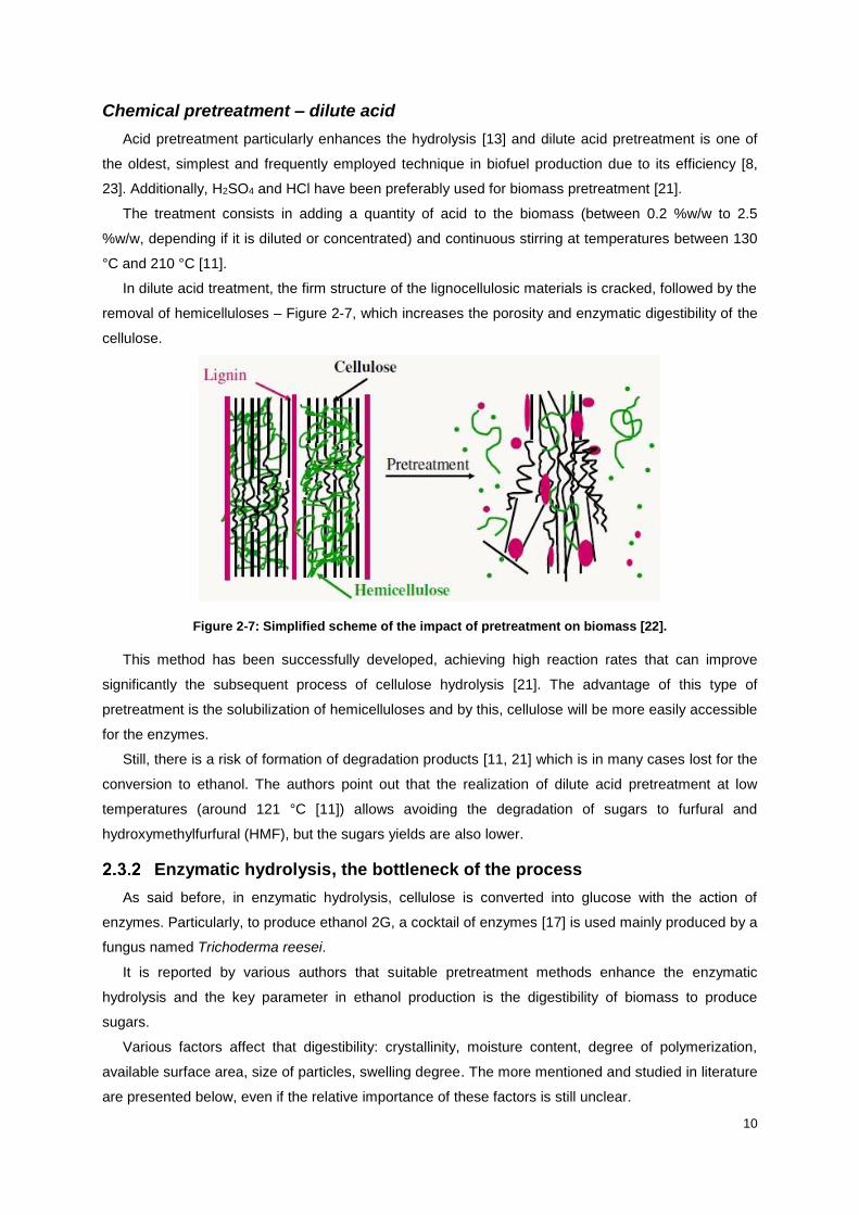
In dilute acid treatment, the firm structure of the lignocellulosic materials is cracked, followed by the

removal of hemicelluloses – Figure 2-7, which increases the porosity and enzymatic digestibility of the

cellulose.

Figure 2-7: Simplified scheme of the impact of pretreatment on biomass [22].

This method has been successfully developed, achieving high reaction rates that can improve

significantly the subsequent process of cellulose hydrolysis [21]. The advantage of this type of

pretreatment is the solubilization of hemicelluloses and by this, cellulose will be more easily accessible

for the enzymes.

Still, there is a risk of formation of degradation products [11, 21] which is in many cases lost for the

conversion to ethanol. The authors point out that the realization of dilute acid pretreatment at low

temperatures (around 121 °C [11]) allows avoiding the degradation of sugars to furfural and

hydroxymethylfurfural (HMF), but the sugars yields are also lower.

Enzymatic hydrolysis, the bottleneck of the process

As said before, in enzymatic hydrolysis, cellulose is converted into glucose with the action of

enzymes. Particularly, to produce ethanol 2G, a cocktail of enzymes [17] is used mainly produced by a

fungus named Trichoderma reesei.

It is reported by various authors that suitable pretreatment methods enhance the enzymatic

hydrolysis and the key parameter in ethanol production is the digestibility of biomass to produce

sugars.

Various factors affect that digestibility: crystallinity, moisture content, degree of polymerization,

available surface area, size of particles, swelling degree. The more mentioned and studied in literature

are presented below, even if the relative importance of these factors is still unclear.

11

Lignin and hemicelluloses content

As can be seen is Figure 2-3, most of the lignin is concentrated between the outer layers of the

cellulose and hemicelluloses fibers, providing rigidity to the complex, but other part is intertwined with

them. Hence, lignin content and nature significantly affect the hydrolysis of biomass. Also, it is

reported that lignin can bind with cellulase enzyme resulting in less availability of the enzyme for

hydrolysis [9].

Lignocellulosic biomass typically contains 55-75 %w/w cellulose plus hemicelluloses [9]. So, the

removal of hemicelluloses in the pretreatment will significantly improve the hydrolysis and increase the

availability of ex-cellulose sugars for ethanol production. Theoretically, fractionation of any biomass

species allows to solubilize the majority of the hemicelluloses into the solution, and leaves the

cellulose fraction intact [10, 21].

Surface area and pore volume

The specific surface corresponds to the available surface by mass unit and takes in account the

porosity of the solid. It is reported by several authors (for example, [19, 24, 25]) that the glucose yield

from enzymatic hydrolysis depends mostly on the surface area available to the enzyme, regardless of

pretreatment method.

This parameter has been identified as a particularly important factor in the rate of enzymatic

deconstruction, particularly, in the early stages of the hydrolysis [23]. Essentially, increasing the

accessible surface area increases the amount of cellulases that can react with the cellulosic substrate,

resulting in an increment of the hydrolysis rate. The same authors claim that the pore surface area is

the limiting parameter in the hydrolysis reaction.

Crystallinity and degree of polymerization

Cellulose is a polymer of glucose and its arrangement results in a structure with amorphous and

crystalline parts. The amorphous configuration makes the substrate available to reaction; on the other

hand, regarding crystalline parts, this provides a protection against enzymatic attack and solubilization

in water [9]; then, crystallinity directly affects digestibility.

The polymerization degree cannot be considered isolated since it is intimate linked with crystallinity

and accessible surface area. If pretreatment cleaves the internal cellulose bonds, then enzymes can

easily attack the cellulose chains, since the degree of polymerization is lower.

Degree of swelling

The cellulose structure is deeply influenced by the presence of water. More, the chains of cellulose

are linked by hydrogen bonds and the insertion of water molecules can change the arrangement of its

structure. So, this property is important since enzymatic hydrolysis takes place in aqueous medium.

12

Process configurations

There are some types of configurations [26] possible to produce ethanol 2G: SHF (Separate

Hydrolysis and Fermentation), SSF (Simultaneous Saccharification and Fermentation), SSCF

(Simultaneous Saccharification and co-Fermentation), CBP (Consolidated Bioprocessing) and SoSF

(Solid State Fermentation). As can be seen in Figure 2-8, the variances can be described as a

modification of the SSF process. Olofsson and his co-authors suggest that this can be seen as a move

of the “classical” SSF process in the direction of other process options, resulting in new “hybrid”

processes, which will be improved for the feedstock and the enzymes used.

Figure 2-8: SSF in relation to other process options [26].

Separate Hydrolysis and Fermentation – SHF

This process is the conventional method where the hydrolysis is carried out in a period and

fermentation process after then, using two separate reactors. With this, it is allowed to first produce the

simple sugars and then ferment them.

This configuration comprises four main steps [17] – Figure 2-9: pretreatment, to make cellulose and

hemicelluloses accessible to enzymes; hydrolysis, to convert cellulose into glucose with the combined

action of enzymes; fermentation, to transform sugars into ethanol in an aqueous medium; and

distillation, to recover the ethanol from water.

Figure 2-9: Scheme of ethanol 2G production process in SHF configuration – adapted from [17].

13

The main advantage of this configuration is the possibility to obtain optimal conditions of pH and

temperature in each step. However, glucose produced during biomass saccharification is an inhibitor

of the reaction. Additionally, cellobiose represents also an inhibitor of cellulases [16, 27]. The

accumulation of these components strongly constrains the activity of cellulases.

Simultaneous Saccharification and Fermentation – SSF

This process is an alternative to the first presented, and consists in performing the enzymatic

hydrolysis simultaneously with the fermentation, as the name indicates, in a single reactor. In this way,

enzyme and yeast are put together, and glucose released by the action of cellulases is rapidly

converted into ethanol by the fermenting organism [16, 27] – Figure 2-10.

The principal benefit of this configuration, reported by various authors [16, 27, 28], is the higher

yield of ethanol obtained due to the removal of inhibitors (glucose, cellobiose by fermentation) from the

reaction medium. This continuous removal will minimize the depression of enzyme activity, because

low residual sugars (inhibitors of cellulases) are eliminated. Moreover, there is a reduction in

investment costs [27] in SSF over the sequential process, since less reactors are required.

Furthermore, the presence of ethanol in the culture broth helps to avoid undesired microbial

contamination [16]. All these advantages result in an increased rate of saccharification compared with

separate hydrolysis.

On the other hand, the principal drawback is the need to find favorable operating conditions for

both the enzymatic hydrolysis and the fermentation [26, 17]. This inconvenient will decrease the

reaction temperature because of the micro-organisms: this makes an effect of temperature between

30-35 °C and the optimal temperature is 50 °C for hydrolysis step, which decreases the catalytic

performance of the enzymes [17]. Accordingly, a compromise must be found in this process.

Furthermore, the yeast cannot be reused in an SSF process due to the problems of separating the

yeast from the lignin after fermentation. Recirculation of enzymes is equally difficult once the enzymes

bind to the substrate, although a partial desorption can be obtained after addition of surfactants [26].

Figure 2-10: Schematic representation of an SSF process [26].

14

Measurement of Porosity and Surface Area

Once enzymatic hydrolysis depends mostly on the surface area available to enzymes [19, 29], this

result is significant as it provides a common basis for the comparison of pretreatment’s effectiveness.

Due to this, measurement of porosity has been frequently used to determine the accessible area and

this section focus on a review of the multiple techniques that could be used to this purpose.

BET method using nitrogen adsorption

One of the classic techniques to measure the specific surface area is the Brunauer-Emmett-Teller

(BET) method using nitrogen adsorption. This method is based on the principle of the physical

adsorption of N2 molecules on the internal surface of a solid by weak interaction forces [30].

The procedure associated with a volumetric method is the most widely used [30]. In this technique,

samples are pretreated by applying some combination of heat, vacuum, and/or flowing gas to remove

adsorbed contaminants [31]. After this, known amounts of nitrogen gas pass readily through a cell

containing the solid to analyze, allowing the gas to condense on the surface and the equilibrium

pressure is measured. The quantity of gas that condenses is determined from the drop pressure after

the sample was exposed to the gas [29, 30].

After the experiment, the next step consists in applying a model in order to convert the isotherm

into a surface area, in this case, the BET model in which multiple layers of gas may adsorb to the

surface – Figure 2-11.

Figure 2-11: Gas adsorption models [31].

Regarding the probe utilized, nitrogen as a very small molecule (approximately 0.11 Å [32]) forms a

monolayer on all surfaces and its uptake provides a good measure of total surface area. However,

since enzymes are larger molecules (cellulose size range extends from 24 to 77 Å [33]), its access into

most pores will be denied. So, the total surface area potentially available for enzymatic attack is

considerably lower than that available to nitrogen [19, 25, 29].

15

Mercury porosimetry

This methodology is based on the behavior of non-wetting liquids and on the use of the Washburn

equation [30]. Using this technique a pore size distribution can be obtained.

Similar to nitrogen adsorption, the samples are dried and degassed. Then they are introduced into

a chamber and surrounded by mercury with pressure. Gradually increasing the pressure, mercury is

forced into the pores – Figure 2-12. This increasing of pressure is required because a liquid which

does not wet a solid cannot enter a pore spontaneously [30]. So, inversely to nitrogen adsorption,

mercury only can penetrate the pores if it is forced by a pressure.

Figure 2-12: Mercury intrusion porosimetry [34].

In this technique, the injected volume at a given pressure is equal to a cumulative volume in the

pores. It is assumed [25, 30] that the larger pores are most easily accessible, and, therefore, closer to

the surface, and the others are distributed in an ordered way. Then, there is an inversely proportional

relationship between the pressure required and the size of the pores.

Depending on the shape of the pores, different hysteresis loops may be encountered, but the

intermediate shapes are usually obtained experimentally [30], and these can yield information on the

geometry of the pores.

Mercury porosimetry allows the pore size analysis to be undertaken over a wide range of meso and

macro-pore widths [29] and can determine a broader pore size distribution more quickly and

accurately than other methods, offering a wide range of data (e.g. total pore volume, total pore surface

area, permeability). By its limits of detection, this method can be inappropriate for cell wall studies.

On the other side, the measurements require prior drying of the substrate [29]. Additionally,

because of the substantial volume of mercury retained in the pores, and the possible effect of the

crushing or structural collapse of the solid, this method is considered to be destructive [30].

16

Simons’ stain

An alternative approach for examining pore size employs direct dyes [29] for estimating total

available surface area of lignocellulosic substrates. The original method was developed by Simons, in

1950, using two color differential stain: orange and blue dyes. According to the same author, Direct

Blue 1 and Direct Orange 15 are preferred [35].

Dyes are well known to be sensitive probes to characterize cellulose fine structure, and direct dyes

are particularly appropriate because they are physically adsorbed on cellulose [36]. Then, with this

method it is possible to determine the accessibility of the probes into the interior structure of fibers.

When lignocellulosic biomass is treated with a mixed solution of the direct dyes, the blue dye

enters all the pores with a diameter larger than approximately 1 nm, while the orange dye only adsorbs

in the larger pores size (more than 5 nm) [37, 35, 38]. Additionally, when the pore size is large enough

for the orange dye to penetrate, the fiber adsorbs preferentially this one because of its stronger affinity.

Figure 2-13: Example of light microscope image of Simons' stained mechanical pulp fibers [38].

Consequently, for fibers with a wide pore size distribution range, the color of the stained fiber will

depend on the ratio of surface area accessible to orange dye and to the surface area that is

accessible to blue dye but is not accessible to orange. Fibers that appear green, for example, clearly

have significant amounts of both small and large pores [35] – Figure 2-13.

The ratio of adsorbed orange and blue dye is the value used to estimate the amount of large pores

to small pores and subsequently cellulose accessibility in lignocellulosic biomass for enzymatic

hydrolysis [37].

Normally, this technique is combined with NMR method and/or microscopy [35, 39]. Meng and his

co-authors used this approach in order to probe biomass porosity and thus access to cellulose

accessibility. However, it is not a method suitable for any rapid characterization of water-swollen

cellulose materials [36].

17

Solute exclusion technique

This method was the first used to determine the cell wall porosity by Stone and Scalan [40], in

1968, and nowadays is widely used to investigate the pore characteristics of the lignocellulosic

substrates [29]. It is based on the measurement of accessibility to the pores of a set of probe

molecules, such as dextran [14] or other non-interacting probe molecules.

With this technique, it is possible to obtain directly measurements of porosity of a substrate (or the

total amount of water inside the cell wall). The advantage of this technique lies in the fact that it can be

directly applicable to wet materials [19, 41, 42]. This point is significant since water removal from non-

rigid porous materials, such as biomass, often produces the collapse, partial or total, of the internal

structure of the substrate [14, 41].

The procedure consists in adding a solution of known concentration of a probe into a substrate,

previously saturated in water (by water retention value methodology – described later in this section).

The probe solution will be then diluted by the water contained in the initial substrate and as a result,

the substrate pore size and volume distribution can be determined.

Therefore, the driving force of this method is the concentration of probe in solution, once the

system tends to reach the equilibrium. In this way, the probe will penetrate into the pores, and a part of

water is excluded.

Figure 2-14: Representation of the accessibility to the pores of a substrate using solute exclusion [43].

Regarding the scheme above (Figure 2-14), if all pores are accessible to the probe molecule, then

all water in the initial substrate will contribute to the dilution (case I). As progressively larger molecules

are used (cases II and III), some of the smaller pores and, finally, all of the pores become inaccessible

to the probe molecules and unavailable for dilution of the solution.

Resuming, the measured concentration of the probe molecule in the final substrate mixture

depends on the pore size and volume distribution [43] and so, the accessible pore volume of the

substrate can be determined using a set of solutions with different molecule sizes.

18

Size-exclusion chromatography – SEC

With the same fundamental than solute exclusion, the size-exclusion chromatography can be

applied to measure specific pore volume and specific surface area.

In theory, SEC is a separation process in which molecules are separated on the basis of molecular

size differences. The stationary phase consists of spherical porous particles with a carefully controlled

pore size, through which the biomolecules diffuse using an aqueous buffer as the mobile phase [44].

This technique is an analytical method of choice when diminutive effects are to be followed and only

small amounts of samples are available [45].

In a methodology proposed by Yang and his co-workers, the probes of known molecular weight are

allowed to diffuse into the pore structure of the biomass substrate packed in the column, and,

subsequently, eluted to generate high resolution concentration measurements – Figure 2-15.

Figure 2-15: Layout for the size-exclusion system proposed by Yang and his co-workers [46].

Yang et al. reported an excellent reproducibility for the measurements and suggests this method as

a fast and precise technique to measure accessible pore volume and surface area in native and

pretreated lignocellulosic biomasses.

To estimate with precision the widths of the molecules measured, various studies [44, 45, 47, 48]

suggest the combination of SEC with various detectors, including: light scattering and refractive index,

multi angle laser light scattering, ultra-visible spectroscopy or viscometer.

Other techniques

Other methods are available to determine the accessible area of lignocellulosic substrates,

nevertheless, they are not inserted in the context of the current study. By this, a small review is

presented in this sub-chapter. These techniques are not less important, but generally they are used

coupled with the methods described above.

Regarding nuclear magnetic resonance, there are two techniques mostly referred in literature

related to biomass characterization: cryoporosimetry and relaxometry [29, 39]. The first, NMR

cryoporosimetry, it allows to determine pore size distribution. NMR relaxometry provides information

about the molecular mobility within a porous system. Both techniques have as advantage the non-

19

destructibility of the substrate. However, the method is expensive and requires complicated

experimentation setup.

Another technique referenced as promising [14, 29] is the adsorption of non-hydrolytic fusion

protein containing cellulose-binding module (CBM) and fluorescent protein (TGC). Quantitative

determination of cellulose accessibility to cellulose is done, based on the Langmuir adsorption of a

fusion protein. Both proteins have a very similar molecular size to that of cellulose enzymes, being this

the main advantage. In disadvantage, these proteins also bind unspecifically to lignin, and then

Simons’ stain is still the alternative preferred.

Calorimetry is a primary technique for measuring the thermal properties of materials to establish a

connection between temperature and specific physical properties of substances [49] and differential

scanning calorimeter (DSC) is a popular one. This method is commonly used for the study of

biochemical reactions, to monitor effects associated with phase transitions as function of temperature.

The distribution of cell wall material in the plant may contribute significantly to the variation in

degradability of the material. Consequently, microscopy techniques are required to visualize, measure

and quantify plant cell wall features as a result of pretreatment [50, 51]. To obtain a more complete

and detailed image of the substrate, various microscopy techniques should be combined. For example

confocal laser scanning microscopy (CLSM) [50] is referred as a method appropriated to estimate the

volume of cell wall material present in tissue sections before and after digestion. Scanning electron

microscopy (SEM) and transmission electron microscopy (TEM) have been extensively used to follow,

at high resolution, the structural changes in cell walls after biomass pretreatment [51]. Filament

organization of cell walls in native biomass has often been imaged by the atomic force microscopy

(AFM), a versatile powerful tool to study topographic, physical and chemical properties of biological

samples at nanometer scale [51].

Solute Exclusion Technique

The first part of this work intends to explore the advantages and disadvantages, as well the

applicability of a methodology to characterize the surface area of lignocellulosic substrates. From all

methodologies available in literature (described in the previous section), solute exclusion was selected

to be explored more accurately due to the adjustability in the context of this work.

In this section a review about the conditions used by different authors is done and, as result of this,

a new approach of the technique will be established in order to do experiments and, subsequently,

discuss the results obtained.

State of the art

Solute exclusion has been widely studied by several authors to investigate the pore characteristics

of lignocellulosic substrates.

In 1968, it was hypothesized by Stone and Scalan [40] that the rate of reaction between enzymes

and their substrate is dependent on the surface area which is accessible to the enzymes. To support

this hypothesis, the authors developed a technique to measure that accessibility using a solute

molecule of the same size as the enzyme. The methodology was elaborated by Van Dyke [52], in

1972.

20

For this, series of polymers, as PEG’s, with different sizes, were used as probes to determine the

inaccessible volume to the pores, being the basis for pore size measurement (as described before).

As a result of this work, many authors have used this methodology as basis to their studies, being

a good way to measure the total amount of water inside the cell wall, because it is applied to a swollen

substrate. Following this, as can be seen in Figure 2-16, a cumulative curve can be predicted and

gives the pore inaccessible volume to a given probe, as function of its diameter. The plateau of the

curve is the fiber saturation point [53], and corresponds to a probe which size is too large to fit into the

pores.

Figure 2-16: Schematic illustration of pore distribution curve to solute excluded from the pores [53].

According to the protocol mentioned, in 1986, Lin and his co-authors [53] reported an experimental

methodology employing a differential refractometer to determine the final concentration of solutions,

combined with statistical treatment of the data to estimate the porosity. This treatment consisted in

representing each point as an average of four samples (each sample analyzed 4 to 8 times).

In 1989, with a technique similar to the last author, Thompson [24] suggested a solute balance

before and after contacting the wet substrate to determine the concentration in probe. However, since

he used a series of Dextran as probes, and due to the high viscosity of the solutions prepared, as well

the variances in readings of refractometry, the author suggests the utilization of a polarimeter. Both of

these techniques have in common the long standby time in the stirring step.

Later in 1993, an expeditious and accurate simplification of Stone and Scalan technique was

developed by Gama et al. [19]. This method aimed to eliminate sources of experimental error and they

demonstrate that the external surface represents a major part of the accessibility to the enzymes in the

beginning of hydrolysis reaction.

Differences in the accessible pore volume of pretreated samples compared to untreated were

found by Ishizawa and his co-workers [42], in 2007. However, no significant difference in porosity was

observed between samples pretreated at different severities.

Recently works [14, 41] still follow the same methodology that Stone and Scalan proposed. The

authors reported an important point: new types of macro-pores can be created using this technique, as

21

well, some micro-pores are lost irreversibly. The collapse of pores can be partially recovered by re-

wetting the samples after drying and this technique can be used to reveal this phenomenon.

Comparison of protocols

Subsequently to the review done about the protocols, some of them were explored in a more

detailed way with the intention to establish an adequate technique to our intends.

An important point to take in account, previously to the technique itself, is the quantity of material

that will be required for each experiment. As can be seen in Table 2-2, the mass of substrate, ms, used

is similar for different protocols. All authors report the use of wet substrate, assuming that the

substrate is saturated in water. With the exception of Lin et al. [53], the quantity of one gram of wet

substrate is consistent.

Concerning the probe solution, regarding the ratio mass of substrate, ms, by volume of probe

solution, Vi, the values are discrepant. The same thing occurs with the concentration of initial solution,

Ci, that ranges between 0.5 – 1 %w/v. At this point, a reflection was done considering the conditions of

work (as characteristics of the substrate).

Table 2-2: Preparation conditions for substrates and probe solutions.

Replicates ms (g) Vi (mL) ms/Vi (g/mL) Ci (%w/v) Reference

4 10 20 0.5 0.9 [53]

3 1 20 0.05 0.5 or 2 [24]

4 1 11 0.09 0.7 [19]

3 0.5 – 1 1 0.5 – 1 1 [42]

Glucose was utilized by all authors, being the probe with smaller diameter (8 Å). Various PEG with

average molecular weight between 13 and 240 Å were used, except by Thompson that used a series

of Dextran. For the last, the author advises about the high viscosity of the solutions and posterior

difficulty in perform the analysis to the final solution. The authors refer also the use of some

carbohydrates with low molecular weight to complete the series of diameters (such as cellobiose and

fructose).

Once the goal is to develop a standard methodology to determine the accessible pore volume of a

substrate, it is important to attentively observe each step and deliberate about the most accurately way

to perform it. Regarding the protocols, a differentiation of three main steps can be done: stirring,

settling down and separation to analyze – Figure 2-17.

Figure 2-17: General scheme of the different steps to perform solute exclusion.

22

The first phase consists in putting in contact the substrate with the probe solution. This step can be

the key of the technique because it allows the probe molecules to enter or not into the pores. The type

of stirring diverges a lot from author to author. For Lin et al. and Thompson, an occasional mechanic

shaking is done during a long period of time, 36 hours and overnight, respectively. The same type of

technique is adopted by Ishizawa, but done manually (each 30 seconds during 2 or 3 hours). Gama

and his co-workers used an orbital shaker during a 5 hours period.

The settling down step is referred as important to avoid cellulose packing during centrifugation,

which would give rise to water removal from the pores, by Gama, suggesting a 1 hour duration.

In order to analyze the supernatants (probe solution in the end), different separation processes are

recommended. Both Lin et al. and Thompson performed a filtration, using a Buckner funnel. Gama et

al. did a centrifugation at 5000 rpm during 10 minutes to the supernatants recovered from settling

down. Similar to the last author, Ishiwaza et al. performed a centrifugation and then the supernatant is

recovered using a syringe. To assure that no particles will interfere during measurements, the same

author suggests the use of a 0.45 m nylon filter before transfer the samples into the analyzers.

The final concentration of the solutions is then measured and the pore volume determined. All the

authors suggest the use of refractometry with some modifications. Lin et al. proposed the use of a

differential refractometer. Thompson also used a differential refractometer at beginning but due to the

viscosity difficulties, he changed to a polarimeter. In the same way, Gama et al. determined the

concentration refractometrically, using HPLC. An HPLC column equipped with a refractive index

detector was used also by Ishiwaza and his-coworkers. However, there is any information about HPLC

columns specifications, being this a lack in literature.

Conclusion and aim of the study

From all techniques available, solute exclusion was chosen and explored in detail. The protocol

from Gama et al. was selected as basis to reproduce the technique, since it is the most rigorous from

the experimental point of view. The same method will be reproduced and a new approach will be

proposed. To discuss the results, an approach of statistical treatment of the data will be performed,

similar to Lin et al.. Bounding with this, a model equation will be proposed to describe pore size

distribution.

To follow up this, the next parameters will be investigated and optimized: size particle of the

substrate, ratio between mass of substrate and volume and/or concentration of initial solution, contact

time between substrate and probe solution, importance of the settling step, and time and speed of

centrifugation. Another focal point will be the repeatability and reproducibility of the experiments,

reported both as not satisfactory.

In the end of this study a methodology and a model equation will be defined. This will be an

important contribution to the understanding of the relationship between porosity of substrates and

their reactivity on enzymatic hydrolysis.

23

3 PRETREATMENT OF THE SUBSTRATE

This work has as purpose to develop a methodology that directly relates the severity of the

pretreatment with the reactivity of the substrate in terms of enzymatic hydrolysis. For this intention, an

acid pretreatment was done, at different temperatures, in order to obtain five samples with various

characteristics. Hereafter, an enzymatic hydrolysis was performed in standard conditions in order to

estimate their reactivity.

Thermochemical pretreatment

The lignocellulosic substrate should be prepared for enzymatic hydrolysis, to make cellulose

accessible to enzymes. For this, an initial step of pretreatment is frequently recommended (section

2.3.1), before the hydrolysis, which will allow increasing the reactivity of the initial substrate.

The pretreatment was done in a pilot unit that works in batch and which goal is to perform

thermochemical experiments with lignocellulosic substrates, where the treatment can be done in acid

or alkaline medium. The intention of the experiments is to study the reactivity of the substrate, as

function of the operating conditions (as temperature or residence time).

Figure 3-1: Pilot unit U868 for thermochemical pretreatment of lignocellulosic substrates.

purge valve

air refrigeration

system

nitrogen valve

stirring motor

reactor

24

As can be seen in Figure 3-1, this installation is constituted by an autoclave where the reaction

occurs. The reactor has a capacity of 2L and contains a mechanic agitation system coupled.

The unit works under controlled nitrogen pressure and temperature. This control is assured by a

PID which values are specified previously to the experiment. The temperature is measured on the top

and on the bottom of the reactor and is controlled by the alternate system of heating and refrigeration.

The substrate used was wheat straw and to respect the requirements of the unit (substrate

particles diameter between 0.5 – 4 mm), a previous grinding (from 5 to 2 mm) and sieving (between

0.71 – 2 mm) was done. The acid employed was concentrated sulfuric acid.

Five samples (example on Figure 3-2) were prepared by acid pretreatment under different

severities generated by the temperature of reaction (from 100 to 180 °C, with an increment of 20 °C).

The acid concentration, as well the residence time and stirring were maintained constant:

Table 3-1: Operating conditions of the pretreatment.

ID 1080 1081 1082 1083 1084

T (°C) 140 120 100 160 180

mds (g) 40

mtotal (g) 400

H2SO4 (%w/w) 1

t (min) 20

stirring (rpm) 3000

Figure 3-2: Samples obtained by different severities of acid pretreatment.

For all assays were determined a mass balance of 97.3±0.6 %, meaning that the majority of the

mixture has been recovered. However, regarding the figure below in terms of dry substrate, the

material when dried represents a lower quantity which decreases with the severity of the pretreatment:

25

Figure 3-3: Yield in dry substrate after pretreatment.

Since the pretreatment involves an acid component, the substrate will be in an acidic medium, and,

by this, protons can be released in hydrolysis, bringing difficulties in the pH control. Hereafter, was

applied a post-treatment of neutralization of the mixture, to obtain a pH around 4.8. This is an

important point for hydrolysis because the enzymes work in a restrict range of pH [16, 26, 27] and will

suffer denaturation if the range is not respected. Still, the pH should be constantly controlled during

hydrolysis.

Once neutralization is done, the solid was recovered by pressing. The liquid part consists in the

extractible sugars and degradation products. Both solid and liquid phases were conserved.

Following this, the liquid part was analyzed by HPLC in order to determine its composition. The

solid phase was washed to obtain a final substrate without sugars and/or degradation products.

Acid hydrolysis

To determine the glucose potential of the pretreated substrates, an acid hydrolysis was done in two

stages: a first one at 30 °C and a second one at 121 °C (NREL method), as schematized in Figure

3-4.

Figure 3-4: Schematic representation of two step acid hydrolysis.

In the first step, the acid and the substrate were added into a flask. The substrate was previously

dried to obtain a water content of 10% as maximum. Then, this mixture was put in a thermostatic bath

at 30 °C, during 60 minutes. Before the second step, deionized water was added and the mixture was

50

60

70

80

100 120 140 160 180dry

su

bs

tra

te y

ield

(%

)

temperature ( C)

26

homogenized. Then, the second hydrolysis was performed at 121 °C and 60 minutes. For this, it was

used a sterilizer working at 2 bar.

Hereafter, the effluent was subjected to a centrifugation at 4000 rpm during 20 minutes and the

supernatant was recovered to analyze. An HPLC analysis was performed, as well, measurements

using the Glucostat (glucose analyser):

Table 3-2: Results from acid hydrolysis.

ID CR1082L CR1081L CR1080L CR1083L CR1084L

T (°C) 100 120 140 160 180

HPLC Xylose (%) ~0 ~0 5.9 2.1 ~0

Glucose (%) 49.4 54.8 60.06 62.7 43.5

Glucostat Glucose (g/dl) 111 121 135 138 100

Enzymatic hydrolysis

Here cellulose was put in contact with an enzymatic cocktail under specific temperature and pH

conditions. This cocktail catalyzes the hydrolysis and usually operates with highest efficiency at

temperatures of at least 45 °C, and at a pH of 4.8 (as reported in section 2.3.2).

To be economically viable, this step should be performed at high dry substrate content, to reduce

the water consumption and also the associated equipment cost (such as, reactor volume).

The enzymes used in this study are produced by Trichoderma reesei (Genencor GC220 plus

Novozymes N188). Then, the beginning of the reaction happens when enzymes are introduced into

the flask. Samples of 1 mL were recovered at predefined times (1.5, 3, 6, 24, 48 and 72 hours) for

analyzing. Before each sampling, the temperature and the pH of the mixture was controlled and

adjusted when required (45°C<T<50°C and 4.6<pH<4.9).

To stop the reaction, the samples were put into a water bath at 90 °C, during 15 minutes. This step

denatures the enzymes. After refrigeration, the samples were centrifuged (4000 rpm) during 20

minutes.

After this, the measurement of glucose content was performed in the equipment below (Figure 3-5).

Each sample was measured twice and the final value taken is the average of both values.

27

Figure 3-5: Glucostat used to measure the concentration in glucose of the samples.

Finally, it was possible to compare the efficiency of the pretreatment by studying the reactivity of

the different pretreated substrates. Regarding the figure below, it is clear that the best yields in

glucose correspond to the sample pretreated at 160 °C. Hereupon, the pretreatment at this

temperature is the most efficient at the operating conditions described in Table 3-1.

Figure 3-6: Glucose yield on enzymatic hydrolysis (Appendix 8.1).

Higher the temperature of the pretreatment is, better is the reactivity (from 100 to 160 °C).

However, at 180 °C a loss of reactivity is observed. It is possible that the degradation products (mainly

furfural) are condensed at this temperature to form humins. This will drop the substrate area off and

reduce the reactivity.

0

10

20

30

40

50

60

0 10 20 30 40 50 60 70 80

glu

co

se y

ield

(%

)

time (h)

100 °C 120 °C 140 °C 160 °C 180 °C

rotative sampler

results reader

samples

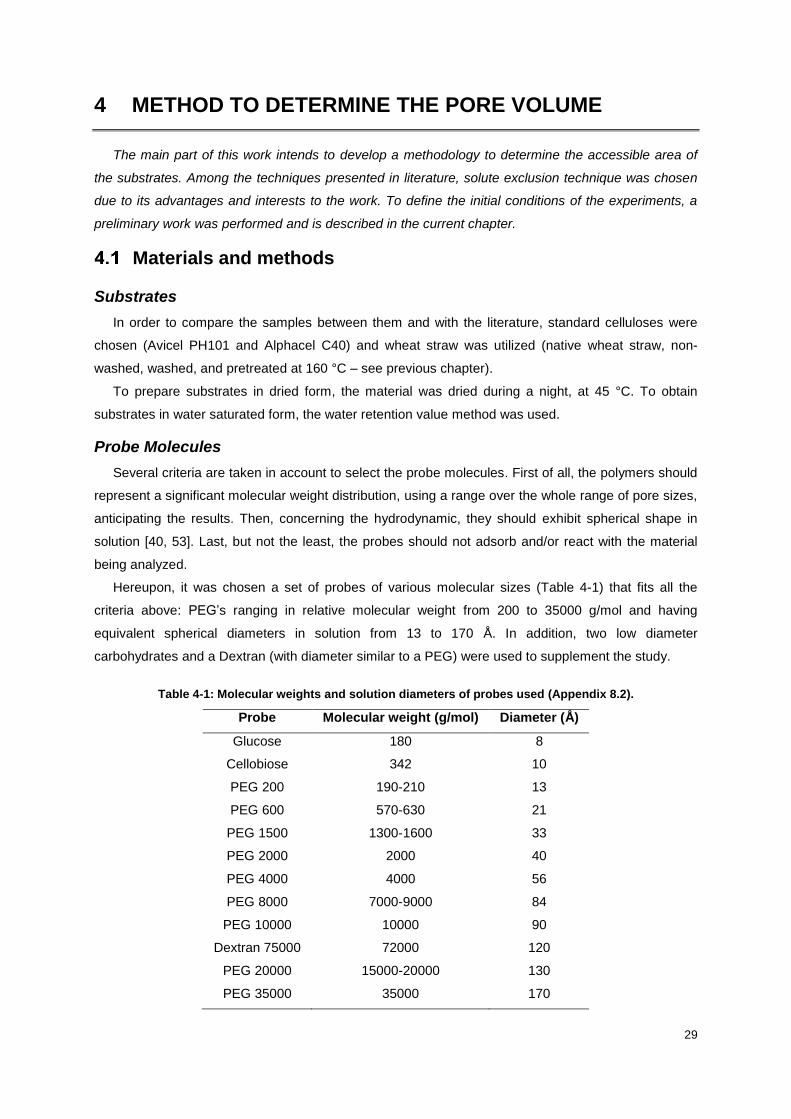
29

4 METHOD TO DETERMINE THE PORE VOLUME

The main part of this work intends to develop a methodology to determine the accessible area of

the substrates. Among the techniques presented in literature, solute exclusion technique was chosen

due to its advantages and interests to the work. To define the initial conditions of the experiments, a

preliminary work was performed and is described in the current chapter.

Materials and methods

Substrates

In order to compare the samples between them and with the literature, standard celluloses were

chosen (Avicel PH101 and Alphacel C40) and wheat straw was utilized (native wheat straw, non-

washed, washed, and pretreated at 160 °C – see previous chapter).

To prepare substrates in dried form, the material was dried during a night, at 45 °C. To obtain

substrates in water saturated form, the water retention value method was used.

Probe Molecules

Several criteria are taken in account to select the probe molecules. First of all, the polymers should

represent a significant molecular weight distribution, using a range over the whole range of pore sizes,

anticipating the results. Then, concerning the hydrodynamic, they should exhibit spherical shape in

solution [40, 53]. Last, but not the least, the probes should not adsorb and/or react with the material

being analyzed.

Hereupon, it was chosen a set of probes of various molecular sizes (Table 4-1) that fits all the

criteria above: PEG’s ranging in relative molecular weight from 200 to 35000 g/mol and having

equivalent spherical diameters in solution from 13 to 170 Å. In addition, two low diameter

carbohydrates and a Dextran (with diameter similar to a PEG) were used to supplement the study.

Table 4-1: Molecular weights and solution diameters of probes used (Appendix 8.2).

Probe Molecular weight (g/mol) Diameter (Å)

Glucose 180 8

Cellobiose 342 10

PEG 200 190-210 13

PEG 600 570-630 21

PEG 1500 1300-1600 33

PEG 2000 2000 40

PEG 4000 4000 56

PEG 8000 7000-9000 84

PEG 10000 10000 90

Dextran 75000 72000 120

PEG 20000 15000-20000 130

PEG 35000 35000 170

30

Methodology for substrate in saturated form

The first experiments were performed using a previously saturated substrate, as described in the

literature. The protocol consisted in the following sequence (Figure 4-1):

a) Saturation of the substrate in water by water retention value method;

b) Preparation of probe solutions;

c) Mixing of 1 g of saturated substrate with 10 mL of probe solution 1 %w/v – orbital shaking

during 3 h, at ambient temperature;

d) Decantation during 1 h and removal of exceeding solution;

e) Centrifugation of remaining mixture, during 30 min, at 3000 rpm and recovering of

supernatants to analyze;

f) Determination of dry matter content.

Figure 4-1: Scheme of the methodology for substrate in saturated form.

Water retention value method – WRV

This method is a useful reference to evaluate the performance of cellulosic materials relative to

moisture behavior [54, 55]: it measures the water retained by a material after centrifuging under

standard conditions.

The water retention value, WRV, is defined as the ratio of water contained in the sample after

centrifuging, at a certain force and time, relative to the dry weight of the sample, and is given by:

WRV(g/g) =Wwet − Wdry

Wwet

Equation 4-1

where Wwet is the weight of the sample after centrifuging and Wdry is the absolute dry weight of the

sample [54, 56].

The norm TAPPI UM 256 was used as reference to establish the operating conditions for this

methodology. So, to measure the WRV, the substrate was first put in contact with water during a night

31

under magnetic agitation. After, one hour decantation was done and then the excess of water was

removed with a syringe and the solid was recovered into a centrifugation tube. The centrifugation

occurred at 3000 rpm, during 30 min and the solid was recovered and weighted immediately. To

determine the dry weight, the solid stayed in the oven, at 45 °C, during a night and was weighted in

the end, and Equation 4-1 was employed.

Preliminary results

The factors that may influence WRV measurements include sample weights, centrifugal time and

force, pore size of filters used, and cellulosic particle sizes [54]. So, to verify the repeatability of the

results, step a) was particularly studied using the two standard celluloses (Avicel PH101 and Alphacel

C40) under the conditions described below – Table 4-2. Then, in order to perform this step, for

samples of each cellulose were prepared: three flasks with one gram of substrate each one, and a

fourth flask with five grams of substrate. To each flask were added 100 mL of water.

Table 4-2: Initial conditions of substrates to water retention value method.

ID Avicel PH101 Alphacel C40

ms (g) 1 (x3) 5 1 (x3) 5

water (mL) 100 100

In the assay with Avicel, the decantation was performed and no clearly separation occurred

(particles in suspension were observed). The experiment was repeated three times in these conditions

and one time with 6 h decantation, always with the same observation. For Alphacel a visible

decantation occurred at each time.

Then, six different samples were obtained from the four initial flasks: three samples were prepared,

one from each flask with 1 g ms (Set A), and the other were three obtained from the fourth flask (Set

B). This intended to verify if there is an influence in preparation of WRV method, regarding the sample

weights.

To determine the WRV, the saturated substrates were put into six different aluminum cups

(approximately 1 g) and transferred to the oven, at 45 °C, in order to determine also the ideal time of

drying.

As can be seen in Figure 4-2 and Figure 4-3, for both substrates, 2 or 3 hours is the minimum

period sufficient to get a material completely dried. This conclusion reduces drastically the time of the

experiment since only 3 hours are required for these substrates, instead of one night, as reported in

literature. However, maybe this time depends on the nature of the substrate.

Regarding the mass of initial substrate, there is no apparent difference in using 1 g or 5 g to

produce saturated substrate (Appendix 8.3). However, this sentence is contradictory when standard

deviation is included in the results: the values obtained from the same initial solution (Set B) produce a

more consistent set of samples, presenting an evident lower error.

Comparing the fiber size of the substrates (Avicel PH101 – 50 m and Alphacel C40 – 120 m),

there are no significant conclusion that can be made.

32

Figure 4-2: Evolution of mass substrate during drying, for Avicel PH101 (Table 8-4, Appendix 8.3).

Figure 4-3: Evolution of mass substrate during drying, for Alphacel C40 (Table 8-6, Appendix 8.3).

Another important point concerns the filters used during centrifugation. Sometimes holes were

found after centrifugation with no apparent reason. Factors that contribute for this can be the force of

centrifugation or the quantity of sample. Actually, this problem was found only for the 5 g samples,

which leads to conclude that this could be the cause of the holes. To solve this, an equilibrium

between the mass of sample and force of centrifugation should be done, for example, reducing the

force for heavy samples. However, the time of centrifugation maybe should be high to compensate. A

simply solution will be to reduce the mass of sample to centrifuge.

In the experiments, the filters used present blank color. When the substrate in study has the same

color as the filter, during the transfer of the matter to the cup, particles of filter can be dragged. This

could have repercussions in the final results, so the use of filters with a different color is proposed.

0.4

0.6

0.8

1.0

1.2

1.4

0 1 2 3 4 5 6

ma

ss

of

su

bs

trate

(g

)

time (h)

Set A

Set B

0.4

0.6

0.8

1.0

1.2

1.4

0 1 2 3 4 5 6

ma

ss

of

su

bs

tra

te (

g)

time (h)

Set A

Set B

33

Figure 4-4: Results from determination of WRV for Avicel PH101 (Table 8-7, Appendix 8.3).

Figure 4-5: Results from determination of WRV for Alphacel C40 (Table 8-8, Appendix 8.3).

Lastly, the WRV was determined and represented graphically (Figure 4-4 and Figure 4-5), being

1.01±0.19 g/g for Avicel and 0.73±0.02 g/g for Alphacel, with a confidence interval of 95%.

With these results the repeatability for the second substrate is validated, but not for the first one. At

this point, Alphacel was chosen to do the assays with the proposed methodology.

Methodology for substrate in dried form

For the second type of experiments, the samples were previously dried and this procedure is not

described in literature. So, an adaptation of the method using a substrate in saturated form was done,

following the next steps (Figure 4-6):

a) Drying of the substrate in oven by night, at 45 °C;

b) Preparation of probe solutions;

c) Mixing of 1 g of dried substrate with 10 mL of probe solution 1 %w/v – using orbital shaking

during 3 h, at ambient temperature;

d) Decantation during 1 h and removal of exceeding solution;

e) Recovering of remaining solution to analyze.

0.6

0.8

1.0

1.2

1 2 3 4 5 6

WR

V (

g/g

)

ID sample

0.68

0.72

0.76

0.80

1 2 3 4 5 6

WR

V (

g/g

)

ID sample

34

Figure 4-6: Scheme of the methodology for substrate in dried form.

Preliminary results

Once Alphacel demonstrated to be a more adequate substrate to practice the experiments, it was

also used in dried form methodology. A first series of trials was done to observe the main experimental

barriers and find a solution for them.

Concerning the substrate drying, due to the results obtained for the other methodology, it was clear

that three hours of drying were sufficient. Even less it will be acceptable, since the substrate in this

case is not saturated, it contains only the water from the air (near 4 %w/w).

Instead of the orbital shaking, as Gama et al. refer, a magnetic agitation was performed since the

first option did not allow the mixture of the substrate with the probe solution.

Probe solutions analysis

In order to determine the concentration of probe in the final solutions, a refractometer Anton Paar:

RXA170 was used – Figure 4-7.

For a known concentration solution in the begging, the refractive index of the final solution was

determined and then converted to concentration using calibration curves.

Figure 4-7: Refractometer used to measure the refractive index of solutions.

measuring chamber

results reader

35

To avoid interferences in the results, a syringe coupled to a 0.45 m filter (Figure 4-8) was used to

ensure that no fragments were transferred to the measuring chamber.

Figure 4-8: Sample recovered after decantation and prepared to analyze in refractometer.

Due to the few quantity of supernatant obtained in the end of the experiments, the samples were

measured only one time. For the calibration curves, the solutions were prepared in a quantity sufficient

to obtain at least four measurements for each concentration.

Calibration of the refractometer

The aim of the calibration experiments was to define an equation that relates the refractive index

measurement with concentration of probe. Then, the repeatability and reproducibility of the

measurements were also tested. So, as said above, each refractive index was measured four times,

for each concentration, for the different probe molecules. Also, new solutions were prepared for each

experiment.

To convert the refractive index measurements in concentration of probe, the linear correlation

obtained for each series of data was used:

Cf =nDsample − b

m Equation 4-2

where m is the slope of the calibration curve and b is the interception with the yy axis and

corresponds to a solution with a null concentration in probe (so, water).

Calibration curves were performed using an adequate concentration range, depending on the

substrate used (between 1 %w/v and 3 %w/v). As an example, the values measured for PEG 35000

and PEG 200 are presented and discussed.


y = 0.00135x + 1.33289R² = 0.9999

1.3340

1.3350

1.3360

1.3370

1.0 1.5 2.0 2.5 3.0

nD

concentration (%w/v)

syringe

filter

36


Regarding previous figures, it was possible to verify a good linear correlation between refractive

index and concentration for PEG 35000 and the equation is the same for different days. This proves

that the assays with PEG 35000 are repeatable, as well, reproducible. But then, when other probes

were tested, a different conclusion can be made. For example, for PEG 200:

Figure 4-11: Evolution of calibration curves for PEG 200 (between 28/05/2015 and 15/07/2015).

Table 4-3: Linear correlations between refractive index and concentration for PEG 200 (Figure 4-11).

ID Date Linear correlation R2

15/07/2015 y = 0.00132x + 1.33274 0.9996

10/06/2015 y = 0.00133x + 1.33272 0.9985

28/05/2015 y = 0.00130x + 1.33272 0.9970

29/05/0215 y = 0.00126x + 1.33276 0.9975

y = 0.00135x + 1.33289R² = 1

1.3340

1.3350

1.3360

1.3370

1.0 1.5 2.0 2.5 3.0

nD


1.3340

1.3341

1.3342

1.3343

1.3344

1 1.05 1.1 1.15 1.2 1.25

nD


37

As can be seen in Table 4-3, the sensibility for this probe is very similar (same slope). Also the

coefficient R² demonstrates the good repeatability of the data obtained. Nevertheless, regarding

Figure 4-11 it is clear that there are some variations. These results are no negligible for concentration

determination.

So, two parameters are significant when calibration is performed: the probe used and the evolution

of the measurements in time. The first one is evident in the example above and, in general, this

variation will be related with experimental errors (such as preparation of the probe solution). Regarding

the evolution in time, for the same probe, it makes us to conclude that calibration should be done at

each experiment in order to avoid errors in calculations.

Then, after all calibrations, can be concluded that:

the sensibility of the method to the probes is similar (Figure 4-12);

the calibration curves should be done at each experiment;

about the number of measurements, can be settled that one or two measurements will be

sufficient due to the good repeatability observed.

All the linear correlations obtained between refractive index and concentration for all the probe

molecules are presented in Appendix 8.4.

38

Figure 4-12: Examples of calibration curves for the different probes.

PEG35000

PEG200

Glucose

Cellobiose

1.3340

1.3350

1.3360

1.3370

1.0 1.5 2.0 2.5 3.0

nD


PEG35000 PEG20000 PEG8000 PEG4000 PEG1500 PEG600 PEG200 Glucose Cellobiose

39

5 RESULTS OF SUBSTRATE POROSITY

For the methodologies described and the equations established, the accessible pore volume to

probe molecules into the substrate was determined. Following this, the reproducibility of the procedure

was evaluated and discussed for the different substrates. This section intends to explore the results

obtained, as well discuss about them.

Determination of pore volume

Saturated substrate method

In this method, two phases can be distinguished: the beginning of the experiment (t0), where the

concentration in solution, Ci, is assumed to be the same concentration of the probe – Equation 5-1,

and a second time (t), when the concentration will be different from the initial, Ceq, if the probe enters

inside the pores – Equation 5-2.

t0 ⇒ nprobe = Vsol ∙ Ci Equation 5-1

t ⇒ nprobe = (Vsol + Vp) ∙ Ceq Equation 5-2

By mass balance, the pore volume, Vp, can be determined by:

Vp =Vsol ∙ (Ci − Ceq)

Ceq

⇔ Ceq = Ci ∙Vsol

(Vsol + Vp) Equation 5-3

As said before, the substrate is saturated. Consequently, if the probe goes into the pores, the

concentration of the final solution, Ceq, is decreased by dilution.

In order to use the saturated substrate method, it is appropriate to determine the water retention

value. Subsequently, at each experiment, this value was calculated. As can be seen in Figure 5-1, the

method is consistent when Alphacel is used, presenting a value of 0.64±0.02 g/g.

Figure 5-1: Distribution of values for water retention method, for Alphacel (Table 8-10, Appendix 8.5).

0.60

0.62

0.64

0.66

0.68

0.70

1 6 11 16

WR

V (

g/g

)

ID

SE01 SE02 SE03 SE04 SE10

40

So, from Equation 5-3, it is expected to obtain a final concentration lower (if probe penetrates) or

equal (if nothing happens) to the initial solution.

Regarding the final concentrations for these trials (Table 8-10, Appendix 8.5) using this method the

porous volume determined is often negative. This result is obtained whenever the final concentration is

higher than the concentration of initial solution:

Ceq ≥ Ci ⇒ (Ci − Ceq) ≤ 0 ⇒ Vp ≤ 0 Equation 5-4

Figure 5-2: Calibration curve and results for experiment SE02 (Table 8-10, Appendix 8.5).

Taking the experiment on Figure 5-2 as example, the relation described by Equation 5-4 is shown

and then pore volume is negative.

The first issue that can be discussed is the possible existence of soluble compounds or

contaminants in the substrate. Chen and his co-workers [57] report a mass percentage of water-

soluble materials varied from 14 to 27% for corn samples. Among these soluble, monomeric sugars

(primarily glucose) were found to be the predominant water-soluble components. These compounds

can significantly affect the refractive index measurements. Following this, it is reported in literature [19,

57] that the removal of soluble contaminants and fine cellulose particles should be done, since they

are a source of interference during the refractometric measurements.

Additionally, sample preparation can also add significant deviation in the results. For example,

during centrifugation can occurs water removal from the pores, due to the cellulose packing [19]. After,

when samples are prepared for mixing with the probe solution, evaporation of water from the saturated

substrate can also occur.

Therefore, the cause of these unexpected results was not clear. For this reason, it was decided to

discard this first methodology.

Dried substrate method

To determine the porous volume with this second methodology, it was necessary to make

assumptions and do the calculations in two different parts.

When a dried substrate is used, after the contact with the probe solution, two situations can occur:

only water penetrates into the pores or the solution of probe penetrates into the pores, depending on

the size diameter of the probe.

41

Figure 5-3: Scheme of a porous substrate and penetration of molecules.

Following the previous reasoning, by using several probes of different sizes, it will be possible to

obtain a distribution of pore sizes. By assumption, once water is a small molecule (bond O-H lengths

approximately 1 Å [58])., then enters on the total volume of pores, Vp, However, the probe, depending

on its size, penetrates only on the volume where the pore diameter is higher than its diameter, Va (as

schematized on Figure 5-3). The difference between the total pore volume and the accessible volume

is defined as the inaccessible volume, Vi.

Furthermore, it is assumed that the probe concentration into the pores is the same of the solution

that surrounds the substrate.

Hereupon, the following equations were established:

nprobe = Vsol,i ∙ Ci Equation 5-5

nprobe = (Va + Ve) ∙ Cf Equation 5-6

Vp = Va + Vi Equation 5-7

Vsol,i = Ve + Vp Equation 5-8

This equation system cannot be solved by itself. In this way, some hypotheses were assumed in

order to determine the unknown variables.

Then, for the probe molecule with higher diameter (PEG 35000), it was assumed that this probe is

too big to penetrate inside the pores (even the biggest ones) and the accessible pore volume is

defined as equals to zero. Doing this, it was possible to determine the external volume, Ve, with

Equation 5-6. This value will be constant for all the experiments with the probes of smaller diameter

than PEG 35000. After, the total pore volume can be also determined from Equation 5-8, and, in this

case, it corresponds to the inaccessible pore volume to the probe.

On the other side, for the remaining molecules the inaccessible volume can be easily estimated

using Equation 5-9, that results from the rearranging of the equations below.

Vi =Vsol,i ∙ (Cf − Ci)

Cf

Equation 5-9

At this time, all the parameters were known, therefore the accessible volume was estimated once

the porous volume was assumed as constant.

Knowing these parameters, the pore volume was estimated for all the substrates (Table 5-1) and

the distribution is discussed in the next section.

42

Table 5-1: Exterior and maximal pore volume determined for the substrates.

Substrate 𝐕𝐞 (mL/g mds) 𝐕𝐩 (mL/g mds) Reference

Alphacel 9.17±0.03 0.77±0.04 Table 8-11

non-washed native wheat straw 9.81±0.04 0.18±0.05 Table 8-16

washed native wheat straw 9.23±0.04 0.72±0.04 Table 8-19

washed pretreated wheat straw 9.25±0.01 0.75±0.00 Table 8-20

It was expected an increment on porous volume in the order described in Figure 5-4. Regarding the

results, this relationship was verified when non-washed native wheat straw is compared with the

washed, as well, the washed pretreated. However, the value for non-washed could be probably wrong

due to the uncertainty associated to the measurements and calculations.

Then, comparing washed native with washed pretreated, the result is controversial. The porous

volume is the same if standard deviation is taken in account. One reason for this can be the difficulty

to delete the part of the soluble compounds, which still remain after washing, in the refractive index

measurement. Another cause can be related with the pretreatment effects. In this step, some pores

can be created with the treatment, but also other ones can be destroyed [59, 60]. This can result in

larger pores, or, on the other side, irreversible collapse of pores. So, even if porosity value does not

change, new pores with different sizes can be created.

Figure 5-4: Expected increasing in accessible porous volume by type of substrate.

The total pore volume determined here corresponds to the fiber saturation point, FSP. As said

previously, this value corresponds to the plateau of the distribution curve (Figure 2-16). In this work

were obtained results of the same order of magnitude than these obtained by other authors (Table

5-2).

For Alphacel, the standard cellulose, it was found a value near to Avicel PH 101. This commercial

product was studied by Gama and his-co-workers. However, it is important to retain that Gama used a

protocol with the substrate in saturated form. In the present work, dried substrate methodology was

applied.

For substrates in native form, it is not clear in literature if they were previously washed. Comparing

with the result obtained in this work, the value obtained by Thompson [24] is similar. Nevertheless, the

substrate is not the same, consequently, any conclusion can be done. Regarding other studies [59],

also the substrates used are not the same that the one used in this study. Further, the value obtained

is quite different from wheat straw (same order of magnitude).

Lastly, to the substrate pretreated at 160 °C and washed, literature refers a similar value but for

mixed hardwood. This substrate was pretreated under similar conditions than wheat straw.

non-washed

native

washed

native

pretreated

washed

+𝐕𝐩

43

Furthermore, it can be noticed that there are no significant difference in FSP between the native mixed

hardwood sample and the pretreated one. The same evidence occurred in the present study.

Table 5-2: Fiber saturation point by solute exclusion technique, from literature.

Substrate Pretreatment FSP (mL/g) Reference

Avicel PH 101 0.70

[19]

Sigmacell 100 1.09

Whatman CF 11 0.42

Crystalline cotton 0.93

Amorphous cotton 1.35

mixed hardwood

0.76

[24]

180 °C, 1 %w/w H2SO4 0.77

200 °C, 1 %w/w H2SO4 1.06

220 °C, 1 %w/w H2SO4 1.33

mixed hardwood 0.51

[59] 200 °C, 1 %w/w acid 0.92

white pine 0.49

200 °C, 1 %w/w acid 0.71

Solka Floc BW 300 1.6 [53]

Pore volume distribution

As said before, the measurements of refractive index for each sample were done only one time,

due to the restrict quantity of sample available. Then, each point was obtained from a series of four

samples for each different probe experiment – Figure 5-5. Thus, the experimental errors were

calculated as the relative standard deviation of the data considered for calculations (with a 98%

confidence interval) and are shown by the error bars in the figures along this chapter. The fifth sample

was prepared adding only water to the substrate. This sample served as control, allowing the

subtraction of possible soluble compounds that interferes in the refractive index measurements.

Figure 5-5: Example of a series of samples in a trial.

blank

sample

samples

in a trial

44

For the series of probes used and for the different substrates, it was expected to obtain a set of

points similar to what is shown in the next figure, obtained from previous studies:

Figure 5-6: Pore volume distribution for pulp fibers exposed to different conditions [40].

This data reveals that there is a plateau corresponding to a maximum inaccessible volume to the

probe or the fiber saturation point (signed on Figure 5-6 with an arrow). Also occurs a decrease of the

volume as function of the probe molecular diameter. This looks like to be independent from the

methodology or pretreatment applied to the substrate [40] – Table 5-3.

Table 5-3: Fiber saturation point from different pretreatments.

Substrate Type Pretreatment FSP (mL/g) Reference

wheat straw acid 0.72

this work 160 °C, 1 %w/w H2SO4 0.75

mixed hardwood acid

0.76

[16]

180 °C, 1 %w/w H2SO4 0.77

200 °C, 1 %w/w H2SO4 1.06

220 °C, 1 %w/w H2SO4 1.33

mixed hardwood alkaline

0.5 h, H2O2 0.87

[33] 5 h, H2O2 1.43

19 h, H2O2 1.41

mixed hardwood organosolv

10 % ethylenediamine 1.08

[33] 50 % ethylenediamine 0.96

70 % ethylenediamine 1.47

45

So, from substrate to substrate, this pore volume distribution, as function of pore diameter, can be

defined by two variables: the value of the plateau or fiber saturation point and a constant. The plateau

will indicate the total porous volume of the substrate. The constant will define the behavior of the curve

and will depend on the substrate used.

Following this reasoning, an equation was proposed with the intuit of modeling the experimental

results obtained in this work:

Vi = Vi,max(1 − e−kD) Equation 5-10

where Vi,max is the value of the plateau and is determined by using the higher molecular diameter

probe, D, when accessible volume is null. The constant, k, was determined using the minimum square

error method. Both these parameters are specific of each substrate.

The type of pores in the substrates was also determined (Table 5-4). This study reveals the type of

pores that exist, but says nothing about their location in the cell wall.

Table 5-4: Types of porosity in solids [61].

Type Pore size (nm)

microporous < 2

mesoporous 2 – 50

macropores > 50

To remind, the higher size diameter of probe molecule used in this work corresponds to PEG35000

(170 Å). By this, nothing can be concluded about the macroporosity of the substrates (when pore size

is higher than 500 Å) – example in Figure 5-7.

In summary, the type of porosity defined in this study is valid on the range of probe molecular sizes

studied (between 8 and 170 Å). Additionally, to determine the position of that pores, another type of

characterization method should be used (such as scanning electron microscopy).

Figure 5-7: Scheme representative of different levels of porosity.

To introduce the results, a briefly explanation is done about how the points were obtained. For this,

the example of Alphacel is used.

46

Alphacel C40

To obtain the first point, the larger molecule size diameter was used (PEG 20000, in this case). By

this, it was assumed that this molecule will not enter the pores and, consequently, the accessible

volume will be zero. In this way, the total porous volume of the substrate was determined.

To do that, the concentration of final solution was measured by refractometry (one measurement

by sample). Using the calibration curve, the refractive index measurement is converted in

concentration of probe. Finally, the exterior volume was determined using Equation 5-6, as well, the

total porous volume, using Equation 5-8. The final volume value was determined by the average of the

four measurements and standard deviation was also calculated.

Table 5-5: Example of exterior and total porous volume determination, for Alphacel (Table 8-11).

Sample mds (g) nD Cf (g/100mL) Ve (mL) 𝐕𝐩 (mL/g mds)

1 1.0131 1.33435 1.10 9.15 0.85

2 1.0136 1.33433 1.08 9.27 0.73

3 1.0008 1.33434 1.09 9.21 0.79

4 1.0031 1.33434 1.09 9.21 0.79

AV±SD – – – 9.17±0.03 0.77±0.04

As can be noted on Table 5-5, an error of 0.00001% on refractive index will reproduce an error of

0.1% on the value of final concentration. Furthermore, this will represent an error of almost 20% in the

total porous volume. The last value is tremendous and certainly will affect the final distribution.

At this point, the first point was obtained. In order to obtain the other points, progressively smaller

molecules were used. By this, the accessible volume to the probes was calculated using Equation 5-6,

once the external volume is constant for the substrate.

Finally, the model equation proposed can be employed and the pore size distribution was obtained.

The data for this substrate are clearly repeatable (Figure 5-8) and Equation 5-11 reflects these results.

Figure 5-8: Pore volume distribution for Alphacel (Table 8-21, Appendix 8.10).

Vi = (0.77 ± 0.04)(1 − e−0.05D) Equation 5-11

0.0

0.2

0.4

0.6

0.8

1.0

0 50 100 150 200

Inaccessib

le p

ore

vo

lum

e

(mL

/g m

ds)

diameter (Å)

47

As can be noticed, the data reveal that the pores are almost impermeable to probes with a

diameter above 50 Å. So, it can be concluded that exists micro and mesoporosity in this substrate, in

the studied range of diameters.

Another standard cellulose was tried by Gama and his co-workers, named Avicel, and the same

evidences were verified – Figure 5-10. To clearly compare the data obtained in this work with these

results, the accessible volume as function of diameter is represented on Figure 5-9:


Figure 5-10: Pore volume distribution of celluloses (Table 5-2) [19].

For the five substrates studied by Gama, it was observed a fiber saturation point that correspond to

probe molecules with a 50 Å diameter or higher.

In particular, regarding Avicel, it was found a behavior of distribution similar to Alphacel. However,

it is important to retain that Gama and his co-workers worked with a saturated substrate. In the present

work, the dried substrate methodology is used.

To conclude, the dried substrate methodology was validated for Alphacel.

0.0

0.2

0.4

0.6

0.8

1.0

0 50 100 150 200

Ac

ce

ss

ible

po

re v

olu

me

(m

L/g

md

s)

diameter (Å)

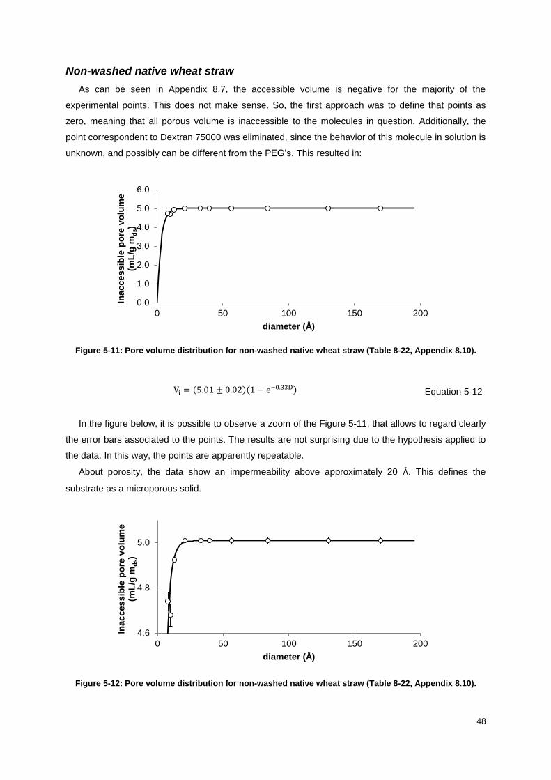
48

Non-washed native wheat straw

As can be seen in Appendix 8.7, the accessible volume is negative for the majority of the

experimental points. This does not make sense. So, the first approach was to define that points as

zero, meaning that all porous volume is inaccessible to the molecules in question. Additionally, the

point correspondent to Dextran 75000 was eliminated, since the behavior of this molecule in solution is

unknown, and possibly can be different from the PEG’s. This resulted in:


Vi = (5.01 ± 0.02)(1 − e−0.33D) Equation 5-12

In the figure below, it is possible to observe a zoom of the Figure 5-11, that allows to regard clearly

the error bars associated to the points. The results are not surprising due to the hypothesis applied to

the data. In this way, the points are apparently repeatable.

About porosity, the data show an impermeability above approximately 20 Å. This defines the

substrate as a microporous solid.


0.0

1.0

2.0

3.0

4.0

5.0

6.0

0 50 100 150 200

Ina

ccessib

le p

ore

vo

lum

e

(mL

/g m

ds)

diameter (Å)

4.6

4.8

5.0

0 50 100 150 200

Inaccessib

le p

ore

vo

lum

e

(mL

/g m

ds)

diameter (Å)

49

As said earlier, a blank sample was prepared and analyzed at each trial. From the experimental

point of view, this sample containing only water instead of probe solution was prepared as control and

is advised by some authors [24, 42]. The reason for this is to allow deducting the contributions of water

soluble extractives, or other contaminants, in the refractive index measurements.

Thus, for this substrate, final concentrations were corrected for the possible existence of

contaminants (directly deducted on refractive index measurements).

The correction was done by subtracting out the specific reading from blank to wheat straw sample.

For this, the average of all measurements for the blanks was calculated. Then, the refractive index

correspondent to the contribution of the soluble can be determined through:

∆soluble = nDblank,AV − nDwater Equation 5-13

where nDblank,AV and nDwater are 1.33420 and 1.33286, respectively. As can be noticed by the

value obtained, there is a strong contribution of the soluble components.

Likewise, it is possible to determine the variation associated to the presence of probe:

∆probe = nDsample − nDblank,AV Equation 5-14

where nDsample depends on the sample and probe solution.

To finish, the corrected refractive index can be calculated by:

nD′ = ∆probe − nDwater Equation 5-15

This equations were then applied and a completely different set of results was obtained, as can be

seen in the next figure:

Figure 5-13: Pore volume distribution for non-washed native wheat straw, with refractive index correction – all points included (Table 8-23, Appendix 8.10).

The new data obtained look like as expected. In a calculation of this type, there is a subtraction of

two big numbers, with a small deviation associated to each one. The result of this deduction is a small

number, with a deviation associated of its order of magnitude.

To model these results, the point correspondent to PEG 2000 was eliminated. Also, it was used the

same hypothesis than the one applied for Alphacel: once the accessible or inaccessible volume is

negative, then it turns zero. Then, for the three smallest diameters, there are not accessible volume. In

-1.5

-1.0

-0.5

0.0

0.5

1.0

0 50 100 150 200

Inaccessib

le p

ore

vo

lum

e (

mL

/g m

ds)

diameter (Å)

50

addition, a reasoning was done concerning the measured concentrations: the points with higher

deviation between them were eliminated. These data can be extensively consulted in Appendix 8.7.

Figure 5-14: Pore volume distribution for non-washed native wheat straw, with refractive index correction. (Table 8-23, Appendix 8.10)

Vi = (0.18 ± 0.05)(1 − e−0.01D) Equation 5-16

Therefore, the new result is traduced by Figure 5-14. As explained, the points with no error bars

represent an apparent repeatability, since they result from the elimination of points in order to optimize

them. This was done with a logical reasoning due to the knowledge acquired with Alphacel

experiments.

To conclude, the results with non-washed native wheat straw are not exploitable. Too much

hypotheses and approximations were applied. This seriously affected the results. Moreover, the final

result is not similar to literature data (Table 5-3).

At this point of the work, the question of the possible existence of soluble components was taken in

account. Once the mathematically correction did not result in exploitable data, another solution was

established, acting directly on the substrate preparation. This introduces the next section, where the

native wheat straw was previously washed.

Washed native wheat straw

To confirm the hypothesis that the soluble compounds affect tremendously the refractive index

measurements, the native wheat straw was previously washed with water. Due to the time available

for the trials, only three points were obtained.

The quantity of soluble was then determined using Equation 5-13. Concerning Table 5-6 it is

perfectly visible that the quantity of soluble decreases drastically with the washing. Furthermore, the

results are measured in the refractive index apparatus. As can be seen, the order of magnitude of the

contribution of these compounds is significant for non-washed wheat straw when compared with

washed. By this, the results for this substrate were extremely affected. Subsequently, the contribution

of soluble was also deducted to the results obtained for washed native wheat straw.

0.00

0.05

0.10

0.15

0.20

0.25

0 50 100 150 200

Inaccessib

le p

ore

vo

lum

e

(mL

/g m

ds)

diameter (Å)

51

Table 5-6: Contribution of soluble components for refractive index measurements.

Substrate ∆𝐬𝐨𝐥𝐮𝐛𝐥𝐞

native non-washed 0.00134

native washed 0.00014

Figure 5-15 : Pore volume distribution for washed native wheat straw (Table 8-24, Appendix 8.10).

Vi = (1.51 ± 0.03)(1 − e−0.13D) Equation 5-17

Figure 5-16: Pore volume distribution for washed native wheat straw, with refractive index correction (Table 8-25, Appendix 8.10).

Vi = (0.72 ± 0.04)(1 − e−0.04D) Equation 5-18

Concerning these figures (Figure 5-15 and Figure 5-16), the differences are evident. The first thing

that can be noted is the difference in the fiber saturation point value. By subtracting the contribution of

soluble, the plateau decreases from 1.5 to 0.7 mL/g mds, half of the first value obtained. It can be firstly

0.0

0.5

1.0

1.5

0 50 100 150 200

Ina

cc

es

sib

le p

ore

vo

lum

e

(mL

/g m

ds)

diameter (Å)

0.0

0.2

0.4

0.6

0.8

0 50 100 150 200

Inaccessib

le p

ore

vo

lum

e

(mL

/g m

ds)

diameter (Å)

52

conclude that this contribution should be subtracted. Afterwards, if the soluble are not deducted, the

distribution obtained will correspond to a pore size value higher than the real one.

Regarding porosity, a conclusion can be made, based on the behavior of model equation

proposed. A fiber saturation point was encountered at 0.7 mL/g mds, since a size diameter of

approximately 50 Å. This indicates the presence of micro and mesopores.

Comparing the corrected data of washed native wheat straw with non-washed native wheat straw.

The fiber saturation point is completely different. Actually, the total pore volume for the washed sample

is approximately four times higher than the non-washed.

Due to this evidence, the non-washed data were not considered to make conclusions. Excepting

the evidence about the soluble compounds. With this, the existence of soluble can be corroborated

and it should be taking in account.

Washed and pretreated wheat straw

The other product tried was a sample pretreated with acid, at 160 oC. After pretreatment, the

sample was subjected to a washing in order to eliminate some contaminants.

Due to limited time, only three experiments were performed using as probes PEG 35000, PEG

20000 and glucose. Among these, the results obtained for glucose were not considered in

calculations.

Figure 5-17: Pore volume distribution for washed and pretreated wheat straw (Table 8-26, Appendix 8.10).

Vi = (0.75 ± 0.00)(1 − e−0.02D) Equation 5-19

As can be seen on Figure 5-17, two points did not allow to make conclusions. Additionally, the

model equation cannot describe this distribution due to this absent of data. A value for the fiber

saturation was obtained, nevertheless, it is not clear if the total porous volume corresponds to that

value. Regarding the same figure, it is not observed the plateau. Can be supposed that the plateau will

be at high value, as result of the pretreatment. Also, no one conclusion should be made about the type

of porosity. Accordingly, at this point, more study is required on pretreated sample.

0.0

0.2

0.4

0.6

0.8

0 50 100 150 200

Inaccessib

le p

ore

vo

lum

e

(mL

/g m

ds)

diameter (Å)

53

Conclusion

At this moment is time to make a summary of all data obtained until now. Once the data for non-

washed native wheat straw was found to be not exploitable, it is not represented in this section. Then,

the results obtained were put all in the same figure and represented using a logarithmic scale:

Figure 5-18: Pore volume distribution for Alphacel and different wheat straw products.

Once there are not published studies using this new approach of solute exclusion, as well, there

are few information on wheat straw, only a preliminary comparison can be made. Recalling Stone and

Scalan work, can be noted on Figure 5-19 that the behavior of data from the present work is

comparable with their study on pulp fibers dried and reswollen.

Figure 5-19: Pore volume distribution for pulp fibers – zoom of Figure 5-6 [40].

0.0

0.2

0.4

0.6

0.8

1 10 100 1000

Inaccessib

le p

ore

vo

lum

e (

mL

/g m

ds)

diameter (Å)

alphacel

washed native

pretreated 160oC

54

Similarly to the same authors, in the current study, the plateau was observed between 0.6 and 0.8

mL/g mds. The behavior of the curve (defined by a constant) is also analogous, however, about this

none conclusion should be made, since that this behavior depends on the substrate used.

Determination of specific surface area

As previously referred, surface area available is an important parameter on enzymatic hydrolysis,

regarding the pretreatment method (section 2.3.2). Consequently, it is interesting to study the five

different samples pretreated in this work in order to compare them with native sample and to notice the

differences between them.

Though, the limitation of the applicability of this method should be retained: nitrogen adsorption

measurements provide specific surface area for a molecule that is 3200 times smaller than the

average cellulase [60]. Concerning the figure above, this affirmation turns completely clear. There, the

influence of probe size on the determination of available surface area is perceptible.

Figure 5-20: Schematic representation of the structural features of the cellulose particle surface [19].

Afterwards, this analysis was performed on the different substrates and the results can be seen on

Table 5-7. The specific surface area, SSABET, increases from the sample pretreated at 100 °C until the

sample pretreated at 180 °C. These results were predictable since it was expected an increment on

SSA with the severity of the pretreatment. Furthermore, the native sample has a SSA lower than the

other ones. Likewise, this relation was expected and translates the effectiveness of the pretreatment

on the increasing of the available surface area.

Table 5-7: Results of specific surface area from N2 gas adsorption, in this work.

Substrate ID Pretreatment SSABET (m2/g)

wheat straw

C0033 – 0.77

CR_1082L 100 °C, 20 min, 1 %w/w H2SO4 0.97

CR_1081L 120 °C, 20 min, 1 %w/w H2SO4 1.27

CR_1083L 140 °C, 20 min, 1 %w/w H2SO4 1.71

CR_1080L 160 °C, 20 min, 1 %w/w H2SO4 2.79

CR_1084L 180 °C, 20 min, 1 %w/w H2SO4 6.27

55

Some similar results on pretreated wheat straw were found in literature. In fact, the values reported

have the same order of magnitude than the ones achieved in this work even if the operating conditions

are not the same: different temperatures (between 120 and 190 °C) with different quantities of acid

(0.5 to 2 %w/w), as well, variable residence time (7 to 240 min). By this, the results are only coherent

for the higher temperatures.

Table 5-8: Specific surface area from literature, for wheat straw, by N2 gas adsorption.

Substrate Pretreatment SSABET (m2/g) Reference

wheat straw

– 3.3 [25] – 4.0

[62]

120 °C, 240 min, 1 %w/w H2SO4 5.7 140 °C, 25 min, 2 %w/w H2SO4 5.4 160 °C, 7 min, 1.5 %w/w H2SO4 5.5 170 °C, 10 min, 1 %w/w H2SO4 6.2 180 °C, 7 min, 0.5 %w/w H2SO4 7.1 190 °C, 10 min, 0.5 %w/w H2SO4 6.6

Summary and discussion

At this point, some considerations can be done. Using Alphacel, the results of size exclusion

analysis were reproducible and dried substrate methodology was validated. Regarding non-washed

and washed native wheat straw, it can be settled that the washing is significant in order to avoid

deviation on the results. For washed native wheat straw, as well, pretreated at 160 oC and washed, a

more complete study is required.

This section intends to make some general conclusions to summarize the data obtained and to

explain details that can considerably affect the experiments.

In the figure below is represented the accessible volume of untreated and pretreated corn stover,

as function of probe diameter proposed by Ishizawa et al. [42]. In parentheses are indicated the

cellulose digestibilities after seven days. The error bars represent the standard deviation of three

replicates.

Figure 5-21: Accessible pore volume of corn stover, measured by solute exclusion [42].

56

Ishizawa and his co-workers obtained the measurements of concentration of probe using an HPLC

apparatus equipped with a refractive index detector. Considering these results can be noted that the

error bars present a random and important deviation from sample to sample. This bad reproducibility

was found in the present study and is also encountered by these authors. This reinforces the

imprecision associated to a measurement of this type.

Due to this evidence, it is important to solve the problem of the measurements. So, in order to

improve the acquisition of data, a brainstorming was performed. The issue that seems to affect more

these results is the small gap between the initial and the final concentration of probe. Consequently, it

is needed to find a solution for this.

Using Equation 5-5 and Equation 5-6, the ratio between final and initial concentration of probe can

be obtained:

Cf

Ci

=Vsol,i

Va + Ve

Equation 5-20

As it is known, the volume of initial solution is already defined (Equation 5-7) and the porous

volume as well (Equation 5-8). By this, rearranging the equation, it results in:

Cf

Ci

=1

1 −Vi

Vsol,i⁄

Equation 5-21

where Vi is characteristic of the solid in study and can be expressed by:

Vi = εsolid × Vsolid Equation 5-22

where Vsolid is the volume of biomass and εsolid its porosity. Substituting this variable in Equation

5-21, the ratio of concentrations will be defined by:

Cf

Ci

=1

1 − εsolid ∙msolid

dsolid∙

1Vsol,i

Equation 5-23

The last equation represents the relation between the ratio of concentrations at the begging and at

the end of the experiment, with the variables of the trial. As can be noted on Table 5-9, it can be seen

that the final concentration can be very different regarding the substrate used. This concentration will

allow to determine the porous volume. Therefore, this measurement should be obtained accurately.

Table 5-9: Example of concentrations of probe (Appendix 8.6; Appendix 8.7).

Substrate Probe Ci (g/100mL) Cf (g/100mL)

Alphacel PEG 20000 1.00

1.10

Wheat straw 1.02

Regarding the same expression (Equation 5-23) it is evident that two parameters can be modified

from the experimental point of view in order to maximize the ratio of concentrations: the volume of the

probe solution, Vsol,i, and the mass of substrate used, msolid. Porosity and density will depend on the

substrate and cannot be modified.

57

Influence of the mass of substrate and the volume of probe

To evaluate the impact of the mass of substrate used, Equation 5-23 can be simplified:

Cf

Ci

=1

1 − K ∙ msolid

; K =εsolid

dsolid

∙1

Vsol,i

Equation 5-24

In this case, the influence of the quantity of solid is been evaluated, maintaining constant the

volume of probe solution. Supposing that the ratio between porosity and density it is one, than the

constant K will take the value of 0.1 g-1 (once the initial volume of solution is 10 mL).

Concerning this example and the results on Table 5-10, it is clear that an increase in solid mass will

allows the final concentration to increase. In this way, with the possibility of increasing the

concentration in the end, more precise results would be obtained.

Table 5-10: Influence of substrate quantity in final concentration of probe.

Increment 𝐊 ∙ 𝐦𝐬𝐨𝐥𝐢𝐝 𝟏 − 𝐊 ∙ 𝐦𝐬𝐨𝐥𝐢𝐝 𝟏

𝟏 − 𝐊 ∙ 𝐦𝐬𝐨𝐥𝐢𝐝

𝐂𝐟

2 ∙ msolid 2 0.8 1.25 ↑

6 ∙ msolid 6 0.4 2.50 ↑↑

8 ∙ msolid 8 0.2 5.00 ↑↑↑

10 ∙ msolid 10 0 - -

Nevertheless, it exists an asymptote in the increment of mass. As can be noted on Figure 5-22, at

certain point, that increasing does not make sense: thus, there is a limit to this parameter. Observing

Equation 5-23 it is perceptible that this asymptote corresponds to the point where the denominator of

the equation turns zero.

Figure 5-22: Influence of substrate quantity in final concentration of probe.

This behavior was expected. Once the mass of substrate is increased, the porous volume is also

increasing. By this, the final concentration of probe will be equal to the initial concentration or higher

than the initial concentration if not all the probe can enters the pores. Additionally, the quantity of

solution is fixed in 10 mL. In this case, if the quantity of substrate is being increased, the porous

volume is increasing as well. Consequently, this limit of concentration can happen before, since the

0

2

4

6

8

10

0 2 4 6 8 10 12

Cf(g

/100m

L)

msolid (g)

Ci

58

porous volume can equalize the volume of solution. In this situation, the final concentration will depend

totally on the probe size diameter: if the probe size is higher than all pores, than only water will

penetrate into the substrate; on the other hand if it is smaller than the porous diameter, the final

concentration will be zero. The last case is a limit case and should not be achieved because the

volume of solution will be higher than the porous volume available and the measurement will not be

correspondent to the reality.

Then, regarding Equation 5-23, it can be noted that reducing the volume in order to increase the

final concentration, is the same thing that increase the mass of substrate. By this, can be concluded

that the true parameter will be the ratio instead of the parameters by themselves. From a mathematical

point of view, if the mass of substrate and the volume of solution are considered as independent

parameters, it will results in one equation and two parameters (over-parameterization). In order to

reduce this problem, the ratio is considered as the only parameter and then there are one equation

and one parameter.

Following this, the Equation 5-23 will be simplified as:

Cf

Ci

=1

1 − K′ ∙ Z; K′ =

εsolid

dsolid

; Z =msolid

Vsol,i

Equation 5-25

Concerning the equation below, to increase final concentration, it is required an increment on the

ratio of mass of substrate and volume of probe solution. This can mean an increasing of mass of

substrate or a decreasing on the volume of probe solution.

Figure 5-23: Influence of the ratio mass of substrate by volume of solution in final concentration of probe.

In the figure above, is represented the variation of the ratio used in this work (0.1 g/mL). The graph

was obtained by multiplying the original ratio by values higher than one, in order to make the

increment. The asymptote determined corresponds to the value obtained by multiplying the ratio by

ten. As expected it was obtained the same result generated for mass influence.

Influence of the concentration of the initial solution

Hereupon, the impact of change the initial concentration was studied. For this, the mass of solid

and the initial volume of probe solution were maintained constants. The same assumption was done

with the ratio porosity by density and this resulted in:

0

2

4

6

8

10

0.1 0.3 0.5 0.7 0.9 1.1

Cf(g

/100

mL

)

msolid/Vsol,i (g/mL)

59

Cf = Y ∙ Ci ; Y =1

1 − K′′; K′′ =

εsolid

dsolid

∙msolid

Vsol,i

Equation 5-26

As can be noted by the equation above, the influence on final concentration will be proportional

with the increment in the initial concentration, with a constant that will depend on the substrate.

Accordingly, change only the initial concentration does not make sense, except for limiting the impact

of soluble in the refractive index compared to the impact of the probe.

Experimental issues

As said, the mathematic analysis performed to study the influence of the variables does not

evaluate the issues associated to the experimental part. The parameters can be modified, still the

experience with the materials in cause is determinant to make decisions.

Regarding the protocol described on section 4.3 that was the one applied in this work, some

suggestions can be done in order to optimize the experiments. These recommendations result from

the observations performed during the laboratory work.

Considering the elementary steps, the first issue is related to the mixing of substrate with probe

solution. First of all, the probe solution is added to the dried substrate (case A). Then, with the help of

a spatula, the substrate is pushed to the bottom of the flask in order to allow the contact between

probe and substrate (case B). After the stirring begins.

Figure 5-24: Experimental issue on stirring.

Figure 5-25: Comparison between a native and a pretreated wheat straw samples, after stirring.

60

As can be noted in Figure 5-24, after stirring and decantation, there is straw that ascend the flask.

This could be affect the results, since a part of substrate cannot being in contact with probe solution.

This evidence was noted for native wheat straw but it is not so visible with Alphacel and pretreated

wheat straw (Figure 5-25). To solve this problem the type of agitation should be changed.

Another important point is the washing of the substrate. In Figure 5-26, there is a visible difference

in the color of the samples if the substrate is washed or not. It was verified that there is a contribution

of soluble compounds that affects the results. A solution is to increase the initial concentration of

probe, to limit the impact of these soluble compounds. Another solution passes by the washing of the

substrate. If these solutions are not possible, the blank sample should be maintained in order to

deduce these contributions.

Figure 5-26: Comparison between a washed (1’) and a non-washed (1) native wheat straw supernatants.

Methodology optimization

Since this technique is very labor-intensive, it took some time to learn how to do it and get

consistent and reproducible data. By this, this section intends to propose a way to reduce the time of

the experiment and obtain the high number of data possible in a reduced time space.

As said before, instead of what is described in literature, an approach to dry substrate was

performed in this study. The final protocol resulted in the performing of one experiment by day, as can

be seen in next table:

Table 5-11: Day work plan to performed one experiment with the dried substrate methodology.

08H 09H 10H 11H 12H 13H 14H 15H 16H 17H

Step b)

Step c)

Step d)

Step e), Step f)

Step g)

Step h)

Results treatment

Preparation of next assay

As can be seen in the timetable above, each experiment (one experiment corresponds to one

probe) takes one entire day to be performed, concerning the experimental part, as well the treatment

of the results and the preparation of the next one. So, subsequently to the first experiments, with the

intention to obtain a high number of results in a short period of time, an adjustment was done, to try

perform two experiments in one day:

61

Table 5-12: Day work plan to performed two experiments by dried substrate methodology.

08H 09H 10H 11H 12H 13H 14H 15H 16H 17H 18H

Step b)

Step c)

Step d)

Step e), Step f)

Step g)

Step h)

Results treatment

Preparation of next assay

Making this upgrading, it was possible to obtain more data during this work. Still, this planning can

be improved. After to known how to perform the experiments, the operator will be able to perform three

different trials simultaneously. For this, step d) (settling down) should be reduced or eliminated, for

example. Another way to reduce the obtain data quickly is to use a different analyzer instead of the

refractometry apparatus. Actually, this step comprises more than 25% of the total time of the

methodology (due to the calibration).

The number of probes used can also be a point to explore. At this moment the expected behavior

of data for this method is known. Therefore, the probes can be selected more accurately and not by

trial and error experiments. Recovering the example of Alphacel:


If this trial was being repeat now, some changes should be done in order to adjust better the

experimental points to the proposed equation. First, more trials should be performed using the

smallest probe molecules, since this data revealed to be not feasible. The points referred to the probes

between 30 and 70 Å should be maintained since they define the form of the curve. Last, but not the

0.0

0.2

0.4

0.6

0.8

1.0

0 50 100 150 200

Inaccessib

le p

ore

vo

lum

e

(mL

/g m

ds)

diameter (Å)

62

least, the high size diameter molecules should be kept and maybe a bigger ones should be tried to

verify the possible existence of other type of macroporosity. By this, concerning Figure 5-27 can be

suggested a reduction of the number of probes used to define the distribution of pores. Five probes

can be enough: two to define the fiber saturation point, two to define the curve (and the constant as

result) and one smaller to better adjust the model equation.

Regarding the type of analyzer to the concentration measurements an HPLC apparatus coupled to

a refractometric detector can be used. By this, a solution containing of several probe molecules can be

used and the time of measurement of final concentration will considerably decrease.

63

6 CONCLUSIONS AND FUTURE PROSPECTS

The literature review on the available methods allowed us to explore the techniques used for the

structural characterization of lignocellulosic substrates. From this study, one method named solute

exclusion technique was selected and applied on wet substrates. Rapidly, the first experiments have

shown poor results in terms of reproducibility and a new approach was established using dry

substrates.

The present work focused on the solute exclusion technique, which was firstly performed by Stone

and Scalan, in 1968, and is still employed. Regarding the method selected, and, particularly, the

preparation of the substrate, all methods have in common the use of a water saturated substrate. This

methodology was performed using commercial products (Avivel and Alphacel) and it was found to be

not interesting due to the high uncertainties on the final results, being coherent with literature. By this,

it was discarded.

Subsequently, the new approach of the method was performed. The main difference was the use

of a dry substrate. Nevertheless, it is referred in literature an issue that involves the possible collapse

of pores during drying [60].

In despite of this risk, the dried substrate method has been tested during this training period. It was

found reproducible and was validated for a commercial product, Alphacel C40. Similar results were

found in literature [19] for other standard celluloses, such as Avicel. The technique was also applied to

wheat straw (native non-washed and washed, and pretreated at 160 oC). For these substrates a more

complete study would be required due to the low number of points obtained.

For determining the concentration of the probes after mixing, a refractive index apparatus was

used. It was found the need to eliminate contaminants that affected the measurements, especially in

the case of the wheat straw wherein the amount of soluble compounds is high. This evidence was

found by comparing native wheat straw samples after washing step or not. Following this, it is strongly

recommended the preparation of a blank sample which allows to deduct the contribution of these

compounds on the measurements. Additionally, the washing of the substrate is recommended to

minimize their contribution in the refractive index of the final solution.

To describe the pore volume distribution, a model equation was also proposed. This equation

describes the distribution of the porosity of a substrate as function of the pore diameter using two

variables: the fiber saturation point, or maximal porous volume, and a constant that depends on the

substrate. Using this equation it was possible to known the pore size distribution of various substrates.

It is proposed the use of only five or six probes for a substrate, and, applying the equation proposed it

will be possible to have a complete description of the distribution of pores.

In summary, this work proposes a new approach of the solute exclusion technique, as well, a

model equation that can describe the pore size distribution. Optimizations shall be done and the

technique must be validated for other type of substrates. It was also suggested the use of combined

characterization techniques in order to obtain complete information about accessibility. This work was

significant since it deal with the relation between substrate accessibility and enzymatic hydrolysis.

65

7 REFERENCES

[1] P. Halling and P. Simms-Borre, "Overview of lignocellulosic feedstock conversion into ethanol -

focus on sugarcane bagasse," 2008. [Online]. Available: www.internationalsugarjournal.com.

[Accessed 4 March 2015].

[2] European Biofuels - Technology Platform, "Cellulosic Ethanol," [Online]. Available:

http://www.biofuelstp.eu/cellulosic-ethanol.html#ce1. [Accessed 10 August 2015].

[3] "Dioxyde de Carbone," [Online]. Available: http://www.respire-asso.org/dioxyde-de-carbone-co2/.

[Accessed 15 June 2015].

[4] M. Guo, W. Song and J. Buhain, "Bioenergy and biofuels: History, status, and perspective,"

Renewable and Sustainable Energy Reviews, no. 42, pp. 712-725, 2015.

[5] International Transport Forum, "Reducing Transport Greenhouse Gas Emissions - Trends&Data,"

2010.

[6] "2030 Energy Strategy," [Online]. Available: http://ec.europa.eu/energy/node/163. [Accessed 15

June 2015].

[7] IFP Energies nouvelles, "Biofuels 2G, Biocarburants - Production/consommation par zone

géographique," [Online]. Available: https://prisme/IntranetIFP/jcms/pr2_1589617/production-/-

consommation-par-zone-geographique. [Accessed 9 April 2015].

[8] R. Saxena, D. Adhikari and H. Goyal, "Biomass-based energy fuel through biochemical routes: A

review," Renewable and Sustainable Energy Reviews, no. 13, pp. 167-178, 2009.

[9] R. B. Gupta and A. Demirbas, Gasoline, Diesel and Ethanol Biofuels from Grasses and Plants,

Cambridge University Press, 2010.

[10] S. Behera, R. Arora, N. Nandhagopal and S. Kumar, "Importance of chemical pretreatment for

bioconversion of lignocellulosic biomass," Renewable and Sustainable Energy Reviews, no. 36,

pp. 91-106, 2014.

[11] A. Hendriks and G. Zeeman, "Pretreatments to enhance the digestibility of lignocellulosic

biomass," Biosource Technology, no. 100, pp. 10-18, 2009.

[12] S. K. Ritter, "Lignocellulose: A Complex Biomaterial," Science & Technology, vol. 86, p. 15, 2008.

[13] M. Badiei, N. Asim, J. M Jahim and K. Sopian, "Comparison of Chemical Pretreatment Methods

for Cellulosic Biomass," in APCBEE Procedia 9, 2014.

[14] Q. Q. Wang, Z. He, Z. Zhu, Y.-H. Zhang, Y. Ni, X. Luo and J. Zhu, "Evaluations of Cellulose

Accessibilities of Lignocelluloses by Solute Exclusion and Protein Adsorption Techniques,"

Biotechnology and Bioengineering, vol. 109, no. 2, February 2012.

[15] Z. Anwar, M. Gulfraz and M. Irhad, "Agro-industrial lignocellulosic biomass a key to unlock the

future bio-energy: A brief review," Journal of Radiation Research and Applied Sciences, no. 7, pp.

163-173, 2014.

66

[16] E. Tomas-Pejo, J. Oliva, M. Ballesteros and L. Olsson, "Comparison of SHF and SSF Processes

From Steam-Exploded Wheat Straw for Ethanol Production by Xylose-Fermenting and Robust

Glucose-Fermenting Saccharomyces cerevisiae Strains," Biotechnology and Bioengineering, vol.

100, no. 6, pp. 1122-1131, 2008.

[17] M. Chauve, "Modélisation cinétique de l'hydrolyse enzymatique des substrats cellulosiques,"

2011.

[18] "La fabrication du papier," 2013. [Online]. Available: http://tpepapier.e-monsite.com/pages/i-de-l-

arbre-a-la-feuille-de-papier/page.html. [Accessed 2015 August 13].

[19] F. M. Gama, J. a. Teixeira and M. Mota, "Cellulose Morphology and Enymatic Reactivity: A

Modified Solute Exclusion Technique," Biotechnology and Bioengineering, vol. 43, pp. 381-387,

1994.

[20] F. Monot, "Fuels from biomass," [Online]. Available:

http://www.ifpenergiesnouvelles.com/Research-themes/Renewable-energies/Fuels-from-

biomass/Biocatalysts-one-of-IFPEN-s-expertise-field-Questions-to-Frederic-Monot-Head-of-the-

Biotechnology-Department-at-IFPEN. [Accessed 28 May 2015].

[21] O. Sanchez and C. Cardona, "Trends in biotechnological production of fuel ethanol from different

feedstocks," Bioresource Technology, no. 99, p. 5270–5295, 2008.

[22] Z. Liu and B. Fei, Sustainable Degradation of Lignocellulosic Biomass - Techniques, Applications

and Commercialization, pp. 1-14.

[23] M. Foston and A. Ragauskas, "Changes in the Structure of the Cellulose Fiber Wall during Dilute

Acid Pretreatment in Populus Studied by 1H and 2H NMR," Energy Fuels, no. 24, pp. 5677-5685,

2010.

[24] D. N. Thompson, "The effects of physical and chemical constraints on the enzymatic hydrolysis of

lignocellulosic materials," Michigan, 1989.

[25] A. Chesson, P. T. Gardner and T. J. Wood, "Cell Wall Porosity and Available Surface Area of

Wheat Straw and Wheat Grain Fractions," J Sci Food Agric, no. 75, pp. 289-295, 1997.

[26] K. Olofsson, M. Bertilsson and G. Lidén, "A short review on SSF – an interesting process option

for ethanol production from lignocellulosic feedstocks," Biotechnology for Biofuels, pp. 1-14, 2008.

[27] F. Alfani, A. Gallifuoco, A. Saporosi, A. Spera and M. Cantarella, "Comparision of SHF and SSF

processes for the bioconvertion of steam-exploded wheat straw," Journal of Industrial

Microbiology & Biotechnology, no. 25, pp. 184-192, 2000.

[28] D. Dahnum, S. O. Tasum, E. Triwahyuni, M. Nurdin and H. Abimanyu, "Comparison of SHF and

SSF processes using enzyme and dry yeast for optimization of bioethanol production from empty

fruit bunch," Energy Procedia, no. 68, pp. 107-116, 2015.

[29] X. Meng and A. J. Ragauskas, "Recent advances in understanding the role of cellulose

accessibility in enzymatic hydrolysis of lignocellulosic substrates," Current Opinion in

Biothecnology, no. 27, pp. 150-158, 2014.

67

[30] H. Toulhoat and P. Raybaud, Catalysis by transition metam sulphides, E. TECHNIP, Ed., IFP

Energies nouvelles Publications, 2013.

[31] Micromeritics Instrument Corporation, "Micromeritics Analytical Services," [Online]. Available:

http://www.particletesting.com/Services-Provided/Surface-Area.aspx. [Accessed 13 July 2015].

[32] "Dinitrogen 2D dimensions," [Online]. Available:

https://commons.wikimedia.org/wiki/File:Dinitrogen-2D-dimensions.png. [Accessed 15 August

2015].

[33] D. N. Thompson and H.-C. Chen, "Comparison of Pretreatment Methods on the Basis of Available

Surface Area," Biosource Technology, no. 39, pp. 155-163, 1992.

[34] "Particle Analytical," [Online]. Available: http://particle.dk/methods-analytical-laboratory/mercury-

porosimetry-pore-size/. [Accessed 13 July 2015].

[35] X. Yo, J. L. Minor and R. H. Atalla, "Mechanism of action of Simons’ stain," Fiber Analysis, vol. 78,

no. 6, pp. 175-180, 1994.

[36] M. Inglesby and S. Zeronian, "Direct dyes as molecular sensors to characterize cellulose

substrates," Cellulose, vol. 9, p. 19–29, 2002.

[37] R. Chandra, S. Ewanick, C. Hsieh and J. Saddler, "The Characterization of Pretreated

Lignocellulosic Substrates Prior to Enzymatic Hydrolysis, Part 1: A Modified Simons’ Staining

Technique," Biotechnology Progress, no. 24, pp. 1178-1185, 2008.

[38] M. Rusu, K. Morseburg, O. Gregersen, A. Yamakawa and S. Liukkonen, "Relation between fibre

flexibility and cross-sectional properties," BioResources, vol. 6, no. 1, pp. 641-655, 2011.

[39] X. Meng, M. Foston, J. Leisen, J. DeMartini, C. Wyman and A. Ragauskas, "Determination of

porosity of lignocellulosic biomass before and after pretreatment by using Simons' stain and NMR

techniques," Bioresource Technology, no. 144, pp. 467-476, 2013.

[40] J. E. Stone and A. M. Scallan, "A structural model for the cell wall of water-swallen wood pulp

fibers based on their accessibility to macromolecules," Cellulose Chem. Technol., no. 2, pp. 343-

358, 1968.

[41] L. Hui, Z. Liu and Y. Ni, "Characterization of high-yield pulp (HYP) by the solute exclusion

technique," Bioresource Technology, no. 100, pp. 6630-6634, 2009.

[42] C. I. Ishizawa, M. F. Davis, D. F. Schell and D. K. Johnson, "Porosity and Its Effect on the

Digestibility of Dilute Sulfuric Acid Pretreated Corn Stover," Journal of Agricultural and Food

Chemistry, no. 55, pp. 2575-2581, 2007.

[43] L. A. Lucia and O. J. Rojas, Eds., The Nanoscience and Technology of Renewable Biomaterials,

Wiley, 2010.

[44] S. Fekete, A. Beck, J.-L. Veuthey and D. Guilharme, "Theory and practice of size exclusion

chromatography for the analysis of protein aggregates," Journal of Pharmaceutical and

Biomedical Analysis, no. 101, pp. 161-173, 2014.

[45] T. Lojewki, K. Zieba and J. Lojewska, "Size exclusion chromatography and viscometry in paper

68

degradation studies. New Mark-Houwink coefficients for cellulose in cupri-ethylenediamine,"

Journal of Chromatography A, no. 1217, pp. 6462-6468, 2010.

[46] D. Yang, J.-Y. Parlange and L. P. Walker, "Revisiting Size-Exclusion Chromatography for

Measuring Structural Changes in Raw and Pretreated Mixed Hardwoods and Switchgrass,"

Biotechnology and Bioengineering, vol. 112, no. 3, pp. 549-559, 2015.

[47] A. Oliva, M. Llabrés and J. B. Fariña, "Estimation of uncertainty in size-exclusion chromatography

with a double detection system (light-scattering and refractive index)," Talanta, no. 78, pp. 781-

789, 2009.

[48] P.-T. Chen, H.-P. Chen, C.-H. Hung and S.-C. Wang, "Using Second-derivate Filters to Assist in

Width Estimations of Size Exclusion Chromatography Signal Peaks with Static Light-Scattering

Detections to Obtain More Accurate Molecular Weight," Analytical Sciences, vol. 30, pp. 1063-

1068, 2014.

[49] P. Gill, T. Moghadam and B. Ranjbar, "Differential Scanning Calorimetry Techniques: Applications

in Biology and Nanoscience," Journal of Biomolecular Techniques, no. 21, pp. 164-193, 2010.

[50] A. Travis, S. Murison, P. Perry and A. Chesson, "Measurement of Cell Wall Volume using

Confocal Microscopy and its Application to Studies of Forage Degradation," Annals of Botany, no.

80, pp. 1-11, 1997.

[51] C. Sant'Anna and W. de Souza, "Microscopy as a tool to follow deconstruction of lignocellulosic

biomass," in Current Microscopy Contributions to Advances in Science and Technology, A.

Mendez-Vilas, Ed., 2012.

[52] J. B.H. Van Dyke, "Enzymatic Hydrolysis of Cellulosic Materials - A Kinetic Study," Cambridge,

1972.

[53] J. K. Lin, M. R. Ladisch, J. A. Patterson and C. H. Noller, "Determining Pore Size Distribution in

Wet Cellulose by Measuring Solute Exclusion Using a Differential Refractometer," Biotechnology

an Bioengineering, vol. XXIX, pp. 976-981, 1987.

[54] Q. Cheng, J. Wang, J. F. McNeel and P. M. Jacobson, "Water Retention Value Measurements of

Cellulosic Materials Using a Centrifuge Technique," BioResources, vol. 5, no. 3, pp. 1945-1954,

2010.

[55] I. C. Hoeger, S. S. Nair, A. J. Ragauskas, Y. Deng, O. J. Rojas and J. Y. Zhu, "Mechanical

deconstruction of lignocellulose cell walls and their enzymatic saccharification," in Cellulose,

Springer, 2013.

[56] Q. Cheng, S. Wang, T. G. Rials and S.-H. Lee, "Physical and mechanical properties of polyvinyl

alcohol and polypropylene composite materials reinforced with fibril aggregates isolated from

regenerated cellulose fibers," in Cellulose, vol. 14, Springer, 2007, pp. 593-602.

[57] S.-F. Chen, R. A. Mowery, C. J. Scarlata and C. K. Chambliss, "Compositional Analysis of Water-

Soluble Materials in Corn Stover," Journal of Agricultural and Food Chemistry, no. 55, pp. 5912-

5918, 2007.

[58] M. Chaplin, "Water Molecule Structure," [Online]. Available:

69

http://www1.lsbu.ac.uk/water/water_molecule.html. [Accessed 2015 August 19].

[59] H. Grethlein, D. Allen and A. Converse, "A Comparative Study of the Enzymatic Hydrolysis of

Acid-Pretreated White Pine and Mixed Hardwood," Biotechnology and Bioengineering, vol. XXVI,

pp. 1498-1505, 1984.

[60] R. Neuman and L. Walker, "Solute Exclusion from Cellulose in Packed Columns: Experimental

Investigation and Pore Volume Measurements," Biotechnology and Bioresource, vol. 40, pp. 218-

225, 1992.

[61] Institut Français du Pétrole Publications, Physico-Chemical Analysis of Industrial Catalysts - A

Practical Guide to Characterisation, Editions Technip, 2001.

[62] R. Dhabhai, S. P. Chaurasia and A. K. Dalai, "Effect of pretreatment conditions on structural

characteristics of wheat straw," Chemical Engineering Communications, vol. 200, pp. 1251-1259,

2013.

71

8 APPENDIX

Results from enzymatic hydrolysis

Table 8-1: Glucose yield from enzymatic hydrolysis for the pretreated samples.

ID CR_1080L CR_1081L CR_1082L CR_1083L CR_1084L

T (°C) 140 120 100 160 180

t (h) Glucose yield (%)

1.5 11.2 11.4 11.4 11.1 7.1 7.3 12.1 12.8 5.4 6.3

3 15.7 16.7 15.4 15.7 8.7 8.9 17.9 19.1 7.5 9.0

6 21.4 22.6 19.8 20.4 10.7 11.3 25.2 26.4 10.3 12.7

24 33.0 36.6 29.1 29.8 14.3 15.1 40.8 42.8 17.6 22.0

48 38.7 43.1 34.3 35.4 16.3 16.8 49.6 52.6 21.8 26.7

72 42.9 47.8 37.5 38.4 17.2 18.0 52.5 53.4 24.6 29.6

t (h) AV SD AV SD AV SD AV SD AV SD

1.5 11.3 0.2 11.3 0.2 7.2 0.1 12.5 0.5 6.3 0.6

3 16.2 0.7 15.6 0.2 8.8 0.2 18.5 0.8 9.0 1.1

6 22.0 0.9 20.1 0.4 11.0 0.4 25.8 0.8 12.7 1.7

24 34.8 2.5 29.4 0.5 14.7 0.5 41.8 1.4 22.0 3.2

48 40.9 3.1 34.9 0.8 16.5 0.4 51.1 2.1 26.7 3.5

72 45.3 3.5 37.9 0.6 17.6 0.6 52.9 0.7 29.6 3.5

Probe molecules

The average molecular weight and diameter for each probe were obtained from the literature:

Table 8-2: Solution molecular diameters of probes from literature [40, 53].

Probe Molecular weight

(g/mol)

Diameter

(Ǻ)

Glucose 180 8

Cellobiose 342 10

PEG 200 190-210 13

PEG 400 285-315 18

PEG 600 570-630 21

PEG 1000 950-1050 27

PEG 1500 1300-1600 33

PEG 3500 3000-3700 50

PEG 8000 7000-9000 84

Dextran 75000 72000 120

PEG 20000 15000-20000 130

72

For the probes used, some diameters were not found, and for that one’s an equation obtained by

power curve was employed:

Figure 8-1: Correlation obtained for PEG probes by power curve.

Results from water retention value method

Table 8-3: Drying of substrate WRV1, for Avicel PH101.

ID Set A Set B

t (h) m1 m2 m3 m4 m5 m6

0 1.1984 1.2150 1.3864 0.9793 1.0289 1.1076

17.5 0.7695 0.7976 0.7568 0.6138 0.7826 0.8392


ID Set A Set B

time (h) m1 m2 m3 m4 m5 m6

0 1.1726 1.0822 0.8832 0.9990 1.0546 1.0236

0.5 0.7352 0.6836 0.5657 0.6681 0.7020 0.6783

1 0.6612 0.5578 0.4941 0.4887 0.5452 0.5222

1.5 0.6604 0.5571 0.4932 - - -

2 - - - 0.4635 0.4896 0.4654

2.5 0.6599 0.5566 0.4930 - - -

3 - - - 0.4632 0.4882 0.4651

3.5 0.6594 0.5565 0.4931 - - -

4 - - - 0.4630 0.4880 0.4657

4.5 0.6598 0.5564 0.4931 - - -

5 - - - 0.4620 0.4873 0.4644

5.5 0.6586 0.5554 0.4918 - - -

73


ID Set A Set B


0 1.0954 0.9998 1.0690 1.0555 1.0773 1.1101

17 0.5949 0.5260 0.5445 0.5960 0.6163 0.6284

Table 8-6: Drying of substrate WRV4, for Alphacel C40.

ID Set A Set B


0 1.1606 1.2046 1.2871 1.1842 1.3343 1.3151

0.5 0.7254 0.7481 0.8217 0.8181 0.9491 0.9941

1 0.6698 0.6894 0.7341 - - -

1.5 0.6676 0.6869 0.7302 0.6935 0.7784 0.7589

2 0.6664 0.6863 0.7290 - - -

2.5 - - - 0.6928 0.7774 0.753

3 0.6665 0.6866 0.7296

3.5 - - - 0.6916 0.7772 0.7533

4 0.6653 0.6863 0.7290 - - -

4.5 - - - 0.6933 0.7778 0.7531

5 0.6661 0.6870 0.7309 - - -

Table 8-7: Results of WRV for Avicel PH101.

ID m1 m2 m3 m4 m5 m6

mss (g) 1.1606 1.2046 1.2871 1.1842 1.3343 1.3151

mds (g) 0.6677 0.6890 0.7330 0.6949 0.7795 0.7549

WRV (g/g) 0.78 0.95 0.80 1.16 1.16 1.20

AV±SD (g/g) 1.01±0.19

Table 8-8: Results of WRV for Alphacel C40.

ID m1 m2 m3 m4 m5 m6

mss (g) 1.1726 1.0822 0.8832 0.9990 1.0546 1.0236

mds (g) 0.6586 0.5554 0.4918 0.4620 0.4873 0.4644

WRV (g/g) 0.74 0.75 0.76 0.70 0.71 0.74

AV±SD (g/g) 0.73±0.02

74

Calibration curves (refractometry)

For all the assays a new set of solutions was prepared and the calibration of the refractometer was

performed. In the next table are presented the linear correlations correspondent to the considered

assays:

Table 8-9: Linear correlations between refractive index and concentration of probe.

ID Probe Date Linear correlation R2

SE01 PEG 20000 29/04/2015 y = 0.00137x + 1.33283 0.9988

SE02 PEG 20000 29/04/2015 y = 0.00137x + 1.33283 0.9988

SE03 PEG 8000 06/05/2015 y = 0.00138x + 1.33280 0.9995

SE04 PEG 8000 06/05/2015 y = 0.00137x + 1.33281 0.9995

SE06 PEG 20000 19/05/2015 y = 0.00143x + 1.33278 0.9974

SE10 PEG 200 29/05/2015 y = 0.00126x + 1.33276 0.9975

SE12 PEG 8000 01/06/2015 y = 0.00139x + 1.33281 0.9993

SE13 PEG 10000 02/06/2015 y = 0.00143x + 1.33277 0.9977

SE14 PEG 1500 05/06/2015 y = 0.00142x + 1.33278 0.9904

SE15 PEG 600 08/06/2015 y = 0.00134x + 1.33280 0.9993

SE16 PEG 2000 08/06/2015 y = 0.00140x + 1.33280 0.9936

SE18 Cellobiose 09/06/2015 y = 0.00141x + 1.33295 0.9890

SE19 PEG 200 10/06/2015 y = 0.00133x + 1.33272 0.9985

SE21 PEG 20000 17/06/2015 y = 0.00132x + 1.33291 0.9999

SE22 PEG 20000 18/06/2015 y = 0.00138x + 1.33286 0.9995

SE23 Dextran 75000 19/06/2015 y = 0.00142x + 1.33288 0.9999

SE24 PEG 2000 22/06/2015 y = 0.00115x + 1.33314 0.9767

SE25 PEG 8000 22/06/2015 y = 0.00133x + 1.33289 0.9999

SE26 PEG 1500 23/06/2015 y = 0.00132x + 1.33289 0.9999

SE27 PEG 4000 23/06/2015 y = 0.00132x + 1.33290 0.9999

SE28 PEG 200 24/06/2015 y = 0.00121x + 1.33285 0.9999

SE29 Glucose 30/06/2015 y = 0.00134x + 1.33298 0.9993

SE30 Glucose 30/06/2015 y = 0.00141x + 1.33289 0.9999

SE31 PEG 35000 02/07/2015 y = 0.00135x + 1.33289 0.9999

SE32 PEG 35000 02/07/2015 y = 0.00135x + 1.33289 0.9999

SE33 Glucose 09/07/2015 y = 0.00142x + 1.33289 0.9986

SE34 Glucose 10/07/2015 y = 0.00144x + 1.33287 0.9973

SE35 PEG 35000 10/07/2015 y = 0.00135x + 1.33289 0.9998

SE36 PEG 200 15/07/2015 y = 0.00132x + 1.33274 0.9996

SE37 Cellobiose 15/07/2015 y = 0.00147x + 1.33288 0.9998

SE38 PEG 600 16/07/2015 y = 0.00131x + 1.33285 0.9999

75

Saturated substrate methodology – Alphacel

Table 8-10: Results from saturated substrate methodology, for Alphacel.

PE

G 2

00

00 ID SE01 mi (g) mss (g) WRV Ci (g/100mL) nD Cf (g/100mL) Vp (mL)

m1 1.0 1.0014 0.52

1.02

1.33427 1.05 -0.29

m2 1.0 1.0000 0.64 1.33429 1.07 -0.46

m3 1.0 1.0045 0.65 1.33426 1.04 -0.24

m4 1.0 1.0082 0.63 1.33428 1.05 -0.34

PE

G 2

00

00

ID SE02 mi (g) mss (g) WRV Ci (g/100mL) nD Cf (g/100mL) Vp (mL)

m1 1.0 1.0006 0.63

1.02

1.33424 1.03 -0.09

m2 1.0 1.0103 0.62 1.33424 1.03 -0.10

m3 1.0 1.0017 0.67 1.33423 1.02 -0.05

m4 1.0 1.0056 0.63 1.33428 1.05 -0.34

PE

G 8

00

0


m1 1.0 1.0052 0.61

1.00

1.33418 1.00 0.03

m2 1.0 1.0050 0.65 1.33415 0.98 0.25

m3 1.0 1.0011 0.65 1.33416 0.99 0.17

m4 1.0 1.0010 0.61 1.33417 0.99 0.10

PE

G 8

00

0


m1 1.0 1.0069 0.70

1.00

1.33420 1.01 -0.16

m2 1.0 1.0035 0.63 1.33419 1.01 -0.08

m3 1.0 1.0080 0.61 1.33419 1.01 -0.08

m4 1.0 1.0002 0.65 1.33419 1.01 -0.08

PE

G 2

00


m1 1.0 1.0180 0.67

1.00

1.33401 0.99 0.10

m2 1.0 1.0190 0.67 1.33402 1.00 0.02

m3 1.0 1.0120 0.65 1.33400 0.98 0.18

m4 1.0 1.0250 0.59 1.33399 0.98 0.26

76

Dried substrate methodology – Alphacel

Results that present a significant deviation were not considered in calculations (signed with an asterisk – *). For the molecules with high diameter, when the result of determination of accessible volume is negative, is considered zero for the treatment of the data (signed with double asterisk – **).

Table 8-11: Results from dried substrate methodology, for Alphacel (part 1).

PE

G 2

00

00

ID SE06 mi (g) mf (g) H (%) mds (g) Ci (g/100mL) nD Cf (g/100mL) Ve (mL) Va (mL) Vi (mL) Ve (mL/g mds) Va (mL/g mds) Vi (mL/g mds)

m1 1.3134 1.2702 3.3% 1.0131

1.00

1.33435 1.10 9.15 0 0.85 9.03 0 0.84 *

m2 1.3343 1.2906 3.3% 1.0136 1.33433 1.08 9.27 0 0.73 9.14 0 0.72

m3 1.3051 1.2632 3.2% 1.0008 1.33434 1.09 9.21 0 0.79 9.20 0 0.79

m4 1.3190 1.2774 3.2% 1.0031 1.33434 1.09 9.21 0 0.79 9.18 0 0.79

PE

G 1

00

00

ID SE13 mi (g) mf (g) H (%) mds (g) Ci (g/100mL) nD Cf (g/100mL) Va (mL) Vi (mL) Va (mL/g mds) Vi (mL/g mds)

m1 1.2017 1.1726 2.4% 1.0006

1.00

1.33441 1.15 -0.50 1.27 -0.50 1.27 **

m2 1.1657 1.1392 2.3% 1.0003 1.33433 1.09 -0.05 0.82 -0.05 0.82 **

m3 1.1636 1.1365 2.3% 1.0009 1.33433 1.09 -0.05 0.82 -0.05 0.82 **

m4 1.1438 1.1202 2.1% 1.0014 1.33439 1.13 -0.39 1.16 -0.39 1.16 **

PE

G 8

00

0


m1 1.1576 1.1243 2.9% 1.0004

1.01

1.33430 1.07 0.18 0.59 0.18 0.59 *

m2 1.2266 1.1904 3.0% 1.0203 1.33434 1.10 -0.02 0.80 -0.02 0.78 *

m3 1.2001 1.1654 2.9% 1.0070 1.33433 1.09 0.04 0.73 0.04 0.73

m4 1.1984 1.1647 2.8% 1.0022 1.33433 1.09 0.04 0.73 0.04 0.73

PE

G 2

00

0


m1 1.2017 1.1690 2.7% 1.004

1.00

1.33431 1.08 0.06 0.71 0.06 0.71

m2 1.2147 1.1789 2.9% 1.0002 1.33430 1.07 0.12 0.65 0.12 0.65

m3 1.2116 1.1770 2.9% 1.0043 1.33431 1.08 0.06 0.71 0.06 0.71

m4 1.2209 1.1868 2.8% 1.0001 1.33434 1.10 -0.12 0.90 -0.12 0.90 *

77

Table 8-12: Results from dried substrate methodology, for Alphacel (part 2).

PE

G 1

50

0


m1 1.1983 1.1683 2.5% 1.0013

1.00

1.33430 1.07 0.16 0.61 0.16 0.61 *

m2 1.1885 1.1600 2.4% 1.0007 1.33431 1.08 0.10 0.68 0.10 0.68

m3 1.1860 1.1565 2.5% 1.0048 1.33431 1.08 0.10 0.68 0.10 0.67

m4 1.2042 1.1724 2.6% 1.0007 1.33431 1.08 0.10 0.68 0.10 0.68

PE

G 6

00


m1 1.2216 1.1864 2.9% 1.0010

1.01

1.33424 1.07 0.20 0.58 0.20 0.57

m2 1.2259 1.1900 2.9% 1.0009 1.33424 1.07 0.20 0.58 0.20 0.57

m3 1.2198 1.1858 2.8% 1.0084 1.33423 1.07 0.26 0.51 0.26 0.51

m4 1.2332 1.1961 3.0% 1.0068 1.33424 1.07 0.20 0.58 0.20 0.57

PE

G 2

00


m1 1.1925 1.1565 3.0% 1.0004

1.02

1.33413 1.06 0.39 0.39 0.39 0.38

m2 1.2022 1.1666 3.0% 1.0004 1.33413 1.06 0.39 0.39 0.41 0.38

m3 1.2075 1.1720 2.9% 1.0004 1.33412 1.05 0.46 0.32 0.48 0.32

m4 1.1951 1.1601 2.9% 1.0004 1.33413 1.06 0.39 0.39 0.41 0.38

Cell

ob

iose


m1 1.1566 1.1249 2.7% 1.0003

1.00

1.33442 1.04 0.41 0.37 0.41 0.37

m2 1.1675 1.1382 2.5% 1.0026 1.33441 1.04 0.47 0.30 0.47 0.30

m3 1.1663 1.1355 2.6% 1.0074 1.33442 1.04 0.41 0.37 0.40 0.37

m4 1.1636 1.1335 2.6% 1.0035 1.33441 1.04 0.47 0.30 0.47 0.30

Glu

co

se


m1 1.1842 1.1304 4.5% 1.0061

1.00

1.33437 1.01 0.70 0.07 0.70 0.07

m2 1.1708 1.1388 2.7% 1.0001 1.33437 1.01 0.70 0.07 0.70 0.07

m3 1.1641 1.1317 2.8% 1.0043 1.33437 1.01 0.70 0.07 0.70 0.07

m4 1.1706 1.1332 3.2% 1.0084 1.33437 1.01 0.70 0.07 0.69 0.07

m5 1.1791 1.1462 2.8% 1.0026 water 1.33289 -0.07 - - - -

78

Dried substrate methodology – Non-washed native wheat straw

Results that present a significant deviation were not considered in calculations (signed with an asterisk – *). When the result of determination of accessible

volume or inaccessible is negative, is considered zero for the treatment of the data (signed with double or triple asterisk, respectively).

Table 8-13: Results from dried substrate methodology, for non-washed native wheat straw (part 1).

PE

G 3

50

00


m1 1.1639 1.1160 4.1% 1.0010

1.00

1.33560 2.01 5.00 0 5.00 4.99 0 5.00

m2 1.1708 1.1196 4.4% 1.0034 1.33556 1.98 5.07 0 4.93 5.06 0 4.91 *

m3 1.1564 1.1076 4.2% 1.0002 1.33561 2.01 4.98 0 5.02 4.98 0 5.02

m4 1.1650 1.1155 4.2% 1.0021 1.33565 2.04 4.91 0 5.09 4.90 0 5.08 *

m5 1.1992 1.1473 4.3% 1.0028 water 1.33409 0.89 - - - - - -

PE

G 2

00

00


m1 1.1400 1.0858 4.8% 1.0038

1.00

1.33560 2.04 -0.08 5.09 -0.08 5.07 **

m2 1.1524 1.0997 4.6% 1.0028 1.33559 2.03 -0.06 5.07 -0.06 5.06 **

m3 1.1545 1.1025 4.5% 1.0015 1.33557 2.02 -0.02 5.04 -0.02 5.03 **

m4 1.1531 1.1001 4.6% 1.0030 1.33559 2.03 -0.06 5.07 -0.06 5.06 **

m5 1.1506 1.0991 4.5% 1.0034 water 1.33416 0.95 - - - -

DE

XT

RA

N 7

50

00 ID SE23 mi (g) mf (g) H (%) mds (g) Ci (g/100mL) nD Cf (g/100mL) Va (mL) Vi (mL) Va (mL/g mds) Vi (mL/g mds)

m1 1.1983 1.1497 4.1% 1.0004

1.01

1.33572 2.00 0.04 4.97 0.04 4.97 *

m2 1.1736 1.1270 4.0% 1.0029 1.33565 1.95 0.17 4.84 0.17 4.83

m3 1.1694 1.1223 4.0% 1.0018 1.33565 1.95 0.17 4.84 0.17 4.83

m4 1.1706 1.1225 4.1% 1.002 1.33565 1.95 0.17 4.84 0.17 4.83

m5 1.1793 1.1301 4.2% 1.0026 water 1.33418 0.92 - - - -

79

Table 8-14: Results from dried substrate methodology, for non-washed native wheat straw (part 2).

PE

G 8

00

0


m1 1.1697 1.1240 3.9% 1.0051

1.00

1.33561 2.05 -0.09 5.10 -0.09 5.08 *

m2 1.1653 1.1124 4.5% 1.0007 1.33554 1.99 -0.09 4.97 -0.09 4.97 *

m3 1.1606 1.1085 4.5% 1.0016 1.33558 2.02 -0.04 5.05 -0.04 5.04 *

m4 1.1788 1.1238 4.7% 1.0049 1.33558 2.02 -0.04 5.05 -0.04 5.02 *

PE

G 4

00

0


m1 1.1829 1.1326 4.3% 1.0002

1.00

1.33559 2.04 -0.08 5.09 -0.08 5.09 *

m2 1.1714 1.1208 4.3% 1.0033 1.33557 2.02 -0.04 5.05 -0.04 5.04 *

m3 1.1676 1.1161 4.4% 1.0048 1.33556 2.02 -0.02 5.04 -0.02 5.01 *

m4 1.1659 1.1153 4.3% 1.0001 1.33569 2.11 -0.26 5.27 -0.26 5.27 *

m5 1.1755 1.1234 4.4% 1.0081 water 1.33424 1.02 - - - -

PE

G 2

00

0


m1 1.1598 1.1077 4.5% 1.0048

1.00

1.33551 2.06 -0.13 5.14 -0.13 5.12 *

m2 1.1832 1.1325 4.3% 1.0030 1.33554 2.09 -0.19 5.20 -0.19 5.19 *

m3 1.1660 1.1152 4.4% 1.0034 1.33558 2.12 -0.27 5.28 -0.27 5.26 *

m4 1.1585 1.1065 4.5% 1.0069 1.33559 2.13 -0.29 5.30 -0.29 5.26 *

m5 1.1638 1.1100 4.6% 1.0016 water 1.33418 0.90 - - - -

PE

G 1

50

0


m1 1.1747 1.1261 4.1% 1.0039

1.00

1.33556 2.02 -0.03 5.04 -0.03 5.02 *

m2 1.1713 1.1215 4.3% 1.0008 1.33555 2.02 -0.01 5.02 -0.01 5.02 *

m3 1.1898 1.1418 4.0% 1.0014 1.33556 2.02 -0.03 5.04 -0.03 5.04 *

m4 1.1786 1.1295 4.2% 1.0059 1.33557 2.03 -0.05 5.06 -0.05 5.03 *

m5 1.1739 1.1251 4.2% 1.0077 water 1.33416 0.96 - - - -

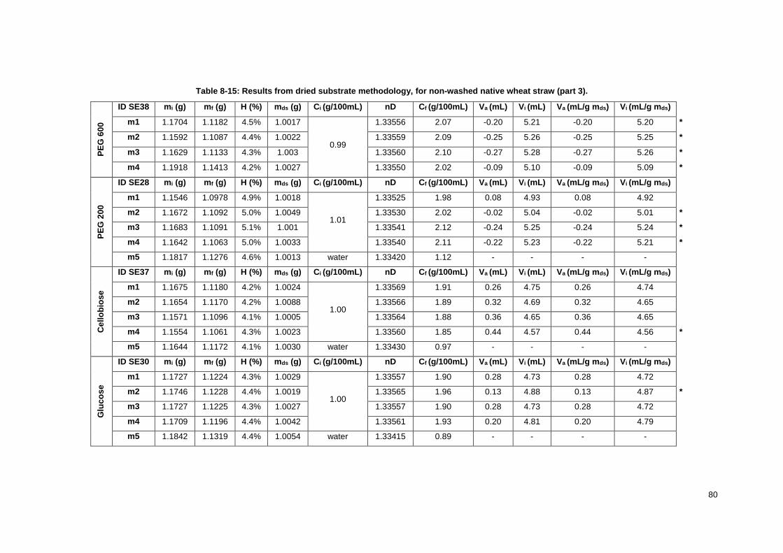
80

Table 8-15: Results from dried substrate methodology, for non-washed native wheat straw (part 3). P

EG

60

0


m1 1.1704 1.1182 4.5% 1.0017

0.99

1.33556 2.07 -0.20 5.21 -0.20 5.20 *

m2 1.1592 1.1087 4.4% 1.0022 1.33559 2.09 -0.25 5.26 -0.25 5.25 *

m3 1.1629 1.1133 4.3% 1.003 1.33560 2.10 -0.27 5.28 -0.27 5.26 *

m4 1.1918 1.1413 4.2% 1.0027 1.33550 2.02 -0.09 5.10 -0.09 5.09 *

PE

G 2

00


m1 1.1546 1.0978 4.9% 1.0018

1.01

1.33525 1.98 0.08 4.93 0.08 4.92

m2 1.1672 1.1092 5.0% 1.0049 1.33530 2.02 -0.02 5.04 -0.02 5.01 *

m3 1.1683 1.1091 5.1% 1.001 1.33541 2.12 -0.24 5.25 -0.24 5.24 *

m4 1.1642 1.1063 5.0% 1.0033 1.33540 2.11 -0.22 5.23 -0.22 5.21 *

m5 1.1817 1.1276 4.6% 1.0013 water 1.33420 1.12 - - - -

Cell

ob

iose


m1 1.1675 1.1180 4.2% 1.0024

1.00

1.33569 1.91 0.26 4.75 0.26 4.74

m2 1.1654 1.1170 4.2% 1.0088 1.33566 1.89 0.32 4.69 0.32 4.65

m3 1.1571 1.1096 4.1% 1.0005 1.33564 1.88 0.36 4.65 0.36 4.65

m4 1.1554 1.1061 4.3% 1.0023 1.33560 1.85 0.44 4.57 0.44 4.56 *

m5 1.1644 1.1172 4.1% 1.0030 water 1.33430 0.97 - - - -

Glu

co

se


m1 1.1727 1.1224 4.3% 1.0029

1.00

1.33557 1.90 0.28 4.73 0.28 4.72

m2 1.1746 1.1228 4.4% 1.0019 1.33565 1.96 0.13 4.88 0.13 4.87 *

m3 1.1727 1.1225 4.3% 1.0027 1.33557 1.90 0.28 4.73 0.28 4.72

m4 1.1709 1.1196 4.4% 1.0042 1.33561 1.93 0.20 4.81 0.20 4.79

m5 1.1842 1.1319 4.4% 1.0054 water 1.33415 0.89 - - - -

81

Table 8-16: Results from dried substrate methodology, for non-washed native wheat straw – nD correction (part 1).

PE

G 3

50

00

ID SE31 nD nD’ Cf (g/100mL) Ve (mL) Va (mL) Vi (mL) Ve (mL/g mds) Va (mL/g mds) Vi (mL/g mds)

m1 1.33560 1.33426 1.02 9.85 0 0.15 9.84 0 0.15

m2 1.33556 1.33422 0.99 10.15 0 -0.15 10.11 0 -0.15 *

m3 1.33561 1.33427 1.03 9.78 0 0.22 9.78 0 0.22

m4 1.33565 1.33431 1.06 9.51 0 0.49 9.49 0 0.49 *

PE

G 2

00

00

ID SE21 nD nD’ Cf (g/100mL) Va (mL) Vi (mL) Va (mL/g mds) Vi (mL/g mds)

m1 1.33560 1.33426 1.03 -0.07 0.25 -0.07 0.25 **

m2 1.33559 1.33425 1.02 0.00 0.18 0.00 0.18 **

m3 1.33557 1.33423 1.00 0.15 0.03 0.15 0.03 *

m4 1.33559 1.33425 1.02 0.00 0.18 0.00 0.18 **

PE

G 8

00

0


m1 1.33561 1.33427 1.04 -0.20 0.38 -0.20 0.38 *

m2 1.33554 1.33420 0.99 -0.20 -0.13 -0.20 -0.13 *

m3 1.33558 1.33424 1.02 0.02 0.17 0.02 0.17

m4 1.33558 1.33424 1.02 0.02 0.17 0.02 0.17

PE

G 4

00

0


m1 1.33559 1.33425 1.03 -0.07 0.25 -0.07 0.25 *

m2 1.33557 1.33423 1.01 0.08 0.10 0.08 0.10

m3 1.33556 1.33422 1.00 0.15 0.03 0.15 0.03

m4 1.33569 1.33435 1.10 -0.74 0.92 -0.74 0.92 *

PE

G 2

00

0


m1 1.33551 1.33417 0.90 1.31 -1.13 1.30 -1.12 *

m2 1.33554 1.33420 0.93 1.00 -0.81 0.99 -0.81 *

m3 1.33558 1.33424 0.96 0.60 -0.42 0.60 -0.42 *

m4 1.33559 1.33425 0.97 0.51 -0.33 0.51 -0.33 *

82

Table 8-17: Results from dried substrate methodology, for non-washed native wheat straw – nD correction (part 2).

PE

G 1

50

0


m1 1.33556 1.33422 1.01 0.10 0.08 0.10 0.08

m2 1.33555 1.33421 1.00 0.17 0.01 0.17 0.01

m3 1.33556 1.33422 1.01 0.10 0.08 0.10 0.08

m4 1.33557 1.33423 1.02 0.03 0.16 0.03 0.16 *

PE

G 6

00


m1 1.33556 1.33422 1.05 -0.37 0.55 -0.37 0.55 *

m2 1.33559 1.33425 1.07 -0.57 0.76 -0.57 0.75 *

m3 1.33560 1.33426 1.08 -0.64 0.82 -0.64 0.82 *

m4 1.33550 1.33416 1.00 0.06 0.12 0.06 0.12

PE

G 2

00


m1 1.33525 1.33391 0.88 1.61 -1.42 1.60 -1.42 ***

m2 1.33530 1.33396 0.92 1.09 -0.91 1.09 -0.91 ***

m3 1.33541 1.33407 1.01 0.11 0.07 0.11 0.07 *

m4 1.33540 1.33406 1.00 0.20 -0.01 0.19 -0.01 ***

Cell

ob

iose


m1 1.33569 1.33435 1.00 0.19 -0.01 0.19 -0.01 ***

m2 1.33566 1.33432 0.98 0.40 -0.22 0.40 -0.22 ***

m3 1.33564 1.33430 0.97 0.54 -0.36 0.54 -0.36 ***

m4 1.33560 1.33426 0.94 0.84 -0.66 0.84 -0.66 ***

Glu

co

se


m1 1.33557 1.33423 0.95 0.69 -0.51 0.69 -0.51 ***

m2 1.33565 1.33431 1.01 0.10 0.08 0.10 0.08 *

m3 1.33557 1.33423 0.95 0.69 -0.51 0.69 -0.51 ***

m4 1.33561 1.33427 0.98 0.38 -0.20 0.38 -0.20 ***

83

Dried substrate methodology – Washed native wheat straw

Results that present a significant deviation were not considered in calculations (signed with an asterisk – *). For the molecules with high diameter, when

the result of determination of accessible volume is negative, is considered zero for the treatment of the data (signed with double asterisk – **).

Table 8-18: Results from dried substrate methodology, for washed native wheat straw.

PE

G 3

50

00


m1 1.6907 0.6721 60.2% 0.4999

1.01

1.33436 1.09 4.63 0 0.37 9.25 0 0.75

m2 1.6220 0.6361 60.8% 0.5000 1.33434 1.07 4.69 0 0.31 9.38 0 0.62 *

m3 1.6363 0.6451 60.6% 0.5019 1.33438 1.10 4.56 0 0.44 9.09 0 0.87 *

m4 1.1974 0.4705 60.7% 0.5007 1.33436 1.09 4.63 0 0.37 9.24 0 0.75

m5 - - - 0.4503 water 1.33286 -0.02 - - - -

PE

G 2

00

00


m1 1.2021 0.4764 60.4% 0.4804

1.00

1.33436 1.09 -0.01 0.38 -0.02 0.80 *

m2 1.2086 0.4745 60.7% 0.4828 1.33434 1.07 0.05 0.32 0.11 0.67

m3 1.2223 0.4736 61.3% 0.4825 1.33437 1.09 -0.04 0.41 -0.08 0.86 *

m4 1.2308 0.4957 59.7% 0.5045 1.33433 1.07 0.08 0.29 0.17 0.58

m5 1.1954 0.4913 58.9% 0.4986 water 1.33302 0.12 - - - -

Glu

co

se


m1 1.2972 0.5258 59.5% 0.5011

1.00

1.33451 1.14 -0.23 0.60 -0.46 1.20

m2 1.2914 0.5083 60.6% 0.5020 1.33451 1.14 -0.23 0.60 -0.45 1.20

m3 1.2993 0.5169 60.2% 0.5002 1.33451 1.14 -0.23 0.60 -0.46 1.20

m4 1.2731 0.2311 81.8% 0.2883 1.33451 1.14 -0.23 0.60 -0.79 2.09

m5 1.2987 0.5020 61.3% 0.5013 water 1.33303 0.10 - - - -

84

Table 8-19: Results from dried substrate methodology, for washed native wheat straw – nD correction.

PE

G 3

50

00

ID SE32 nD nD’ Cf (g/100mL) Ve (mL) Va (mL) Vi (mL) Ve (mL/g mds) Va (mL/g mds) Vi (mL/g mds)

m1 1.33449 1.33435 1.08 9.26 0 0.74 9.23 0 0.74

m2 1.33448 1.33434 1.08 9.32 0 0.68 9.27 0 0.68

m3 1.33449 1.33435 1.08 9.26 0 0.74 9.19 0 0.74

m4 1.33451 1.33437 1.10 9.13 0 0.87 9.10 0 0.87 *

PE

G 2

00


m1 1.33426 1.33412 1.05 0.37 0.35 0.37 0.35

m2 1.33424 1.33410 1.03 0.51 0.21 0.51 0.21 *

m3 1.33426 1.33412 1.05 0.37 0.35 0.37 0.35

m4 1.33430 1.33416 1.08 0.10 0.62 0.10 0.62 *

Glu

co

se


m1 1.33446 1.33432 1.01 0.65 0.07 0.65 0.07

m2 1.33447 1.33433 1.02 0.58 0.14 0.58 0.14

m3 1.33447 1.33433 1.02 0.58 0.14 0.58 0.14

m4 1.33450 1.33436 1.04 0.38 0.34 0.38 0.34 *

85

Dried substrate methodology – Wheat straw pretreated at 160 °C and washed

Results that present a significant deviation were not considered in calculations (signed with an asterisk – *). For the molecules with high diameter, when

the result of determination of accessible volume is negative, is considered zero for the treatment of the data (signed with double asterisk – **).

Table 8-20: Results from dried substrate methodology, for wheat straw pretreated at 160 °C and washed.

PE

G 3

50

00


m1 6.4620 1.2814 80.2% 1.0023

1.00

1.33449 1.19 8.47 0 1.53 8.45 0 1.53

m2 6.7528 1.3003 80.7% 1.0053 1.33448 1.18 8.52 0 1.48 8.47 0 1.47

m3 6.0815 1.1687 80.8% 1.0068 1.33449 1.19 8.47 0 1.53 8.41 0 1.52

m4 6.2017 1.2963 79.1% 1.0030 1.33451 1.20 8.36 0 1.64 8.34 0 1.63 *

m5 6.1016 1.3021 78.7% 1.0078 water 1.33301 0.09 - - - - -

PE

G 2

00


m1 6.2351 1.3581 78.2% 1.0016

1.01

1.33426 1.15 0.30 1.22 0.30 1.22

m2 6.0296 1.2350 79.5% 1.0014 1.33424 1.14 0.41 1.10 0.41 1.10 *

m3 6.1902 1.2227 80.2% 1.0094 1.33426 1.15 0.30 1.22 0.29 1.21

m4 6.2415 1.1663 81.3% 1.0017 1.33430 1.18 0.07 1.45 0.07 1.44 *

m5 6.0455 1.2929 78.6% 1.0002 water 1.33301 0.20 - - - -

Glu

co

se


m1 6.0339 1.1702 80.6% 1.0042

1.00

1.33446 1.10 0.59 0.93 0.59 0.92

m2 6.0001 1.1951 80.1% 1.0012 1.33447 1.11 0.53 0.98 0.53 0.98

m3 6.0204 1.1364 81.1% 1.0014 1.33447 1.11 0.53 0.98 0.53 0.98

m4 6.0270 1.1631 80.7% 1.0002 1.33450 1.13 0.37 1.15 0.37 1.15 *

m5 6.0273 1.2072 80.0% 1.0006 water 1.33297 0.07 - - - -

86

Pore volume distributions for dried substrate methodology

To the standard deviation of the results, a 98% of confidence interval was applied to the data.

Results that present a significant deviation were not considered in calculations (signed with an

asterisk – *). For the molecules with high diameter, when the result of determination of accessible

volume is negative, is considered zero for the treatment of the data (signed with double asterisk – **).

Table 8-21: Pore volume distribution data for Alphacel.

Probe Diameter (Ǻ) Ve (mL/g mds) Va (mL/g mds) Vi (mL/g mds)

PEG 20000 130 9.17±0.03 0 0.77±0.04

PEG 10000 90 9.17±0.03 0 0.77±0.04

PEG 8000 84 9.17±0.03 0.04±0.00 0.73±0.00

PEG 2000 40 9.17±0.03 0.08±0.04 0.69±0.03

PEG 1500 33 9.17±0.03 0.10±0.00 0.67±0.00

PEG 600 21 9.17±0.03 0.21±0.03 0.56±0.03

PEG 200 13 9.17±0.03 0.42±0.04 0.37±0.03

Cellobiose 10 9.17±0.03 0.44±0.04 0.33±0.04

Glucose 8 9.17±0.03 0.70±0.00 0.07±0.00

Table 8-22: Pore volume distribution data for non-washed native wheat straw.


PEG 35000 170 4.99±0.01 0 5.01±0.02

PEG 20000 130 4.99±0.01 0 5.01±0.02

Dextran 75000 120 4.99±0.01 0.17±0.00 4.83±0.00 *

PEG 8000 84 4.99±0.01 -0.06±0.03 5.03±0.04 *

PEG 4000 56 4.99±0.01 -0.10±0.10 5.10±0.11 *

PEG 2000 40 4.99±0.01 -0.22±0.07 5.21±0.07 *

PEG 1500 33 4.99±0.01 -0.03±0.01 5.03±0.01 *

PEG 600 21 4.99±0.01 -0.20±0.08 5.20±0.08 *

PEG 200 13 4.99±0.01 0.08±0.00 4.92±0.00

Cellobiose 10 4.99±0.01 0.31±0.05 4.68±0.05

Glucose 8 4.99±0.01 0.26±0.04 4.74±0.04

87

Table 8-23: Pore volume distribution data for non-washed native wheat straw – nD correction.


PEG 35000 170 9.81±0.04 0 0.18±0.05

PEG 20000 130 9.81±0.04 0 0.18±0.05

Dextran 75000 120 9.81±0.04 0.14±0.00 0.04±0.00 *

PEG 8000 84 9.81±0.04 0.02±0.00 0.17±0.00

PEG 4000 56 9.81±0.04 0.11±0.05 0.07±0.15

PEG 2000 40 9.81±0.04 0.85±0.36 -0.67±0.36 *

PEG 1500 33 9.81±0.04 0.12±0.04 0.06±0.04

PEG 600 21 9.81±0.04 0.06±0.00 0.12±0.00

PEG 200 13 9.81±0.04 0.18±0.05 0 **

Cellobiose 10 9.81±0.04 0.18±0.05 0 **

Glucose 8 9.81±0.04 0.18±0.05 0 **

Table 8-24: Pore volume distribution data for washed native wheat straw.


PEG 35000 170 8.44±0.03 0 1.51±0.03

PEG 200 13 8.44±0.03 0.29±0.00 1.21±0.01

Glucose 8 8.44±0.03 0.55±0.03 0.96±0.03

Table 8-25: Pore volume distribution data for washed native wheat straw – nD correction.


PEG 35000 170 9.23±0.04 0 0.72±0.04

PEG 200 13 9.23±0.04 0.37±0.00 0.35±0.00

Glucose 8 9.23±0.04 0.60±0.03 0.12±0.04

Table 8-26: Pore volume distribution data for washed and pretreated wheat straw.


PEG 35000 170 9.25±0.01 0 0.75±0.00

PEG 20000 130 9.25±0.01 0.29±0.00 0.62±0.06

Glucose 8 9.25±0.01 -0.54±0.17 1.42±0.44 *

ethanol 2g: development of a methodology to evaluate the ... · ethanol 2g: development of a...

Documents