etna volume 35, pp. 17-39, 2009. copyright …. l. cardoso †, c. m. fernandes , and r....
TRANSCRIPT

Electronic Transactions on Numerical Analysis.Volume 35, pp. 17-39, 2009.Copyright 2009, Kent State University.ISSN 1068-9613.
ETNAKent State University
http://etna.math.kent.edu
STRUCTURAL AND RECURRENCE RELATIONS FORHYPERGEOMETRIC-TYPE FUNCTIONS BY NIKIFOROV-UVAROV METHO D∗
J. L. CARDOSO†, C. M. FERNANDES†, AND R. ALVAREZ-NODARSE‡
Abstract. The functions of hypergeometric-type are the solutionsy = yν(z) of the differential equationσ(z)y′′ + τ(z)y′ + λy = 0, whereσ andτ are polynomials of degrees not higher than2 and1, respectively,andλ is a constant. Here we consider a class of functions of hypergeometric type: those that satisfy the conditionλ+ ντ ′ + 1
2ν(ν − 1)σ′′ = 0, whereν is an arbitrary complex (fixed) number. We also assume that the coefficients
of the polynomialsσ andτ do not depend onν. To this class of functions belong Gauss, Kummer, and Hermitefunctions, and also the classical orthogonal polynomials.In this work, using the constructive approach introducedby Nikiforov and Uvarov, several structural properties of the hypergeometric-type functionsy = yν(z) are obtained.Applications to hypergeometric functions and classical orthogonal polynomials are also given.
Key words. hypergeometric-type functions, recurrence relations, classical orthogonal polynomials
AMS subject classifications.33C45, 33C05, 33C15
1. Introduction. When solving numerous theoretical and applied quantum mechanicalproblems, one is led to potentials that can be solved analytically; see, e.g., [3, 13, 19, 21, 22,23]. In most cases the Schrodinger equation for such potentials can be transformed into thegeneralized hypergeometric-typedifferential equation [15] which has the form
u′′(z) +τ (z)
σ(z)u′(z) +
σ(z)
σ2(z)u(z) = 0,
whereσ, σ and τ are polynomials,deg[σ] ≤ 2, deg[σ] ≤ 2 anddeg[τ ] ≤ 1. By a certainchange of dependent variable (see [15, Section 1, pp. 1–3]) this equation can be transformedinto the hypergeometric-type equation
(1.1) σ(z)y′′(z) + τ(z)y′(z) + λy(z) = 0 ,
whereσ andτ are polynomials of degrees not higher than two and one, respectively, andλ is aconstant. Their solutions are known ashypergeometric-type functionsand to this class belongthe Bessel, Airy, Weber, Whittaker, Gauss, Kummer, and Hermite functions, the classicalorthogonal polynomials, among others.
The class of functionsy = yν(z) we are dealing with in this work corresponds to thesolutions of the hypergeometric equation (1.1) under the condition
λ + ντ ′ +ν(ν − 1)
2σ′′ = 0,
whereν is a complex number. One basic important property of this class of functions is thattheir derivatives are again hypergeometric-type functions. The converse is also true whendeg[σ(s)] = 2 ∨ deg[τ(s)] = 1: any hypergeometric-type function is the derivative of ahypergeometric-type function. More precisely, we have the following results [15, Section 2,p. 6].
∗Received July 24, 2007. Accepted for publication December 12, 2008. Published online on March 6, 2009.Recommended by F. Marcellan.
†Departamento de Matematica, Universidade de Tras-os-Montes e Alto Douro, Apartado 202, 5001 - 911 VilaReal, Portugal ([email protected],[email protected]).
‡Departamento de Analisis Matematico, Facultad de Matem´atica, Universidad de Sevilla, Apdo. Postal 1160,Sevilla, E-41080, Sevilla, Spain ([email protected]).
17

ETNAKent State University
http://etna.math.kent.edu
18 J. CARDOSA, C. FERNANDES, AND R.ALVAREZ-NODARSE
1. if y = y(z) is a solution of (1.1) then, then-th derivative ofy(z), vn(z) := y(n)(z),is a solution of
(1.2) σ(z)v′′n(z) + τn(z)v′n(z) + µnvn(z) = 0,
where
(1.3) τn(z) = τ(z) + nσ′(z)
and
µn = µn(λ) = λ + nτ ′ +n(n − 1)
2σ′′ ;
2. if vn(z) is a solution of (1.2) andµk 6= 0 for k = 1, . . . , n − 1, thenvn = y(n)(z)wherey = y(z) is a solution of (1.1).
Joining these two properties it is possible to derive many other properties [15, pp. 14, 207,and 265]. Numerous structural properties of this class of functions have been studied in thelast two decades [5, 6, 7, 8, 9, 25, 26].
The recurrence relations for the special functions (and thus for the associated wave func-tions) are interesting not only from the theoretical point of view (they are useful for comput-ing the values of matrix elements of certain physical quantities; see, e.g., [5] and referencestherein), but also they can be used to numerically compute the values of the functions as wellas their derivatives, as is shown in our previous paper [2] for the case of Laguerre polynomi-als and the associated wave functions of the harmonic oscillator and of the hydrogen atom.Nevertheless, we need to point out that, although the recurrence relations seem to be moreuseful for the evaluation of the corresponding functions than other direct methods, one shouldbe very careful when using them; see, e.g., the nice surveys [11, 24] on numerical evaluationand the convergence problem that appears when dealing with recurrence relations, or the mostrecent results [17, 18] for the case of the hypergeometric function2F1.
In the present paper we obtain, in a unified way, several algebraic characteristics (re-currence and structural relations) for the solutions of thehypergeometric equation (1.1), i.e.,for the hypergeometric-type functions. In particular, we find several new recurrence andstructural relations for the solutions of the hypergeometric equation (1.1) in terms of thepolynomial coefficientsσ andτ , namely, Theorems3.3 and3.5; Corollaries3.8, 3.9, 3.10,3.12, and3.14. For the particular cases ofhypergeometric, confluent hypergeometric, andHermiteequations, some of these results can be obtained also by using the properties of thehypergeometric functions; see [16, Section 33]. However, here we will use an alternative andmore generaldirect approach based on the Nikiforov and Uvarov method [15, §3–§4], whichallows us to obtain recurrences relationsa la carte. In this case we concentrate our effort onthe not so well known fourth-term recurrence relations for the hypergeometric-type functions.Another advantage of this method is that it enables derivation of the recurrences in terms ofthe coefficients of the differential equation (1.1), and therefore it can be easily implementedin any computer algebra system; see, e.g., [12].
Finally, let us mention that many of the recurrence relations involving derivatives canbe obtained by appropriate combinations of three recurrence relations of the hypergeometric-type functions; namely, the three-term recurrence relation and the two differentiation formu-las of these functions given in [7]; see identities (5), (27), and (30), pp. 713, 716, and 717,respectively. This technique in not recommended, since thecorresponding computations arecumbersome and the resulting coefficients are not, in general, as simple as the ones we presenthere. Let us also mention that for the case when the coefficientsσ andτ of the equation (1.1)

ETNAKent State University
http://etna.math.kent.edu
RECURRENCE RELATIONS FOR HYPERGEOMETRIC-TYPE FUNCTIONS 19
change with the spectral parameterλ, a general theory that extents the Nikiforov-Uvarov oneis presented in [27].
The structure of the paper is as follows: In Section2 the preliminary results are presented.The main results of the paper are in Section3, where three four-term recurrence relationsare obtained and from them, several three-term recurrence relations are explicitly writtendown. Finally, in Section4, applications to the hypergeometric, confluent hypergeometric,and Hermite functions, as well as to the classical orthogonal polynomials are given.
2. Preliminaries. Here we will follow the notation and results of [15]. The above prop-erties1 and2 allow us to construct a family of particular solutions of (1.1) for a givenλ. Infact, whenµn = 0, (1.2) has the particular solutionvn(z) = C, (constant). By property2,vn(z) = y(n) wherey = y(z) is a solution of (1.1). This means that when
(2.1) λ = λn := −nτ ′ −n(n − 1)
2σ′′,
the equation (1.1) has a (particular) polynomial solutiony(z) = yn(z), with deg[yn(z)] = n.Such polynomials are known aspolynomials of hypergeometric typeand correspond to thecase whenλ = λn is given by (2.1). In particular, for them we have theRodrigues formula
(2.2) yn(z) =Bn
ρ(z)
[
σn(z)ρ(z)](n)
,
where theBn, n = 0, 1, 2, . . ., are normalizing constants andρ(z) is a solution of the Pearsonequation
(2.3)[
σ(z)ρ(z)]′
= τ(z)ρ(z) .
Assuming thatρ is an analytic function on and inside a closed contourC surrounding thepoints = z and making use of the Cauchy’s integral theorem (see, e.g., [10]), we may write
(2.4) yn(z) =Cn
ρ(z)
∫
C
σn(s)ρ(s)
(s − z)(n+1)ds ,
where theCn = n!Bn/(2πi) is a normalizing constant andρ(z) satisfies (2.3). This suggeststo look for a particular solution of (1.1) of the form
(2.5) yν(z) =Cν
ρ(z)
∫
C
σν(s)ρ(s)
(s − z)(ν+1)ds ,
whereCν is a normalizing constant andν is an arbitrary complex parameter connected withλ by
(2.6) λ = λν = −ντ ′ −ν(ν − 1)
2σ′′ .
The following theorem asserts that the above suggestion is true.
Theorem A [15, p. 10]. Let ρ(z) satisfy the Pearson equation (2.3), whereν is a solutionof (2.6), and letD be a region of the complex plane which contains the piecewisesmoothcurveC of finite length. Then, equation (1.1) has a particular solution of the form (2.5)provided that the functionsσ
ν(s)ρ(s)(s−z)(ν+k) , for k = 1, 2,
• are continuous as functions of the variabless ∈ C, z ∈ D ;

ETNAKent State University
http://etna.math.kent.edu
20 J. CARDOSA, C. FERNANDES, AND R.ALVAREZ-NODARSE
• for each fixeds ∈ C, they are analytic as functions ofz ∈ D;
andC is such thatσν+1(s)ρ(s)(s−z)ν+2
∣
∣
∣
s2
s1
= 0, wheres1 ands2 are the endpoints ofC.
If the integral in (2.5) is an improper one, then the result remains valid if the convergence ofthe integral is uniform [10, p. 188].
In the next sections, generalizing (1.3), we will use the notation
(2.7) τν(z) = τ(z) + νσ′(z) = τ ′
ν z + τν(0), ν ∈ C,
and, in order to keep valid property2 of Section1, we will restrict ourselves to the conditiondeg[σ(s)] = 2 ∨ deg[τ(s)] = 1.
3. Recurrence relations for the hypergeometric-type functions. Now we are readyto establish the main results of this paper.
3.1. Four-term recurrence relations. First, we prove the following theorem.THEOREM3.1.Consider the hypergeometric-type functionsy
(k)ν−1(z), y(k)
ν (z), y(k+1)ν (z),
andy(k+1)ν+1 (z) defined by (2.5). Suppose thatρ(z) is a solution of (2.3) and
(3.1)σν(s)ρ(s)
(s − z)ν−k−1sm
∣
∣
∣
∣
∣
s2
s1
= 0, m = 0, 1, 2, ...,
wheres1 and s2 are the end points ofC. Then, there exist polynomial coefficientsAik(z),i = 1, 2, 3, 4, not all identically zero, such that
(3.2) A1k(z)y(k)ν−1(z) + A2k(z)y(k)
ν (z) + A3k(z)y(k+1)ν (z) + A4k(z)y
(k+1)ν+1 (z) = 0.
Moreover, the functionsAik, i = 1, 2, 3, 4 are given by
8
>
>
>
>
>
>
>
>
>
>
>
>
>
>
>
>
>
<
>
>
>
>
>
>
>
>
>
>
>
>
>
>
>
>
>
:
A1k(z) = −τ′ντ
′ν+k−1
2τ′ν+k−2
2
h
τ2ν−1(0)
σ′′
2− τ
′ν−1
“
τν−1(0)σ′(0) − τ
′ν−1σ(0)
”i
×
Cν
Cν−1
“
R(z) − 2σ′(z)
”
,
A2k(z)=(ν−k)τ ′ν2−1τ
′ντ
′ν+k−1
2
»
“
R(z)−2σ′(z)
”
„
τν−1(z)σ′′
2−σ
′(z)τ ′ν−1
«
−τ′ν−1σ
′′σ(z)
–
,
A3k(z)=
"
τ′ντ
′ν+k−1
2R(z) + (ν − k)
(σ′′)2
2τν(z) − 2τ
′
ν− 12τ′νσ
′(z)
#
τ′ν2−1τ
′ν−1σ(z),
A4k(z)=(ν − k)Cν
Cν+1τ′ν2−1τ
′ν−12
τ′ν−1σ
′′σ(z),
(3.3)
whereR(z) is an arbitrary function ofz.Proof. From [15, Eq. (9), p. 17], we have
(3.4) y(k)ν (z) =
C(k)ν
σk(z)ρ(z)
∫
C
σν(s)ρ(s)
(s − z)ν−k+1ds, C(n)
ν =
n−1∏
j=0
τ ′ν+j−1
2
Cν .
Now, using [15, Eqs. (4), p. 16 and (9), p. 17],
(3.5) y(k)ν (z) =
C(k)ν
σk(z)ρ(z)
1
ν − k
∫
C
τν−1(s)σν−1(s)ρ(s)
(s − z)ν−kds.

ETNAKent State University
http://etna.math.kent.edu
RECURRENCE RELATIONS FOR HYPERGEOMETRIC-TYPE FUNCTIONS 21
Substituting the above expressions (3.4) and (3.5) in
S(z) = A1k(z)y(k)ν−1(z) + A2k(z)y(k)
ν (z) + A3k(z)y(k+1)ν (z) + A4k(z)y
(k+1)ν+1 (z),
we obtain
(3.6) S(z) =1
σk+1(z)ρ(z)
∫
C
σν−1(s)ρ(s)
(s − z)ν−kP (s)ds ,
where
P (s) = A1k(z)C(k)ν−1σ(z) + A2k(z)
C(k)ν
ν − kσ(z)τν−1(s) + A3k(z)C(k+1)
ν σ(s) +
A4k(z)C
(k+1)ν+1
ν − kτν(s)σ(s) .(3.7)
Let us define a functionQ(z, s) which is, for every fixedz, a polynomial ins such that
σν−1(s)ρ(s)
(s − z)ν−kP (s) =
∂
∂s
[
σν(s)ρ(s)
(s − z)ν−k−1Q(z, s)
]
.
If such a functionQ exists, then the integral (3.6) vanishs by the boundary conditions (3.1),and therefore (3.2) holds. Let us show that the aforementioned functionQ always exists.
Taking the derivative of the right hand side of the last equality, one gets
(3.8) P (s) = [τν−1(s)(s − z) − (ν − k − 1)σ(s)] Q(z, s) + σ(s)(s − z)∂Q
∂s(z, s) .
Comparing the expressions (3.7) and (3.8), we may conclude that, with respect to the vari-ables, deg [Q(z, s)] = degs [Q(z, s)] ≤ 1. Thus, using the expansions
Q(z, s) = Q(z, z) +∂Q
∂s(z, z)(s − z),
(3.9) τν(s) = τν(z) + τ ′
ν(s − z), σ(s) = σ(z) + σ′(z)(s − z) +σ′′
2(s − z)2 ,
as well as (2.7), we have
8
>
>
>
>
>
>
>
>
>
>
>
>
>
>
>
>
>
>
>
>
>
>
>
>
>
>
>
>
<
>
>
>
>
>
>
>
>
>
>
>
>
>
>
>
>
>
>
>
>
>
>
>
>
>
>
>
>
:
A1k(z)C(k)ν−1σ(z) + A2k(z)
C(k)ν
ν − kτν−1(z)σ(z) + A3k(z)C(k+1)
ν σ(z)+
+A4k(z)C
(k+1)ν+1
ν − kτν(z)σ(z) = −(ν − k − 1)σ(z)Q(z, z),
A2k(z)C
(k)ν
ν − kτ′ν−1σ(z) + A3k(z)C(k+1)
ν σ′(z) + A4k(z)
C(k+1)ν+1
ν − k
ˆ
τν(z)σ′(z)+τ′νσ(z)
˜
=
τk(z)Q(z, z) − (ν − k − 2)σ(z)∂Q
∂s(z, z),
A3k(z)C(k+1)ν
σ′′
2+ A4k(z)
C(k+1)ν+1
ν − k
»
τν(z)σ′′
2+ τ
′νσ
′(z)
–
= τ′ν+k−1
2Q(z, z)+
τk+1(z)∂Q
∂s(z, z),
A4k(z)C
(k+1)ν+1
ν − kτ′νσ
′′ = 2τ′ν+k2
∂Q
∂s(z, z) .
(3.10)
ETNAKent State University
http://etna.math.kent.edu
22 J. CARDOSA, C. FERNANDES, AND R.ALVAREZ-NODARSE
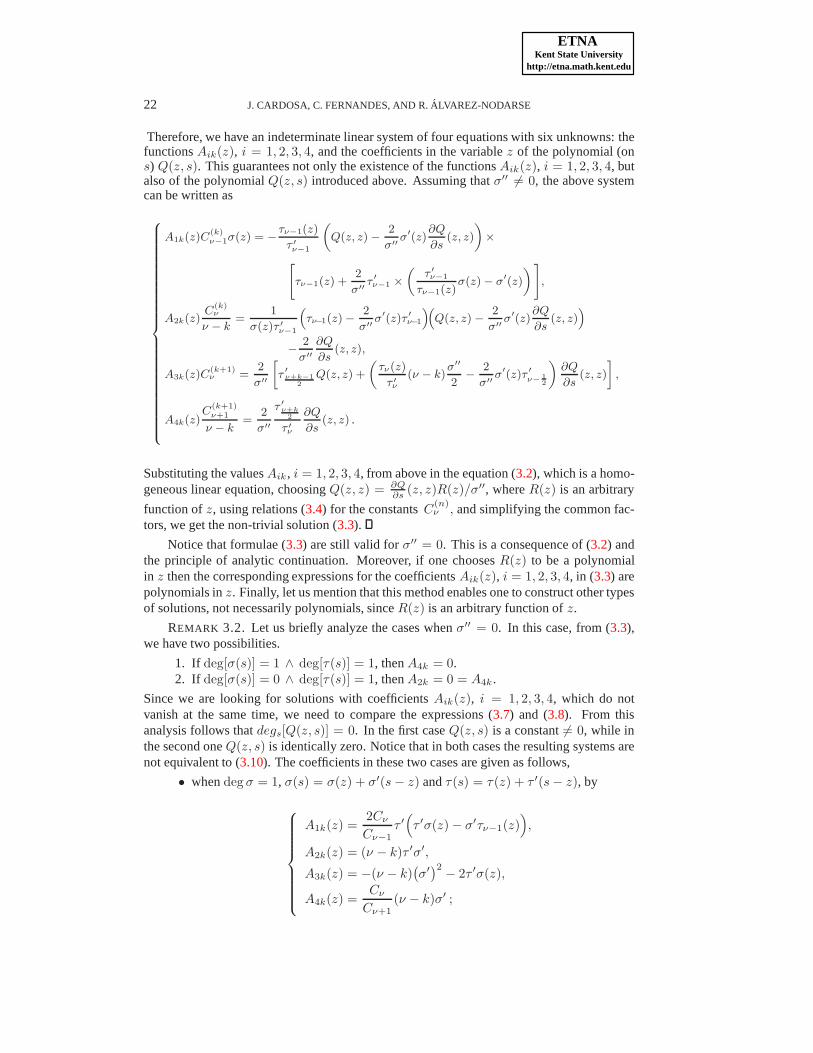
Therefore, we have an indeterminate linear system of four equations with six unknowns: thefunctionsAik(z), i = 1, 2, 3, 4, and the coefficients in the variablez of the polynomial (ons) Q(z, s). This guarantees not only the existence of the functionsAik(z), i = 1, 2, 3, 4, butalso of the polynomialQ(z, s) introduced above. Assuming thatσ′′ 6= 0, the above systemcan be written as
8
>
>
>
>
>
>
>
>
>
>
>
>
>
>
>
>
>
>
>
>
>
>
>
>
>
<
>
>
>
>
>
>
>
>
>
>
>
>
>
>
>
>
>
>
>
>
>
>
>
>
>
:
A1k(z)C(k)ν−1σ(z) = −
τν−1(z)
τ ′ν−1
„
Q(z, z) −2
σ′′σ′(z)
∂Q
∂s(z, z)
«
×
"
τν−1(z) +2
σ′′τ′ν−1 ×
„
τ ′ν−1
τν−1(z)σ(z) − σ
′(z)
«
#
,
A2k(z)C
(k)ν
ν − k=
1
σ(z)τ ′ν−1
“
τν−1(z) −2
σ′′σ′(z)τ ′
ν−1
”“
Q(z, z) −2
σ′′σ′(z)
∂Q
∂s(z, z)
”
−
2
σ′′
∂Q
∂s(z, z),
A3k(z)C(k+1)ν =
2
σ′′
»
τ′ν+k−1
2Q(z, z) +
„
τν(z)
τ ′ν
(ν − k)σ′′
2−
2
σ′′σ′(z)τ ′
ν− 12
«
∂Q
∂s(z, z)
–
,
A4k(z)C
(k+1)ν+1
ν − k=
2
σ′′
τ ′ν+k2
τ ′ν
∂Q
∂s(z, z) .
Substituting the valuesAik, i = 1, 2, 3, 4, from above in the equation (3.2), which is a homo-geneous linear equation, choosingQ(z, z) = ∂Q
∂s(z, z)R(z)/σ′′, whereR(z) is an arbitrary
function ofz, using relations (3.4) for the constantsC(n)ν , and simplifying the common fac-
tors, we get the non-trivial solution (3.3).
Notice that formulae (3.3) are still valid forσ′′ = 0. This is a consequence of (3.2) andthe principle of analytic continuation. Moreover, if one choosesR(z) to be a polynomialin z then the corresponding expressions for the coefficientsAik(z), i = 1, 2, 3, 4, in (3.3) arepolynomials inz. Finally, let us mention that this method enables one to construct other typesof solutions, not necessarily polynomials, sinceR(z) is an arbitrary function ofz.
REMARK 3.2. Let us briefly analyze the cases whenσ′′ = 0. In this case, from (3.3),we have two possibilities.
1. If deg[σ(s)] = 1 ∧ deg[τ(s)] = 1, thenA4k = 0.2. If deg[σ(s)] = 0 ∧ deg[τ(s)] = 1, thenA2k = 0 = A4k.
Since we are looking for solutions with coefficientsAik(z), i = 1, 2, 3, 4, which do notvanish at the same time, we need to compare the expressions (3.7) and (3.8). From thisanalysis follows thatdegs[Q(z, s)] = 0. In the first caseQ(z, s) is a constant6= 0, while inthe second oneQ(z, s) is identically zero. Notice that in both cases the resultingsystems arenot equivalent to (3.10). The coefficients in these two cases are given as follows,
• whendeg σ = 1, σ(s) = σ(z) + σ′(s − z) andτ(s) = τ(z) + τ ′(s − z), by
A1k(z) =2Cν
Cν−1τ ′
(
τ ′σ(z) − σ′τν−1(z))
,
A2k(z) = (ν − k)τ ′σ′,
A3k(z) = −(ν − k)(
σ′)2
− 2τ ′σ(z),
A4k(z) =Cν
Cν+1(ν − k)σ′ ;

ETNAKent State University
http://etna.math.kent.edu
RECURRENCE RELATIONS FOR HYPERGEOMETRIC-TYPE FUNCTIONS 23
• whendeg σ = 0, σ(s) = σ(z) andτ(s) = τ(z) + τ ′(s − z), by
A1k(z) = −Cν
Cν−1τ ′A3k(z),
A2k(z) = −Cν+1
Cν
τ ′A4k(z),
whereA3k(z) andA4k(z) are arbitrary polynomials inz.In a similar fashion we can prove the following theorem.THEOREM 3.3. Consider the functions of hypergeometric typey
(k+1)ν−1 (z), y
(k)ν (z),
y(k+1)ν (z), andy
(k+1)ν+1 (z). Suppose thatρ(z) is a solution of (2.3), satisfying condition (3.1).
Then, there exist polynomial coefficientsBik(z), i = 1, 2, 3, 4, not all identically zero, suchthat
(3.11) B1k(z)y(k+1)ν−1 (z) + B2k(z)y(k)
ν (z) + B3k(z)y(k+1)ν (z) + B4k(z)y
(k+1)ν+1 (z) = 0 .
Moreover, the functionsBik, i = 1, 2, 3, 4, are given by
B1k(z) =Cν
Cν−1τ ′
ντ ′ν+k−1
2
[
τ2ν−1(0)
σ′′
2− τ ′
ν−1
(
τν−1(0)σ′(0) − τ ′
ν−1σ(0))]
×
(
R(z) − 2σ′(z))
,
B2k(z) = −(ν − k)τ ′
ντ ′ν2 −1τ
′ν+k−1
2
[
R(z)τ ′
ν−1 +(
τν−1(z)σ′′ − 2σ′(z)τ ′
ν−1
)]
,
B3k(z)=τ ′
ντ ′ν2−1
[
τ ′ν+k−1
2
R(z) + (ν − k)(σ′′)2
2τ ′ν
τν(z) − 2τ ′
ν− 12σ′(z)
]
τν−1(z),
B4k(z)=(ν − k)σ′′Cν
Cν+1τ ′
ν2−1τ
′ν−12
τν−1(z),
(3.12)
whereR(z) is an arbitrary function ofz.REMARK 3.4. As in Remark3.2, whenσ′′ = 0 from (3.12), the following two cases
apply.1. If deg[σ(s)] = 1 ∧ deg[τ(s)] = 1, thenB4k = 0.2. If deg[σ(s)] = 0 ∧ deg[τ(s)] = 1, thenB4k = 0.
Solving the corresponding systems, we find• deg σ = 1 anddeg τ = 1, σ(s) = σ(z) + σ′(s − z) andτ(s) = τ(z) + τ ′(s − z)
B1k(z) =2Cν
Cν−1
(
σ′τν−1(z) − τ ′σ(z))
,
B2k(z) = (ν − k)τ ′,
B3k(z) = −2τ 3ν−k−22
,
B4k(z) =Cν
Cν+1(ν − k) ;
• deg σ = 0 anddeg τ = 1, σ(s) = σ(z) andτ(s) = τ(z) + τ ′(s − z)
B3k(z) =Cν−1
τ ′Cν
τ(z)A1k(z),
B4k(z) = −Cν−1
τ ′Cν+1(ν − k)A1k(z) −
Cν
τ ′Cν+1A2k(z) ,
whereB1k(z) andB2k(z) are arbitrary polynomials inz.
ETNAKent State University
http://etna.math.kent.edu
24 J. CARDOSA, C. FERNANDES, AND R.ALVAREZ-NODARSE
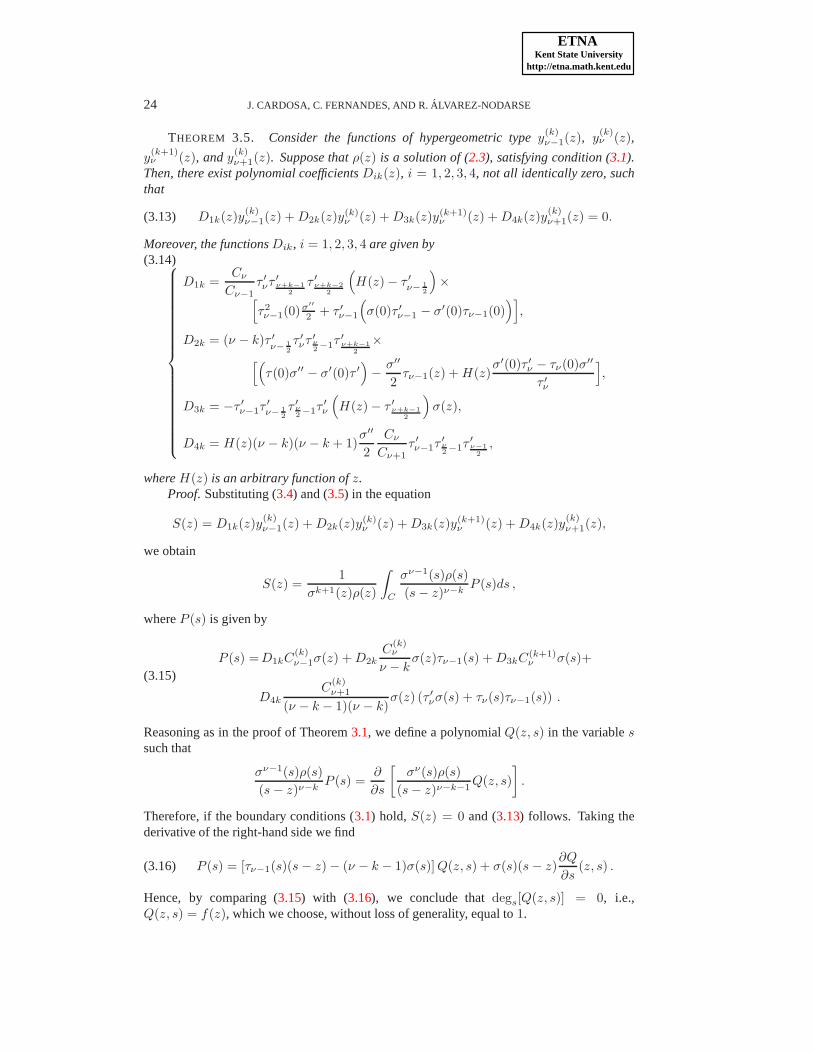
THEOREM 3.5. Consider the functions of hypergeometric typey(k)ν−1(z), y
(k)ν (z),
y(k+1)ν (z), andy
(k)ν+1(z). Suppose thatρ(z) is a solution of (2.3), satisfying condition (3.1).
Then, there exist polynomial coefficientsDik(z), i = 1, 2, 3, 4, not all identically zero, suchthat
(3.13) D1k(z)y(k)ν−1(z) + D2k(z)y(k)
ν (z) + D3k(z)y(k+1)ν (z) + D4k(z)y
(k)ν+1(z) = 0.
Moreover, the functionsDik, i = 1, 2, 3, 4 are given by(3.14)
D1k =Cν
Cν−1τ ′
ντ ′ν+k−1
2
τ ′ν+k−2
2
(
H(z) − τ ′
ν− 12
)
×[
τ2ν−1(0)σ′′
2 + τ ′ν−1
(
σ(0)τ ′ν−1 − σ′(0)τν−1(0)
)]
,
D2k = (ν − k)τ ′
ν− 12
τ ′ντ ′
ν2−1τ
′ν+k−1
2
×
[(
τ(0)σ′′ − σ′(0)τ ′
)
−σ′′
2τν−1(z) + H(z)
σ′(0)τ ′ν − τν(0)σ′′
τ ′ν
]
,
D3k = −τ ′
ν−1τ′
ν− 12τ ′
ν2 −1τ
′
ν
(
H(z) − τ ′ν+k−1
2
)
σ(z),
D4k = H(z)(ν − k)(ν − k + 1)σ′′
2
Cν
Cν+1τ ′
ν−1τ′ν2 −1τ
′ν−12
,
whereH(z) is an arbitrary function ofz.Proof. Substituting (3.4) and (3.5) in the equation
S(z) = D1k(z)y(k)ν−1(z) + D2k(z)y(k)
ν (z) + D3k(z)y(k+1)ν (z) + D4k(z)y
(k)ν+1(z),
we obtain
S(z) =1
σk+1(z)ρ(z)
∫
C
σν−1(s)ρ(s)
(s − z)ν−kP (s)ds ,
whereP (s) is given by
P (s) =D1kC(k)ν−1σ(z) + D2k
C(k)ν
ν − kσ(z)τν−1(s) + D3kC(k+1)
ν σ(s)+
D4k
C(k)ν+1
(ν − k − 1)(ν − k)σ(z) (τ ′
νσ(s) + τν(s)τν−1(s)) .
(3.15)
Reasoning as in the proof of Theorem3.1, we define a polynomialQ(z, s) in the variablessuch that
σν−1(s)ρ(s)
(s − z)ν−kP (s) =
∂
∂s
[
σν(s)ρ(s)
(s − z)ν−k−1Q(z, s)
]
.
Therefore, if the boundary conditions (3.1) hold, S(z) = 0 and (3.13) follows. Taking thederivative of the right-hand side we find
(3.16) P (s) = [τν−1(s)(s − z) − (ν − k − 1)σ(s)] Q(z, s) + σ(s)(s − z)∂Q
∂s(z, s) .
Hence, by comparing (3.15) with (3.16), we conclude thatdegs[Q(z, s)] = 0, i.e.,Q(z, s) = f(z), which we choose, without loss of generality, equal to1.

ETNAKent State University
http://etna.math.kent.edu
RECURRENCE RELATIONS FOR HYPERGEOMETRIC-TYPE FUNCTIONS 25
Substituting the expansions (3.9) of τν−1(s), τν(s), andσ(s) in powers ofs−z in (3.15)and (3.16), we obtain
D1kC(k)ν−1 + D2k
C(k)ν
ν − kτν−1(z) + D3k(z)C(k+1)
ν +
D4k
C(k)ν+1
(ν − k)(ν − k + 1)[τ ′
νσ(z) + τν(z)τν−1(z)] = −(ν − k − 1),
D2k
C(k)ν
ν − kσ(z)τ ′
ν−1+ D3kC(k+1)ν σ′(z) + D4k
C(k)ν+1
(ν − k)(ν − k + 1)σ(z)2τν(z)τ ′
ν− 12
= τk(z),
D3kC(k+1)ν
σ′′
2+ D4k
C(k)ν+1
(ν − k)(ν − k + 1)σ(z)τ ′
ντ ′
ν− 12
= τ ′ν+k−1
2
.
Assumingσ′′ 6= 0, from last equation we get
D3k(z)C(k+1)ν =
2
σ′′
[
τ ′ν+k−1
2
− D4k(z)C
(k)ν+1
(ν − k)(ν − k + 1)σ(z)τ ′
ντ ′
ν− 12
]
.
Choosing now
D4k(z) = R(z)τ ′ν+k−1
2
(ν − k)(ν − k + 1)
C(k)ν+1σ(z)τ ′
ντ ′
ν− 12
,
whereR(z) is an arbitrary function ofz, we obtain
D3k(z)C(k+1)ν =
2
σ′′τ ′
ν+k−12
(1 − R(z)) ,
and therefore8
>
>
>
>
>
>
>
>
>
>
>
>
>
>
>
>
>
>
<
>
>
>
>
>
>
>
>
>
>
>
>
>
>
>
>
>
>
:
D4k(z) = R(z)τ ′ν+k−1
2
(ν − k)(ν − k + 1)
C(k)ν+1τ
′ντ ′
ν− 12
,
D3k(z)C(k+1)ν =
2
σ′′τ′ν+k−1
2
“
1 − R(z)”
σ(z),
D2k(z)C(k)ν =
ν − k
τ ′ν−1
»
2
„
τ (0)−σ′(0)
σ′′τ′
«
−τν−1(z)+2R(z)τ ′ν+k−1
2
„
σ′(0)
σ′′−
τν(0)
τ ′ν
«–
,
D1k(z)C(k)ν−1 =−
τν−1(z)
τ ′ν−1
»
τν−1(z)−2
σ′′τ′ν−1+2R(z)τ ′
ν+k−12
„
σ′(0)
σ′′−
τν(0)
τ ′ν
«–
−
(ν − k − 1)σ(z)−R(z)τ ′ν+k−1
2
τ ′νσ(z)+τν(z)τν−1(z)
τ ′ντ ′
ν− 12
−
2
σ′′σ(z)τ ′
ν+k−12
(1−R(z)).
If we now substitute the above valuesDik, i = 1, 2, 3, 4, in (3.13), putR(z) = H(z)/τ ′ν+k−1
2
,
whereH(z) is a function ofz, and simplify the resulting expressions, we obtain the val-ues (3.14).
Notice that if we chooseH(z) to be a polynomial inz, then the corresponding coeffi-cientsAik, i = 1, 2, 3, 4, will be polynomials inz, too. Formulae (3.14) are still valid, byanalytic continuation, whenσ′′ = 0.
REMARK 3.6. In the case whenσ′′ = 0, from (3.14), the following two cases apply.

ETNAKent State University
http://etna.math.kent.edu
26 J. CARDOSA, C. FERNANDES, AND R.ALVAREZ-NODARSE
1. If deg[σ(s)] = 1 ∧ deg[τ(s)] = 1, thenD4k(z) = 0.2. If deg[σ(s)] = 0 ∧ deg[τ(s)] = 1, thenD2k(z) = 0 = A4k(z).
Thus, a similar analysis yields• in the first case,σ(s) = σ(z) + σ(s − z) andτ(s) = τ(z) + τ ′(s − z)
D1k(z) =2Cν
Cν−1τν(z)
(
τ ′σ(z) − σ′τν−1(z))
,
D2k(z) = (ν − k)σ′τν(z),
D3k(z) = −2τ 3ν−k2
σ(z),
D4k(z) =Cν
Cν+1(ν − k − 1)(ν − k)σ′ ;
• in the second caseσ(s) = σ(z) andτ(s) = τ(z) + τ ′(s − z)
D1k(z) = −Cν
Cν−1(ν − k − 1)τ ′σ(z),
D2k(z) = −(ν − k)τ(z),
D3k(z) = σ(z),
D4k(z) =Cν
Cν+1(ν − k − 1)(ν − k).
3.2. Three-term recurrence relations. In general, in order to obtain three-term recur-rence relations involving functions of hypergeometric type and their derivatives of any order,one could follow the technique described in the previous section; see, e.g., [25]. Here we willobtain several three-term recurrence relations that follow from Theorem3.1(Corollaries3.7–3.9), Theorem3.3 (Corollary 3.10) and Theorem3.5 (Corollaries3.11–3.14), when one ofthe coefficientsAik(z), i = 1, 2, 3, 4, is chosen to be identically zero. Since the proofs of allCorollaries are quite similar we will include here only the first one.
COROLLARY 3.7.
(3.17) E1k(z)y(k)ν (z) + E2k(z)y(k+1)
ν (z) + E3k(z)y(k+1)ν+1 (z) = 0,
E1k(z) = −τ ′ν+k−1
2
τ ′ν ,
E2k(z) = −τ ′νσ′(0) + σ′′
2 (τν(0) − τ ′νz) ,
E3k(z) =Cν
Cν+1τ ′
ν−12
.
(3.18)
Proof. Using the fact thatR(z) in Theorem3.1 is an arbitrary polynomial ofz andputtingR(z) = 2σ′(z), we getA1k = 0. Thus, relation (3.2) becomes
E1k(z)y(k)ν (z) + E2k(z)y(k+1)
ν (z) + E3k(z)y(k+1)ν+1 (z) = 0 ,
where the coefficientsE1k = A2k, E2k = A3k andE3k = A4k are given by
E1k(z) = −(ν − k)τ ′ν+k−1
2
σ′′σ(z),
E2k(z) =ν − k
τ ′ν
σ′′σ(z)
[
−1
2(2τ ′
νσ′(0) + τ ′
νσ′′z − τν(0)σ′′)
]
,
E3k(z) = (ν − k)Cν
Cν+1
τ ′ν−12
τ ′ν
σ′′σ(z).

ETNAKent State University
http://etna.math.kent.edu
RECURRENCE RELATIONS FOR HYPERGEOMETRIC-TYPE FUNCTIONS 27
Hence, after some simplifications, we obtain (3.18).The previous three-term recurrence relation was publishedin [9, relations (6)–(7), p. 663].
COROLLARY 3.8.
(3.19) F1k(z)y(k)ν−1(z) + F2k(z)y(k)
ν (z) + F3k(z)y(k+1)ν+1 (z) = 0,
F1k(z) =Cν
Cν−1τ ′
ν+k−22
[
τν−1(0)
(
τ ′
ν−1σ′(0) −
σ′′
2τν−1(0)
)
−(
τ ′
ν−1
)2σ(0)
]
×
(
σ′′
2τ ′
νz + σ′(0)τ ′
ν −σ′′
2τν(0)
)
,
F2k(z) = (ν − k)τ ′ν2 −1
(
σ′′
2τ ′
νz + σ′(0)τ ′
ν −σ′′
2τν(0)
)
×
(σ′′
2τν−1(0) − σ′(0)τ ′
ν−1 −σ′′
2τ ′
ν−1z)
− τ ′ν2−1τ
′ν+k−1
2
τ ′
ν−1τ′
νσ(z),
F3k(z) =Cν
Cν+1τ ′
ν2−1τ
′ν−12
τ ′
ν−1σ(z).
(3.20)
COROLLARY 3.9.
G1k(z)y(k)ν−1(z) + G2k(z)y(k+1)
ν (z) + G3k(z)y(k+1)ν+1 (z) = 0,
G1k(z) = −Cν
Cν−1τ ′
ν+k−12
τ ′ν+k−2
2
τ ′
ν
[
τ2ν−1(0)σ′′ − 2τ ′
ν−1
(
τν−1(0)σ′(0) − τ ′
ν−1σ(0))]
,
G2k(z) =ν − k
2τ ′
ν2−1
(
τν(0)σ′′− 2σ′(0)τ ′
ν − σ′′τ ′
νz)
×(
τν−1(0)σ′′ − 2σ′(0)τ ′
ν−1 − σ′′τ ′
ν−1z)
+ 2τ ′ν2 −1τ
′ν+k−1
2
τ ′
ν−1τ′
νσ(z),
G3k(z) = (ν − k)Cν
Cν+1τ ′
ν2−1τ
′ν−12
(
τν−1(0)σ′′ − 2σ′(0)τ ′
ν−1 − σ′′τ ′
ν−1z)
.
COROLLARY 3.10.
I1k(z)y(k+1)ν−1 (z) + I2k(z)y(k)
ν (z) + I3k(z)y(k+1)ν+1 (z) = 0,
I1k(z) =Cν
Cν−1
[
τν−1(0)(
σ′(0)τ ′
ν−1 −σ′′
2τν−1(0)
)
−(
τ ′
ν−1
)2σ(0)
]
×[
σ′(0)τ ′ν − σ′′
2
(
τν(0) − τ ′νz)]
,
I2k(z) = (ν − k − 1)τ ′ν2 −1τ
′ν
(
σ′(0)τ ′ν−1 −
σ′′
2 τν−1(0))
+ τν(0)τ ′ν2−1τ
′ν+k2
τ ′ν−1
+τ ′ν2−1τ
′ν−1τ
′
ν− 12
τ ′νz,
I3k(z) = −Cν
Cν+1τ ′
ν2 −1τ
′ν−12
τν−1(z) .

ETNAKent State University
http://etna.math.kent.edu
28 J. CARDOSA, C. FERNANDES, AND R.ALVAREZ-NODARSE
COROLLARY 3.11.
J1k(z)y(k)ν−1(z) + J2k(z)y(k)
ν (z) + J3k(z)y(k)ν+1(z) = 0,
J1k(z) =Cν
Cν−1τ ′
ν+k−22
τ ′
ν
[
τ ′
ν−1
(
σ′(0)τν−1(0) − σ(0)τ ′
ν−1
)
− τ2ν−1(0)
σ′′
2
]
,
J2k(z) = −τ ′ν2−1τ
′
ν− 12
[
τ ′
ντ ′
ν−1z + τ ′τ2ν−k(0) + σ′′(
kτ(0) − τν(1−ν)(0))]
,
J3k(z) = (ν − k + 1)Cν
Cν+1τ ′
ν2−1τ
′ν−12
τ ′
ν−1.
This Corollary was first published in [25, relations (5)–(8), p. 713] and it is nothing else thanthestandardthree-term recurrence relation for the derivative of any order of the hypergeo-metric function.
COROLLARY 3.12.
L1k(z)y(k)ν (z) + L2k(z)y(k+1)
ν (z) + L3k(z)y(k)ν+1(z) = 0,
L1k(z) = τ ′ν+k−1
2
τν(z),
L2k(z) = τ ′
νσ(z),
L3k(z) = −(ν − k + 1)Cν
Cν+1τ ′
ν−12
.
COROLLARY 3.13.
M1k(z)y(k)ν−1(z) + M2k(z)y(k)
ν (z) + M3k(z)y(k+1)ν (z) = 0,
M1k(z) = −Cν
Cν−1τ ′
ν+k−22
[
τ2ν−1(0)
σ′′
2+ τ ′
ν−1
(
σ(0)τ ′
ν−1 − σ′(0)τν−1(0))
]
,
M2k(z) = −ν − k
2τ ′
ν2 −1τ
′
ν−1
(
σ′′z + 2σ′(0) − σ′′τν−1(0)
τ ′ν−1
)
,
M3k(z) = τ ′ν2 −1τ
′
ν−1σ(z).
The above relation was first obtained in [7, relations (30)–(31), p. 717].COROLLARY 3.14.
N1k(z)y(k)ν−1(z) + N2k(z)y(k+1)
ν (z) + N3k(z)y(k)ν+1(z) = 0,
N1k(z) =Cν
Cν−1τ ′
ν+k−22
τ ′ν+k−1
2
×[
τν−1(0)(
2σ′(0)τ ′ν−12
− τ(0)σ′′
)
− 2(
τ ′
ν−1
)2σ(0)
]
τν(z),
N2k(z) = 2τ ′ν2 −1τ
′
ν− 12
[
τ ′
ντ ′
ν−1z + τν(0)τ ′
k−1 + τ ′
νσ′(0)(ν − k)]
σ(z),
N3k(z) = −(ν−k)(ν − k + 1)Cν
Cν+1τ ′
ν2−1τ
′ν−12
[
σ′′τ ′
ν−1z + 2σ′(0)τ ′ν−12
−σ′′τ(0)]
.

ETNAKent State University
http://etna.math.kent.edu
RECURRENCE RELATIONS FOR HYPERGEOMETRIC-TYPE FUNCTIONS 29
REMARK 3.15. To conclude this section let us mention that, in spite of the fact thatthe Nikiforov and Uvarov method used here allows us to obtainthe recurrence relations inTheorems3.1and3.3directly, in principle, Theorem3.1can be obtained also by combiningappropriately the known Corollaries3.7 and3.13. In a similar way, it is possible to obtainTheorem3.3by a suitable combination of Corollaries3.7and3.10. Finally, we point out thatthe Nikiforov and Uvarov technique is required in order to obtain the new Corollary3.10.
4. Applications.
4.1. Recurrence relations for hypergeometric-type functions. We can reduce equa-tion (1.1) to a canonical form by a linear change of independent variable. According to[15, 16], there exist three different cases, corresponding to the different possibilities for thedegree ofσ:
• deg(
σ(z))
= 2 :
(4.1) z(1 − z)u′′ +[
γ −(
α + β + 1)
z]
u′ − αβ u = 0.
This corresponds to equation (1.1) with
(4.2) σ(z) = z(1 − z), τ(z) = γ −(
α + β + 1)
z, λ = −αβ .
• deg(
σ(z))
= 1 :
(4.3) z u′′ +(
γ − z)
u′ − α u = 0 .
This is equation (1.1) with
(4.4) σ(z) = z, τ(z) = γ − z, λ = −α .
• deg(
σ(z))
= 0 :
(4.5) u′′ − 2z u′ + 2ν u = 0 .
This corresponds to equation (1.1) with
(4.6) σ(z) = 1, τ(z) = −2z, λ = 2ν .
Equations (4.1), (4.3), and (4.5) are known as thehypergeometric, confluent hypergeometric,andHermiteequations, respectively. Explicit solutions of these three different equations arewell known; see, e.g., [15, 16]. In [15, §20, Section 2, p. 258] particular solutions were foundusing the corresponding integral representations: the hypergeometricF (α, β, γ, z), confluenthypergeometricF (α, γ, z), and HermiteHν(z) functions. In terms of the generalized hyper-geometric notation [4], the first two correspond to2F1(α, β; γ; z) and1F1(α; γ; z), respec-tively. We will use, for these functions, the normalizationconsidered in [15, §20, Section 2,p. 255].
We remark that ifσ(z) has a double root, then the generalized hypergeometric-typeequa-tion can be reduced to an equation where the correspondingσ(z) is of degree one [15, pp. 3,4].
Here we will present recurrence relations that follow from Theorems3.1, 3.3, and3.5,and some particular examples from the corresponding Corollaries. In the sequel,R(z) repre-sents an arbitrary function ofz.

ETNAKent State University
http://etna.math.kent.edu
30 J. CARDOSA, C. FERNANDES, AND R.ALVAREZ-NODARSE
4.1.1. Relations derived from Theorem3.1.• Hypergeometric equation; see (4.1) and (4.2). From (4.2) and (2.6) it follows that
ν = −α or ν = −β. Choosingν = −α, relation (3.2) is fulfilled with8
>
>
>
>
>
>
>
>
>
>
>
>
>
>
>
>
<
>
>
>
>
>
>
>
>
>
>
>
>
>
>
>
>
:
A1k(z) = −α(α − 1)(β + k)(β + k − 1)(β − γ)(β − α + 1)`
R(z) − 1 + 2z´
,
A2k(z) = (α − 1)(α + k)(β − 1)(β + k)(β − α + 1)×n“
R(z) − 1 + 2z”h
(1 − 2z)(β − α − 1) −“
(γ − α − 1) − (β − α + 1)z”i
−
(β − α − 1)z(1 − z)o
,
A3k(z) = −(α − 1)(β − 1)(β − α − 1)z(1 − z)×h
(β−α + 1)(β + k)R(z)−(α + k)“
(γ−α)−(β−α + 1)z”
−(β−α)(β−α + 1)(1−2z)i
,
A4k(z)=(α + k)β(β − 1)(α − γ)(β − α − 1)z(1 − z).
• Confluent hypergeometric equation; see (4.3) and (4.4). Using (4.4) and (2.6) wefind ν = −α, being relation (3.2) fulfilled with
A1k(z) = −α, A2k(z) = α + k, A3k(z) = z, A4k(z) = 0.
• Hermite equation; see (4.5) and (4.6). Using now (4.6) and (2.6) we conclude thatν may be an arbitrary complex number and relation (3.2) is fulfilled with
A1k(z) = −2ν, A2k(z) = 0, A3k(z) = 1, A4k(z) = 0.
4.1.2. Relations derived from Theorem3.3.• Hypergeometric equation; see (4.1) and (4.2). This corresponds toν = −α (or
ν = −β) and relation (3.11) is fulfilled with8
>
>
>
>
>
>
>
>
>
>
<
>
>
>
>
>
>
>
>
>
>
:
B1k(z) = α(α − 1)β(β − α + 1)(β − α − 2)`
R(z) − 1 + 2z´
,
B2k(z) = −(α−1)(α + k)(β−1)(β + k! −1)(β−α + 1)h
(β−γ)−(β−α−1)“
R(z) + z”i
,
B3k(z) = (α − 1)(β − 1)h
(γ − α − 1) − (β − α − 1)zi
×
h
(β−α)(β−α + 1)(1−2z)−R(z)(β + k−1)(β−α + 1)−(α + k)“
(γ−α)−(β−α + 1)z”i
,
B4k(z)=−(α + k)β(β − 1)(γ − α)h
(γ − α − 1) − (β − α − 1)zi
.
• Confluent hypergeometric equation; see (4.3) and (4.4). This corresponds toν = −α and relation (3.11) is fulfilled with
B1k(z) = α, B2k(z) = −(α + k), B3k(z) = (γ − α − 1) − z, B4k(z) = 0.
• Hermite equation; see (4.5) and (4.6). Relation (3.11) is fulfilled, for an arbitrarycomplex numberν, with
B1k(z) = ν, B2k(z) = ν − k, B3k(z) = −z, B4k(z) = 0.
4.1.3. Relations derived from Theorem3.5.• Hypergeometric equation; see (4.1) and (4.2). This corresponds toν = −α (or
ν = −β) and relation (3.13) is fulfilled with8
>
>
>
>
>
>
>
>
>
<
>
>
>
>
>
>
>
>
>
:
D1k(z) = −α(α − 1)(β + k)(β + k − 1)(β − γ)(β − α + 1)ˆ
R(z) − (β − α)˜
,
D2k(z) = (α − 1)(α + k)(β − 1)(β + k)(β − α)×n
ˆ
(β − γ) − (β − α − 1)z˜
(β − α + 1) + R(z)(β − 3α + 2γ + 1”o
,
D3k(z) = (α − 1)(β − 1)(β − α − 1)(β − α)(β − α + 1)“
R(z) − (β + k)”
z(1 − z),
D4k(z)=R(z)(α + k)(α + k − 1)β(β − 1)(γ − α)(β − α − 1).

ETNAKent State University
http://etna.math.kent.edu
RECURRENCE RELATIONS FOR HYPERGEOMETRIC-TYPE FUNCTIONS 31
• Confluent hypergeometric equation; see (4.3) and (4.4). This corresponds toν = −α and relation (3.13) is fulfilled with
D1k(z) = −α, D2k(z) = α + k, D3k(z) = z, D4k(z) = 0.
• Hermite equation; see (4.5) and (4.6). This corresponds toν = −α and relation(3.13) is fulfilled with
D1k(z) = 2ν, D2k(z) = 0, D3k(z) = −1, D4k(z) = 0.
In the following we will putk = 1 and use the identities [15, p. 261]
2F1′(α, β; γ; z) =
αβ
γ2F1(α+1, β+1; γ+1; z), 1F1
′(α; γ; z) =α
γ1F1(α+1; γ+1; z).
4.1.4. Relations derived from Corollary3.7.• Hypergeometric function. This corresponds toν = −α (or ν = −β). Substituting
the quantities (4.2) in (3.17)–(3.18), we find the following recurrence relation for thehypergeometric function:
γ(
α − β − 1)
2F1(α, β; γ; z) + β(
α − γ)
2F1(α, β + 1; γ + 1; z)+
α[(
β − γ + 1)
+(
β − α + 1)
z]
2F1(α + 1, β + 1; γ + 1; z) = 0 .
• Confluent hypergeometric function. This corresponds toν = −α. Therefore, (3.17)–(3.18) yield, for the hypergeometric confluent function, the following recurrencerelation
γ 1F1(α; γ; z) +(
γ − α)
1F1(α; γ + 1; z) + α 1F1(α + 1; γ + 1; z) = 0.
• Hermite function. Letν be an arbitrary complex number. Substituting (4.4) in (3.17)–(3.18), we find the following very well known relation for the Hermite function:
H ′
ν+1(z) = 2(
ν + 1)
Hν(z).
Other recurrences relations can be obtained from the other Corollaries3.8–3.14. Sincethe technique is similar we just present here the resulting relations.
4.1.5. Relations derived from Corollary3.8.• Hypergeometric function.
γ{
α[(
β − γ + 1)
−(
β − α + 1)
z][(
β − γ)
−(
β − α − 1)
z]
−
β[
(β − α)2 − 1]
z(1 − z)}
2F1(α, β; γ; z)+
αγ(
β − γ)[(
β − α + 1)
z −(
β − γ + 1)]
2F1(α + 1, β; γ; z)+
β2(
α − γ)(
β − α − 1)
z(1 − z) 2F1(α, β + 1; γ + 1; z) = 0 .
• Confluent hypergeometric function.
−γ(
α + z)
1F1(α; γ; z) +(
γ − α)
z 1F1(α; γ + 1; z) + αγ 1F1(α + 1; γ; z) = 0.
• Hermite function.
H ′
ν+1(z) = 2(
ν + 1)
Hν(z).

ETNAKent State University
http://etna.math.kent.edu
32 J. CARDOSA, C. FERNANDES, AND R.ALVAREZ-NODARSE
4.1.6. Relations derived from Corollary3.9.• Hypergeometric function.
β{
α[(
β − γ + 1)
−(
β − α + 1)
z][(
β − γ)
−(
β − α − 1)
z]
+
β[
(β − α)2 − 1]
z(1 − z)}
2F1(α + 1, β + 1; γ + 1; z)+
+βγ(
β − γ)(
β − α + 1)
2F1(α + 1, β; γ; z)−
β2(
α − γ)
[
(
β − γ)
−(
β − α − 1)
z]
2F1(α, β + 1; γ + 1; z) = 0 .
• Confluent hypergeometric function.
−(
α+z)
1F1(α+1; γ +1; z)+(
α−γ)
z 1F1(α; γ +1; z)+γ 1F1(α+1; γ; z) = 0.
• Hermite function.
H ′
ν(z) = 2ν Hν−1(z).
4.1.7. Relations derived from Corollary3.10.• Hypergeometric function.
γ(
β − 1)
[
(
α + 1)(
β − α + 1)(
γ − β)
+(
γ − α)(
β − α − 1)(
β + 1)
−
(
β − α + 1)(
β − α)(
β − α − 1)
z]
2F1(α, β; γ; z)+
β2(
α − γ)
[
(
γ − α − 1)
−(
β − α − 1)
z]
2F1(α, β + 1; γ + 1; z)+
αβ(
α + 1)(
γ − β)
[
(
γ − β − 1)
+(
β − α + 1)
z]
2F1(α + 2, β + 1; γ + 1; z) = 0 .
• Confluent hypergeometric function.
γ[
(
γ − 2α − 1)
− z]
1F1(α; γ; z) +(
α − γ)
[
(
γ − α − 1)
− z]
1F1(α; γ + 1; z)+
α(
α + 1)
1F1(α + 2; γ + 1; z) = 0 .
• Hermite function.
H ′
ν+1(z) = 2(
ν + 1)
Hν(z).
4.1.8. Relations derived from Corollary3.11.• Hypergeometric function.(
β − 1)(
γ − α)(
β − α − 1)
2F1(α − 1, β; γ; z)+
(
β−α)
{
[(
β−α)2−1]
z −(
α+β+1)(
γ−2α)
+ 2(
γ − α(α+1))
}
2F1(α, β; γ; z)+
α(
β − α + 1)(
γ − β)
2F1(α + 1, β; γ; z) = 0 .
• Confluent hypergeometric function.
(
γ −α)
1F1(α− 1; γ; z)+[
z −(
γ − 2α)
]
1F1(α; γ; z)− α 1F1(α + 1; γ; z) = 0.
• Hermite function.
Hν+1(z) − 2z Hν(z) + 2ν Hν−1(z) = 0.

ETNAKent State University
http://etna.math.kent.edu
RECURRENCE RELATIONS FOR HYPERGEOMETRIC-TYPE FUNCTIONS 33
4.1.9. Relations derived from Corollary3.12.• Hypergeometric function.
βγ(
α − γ)
2F1(α−1, β; γ; z) + γ(
β − 1)[(
γ − α)
−(
β − α + 1)
z]
2F1(α, β; γ; z)+
αβ(
β − α + 1)
z(1 − z) 2F1(α + 1, β + 1; γ + 1; z) = 0 .
• Confluent hypergeometric function.
γ(
α−γ)
1F1(α−1; γ; z)+γ[
(
γ−α)
−z]
1F1(α; γ; z)+αz 1F1(α+1; γ+1; z) = 0.
• Hermite function.
Hν+1(z) − 2z Hν(z) + H ′
ν(z) = 0.
4.1.10. Relations derived from Corollary3.13.• Hypergeometric function.
γ[(
γ − β)
+(
β − α − 1)
z]
2F1(α, β; γ; z) + γ(
β − γ)
2F1(α + 1, β; γ; z)−
β(
β − α − 1)
z(1 − z) 2F1(α + 1, β + 1; γ + 1; z) = 0 .
• Confluent hypergeometric function.
γ 1F1(α + 1; γ; z)− γ 1F1(α; γ; z) − z 1F1(α + 1; γ + 1; z) = 0.
• Hermite function.
H ′
ν(z) = 2ν Hν−1(z).
4.1.11. Relations derived from Corollary3.14.• Hypergeometric function.
β(
α − γ)[(
γ − β)
+(
β − α − 1)
z]
2F1(α − 1, β; γ; z)+
γ(
γ − β)(
β − α − 1)
[
(
γ − α)
−(
β − α + 1)
z]
2F1(α + 1, β; γ; z)+
β(
β − α)
{[
(
β−α)2
− 1]
z + 2αβ − γ(
α + β − 1)
}
2F1(α+1, β+1; γ+1; z) = 0 .
• Confluent hypergeometric function.
γ(
γ − α)
1F1(α − 1; γ; z)− γ(
(
γ − α)
− z)
1F1(α + 1; γ; z)+
βz(
γ − z)
1F1(α + 1; γ + 1; z) = 0 .
• Hermite function.
H ′
ν(z) = 2ν Hν−1(z).
REMARK 4.1. Notice that we can interchangeα andβ in (4.1). Therefore, several otherrecurrence relations can be obtained by interchangingα andβ in all relations obtained fromCorollaries3.7–3.14corresponding to the hypergeometric equation (4.1). Notice also that therelation derived in Section4.1.8for the confluent hypergeometric function was first publishedin [15, p. 267].
REMARK 4.2. Notice that the Bessel equation
z2u′′ + zu′ +(
z2 − ν2)
u = 0 ,

ETNAKent State University
http://etna.math.kent.edu
34 J. CARDOSA, C. FERNANDES, AND R.ALVAREZ-NODARSE
whose solutionsuν ≡ Zν are called theBessel functions of orderν, can be transformed, bythe change of the dependent variableu = φ(z)y , whereφ(z) = zνeiz [15, p. 202] into theequation
z2y′′ + (2iz + 2ν + 1)y′ + i(2ν + 1)y = 0 ,
i.e., into the hypergeometric confluent differential equation (4.3) with γ = 2ν + 1 andα = ν + 1
2 ; see [15, p. 254]. Then, the recurrence relations for the solutions of the hy-pergeometric confluent differential equation can be used for generating several recurrencerelations for the Bessel functions.
REMARK 4.3. The Airy function is a solution of the equation
u′′ + zu = 0 ,
which is a particular case of the Lommel equation
v′′ +1 − 2α
zv′ +
[
(
βγzγ−1)2
+α2 − ν2γ2
z2
]
v = 0.
Its solutions can be expressed in terms of the Bessel function Zν of order ν byv(z) = zαZν (βzγ) , with α = 1
2 , ν = 13 , β = 2
3 , andγ = 32 , and therefore, the recur-
rence relations for the Airy functions follow from the recurrences of the Bessel functions; seeRemark4.2.
4.2. Recurrences for polynomials of hypergeometric type.The polynomials of hy-pergeometric typepn(z) := yn(z) are particular cases of the functions of hypergeometrictype yν(z) when the parameterν = n is a non-negative integer, beingpn(z) := yn(z) aparticular solution of the equation (1.1) whereλ is given by (2.1). They can be representedby the Rodrigues formula (2.2), whereBn are normalizing constants andρ(z) satisfies thePearson equation (2.3), or by their integral representation (2.4), where
(4.7) Cn =n!Bn
2πi.
If an denotes the leading coefficient of the polynomialyn(z), then (see [15])
(4.8) an = Bn
n−1∏
m=0
τ ′n+m−1
2
, a0 = B0 .
If an = 1, thenyn(z) is said to be amonicpolynomial.The polynomials of hypergeometric type are the classical polynomials, i.e., the Hermite
Hn(z), LaguerreLαn(z), and JacobiPα,β
n (z) polynomials.A very important property of the orthogonal polynomials is the three-term recurrence
relation
zpn(z) = αnpn+1(z) + βnpn(z) + γnpn−1(z).
For computing the coefficientsαn, βn, andγn, we can use Corollary3.11with k = 0 as it hasbeen done in [25]. Other important properties of these polynomials are the so-called raisingand lowering operators (see, e.g., [1]) that can be obtained from Corollaries3.12and3.13,respectively. Since they were studied using this method in [20], we will omit them here.

ETNAKent State University
http://etna.math.kent.edu
RECURRENCE RELATIONS FOR HYPERGEOMETRIC-TYPE FUNCTIONS 35
TABLE 4.1The classical orthogonal polynomials
Pn(z) Hn(z) Lαn(z) P α,β
n (z)
σ(z) 1 z 1 − z2
τ (z) −2z −z + α + 1 −(α + β + 2)z + β − α
λn 2n n n(n + α + β + 1)
ρ(z) e−z2
zαe−z (1 − z)α(1 + z)β
α > −1 α, β > −1
Bn
(−1)n
2n(−1)n (−1)n
(n + α + β + 1)n
Here we will study another recurrence relation. Namely, theso-called structure relationby Marcellan et. al [14],
(4.9) Pn(z) =P ′
n+1(z)
n + 1+ rn
P ′n(z)
n+ sn
P ′n−1(z)
n − 1, n ≥ 2 ,
wherern andsn are some constants. This relation constitutes another characterization the-orem for the classical orthogonal polynomials. A complete study of such structure relationswas done in [1].
COROLLARY 4.4. For the monic hypergeometric-type polynomials, the following recur-rence relation holds
(4.10) yn(z) = A1(z)y′
n+1(z) + A2(z)y′
n(z) + A3(z)y′
n−1(z),
where the coefficients,Ai, i = 1, 2, 3, are given by
A1(z) =1
n + 1,
A2(z) =1
2
(τ ′
n−1τn(0)+τn−1(0)τ′
n)σ′′−2σ′(0)τ ′
nτ ′
n−1
τ ′
nτ ′
n−12
τ ′
n−1,
A3(z) =
(
1 −τ ′
n−12
τ ′
n− 12
)
2τ ′n−1
(
τ ′n−1σ(0) − τn−1(0)σ′(0)
)
+ τ2n−1(0)σ′′
2(
τ ′n−1
)2τ ′
n− 32
.
(4.11)
Proof. SinceR(z) in Theorem3.3 is an arbitrary polynomial inz, we will define thefunctionQ(z), such that
R(z) = 2σ′(z) − σ′′τν−1(z)
τ ′ν−1
2 + Q(z)
2.
ETNAKent State University
http://etna.math.kent.edu
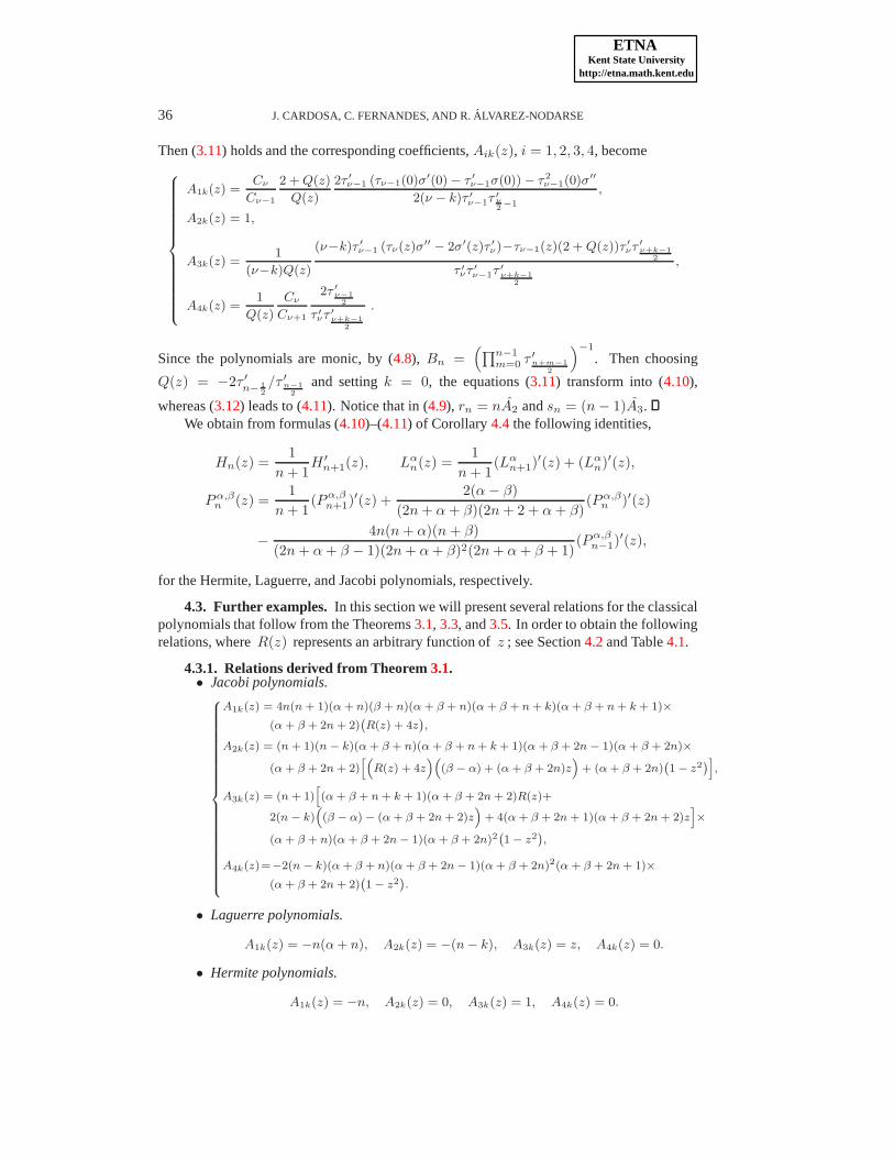
36 J. CARDOSA, C. FERNANDES, AND R.ALVAREZ-NODARSE
Then (3.11) holds and the corresponding coefficients,Aik(z), i = 1, 2, 3, 4, become
8
>
>
>
>
>
>
>
>
>
>
>
>
>
<
>
>
>
>
>
>
>
>
>
>
>
>
>
:
A1k(z) =Cν
Cν−1
2 + Q(z)
Q(z)
2τ ′ν−1 (τν−1(0)σ
′(0) − τ ′ν−1σ(0)) − τ 2
ν−1(0)σ′′
2(ν − k)τ ′ν−1τ
′ν2−1
,
A2k(z) = 1,
A3k(z) =1
(ν−k)Q(z)
(ν−k)τ ′ν−1 (τν(z)σ′′
− 2σ′(z)τ ′ν)−τν−1(z)(2 + Q(z))τ ′
ντ ′ν+k−1
2
τ ′ντ ′
ν−1τ′ν+k−1
2
,
A4k(z) =1
Q(z)
Cν
Cν+1
2τ ′ν−12
τ ′ντ ′
ν+k−12
.
Since the polynomials are monic, by (4.8), Bn =(
∏n−1m=0 τ ′
n+m−12
)−1
. Then choosing
Q(z) = −2τ ′
n− 12/τ ′
n−12
and settingk = 0, the equations (3.11) transform into (4.10),
whereas (3.12) leads to (4.11). Notice that in (4.9), rn = nA2 andsn = (n − 1)A3.We obtain from formulas (4.10)–(4.11) of Corollary4.4the following identities,
Hn(z) =1
n + 1H ′
n+1(z), Lαn(z) =
1
n + 1(Lα
n+1)′(z) + (Lα
n)′(z),
Pα,βn (z) =
1
n + 1(Pα,β
n+1)′(z) +
2(α − β)
(2n + α + β)(2n + 2 + α + β)(Pα,β
n )′(z)
−4n(n + α)(n + β)
(2n + α + β − 1)(2n + α + β)2(2n + α + β + 1)(Pα,β
n−1)′(z),
for the Hermite, Laguerre, and Jacobi polynomials, respectively.
4.3. Further examples. In this section we will present several relations for the classicalpolynomials that follow from the Theorems3.1, 3.3, and3.5. In order to obtain the followingrelations, whereR(z) represents an arbitrary function ofz ; see Section4.2and Table4.1.
4.3.1. Relations derived from Theorem3.1.• Jacobi polynomials.
8
>
>
>
>
>
>
>
>
>
>
>
>
>
>
>
>
>
>
>
>
>
>
<
>
>
>
>
>
>
>
>
>
>
>
>
>
>
>
>
>
>
>
>
>
>
:
A1k(z) = 4n(n + 1)(α + n)(β + n)(α + β + n)(α + β + n + k)(α + β + n + k + 1)×
(α + β + 2n + 2)`
R(z) + 4z´
,
A2k(z) = (n + 1)(n − k)(α + β + n)(α + β + n + k + 1)(α + β + 2n − 1)(α + β + 2n)×
(α + β + 2n + 2)h“
R(z) + 4z”“
(β − α) + (α + β + 2n)z”
+ (α + β + 2n)`
1 − z2´
i
,
A3k(z) = (n + 1)h
(α + β + n + k + 1)(α + β + 2n + 2)R(z)+
2(n − k)“
(β − α) − (α + β + 2n + 2)z”
+ 4(α + β + 2n + 1)(α + β + 2n + 2)zi
×
(α + β + n)(α + β + 2n − 1)(α + β + 2n)2`
1 − z2´
,
A4k(z)=−2(n − k)(α + β + n)(α + β + 2n − 1)(α + β + 2n)2(α + β + 2n + 1)×
(α + β + 2n + 2)`
1 − z2´
.
• Laguerre polynomials.
A1k(z) = −n(α + n), A2k(z) = −(n − k), A3k(z) = z, A4k(z) = 0.
• Hermite polynomials.
A1k(z) = −n, A2k(z) = 0, A3k(z) = 1, A4k(z) = 0.

ETNAKent State University
http://etna.math.kent.edu
RECURRENCE RELATIONS FOR HYPERGEOMETRIC-TYPE FUNCTIONS 37
4.3.2. Relations derived from Theorem3.3.• Jacobi polynomials.
8
>
>
>
>
>
>
>
>
>
>
>
>
>
>
>
>
>
>
>
>
>
>
>
>
<
>
>
>
>
>
>
>
>
>
>
>
>
>
>
>
>
>
>
>
>
>
>
>
>
:
A1k(z) = 4n(n + 1)(α + n)(β + n)(α + β + n)(α + β + n + k + 1)×
(α + β + 2n + 2)`
R(z) + 4z´
,
A2k(z) = −(n − k)(α + β + n)(α + β + n + k + 1)(α + β + 2n − 1)(α + β + 2n)×
(α + β + 2n + 2)h
R(z)(α + β + 2n) + 2“
(β − α) + (α + β + 2n − 2)z”i
,
A3k(z) = (α + β + n)(α + β + 2n − 1)(α + β + 2n)“
(β − α) − (α + β + 2n)z”
×
h
2(n − k)“
(β − α) − (α + β + 2n + 2)z”
− (α + β + 2n + 2)ד
(α + β + n + k + 1)R(z) − 4(α + β + 2n)z”i
,
A4k(z)=−(n − k)(α + β + n)(α + β + 2n − 1)(α + β + 2n)(α + β + 2n + 1)×
(α + β + 2n + 2)“
(β − α) − (α + β + 2n)z”
.
• Laguerre polynomials.
A1k(z) = −n(α + n), A2k(z) = n − k, A3k(z) = −(α + n − z), A4k(z) = 0.
• Hermite polynomials.
A1k(z) = −n, A2k(z) = −2(n − k), A3k(z) = 2, A4k(z) = 0.
4.3.3. Relations derived from Theorem3.5.• Jacobi polynomials.
8
>
>
>
>
>
>
>
>
>
>
>
>
>
>
>
>
<
>
>
>
>
>
>
>
>
>
>
>
>
>
>
>
>
:
A1k(z) = 4n(n + 1)(α + n)(β + n)(α + β + n)(α + β + n + k)(α + β + n + k + 1)×
(α + β + 2n + 2)“
R(z) +`
α + β + 2n + 1´
”
,
A2k(z) = (n − k)(n + 1)(α + β + n)(α + β + n + k + 1)(α + β + 2n − 1)(α + β + 2n)×
(α + β + 2n + 1))h“
(β − α) + (α + β + 2n)z”
(α + β + 2n + 2) − 2(β − α)R(z)i
,
A3k(z) = −(n + 1)(α + β + n)(α + β + 2n − 1)(α + β + 2n)2(α + β + 2n + 1)×
(α + β + 2n + 2)“
R(z) + (α + β + n + k + 1)”
`
1 − z2´
,
A4k(z)=−2R(z)(n − k)(n − k + 1)(α + β + n)(α + β + 2n − 1)(α + β + 2n)2×(α + β + 2n + 1)(α + β + 2n + 2).
• Laguerre polynomials.
A1k(z) = n(α + n), A2k(z) = n − k, A3k(z) = −z, A4k(z) = 0.
• Hermite polynomials.
A1k(z) = n, A2k(z) = 0, A3k(z) = −1, A4k(z) = 0.
4.3.4. A known identity for the Laguerre polynomials. To conclude this paper, wederive a very well-known formula for the Laguerre polynomials using the method describedhere. Puttingk = 0 in relations (3.19)–(3.20), for the Laguerre polynomials, we obtain
(4.12) A1(x)L(α)n−1(x) + A2(x)L(α)
n (x) + A3(x)(
L(α)n+1(x)
)′
= 0 ,
where, by (4.7), the coefficients,Ai, i = 1, 2, 3, are given by
A1(x) = α + n, A2(x) = x − n, A3(x) = x.
ETNAKent State University
http://etna.math.kent.edu
38 J. CARDOSA, C. FERNANDES, AND R.ALVAREZ-NODARSE
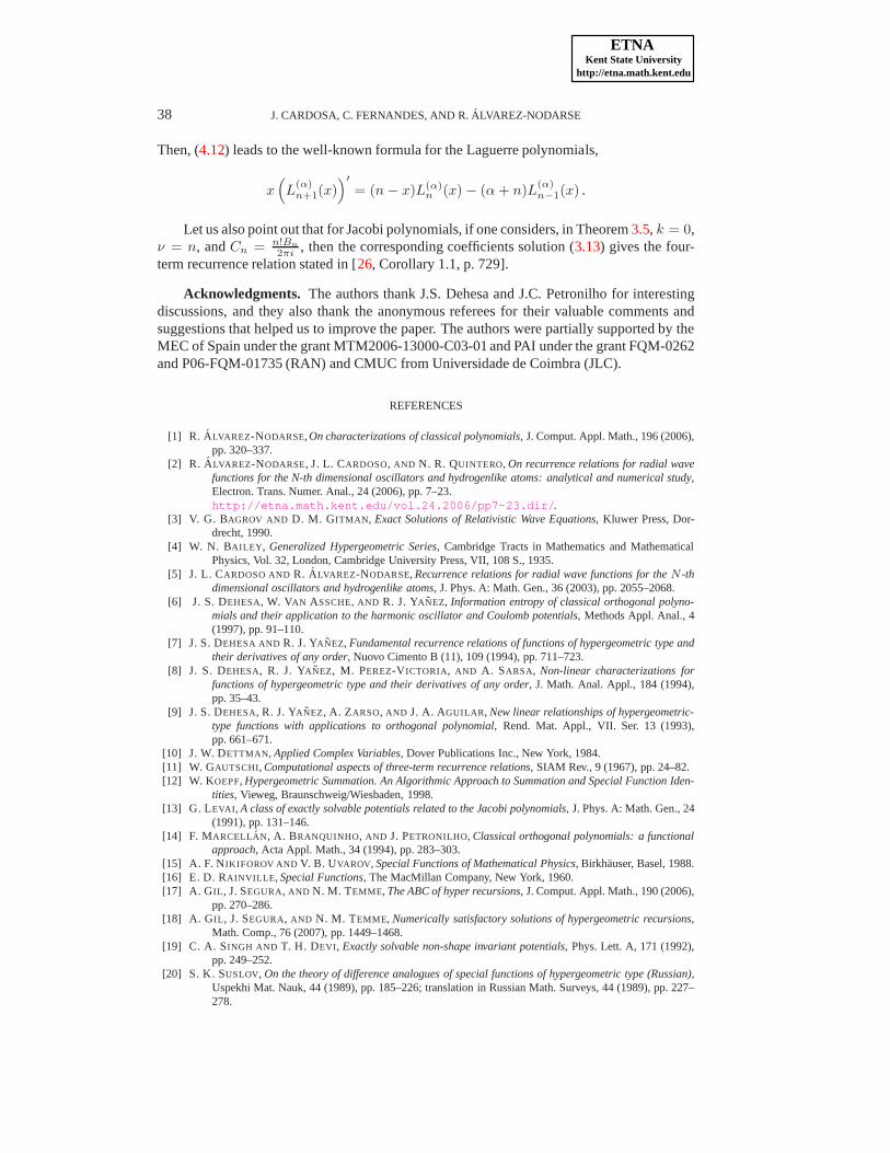
Then, (4.12) leads to the well-known formula for the Laguerre polynomials,
x(
L(α)n+1(x)
)′
= (n − x)L(α)n (x) − (α + n)L
(α)n−1(x) .
Let us also point out that for Jacobi polynomials, if one considers, in Theorem3.5, k = 0,ν = n, andCn = n!Bn
2πi, then the corresponding coefficients solution (3.13) gives the four-
term recurrence relation stated in [26, Corollary 1.1, p. 729].
Acknowledgments. The authors thank J.S. Dehesa and J.C. Petronilho for interestingdiscussions, and they also thank the anonymous referees fortheir valuable comments andsuggestions that helped us to improve the paper. The authorswere partially supported by theMEC of Spain under the grant MTM2006-13000-C03-01 and PAI under the grant FQM-0262and P06-FQM-01735 (RAN) and CMUC from Universidade de Coimbra (JLC).
REFERENCES
[1] R. ALVAREZ-NODARSE,On characterizations of classical polynomials, J. Comput. Appl. Math., 196 (2006),pp. 320–337.
[2] R. ALVAREZ-NODARSE, J. L. CARDOSO, AND N. R. QUINTERO, On recurrence relations for radial wavefunctions for the N-th dimensional oscillators and hydrogenlike atoms: analytical and numerical study,Electron. Trans. Numer. Anal., 24 (2006), pp. 7–23.http://etna.math.kent.edu/vol.24.2006/pp7-23.dir/.
[3] V. G. BAGROV AND D. M. GITMAN , Exact Solutions of Relativistic Wave Equations, Kluwer Press, Dor-drecht, 1990.
[4] W. N. BAILEY , Generalized Hypergeometric Series, Cambridge Tracts in Mathematics and MathematicalPhysics, Vol. 32, London, Cambridge University Press, VII,108 S., 1935.
[5] J. L. CARDOSO AND R. ALVAREZ-NODARSE, Recurrence relations for radial wave functions for theN -thdimensional oscillators and hydrogenlike atoms, J. Phys. A: Math. Gen., 36 (2003), pp. 2055–2068.
[6] J. S. DEHESA, W. VAN ASSCHE, AND R. J. YANEZ, Information entropy of classical orthogonal polyno-mials and their application to the harmonic oscillator and Coulomb potentials, Methods Appl. Anal., 4(1997), pp. 91–110.
[7] J. S. DEHESA AND R. J. YANEZ, Fundamental recurrence relations of functions of hypergeometric type andtheir derivatives of any order, Nuovo Cimento B (11), 109 (1994), pp. 711–723.
[8] J. S. DEHESA, R. J. YANEZ, M. PEREZ-V ICTORIA, AND A. SARSA, Non-linear characterizations forfunctions of hypergeometric type and their derivatives of any order, J. Math. Anal. Appl., 184 (1994),pp. 35–43.
[9] J. S. DEHESA, R. J. YANEZ, A. ZARSO, AND J. A. AGUILAR, New linear relationships of hypergeometric-type functions with applications to orthogonal polynomial, Rend. Mat. Appl., VII. Ser. 13 (1993),pp. 661–671.
[10] J. W. DETTMAN, Applied Complex Variables,Dover Publications Inc., New York, 1984.[11] W. GAUTSCHI, Computational aspects of three-term recurrence relations, SIAM Rev., 9 (1967), pp. 24–82.[12] W. KOEPF, Hypergeometric Summation. An Algorithmic Approach to Summation and Special Function Iden-
tities, Vieweg, Braunschweig/Wiesbaden, 1998.[13] G. LEVAI , A class of exactly solvable potentials related to the Jacobipolynomials, J. Phys. A: Math. Gen., 24
(1991), pp. 131–146.[14] F. MARCELLAN , A. BRANQUINHO, AND J. PETRONILHO, Classical orthogonal polynomials: a functional
approach, Acta Appl. Math., 34 (1994), pp. 283–303.[15] A. F. NIKIFOROV AND V. B. UVAROV, Special Functions of Mathematical Physics,Birkhauser, Basel, 1988.[16] E. D. RAINVILLE , Special Functions,The MacMillan Company, New York, 1960.[17] A. GIL , J. SEGURA, AND N. M. TEMME, The ABC of hyper recursions, J. Comput. Appl. Math., 190 (2006),
pp. 270–286.[18] A. GIL , J. SEGURA, AND N. M. TEMME, Numerically satisfactory solutions of hypergeometric recursions,
Math. Comp., 76 (2007), pp. 1449–1468.[19] C. A. SINGH AND T. H. DEVI, Exactly solvable non-shape invariant potentials, Phys. Lett. A, 171 (1992),
pp. 249–252.[20] S. K. SUSLOV, On the theory of difference analogues of special functions of hypergeometric type (Russian),
Uspekhi Mat. Nauk, 44 (1989), pp. 185–226; translation in Russian Math. Surveys, 44 (1989), pp. 227–278.
ETNAKent State University
http://etna.math.kent.edu
RECURRENCE RELATIONS FOR HYPERGEOMETRIC-TYPE FUNCTIONS 39
[21] A. G. USHVERIDZE, Quasi-Exactly Solvable Models in Quantum Machanics, Institute of Physics, Bristol,1994.
[22] J. WU AND Y. A LHASSID, The potential groups and hypergeometric differential equations, J. Math. Phys.,31 (1990), pp. 557–562.
[23] B. W. WILLIAMS , A second class of solvable potentials related to the Jacobi polynomials, J. Phys. A: Math.Gen., 24 (1991), pp. L667–L670.
[24] J. WIMP, Computation with Recurrence Relations, Applicable Mathematics Series, Pitman Advanced Pub-lishing Program, Boston, MA, 1984.
[25] R. J. YANEZ, J. S. DEHESA, AND A. F. NIKIFOROV,The three-term recurrence relations and the differenti-ation formulas for hypergeometric-type functions, J. Math. Anal. Appl., 188 (1994), pp. 855–866.
[26] R. J. YANEZ, J. S. DEHESA, AND A. ZARZO, Four-term recurrence relations of hypergeometric-type poly-nomials, Nuovo Cimento B (11), 109 (1994), pp. 725–733.
[27] A. ZARZO, R. J. YANEZ, AND J. S. DEHESA, General recurrence and ladder relations of hypergeometric-type functions, J. Comput. Appl. Math., 207 (2007), pp. 166–179.