EU Trade Policies: Benchmarking Protection in a General Equilibrium Framework Alessandro Antimiani (INEA, Italy) and Luca Salvatici (University of Molise, Italy)

Working Paper 05/04 TRADEAG is a Specific Targeted Research Project financed by the European Commission within its VI Research Framework. Information about the Project, the partners involved and its outputs can be found at http://tradeag.vitamib.com

University of Dublin Trinity College

2

EU Trade Policies: Benchmarking Protection in a General Equilibrium

Framework°°°°

Alessandro Antimiani – National Institute of Agricultural Economics (INEA), Italy

Luca Salvatici – University of Molise, Italy

ABSTRACT

This paper deals with the EU’s trade policy with two objectives: on the one hand, we study

the performance of EU's preferential agreements in granting their partners improved market

access; on the other hand, we assess the extent to which domestic sectors are effectively

protected. As far as the first objective is concerned, we construct bilateral indicators of

protection based on the applied tariffs faced by each exporter. In order to do this, an index of

trade policy restrictiveness is computed, using the Mercantilistic Trade Restrictiveness Index

as the tariff aggregator. We also analyze the protection granted to each sector by the existing

tariff structure. In this respect, we compute effective rates of protection that overcome the

well-known theoretical shortcomings of the traditional definition (Output Effective Rate of

Protection).

The analysis is based on a comparative static applied general equilibrium model (Global

Trade Analysis Project) and on the most recent version (release 6) of the related database.

Results are obtained with reference to the situation existing in 2001, but the assessment of

protection is carried out for the enlarged EU. Overall, it appears that notwithstanding the

rhetoric about preferential access, several developing countries are the ones facing the highest

hurdles in getting into the EU markets. Both bilateral protection and effective protection rates

are broadly consistent with the evolution of the WTO negotiations: the strongest demands

from developing countries in terms of market access in the EU have less to do with the overall

applied MFN tariffs on industrial products than the reduction of distortions affecting trade in

agriculture.

Keywords: Protection, Commercial policy, GTAP model, International trade,

JEL classification: F13, Q17, F17

° The authors are solely responsible for the contents of this paper. This work was in part financially supported by

the “Agricultural Trade Agreements (TRADEAG)” project, funded by the European Commission (Specific

Targeted Research Project, Contract no. 513666); and in part supported by the Italian Ministry of University and

Technological Research (“The new multilateral trade negotiations within the World Trade Organisation (Doha

Round): liberalisation prospects and the impact on the Italian economy”).

3

Europe’s Trade Policies: Benchmarking Protectionism in a General Equilibrium Framework

Alessandro Antimiani – Luca Salvatici∗

1. INTRODUCTION

Even after the implementation of the Uruguay Round, trade peaks are still numerous and the

number of preferential trade arrangements (PTAs) surged during the nineties. Tariff

escalation, i.e. higher import duties on processed products than on their input commodities, is

one of the objects of controversy between developed and developing countries. Moreover,

access of developing countries to the markets of developed ones, and particularly of the EU,

mostly occurs through preferential agreements. In this context, we want to provide an

assessment of access to the European market by taking into account both tariff escalation and

preferential agreements.

The evaluation of the levels of protection is a challenging task. International trade policies are

often compared across countries and over time, using such measures as arithmetic or trade-

weighted average tariffs, price wedges and measures of tariff dispersion. But all such

measures are without theoretical foundation. In this paper we assess EU’s trade stance using

two theoretically-based index numbers of trade policy, which provides a true benchmark

against which all these ad hoc measures can be evaluated.

The first one – the Mercantilistic Trade Restrictiveness Index (MTRI) – focuses on the

distortions imposed on the import bundle, using the aggregate import value as the relevant

equivalence criteria. The second one – the Output Effective Rate of Protection (OERP) –

looks at the effects on the production structure, using the sectoral output as benchmark. We

are not aware of any empirical applications of the latter index, originally proposed by

Anderson (1998). As far as the MTRI is concerned, Kee, Nicita and Olarreaga (2005)

compute the index at the bilateral level, but in a partial equilibrium framework. Another

partial equilibrium implementation of the MTRI is provided by Bureau and Salvatici (2005).

The original application by Anderson and Neary (2003) is based on a CGE, but it does not

include the EU. We calculate the MTRI for a cross section of the main EU trading partners

∗ Corresponding author. Mail Address: Dipartimento SEGES, Università degli Studi del Molise, Via De Sanctis,

Campobasso (Italy). Tel.: +39-0874-404240; fax: + 39-0874-311124. E-mail address: luca.salvatici@unimol.it.

4

using the Global Trade Analysis Project model (Hertel, 1997); the same model and data is

used to calculate the OERP for a cross section of EU economic sectors.

The outline of the paper is as follows. Section 2 provides some background on the EU trade

policy. Section 3 introduces the indices that are going to be used for the assessment of the EU

policy – MTRI and OERP. Section 4 details the specification of the model. Section 5 presents

the results, while Section 6 concludes.

2. EU’S “SPAGHETTI BOWL” OF TRADE AGREEMENTS

Economic and trade cooperation have played an integral part of the European policy towards

developing countries since the establishment of the European Community. The EU is

presently engaged in a web of cooperative relations with other countries or regional

groupings, based upon either formal, institutional dialogue or more informal agreements.

Inter-regional cooperation has increased in both the scope and density of the agreements.

Although often controversial, the Euro-Mediterranean process, the EU-Mercosur negotiations

and the Cotonou Agreements constitute examples of this type of attitude.

The EU’s categorization of partners establishes ‘concentric circles’, each circle having a

different intensity of preferences, reciprocity and co-operation instruments. These circles

range from the core integration among the 25 members until the most distant circle where

most-favoured-nation (MFN) treatment is applied according to the WTO.1 Between these two

extremes there are the trade regimes applied to the European Economic Area (Norway,

Iceland and Liechtenstein)2 and Switzerland; the Mediterranean partners (the Euro-Med

agreements); the Africa, Caribbean and Pacific (ACP – formerly the Lomè Convention, now

the Cotonou Agreement) regime; the Everything But Arms (EBA) preferences for least-

developed countries (LDCs); the bilateral free trade areas with Mexico, South Africa and

Chile, plus the ongoing negotiations with Mercosur; the Generalyzed System of Preferences

(GSP) for all developing countries.

The Euro-Mediterranean Agreements: the current set of policies applied to 10 Mediterranean

partners was agreed at the 1995 Barcelona Conference, which launched the Euro-

Mediterranean partnership. The goal is to establish a Free Trade Area by 2010. The Bilateral

1 Between the EU major trading partners, the MFN clause is only applied to USA, Canada, Australia, New

Zealand and Japan. 2 The European Economic Area was created in 1994 to integrate those western European countries that wished to

benefit from the Single Market while remaining outside the EU, although implementation was largely overtaken

by the 1995 enlargement.

5

Euro-Mediterranean Association Agreements are a first step in this direction. Some of these

agreements provide for non-reciprocal free access for non-sensitive products into the EU

market and progressive liberalization for other products.

Cotonou Partnership: Cotonou Partnership Agreements include preferences and linkages

between trade and financial assistance to ACP countries. It covers over 70 countries, which

were mostly former colonies of the EU members. The agreements follow a series of Lomé

Convention arrangements which provide non-reciprocal trade benefits in 99 percent of the

industrial goods and some agricultural products, where political and colonial ties appear as the

major motivation. Under the Cotonou Agreement current non-reciprocal “Lomè” preferences

will be maintained temporarily up 2008 and new reciprocal Economic Partnership

Agreements will be negotiated and implemented gradually.

Bilateral Agreements: agreements with Mexico, Chile, and South Africa provide for

progressive mutual liberalisation of goods and services, although free trade in agriculture and

fisheries is not fully reciprocal and it is limited to lists of products. In the case of South

Africa, for example, EU must give duty-free access to 95 percent (only 62 percent in the case

of agriculture) of products by 2010.

GSP Scheme: in 1968, UNCTAD recommended the creation of a GSP and the waiver to allow

such preferences was granted in 1971. The GSP preference scheme provides nonreciprocal

preferences with lower tariffs or completely duty-free access for imports from 178 developing

countries and territories into the EU market. The EU’s revamped GSP, implemented since

April 2005, includes 3 categories of benefits

1. the General Scheme for all developing countries (with 40 percent of products

receiving duty-free access, but with ceilings and graduation criteria that eliminate

largest exporters);

2. the EBA initiative for Least Developed Countries grants duty-free access on all

products – with the exception of imports of fresh bananas, rice, and sugar – to a set of

the poorest nations in the world;

3. the ‘GSP plus’, which provides duty-free access for all products from ‘countries with

special development needs’ that implement international conventions on the

environment, as well as on human and labour rights.

The complexity in EU trade policy comes not only from different regimes but from

heterogeneous tariffs across commodities. One consequences of the dispersion of the tariffs is

the presence of tariff escalation that consists in protecting processed products at higher level

than primary products.

6

Figure 1 - Tariffs escalation in EU: some sectors by MTN classification (2003, MFN, weighetd average)

0

2

4

6

8

10

12

14

16

18F

ruit &

veg

etab

les

Liv

e an

imal

s

Fis

h

Ore

s &

was

te

Tob

acco

Wo

od

, p

ulp

,

pap

er &

furn

iture

Tex

tile

s &

clo

thin

g

Lea

ther

,

rub

ber

,

foo

twea

r

Man

ufa

cture

s

Chem

ical

s

%

Raw Semi-finished Finished

Source: COMTRADE.

In Figure 1 we used the Trains data base and the MTN classification3 to show how tariff

escalation affects EU trade policy.

3. MEASURING TRADE DISTORTION: MARKET ACCESS AND EFFECTIVE PROTECTION

Measures of trade restrictiveness have long been of interest to international economists. Some

of the literature relies on trade intensity measures, e.g., estimating the volume of trade in the

distorted equilibrium relative to that in free trade. The rationale is that such a ratio

summarizes the impact of all trade policy instruments. The problem is that import volume

could be much lower than in free trade either because tariffs are high on inelastic goods or

because though low they are imposed on highly elastic good.

To measure the protection granted by a country’s trade policy regime, one needs to overcome

two important aggregation hurdles: aggregation of different forms of trade policies and

aggregation across goods with very different economic importance. Regarding the first

aggregation problem, one needs to bring all types of trade policy instruments into a common

metric, in most cases an ad valorem equivalent.

In order to solve the second problem using theoretically sound aggregation procedures, it is

necessary to specify the type of information we want to maintain, so that the final number is

7

equivalent to the original multiple data in the dimension we are interested in. According to

Anderson and Neary (1996), a general definition of a policy index is as follows: depending on

a pre-determined reference concept, any aggregate measure is a function mapping from a

vector of independent variables – defined according to the policy coverage – into a scalar

aggregate. The greatest advantage of this approach is that it is theoretically consistent, since

the equivalence is determined according to a fundamental economic structure. Secondly, it

provides unequivocal interpretation of the results, since the definition and properties of these

“equivalence-based” indicators are predetermined .

3.1 Mercantilistic trade restrictiveness index

The MTRI relies on the idea of evaluating trade policy using trade volume as the reference

standard. The interest is in the extent to which trade distortions limit imports from the rest of

the world, so that the aggregation procedure answers the following question: what is the

equivalent uniform tariff that if imposed to home imports would leave aggregate imports

unchanged?

The MTRI is defined by Anderson and Neary (2003) in terms of the uniform tariff τµ that

yields the same volume (at world prices) of tariff-restricted imports as the initial vector of

(non-uniform) tariffs. This can be expressed with import demand functions M, while holding

constant the balance of trade function at level B0:

(1) [ ] ( )0*0000 ,,,,: BppMBppM =µµτ , with ( )µµ τ+≡ 1*pp .

where *p denotes the international prices ( *

kp ) vector of the N goods k = (1,…,N), M0 is the

value of aggregate imports (at world prices) in the reference period, and p0 is the initially

distorted price vector.

Define the scalar import demand as

(2) ( ) ( )∑∑= =

≡r

c

N

k

m

kckc BpIpBppM1 1

,

*

, ,*,,

where m

kcI , denotes the uncompensated (Marshallian) import demand function of good k from

country c. Accordingly, the MTRI uniform tariff τµ would lead to the same volume of imports

(at world prices) as the one resulting from the uneven tariff structure, denoted by the Nxr

bilateral tariffs matrix T whose elements are tc,k:

3 MTN classification aggregates products of a single chapter (2 HS digit) by their level of processing stage: raw,

semi-finished and finished or semi-processed and processed.

8

(3) [ ] [ ]∑∑∑∑= == =

=r

c

N

k

m

kckc

r

c

N

k

m

kckc BpIpBpIp1 1

00

,

*

,

1 1

0

,

*

, ,,µ

The previous definition focuses on the overall distortions imposed by a country’s trade

policies on its import bundle. In the case of bilateral protection indexes, trade restrictiveness

is the product of the structure of protection and the trade flows product specialization. Even if

the EU applied MFN bound tariffs to all exporters, the impact would be differentiated: trade

would be more restricted in the case of countries exporting products facing the highest tariffs.

In order to take into account the trade impact of protection, one could think of using a

bilateral trade-weighted average. As it is well-known, though, this would underestimate the

protection effect, because of the endogeneity bias: actual trade is much lower with high tariffs

than it would be with lower tariffs. On the other hand, using an “equivalence-based” index

with a behavioural underpinning such as the MTRI, the weights depend on import volumes

evaluated at world prices.

In our application, we are interested in calculating the MTRI uniform tariff bilaterally, to

obtain the level of trade restrictiveness that the EU imposes on exports of each country c.

Accordingly, in equation (3), instead of summing over k and c, one would only sum over k to

obtain a bilateral uniform tariff MTRI ( µτ c ) defined as follows:

(4) ( )[ ] 00* ,1: cccc MBpM =+ µµ ττ ,

where 0

cM is the value of aggregate imports (at world prices) from country c in the reference

period.

Finally, in the standard definition prices are assumed fixed on world markets. Anderson and

Neary (2003), argue (footnote 8) that “there is a rationale for a ceteris paribus trade

restrictiveness index that fixes world prices even when these prices are in fact endogenous”.

Such a rationale may be represented by the fact that, by keeping world prices constant, we

focus on the component of protection explained by national policies, and not by the degree of

market power of the country.

Nonetheless, we need to recast the definition of the MTRI in order to make it consistent with

the model used for the assessment of the EU trade policy. Since the GTAP model is a global

one with endogenous world prices, the terms of trade impact needs to be considered. In order

to compute the MTRI with the GTAP model, we redefine the uniform tariff equivalent

relaxing the small country assumption. The vector of world prices p* is a function of tariffs T.

To accommodate this, the definition of the MTRI [see equation (4)] is modified as follows

(5) ( ) ( )[ ] 00* ,1: c

w

cc

w

c MBTpM =+ττ ,

9

where ( w

cτ ) is the bilateral MTRI uniform tariff with endogenous world prices.

In the case of τµ, totally differentiating (1) to derive the effects of tariff changes, holding p*

and B0

fixed, gives:

(6) µµµ

µ

τ

τ

pM

dpMd

p

p

00

1=

+.

With endogenous world prices ( ** tdpdtpdp += ), we get

(7) ( )w

ww

p

p

ww

p

p

w

w

tpM

dpM

pM

dtpMdτ

τ

τΦ−+=

+

0

*00*0

1, where

*0

*

dpM

dpM

p

w

p≡Φ .

φ is a correction factor, which is needed because the import volume function is evaluated at

two different points (denoted by superscripts): the initial tariff-distorted price vector p0 and

the uniform-tariff-equivalent price vector ( )ww pp τ+≡ 1* . Comparing (6) and (7) it appears

that τw could be either larger or smaller than τµ.

3.2 Output effective rate of protection

The EU tariff structure, as well as that of many other developed countries, not only presents a

large dispersion of tariffs across commodities, but it is also characterized by tariff escalation

since tariffs are generally higher on processed products than on inputs (see section 2). Tariff

escalation refers to the wedge between tariffs on processed commodities and those levied on

the inputs used in the production process. Tariff wedges can be readily computed only if we

do not face production functions with multiple inputs and/or outputs. More generally, in order

to compare the protection given to different sectors of the economy, we cannot rely on

‘nominal wedges’ (Lindland, 1997). We need to compute an effective rate of protection, that

is an index which, focusing on gross (rather than net) output, is able to take into account the

role of the protection provided to the intermediate inputs.

Similarly to the measurement of nominal protection, effective protection can be defined as the

proportional increase in the price of a sector’s gross output relative to free trade. Since the

total value of gross output priced at value added per unit equals the total value of net output

valued at equilibrium prices, an appropriate price for gross output is the value-added per unit

(Corden, 1971). Accordingly, the effective rate of protection (ERP) of industry j (Ej) measures

the increase in industry’s value added per unit of output under protection (Vj’) as a percentage

of the free trade value added per unit (Vj):

10

(8) j

jj

jV

VVE

−=

'

.

Assuming that one unit of output j necessitates the use of aij quantity of inputs i, we can write:

(9) ( ) ( )∑

∑

+−+=

−=

i

iijjj

i

ijj

tpatpV

papV

ij

ij

11 **'

**

If **

jippac ijij = is the cost share of input i in output j, after simplification we get:

(10) ∑

∑

−

−

=−

=

i

ij

i

iijj

j

jj

jc

tct

V

VVE

1

'

.

The traditional definition of the ERP is based on restrictive assumptions (fixed coefficient

and/or separability) regarding the production functions (Anderson and Naya, 1969). If the

assumption of fixed physical input coefficients does not hold, free trade input-output

coefficients must be inferred from the observed distorted coefficients (Bureau and

Kalaitzandonakes, 1995).

The fundamental theoretical critique moved to the effective protection concept stems largely

from concerns about drawing general equilibrium inferences from a partial equilibrium

measure (Ethier, 1971, 1977; Bhagwati and Srinivasan, 1973; Davis, 1998). The development

of the concept of effective protection, as a matter of fact, may be seen as an attempt to define

the index as a pure production concept – expressed in terms of nominal prices and input

coefficient – making enough assumptions so that demand might be ignored: “Effective

protection is the ranch house of trade policy construction – ugly but apparently too useful to

disappear” (Anderson, 1998).

Also in terms of the possibility for the ERP to be a good predictors of gross outputs change,

effective protection is a partial equilibrium index, since in reality the prices of primary (non-

produced) factors are endogenous, and the prices of (internationally) non-traded goods may

change as well. As a consequence, even if the fixed coefficient assumption is met, ranking

effective rates may not allow ranking percentage output changes: a non-prohibitive import

tariff or export tax in partial equilibrium might become prohibitive in general equilibrium

(Anderson, 1970).

Nowadays, the development of computable general equilibrium models implies that ERPs can

be computed as a general equilibrium index summarising all the model information (Stevens,

1996). In this perspective, Anderson (1998) suggested an interesting new definition of the

11

index: the distributional effective rate of protection, based on the uniform tariff which is

equivalent to the actual differentiated tariff structure in its effects on the rents to residual

claimants in a given sector.

The same approach can be used to define an index which is able to measure the impact of

protection on the ability of sectors to compete with other industries in factor markets: the

Output Effective Rate of Protection (OERP). This index is based on the uniform tariff on all

distorted sectors which produces the same level of output, sector by sector, as does the initial

differentiated tariff structure (Anderson, 1998). Output variations across sectors reflect both

the structure of protection (which the old effective protection concept tried to measure) and

differences in the production structure of the economy. The two questions, ‘how much

protection is given’ and ‘how much does supply change as a result’ are distinct, and the

OERP gives a precise answer to the latter.

The output effective rate of protection ej of sector j in general equilibrium is defined as the

uniform tariff which exert on the output of j an effect which is equivalent to the initial tariff

structure. That is

(11) ( )[ ] ( )000 ,,,: wpYvpwpYe j

e

j

ee

jjj = , with ( )jj

e

j epp +≡ 1* .

where Yj is j supply function, and w is the vector of competitive factor prices (w is function of

the price vector p and of the fixed factor supply v).

The previous definition is based on the "small country" assumption. If we want to allow for

endogenous world prices, we need to define the vector p* as a function of the tariff vector (t).

Equation (11) becomes:

(12) ( ) ( ) ( ) ( )( )[ ] ( ) ( ) ( ) ( )( )( )[ ]vtptwtptYvtpewtpeYe jjjjjj

we

j

w

j

w

jjj,1,1,1,1: *00*00** ++=++ ,

where ( w

je ) is the OERP uniform tariff with endogenous world prices.

4. COMPUTATION OF THE INDICES WITH AN APPLIED GENERAL EQUILIBRIUM MODEL

4.1 GTAP model and database

We use the GTAP model of global trade (version 6.2). GTAP is a static, multi-region, general

equilibrium model which includes explicit treatment of international trade and transport

margins, a “global” bank designed to mediate between world savings and investment, and a

consumer demand system designed to capture differential price and income responsiveness

across countries. As documented in Hertel (1997) and on the GTAP web site (www.gtap.org),

12

the model includes: demand for goods for final consumption (based on a Constant Difference

of Elasticity functional form), intermediate use and government consumption, demands for

factor inputs (based on a Constant Elasticity of Substitution functional form), supplies of

factors and goods, and international trade in goods and services.

The model employs the simplistic but robust assumptions of perfect competition and constant

returns to scale in production activities. Bilateral international trade flows are handled using

the Armington assumption by which products are exogenously differentiated by origin

(Armington, 1969). In the standard closure case, global investment adjusts to global saving,

so that national balances of payments are endogenous.

The latest version of GTAP database, version 6, provides a baseline for year 2001. It includes

up to a maximum of 87 regions and 57 sectors. Trade policy is set at the tariff line level, but

this implies a level of detail that is not consistent with the GTAP (or any other existing)

model: the EU tariff schedule, for example, includes more than 10000 tariff lines. To reach

consistency between trade distortions and model aggregation, a-theoretic trade weighted

average tariffs are used, losing considerable information.

On the other hand, it should be noted that the quality of the trade distortion data included in

the version 6 of the GTAP database is much better than in the previous release due to the use

of the MacMap-HS6 (version 1), a database at the HS-6 level intended to provide a set of

consistent and exhaustive ad valorem equivalents (AVEs) of applied border protection across

the world.4 This resulted in considering applied/preferential tariffs rather than bound ones,

and in a more accurate computation of the AVE for each trade instrument (Bouët et al., 2005).

Specific tariffs were converted in AVE terms by dividing the duty by a unit value. The whole

problem lies in the choice of this unit value, a rather sensitive issue both from a theoretical

and from a political point of view (as the recent evolution of WTO negotiations shows). This

has led to base AVE calculations on the median unit value of worldwide exports originating

from a reference group the exporter belongs to.5

In the case of mixed tariffs, i.e. tariffs involving a choice (a maximum or a minimum

operator) between various terms, the choice is made as follows:

• when the tariff is defined as an ad valorem base tariff, the base tariff is retained. If the

base tariff is in specific terms and the cap and the floor are ad valorem, a simple

average of the two bounds is retained;

4 MAcMap-HS6 is regularly improved and updated, and the corresponding information is available on the

CEPII's website (www.cepii.fr).

13

• when the tariff involves choosing between two terms, priority is given to ad valorem

tariffs.

Regarding tariff rate quotas (TRQs), three market regimes are considered, depending on the

level of the fill rate:

• if the fill rate is less than 90% (quota not binding), the inside quota tariff rate is chosen

as the applied rate;

• in the (90%–99%) range (quota assumed to be binding), a simple arithmetic average is

used;

• if it is higher than 99% (quota binding), the applied rate is equal to the outside quota

tariff rate.

Finally, the presence of prohibitive tariffs is problematic when calculating AVEs. Therefore,

an upper limit to the AVE is established starting at the HS6 level: the limit is set to 1,000%

for the sum of all instruments.

We use two different regional aggregations, one for the computation of MTRI and one for the

OERP, while the fairly detailed sector aggregation (43 products)6 is the same in both cases

(Table 1). The difference in the regional aggregations is explained to by the different

objectives of our analysis.

In the case of the MTRI, we look at the bilateral protection implied the EU trade policy. As a

consequence, we singled out 18 regions (including a residual aggregate – “rest of the world”)

as EU trading partners. Although the database cannot take into account the 2004 EU

enlargement, we consider an enlarged EU (EU25) building a counterfactual baseline where

the enlargement would have taken place in 2001 (Antimiani, Conforti, Salvatici, 2003).

Accordingly, we eliminated all trade barriers and export subsidies between EU members and

we extended the EU trade policy to the new members.

5 These groups are defined on the basis of a hierarchical clustering analysis based on GDP per capita (in terms of

PPP) and trade openness. 6 We do not exploit the maximum level of detail allowed by the database (57 sectors), since 14 sectors (services)

are not associated with any protection rates.

Table 1 - GTAP sectoral and regional aggregations used

Sectors Factors MTRI regional aggregation OERP regional aggregation

Paddy rice Land (sluggish) Eu25 Eu25

Wheat Unskilled labour (mobile) Candidates (Bulgary and Romania) Rest of the World (Row)

Other cereals Skille labour (mobile) Efta (European free trade area)

Vegetables and fruit Capital (mobile) Balkans

Oil seeds Natural resources (sluggish) ACP countries

Sugar can and beet USA

Plant based fibers Canada

Other crops Australia

Livestock: cattle, sheep, goats and horses Japan

Other live animals China

Raw milk India

Wool and silk Mexico

Forestry Argentina

Fishing Brazil

Coal Russian Federation

Oil Turkey

Gas Morocco

Other natural resources Tunisia

Meat : cattle, sheep, goats and horses Rest of the World (Row)

Other meat

Vegetables oils and fats

Dairy products

Processed rice

Sugar

Other food products

Beverages and tobacco

Textile

Wearing products

Leather products

Wood products

Paper and publishing

Petroleum and coal products

Chemical, rubber and plastic products

Other minerals

Ferrous metals

Other metals

Metal products

Motor vehicles and parts

Transport equipment

Electronic equipment

Other machinery and equipment

Other manufactures

Services

In the case of the OERP, we want to assess the effective protection provided to different

sectors. This does not require a detailed regional aggregation, so we only consider 2 regions:

the EU25 and the rest of the world. Also in this case, the baseline assumes that the EU

enlargement had already been implemented.

4.2 MTRI

As far as the regional aggregation is concerned, our choice was obviously driven by the

geographical focus of the EU trade policies presented in Section 2 (Table 2).

Table 2: EU trade policy and model regional aggregation

REGIONAL AGREEMENTS

Turkey Customs union (industrial products)

Bulgaria, Romania Candidates to accession

Efta (Iceland, Norway, Liechtenstein and Switzerland) Free trade area

PREFERENTIAL AGREEMENTS

Acp (Botswana, South Africa, Malawi, Mozambique, Tanzania, Zambia,

Zimbabwe, Madagascar, Uganda)Cotonou Partnership

Morocco, Tunisia, Algeria, Egypt, Israel, Jordan, Lebanon, Syria and

Palestinian AuthorityEuro-Mediterranean Agreements

Balkans (Croatia, Albania, Rep. Of Macedonia and Former Yugoslav) Stability and Association Agreements

India, China GSP

TO BE IMPLEMENTED

Argentina Mercosur negotiations

Mexico, Chile Bilateral agreements

MFN

Usa, Canada, Australia, Japan WTO membership

OTHER

Russia Cooperation Agreements

It is worth recalling that many regional and preferential agreements allow for long

implementation periods and were not in place in 2001: this explains, for example, why there

is not an “EBA group” and South-Africa is not singled out as a free-trade partner. Moreover,

the choice of the countries to be included in our analysis takes into account the relevance of

EU bilateral trade flows (Figure 2).

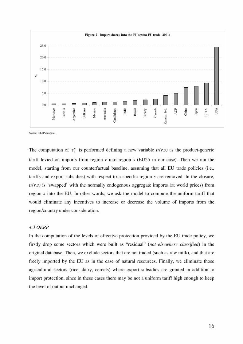
16

Figure 2 - Import shares into the EU (extra-EU trade, 2001)

0,0

5,0

10,0

15,0

20,0

25,0

Mo

rocc

o

Tunis

ia

Arg

enti

na

Bal

kan

s

Mex

ico

Aust

ralia

Can

did

ates

India

Bra

zil

Turk

ey

Can

ada

Russ

ian f

ed.

AC

P

Ch

ina

Japan

EF

TA

US

A

%

Source: GTAP database.

The computation of w

cτ is performed defining a new variable tr(r,s) as the product-generic

tariff levied on imports from region r into region s (EU25 in our case). Then we run the

model, starting from our counterfactual baseline, assuming that all EU trade policies (i.e.,

tariffs and export subsidies) with respect to a specific region s are removed. In the closure,

tr(r,s) is ‘swapped’ with the normally endogenous aggregate imports (at world prices) from

region s into the EU. In other words, we ask the model to compute the uniform tariff that

would eliminate any incentives to increase or decrease the volume of imports from the

region/country under consideration.

4.3 OERP

In the computation of the levels of effective protection provided by the EU trade policy, we

firstly drop some sectors which were built as “residual” (not elsewhere classified) in the

original database. Then, we exclude sectors that are not traded (such as raw milk), and that are

freely imported by the EU as in the case of natural resources. Finally, we eliminate those

agricultural sectors (rice, dairy, cereals) where export subsidies are granted in addition to

import protection, since in these cases there may be not a uniform tariff high enough to keep

the level of output unchanged.

17

Table 3 - Sectors for the OERP calculation

Vegetables and fruit

Oil seeds

Sugar can and beet

Livestock: cattle, sheep, goats and horses

Forestry

Fishing

Vegetables oil and fats

Other food products

Beverages and tobacco

Textile

Wearing products

Leather products

Wood products

Paper and publishing

Petroleum and coal products

Chemical, rubber and plastic products

Ferrous metals

Metal products

Motor vehicles and parts

Transport equipment

Electronic equipment

Other machinery and equipment

Other manufactures

We are left with a subset of 23 sectors (Table 3) for which we compute the ERP and the

OERP. The traditional index is computed according to equation (10), recalling that the cost

shares are to be evaluated at world prices, and that when some intermediate inputs are not

distorted, the denominator in (10) must be calculated as ‘value added by undistorted inputs’.

The computation of w

je is performed definining a new variable te(s) as the product and

source-generic tariff levied on imports into region s (EU25 in our case). Then, we run the

model, starting from our counterfactual baseline, assuming that all EU trade policies (i.e.,

tariffs and export subsidies) are removed. In the closure, te(s) is ‘swapped’ with the normally

endogenous output supply of sector j of the EU. In other words, we ask the model to compute

the uniform tariff that would eliminate any incentives to increase or decrease the output of the

sector under consideration.

18

5. RESULTS

5.1. Market access

Results for the MTRI bilateral uniform tariffs are presented in Table 4, with the trade-

weighted average tariffs for reference.

Table 4 - EU bilateral MTRI and weighted average tariffs

Trade-weighted average tariff MTRI uniform tariff

EFTA 0,45 0,42

Mexico 0,49 0,95

Canada 0,90 2,09

Morocco 1,09 7,61

Turkey 1,12 2,22

Russian federation 1,29 0,73

USA 1,31 2,25

Australia 1,36 3,94

Balkans 1,49 0,07

Tunisia 1,60 1,86

Candidates 1,61 1,10

Japan 2,81 3,31

ACP 2,98 4,37

India 3,28 10,25

China 3,51 3,93

Argentina 6,56 9,06

Brazil 7,39 24,96 Source: Simulation results.

Table 5 presents the results of a simple regression and rank correlations between the columns

in Table 4, while Figure 3 illustrates the data from Table 4 with countries ranked by their

trade-weighted average tariff.

19

Table 5: Regression Equations Based on Columns in Table 4

Regression

equation

a b r Rank

MTRI on trade-

weighted average

-1.130

(1.327)

2.506

(0.441)

0.826 0.679

Notes: a is the intercept and b the slope coefficient; standard errors are in parentheses; r is the correlation

coefficient; and Rank is the rank correlation coefficient.7

Figure 3 - EU bilateral MTRI and weighted average tariffs

0

5

10

15

20

25

30

EF

TA

Mex

ico

Can

ada

Moro

cco

Turk

ey

Russ

ian f

eder

atio

n

US

A

Aust

ralia

Bal

kan

s

Tunis

ia

Can

did

ates

Japan

AC

P

India

Chin

a

Arg

entina

Bra

zil

%

Trade-weighted average tariff MTRI uniform tariff

Source: Simulation results.

Looking at the MTRI tariff values, it is striking that the most restricted countries in their trade

with the EU are some developing ones. Morocco, Argentina, India present values around

10%, and Brazil even above 20%. These countries have something in common: they face an

EU tariff profile heavily biased against agricultural imports, as it can be seen in Table 6

ranking the ten highest bilateral tariffs reported in the GTAP database.

20

Brazil India

1) Sugar (184.5) 1) Meat (204.7)

2) Meat (112.9) 2) Processed rice (106.2)

3) Rice (96.4) 3) Sugar (59.7)

4) Sugar cane & beet (57.3) 4) Rice (49.7)

5) Dairy products (35.1) 5) Beverages and tobacco (20.2)

6) Meat products (29.4) 6) Dairy products (11.9)

7) Cereal grains (27.5) 7) Cereal grains (8.8)

8) Processed rice (19.7) 8) Leather products (8.5)

9) Food products (14.2) 9) Meat products (8.1)

10) Beverages and tobacco (12.8) 10) Textiles (7.5)

Argentina Morocco

1) Sugar (107.7) 1) Meat (136.4)

2) Dairy products (37.2) 2) Vegetable oils & fats (48.8)

3) Processed rice (34.3) 3) Beverages and tobacco (14.9)

4) Meat (29.6) 4) Sugar (11.9)

5) Cereal grains (28.8) 5) Fruit & vegetables (11.3)

6) Meat products (20.2) 6) Dairy products (11.3)

7) Fruit & vegetables (16.3) 7) Meat products (5.4)

8) Animal products (10.8) 8) Other crops (1.9)

9) Fishing (9.7) 9) Livestocks (1.2)

10) Food products (9.3) 10) Food products (1.1)

Table 6 - Most EU protected sectors in bilateral trade with Brazil, India, Argentina and

Morocco (trade-weighted average tariffs are in parentheses)

Source: Simulation results.

Not surprisingly, then, Brazil, Argentina and India were between the founding members of the

so-called G-20 group, one of the main actor in the present agricultural WTO negotiations,

while Brazil and Argentina are also members of the Cairns Group, another coalition of

countries asking for a substantial liberalization of agricultural trade. In the case of Morocco, it

can be pointed out that it recently signed a free-trade agreement with the USA

notwithstanding the opposition of the EU: such a move took many by surprise, but it could be

explained by the disillusion for the lack of results in terms of actual access to the EU market.

Developed countries facing MFN bound rates – USA, Canada, Australia, Japan – present

values ranging between 2 and 4%. This means that their exports face an overall protection

which is comparable to the one faced by ACP countries – a group with a long tradition of

(supposedly) preferential access into the EU market –, China and Turkey. In the case of ACP,

7 The Rank coefficient is calculated as follows:

( )1

)(

612

1

2

−

−

−=∑

=

nn

RankRank

Rank

n

i

i

tariffAverage

i

tariffMTRI

, with n

21

it is a generally accepted view that these countries, despite benefiting from one of the most

generous trade preference scheme of the EU providing free access for 95% of their exports,

have been unsuccessful in taking advantage of their preferential status (Manchin, 2005).8 The

European Commission itself expressed serious doubts on the benefits of the ACP preferential

regime during the design of the Cotonou agreement (Bureau and Matthews, 2005).

The only countries that seem to enjoy a preferential margin with respect to the major world

exporters are the European ones – EFTA members, candidates to the accession, Balkan

countries – together with Mexico and Russia; the latter result is particularly remarkable, since

Russia is not even a WTO member yet.9

Comparing the columns of Table 4, the first observation is that the MTRI uniform tariff and

the trade-weighted average tend to move together on average. The effect is statistically

significant (as Table 5 shows), though the relation is not a very close one: correlation and

rank correlation coefficients equal to 0.826 and 0.679 respectively.

This result is in line with the findings of Anderson and Neary (2003) and Bach and Martin

(2001) who show that the trade-weighted average tariff is a linear approximation to the tariff

aggregator based on the expenditure function. Anderson and Neary (2003) also prove that the

MTRI uniform tariff is more likely to be higher than the trade-weighted average the more

elastic is the demand for the tariff-constrained imports. Indeed, the trade-weighted average

tariff underpredicts the MTRI uniform tariff in all but four of the seventeen cases. The

difference between the two measures is significant (as Table 5 shows), and of unpredictable

sign in individual cases: the relative difference between the two indexes exceeds 90% on

average, reaching over 150% for India, Brazil and Morocco.

5.2. Effective protection

Results for the OERP uniform tariffs are presented in Table 7, with the ERP and the trade-

weighted averages for reference.

equal to the number of countries considered (19 in our case). 8 Manchin (2005) reports that, despite the number of Lomè beneficiaries increasing over time, the share of EU

imports from the ACP in total EU imports decreased from 6.7% in 1976 to 3.11% in 2002. 9 Indeed, this finding seems to confirm the doubts of those arguing that countries joining or belonging to the

GATT/WTO do not show very different trade patterns than outsiders (Rose, 2004).

22

Table 7 - Effective protection in EU25 by two indexes, ERP and OERP, and weighted average tariffs

Sectors

Weighted

average

tariffs

ERP OERP

Vegetables and fruit 17,06 21,0 31,65

Vegetables oil and fats 11,97 11,5 93,05

Sugar cane and beet 8,69 10,7 198,78

Other food products 8,04 -2,1 40,95

Beverages and tobacco 7,34 0,8 5,19

Motor vehicles and parts 6,07 9,0 -3,62

Leather products 5,49 2,5 20,08

Wearing products 5,35 6,3 10,53

Livestock: cattle, sheep, goats and horses 4,97 1,9 132,76

Textile 4,24 4,8 13,26

Ferrous metals 3,99 5,2 0,69

Fishing 2,47 2,0 4,71

Chemical, rubber and plastic products 1,82 1,2 3,27

Metal products 1,7 1,4 6,6

Transport equipment 1,5 1,0 8,83

Petroleum and coal products 1,21 7,5 -1,91

Other machinery and equipment 1,03 0,6 7,19

Paper and publishing 0,27 0,0 32,05

Forestry 0,06 -0,9 -4,64

Oil seeds 0 -1,1 -6,07 Source: Simulation results.

Table 8 presents the results of a simple regression and rank correlations between the columns

in Table 7, while Figure 4 illustrates the data from Table 7 with sectors ranked by their trade-

weighted average tariff.

23

Table 8: Regression Equations Based on Columns in Table 7

Regression

equation

a b r Rank

OERP on ERP 17.427

(14.501)

2.939

(2.115)

0.311 0.239

OERP on average

tariff

5.371

(16.182)

5.210

(2.559)

0.433 0.579

Notes: a is the intercept and b the slope coefficient; standard errors are in parentheses; r is the correlation

coefficient; and Rank is the rank correlation coefficient.10

Figure 4 - OERP, ERP and weighted average tariffs in EU for some sectors

-200

2040

6080

100120

140160

180200

Veg

etab

les a

nd fr

uit

Veg

etab

les o

il an

d fa

ts

Sugar

can

e an

d be

et

Oth

er fo

od p

rodu

cts

Bev

erag

es and

toba

cco

Mot

or v

ehic

les a

nd p

arts

Leath

er p

rodu

cts

Wea

ring

prod

ucts

Lives

tock

: cat

tle, s

heep

, goa

ts and

hor

ses

Textil

e

Ferro

us m

etals

Fishi

ng

Che

mical

, rub

ber a

nd p

lastic

pro

ducts

Metal

pro

duct

s

Trans

port equ

ipm

ent

Petro

leum

and

coa

l pro

ducts

Oth

er m

achi

nery

and

equ

ipm

ent

Paper

and

pub

lishi

ng

Fores

try

Oil

seed

s

%

Weighted average tariffs

ERP

OERP

Source: Simulation results.

We were able to obtain results for 20 out of the 23 sectors considered: in the case of wood

products, electronic equipments and other manufactures, as a matter of fact, we did not get

any solutions. The most ‘effectively protected’ sectors are by far the agrifood ones both in

terms of primary (sugar, livestock, vegetables and fruit)11

and processed products (vegetable

oils and fats, food products).

10 The Rank coefficient is calculated as follows:

( )1

)(

612

1

2

/

−

−

−=∑

=

nn

RankRank

Rank

n

i

i

averageERP

i

OERP

, with n

equal to the number of sectors considered (20 in our case). 11

It is worth recalling that other agricultural products were not included in the analysis due to the presence of

export subsidies in addition to rather high tariff protection rates.

24

The difference between nominal and OERP rates are particularly striking in the case of sugar

beet and livestock. As far as the former is concerned, it should be recalled that the actual

structure of protection policy is much more complex than the simple tariff-equivalent

considered in the model. Regarding the latter, the high value of the OERP uniform tariff may

depend on the fact that actual trade flows in this sector are quite limited, so that the link

between border protection and production incentives is rather weak.

In a ‘second tier’ (with rates ranging between 20% and 10%) we find the garment sector –

leather, textile and wearing products. Such a result is in line with the protection still granted to

the sector in 2001, but they would be probably quite different today after the fading out of the

Multi-fiber Arrangement.

Some positive, though lower, uniform rates would be needed in order to maintain the output

of the remaining sectors, but there are a few cases presenting negative effective protection

rates. The cases of petroleum and coal products, forestry, and oilseeds are easily explained,

since these sectors do not benefit of any nominal protection. In the case of oilseeds, rates were

already set to zero in the ‘60s (Kennedy Round) in exchange for the acceptance of the newly

established custom union between European countries. For many years this has been the only

EU agricultural sector whose tariffs were ‘bound’ at the multilateral level, and the absence of

any protection on oilseeds inputs also explains the quite high effective protection rate enjoyed

by the vegetable oils industry. Less obvious is the case of motor vehicles, since they do get a

nominal protection. According to the simulation results, this sector would be fairly

competitive even in the absence of any protection, so that an import subsidy would be

necessary in order to maintain output unchanged.

Looking at Table 7, the correlation between ERP and OERP is low, correlation and rank

correlation coefficients equal to 0.311 and 0.239 respectively, and the relation is not

significantly different from zero. The correlation between nominal and OERP rates is slightly

higher (correlation and rank correlation coefficients equal to 0.433 and 0.579 respectively),

though not very significant either. The most apparent aspect of the difference between the two

concepts of effective protection is seen in sign changes: in 3 out of 20 sectors (food, motor

vehicles, petroleum and coal products), the indexes change sign with the change in concept.

Overall, these results are in line with the findings of Anderson (1998): he adopts a different

benchmark (profits) for the definition of effective protection, but also in that case the

correlation between the old and new effective protection concepts is not significantly different

from zero. Moreover, they show that the traditional definition can be interpreted as a ‘partial

25

equilibrium component’ of the new index. This is confirmed for the OERP, since the new

index exceeds the ERP in most of the cases.

6. CONCLUDING REMARKS

In this paper, we provide a comprehensive assessment of the EU trade policy after the

enlargement. The goal is to compare the barriers faced by different exporters into the EU

market, and to rank the protection granted to each sector of the economy. To this end we use

the standard GTAP model with the latest release of the associated database, where protection

data (coming from the MacMap-HS6 version 1) provide a set of consistent ad valorem

equivalents (AVEs) of applied border protection across the world.

The two indices used in order to carry out these comparisons solve the index number problem

faced by the traditional ‘fixed-weight’ indicators, such as the trade-weighted average tariff,

under two respects: because they are based on an optimising behaviour, they avoid the

substitution bias; and because they are implemented in a general-equilibrium model, they

correctly account for tariff revenue. Although the trade indexes used are not new, the present

application presents some elements of originality: the MTRI is computed at the bilateral level,

the effective protection rate is implemented taking output volume (rather than profits, as in

Anderson, 1998) as its reference, both indexes are calculated allowing for endogenous world

prices.

Our results demonstrate how recent developments in the theory of trade restrictiveness

indexes could be used in order to shed some light on different impacts of the overall policy.

The main limit of our calculations, is due to the use of aggregated distortion data. As a

consequence, we cannot claim to have accurate measures of EU trade policy. In addition, all

our estimates of the MTRI and OERP uniform tariffs are dependent on the model as well as

the parameters used to calculate them. Finally, we one should refrain from unwarranted

generalizations based on ‘average results’ regarding groups of countries. There are important

differences between countries, and pointing out the limited impact of some EU preference

schemes does not exclude that these schemes may be significant for several countries.

Despite the caveats mentioned above, it is worth recalling some interesting features of the EU

trade policy emerging from our analysis. Looking at the ranking of the levels of protection (in

terms of incentives to increase production) provided to different EU sectors, it is hardly

surprising to find many agrifood products at the top, since the European agricultural policies

are quite well-known for their protectionist attitude. However, the rates of nominal and

26

effective protection are not significantly related, confirming that the impact of trade policies is

the product of the level of protection given to the sector (which the old effective protection

concept tried to measure) and the rate at which the level of protection is translated into sector

specific incentives to increase output. Differences in production changes across sectors arise

due to differences in both elements of the product, and the OERP concept gives a precise

measure of the level of protection in this context.

Somewhat more surprising is the ranking of the main exporters to the EU market in terms of

market access, since our results fly in the face of the rhetoric about the pro-development

attitude of the EU trade policy. In point of fact, the empirical literature on preferential

schemes highlights several difficulties limiting the benefits available for recipient countries.

Preferences are said to be are poorly utilized, mostly because the rules of origin governing

eligibility to these preferences are said to be so restrictive that they largely limit their benefits

(Brenton, 2003). However, several recent studies providing exact estimates of the use of

commercial preferences (OECD, 2004), show that, contrary to a widespread belief,

commercial preferences granted to developing countries by the EU are indeed put to good

use, at least as far as agricultural products are concerned.

The main contribution of this paper is to assess the impact of preferences on trade volumes

limiting our analysis to the actual tariff structure and the related bilateral trade flows. Our

results suggests the relevance of other possible factors in explaining the difficulties in getting

into the EU market, such as the lack of comparative advantages in the sector where

preferences are granted (so that trade mostly involves products were the MFN tariffs were

already reduced to zero), as well as product exclusion or the existence of quantity ceilings.

While the analysis was limited to EU preferences, we expect that similar findings may be

relevant for other preferential schemes: this is an obvious extension of our work, since data

are readily available in the GTAP database.

Our results do not provide conclusive evidence on the debate whether EU preferences are

actually ineffective. Perhaps the situation would be much worse without preferences, and it

may be the case that at least some countries will be better off in the future due to the

implementation of existing bilateral agreements or the negotiations of new ones. In any case,

skepticism about the benefit drawn from preferences does not imply that their removal would

be harmless. According to Bouët et al (2005), 14 countries earned in 2001 tariff quota rents

worth more than half a percentage point of their GDP (more than one point in 8 countries).

In the ongoing WTO negotiations, it seems quite reasonable that the strongest demands from

developing countries such as Brazil or Argentina in terms of market access in the EU have

27

more to do with the reduction of distortions affecting trade in agriculture than with the tariffs

on industrial products. However, it should not be forgotten that the erosion of preferences is

likely to be a major challenge for countries, whose export specialization is in large part

shaped by preferences.

REFERENCES

Anderson J., Naya S. (1969), Substitution and two concept of effective rate of protection, The

American Economic Review, volume 59, issue 4.

Anderson J., (1970), General Equilibrium and the effective rate of protection, The Journal of

Political Economy, Vol° 78, Issue 4, part 1.

Anderson, J., Neary J. (1996), A New Approach to Evaluating Trade Policy, "Review of

Economic Studies, 63.

Anderson J., (1998), Effective protection redux, Journal of international economics, 44, pp.

21-44.

Anderson J., Neary J. (2003), The Mercantilistic Index of Trade Policy, International

Economic Review. 44(2), pp. 627-649.

Antimiani A., Conforti P., Salvatici L. (2003), The effective rate of protection of European

agrifood sector, paper presented at the IATRC Conference “Agricultural policy reform and

the WTO: where are we heading?”, Capri, Italy, 23-26 June 2003.

Armington P.A., (1969), A theory of demand for products distinguished by place of

production. International Monetary Fund Staff Papers 16.

Bach C.F., Martin W., (2001) Would the Right Tariff Aggregator Please Stand Up? Journal of

Policy Modelling. 23(6), 621-635.

Bhagwati J. N., Srinivasan T. N., (1973), The general equilibrium theory of effective

protection and resource allocation, Journal of International Economics, n. 3, pp. 259-282

Bouët A. , Fontagné L. and Jean S. (2005). Is the Erosion of Preferences a Serious Concern?,

Working paper, CEPII, Paris

Brenton P. (2003). Integrating the Least Developed Countries into the World Trade System:

The Current Impact of EU Preferences under Everything But Arms. Working Paper, The

World Bank.

Bouët A., Decreux Y., Fontagné L., Jean S., Laborde D., (2005), Tariff Data, Documentation

GTAP Database version 6, draft.

Bureau J.-C., Kalaitzandonakes, N., (1995), Measuring effective protection as a superlative

index number, American Journal of Agricultural Economics, Vol°77, May.

Bureau J.-C., Matthews, A., (2005), The consequences of agricultural trade liberalization for

developing countries: distinguishing between genuine benefits and false hopes, IIIS

Discussion Paper 73.

28

Bureau J.-C., Salvatici L., (2005), “Agricultural Trade Restrictiveness in the European Union

and the United States”, Institute for International Integration Studies Discussion Paper

No. 59 (http://www.tcd.ie/iiis/Discussion%20Paper%20series%20html/IIISDP59.htm).

Corden W. M., (1971), The theory of protection, Clarendon Press, Oxford, cap 1,2,3,4 e 6.

Davis G. A., (1998), The substitution problem in the theory of effective protection, Review of

international economics, n.6.

Ethier W., (1971), General Equilibrium theory and the concept of effective protection, in

Grubel H., Johnson H., “Effective tariff protection”, GATT, Geneva, pp. 17-44.

Ethier W., (1977), The theory of effective protection in general equilibrium: effective-rate

analogues of nominal rate, Canadian Journal of Economics, X, n. 2.

Hertel T. W., (1997), Global trade analysis. Modeling and Applications, Cambridge

University Press.

Kee H. L., Nicita A., Olarreaga M., (2005), Estimating Trade Restrictiveness Indices, mimeo.

Lindland J., (1997), The impact of the Uruguay Round on tariff escalation in agricultural

products, FAO.

Manchin M., (2005), Preference utilization and tariff reduction in European Union imports

from Africa, Caribbean, and Pacific countries, World Bank Policy Research Working

Paper, 3688.

OECD, (2004), The utilisation of Trade Preferences by OECD countries: The case of

Agricultural and Food products entering the European Union and United States, Report

by Gallezot J and Bureau J.C., the Organisation for Economic Co-operation and

Development, Paris.

Rose A. K., (2004), Do we really know that the WTO increases trade?, American Economic

Review, 94(1).

Stevens J, (1996), Effective protection in general equilibrium: the case of Korea, A GTAP

technical working paper, Purdue University.