Euclidean Twistor Unification

Peter WoitDepartment of Mathematics, Columbia University

woit@math.columbia.edu

October 14, 2021

Abstract

Taking Euclidean signature space-time with its local Spin(4) = SU(2)L×SU(2)R group of space-time symmetries as fundamental, one can consis-tently gauge the SU(2)R factor to get a chiral spin connection formulationof general relativity, and the SU(2)L factor to get part of the StandardModel gauge fields. Reconstructing a Lorentz signature theory requiresintroducing a degree of freedom specifying the imaginary time direction,which will play the role of the Higgs field.

Conformally compactifying R4 to S4, one can identify this S4 withthe quaternionic projective space HP1, and the tautological H bundleas the bundle of right-handed spinors. Euclidean twistor geometry isbased on the idea that one should work with the projective twistor spacePT = CP3, which is a bundle over HP1 with fiber CP1. A point inthe fiber is a complex line C inside the H specifying the point in HP1

and defines a complex structure identifying the tangent space R4 to HP1

with C2. The Higgs field specifying the imaginary time direction needsto be taken to be a field on PT , lying in this C2. CP3 comes with aninternal U(1) × SU(3) symmetry at each point, providing the rest of theStandard Model internal symmetries. The transformation properties of ageneration of fermions have a simple expression on PT .

This geometry simply encodes the symmetries and degrees of freedomthat go into the Standard Model and general relativity. Such a theory isnaturally defined on projective twistor space rather than the usual space-time, so will require further development of a gauge theory and spinorfield quantization formalism in that context.

1 Introduction

Quantum field theories in Minkowski space-time suffer from inherent definitionalproblems, which sometimes can be resolved by defining the theory in terms ofan analytic continuation from Euclidean space-time. The change in space-timesignature changes quite a bit the nature of the theory. Minkowski space-timequantum fields are non-commuting operators satisfying an equation of motion,with free-field Wightman functions that are distributional boundary values of

1

holomorphic functions and no distinguished time direction. Euclidean space-time quantum fields commute and satisfy no equation of motion, with free-fieldSchwinger functions that are actual functions and an imaginary time directionspecified by the choice of analytic continuation to Minkowski signature.

While in Minkowski space-time one can define the space of states covari-antly, starting with a Euclidean theory one needs to pick an imaginary timedirection, which gets used to define the state space and a Lorentz-invariantinner product (using Osterwalder-Schrader reflection in the imaginary time di-rection). In the path integral formalism this is the direction perpendicular tothe hypersurface used to define states. If one instead starts with a Minkowskispace-time theory and decides to analytically continue to Euclidean space-time,one finds that there is an infinity of possible Euclidean slices of the complex-ification to use, with each one characterized by the choice of imaginary timedirection. This can be clearly seen in the twistor formalism (see appendix A)where the SU(2, 2) conformal symmetry of Minkowski space is determined bya (2, 2) signature Hermitian form Φ. On projective twistor space PT the nullspace of Φ is five-dimensional, projecting down to the τ = 0 S3 subspace ofcompactified Euclidean space S4. Different projections correspond to differentchoices of an imaginary time parameter τ .

The Lorentz group SL(2,C) is a simple group which acts on the physicalstate space of the Minkowski space-time theory, while the Euclidean analogSpin(4) = SU(2)L × SU(2)R is a product of two simple groups which does notact on the physical state space. The quite different nature of these two groupshas always made it difficult to understand the relationship between quantumfield theories of spinor fields in Minkowski and Euclidean space. For a detaileddiscussion of these issues, see appendix B. Gauging space-time symmetries givesone approach to quantum gravity theories, where again one finds a problematicrelationship between Minkowski and Euclidean signature theories.

We will argue here that one should take as fundamental four-dimensionalquantum field theory in Euclidean signature, and if one does this, the symmetriesand degrees of freedom of the Standard Model and general relativity appearvery naturally. The connection one gets from gauging the SU(2)R subgroup ofSpin(4) can be used to formulate Einstein’s equations and general relativity.The SU(2)L subgroup plays the role of the internal symmetry of the weakinteractions, which after gauging gives part of the Standard Model gauge fields.

Starting with a Euclidean signature theory, definition of the state space andreconstruction of a Minkowski signature theory by analytic continuation requireintroducing a degree of freedom that breaks the Spin(4) symmetry by pickingout an imaginary time direction. Having such a new degree of freedom alsoallows one to consistently treat SU(2)R symmetry as a space-time symmetry,SU(2)L as an internal symmetry. This degree of freedom has the correct proper-ties to get identified with the Higgs field of the Standard Model. For this to workcorrectly, one needs to take advantage of another aspect of four-dimensional ge-ometry by using twistor theory.

Penrose’s 1967 [32] twistor geometry provides a remarkable alternative toconventional ways of thinking about the geometry of space and time. In the

2

usual description of space-time as a pseudo-Riemannian manifold, the spinordegree of freedom carried by all matter particles has no simple or natural ex-planation. Twistor geometry characterizes a point in Minkowski space-timeas a complex 2-plane in C4, with this C2 providing tautologically the (Weyl)spinor degree of freedom at the point and an inherent parity-asymmetry. TheC4 is the twistor space T , and it is often convenient to work with its projec-tive version PT = CP3, the space of complex lines in T . Conformal symmetrybecomes very simple to understand, with conformal transformations given bylinear transformations of C4.

Twistor geometry most naturally describes not Minkowski space-time, butits complexification, as the Grassmanian G2,4(C) of all complex 2-planes in thetwistor space T . This provides a joint complexification of the Euclidean andMinkowski signature spinor and twistor geometries, allowing one to see howthey are related by analytic continuation. Focusing on the Euclidean rather thanMinkowski version, it is a remarkable fact that the specific internal symmetrygroups and degrees of freedom of the Standard Model appear naturally, unifiedwith the space-time degrees of freedom. Besides the two SU(2)s from Spin(4),since projective twistor space PT can be thought of as

CP3 =SU(4)

U(1)× SU(3)

there are U(1) and SU(3) internal symmetry groups at each point in projectivetwistor space. Lifting the choice of a tangent vector in the imaginary timedirection from Euclidean space-time to PT , the internal U(1) × SU(2) actson this degree of freedom in the same way the Standard Model electroweaksymmetry acts on the Higgs field.

2 Four dimensional geometry

2.1 Four dimensional geometry in terms of two by twomatrices

Instead of describing four-dimensional Euclidean space E4 (R4 with the usualpositive definite norm) by a list (x0, x1, x2, x3) of four real coordinates, onecan work with a subspace E4 ⊂ M(2,C) of the two by two complex matrices,identifying

(x0, x1, x2, x3)↔ x = x01− i(x1σ1 + x2σ2 + x3σ3)

(here σj are the Pauli matrices). The norm-squared is then given by

|x|2 = detx

Instead of describing the group SO(4) of four-dimensional rotations in terms oforthogonal real four by four matrices, one can now use pairs (gL, gR) of SU(2)matrices, acting by

x→ gLxg−1R

3

This action preserves the subspace E4, as well as the norm |x|. (gL, gR) and(−gL,−gR) give the same rotation, and one finds that the product group

Spin(4) = SU(2)L × SU(2)R

is a double cover of the rotation group SO(4). Dimension four is very special:it is only in this dimension that rotations are not a simple group, but a productof two factors.

Instead of using complex matrices, one can use the algebra H of quaternions,identifying

(x0, x1, x2, x3)↔ x = x01 + x1i + x2j + x3k

The norm-squared is|x|2 = xx

Spin(4) acts as above, except now SU(2) = Sp(1) is the group of unit quater-nions, and two such groups Sp(1)L and Sp(1)R act indepently by left and rightmultiplication. Note that, using either complex matrices or quaternions, theimaginary time direction is distinguished, since it corresponds to the identitymatrix.

In special relativity one takes space-time to be not E4, but E3,1, meaning R4

with the Minkowski norm. Here again one can take E3,1 ⊂M(2,C), identifying

(x0, x1, x2, x3)↔ x = −i(x01 + x1σ1 + x2σ2 + x3σ3)

with the norm-squared again given by the determinant

|x|2 = detx = −x20 + x21 + x22 + x23

The spin double cover of the group SO(3, 1) of linear transformations preservingthe Minkowski norm is SL(2,C), with group elements acting by

x→ (g†)−1xg−1

Of less relevance to physics is E2,2 ⊂M(2,C), the subspace of real matrices,in which case one identifies

(x0, x1, x2, x3)↔ x =

(x0 + x3 x1 + x2x1 − x2 x0 − x3

)where

|x|2 = detx = x20 − x21 + x22 − x23The spin double cover of SO(2, 2) is

Spin(2, 2) = SL(2,R)L × SL(2,R)R

given by pairs gL, gR of elements of SL(2,R) acting by

x→ gLxg−1R

4

If one complexifies (takes complex rather than real linear combinations) thereal vector spaces E4,E3,1,E2,2, in each case one gets the same result, thecomplex vector space M(2,C) of all complex two by two matrices. The grouppreserving the norm-squared given by the determinant is now SO(4,C) whichhas spin double cover

Spin(4,C) = SL(2,C)L × SL(2,C)R

given by pairs gL, gR of elements of SL(2,C) acting by

x→ gLxg−1R

(x is now an arbitrary complex two by two matrix).

2.2 Spinors and twistors

Writing (complexified) four-dimensional vectors as two by two complex matricesidentifies vectors as linear maps from one C2 (which we’ll call SR) to anotherC2 (which we’ll call SL). SR and SL are the spinor spaces for four-dimensionalgeometry, with vectors elements of the space Hom(SR, SL) of linear maps. Inthe case of E2,2 one can use R2 instead of C2, while for E4 and E3,1 oneneeds C2. The cases E4 and E3,1 are however very different from each other.For E4, SL and SR are completely independent spaces, transforming underSpin(4) by two different SU(2) groups. For E3,1 on the other hand, wheng ∈ Spin(3, 1) = SL(2,C) acts on SR, this determines its action on SL (by(g†)−1).

In the twistor theory approach to four-dimensional geometry (see AppendixA), points are given by a C2 ⊂ C4 (C4 is the twistor space T ), with the C2

a spinor space SR . Tangent vectors at such a point are linear maps from thisSR to SL which gets identified with the quotient T/SR. The four dimensionalgeometry here is a complex geometry, with E4,E3,1,E2,2 occuring as real four-dimensional subspaces. This provides a context in which the spinor space at apoint is tautologically defined, and in which one can study analytic continuationbetween the Euclidean geometry E4 and the Minkowski geometry E3,1.

The twistor picture naturally includes a much large group of symmetries,the conformal group. One can identify points at infinity in such a way (the con-formal compactification) that the complex four-dimensional geometry is that ofG2,4(C), the Grassmannian of all C2 ⊂ C4. The group SL(4,C) then acts,with subgroups Spin(5, 1), Spin(4, 2), Spin(3, 3) that act as conformal transfor-mations on the compactifications of E4 (S4), E3,1 (S3×S1) and E2,2 (G2,4(R))respectively.

3 Four dimensional Euclidean quantum field the-ory and gravi-weak unification

There is a long history of attempts to quantize general relativity in Euclideanspace, for a discussion see for instance [18]. Such an attempt runs into both

5

technical problems and conceptual puzzles. Here we’ll propose a somewhatdifferent context for this problem, which may shed new light on these issues.

There have been various proposals (see e.g. [3] and [30]) for unifying theweak and gravitational interactions by gauging SU(2) and Lorentz (SL(2,C))subgroups of the complexified space-time symmetry group Spin(4,C). We willargue that one should instead work with Euclidean quantum field theory andthe symmetry group Spin(4) = SU(2)L × SU(2)R. One can consistently takeSU(2)L to be an internal symmetry, gauge it and construct the usual Yang-MillsSU(2) gauge theory responsible for the weak interactions. The SU(2)R will bea space-time symmetry, and gauging it leads to a conventional version of generalrelativity, expressed in terms of a chiral spin connection.

The existence of a non-zero distinguished vector e0 ∈ Hom(SR, SL) in theimaginary time direction (necessary for reconstructing a Minkowski space-timetheory) allows one to recover the usual geometry of rotations and spin in thespatial directions. Identifying an arbitary vector x with e−10 x ∈ Hom(SR, SR)one finds that this transforms under Spin(4) as

e−10 x→ gRe−10 g−1L gLxg

−1R = gRe

−10 xg−1R

If x is in the e0 direction then e−10 x is invariant under this action. If x is aspatial vector, e−10 x is invariant under SU(2)L, and transforms as a usual E3

vector under SU(2)R. SU(2)R is thus the spin double over of the SO(3) groupof spatial rotations, and SR is the usual spin representation in three-dimensionalspace.

3.1 General relativity in terms of chiral spin connections

The geometry of a Riemannian manifold M of dimension n can be described ina formalism close to that of gauge theory, by using the principal SO(n) bundleof orthonormal frames (see for example [25]). On this bundle (or on a spindouble-cover) one has two kinds of 1-forms:

• Spin connection 1-forms ω which take values in the Lie algebra spin(n).These describe infinitesimal parallel transport of not just vectors, but alsospinors. These are the usual connection 1-forms one has for any principalG-bundle (here G = SO(n) or Spin(n)).

• Canonical 1-forms e which take values in Rn, and at a point in the framebundle give the coordinates of a vector with respect to the orthonormalframe. These 1-forms are special to frame bundles.

In the Palatini formalism for general relativity in four dimensions, one takes asfundamental fields e, ω, with an action of the form∫

M

εABCDeA ∧ eB ∧ ΩCD(ω) (3.1)

where the indices take values 0, 1, 2, 3 and Ω(ω) is the curvature 2-form for thespin connection ω (like ω, it has values in spin(4)).

The equations of motion are then

6

• Varying the ωAB gives

deA + ωAB ∧ eB = 0

This is the torsion-free condition, determining ω in terms of e to be theLevi-Civita connection.

• Varying the eA gives the Einstein equations (written in terms of the einstead of the metric).

The decomposition Spin(4) = SU(2)L×SU(2)R implies very special proper-ties of the spin connection and Riemannian curvature tensor in four dimensions(for details of the following, see e.g. [6]). Since

spin(4) = su(2)R ⊕ su(2)L

the spin connection and curvature decompose as

ω = ωR + ωL, Ω = ΩR(ωR) + ΩL(ωL)

(the curvature of an su(2)R-valued connection is su(2)R-valued, similarly forsu(2)L). Acting on spinors, ωR and ΩR take values in End(SR), ωL and ΩLtake values in End(SL)

Two-forms on a four-dimensional Riemannian manifold decompose as

Λ2(M) = Λ2+(M)⊕ Λ2

−(M)

into ±1 (self-dual and anti-self-dual) eigenspaces of the Hodge star operator.Using the identification of tangent vectors with linear maps from SR to SL andthe identification of tangent vectors and 1-forms given by the metric, one findsthat when one writes 2-forms in terms of spinors

Λ2+(M) ⊂ Hom(SR, SR), Λ2

−(M) ⊂ Hom(SL, SL)

Taking this into account, the curvature two-form in four-dimensions has a de-composition

Ω(ω) = Ω+,R(ω) + Ω+,L(ω) + Ω−,R(ω) + Ω−,L(ω)

If ω is torsion-free, then the condition that it be the connection for a solutionto the vacuum Einstein equations is

Ω−,R(ω) = 0

and this implies that one also has

Ω+,L(ω) = 0

Solutions with Ω−,L = 0 will be self-dual (or “half-flat”). It’s a remarkableaspect of four-dimensional Riemannian geometry that one can express the con-dition for a connection and curvature to be Einstein just using (ωR,ΩR(ωR)).

7

This leads to the possibility of “chiral” formulations of general relativity thatuse only these degrees of freedom of the geometry. In particular, one can takeas the action that of equation 3.1, but replacing Ω by ΩR. The equation ofmotion coming from varying the connection then sets ωR as the su(2)R com-ponent of the torsion-free connection. For an extensive discussion, see [26].The (ωL,ΩL(ωL)) degrees of freedom make no appearance in such chiral for-mulations. The torsion-free condition picks out a specific ωL, but if one allowstorsion then ωL can be arbitrary.

In the Hamiltonian rather than covariant formalism, this chiral formulationof gravity is the one studied by Ashtekar and others (for details see for instance[4] or [5]), giving the starting point for the loop quantum gravity program.To get from a four-dimensional Lagrangian to a three-dimensional Hamiltonianformalism one needs to specify a time coordinate and a three-dimensional hy-persurface M . One can then restrict four-dimensional right-handed spinor fieldsto M , and use the time coordinate to treat them as three-dimensional spinorfields S. The canonical 1-form θ is also restricted to M , giving an R3-valuedcanonical 1-form, where treating tangent vectors as linear maps on spinors, theR3 ⊂ End(S).

In the Ashtekar variable Hamiltonian formalism the canonical phase spacevariables in the Euclidean case are the same as for SU(2) Yang-Mills theory. Inthe Yang-Mills case these are interpreted as the gauge-field and electric field,in the Ashtekar case as the spin-connection and canonical 1-form. In bothcases there is a Gauss-law constraint, coming from the action of SU(2) gaugetransformations. In the Yang-Mills case the Hamiltonian is the sum of the norm-squares of the electric and magnetic fields. In the Ashtekar case diffeomorphisminvariance gives four extra constraints, three corresponding to translations inspace directions, and the fourth to translation in the time direction. This lastconstraint sets the Hamiltonian to zero (at least when there are no boundaries).

The use of a chiral formalism does not by itself resolve the well-known prob-lems with quantizing gravity. The different treatment we propose in the nextsection for the degrees of freedom of the other chirality and for the imaginarytime component of e may provide some new possibilities to examine.

3.2 Weak interactions

In the previous section we have seen that a gravity theory in four dimensions canbe expressed in terms of the R4-valued canonical 1-form θ and the su(2)R-valuedconnection ωR for right-handed spinor fields. The SU(2) part of the StandardModel can be constructed using instead the su(2)L-valued connection ωL forleft-handed spinor fields and one component (the imaginary time component)of the canonical 1-form as Higgs field. These can be given exactly the dynamicsof the Standard Model, using the usual Yang-Mills action and the standardHiggs field kinetic term and potential.

There are two problems with this:

• The electroweak part of the Standard Model has an extra U(1) gauge

8

symmetry, not just a SU(2)L gauge symmetry.

• As a 1-form, the Higgs field transforms non-trivially under both SU(2)Land SU(2)R, but we want it to be invariant under SU(2)R. The extraU(1) gauge symmetry should combine with SU(2)L to give a U(2), withthe Higgs field transforming as the defining C2 representation.

A solution to these problems can be found by formulating the theory in twistorspace, as described in the next section.

4 Euclidean twistor theory and the StandardModel

For a detailed summary of twistor geometry, see section A. This geometry playsseveral different roles simultaneously that allow a new sort of unification offundamental interactions:

• It provides a tautological construction of the C2 right-handed spinor de-gree of freedom, since a point in complexified space-time is precisely thespinor C2, realized as a subspace of twistor space T = C4.

• This complexified space time has Minkowski and Euclidean real slices,allowing an understanding of how analytic continuation relates Minkowskiand Euclidean spinor fields.

• A point in projective twistor space defines U(1) and SU(3) groups thatcan be gauged, giving the rest of the internal symmetries of the standardmodel (besides the SU(2)L and SU(2)R of the previous section).

We will take Euclidean signature space-time as fundamental, so will be studyingjust the Euclidean twistors of section A.3.3 and this will be the geometric arenafor unification.

4.1 Projective twistors as the bundle of complex struc-tures

It is well-known that the study of two-dimensional Riemannian geometry ac-quires very useful new structure if one identifies E2 = C. To do this one justneeds a complex structure: a J ∈ SO(2) such that J2 = −1, which will play therole of multiplication by i. There are two such J , of opposite sign. If one triesto do the same thing in four dimensions, there is an S2 worth of J ∈ SO(4)satisfying J2 = −1, so an S2 worth of inequivalent different ways of giving E4

a complex structure. One way to motivate Euclidean twistors is to argue thatone should consider all such complex structures simultaneously. The projective

9

twistor space PT of the fiber bundle A.6

S2 PT = CP3

S4 = HP1

π

is exactly the bundle of all such complex structures for the manifold S4. Thefiber above a point x is the S2 of complex structures on the tangent space at x.Unlike S4, PT = CP3 is a complex manifold and can be studied using complexanalysis. More generally, if M is any four-manifold with anti-self-dual metric,its bundle of complex structures (generalizing PT ), will be a complex manifold.

The fibers of this fibration can also be thought of as the CP1 of complexlines C ⊂ C2 = H in the fiber of the tautological H bundle over HP1. ThisC2 is the spinor space SR at the corresponding point, and tangent vectors arelinear maps from SR to SL. A point in PT is a complex line l ⊂ C4. This linealso lies in C2 = SR and thus gives the point in the fiber CP1. Given l, we canidentify tangent vectors on S4 with

HomC(l, SL)

the complex two dimensional space of complex linear maps from l to SL. More

explicitly, if one for instance takes as l the complex line generated by

(10

)then

one gets the identification

(x0, x1, x2, x3) ∈ R4 ↔ (x01− i(x1σ1 + x2σ2 + x3σ3))

(10

)=

(x0 − ix3−ix1 + x2

)Working on PT instead of S4, one can resolve the problems noted with

taking SU(2)L to be the weak interaction gauge symmetry:

• A point in PT is a complex line l, and this defines a U(1) bundle overPT , with fiber the unit vectors in l. This provides the extra U(1) gaugesymmetry needed for an electroweak theory.

• Tangent vectors to S4 (lifted to PT ) lie in HomC(l, SL) and are acted onby the U(1) (through the action on l) and SU(2)L (through the action onSL). Lifted to PT , a vector in the imaginary time direction will transformunder U(1) and SU(2)L as a Higgs field.

As usual in the electroweak theory, the Higgs picks out a specific U(1) subgroupof the U(2) group, the subgroup that leaves the field vector invariant. The gaugetheory of this U(1) group is that of the theory of electromagnetism.

Given a complex structure J acting on R4, one can extend its action to thecomplexification R4 ⊗C and decompose this space into eigenspaces of J witheigenvalues +i and −i related by complex conjugation

R4 ⊗C = C2 ⊕C2

10

The spinor spaces can then be constructed in terms of antisymmetric tensors as

SR ⊕ SL = Λ∗C2 ⊗ (Λ2C2)12 (4.1)

withSR = (Λ0C2 ⊕ Λ2C2)⊗ (Λ2C2)

12

andSL = Λ1C2 ⊗ (Λ2C2)

12

The U(2) ⊂ SO(4) subgroup picked out by the choice of J has a double coverSU(2)× U(1) ⊂ Spin(4), with the SU(2) identified as SU(2)L and the U(1) asubgroup of SU(2)R. For much more detail about this construction see chapter31 of [41].

At a point on PT , one can consider not just the lifted tangent vectors fromS4, but also the spinor spaces SR and SL, now expressed as in equation 4.1using the complex structure given by the point. We have seen that there isa U(1) group determined by the point on PT , and it can be identified withthe U(1) ⊂ SU(2)R that acts on right-handed spinors. As representations ofSU(2)L and this U(1), spinors lifted to PT are

SL = C20, SR = C−1 ⊕C+1

where the subscript is the U(1) weight.

4.2 PT and SU(3) gauge symmetry

So far we have just been using aspects of twistor geometry that at a point l ∈ PTinvolve the fiber l ⊂ C4 of the tautological line bundle L over PT , as well asthe fibration A.6 to S4. Just as in the case of the Grassmanian Gr2,4(C) ofsection A.1, where one could define not just a tautological bundle S, but alsoa quotient bundle S⊥, over PT one has not just L, but also a quotient bundleL⊥. This quotient bundle will have a complex 3-dimensional fiber at p given byl⊥ = C4/l. One can think of PT as

PT =U(4)

U(1)× U(3)=

SU(4)

S(U(1)× U(3))=SU(4)

U(3)

where the U(1) factor acts as unitary transformations on the fiber l, whilethe U(3) acts as unitary transformations on the fiber C4/l. The SU(3) ⊂U(3) subgroup provides the color gauge group of the Standard Model, withfermion fields taking values in l⊥ giving the quarks. For the U(1) to lie inS(U(1)×U(3)) ⊂ U(4), if it acts with weight 1 on l, it will act with weight − 1

3on l⊥.

We now have, at each point on PT , a principal bundle with fiber the internalsymmetries of the Standard Model, SU(3) × SU(2)L × U(1). A generation ofStandard Model matter fields has exactly the transformation properties underthis group of the space of linear maps from C4 to itself, thought of as

Hom(l ⊕ l⊥, SR ⊕ SL) = (l ⊕ l⊥)∗ ⊗ (SL ⊕ SR)

11

One could write this space as

(C−1 ⊗C313)⊗ (C2

0 ⊕C−1 ⊕C+1)

which isC2−1 ⊕C−2 ⊕C0 ⊕ (C3 ⊗C2) 1

3+ C3

− 23

+ C343

Here the subscripts are U(1) weights (weak hypercharge), the C2 are the funda-mental representation of SU(2)L and the C3 are the fundamental representationof SU(3). For the first generation, the terms above correspond respectively tothe fundamental particles(

νee

)L

, eR, (νe)R,

(ud

)L

, uR, dR

Note that the sort of unification of internal symmetries taking place here isquite different than the usual one of GUT theories: there is no attempt to fit allsymmetry groups into a single large Lie group. The degrees of freedom of a singlegeneration are unified in quite different way than in the usual GUT theories (e.g.SO(10) GUT theories, where a generation fits into a spinor representation).

4.3 Relating theories on PT and space-time

The unification proposal being made here involves certain changes in the natureof fundamental degrees of freedom with respect to the conventional descriptionof the Standard Model and general relativity. In particular, the U(1) and SU(3)principal bundles on which gauge theory connections are to be defined live onthe projective twistor space PT , not Euclidean space-time S4. A full definitionof a theory on PT will not be given here and remains to be done, but severalindications of how this might work are as follows.

Considering first free massless matter fields, without coupling to gauge fieldsor the Higgs field, note that the single-particle state space H1 for a spinor fieldcan be identified with the initial data at t = 0 for a solution to the Weyl equation.This has the disadvantage of obscuring the Poincare group action on H1, butin the twistor formalism one can identify this t = 0 subspace of compactifiedMinkowski space (an S3) with an equator in compactified Euclidean space S4

that divides the space into upper (τ > 0) and lower (τ < 0) hemispheres S4+ and

S4−. In the coordinates for S4 of equation A.5, setting τ = x0 = 0 corresponds

to the condition that the real part of the numerator vanish, so

s⊥1 s1 + s⊥2 s2 + s⊥1 s1 + s⊥2 s2 = 0

Note that (by equation A.3), this is exactly the condition

Φ(s, s) = 0

12

that describes the five-dimensional subspace N = PT0 of PT which containsthe complex lines corresponding to Minkowski space. One has the fibration

CP1 N = PT0 PT = CP3

S3 S4 = HP1

π

as well as

CP1 PT± PT = CP3

S4± S4 = HP1

π

One can study the analytic continuation of solutions of the massless Diracequation between S4

+ and compactified Minkowski space (where they are hyper-fuctions), by using the Euclidean and Minkowski Penrose transforms to relateboth to holomorphic objects on PT . The single-particle state space then will begiven by holomorphic cohomology classes on PT+, the part of PT that projectsto the upper hemisphere of S4. The relevant case of the Penrose transform (seesection A.2) is an identification of the cohomology group H1(PT+,O(−3)) withsolutions of the Weyl equation on S4

+. To get the value of a solution at a point

from the cohomology class, one restricts the class to the fiber CP1 and uses theisomorphism

H1(CP1,O(−3)) = C2

For an alternate point of view on this, [14] has a discussion of the relation ofthe Dirac operator on a manifold such as S4 to the Dolbeault operator on thethe projective twistor space.

Introducing gauge fields on S4+, for anti-self-dual connections on a vector

bundle on S4+, the Penrose-Ward correspondence gives an identification with

a holomorphic bundle F on PT+, and solutions of the Weyl equation coupledto that connection are given by cohomology classes H1(PT+,O(F (−3))). Thishowever only applies to gauge fields satisfying the anti-self-duality equationsrather than the more general Yang-Mills equations. The idea of studying quan-tum Yang-Mills theory on twistor space has attracted attention over the years,going back for instance to work of Nair [29] in 1988. This works best in aformalism based on expanding about the anti-self-dual theory, as studied byChalmers-Siegel [12]. In 2003 Witten [38] made major advances in calculatingYang-Mills amplitudes using twistor space, and this led to an active ongoingprogram of studying such amplitudes that exploits twistor space ideas. Formore of the literature relating supersymmetric Yang-Mills theories and quan-tum field theories on projective twistor space, see for instance [9], [13] and thereview article [1].

In the usual formalism, states for the full theory will be functionals of fields(spinor fields, gauge fields, vierbeins, Higgs field) on the t = 0 subspace ofMinkowski space-time. In a Euclidean twistor formalism, fields will live on the

13

five-dimensional space PT0 fibered over the τ = 0 S3 subspace of Euclideanspace-time, with fiber CP1. One needs to somehow exploit the holomorphicstructure of CP1 to relate fields on PT0 and on S3. The usual Penrose-Wardcorrespondence relates bundles on space-time and their pull-backs to projectivetwistor space PT . The unification proposal here inherently involves U(1) andSU(3) principal bundles which live on PT and are not pull-backs from space-time, but vary along the CP1 fiber.

5 Open problems and speculative remarks

The unification proposal discussed here is still missing some crucial aspects.Most critically, it is unclear what the origin of generations might be. This issueis crucial for any hope of understanding where fermion masses and mixing anglescome from. It is possible that the fundamental theory involves not just theusual twistor geometry of PT , but should be formulated on the seven-sphereS7, which is a circle bundle over PT . S7 is a remarkably unusual geometricstructure, exhibiting a wide range of different symmetry groups, since one has

S7 = Spin(8)/Spin(7) = Spin(7)/G2 = Spin(6)/SU(3) = Spin(5)/Sp(1)

as well as algebraic structures arising from identifying S7 with the unit octo-nions. Our discussion has exploited the last two geometries on S7, not thefirst two. The chiral formulation of general relativity may have an interestingformulation using the geometry of S7, see [26] and [20].

The construction of a generation of fermion fields using four-by-four com-plex matrices with the geometrical interpretation of Hom(l⊕ l⊥, SR⊕SL) mayperhaps be understood as a lift from S4 of the Clifford algebra bundle on S4,which also is a bundle of four-by-four complex matrices. It is well-known thatif one attempts to formulate a lattice gauge theory version of fermions in fourEuclidean dimensions, one has problems avoiding multiple copies of spinor repre-sentations. The simplest constuction uses Kogut-Susskind fermions, which canbe thought of as taking values in the exterior algebra of differential form (thisis the associated graded algebra for the Clifford algebra). In the usual Kogut-Susskind formalism one is getting multiple copies of the space-time spinors ofboth chiralities. The lift of this to PT here would be something different, cor-responding to 16 copies of a Weyl spinor, with the Weyl spin degree of freedomcoming from the fiber CP 1 at a point, not the Clifford or exterior algebra.

For another point of view on spaces of solutions of massless field equationsand the geometry of PT , note that this is an example of the geometric quanti-zation construction of representations of the group SU(2, 2). PT+ is an orbit ofSU(2, 2) acting on PT , providing an important example of the case of “minimal”orbits, for which geometric quantization runs into difficult technical problemsdue to the lack of an appropriate invariant polarization. For a 1982 history ofwork on this specific case, see appendix A of [33]. It may be that the analyticcontinuation to the Euclidean space-time perspective will give new insight intothese problems.

14

The anti-self-duality equations can be formulated as the vanishing of a mo-ment map, for an old speculative discussion of the significance of the path in-tegral over gauge fields in this context see [40]. N = 2 and N = 4 superYang-Mills give topological quantum field theories (see [37]), with the featurethat a “twisting” of the space-time symmetry into an internal symmetry plays acrucial role. One might speculate that these theories have some relation to thehypothetical theory on PT described here. Twisted N = 4 super Yang-Millstheories have remarkable properties, including providing a quantum field theoryversion of geometric Langlands [23], with the geometric Langlands program inrecent years having given evidence for a dramatic unified perspective relatingnumber theory, geometry and representation theory (and, potentially, physics).

6 Conclusions

The main conclusion of this work is that twistor geometry provides a compellingpicture of fundamental physics, integrating internal and space-time symmetries,as long as one treats together its Euclidean and Minkowski aspects, relatedthrough the projective twistor space PT. The Euclidean aspect is crucial forunderstanding the origin of the Standard Model internal symmetries and thebreaking of electroweak symmetry, which is inherent in the Euclidean space-timedefinition of physical states.

This picture has many attractive aspects:

• Spinors are tautological objects (a point in space-time is a space of Weylspinors), rather than complicated objects that must be separately intro-duced in the usual geometrical formalism.

• Analytic continuation between Minkowski and Euclidean space-time canbe naturally performed, since twistor geometry provides their joint com-plexification.

• Exactly the internal symmetries of the Standard Model occur.

• Electroweak symmetry breaking has a novel origin in the breaking of Eu-clidean SO(4) symmetry necessary to define a physical theory.

• The intricate transformation properties of a generation of Standard Modelfermions correspond to a simple construction.

• One gets a new chiral formulation of gravity, unified with the StandardModel.

• Conformal symmetry is built into the picture in a fundamental way.

Much work remains to be done to explicitly construct and understand a fulltheory defined on PT that would correspond to the Standard Model and generalrelativity, with the expected three generations of matter fields. Such a theorymight allow understanding of currently unexplained features of the Standard

15

Model, as well as possibly making testable predictions that differ from those ofthe Standard Model. In particular, the framework proposed is fundamentallychiral as a theory of gravity, not just in the electroweak sector, and this mayhave observable implications.

Appendices

A Twistor geometry

Twistor geometry is a 1967 proposal [32] due to Roger Penrose for a very dif-ferent way of formulating four-dimensional space-time geometry. For a detailedexpository treatment of the subject, see [35] (for a version aimed at physicistsand applications in amplitude calculations, see [2]). Fundamental to twistor ge-ometry is the twistor space T = C4, as well as its projective version, the spacePT = CP3 of complex lines in T .

A.1 Compactified and complexified space-time

The relation of twistor space to conventional space-time is that complexifiedand compactified space-time is identified with the Grassmanian M = G2,4(C)of complex two-dimensional linear subspaces in T . A space-time point is thusa C2 in C4 which tautologically provides the spinor degree of freedom at thatpoint. The spinor bundle S is the tautological two-dimensional complex vectorbundle over M whose fiber Sm at a point m ∈ M is the C2 that defines thepoint.

The group SL(4,C) acts on T and transitively on the spaces PT and Mof its complex subspaces. Points in the Grassmanian M can be represented aselements

ω = (v1 ⊗ v2 − v2 ⊗ v1) ∈ Λ2(C4)

by taking two vectors v1, v2 spanning the subspace. Λ2(C4) is six conplex di-mensional and scalar multiples of ω gives the same point in M , so ω identifiesM with a subspace of P (Λ2(C4)) = CP5. Such ω satisfy the equation

ω ∧ ω = 0 (A.1)

which identifies (the “Klein correspondence”) M with a submanifold of CP5

given by a non-degenerate quadratic form. Twistors are spinors in six dimen-sions, with the action of SL(4,C) on Λ2(C4) = C6 preserving the quadraticform A.1, and giving the spin double cover homomorphism

SL(4,C) = Spin(6,C)→ SO(6,C)

To get the tangent bundle of M , one needs not just the spinor bundle S,but also another two complex-dimensional vector bundle, the quotient bundle

16

S⊥ with fiber S⊥m = C4/Sm. Then the tangent bundle is

TM = Hom(S, S⊥) = S∗ ⊗ S⊥

with the tangent space TmM a four complex dimensional vector space given byHom(Sm, S

⊥m), the linear maps from Sm to S⊥m.

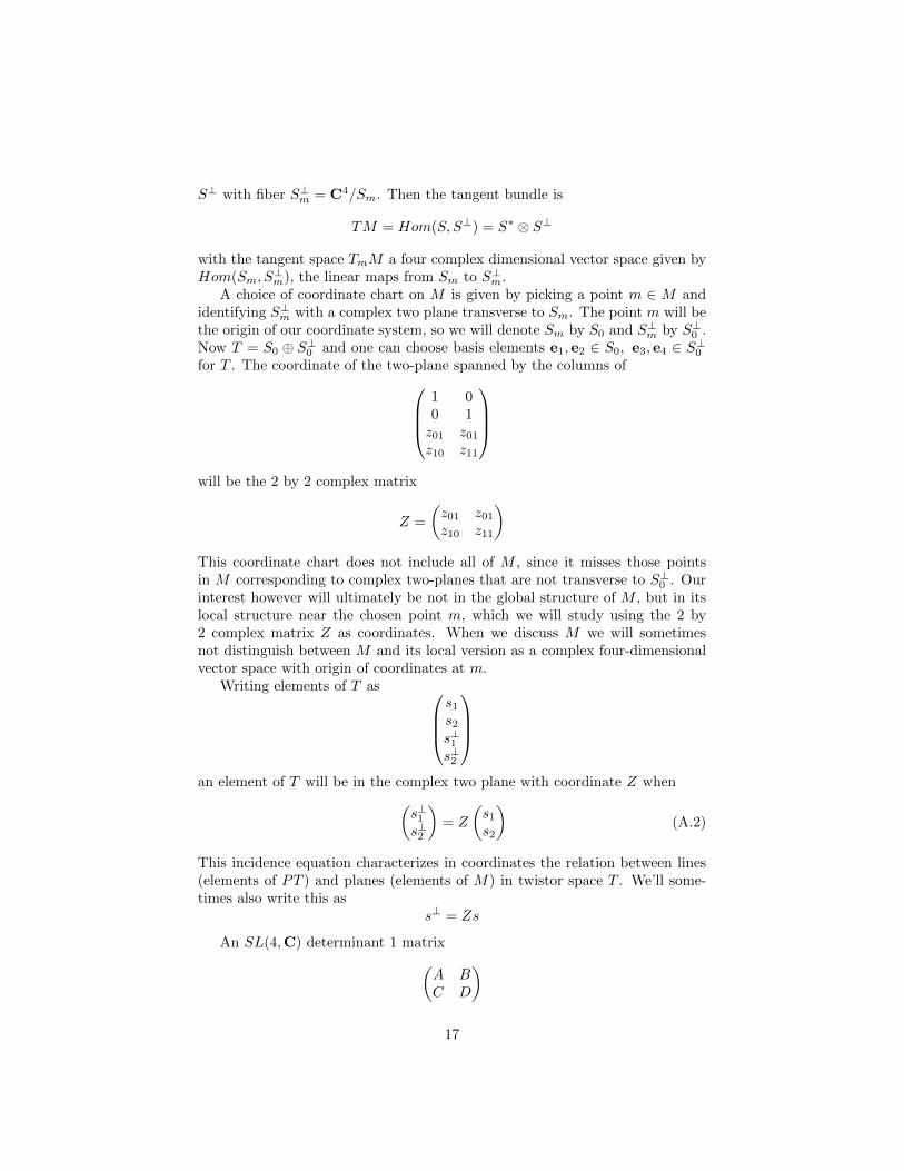
A choice of coordinate chart on M is given by picking a point m ∈ M andidentifying S⊥m with a complex two plane transverse to Sm. The point m will bethe origin of our coordinate system, so we will denote Sm by S0 and S⊥m by S⊥0 .Now T = S0 ⊕ S⊥0 and one can choose basis elements e1, e2 ∈ S0, e3, e4 ∈ S⊥0for T . The coordinate of the two-plane spanned by the columns of

1 00 1z01 z01z10 z11

will be the 2 by 2 complex matrix

Z =

(z01 z01z10 z11

)This coordinate chart does not include all of M , since it misses those pointsin M corresponding to complex two-planes that are not transverse to S⊥0 . Ourinterest however will ultimately be not in the global structure of M , but in itslocal structure near the chosen point m, which we will study using the 2 by2 complex matrix Z as coordinates. When we discuss M we will sometimesnot distinguish between M and its local version as a complex four-dimensionalvector space with origin of coordinates at m.

Writing elements of T as s1s2s⊥1s⊥2

an element of T will be in the complex two plane with coordinate Z when(

s⊥1s⊥2

)= Z

(s1s2

)(A.2)

This incidence equation characterizes in coordinates the relation between lines(elements of PT ) and planes (elements of M) in twistor space T . We’ll some-times also write this as

s⊥ = Zs

An SL(4,C) determinant 1 matrix(A BC D

)

17

acts on T by (ss⊥

)→(As+Bs⊥

Cs+Ds⊥

)On lines in the plane Z this is[

sZs

]→[As+BZsCs+DZs

]=

[(A+BZ)s

(C +DZ)(A+BZ)−1(A+BZ)s

]so the corresponding action on M will be given by

Z → (C +DZ)(A+BZ)−1

Since Λ2(S0) = Λ2(S⊥0 ) = C, S0 and S⊥0 have (up to scalars) unique choicesεS0 and εS⊥

0of non-degenerate antisymmetric bilinear forms, and corresponding

choices of SL(2,C) ⊂ GL(2,C) acting on S0 and S⊥0 . These give (again, up toscalars), a unique choice of a non-degenerate symmetric form on Hom(S0, S

⊥0 ),

such that〈Z,Z〉 = detZ

The subgroup

Spin(4,C) = SL(2,C)× SL(2,C) ⊂ SL(4,C)

of matrices of the form (A 00 D

)with

detA = detD = 1

acts on M in coordinates by

Z → DZA−1

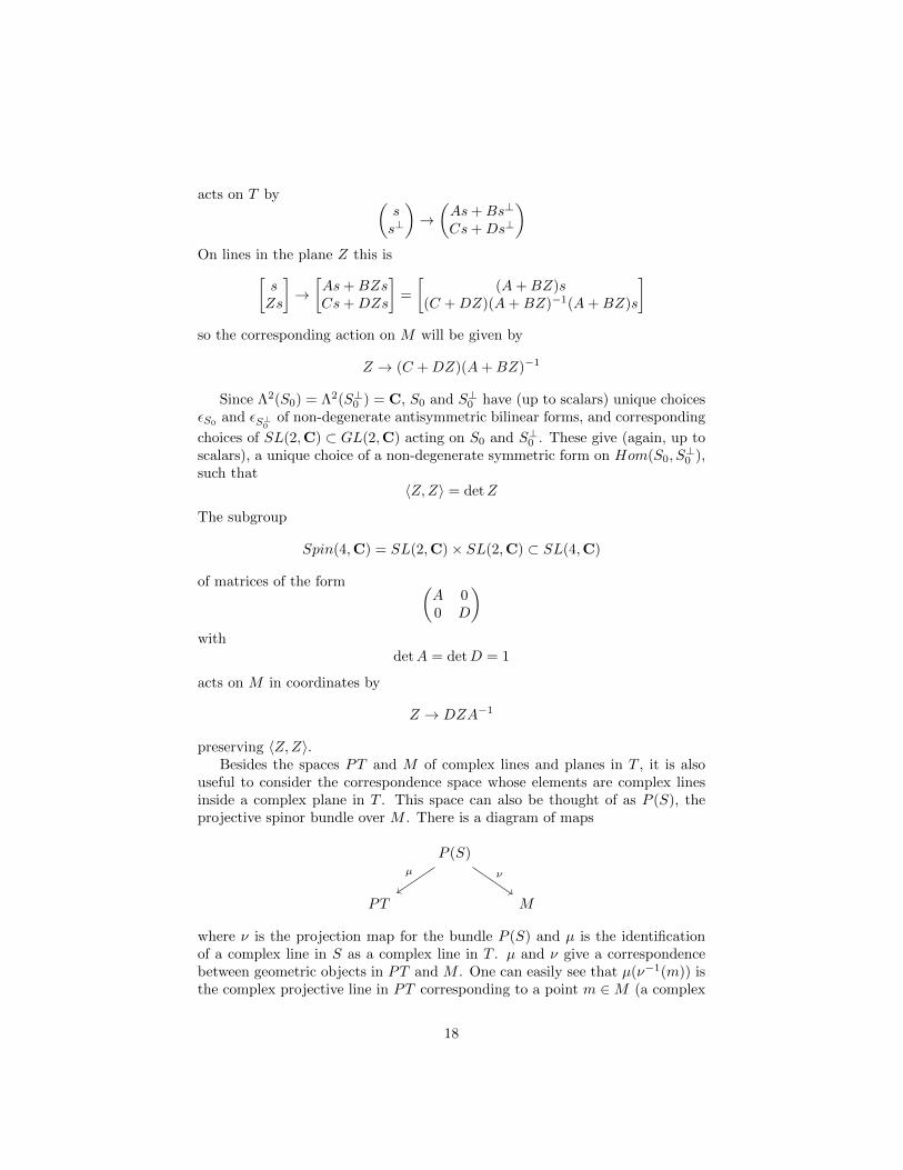
preserving 〈Z,Z〉.Besides the spaces PT and M of complex lines and planes in T , it is also

useful to consider the correspondence space whose elements are complex linesinside a complex plane in T . This space can also be thought of as P (S), theprojective spinor bundle over M . There is a diagram of maps

P (S)

PT M

µ ν

where ν is the projection map for the bundle P (S) and µ is the identificationof a complex line in S as a complex line in T . µ and ν give a correspondencebetween geometric objects in PT and M . One can easily see that µ(ν−1(m)) isthe complex projective line in PT corresponding to a point m ∈M (a complex

18

two plane in T is a complex projective line in PT ). In the other direction,ν(µ−1) takes a point p in PT to α(p), a copy of CP 2 in M , called the “α-plane”corresponding to p.

In our chosen coordinate chart, this diagram of maps is given by

(Z, s) ∈ P (S)

[sZs

]∈ PT Z ∈M

µν

The incidence equation A.2 relating PT and M implies that an α-plane is a nullplane in the metric discussed above. Given two points Z1, Z2 inM correspondingto the same point in PT , their difference satisfies

s⊥ = (Z1 − Z2)s = 0

Z1 − Z2 is not an invertible matrix, so has determinant 0 and is a null vector.

A.2 The Penrose-Ward transform

The Penrose transform relates solutions of conformally-invariant wave equationson M to sheaf cohomology groups, identifying

• Solutions to a helicity k2 holomorphic massless wave equation on U .

• The sheaf cohomology group

H1(U ,O(−k − 2))

Here U ⊂M and U ⊂ PT are open sets related by the twistor correspondence,i.e.

U = µ(ν−1(U))

We will be interested in cases where U and U are orbits in M and PT for areal form of SL(4,C). Here O(−k − 2) is the sheaf of holomorphic sections ofthe line bundle L⊗(−k−2) where L is the tautological line bundle over PT . Fora detailed discussion, see for instance chapter 7 of [35].

The Penrose-Ward transform is a generalization of the above, introducinga coupling to gauge fields. One aspect of this is the Ward correspondence, anisomorphism between

• Holomorphic anti-self-dual GL(n,C) connections A on U ⊂M .

• Holomorphic rank n vector bundles E over U ⊂ PT .

19

Here “anti-self-dual” means the curvature of the connection satisfies

∗FA = −FA

where ∗ is the Hodge dual. There are some restrictions on the open set U , andE needs to be trivial on the complex projective lines corresponding to pointsm ∈ U .

In one direction, the above isomorphism is due to the fact that the curva-ture FA is anti-self-dual exactly when the connection A is integrable on theintersection of an α-plane with U . One can then construct the fiber Ep of Eat p as the covariantly constant sections of the bundle with connection on thecorresponding α-plane in M . In the other direction, one can construct a vectorbundle E on U by taking as fiber at m ∈ U the holomorphic sections of Eon the corresponding complex projective line in PT . Parallel transport in thisvector bundle can be defined using the fact that two points m1,m2 in U on thesame α-plane correspond to intersecting projective lines in PT . For details, seechapter 8 of [35] and chapter 10 of [28].

Given an anti-self-dual gauge field as above, the Penrose transform can begeneralized to a Penrose-Ward transform, relating

• Solutions to a helicity k holomorphic massless wave equation on U , coupledto a vector bundle E with anti-self-dual connection A.

• The sheaf cohomology group

H1(U ,O(E)(−k − 2))

For more about this generalization, see [16].

A.3 Twistor geometry and real forms

So far we have only considered complex twistor geometry, in which the relationto space-time geometry is that M is a complexified version of a four real dimen-sional space-time. From the point of view of group symmetry, the Lie algebraof SL(4,C) is the complexification

sl(4,C) = g⊗C

for several different real Lie algebras g, which are the real forms of sl(4,C).To organize the possibilities, recall that SL(4,C) is Spin(6,C), the spin groupfor orthogonal linear transformations in six complex dimensions, so sl(4,C) =so(6,C). If one instead considers orthogonal linear transformations in six realdimensions, there are different possible signatures of the inner product to con-sider, all of which become equivalent after complexification. This correspondsto the possible real forms

g = so(3, 3), so(4, 2), so(5, 1), and so(6)

which we will discuss (there’s another real form, su(3, 1), which we won’t con-sider). For more about real methods in twistor theory, see [42].

20

A.3.1 Spin(3, 3) = SL(4,R)

The simplest way to get a real version of twistor geometry is to take the discus-sion of section A and replace complex numbers by real numbers. Equivalently,one can look at subspaces invariant under the usual conjugation, given by themap σ

σ

s1s2s⊥1s⊥2

=

s1s2s⊥1s⊥2

which acts not just on T but on PT and M . The fixed point set of the actionon M is M2,2 = G2,4(R), the Grassmanian of real two-planes in R4. As amanifold, G2,4(R) is S2 × S2, quotiented by a Z2. M2,2 is acted on by thegroup Spin(3, 3) = SL(4,R) of conformal transformations. σ acting on PTacts on the CP 1 corresponding to a point in M2,2 with an action whose fixedpoints form an equatorial circle.

Coordinates can be chosen as in the complex case, but with everything real.A point in M2,2 is given by a real 2 by 2 matrix, which can be written in theform

Z =

(x0 + x3 x1 − x2x1 + x2 x0 − x3

)for real numbers x0, x1, x2, x3. M2,2 is acted on by the group Spin(3, 3) =SL(4,R) of conformal transformations as in the complex case by

Z → (C +DZ)(A+BZ)−1

with the subgroup of rotations

Z → DZA−1

for A,D ∈ SL(2,R) given by

Spin(2, 2) = SL(2,R)× SL(2,R)

This subgroup preserves

〈Z,Z〉 = detZ = x20 − x23 − x21 + x22

For the Penrose transform in this case, see Atiyah’s account in section 6.5of [7]. For the Ward correspondence, see section 10.5 of [28].

A.3.2 Spin(4, 2) = SU(2, 2)

The real case of twistor geometry most often studied (a good reference is [35]) isthat where the real space-time is the physical Minkowski space of special relativ-ity. The conformal compactification of Minkowski space is a real submanifold ofM , denoted here by M3,1. It is acted upon transitively by the conformal group

21

Spin(4, 2) = SU(2, 2). This conformal group action on M3,1 is most naturallyunderstood using twistor space, as the action on complex planes in T comingfrom the action of the real form SU(2, 2) ⊂ SL(4,C) on T .

SU(2, 2) is the subgroup of SL(4,C) preserving a real Hermitian form Φ ofsignature (2, 2) on T = C4. In our coordinates for T , a standard choice for Φ isgiven by

Φ

((ss⊥

),

(s′

(s⊥)′

))=(s s⊥

)(0 11 0

)(s′

(s⊥)′

)= s†(s⊥)′ + (s⊥)†s′ (A.3)

Minkowski space is given by complex planes on which Φ = 0, so

Φ

((sZs

),

(sZs

))= s†(Z + Z†)s = 0

Thus coordinates of points on Minkowski space are anti-Hermitian matrices Z,which can be written in the form

Z = −i(x0 + x3 x1 − ix2x1 + ix2 x0 − x3

)= −i(x01 + x · σ)

where σj are the Pauli matrices. The metric is the usual Minkowski metric,since

〈Z,Z〉 = detZ = −x20 + x21 + x22 + x23

One can identify compactified Minkowski space M3,1 as a manifold with the Liegroup U(2) which is diffeomorphic to (S3 × S1)/Z2. The identification of thetangent space with anti-Hermitian matrices reflects the usual identification ofthe tangent space of U(2) at the identity with the Lie algebra of anti-Hermitianmatrices.

SL(4,C) matrices are in SU(2, 2) when they satisfy(A† C†

B† D†

)(0 11 0

)(A BC D

)=

(0 11 0

)The Poincare subgroup P of SU(2, 2) is given by elements of SU(2, 2) of theform (

A 0C (A†)−1

)where A ∈ SL(2,C) and A†C = −C†A. These act on Minkowski space by

Z → (C + (A†)−1Z)A−1 = (A†)−1ZA−1 + CA−1

One can show that CA−1 is anti-Hermitian and gives arbitrary translations onMinkowski space. The Lorentz subroup is Spin(3, 1) = SL(2,C) acting by

Z → (A†)−1ZA−1

Here SL(2,C) is acting by the standard representation on S0, and by theconjugate-dual representation on S⊥0 .

22

Note that, for the action of the Lorentz SL(2,C) subgroup, twistors writtenas elements of S0⊕S⊥0 behave like usual Dirac spinors (direct sums of a standardSL(2,C) spinor and one in the conjugate-dual representation), with the usualDirac adjoint, in which the SL(2,C)-invariant inner product is given by thesignature (2, 2) Hermitian form

〈ψ1, ψ2〉 = ψ†1γ0ψ2

Twistors, with their SU(2, 2) conformal group action and incidence relation tospace-time points, are however something different than Dirac spinors.

The SU(2, 2) action on M has six orbits: M++,M−−,M+0,M−0,M00, wherethe subscript indicates the signature of Φ restricted to planes correspondingto points in the orbit. The last of these is a closed orbit M3,1, compactifiedMinkowski space. Acting on projective twistor space PT , there are three orbits:PT+, PT−, PT0, where the subscript indicates the sign of Φ restricted to theline in T corresponding to a point in the orbit. The first two are open orbitswith six real dimensions, the last a closed orbit with five real dimensions. Thepoints in compactified Minkowski space M00 = M3,1 correspond to projectivelines in PT that lie in the five dimensional space PT0. Points in M++ and M−−correspond to projective lines in PT+ or PT− respectively.

One can construct infinite dimensional irreducible unitary representations ofSU(2, 2) using holomorphic geometry on PT+ or M++, with the Penrose trans-form relating the two constructions [15]. For PT+ the closure of the orbit PT+,the Penrose transform identifies the sheaf cohomology groups H1(PT+,O(−k−2)) for k > 0 with holomorphic solutions to the helicity k

2 wave equation onM++. Taking boundary values on M3,1, these will be real-analytic solutions tothe helicity k

2 wave equation on compactified Minkowski space. If one insteadconsiders the sheaf cohomology H1(PT+,O(−k − 2)) for the open orbit PT+and takes boundary values on M3,1 of solutions on M++, the solutions will behyperfunctions, see [36].

The Ward correspondence relates holomorphic vector bundles on PT+ withanti-self-dual GL(n,C) gauge fields on M++. However, in this Minkowski sig-nature case, all solutions to the anti-self-duality equations as boundary valuesof such gauge fields are complex, so one does not get anti-self-dual gauge fieldsfor compact gauge groups like SU(n).

A.3.3 Spin(5, 1) = SL(2,H)

Changing from Minkowski space-time signature (3, 1) to Euclidean space-timesignature (4, 0), the compactified space-time M4 = S4 is again a real subman-ifold of M . To understand the conformal group and how twistors work in thiscase, it is best to work with quaternions instead of complex numbers, iden-tifying T = H2. When working with quaternions, one can often instead usecorresponding complex 2 by 2 matrices, with a standard choice

q = q0 + q1i + q2j + q3k↔ q0 − i(q1σ1 + q2σ2 + q3σ3)

23

For more details of the quaternionic geometry that appears here, see [7] or [34]The relevant conformal group acting on S4 is Spin(5, 1) = SL(2,H), again

best understood in terms of twistors and the linear action of SL(2,H) on T =H2. The group SL(2,H) is the group of quaternionic 2 by 2 matrices satisfying asingle condition that one can think of as setting the determinant to one, althoughthe usual determinant does not make sense in the quaternionic case. Here onecan interpret the determinant using the isomorphism with complex matrices,or, at the Lie algebra level, sl(2,H) is the Lie algebra of 2 by 2 quaternionicmatrices with purely imaginary trace.

While one can continue to think of points in S4 ⊂M as complex two planes,one can also identify these complex two planes as quaternionic lines and S4 asHP1, the projective space of quaternionic lines in H2. The conventional choiceof identification between C2 and H is

s =

(s1s2

)↔ s = s1 + s2j

One can then think of the quaternionic structure as providing an alternatenotion of conjugation than the usual one, given instead by left multiplying byj ∈ H. Using jzj = −z one can show that

σ

s1s2s⊥1s⊥2

=

−s2s1−s⊥2s⊥1

(A.4)

σ satisfies σ2 = −1 on T , so σ2 = 1 on PT . We will see later that while σ hasno fixed points on PT , it does fix complex projective lines.

The same coordinates used in the complex case can be used here, where nowS⊥0 is a quaternionic line transverse to S0, so coordinates on T are the pair ofquaternions (

ss⊥

)These are also homogeneous coordinates for points on S4 = HP1 and our choiceof Z ∈ H given by (

sZs

)as the coordinate in a coordinate system with origin the point with homogeneouscoordinates (

10

)The point at ∞ will be the one with homogeneous coordinates(

01

)

24

This is the quaternionic version of the usual sort of choice of coordinates in thecase of S2 = CP 1, replacing complex numbers by quaternions. The coordinateof a point on S4 with homogeneous coordinates(

ss⊥

)will be

s⊥s−1 =(s⊥1 + s⊥2 j)(s1 − s1j)|s1|2 + |s2|2

=s⊥1 s1 + s⊥2 s2 + (−s⊥1 s2 + s⊥2 s1)j

|s1|2 + |s2|2(A.5)

A coordinate of a point will now be a quaternion Z = x0 + x1i + x2j + x3kcorresponding to the 2 by 2 complex matrix

Z = x01− ix · σ =

(x0 − ix3 −ix1 − x2−ix1 + x2 x0 + ix3

)The metric is the usual Euclidean metric, since

〈Z,Z〉 = detZ = x20 + x21 + x22 + x23

The conformal group SL(2,H) acts on T = H2 by the matrix(A BC D

)where A,B,C,D are now quaternions, satisfying together the determinant 1condition. These act on the coordinate Z as in the complex case, by

Z → (C +DZ)(A+BZ)−1

The Euclidean group in four dimensions will be the subgroup of elements of theform (

A 0C D

)such that A and D are independent unit quaternions, thus in the group Sp(1) =SU(2), and C is an arbitrary quaternion. The Euclidean group acts by

Z → DZA−1 + CA−1

with the spin double cover of the rotational subgroup now Spin(4) = Sp(1) ×Sp(1). Note that spinors behave quite differently than in Minkowski space:there are independent unitary SU(2) actions on S0 and S⊥0 rather than a non-unitary SL(2,C) action on S0 that acts at the same time on S⊥0 by the conjugatetranspose representation.

The projective twistor space PT is fibered over S4 by complex projectivelines

CP 1 PT = CP 3

S4 = HP 1

π (A.6)

25

The projection map π is just the map that takes a complex line in T identifiedwith H2 to the corresponding quaternionic line it generates (multiplying ele-ments by arbitrary quaternions). In this case the conjugation map σ of A.4 hasno fixed points on PT , but does fix the complex projective line fibers and thusthe points in S4 ⊂M . The action of σ on a fiber takes a point on the sphere tothe opposite point, so has no fixed points.

Note that the Euclidean case of twistor geometry is quite different and muchsimpler than the Minkowski one. The correspondence space P (S) (here thecomplex lines in the quaternionic line specifying a point in M4 = S4) is just PTitself, and the twistor correspondence between PT and S4 is just the projectionπ. Unlike the Minkowski case where the real form SU(2, 2) has a non-trivialorbit structure when acting on PT , in the Euclidean case the action of the realform SL(2,H) is transitive on PT .

In the Euclidean case, the projective twistor space has another interpreta-tion, as the bundle of orientation preserving orthogonal complex structures onS4. A complex structure on a real vector space V is a linear map J such thatJ2 = −1, providing a way to give V the structure of a complex vector space(multiplication by i is multiplication by J). J is orthogonal if it preserves aninner product on V . While on R2 there is just one orientation-preserving or-thogonal complex structure, on R4 the possibilities can be parametrized by asphere S2. The fiber S2 = CP 1 of A.6 above a point on S4 can be interpretedas the space of orientation preserving orthogonal complex structures on the fourreal dimensional tangent space to S4 at that point.

One way of exhibiting these complex structures on R4 is to identify R4 = Hand then note that, for any real numbers x1, x2, x3 such that x21 + x22 + x23 = 1,one gets an orthogonal complex structure on R4 by taking

J = x1i + x2j + x3k

Another way to see this is to note that the rotation group SO(4) acts on orthogo-nal complex structures, with a U(2) subgroup preserving the complex structure,so the space of these is SO(4)/U(2), which can be identified with S2.

More explicitly, in our choice of coordinates, the projection map is

π :

[s

s⊥ = Zs

]→ Z =

(x0 − ix3 −ix1 − x2−ix1 + x2 x0 + ix3

)For any choice of s in the fiber above Z, s⊥ associates to the four real coordinatesspecifying Z an element of C2. For instance, if s =

(1, 0), the identification of

R4 with C2 is x0x1x2x3

↔ (x0 − ix3−ix1 + x2

)

The complex structure on R4 one gets is not changed if s gets multiplied by acomplex scalar, so it just depends on the point [s] in the CP 1 fiber.

26

For another point of view on this, one can see that for each point p ∈ PT ,the corresponding α-plane ν(µ−1(p)) in M intersects its conjugate σ(ν(µ−1(p)))in exactly one real point, π(p) ∈ M4. The corresponding line in PT is the linedetermined by the two points p and σ(p). At the same time, this α-planeprovides an identification of the tangent space to M4 at π(p) with a complextwo plane, the α-plane itself. The CP 1 of α -planes corresponding to a point inS4 are the different possible ways of identifying the tangent space at that pointwith a complex vector space. The situation in the Minkowski space case is quitedifferent: there if CP 1 ⊂ PT0 corresponds to a point Z ∈ M3,1, each point pin that CP 1 gives an α-plane intersecting M3,1 in a null line, and the CP 1 canbe identified with the “celestial sphere” of null lines through Z.

In the Euclidean case , the Penrose transform will identify the sheaf cohomol-ogy group H1(π−1(U),O(−k − 2)) for k > 0 with solutions of helicity k

2 linearfield equations on an open set U ⊂ S4. Unlike in the Minkowski space case, inEuclidean space there are U(n) bundles E with connections having non-trivialanti-self-dual curvature. The Ward correspondence between such connectionsand holomorphic bundles E on PT for U = S4 has been the object of inten-sive study, see for example Atiyah’s survey [7]. The Penrose-Ward transformidentifies

• Solutions to a field equation on U for sections Γ(Sk ⊗ E), with covariantderivative given by an anti-self-dual connection A, where Sk is the k’thsymmetric power of the spinor bundle.

• The sheaf cohomology group

H1(U ,O(E)(−k − 2))

where U = π−1U .

For the details of the Penrose-Ward transform in this case, see [21].

A.3.4 Spin(6) = SU(4)

If one picks a positive definite Hermitian inner product on T , this determines asubgroup SU(4) = Spin(6) that acts on T , and thus on PT,M and P (S). Onehas

PT =SU(4)

U(3), M =

SU(4)

S(U(2)× U(2)), P (S) =

SU(4)

S(U(1)× U(2))

and the SU(4) action is transitive on these three spaces. There is no four realdimensional orbit in M that could be interpreted as a real space-time that wouldgive M after complexification.

In this case the Borel-Weil-Bott theorem relates sheaf-cohomology groupsof equivariant holomorphic vector-bundles on PT,M and P (S), giving themexplicitly as certain finite dimensional irreducible representations of SU(4). Formore details of the relation between the Penrose transform and Borel-Weil-Bott, see [8]. The Borel-Weil-Bott theorem [10] can be recast in terms of index

27

theory, replacing the use of sheaf-cohomology with the Dirac equation [11]. Fora more general discussion of the relation of representation theory and the Diracoperator, see [22].

B Euclidean quantum fields

But besides this, by freeingourselves from the limitation ofthe Lorentz group, which hasproduced all the well-knowndifficulties of quantum fieldtheory, one has here a possibility— if this is indeed necessary — ofproducing new theories. That is,one has the possibility ofconstructing new theories in theEuclidean space and thentranslating them back into theLorentz system to see what theyimply.

J. Schwinger, 1958[47]

Should the Feynman pathintegral be well-defined only inEuclidean space, as axiomaticianswould have it, then there seemsto exist a very real problem whendealing with Weyl fields as in thetheory of weak interactions or inits unification with QCD.

P. Ramond, 1981[60]

A certain sense of mysterysurrounds Euclidean fermions.

A. Jaffe and G. Ritter, 2008[75]

That one chirality of Euclidean space-time rotations appears after analyticcontinuation to Minkowski space-time as an internal symmetry is the most hardto believe aspect of the proposed framework for a unified theory outlined inthis paper. One reason for the very long time that has passed since an earlierembryonic version of this idea (see [39]) is that the author has always foundthis hard to believe himself. While the fact that the quantization of Euclidean

28

spinor fields is not straightforward is well-known, Schwinger’s early hope thatthis might have important physical significance (see above) does not appear tohave attracted much attention. In this section we’ll outline the basic issue withEuclidean spinor fields, and argue that common assumptions about analyticcontinuation of the space-time symmetry do not hold in this case. This issuebecomes apparent in the simplest possible context of free field theory. There arealso well-known problems when one attempts to construct a non-perturbativelattice-regularized theory of chiral spinors coupled to gauge fields.

Since Schwinger’s first proposal in 1958[46], over the years it has becomeincreasingly clear that the quantum field theories governing our best under-standing of fundamental physics have a much simpler behavior if one takes timeto be a complex variable, and considers the analytic continuation of the theoryto imaginary values of the time parameter. In imaginary time the invariant no-tion of distance between different points becomes positive, path integrals oftenbecome well-defined rather than formal integrals, field operators commute, andexpectation values of field operators are conventional functions rather than theboundary values of holomorphic functions found at real time.

While momentum eigenvalues can be arbitrarily positive or negative, energyeigenvalues go in one direction only, which by convention is that of positive ener-gies. Having states supported only at non-negative energies implies (by Fouriertransformation) that, as a function of complex time, states can be analyticallycontinued in one complex half plane, not the other. A quantum theory in Eu-clidean space has a fundamental asymmetry in the direction of imaginary time,corresponding to the fundamental asymmetry in energy eigenvalues.

Quantum field theories can be characterized by their n-point Wightman(Minkowski space-time) or Schwinger (Euclidean space-time) functions, withthe Wightman functions not actual functions, but boundary values of analyticcontinuations of the Schwinger functions. For free field theories these are alldetermined by the 2-point functions W2 or S2. The Wightman function W2 isPoincare-covariant, while the Schwinger function S2 is Euclidean-covariant.

This simple relation between the Minkowski and Euclidean space-time freefield theories masks a much more subtle relationship at the level of fields, statesand group actions on these. In both cases one can construct fields and aFock space built out of a single-particle state space carrying a representationof the space-time symmetry group. For the Minkowski theory, fields are non-commuting operators obeying an equation of motion and the single-particle statespace is an irreducible unitary representation of the Poincare group.

The Euclidean theory is quite different. Euclidean fields commute and donot obey an equation of motion. The Euclidean single-particle state space isa unitary representation of the Euclidean group, but far from irreducible. Itdescribes not physical states, but instead all possible trajectories in the spaceof physical states (parametrized by imaginary time). The Euclidean state spaceand the Euclidean fields are not in any sense analytic continuations of the cor-responding Minkowski space constructions. For a general theory encompassingthe relation between the Euclidean group and Poincare group representations,see [64].

29

One can recover the physical Minkowski theory from the Euclidean theory,but to do so one must break the Euclidean symmetry by choosing an imaginarytime direction. In the following sections we will outline the relation between theMinkowski and Euclidean theories for the cases of the harmonic oscillator, thefree scalar field theory, and the free chiral spinor field theory.

B.1 The harmonic oscillator

The two-point Schwinger function for the one-dimensional quantum harmonicoscillator of frequency ω (ω > 0) is

S2(τ) =1

(2π)(2ω)e−ω|τ |

with Fourier transform

S2(s) =1√2π

∫ ∞−∞

eisτS2(τ)dτ =1

(2π)3/21

s2 + ω2

In the complex z = t+ iτ plane, S2 can be analytically continued to the upperhalf plane as

1

(2π)(2ω)eiωz

and to the lower half plane as

1

(2π)(2ω)e−iωz

The Wightman functions are the analytic continuations to the t (real z) axis,so come in two varieties:

W−2 (t) = limε→0+

1

(2π)(2ω)eiω(t+iε)

and

W+2 (t) = lim

ε→0+

1

(2π)(2ω)e−iω(t−iε)

The conventional interpretation of W±2 is not as functions, but as distribu-tions, given as the boundary values of holomorphic functions. Alternatively (seeappendix C), one can interpret W±2 (t) as the lower and upper half-plane holo-morphic functions defining a hyperfunction. Like distributions, hyperfunctionscan be thought of a elements of a dual space to a space of well-behaved testfunctions, in this case a space of real analytic functions. The Fourier transformof W2 is then the hyperfunction

W2(E) =i

(2π)3/21

ω2 − E2

30

which is a sum of terms W±2 (E) supported at ω > 0 and −ω < 0. Note thatthe convention that e−iEt has positive energy means that Fourier transforms ofpositive energy functions are holomorphic for τ < 0.

The physical state space of the harmonic oscillator is determined by thesingle-particle state space H1 = C. H1 is the state space for a single quantum,it can be thought of as the space of positive energy solutions to the equation ofmotion

(d2

dt2+ ω2)φ = 0 (B.1)

H1 can also be constructed using W+2 , by defining

(f, g) =

∫ ∞−∞

∫ ∞−∞

f(t2)W+2 (t2 − t1)g(t1)dt1dt2

=

∫ ∞−∞

∫ ∞−∞

f(t2)e−iω(t2−t1)

(2π)(2ω)g(t1)dt1dt2

=1

2ωf(ω)g(ω)

for f, g functions in S(R) and taking the space of equivalence classes

H1 = [f ] ∈ f ∈ S(R)/(f, f) = 0

One can identify such equivalence classes as

[f ] =1√2ωf(ω)

H1 is C with standard Hermitian inner product

〈[f ], [g]〉 =1

2ωf(ω)g(ω)

Note that it doesn’t matter whether one takes real or complex valued functionsf , in either case one gets the same quotient complex vector space H1.

Given H1 and the inner product 〈·, ·〉, the full state space H is an innerproduct space given by the Fock space construction, with

H = S∗(H1) =

∞⊕k=0

Sk(H1)

In this case the symmetrized tensor product Sk(H1) of k copies of H1 = C isjust again C, the states with k-quanta. A creation operator a†(f) (for f real)acts by symmetrized tensor product with [f ] and a(f) is the adjoint operator.One can define an operator

φ(f) = a(f) + a†(f)

and then〈0|φ(f)φ(g)|0〉 = 〈[f ], [g]〉

31

φ(t) should be interpreted as an operator-valued distribution, writing

φ(f) =

∫ ∞−∞

φ(t)f(t)dt

φ satisfies the equation of motion B.1.One can use the Schwinger function S2 to set up a Euclidean (imaginary

time τ) Fock space, taking E1 to be the space of real-valued functions in S(R)with inner product

(f, g)E1 =

∫ ∞−∞

∫ ∞−∞

f(τ2)S2(τ2 − τ1)g(τ1)dτ1dτ2

=

∫ ∞−∞

∫ ∞−∞

f(τ2)e−ω|τ2−τ1|

(2π)(2ω)g(τ1)dτ1dτ2

The Fock space will beE = S∗(E1 ⊗C)

based on the complexification of E1, with operators a†E(f), aE(f), φE(f), φE(τ)

defined for f ∈ E1. Expectation values of products of fields φE(f) for suchreal-valued f can be given a probabilistic interpretation (see for instance [19]).

Note that the imaginary time state space and operators are of a quite dif-ferent nature than those for real time. The operators φE(τ) do not satisfy anequation of motion, and commute for all τ . They describe not the annihila-tion and creation of a single quantum, but an arbitrary path in imaginary timeof a configuration-space observable. The state space is much larger than thereal-time state space, with E1 infinite dimensional as opposed to H1 = C.

One way to reconstruct the physical real-time theory from the Euclideantheory is to consider the fixed τ subspace of E1⊗C of complex functions localizedat τ0. Here f(τ) = aδ(τ − τ0) for a ∈ C and one defines a Hermitian innerproduct on E1 ⊗C by

(f, g)E1⊗C =

∫ ∞−∞

∫ ∞−∞

f(τ2)S2(τ2 − τ1)g(τ1)dτ1dτ2

While elements of E1 satisfy no differential equation and have no dynamics,one does have an action of time translations on E1, with translation by τ0 takingaδ(τ) to aδ(τ − τ0). Since the inner product satisfies

(aδ(τ), bδ(τ − τ0)) = abe−ω|τ0|

one sees that one can define a Hamiltonian operator generating imaginary timetranslations on these states by taking H to be multiplication by ω. The imagi-nary time translation operator e−τ0ω can be analytically continued from τ0 > 0to real time t as

U(t) = e−itω

32

Another way to reconstruct the real-time theory is the Osterwalder-Schradermethod, which begins by picking out the subspace E+1 ⊂ E1 ⊗ C of functionssupported on τ < 0. Defining a time reflection operator on E1 by

Θf(τ) = f(−τ)

one can define(f, g)OS = (Θf, g)E1⊗C

The physical H1 can then be recovered as

H1 =f ∈ E+1

(f, f)OS = 0

Note that for f, g ∈ E+1 one has (since f, g are supported for τ < 0)

(f, g)OS =

∫ ∞−∞

∫ ∞−∞

f(−τ2)e−ω|τ2−τ1|

(2π)(2ω)g(τ1)dτ1dτ2

=

∫ ∞−∞

∫ ∞−∞

f(τ2)eω(τ2+τ1)

(2π)(2ω)g(τ1)dτ1dτ2

=1

(2π)(2ω)

∫ ∞−∞

f(τ2)eωτ2dτ2

∫ ∞−∞

g(τ1)eωτ1dτ1

=1

2ωf(−iω)g(−iω)

This gives a mapf ∈ E+1 → [f ] ∈ H1

similar to that of the real-time case

f → [f ] =1√2ωf(−iω) =

1√2ω√

2π

∫ ∞−∞

eωτf(τ)dτ

B.2 Relativistic scalar fields

The theory of a mass m free real scalar field in 3 + 1 dimensions can be treatedas a straightforward generalization of the above discussion of the harmonic oscil-lator, treating time in the same way, spatial dimensions with the usual Fouriertransform. Defining

ωp =√|p|2 +m2

the Fourier transform of the Schwinger function is

S2(s,p) =1

(2π)31

s2 + ω2p

and the Schwinger function itself is

S2(τ,x) =1

(2π)2

∫R4

ei(τs+x·p) 1

(2π)31

s2 + ω2p

dsd3p

=m

(2π)3√τ2 + |x|2

K1(m√τ2 + |x|2)

33

where K1 is a modified Bessel function. This has an analytic continuation tothe z = t+ iτ plane, with branch cuts on the t axis from |x| to ∞ and −|x| to−∞.

−|x| |x|t

τ

The Wightman function W+2 (t,x) will be defined as the limit of the analytic

continuation of S2 as one approaches the t-axis from negative values of τ . Thiswill be analytic for spacelike t < |x|, but will approach a branch cut for timeliket > |x|. The Fourier transform of W±2 will be, as a hyperfunction (in thetime-energy coordinate)

W2(p) =1

(2π)3i

ω2p − E2

or, as a distribution, the delta-function distribution

W+2 (p) =

1

(2π)2θ(E)δ(E2 − ω2

p)

on the positive energy mass shell E = +ωp. Here W+2 (x) is

W+2 (t,x) =

1

(2π)4

∫R3

1

2ωpe−iωpteip·xd3p

As in the harmonic oscillator case, one can use it to reconstruct the singleparticle state space H1, defining

(f, g) =

∫R4

∫R4

f(x)W+2 (x− y)g(y)d4xd4y

for f, g ∈ S(R4) (R4 is Minkowski space), and equivalence classes

H1 = [f ] ∈ f ∈ S(R4)/(f, f) = 0

The inner product on H1 is given by

〈[f ], [g]〉 =

∫R4

θ(E)δ(E2 − ω2p)f(p)g(p)d4p

34

where p = (E,p) and θ is the Heaviside step function. Elements [f ] of H1 can

be represented by functions f on R3 of the form

f(p) = f(ωp,p)

In this representation, H1 has the Lorentz-invariant Hermitian inner product

〈[f ], [g]〉 =

∫R3

f(p)g(p)d3p

2ωp

Using the Fock space construction (as in the harmonic oscillator case, whereH1 = C), the full physical state space is

H = S∗(H1) =∞⊕k=0

Sk(H1)

with creation operators a†(f) acting by symmetrized tensor product with [f ].a(f) is the adjoint operator and one can define field operators by

φ(f) = a(f) + a†(f)

Writing these distributions as φ(t,x), one recovers the usual description ofWightman functions as

W+2 (x− y) = 〈0|φ(x)φ(y)|0〉

The operators φ(x) satisfy the equation of motion(∂2

∂t2−∆ +m2

)φ = 0

and φ(x), φ(y) commute for x and y space-like separated, but not for time-likeseparations (due to the branch cuts described above).

The Euclidean (imaginary time) theory has the Fock space

E = S∗(E1 ⊗C)

where E1 is the space of real-valued functions in S(R4) (now R4 is Euclideanspace) with inner product

(f, g)E1 =

∫R4

∫R4

f(x)S2(x− y)g(y)d4xd4y

This Fock space comes with operators a†E(f), aE(f), φE(f), φE(x) defined for

f ∈ E1. Expectation values of products of fields φ(f) for such real-valued f canbe given a probabilistic interpretation in terms of a Gaussian measure on thedistribution space S ′(R4) (for details, see [19]).

35

As in the harmonic oscillator case, there are two ways to recover the realtime theory from the Euclidean theory. In the first, one takes H1 ⊂ E1 to be thefunctions on Euclidean space-time localized at a specific value of τ , say τ = 0,of the form

f(τ,x) =1

2πδ(τ)F (x)

Evaluating the inner product for these, one finds

(f, g)E1 =

∫R3

F (p)G(p)d3p

2ωp

which is the usual Lorentz-invariant inner product. The rotation group SO(3)of spatial rotations acts on this τ = 0 subspace of E1 and this action passes toan action on the physical H1. Time translations act on E1 and one can use theinfinitesimal action of such translations to define the Hamiltonian operator onH1.

To recover the physical state space from the Euclidean theory by the Osterwalder-Schrader method, one has to start by picking an imaginary time direction in theEuclidean space R4, with coordinate τ . One can then restrict to the subspaceE+1 ⊂ E1 of functions supported on τ < 0. Defining a time reflection operatoron E1 by

Θf(τ,x) = f(−τ,x)

one can define(f, g)OS = (Θf, g)E1

The physical H1 can be recovered as

H1 =f ∈ E+1

(f, f)OS = 0

In both the Euclidean and Minkowski space-time formalisms one has a uni-tary representation of the space-time symmetry groups (the Euclidean groupE(4) and the Poincare group P respectively) on the spaces E1,H1 and the cor-responding Fock spaces. In the Minkowski space-time case this is an irreduciblerepresentation, while in the Euclidean case it is far from irreducible, and therepresentations in the two cases are not in any sense analytic continuations ofeach other.

The spatial Euclidean group E(3) is in both E(4) and P , and the two meth-ods for passing from the Euclidean to Minkowski space theory preserve thisgroup action. For translations in the remaining direction, one can fairly readilydefine the Hamiltonian operator using the semi-group of positive imaginary timetranslations in Euclidean space, then multiply by i and show that this generatesreal time translations in Minkowski space-time.

More delicate is the question of what happens for group transformations inother directions in SO(3, 1) (the boosts) and SO(4). In the Minkowski theory,boosts act on H1, preserving the inner product, so one has a unitary actionof the Poincare group on H1 and from this on the full state space (the Fock

36

space). But while elements of SO(4) not in the spatial SO(3) act on E1 pre-serving (·, ·)E1 , they do not preserve the positive time subspace E+1 and do notcommute with the time reflection operator Θ. One can construct operators onE+1 giving infinitesimal generators corresponding to directions in the Lie algebracomplementary to the Lie algebra of SO(3), and then show that these can beanalytically continued and exponentiated to give the action of boosts on H1.That this can be done was first shown by Klein and Landau in 1982 (by a notcompletely straight-forward argument, see [24]).

B.3 Spinor fields

While scalar field theories and pure gauge theories have well-understood andstraightforward formulations in Euclidean space-time, the question of how todefine spinor quantum field theories in Euclidean space-time has always been(see the quote from Jaffe and Ritter above) much more problematic. At theend of this paper one can find a fairly complete bibliography of attempts toaddress this question over the years, none of which provide a fully satisfactoryanswer. Schwinger’s earliest work argued that in Euclidean space a doubling ofthe spinor degrees of freedom was necessary, and a version of Euclidean spinorfields due to Osterwalder and Schrader [51] that includes such a doubling hasbeen the conventionally accepted best solution to the definitional problem.

We’ll consider the theory of a chiral (Weyl) spinor field in Minkowski space,and then see what problems arise when one tries to find a corresponding Eu-clidean field theory. It is well-known (see the quote at the beginning of thissection from [60]) that a problem arises immediately if one tries to write downa Euclidean path integral for such a theory: there is no way to write an SO(4)invariant Lagrangian just using one chirality.

The equation of motion for a right-handed Weyl spinor is(∂

∂t+ σ ·∇

)ψ(t,x) = 0

or, in energy-momentum space

(E − σ · p)ψ(E,p) = 0 (B.2)

Since one has(E + σ · p)(E − σ · p) = E2 − |p|2

solutions in energy-momentum space will also satisfy

(E2 − |p|2)ψ(E,p) = 0

and be supported on the light-cone E = ±|p|.The momentum space Wightman function for the Weyl spinor theory will

be the hyperfunction

W2(E,p) =−i

(2π)31

E − σ · p=−i

(2π)3E + σ · pE2 − |p|2

37

or equivalently the distribution

W+2 (E,p) =

1

(2π)2θ(E)(E + σ · p)δ(E2 − |p|2)

This is matrix-valued, and on solutions to B.2 gives the inner product

〈ψ1, ψ2〉 =

∫R4

ψ†1(E,p)(E + σ · p)ψ2(E,p)θ(E)δ(E2 − |p|2)dEd3p

=

∫R3

ψ†1(p)(|p|+ σ · p)ψ2(p)d3p

2|p|

=

∫R3

ψ†1(p)ψ2(p)d3p

Here ψ(p) = ψ(|p|,p).The last expression is manifestly invariant under spatial (Spin(3)) rotations,

but not Lorentz (Spin(3, 1) = SL(2,C)) transformations. One can see Lorentzinvariance using the first expression, since for Ω ∈ SL(2,C) one has

(Ω†)−1(E + σ · p)Ω−1 = E′ + σ · p′

where E′,p′ are the Lorentz-transformed energy-momenta

(E′,p′) = Λ−1 · (E,p)

(Λ ∈ SO(3, 1) corresponds to Ω ∈ Spin(3, 1) in the spin double cover).Note that the operator E + σ · p is just the momentum space identification

of Minkowski space-time R3,1 with 2 by 2 hermitian matrices:

x = (t, x1, x2, x3)↔M =

(t+ x3 x1 − ix2x1 + ix2 t− x3

)with the Minkowski norm given by −detM . One can identify complexifiedMinkowski space-time R3,1 ⊗C = C4 with all 2 by 2 complex matrices by:

(t+ iτ, z1, z2, z3)↔M =

(t+ iτ + z3 z1 − iz2z1 + iz2 t+ iτ − z3

)Euclidean space-time R4 will get identified with complex matrices of the form

(τ, x1, x2, x3)↔M =

(iτ + x3 x1 − ix2x1 + ix2 iτ − x3

)and analytic continuation between Euclidean and Minkowski space takes placeon functions of such matrices.

The group Spin(4,C) = SL(2,C)× SL(2,C) acts on complex matrices by

M → gLMg−1R

38

preserving the determinant (here gL, gR ∈ SL(2,C)). The subgroup SL(2,C)

such that gR = (g†L)−1 is the Lorentz group Spin(3, 1) that preserves Minkowskispace-time, the subspace of hermitian matrices. The subgroup

SU(2)L × SU(2)R = Spin(4)

such that gL ∈ SU(2)L and gR ∈ SU(2)R preserves the Euclidean space-time.If one tries to find a Schwinger function S2 related by analytic continuation

to W2 for the Weyl spinor theory, the factor E + σ · p in the expression for W2

causes two sorts of problems:

• After analytic continuation to Euclidean space-time it takes spinors trans-forming under SU(2)R to spinors transforming under a different group,SU(2)L. If the only fields in the theory are right-handed Weyl spinorfields, the Schwinger function cannot give an invariant inner product.

• After analytic continuation the self-adjoint factor E + σ · p is neitherself-adjoint nor skew-adjoint. This makes it difficult to give S2 an inter-pretation as inner product for a Euclidean field theory.

The first problem can be addressed by introducing fields of both chiralities,giving up on having a theory of only one chirality of Weyl spinors. The ad-jointness problem however still remains. Schwinger and later authors have dealtwith this problem by doubling the number of degrees of freedom. Schwinger’sargument was that this was necessary in order to have Euclidean transformationproperties that did not distinguish a time direction. The problem also appearswhen one tries to find a generalization of the time-reflection operator Θ thatallows reconstruction of the Minkowski theory from the Euclidean theory. Theconventional wisdom has been to follow Osterwalder-Schrader, who deal withthis by doubling the degrees of freedom, using a Θ which interchanges the twosorts of fields[31]. A fairly complete bibliography of attempts to deal with theEuclidean quantum spinor field is included at the end of this article.

B.4 Physical states and SO(4) symmetry breaking

It appears to be a fundamental feature of Euclidean quantum field theory that,although Schwinger functions are SO(4) invariant, recovering a connection tothe physical theory in Minkowski space-time requires breaking SO(4) invari-ance by a choice of imaginary time direction. In Minkowski space-time there isa Lorentz-invariant distinction between positive and negative energy, while inEuclidean space-time the corresponding distinction between positive and nega-tive imaginary time is not SO(4) invariant. This breaking of SO(4) symmetry isa sort of spontaneous symmetry breaking with not the lowest energy state, butthe distinction between positive and negative energy necessary for quantizationbeing responsible for the symmetry breaking.

While the Euclidean Fock space has an SO(4) action, states in it correspondnot to physical states, but to paths in the space of physical states. A choice of

39

imaginary time direction is needed to get physical states, either by restriction toa constant imaginary time subspace or by restriction to a positive imaginary timesubspace together with use of reflection in imaginary time. The path integralformalism has the same feature: one can write Schwinger functions as an SO(4)invariant path integral, but to get states one must choose a hypersurface andthen define states using path integrals with fixed data on the hypersurface.

Needing to double spinor degrees of freedom and not being able to writedown a free chiral spinor theory have always been disconcerting aspects of Eu-clidean quantum field theory. An alternate interpretation of the problems withquantizing spinor fields in Euclidean space-time would be that they are a moresevere version of the problem one already sees with relativistic scalars, withthe quantization of such theories requiring the introduction of a new degree offreedom that picks out an imaginary time direction.

C Hyperfunctions

Wightman functions are conventionally described as tempered distributions ona Schwartz space of test functions. Such distributions occur as boundary valuesof holomorphic functions, and one can instead work with hyperfunctions, whichare spaces of such boundary values. Like distributions, they can be thought ofa elements of a dual space to a space of well-behaved test functions, which willbe real analytic, not just infinitely differentiable. For an enlightening discussionof hyperfunctions in this context, a good source is chapter 9 of Roger Penrose’sThe Road to Reality [45].

C.1 Hyperfunctions on the circle

In the case of the unit circle, one can generalize the notion of functions byconsidering boundary values of holomorphic functions on the open unit disk.Taking the circle to be the equator of a Riemann sphere, a hyperfunction onthe circle can be defined as a pair of functions, one holomorphic on the openupper hemisphere, the other holomorphic on the open lower hemisphere, withpairs equivalent when they differ by a globally holomorphic function.

Boundary values of functions holomorphic on the upper hemisphere corre-spond to Fourier series with Fourier coefficients satisfying an = 0 for n < 0, thosewith an = 0 for n > 0 correspond to boundary values of functions holomorphicon the lower hemisphere. The global holomorphic functions on the sphere arejust the constants, those with only a0 non-zero. Hyperfunctions allow one tomake sense of a very large class of Fourier series (those with coefficients growingat less than exponential rate as n→ ±∞) as linear functionals on real analytictest functions (whose coefficients an fall off faster than e−c|n| for some c > 0).

The discrete series representations of the non-compact Lie group SL(2,R)can naturally be constructed using such hyperfunctions on the circle. The groupSL(2,R) acts on the Riemann sphere, with orbits the upper hemisphere, thelower hemisphere, and the equator. The discrete series representations are hy-

40

perfunctions on the equator, boundary values of holomorphic sections of a linebundle on either the upper or lower hemisphere. For more about this, see sec-tion 10.1 of [8]. For a more general discussion of hyperfunctions on the circleand their relation to hyperfunctions on R, see the previously mentioned chapter9 of [45].

C.2 Hyperfunctions on R

Solutions to wave equations are conventionally discussed using the theory of dis-tributions, since even the simplest plane-wave solutions are delta-functions inenergy-momentum space. Distributions are generalizations of functions that canbe defined as elements of the dual space (linear functionals) of some well-behavedset of functions, for instance smooth functions of rapid decrease (Schwartz func-tions) for the case of tempered distributions. The theory of hyperfunctions givesa further generalization, providing a dual of an even more restricted set of func-tions, analytic functions. Two references which contain extensive discussions ofthe theory of hyperfunctions with applications are [44] and [43].

To motivate the definition of a hyperfunction on R, consider the boundaryvalues of a holomorphic function Φ+ on the open upper half plane. These givea generalization of the usual notion of distribution, by considering the linearfunctional on analytic functions (satisfying an appropriate growth condition)on R

f → limε→0+

∫ ∞−∞

Φ+(t+ iε)f(t)dt

Usual distributions are often written with a formal integral symbol denoting thelinear functional. In the case of hyperfunctions, this is no longer formal, butbecomes (a limit of) a conventional integral of a holomorphic function in thecomplex plane, so contour deformation and residue theorem techniques can beapplied to its evaluation.

It is sometimes more convenient to have a definition involving symmetricallythe upper and lower complex half-planes. The space B(R) of hyperfunctions onR can be defined as equivalence classes of pairs of functions (Φ+,Φ−), whereΦ+ is a holomorphic function on the open upper half-plane, Φ− is a holomorphicfunction on the open lower upper half-plane. Pairs (Φ1,+,Φ1,−) and (Φ2,+,Φ2,−)are equivalent if

Φ2,+ = Φ1,+ + ψ, Φ2,− = Φ1,− + ψ

for some globally holomorphic function ψ. We’ll then write a hyperfunction as

φ = [Φ+,Φ−]

The derivative φ′ of a hyperfunction φ is given by taking the complex derivativesof the pair of holomorphic functions representing it

φ′ = [Φ′+,Φ′−]

41

As a linear functional on analytic functions, the hyperfunction φ is given by

f →∮ ∞−∞

φ(t)f(t)dt ≡ limε→0+

∫ ∞−∞

(Φ+(t+ iε)− Φ−(t− iε))f(t)dt

We’ll use coordinates t on R, z = t+iτ on C since our interest will be in physicalapplications involving functions of time t, as well as their analytic continuationsto imaginary time τ .

One way to get hyperfunctions is by choosing a function Φ(z) on C, holo-morphic away from the real axis R, and taking

φ = [Φ|UHP ,Φ|LHP ]

For example, consider the function

Φ =i

2π

1

z − ω

where ω ∈ R. As a distribution, corresponding hyperfunction will be given bythe limit

φ(t) = limε→0+

i

2π

(1

t+ iε− ω− 1

t− iε− ω

)= limε→0+

1

π

1

(t− ω)2 + ε2

The limit on the right-hand side is well-known as a way to describe the deltafunction distribution δ(t− ω) as a limit of functions. Using contour integrationmethods one finds that the hyperfunction version of the delta function behavesas expected since ∮ ∞

−∞

i

2π

1

t− ωf(t)dt = f(ω)

One would like to define a Fourier transform for hyperfunctions, with thesame sort of definition as an integral in the usual case, so

F(φ)(E) = φ(E) =1√2π

∫ ∞−∞

eiEtφ(t)dt (C.1)

with the inverse Fourier transform defined by

F−1(φ)(t) = φ(t) =1√2π

∫ ∞−∞

e−iEtφ(E)dE

The problem with this though is that the Fourier transform and its inverse don’ttake functions holomorphic on the upper or lower half plane to functions withthe same property.

One can however define a Fourier transform for hyperfunctions (satisfying agrowth condition, called “Fourier hyperfunctions”) by taking advantage of thefact that for a class of functions f(E) supported on E > 0 (respectively E < 0)

1√2π

∫ ∞−∞

e−iEzf(E)dE

42

is holomorphic in the lower half (respectively upper half) z plane (since theexponential falls off there). The decomposition of a hyperfunction φ(t) intolimits of holomorphic functions Φ+,Φ− on the upper and lower half planes cor-

responds to decomposition of φ(E) into hyperfunctions φ−(E), φ+(E) supportedfor negative and positive E respectively. This is similar to what happened forhyperfunctions on the circle, with Φ+,Φ− analogous to functions holomorphic

on the upper or lower hemispheres, φ−(E), φ+(E) analogous to the Fourier co-efficients for positive or negative n.

For an example, consider the hyperfunction version of a delta function sup-ported at E = ω, ω > 0:

φ(E) = φ+(E) =i

2π

1

E − ω≡ i

2πlimε→0+

(1

E + iε− ω− 1

E − iε− ω

)This has as inverse Fourier transform the hyperfunction

φ(t) =1√2π

∫ ∞−∞

i

2π

1

E − ωe−iEtdE =

1√2πe−iωt

which has a representation as

φ(t) = [0,− 1√2πe−iωz]

The Fourier transform of this will be

φ(E) =1√2π

∫ ∞−∞

eiEtφ(t)dt

=1√2π

∫ ∞−∞

eiEt1√2πe−iωtdt

but this needs to be interpreted as a sum of integrals for t negative and t positive

=1

2πlimε→0+

(

∫ 0

−∞ei(E−iε−ω)tdt+

∫ ∞0

ei(E+iε−ω)tdt)

=i

2πlimε→0+

(1

E + iε− ω− 1

E − iε− ω

)An example that is relevant to the case of the harmonic oscillator is that of

φ(E) =1

E2 − ω2=

1

2ω

(1

E − ω− 1

E + ω

)where the first term is a hyperfunction with support only at ω > 0, the secondonly at −ω < 0. The inverse Fourier transform is

φ(t) =iπ

ω

1√2π

(eiωt − e−iωt)

43

where the first term should be interpreted as the equivalence class

iπ

ω

1√2π

[eiωz, 0]

and the second as the equivalence class

iπ

ω

1√2π

[0, e−iωz]

References

[1] Tim Adamo. Twistor actions for gauge theory and gravity. 2013. arXiv:1308.2820 [hep-th].

[2] Timothy Adamo. “Lectures on twistor theory”. In: Proceedings of the XIIIModave Summer School in Mathematical Physics. 10-16 September 2017Modave. 2017, p. 3. arXiv: 1712.02196 [hep-th].

[3] Stephon Alexander, Antonino Marciano, and Lee Smolin. “Gravitationalorigin of the weak interaction’s chirality”. In: Physical Review D 89 (2014),p. 065017. arXiv: 1212.5246 [hep-th].

[4] Abhay Ashtekar. New Perspectives in Canonical Gravity. 1988.

[5] Abhay Ashtekar. Lectures on Non-Perturbative Canonical Gravity. WorldScientific, 1991. doi: 10.1142/1321.

[6] Michael F. Atiyah, Nigel J. Hitchin, and Isidore M. Singer. “Self-dualityin four-dimensional Riemannian geometry”. In: Proc. R. Soc. Lond. A 362(1978), pp. 425–461.

[7] Michael F. Atiyah. Geometry of Yang-Mills fields. Lezioni Fermiane. ScuolaNormale Superiore, Pisa, 1979.

[8] Robert J. Baston and Michael G. Eastwood. The Penrose Transform: ItsInteraction With Representation Theory. Oxford University Press, 1989.

[9] Rutger Boels, Lionel Mason, and David Skinner. “Supersymmetric gaugetheories in twistor space”. In: Journal of High Energy Physics 2007 (2007).arXiv: hep-th/0604040 [hep-th].

[10] Raoul Bott. “Homogeneous Vector Bundles”. In: Annals of Mathematics66 (1957), pp. 203–248.

[11] Raoul Bott. “The Index Theorem for Homogeneous Differential Opera-tors”. In: Differential and Combianatorial Topology. Ed. by Stewart ScottCairns. Princeton University Press, 1965, pp. 167–186.

[12] G. Chalmers and W. Siegel. “Self-dual sector of QCD amplitudes”. In:Physical Review D 54 (1996), 7628–7633. issn: 1089-4918. arXiv: hep-th/9606061 [hep-th].

[13] Kevin J. Costello. Notes on supersymmetric and holomorphic field theoriesin dimensions 2 and 4. 2013. arXiv: 1111.4234 [math.QA].

44

[14] Michel Dubois-Violette. “Structures Complexes Au-dessus des Varietes,Applications”. In: Mathematique et Physique. Ed. by L. Boutet de Montvel,A. Douady, and J.L. Verdier. Vol. 37. Progress in Mathematics. Birkhauser,1983, pp. 1–42.

[15] Michael G. Eastwood, Roger Penrose, and Raymond O. Wells Jr. “Co-homology and Massless Fields”. In: Communications in MathematicalPhysics 78 (1981), pp. 305–351.

[16] Michael G. Eastwood. “The generalized Penrose-Ward transform”. In:Proc. R. Soc. Lond. A 370 (1980), pp. 173–191.

[17] Chris Elliott and Philsang Yoo. Quantum Geometric Langlands Cate-gories from N = 4 Super Yang-Mills Theory. 2020. arXiv: 2008.10988[math-ph].

[18] G. Gibbons. “Euclidean quantum gravity: The view from 2002”. In: Work-shop on Conference on the Future of Theoretical Physics and Cosmologyin Honor of Steven Hawking’s 60th Birthday. 2002, pp. 351–372.

[19] James Glimm and Arthur Jaffe. Quantum Physics: A Functional IntegralPoint of View. Springer-Verlag, 1981.

[20] Yannick Herfray. “Pure connection formulation, twistors, and the chasefor a twistor action for general relativity”. In: Journal of MathematicalPhysics 58.11 (2017), p. 112505. arXiv: 1610.02343 [hep-th].

[21] N. J. Hitchin. “Linear field equations on self-dual spaces”. In: Math. Proc.Camb. Phil. Soc. 97 (1984), pp. 165–187.

[22] Jing-Song Huang and Pavle Pandzic. Dirac Operators in RepresentationTheory. Birkhauser, 2006.

[23] Anton Kapustin and Edward Witten. “Electric-Magnetic Duality AndThe Geometric Langlands Program”. In: Commun. Num. Theor. Phys.1 (2007), pp. 1–236. arXiv: hep-th/0604151.

[24] Abel Klein and Lawrence Landau. “From the Euclidean Group to thePoincare Group via Osterwalder-Schrader Positivity”. In: Commun. Math.Phys. 87 (1983), pp. 469–484.

[25] Shoshichi Kobayashi and Katsumi Nomizu. Foundations of DifferentialGeometry: Volume I. Interscience Publishers, 1963.

[26] Kirill Krasnov. Formulations of General Relativity. Cambridge UniversityPress, 2020.

[27] H. Blaine Lawson Jr. and Marie-Louise Michelsohn. Spin geometry. Vol. 38.Princeton Mathematical Series. Princeton University Press, 1989.

[28] L. J. Mason and N.M.J. Woodhouse. Integrability, Self-duality, and TwistorTheory. London Mathematical Society Mongraphs. Oxford University Press,1996.

[29] V.P. Nair. “A current algebra for some gauge theory amplitudes”. In:Physics Letters B 214 (1988), pp. 215–218.

45

[30] Fabrizio Nesti and Roberto Percacci. “Gravi-weak unification”. In: Jour-nal of Physics A: Mathematical and Theoretical 41 (2008), p. 075405.arXiv: 0706.3307 [hep-th].

[31] Konrad Osterwalder and Robert Schrader. “Euclidean Fermi Fields and aFeynman-Kac formula for Boson-Fermion models”. In: Helvetica PhysicaActa 46 (1973), pp. 277–302.

[32] Roger Penrose. “Twistor Algebra”. In: Journal of Mathematical Physics8 (1967), pp. 345–366.

[33] John Rawnsley, Wilfried Schmid, and Joseph A. Wolf. “Singular UnitaryRepresentations and Indefinite Harmonic Theory”. In: Journal of Func-tional Analysis 51 (1983), pp. 1–114.

[34] Simon Salamon. “Topics in Four-dimensional Riemannian geometry”. In:Geometry Seminar Luigi Bianchi. Ed. by E. Vesentini. Vol. 1022. LectureNotes in Mathematics. Springer, 1983, pp. 33–124.

[35] R. S. Ward and Raymond O. Wells Jr. Twistor geometry and field theory.Cambridge University Press, 1990.

[36] R. O. Wells Jr. “Hyperfunction Solutions of the Zero-Rest-Mass FieldEquations”. In: Communications in Mathematical Physics 78 (1981), pp. 567–600.

[37] Edward Witten. “Topological quantum field theory”. In: Communicationsin Mathematical Physics 117.3 (1988), pp. 353–386.

[38] Edward Witten. “Perturbative Gauge Theory as a String Theory in TwistorSpace”. In: Communications in Mathematical Physics 252.1-3 (2004), pp. 189–258. arXiv: hep-th/0312171 [hep-th].

[39] Peter Woit. “Supersymmetric quantum mechanics, spinors and the Stan-dard Model”. In: Nuclear Physics B303 (1988), pp. 329–342.

[40] Peter Woit. Quantum Field Theory and Representation Theory: A Sketch.2002. arXiv: hep-th/0206135 [hep-th].

[41] Peter Woit. Quantum theory, groups and representations: An introduction.Springer, 2017.

[42] N.M.J. Woodhouse. “Real Methods in Twistor Theory”. In: Classical andQuantum Gravity 2 (1985), pp. 257–291.

[43] Urs Graf. Introduction to hyperfunctions and their integral transforms.Birkhauser, 2010.

[44] Isao Imai. Applied hyperfunction theory. Vol. 8. Mathematics and its ap-plications. Kluwer Academic Publishers, 1992.

[45] Roger Penrose. The Road to Reality. Jonathan Cape, 2004.

46

Euclidean Spinor References

[46] Julian Schwinger. “On the Euclidean structure of relativistic field theory”.In: Proceedings of the National Academy of Sciences 44.9 (1958), pp. 956–965.

[47] Julian Schwinger. “Four-dimensional Euclidean formulation of quantumfield theory”. In: 8th International Annual Conference on High EnergyPhysics. 1958, pp. 134–140.

[48] Julian Schwinger. “Euclidean Quantum Electrodynamics”. In: Phys. Rev.115 (3 1959), pp. 721–731.

[49] Tadao Nakano. “Quantum Field Theory in Terms of Euclidean Parame-ters”. In: Progress of Theoretical Physics 21.2 (1959), pp. 241–259.

[50] K. Osterwalder. “Euclidean fermi fields”. In: International School of Math-ematical Physics, Ettore Majorana: 1st course: Constructive QuantumField Theory. 1973, pp. 326–331.

[51] K. Osterwalder and R. Schrader. “Euclidean fermi fields and a Feynman-Kac formula for boson-fermion models”. In: Helv. Phys. Acta 46 (1973),pp. 277–302.

[52] David N. Williams. “Euclidean Fermi fields with a Hermitean Feynman-Kac-Nelson formula, I”. In: Comm. Math. Phys. 38.1 (1974), pp. 65–80.

[53] David N. Williams. “Euclidean Fermi fields with a Hermitean Feynman-Kac-Nelson formula, II”. 1974. url: http://www-personal.umich.edu/

~williams/papers/eufermi.pdf.

[54] Edward Nelson. “Markov fields”. In: Proceedings of the International Congressof Mathematicians (Vancouver, B. C., 1974), Vol. 2. 1975, pp. 395–398.

[55] Jurg Frohlich and Konrad Osterwalder. “Is There a Euclidean Field The-ory for Fermions?” In: Helv. Phys. Acta 47 (1975), p. 781.

[56] Leonard Gross. “On the formula of Mathews and Salam”. In: Journal ofFunctional Analysis 25.2 (1977), pp. 162 –209.

[57] H. Nicolai. “A possible constructive approach to (super − φ3)4: (I). Eu-clidean formulation of the model”. In: Nuclear Physics B 140.2 (1978),pp. 294 –300. issn: 0550-3213.

[58] Diego de Falco and Francesco Guerra. “On the local structure of theEuclidean Dirac field”. In: Journal of Mathematical Physics 21.5 (1980),pp. 1111–1114.

[59] John Palmer. “Euclidean Fermi fields”. In: Journal of Functional Analysis36.3 (1980), pp. 287 –312.

[60] Pierre Ramond. Field Theory: A Modern Primer. Benjamin/Cummings,1981.

[61] Shigeaki Nagamachi and Nobumichi Mugibayashi. “Covariance of Eu-clidean Fermi Fields”. In: Progress of Theoretical Physics 66.3 (1981),pp. 1061–1077.

47

[62] Bengt Ek. “Parity Conservation and the Euclidean Field Formulation ofRelativistic Quantum Theoriesj”. In: Letters in Mathematical Physics 5(1981), pp. 149–154.

[63] Bengt Ek. “Euclidean Quantum Fields with Spin on an Indefinite InnerProduct State Space”. In: Publ. RIMS, Kyoto Univ. 18 (1982), pp. 251–274.

[64] J. Frohlich, K. Osterwalder, and E. Seiler. “On Virtual Representationsof Symmetric Spaces and Their Analytic Continuation”. In: Annals ofMathematics 118.3 (1983), pp. 461–489.

[65] J. Kupsch. “Measures for Fermionic Integration”. In: Fortschritte derPhysik/Progress of Physics 35.5 (1987), pp. 415–436.

[66] J. Kupsch. “Functional integration for Euclidean Dirac fields”. In: Annalesde l’I.H.P. Physique theorique 50.2 (1989), pp. 143–160.

[67] J. Kupsch and W. D. Thacker. “Euclidean Majorana and Weyl Spinors”.In: Fortschritte der Physik/Progress of Physics 38.1 (1990), pp. 35–62.

[68] Mayank R. Mehta. “Euclidean continuation of the Dirac fermion”. In:Phys. Rev. Lett. 65 (16 1990), pp. 1983–1986.

[69] David Borthwick. “Euclidean Majorana fermions, fermionic integrals, andrelative Pfaffians”. In: Journal of Mathematical Physics 34.7 (July 1993),pp. 2691–2712.

[70] Peter van Nieuwenhuizen and Andrew Waldron. “On Euclidean spinorsand Wick rotations”. In: Physics Letters B 389.1 (1996), 29–36.

[71] P. van Nieuwenhuizen and A. Waldron. “A continuous Wick rotation forspinor fields and supersymmetry in Euclidean space”. In: Gauge Theories,Applied Supersymmetry and Quantum Gravity II (1997). eprint: hep-

th/9608174.

[72] Andrew Waldron. “A Wick rotation for spinor fields: the canonical ap-proach”. In: Physics Letters B 433.3-4 (1998), 369–376. eprint: hep-th/9702057.

[73] Arthur Mountain. “Wick rotation and supersymmetry”. In: Quantum as-pects of gauge theories, supersymmetry and unification (Sept. 1, 1999–Sept. 7, 1999). Paris, 2000. doi: 10.22323/1.004.0036.

[74] V. Wessels and W. N. Polyzou. “Stability of Covariant Relativistic Quan-tum Theory”. In: Few-Body-Systems 35.1-2 (2004).

[75] Arthur Jaffe and Gordon Ritter. “Reflection positivity and monotonicity”.In: Journal of Mathematical Physics 49.5 (2008), p. 052301. arXiv: 0705.0712 [math-ph].

[76] C. Wetterich. “Spinors in euclidean field theory, complex structures anddiscrete symmetries”. In: Nuclear Physics B 852.1 (2011), pp. 174 –234.arXiv: 1002.3556 [hep-th].

48