eurogen 2021
TRANSCRIPT

EUROGEN 2021
14th
International Conference on Evolutionary and Deterministic
Methods for Design, Optimization and Control
European Community on Computational Methods in Applied Sciences
Thematic Conference
Nicolas Gauger, Kyriakos Giannakoglou, Manolis Papadrakakis, Jacques Periaux (Eds.)
PROCEEDINGS


i
EUROGEN 2021
Evolutionary and Deterministic Methods for Design, Optimization and Control
Proceedings of the 14th
International Conference on Evolutionary and Deterministic Methods
For Design, Optimization and Control
Streamed from Athens, Greece
28-30 June 2021
Edited by:
Nicolas Gauger
TU Kaiserslautern, Germany
Kyriakos Giannakoglou
National Technical University of Athens, Greece and ERCOFTAC
M. Papadrakakis
National Technical University of Athens, Greece and ECCOMAS
Jacques Periaux
CIMNE, University Jyvaskyla and ECCOMAS
A publication of:
Institute of Structural Analysis and Antiseismic Research School of Civil Engineering National Technical University of Athens (NTUA) Greece

ii
EUROGEN 2021
Evolutionary and Deterministic Methods for Design, Optimization and Control N. Gauger, K. Giannakoglou, M. Papadrakakis, J. Periaux (Eds.)
First Edition, September 2021
© The authors
ISBN: 978-618-85072-7-2

iii
PREFACE
This volume contains the full-length papers presented in the 14th International Conference on
Evolutionary and Deterministic Methods for Design, Optimization and Control (EUROGEN 2021)
that was streamed from Athens, Greece on June 28-30, 2021.
EUROGEN 2021 is the 14th of a series of International Conferences previously held in Las Palmas de
Gran Canaria (1995), Trieste (1997), Jyväskylä (1999), Athens (2001), Barcelona (2003), Munich
(2005), Jyväskylä (2007), Kracow (2009), Capua (2011), Las Palmas de Gran Canaria (2013),
Glasgow (2015) Madrid (2017) and Guimaraes (2019) devoted to Evolutionary and Deterministic
Computing for Industrial Applications.
EUROGEN aims at bringing together specialists from Universities, Research Institutions and
Industries developing or applying Evolutionary and Deterministic Methods in design optimization
and emphasizing on industrial and societal applications.
This series of conferences was originally launched by the European Thematic Network INGENET
and has become an ECCOMAS Thematic Conference since 2007 in association with ERCOFTAC.
The EUROGEN 2021 Conference is supported by the National Technical University of Athens (NTUA
and the Greek Association for Computational Mechanics (GRACM).
The editors of this volume would like to thank all authors for their contributions. Special thanks go
to the colleagues who contributed to the organization of the Minisymposia and to the reviewers
who, with their work, contributed to the scientific quality of this e-book.
Nicolas Gauger
TU Kaiserslautern, Germany
Kyriakos Giannakoglou
National Technical University of Athens, Greece and ERCOFTAC
M. Papadrakakis
National Technical University of Athens, Greece and ECCOMAS
Jacques Periaux
CIMNE, University Jyvaskyla and ECCOMAS

iv
ACKNOWLEDGEMENTS
The conference organizers acknowledge the support towards the organization of the “14th
International
Conference on Evolutionary and Deterministic Methods for Design, Optimization and Control”, to the
following organizations:
European Community on Computational Methods in Applied Sciences (ECCOMAS)
International Centre for Numerical Methods in Engineering (CIMNE)
European Research Community On Flow, Turbulence and Combustion (ERCOFTAC)
Greek Association for Computational Mechanics (GRACM)
School of Civil Engineering, National University of Athens (NTUA)
Plenary Speakers and Invited Session Organizers
We would also like to thank the Plenary and Semi-Plenary Speakers and the Minisymposia Organizers for
their help in the setting up of a high standard Scientific Programme.
Plenary Speakers: Kalyanmoy Deb, Zhan Kang, Panos M. Pardalos, Gilbert Rogé, Thomas Rung
Semi-Plenary Speakers: Emilio Fortunato Campana, David Greiner, Xu Guo, Matthijs Langelaar, Boyan
Lazarov, Kaisa Miettinen, Shigeru Obayashi, Matteo Pini, Takayuki Yamada, Gil Ho Yoon
MS Organizers: Afaq Ahmad, Gebrail Bekdaş, Mohamed El Amine Ben Seghier, Gabriel Bugeda, Kyriakos
Giannakoglou, Michaël Meheut, Sinan Melih Nigdeli, Jacques Periaux, Vagelis Plevris, German Solorzano

v
SUMMARY
Preface............................................................................................................................................... iii Acknowledgements........................................................................................................................... iv
Contents............................................................................................................................................ vi
Minisymposia
MS 2: OPTIMIZATION IN STRUCTURAL ENGINEERING AND CONTROL ….…...............................................… 1
Organized by Sinan Melih Nigdeli, Gebrail Bekdaş
MS 4: ADJOINT METHODS FOR MULTI-PHYSICS, INCLUDING APPLICATIONS ……………………..............……….42
Organized by Michaël Meheut, Kyriakos Giannakoglou
MS 6: SOFT COMPUTING METHODS AND APPLICATIONS IN CIVIL AND STRUCTURAL ENGINEERING ..…..95
Organized by Vagelis Plevris, German Solorzano, Afaq Ahmad, Mohamed El Amine Ben Seghier
Thematic Sessions
TS 2: AERONAUTICAL AEROSPACE AND SPACE ENGINEERING ….….......................................................… 143
TS 21: MULTIDISCIPLINARY, MULTIPHYSICS, MULTI-OBJECTIVES AND MULTI-CRITERIA
OPTIMIZATION METHODS …………………….................................................................................................….171
TS 32: OPTIMIZATION UNDER UNCERTAINTY-HYBRID METHODS, METAHEURISTICS AND
EVOLUTIONARY ALGORITHMS, MACHINE LEARNING ……......................................................................…..224
TS 34: MATERIAL AND NON-LOCAL OPTIMIZATION PROBLEMS ………….…….......................................…….262

vi
CONTENTS
Minisymposia MS 2: OPTIMIZATION IN STRUCTURAL ENGINEERING AND CONTROL OPTIMUM DESIGN OF TUNED MASS DAMPERS FOR REAL-SIZE STRUCTURES VIA ADAPTIVE HARMONY
SEARCH ALGORITHM ………………….…………………………………………………………………………………………..………………..…………… 1
Aylin Ece Kayabekir, Sinan Melih Nigdeli, Gebrail Bekdaş, Melda Yücel
OPTIMUM DESIGN OF REINFORCED CONCRETE RETAINING WALLS BY USING SPECIFIC PARAMETER-FREE
METAHEURISTIC ALGORITHMS ………………….……………………………………………………………..…………………………………….…… 10
Melda Yücel, Gebrail Bekdaş, Sinan Melih Nigdeli, Aylin Ece Kayabekir
NEW MODIFICATIONS OF TEACHING FACTOR IN TEACHING-LEARNING-BASED OPTIMIZATION FOR
STRUCTURAL MECHANICS ………………….……………………………………………………………..………………………………………………… 18
Gebrail Bekdaş, Sinan Melih Nigdeli
THE EFFECT OF THE ASSUMED INHERENT DAMPING IN THE TUNING OF TUNED MASS DAMPERS ………………….…… 26
Ayla Ocak, Gebrail Bekdaş, Sinan Melih Nigdeli
A NEW MODIFIED JAYA ALGORITHM FOR OPTIMUM DESIGN OF TUNED MASS DAMPERS ………………….……….……… 35
Sinan Melih Nigdeli, Gebrail Bekdaş
MS 4: ADJOINT METHODS FOR MULTI-PHYSICS, INCLUDING APPLICATIONS AERODYNAMIC SHAPE OPTIMIZATION OF THE MEXICO WIND TURBINE BLADE USING THE CONTINUOUS
ADJOINT METHOD ………………….……………………………………………………………..………………………….………………………………… 42
Evangelos Papoutsis-Kiachagias, Mohammaderfan Farhikhteh, Themis Skamagkis, Kyriakos Giannakoglou
OPTIMIZATION OF A MIXING DEVICE WITH BAFFLES USING THE ENHANCED SURFACE INTEGRAL (E-SI)
CONTINUOUS ADJOINT METHOD FOR TWO-PHASE FLOWS ………………….…………………………………..………………………… 56
Nikolaos Galanos, Evangelos M. Papoutsis-Kiachagias, Kyriakos C. Giannakoglou
CONTINUOUS ADJOINT-BASED AEROACOUSTIC SHAPE OPTIMIZATION OF AN AERO-ENGINE INTAKE ………………… 70
Morteza Monfaredi, Varvara Asouti, Xenofon Trompoukis, Konstantinos Tsiakas, Kyriakos Giannakoglou
AGGREGATED FORMULATION OF GEOMETRIC CONSTRAINTS FOR NODE-BASED SHAPE OPTIMIZATION WITH
VERTEX MORPHING ………………….…………………………………………………………………………………………………………....…………… 80
Armin Geiser, Ihar Antonau, Kai-Uwe Bletzinger

vii
MS 6: SOFT COMPUTING METHODS AND APPLICATIONS IN CIVIL AND STRUCTURAL ENGINEERING AN OPTIMIZATION ALGORITHM FOR THE DETECTION OF DAMAGE IN FRAME STRUCTURES ………………….…………… 95
Annalisa Greco, Ilaria Fiore, Alessandro Pluchino
SOFT COMPUTING FRAMEWORK FOR THE UNCERTAINTY-BASED OPTIMIZATION OF THE LENGTH AND
HEIGHT OF OGEE-CRESTED SPILLWAY ………………….…………………………..……………………..………………………………………… 107
Jafar Jafari-Asl, Mohamed El Amine Ben Seghier, Sima Ohadi, Vagelis Plevris
DESIGN OF REINFORCED CONCRETE ISOLATED FOOTINGS UNDER AXIAL LOADING WITH ARTIFICIAL NEURAL
NETWORKS ………………….……………………………………………………………..…………………………………………………………..………… 118
German Solorzano, Vagelis Plevris
PREDICTION MODELS FOR LOAD CARRYING CAPACITY OF RC WALL THROUGH NEURAL NETWORK ………..………… 132
Shaheera Sharib, Naveed Ahmad, Vagelis Plevris, Afaq Ahmad
Thematic Sessions
TS 2: AERONAUTICAL AEROSPACE AND SPACE ENGINEERING PROPELLER OPTIMIZATION - STRIVE TO PERFORMANCE / ACOUSTIC TRADE-OFF ………………….…………………….…… 143
Ohad Gur, Jonathan Silver, Radovan Dítě, Raam Sundhar
EFFICIENT AND ACCURATE MODELING OF NON-PRISMATIC BEAMLIKE STRUCTURES ………………….……………….…… 155
Giovanni Migliaccio
TS 21: MULTIDISCIPLINARY, MULTIPHYSICS, MULTI-OBJECTIVES AND MULTI-CRITERIA OPTIMIZATION METHODS ASSESSMENT OF MULTI-OBJECTIVE AND COEVOLUTIONARY GENETIC PROGRAMMING FOR PREDICTING THE
STOKES FLOW AROUND A SPHERE ………………….……………………………………………………………..……………………………..…… 171
Heiner Zille, Fabien Evrard, Julia Reuter, Sanaz Mostaghim, Berend van Wachem
ADJOINTOPTIMISATIONFOAM: AN OPENFOAM-BASED FRAMEWORK FOR ADJOINT-ASSISTED OPTIMISATION .. 191
Evangelos Papoutsis-Kiachagias, Konstantinos Gkaragkounis, Andreas-Stefanos Margetis, Themis Skamagkis,
Varvara Asouti, Kyriakos Giannakoglou
COMPUTATIONAL DESIGN OF COMPARATIVE MODELS AND GEOMETRICALLY CONSTRAINED OPTIMIZATION
OF A MULTI DOMAIN VARIABLE SECTION BEAM BASED ON TIMOSHENKO MODEL ………………….……………………..… 207
Laura Sardone, Marco M. Rosso, Raffaele Cucuzza, Rita Greco, Giuseppe Carlo Marano

viii
TS 32: OPTIMIZATION UNDER UNCERTAINTY-HYBRID METHODS, METAHEURISTICS AND EVOLUTIONARY ALGORITHMS, MACHINE LEARNING SOLVING PESSIMISTIC BILEVEL OPTIMISATION PROBLEMS WITH EVOLUTIONARY ALGORITHMS ………....…………… 224
Margarita Antoniou, Gregor Papa
THE HYBRID GLOBAL OPTIMIZATION ALGORITHM ON THE BASIS OF A FIREWORKS ALGORITHM ……………………… 234
Paweł Paździor, Mirosław Szczepanik
BRIDGES MONITORING: AN APPLICATION OF AI WITH GAUSSIAN PROCESSES ………………….…………………….………… 245
Rebecca Asso, Raffaele Cucuzza, Marco M. Rosso, Davide Masera, Giuseppe Carlo Marano
TS 34: MATERIAL AND NON-LOCAL OPTIMIZATION PROBLEMS SOFTWARE PACKAGE FOR THE NUMERICAL SOLUTION OF NONLOCAL OPTIMIZATION PROBLEMS ………..………… 262
Pavel Sorokovikov, Alexander Yu. Gornov
TESTS OF SCRATCH RESISTANCE OF POLYMER MATERIAL SURFACES ………………….………………………………..…………… 271
Janusz Sikora, Daniel Pieniak
EUROGEN 2021 14th ECCOMAS Thematic Conference on
Evolutionary and Deterministic Methods for Design, Optimization and Control N. Gauger, K. Giannakoglou, M. Papadrakakis, J. Periaux (eds.)
Streamed from Athens, Greece, – 2021
OPTIMUM DESIGN OF TUNED MASS DAMPERS FOR REAL-SIZE STRUCTURES VIA ADAPTIVE HARMONY SEARCH ALGORITHM
Aylin Ece Kayabekir1, Sinan Melih Nigdeli1, 1, and Melda Yücel1
1 Department of Civil Engineering, Istanbul University -
e-mail: [email protected], [email protected], [email protected], [email protected]
Abstract
In control of structures for earthquake excitation, tuned mass dampers (TMDs) can be used. For the efficiency of a passive control system, it is needed to tune the parameters of TMD ac-cording to the parameters of the structures. For this aim, the use of metaheuristic methods plays an important role in the optimization of TMDs. Metaheuristic algorithms are inspired by a process of a happening or a living creature. Harmony Search (HS) imitates the musical performance process involving the note tuning process of musicians to gain the admiration of audiences. In the algorithm, two types of optimization using global and local searches are used. In global, a new note is generated, while a neighboring value is assigned in local search as the imitation of playing something similar to the known notes. In this process, two algorithm-specific parameters are used. These parameters are called harmony memory con-sidering rate (HMCR) and pitch adjusting rate (PAR). The chosen values of parameters may be effective on the performance of the algorithm. For that reason, adaptive techniques that automatically update the parameter in the iterations are also suggested. In the present study, adaptive HS is presented on optimum design of TMD for structures subjected to earthquake excitations. For the numerical examinations, a real-size structure plan is considered by checking the stroke capacity of TMD during optimization. Also, the optimization is done by using a wide set of earthquake records to find a general solution. According to the results, the adaptive HS is very suitable to find a feasible TMD for structures subjected to earthquake ex-citations.
Keywords: Structural Control, Tuned Mass Dampers, Optimization, Metaheuristic Algo-rithms, Harmony Search
1

Aylin Ece Kayabekir, Sinan Melih Nigde
1 INTRODUCTION Safe design and modeling of the structures is a significant issue in the meaning of safety
against structural hazards or collapses for these structures, which are subjected to dynamic excitations such as earthquake, wind, wave, etc. In this regard, these dangers can be prevented by absorbing the energy of mentioned excitations through the usage of some devices as struc-tural control systems. The mentioned devices contain several options known as passive, active, semi-active, and hybrid systems.
Passive control systems, which are more widely used ones, have various applications such as diagonal steel bracing, seismic base isolation, tuned mass or liquid dampers. These systems are more economic, and comfortable to apply according to other ones, but there is a disad-vantage intended for near-fault ground motions, which have high-level peak velocities. On the other side, active systems provide the limitation of structural responses (displacement, veloci-ty or acceleration) produced by dynamic excitations like earthquakes through benefiting from an energy source placed within the structure. Also, these devices contain several types such as active mass damper, active tendon systems, active variable stiffness systems, etc. The semi-active structural control system is created with the usage of both passive and active ones. These systems provide more structural protection across passive systems, but damping of re-sponses realizes in lower level than active systems. As to hybrid systems, they are also mod-eled similar to semi-active systems. They can be also utilized during an earthquake even if power cuttings thanks to having a passive control part.
It is one of the most-used devices from structural passive control systems, that tuned mass damper (TMD) provides the reducing and then stopping of responses namely vibrations with-in any structures under dynamic effects. Optimum tuning of the mechanical parameters of the device is the most important issue to realize the mentioned aims by these systems. These pa-rameters are comprised of frequency and damping factors of TMD’s, which are substantially related to natural period or damping ratio of structure. Also, for active systems, optimum tun-ing of controller parameters is required for providing sufficient protection. Furthermore, exci-tation character is also a significant factor in the meaning of efficiency and performance of optimum TMD design. Apart from these, these devices can be benefited within numerous structures such as automobiles, trains, airplanes, construction equipment, etc. to balance vi-brations. As to traditional constructions, so many applications are made for old/new-built structures containing skyscrapers, television towers, pedestrian or highway bridges, stadiums, nuclear plants, etc. to keep safety level by absorbing vibrations produced by seismic activa-tions as earthquake besides wind forces, traffic movements or noises, too.
The origin of the mentioned vibration absorption device as TMDs is based on the invention of Frahm [1] that is a simple version of TMDs and contains one mass, which has also a stiff-ness member like spring. Following, the second progression is realized by Ormondroyd and Den Hartog [2]. They updated the first version of TMDs by placing a damping part to classi-cal form, and thanks to this development, vibrations occurred by random frequency excita-tions came to reducible and absorbable.
In addition to these, the most popular usage for TMDs belongs to Taipei 101 skyscraper building located in Taiwan. Here, TMD has a formation with a huge spherical mass connected with cables (stiffness elements) together with hydraulic pumps (damping members), and this vibrator-like pendulum ensures decreasing strong wind effects, besides earthquake effects, too. Moreover, a TMD for the Berlin television tower in Germany was established to protect the structure toward powerful wind forces. As a different application in the use of TMDs, retrofit-ting of existing/old structures was carried out to protect against seismic effects. For example, Lax Theme Building in International Los Angeles Airport was restored via TMD, which is
2

designed similar to a slab containing several viscous dampers and base isolation systems. Thanks to this application, it was observed that structural responses can be decreased up to 40% [3].
These control devices can be utilized for structures with single (SDOF) and also multiple (MDOF) degrees of freedom. In SDOF structures, the basic purpose of the usage of TMDs is to generate a secondary mode, which is slightly close to the frequency level of the main struc-ture. In that case, it prevents the generation of any resonance. Furthermore, the motion of TMDs during any vibration case can be controlled and tuned due to TMDs having damping capability. Here, this expression is based on the damping parameter of TMDs, and it should be determined as suitable as possible namely optimum. Besides, there are also some important properties for optimum controlling of TMD’s such as stiffness, frequency or mass, etc. To make it possible to find these parameter values, different formulations or equations were de-veloped, but none of them contains a definite solution due to that structures may be under ex-citations with random frequencies. As an example to proposed formulations from previous literature, Den Hartog developed two separate expressions based on the determination of a parameter, which is the ratio of frequencies belonging to the undamped main structure and TMD system, besides the optimum ratio of damping [4]. However, in various applications, these expressions are investigated by dealing with inherent damping for SDOF structure, too [5-6]. Following, by Warburton, different formulations were suggested for various loadings such as random white noise and harmonic excitations as regards undamped SDOF structures again [7]. On the other side, Sadek et al. produced some formulas by operating numerical methods for SDOF and MDOF main systems, which have inherent damping [8]. These for-mulas also play a part in the scope of reduction of structural responses such as displacement and acceleration that occurred under different earthquake excitations.
However, metaheuristic-algorithms, which can be utilized as estimation or optimization methods, besides, advanced computing approaches, numerical calculating, and analysis tech-niques can help to evaluate whole vibration modes in MDOF structures. In this meaning, some studies and applications were realized with the mentioned metaheuristic approaches, which were designed by inspiring from properties of alives within natural life, physical or chemical processes, capabilities based on memory, etc.
For example, the starting of metaheuristic methods, genetic algorithm (GA) was handled for the generation of optimum TMD design for structures with different types [9-13]. Also, particle swarm optimization (PSO), which can be assumed as the second step for metaheuris-tics, was investigated to find the optimal TMD parameters for viscously damped SDOF main systems exposed to different dynamic effects containing harmonic base acceleration, non-stationary or random Gaussian white noise excitations [14-15]. Various metaheuristic algo-rithms are also utilized for the generation of TMD design optimally intended for different tar-gets or different structural types. These are comprised from the studies applied with ant colony optimization (ACO) [16], harmony search (HS) [17-20, 25], artificial bee colony algo-rithm (ABC) [21], gravitational search algorithm (GSA) [22], cuckoo search (CS) [23], bat algorithm (BA) [24], teaching-learning-based optimization (TLBO) [19-20, 27], flower polli-nation algorithm (FPA) [19-20, 25-26, 28] and Jaya algorithm (JA) [20].
In the present study, the adaptive HS algorithm was presented for optimum design of TMDs that are positioned on the top of the structure subjected to earthquakes. The methodol-ogy is a multi-objective one that controls the stroke of the TMD in an applicable range limited by a user-defined value and minimization of the maximum top story displacement under a set of earthquake records. The method is presented on a 15 story real-size reinforced concrete (RC) structure.
3

Aylin Ece Kayabekir, Sinan Melih Nigde
2 THE OPTIMIZATION METHODOLOGY AND ADAPTIVE HARMONY SEARCH
Musician as an artist tries to generate any musical work with many efforts during long times. There are some points thought as remarkable, for instance, age, point of view, country or area where he lives, and also characteristic features, etc., while an artist is performing this action. On the other side, this musical work is revealed with the development of tunes or har-monies through examining and well combination of different note options. Here, the main purpose is to win the favor of listeners', and following he/she tries to develop the work by evaluating feedbacks. In this regard, this development process for any musical work can be assumed as an optimization case. Thus, in the year 2001, Geem et al. inspired by the men-tioned process and proposed an optimization algorithm called harmony search (HS), which is one of the memory and musical-based metaheuristic methods [29]. As in many metaheuristic algorithms, some stages are also performed with HS for any optimization problem.
In this study, a modified version of HS is presented for the optimization problem. This modification includes an adaptive parameter setting and consideration of the best existing so-lution.
The optimization methodology as similar to all engineering optimization problems starts with the definition of the problem by the design constants, ranges and algorithm parameters. In the present study, it is also needed to define earthquake records for the dynamic analysis. In the study, a set of earthquake records are used and the excitation with the most effect is con-sidered. The set is the records grouped as far-field ground motion records in FEMA P-695: Quantification of Building Seismic Performance Factors [30]. The design constants include the mass, stiffness and damping values of the structure. The design variables of the problem are the period (Td d) of TMD that is positioned on the structure. As a
d is defined between 0.01 and 0.3, while Td is searched between 0.5 and 1.5 times of the critical period of the structure.
The beginning stage is comprised of generation initial solutions (including 10 sets of de-sign variables in the numerical example) following the definition of design variables, con-stants, and also parameters specific to the algorithm. The mentioned special parameters are known as harmony memory consideration rate (HMCR) and fret width (FW) that provide the renew of solutions with the controlling of musical memory and adjusting of tunes. However, these parameters are utilized in the second stage, which is the iteration process, namely, the fundamental updating application is carried out at this time.
For all generated candidate solutions, the objective function is calculated. These results are found via dynamic analysis. For this analysis, a program was developed via MATLAB with Simulink [31].
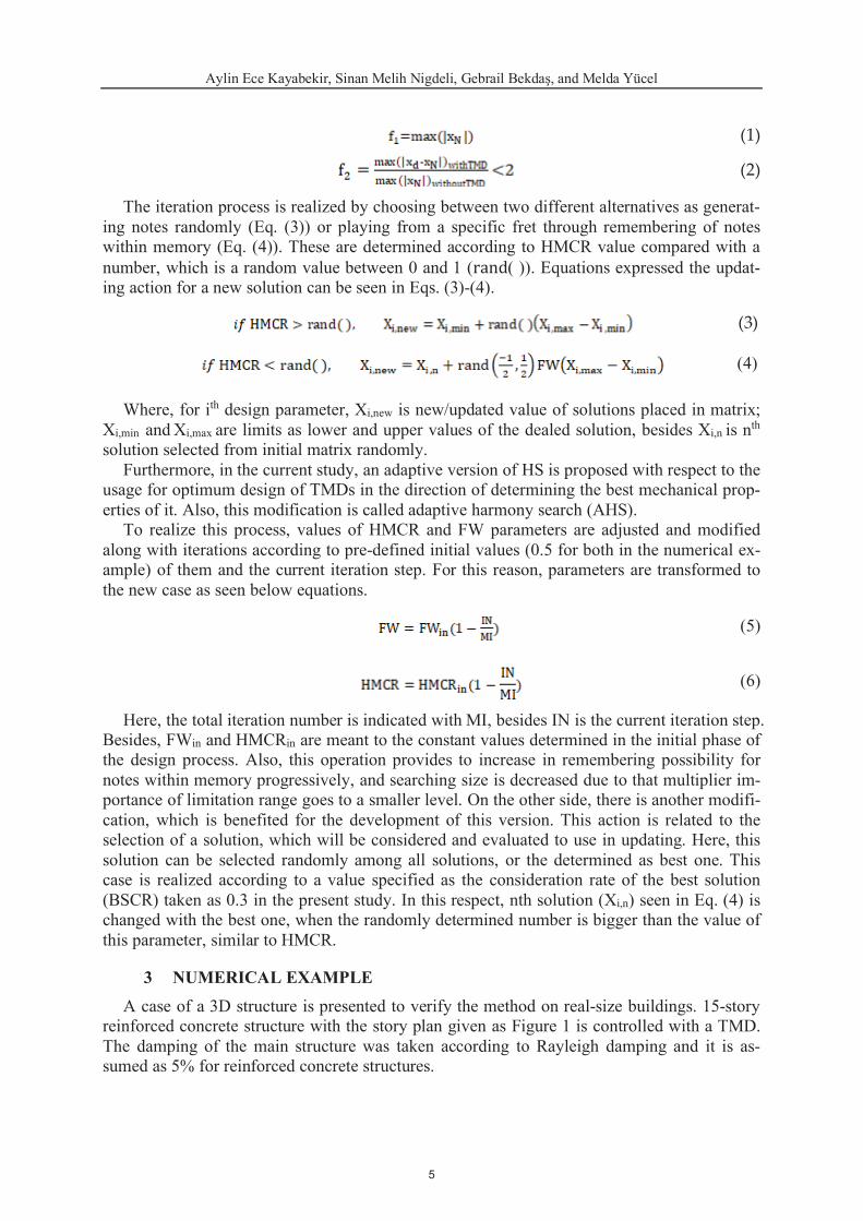
In the study, two objectives are considered. As given in Eqs. (1) and (2), the objectives; f1 and f2 are related with the maximum top story displacement (xN) and the stroke capacity of TMD. f1 is minimized and f2 must be lower than a user-defined value that is taken as 2 in the present study. xd is the displacement of TMD with respect to the ground.
Then the iteration process starts and it is done for several iterations (200 in the numerical example). All results corresponding candidate solutions are checked according to the follow-ing procedure. First, f2 values are checked to minimize if both new and existing solutions ex-ceed the limit taken as 2. If one of them is smaller than 2, it is taken as the best. If both f2 values are lower than 2, f1 is considered in the optimization.
4
(1)
(2)
The iteration process is realized by choosing between two different alternatives as generat-ing notes randomly (Eq. (3)) or playing from a specific fret through remembering of notes within memory (Eq. (4)). These are determined according to HMCR value compared with a number, which is a random value between 0 and 1 (rand( )). Equations expressed the updat-ing action for a new solution can be seen in Eqs. (3)-(4).
(3)
(4)
Where, for ith design parameter, Xi,new is new/updated value of solutions placed in matrix; Xi,min and Xi,max are limits as lower and upper values of the dealed solution, besides Xi,n is nth solution selected from initial matrix randomly.
Furthermore, in the current study, an adaptive version of HS is proposed with respect to the usage for optimum design of TMDs in the direction of determining the best mechanical prop-erties of it. Also, this modification is called adaptive harmony search (AHS).
To realize this process, values of HMCR and FW parameters are adjusted and modified along with iterations according to pre-defined initial values (0.5 for both in the numerical ex-ample) of them and the current iteration step. For this reason, parameters are transformed to the new case as seen below equations.
(5)
(6)
Here, the total iteration number is indicated with MI, besides IN is the current iteration step. Besides, FWin and HMCRin are meant to the constant values determined in the initial phase of the design process. Also, this operation provides to increase in remembering possibility for notes within memory progressively, and searching size is decreased due to that multiplier im-portance of limitation range goes to a smaller level. On the other side, there is another modifi-cation, which is benefited for the development of this version. This action is related to the selection of a solution, which will be considered and evaluated to use in updating. Here, this solution can be selected randomly among all solutions, or the determined as best one. This case is realized according to a value specified as the consideration rate of the best solution (BSCR) taken as 0.3 in the present study. In this respect, nth solution (Xi,n) seen in Eq. (4) is changed with the best one, when the randomly determined number is bigger than the value of this parameter, similar to HMCR.
3 NUMERICAL EXAMPLE A case of a 3D structure is presented to verify the method on real-size buildings. 15-story
reinforced concrete structure with the story plan given as Figure 1 is controlled with a TMD. The damping of the main structure was taken according to Rayleigh damping and it is as-sumed as 5% for reinforced concrete structures.
5

Aylin Ece Kayabekir, Sinan Melih Nigde
A2
A2
E1 E1
D1 D1
C1 C1
B1 B1
A1 A1
F1 F1
G1 G1
H1 H1
I1 I1
J1
B2 C2 D2 E2 F2 G2 H2 I2
J1
J2
J2
J3
J3
J4
J4
B2 C2 D2 E2 F2 G2 H2 I2
Figure 1: The story plan of reinforced concrete structure.
The 3D structure has 9 gridlines with equal distances between them in both directions. The distance between is 8 m and the height of each story is 3.5 m. The rigidity of the structure in both translational directions was calculated as 5520MN/m. The structure has a 3590-ton story mass.
The mass of TMD is taken as 2% of the total mass of the structure. The value of it is 1077 tons. The optimum values such as Td d are found as 1.6770 and 0.1644, respectively. The value of f1 and f2 for the optimum results are 0.3928 m and 1.9991, respectively. The maxi-mum displacement under a set of earthquake records is between 0.0425 m and 0.4638 m for the uncontrolled structure. For the structure with optimum TMD, the maximum displacement is changed between 0.0381 m and 0.3928 m. The most critical excitation is the MUL009 component of the 1994 Northridge earthquake. The time-history plot for the top story dis-placement is shown in Figure 2.
0 5 10 15 20 25 30 35
Time (s)
-0.5
-0.4
-0.3
-0.2
-0.1
0
0.1
0.2
0.3
0.4
x1
5 (m
)
without TMD
with TMD
Figure 2: Time-history plot for the critical excitation.
6

4 CONCLUSIONS The aim of this study is to both present applications of a TMD on a real-size structure and
an improved metaheuristic method for this application. According to the results, the optimiza-tion is effective and it can be seen from the reduction of the objective function values by 15.3%. As seen from the time-history plot given for the most critical excitation, TMD is also effective on rapid damping and the effect of TMD is significant on the peak vibration with the most amplitude, but the essential effect is observed in the following peaks. Additionally, TMD is effective for all excitations that were used in the optimization.
REFERENCES [1] H. Frahm, Device for damping of bodies. Washington, DC: U.S. Patent No: 989,958,
1911. [2] J. Ormondroyd, J.P. Den Hartog, The theory of dynamic vibration absorber, Transac-
tions of the ASME, 50, 922, 1928. [3] H.K. Miyamoto, A.S.J. Gilani , Innovative seismic retroit of an iconic
building. Seventh National Conference on Earthquake Engineering, Istanbul, Turkey, May 30-June 3, 2011.
[4] J.P. Den Hartog, Mechanical vibrations. McGraw- [5] R.E.D. Bishop, D.B. Welbourn, The problem of the dynamic vibration absorber. Engi-
neering, London, 174-769, 1952. [6] K.C. Falcon, B.J. Stone, W.D. Simcock, C. Andrew, Optimization of vibration absorb-
ers: a graphical method for use on idealized systems with restricted damping, Journal Mechanical Engineering Science, 9, 374381, 1967.
[7] G.B. Warburton, Optimum absorber parameters for various combination of response and excitation parameters, Earthquake Engineering and Structural Dynamics, 10, 381401, 1982.
[8] F. Sadek, B. Mohraz, A.W. Taylor, R.M. Chung, A method of estimating the parameters of tuned mass dampers for seismic applications, Earthquake Engineering and Structural Dynamics, 26, 617635, 1997.
[9] M.N.S. Hadi, Arfiadi, Optimum design of absorber for MDOF structures, Journal of Structural Engineering-ASCE, 124, 12721280, 1998.
[10] G.C. Marano, R. Greco, B. Chiaia, A comparison between different optimization crite-ria for tuned mass dampers design, Journal of Sound and Vibration, 329, 4880-4890, 2010.
[11] S. Pourzeynali, S. Salimi, H.E. Kalesar, Robust multi-objective optimization design of TMD control device to reduce tall building responses against earthquake excitations us-ing genetic algorithms, Scentia Iranica, 20, 2, 207-221, 2013.
[12] N.B. Desu, S.K. Deb, A. Dutta, Coupled tuned mass dampers for control of coupled vi-brations in asymmetric buildings, Structural Control and Health Monitoring, 13, 897-916, 2006.
7

Aylin Ece Kayabekir, Sinan Melih Nigde
[13] J.F. Jiménez-Alonso, A. Sáez, Robust optimum design of tuned mass dampers to miti-gate pedestrian-induced vibrations using multi-objective genetic algorithms, Structural Engineering International, 27(4), 492-501, 2017.
[14] . Leung, H. , C.C. Cheng, Lee, Particle swarm optimization of TMD by non-stationary base excitation during earthquake, Earthquake Engineering and Structural Dynamics, 37, 1223-1246, 2008.
[15] , Particle swarm optimization of tuned mass dampers, Engi-neering Structures, 31, 715-728, 2009.
[16] M. Fahimi-Farzam, B. Alinejad, Optimum design of tuned mass damper under base ex-citation using metaheuristic algorithm, 16th European Conference on Earthquake Engi-neering, Thessaloniki, Greece, June 18-21, 2018.
[17] S.M. Nigdeli, G. Optimum tuned mass damper design in frequency domain for structures, KSCE Journal of Civil Engineering, 21, 3, 912-922, 2017.
[18] H. L.J. Tuned mass damper system of high-rise intake towers opti-mized by improved harmony search algorithm, Engineering Structures, 138, 270-282, 2017.
[19] S.M. Nigdeli, G , A. Metaheuristic based optimization of tuned mass dampers on single degree of freedom structures subjected to near fault vibrations, Inter-national Conference on Engineering and Natural Sciences (ICENS 2017), Budapest, Hungary, May 3-7, 2017.
[20] G. , A.E. Kayabekir, S.M. Nigdeli, C. Toklu, Tranfer function amplitude min-imization for structures with tuned mass dampers considering soil-structure interaction, Soil Dynamics and Earthquake Engineering, 116, 552-562, 2019.
[21] A. Farshidianfar, S. Soheili, ABC optimization of TMD parameters for tall buildings with soil structure interaction, Interaction and Multiscale Mechanics, 6, 339-356, 2013.
[22] M. Khatibinia, H. Gholami, R. Kamgar, Optimal design of tuned mass dampers subject-ed to continuous stationary critical excitation, International Journal of Dynamics and Control, 6, 3, 1094-1104, 2018.
[23] S. Etedali, H. Rakhshani, Optimum design of tuned mass dampers using multi-objective cuckoo search for buildings under seismic excitations, Alexandria Engineering Journal, 57, 4, 3205-3218, 2018.
[24] G. , S.M. Nigdeli, X.S. A novel bat algorithm based optimum tuning of mass dampers for improving the seismic safety of structures, Engineering Structures, 159, 89-98, 2018.
[25] S.M. Nigdeli, G , X.S Optimum tuning of mass dampers by using a hy-brid method using harmony search and flower pollination algorithm. In: Del Ser J. (eds) Harmony Search Algorithm. ICHSA 2017. Advances in Intelligent Systems and Com-puting, Vol. 514, Springer, Singapore, 222-231, 2017.
[26] S.M. Nigdeli, G. Optimum design of multiple positioned tuned mass dampers for structures constrained with axial force capacity, The Structural Design of Tall and Special Buildings, 28, 5, e1593, 2019.
8

[27] S.M. Nigdeli, G Teaching-learning-based optimization for estimating tuned mass damper parameters, 3rd International Conference on Optimization Techniques in Engineering (OTENG '15), Rome, Italy, November 7-9, 2015.
[28] M. , G. , S.M. Nigdeli, S. Sevgen, Estimation of optimum tuned mass damper parameters via machine learning, Journal of Building Engineering, 26, 100847, 2019.
[29] .W. Geem, J.H. Kim, G.V. Loganathan, A new heuristic optimization algorithm: har-mony search, Simulation, 76, 2, 60–68, 2001.
[30] FEMA P-695. Quantification of Building Seismic Performance Factors. Washington. [31] The MathWorks Inc MATLAB R2010a. Natick, MA; USA, 2010.
9

OPTIMUM DESIGN OF REINFORCED CONCRETE RETAINING WALLS BY USING SPECIFIC PARAMETER-FREE METAHEURISTIC
ALGORITHMS
Melda Yücel1, 1, Sinan Melih Nigdeli1 and Aylin Ece Kayabekir1
1 Department of Civil Engineering, Istanbul University -
e-mail: [email protected], [email protected], [email protected], [email protected]
Abstract
In the optimum design of structural systems, the robustness and the performance are related to the best tuning of the parameters of the method. For metaheuristic algorithms inspired by phe-nomena in life, algorithm-specific parameters exist in addition to general parameters that are the population of the generated candidate solution and the number of iterations that are needed to find the final optimum solution. In the optimum design of reinforced concrete (RC) structures, the dimensions are optimized by considering the minimization of the total cost. These problems are highly constrained by the design requirements presented in design codes. Especially, RC retaining walls involve the check of stability conditions as geotechnical state limits in addition to structural state limits. This situation makes the optimization problem challenging. A better and robust algorithm is always in search. In the present study, two specific parameter-free metaheuristic algorithms are employed. These algorithms are teaching-learning-based optimi-zation (TLBO) and Jaya algorithm (JA). Since JA is a single-phase algorithm and both phases of TLBO defined as teacher and learner phases are consequently applied, a switch probability is not needed. Also, the existing factor is defined randomly. These two algorithms were tested on three cases and the results were compared with three classical algorithms such as Genetic Algorithm (GA), Differential Evaluation (DE), and Particle Swarm Optimization (PSO). In this verification, JA needs less function evaluation to reach the optimum results. As conclusions, both TLBO and JA are robust methods for the optimization problem.
Keywords: Reinforced Concrete, Retaining Walls, Optimization, Metaheuristic Algorithms
EUROGEN 2021 14th ECCOMAS Thematic Conference on
Evolutionary and Deterministic Methods for Design, Optimization and Control N. Gauger, K. Giannakoglou, M. Papadrakakis, J. Periaux (eds.)
Streamed from Athens, Greece, – 2021
10

Melda Yücel, Gebrail Bekda , Sinan Melih Nigdeli and Aylin Ece Kayabekir
1 INTRODUCTION Generally, engineering designs are carried out by taking two main objectives into consider-
ation. The first of these is structural security, the other is cost. Good engineering design can be defined as the best combination or balance of these two objectives. The process in which this balance is investigated is called optimization and the obtained result is called optimum design.
Different methods have been developed and used from past to present in order to find the optimum design in engineering designs. Especially in recent years, metaheuristic algorithms are one of the methods used frequently for this purpose. Metaheuristic algorithms are methods developed by taking inspiration from nature. Examples of these are genetic (GA) [1,2] and differential evolution (DE) [3] algorithms from the evolutionary process, flower pollination (FPA) [4] from the pollination process of flowers, the bat algorithm (BA) [5] from the echolo-cation characteristics of bats, the gray wolf optimization (GWO) [6] from the herd hierarchy and hunting processes of the gray wolves, the particle swarm optimization (PSO) [7] from the herd movement of living things, ant colony optimization (ACO) [8] from the foraging process of ants, teaching-learning-based optimization (TLBO) [9] from the student-teacher relationship and learning in a classroom.
An optimization process is carried out using metaheuristic algorithms in many areas of struc-tural engineering. One of these areas is the optimum design of reinforced concrete structures. Since reinforced concrete structures consist of two different mechanical and cost-effective ma-terials, it is necessary to find a combination that will provide the lowest cost (optimum design) of concrete and steel. The optimum design of RC retaining walls is one of the areas that have been researched extensively. Various metaheuristic methods such as Simulated Annealing (SA) [10,11], PSO [12], Harmony search (HS) [13] Big Bang Big Crunch (BB-BC) [14], Firefly Algorithm (FA) [15], FPA [16] have been used in the design of RC retaining walls. In addition to these studies, there are also studies where performance evaluation of algorithms [17] is per-formed and modified or hybrid algorithms [18] are used.
In this study, the effect of different parameters on optimum RC retaining wall design was investigated. For this purpose, five different metaheuristic algorithm-based methods have been developed. In this way, as a result of the study, the researchers were informed about the effects of parameters as well as the most effective metaheuristic method for optimum design.
2 OPTIMUM DESIGN VIA METAHEURISTIC ALGORITHMS Metaheuristic methods can generally be summarized with 3 stages as given in Fig.1. In the first stage (pre-optimization), the design constants of the problem, the lower and upper
limits of the design variables, the population number (pn), the algorithm-specific parameters and the stopping criteria of the optimization are defined. Then, candidate solutions (totally pn) are generated according to Eq. (1) and stored in initial solution matrix.
= , + ( , , ) (1)
In Eq. (1), , , and , represent ith candidate solution, minimum and maximum limits of ith solution respectively. rand is a function that is generated by random values between 0 and 1.
The second stage is the analysis stage. In this stage, the objective function of each solution is calculated, and the design constraints of the problem are checked. Objective functions of solutions that violate the design constraint are penalized using a penalization value. Within the scope of this study, the objective function is determined as the minimum material cost given as Eq.(2), and for the penalization, a high value is defined.
11

Melda Yücel, Gebrail Bekda , Sinan Melih Nigdeli and Aylin Ece Kayabekir
min ( ) = + (2)
In Eq. (2), Cc and Cs are unit concrete and unit reinforcing steel costs respectively. Vc and Ws represent the volume of the concrete and unit volume weight of the steel, respectively.
At the last stage (optimization stage), an iterative process is started. In this process, first of all new solution matrix is generated according to algorithm equations. In this study, 5 different algorithms, GA, DE, PSO, TLBO and JA were employed and algorithm-specific equations are given below.
Equation of genetic algorithm (GA):
, = > , , + , , (3)
In Eq. (3), mr is mutation rate, q is a gene (design parameter) randomly-selected from the total design parameter. , , , and , are new design variable, lower and upper limit values of qth design variable, respectively. Unlike GA, DE uses two equations (Eq. 4 and 5). New design variables are derived by selecting one of these two equations according to DE rules.
, = , + , , (4)
X , = X , {if rand CR or cs = rand (5)
In Eq. (4 and 5), X , , X , , X , represent randomly selected different solutions and F is the weighting factor. CR, cs, and randcs are crossover possibilities, current candidate solution, and randomly selected solution.
In PSO, new values are found by using a single equation as in GA. This equation as follows
, = , + , (6)
where , is the current position of jth particle and , can be calculated with Eq. (7).
, = , + , , + , , (7)
In Eq. (7), , is current velocity jth particle. , and , represent values of the best global and local positions respectively. and are positive constant parameters used to con-trol velocity.
In the TLBO algorithm, two different equations are used in generating new solutions. How-ever, unlike other two-equation algorithms, it uses both of the equations one after the other instead of choosing one of the equations. These equations are as follows
X , = X , + rand X , (TF) X , (8)
, =< , , + , ,
> , , + , , (9)
where X , , X , , X , represent values of existing solution, best solution and mean val-ues of existing solutions respectively, and TF shows teaching factor. X , and X , are randomly selected candidate solutions. Objective functions corresponding to these solutions (X , and X , ) are expressed with OF and OF , respectively.
The other algorithm used in the study, JA uses a single equation given in Eq.(10).
, = , + , , , , (10)
12

Melda Yücel, Gebrail Bekda , Sinan Melih Nigdeli and Aylin Ece Kayabekir
In Eq.(10), , is worst solution in terms of the objective function.
After the generation of new solution matrix, it is done comparation between solution matrix and existing one. In case of new solutions have better objective function value, new solutions replace existing solutions. In case new solutions have better objective function value, the exist-ing solution matrix is updated with new solutions. This process is continued until satisfying stopping criteria of the problem. In this study maximum iteration number is determined as stop-ping criteria.
Figure 1: The optimization flowchart
A
NA
LYSI
S TA
GE
OPT
IMIZ
ATI
ON
STA
GE
Violated
PRE-
OPT
IMIZ
ATI
ON
STA
GE
Not Provided
Provided
Not Violated
Define design constants, design variable ranges, population and algorithm-specific parameters
Choose a type of modification
STOP
START
Generation of an initial solution matrix including candidate variables
Calculate objective functions
Modify existing candidate solutions and update solution matrix
Calculate design constraints and check violation
Penalize objective function
Check stopping criteria
13
Melda Yücel, Gebrail Bekda , Sinan Melih Nigdeli and Aylin Ece Kayabekir 3 NUMERICAL EXAMPLE
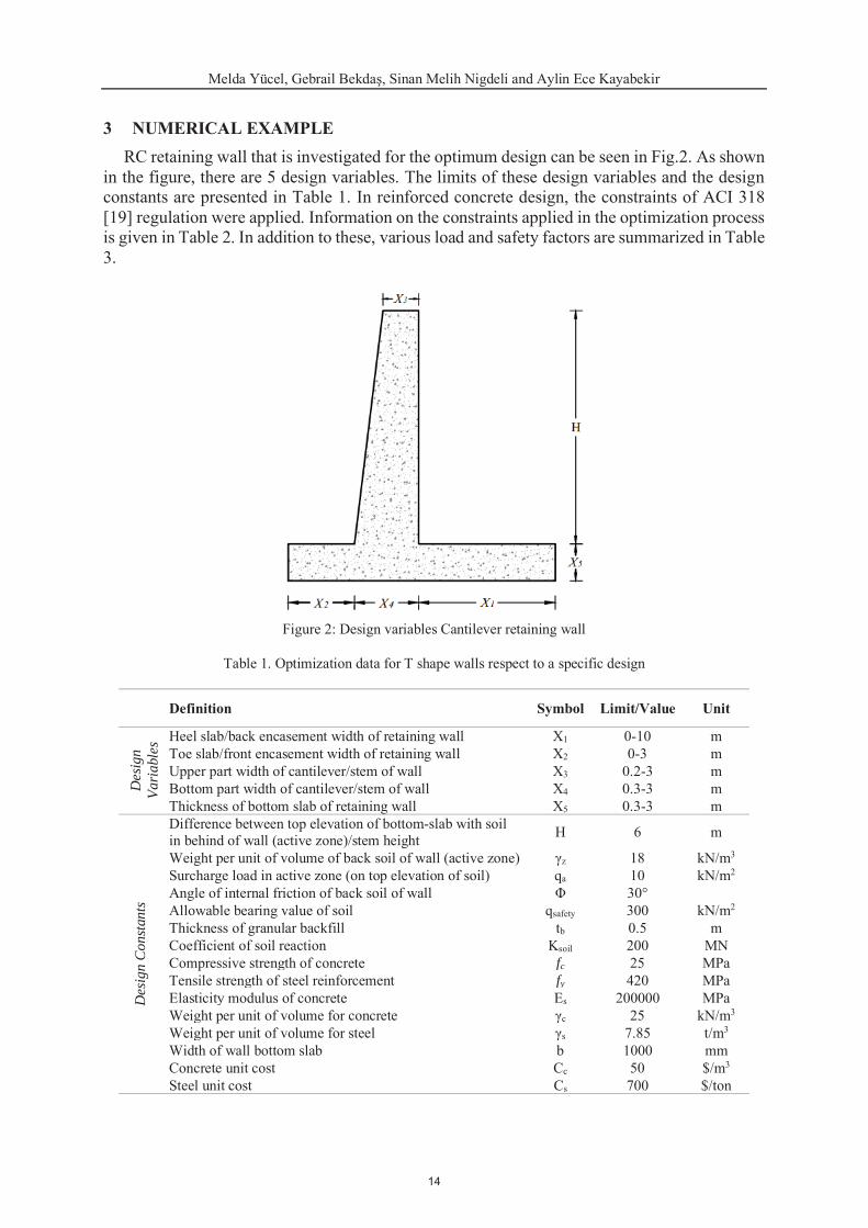
RC retaining wall that is investigated for the optimum design can be seen in Fig.2. As shown in the figure, there are 5 design variables. The limits of these design variables and the design constants are presented in Table 1. In reinforced concrete design, the constraints of ACI 318 [19] regulation were applied. Information on the constraints applied in the optimization process is given in Table 2. In addition to these, various load and safety factors are summarized in Table 3.
Figure 2: Design variables Cantilever retaining wall
Table 1. Optimization data for T shape walls respect to a specific design
Definition Symbol Limit/Value Unit
Des
ign
Vari
able
s Heel slab/back encasement width of retaining wall X1 0-10 m Toe slab/front encasement width of retaining wall X2 0-3 m Upper part width of cantilever/stem of wall X3 0.2-3 m Bottom part width of cantilever/stem of wall X4 0.3-3 m Thickness of bottom slab of retaining wall X5 0.3-3 m
Des
ign
Con
stan
ts
Difference between top elevation of bottom-slab with soil in behind of wall (active zone)/stem height H 6 m
Weight per unit of volume of back soil of wall (active zone) z 18 kN/m3 Surcharge load in active zone (on top elevation of soil) qa 10 kN/m2 Angle of internal friction of back soil of wall 30° Allowable bearing value of soil qsafety 300 kN/m2 Thickness of granular backfill tb 0.5 m Coefficient of soil reaction Ksoil 200 MN Compressive strength of concrete fc 25 MPa Tensile strength of steel reinforcement fy 420 MPa Elasticity modulus of concrete Es 200000 MPa Weight per unit of volume for concrete c 25 kN/m3 Weight per unit of volume for steel s 7.85 t/m3 Width of wall bottom slab b 1000 mm Concrete unit cost Cc 50 $/m3 Steel unit cost Cs 700 $/ton
14

Melda Yücel, Gebrail Bekda , Sinan Melih Nigdeli and Aylin Ece Kayabekir
Table 2. The design constraints
Description Constraints Safety for overturning stability g1(X): FoSot,design ot Safety for sliding g2(X): FoSs,design sSafety for bearing capacity g3(X): FoSbc,design bc Minimum bearing stress (qmin) g4(X): qmin Flexural strength capacities of critical sections (Md) g5-7(X): Md u Shear strength capacities of critical sections (Vd) g8-10(X): Vd u Minimum reinforcement areas of critical sections (Asmin) g11-13(X): As Asmin Maximum reinforcement areas of critical sections (Asmax) g14-16(X): As Asmax
Table 3. ACI 318 Regulation values utilized in optimization process
Load Coefficients in ACI Regulation Symbol Value Coefficient for load increment Cl 1.7 Reduction coefficient for section bending moment capacity FiM 0.9 Reduction coefficient for section axial load capacity FiN 0.9 Reduction coefficient for section shear load capacity FiV 0.75 Constant load coefficient GK 0.9 Live load coefficient QK 1.6 Horizontal load coefficient HK 1.6 Safety coefficient respect to overturning Osafety 1.5 Safety coefficient respect to slipping Ssafety 1.5
Three different case analyses were performed using GA, DE, PSO, TLBO and JA. These cases are as follows:
Case 1: Optimum design variables are investigated using thirty multiple cycles of optimiza-tion. In the optimization process, twenty populations and five thousand iteration numbers are used.
Case 2: Effect of wall height on the optimum design as well as algorithm performances are investigated. As different from Case 1, H is defined as 10m.
Case 3: Best population and iteration number combination are investigated. For this investi-gation, optimization operations are carried out for different maximum iteration numbers from 1 to 5000 by increasing 499 in each step and for different population numbers such as 3, 5, 10, 15, 20, 25, 30.
The optimum results for these cases are shown in Table 4-6, respectively.
Table 4. Optimum design results for Case 1.
Algorithm X1 X2 X3 X4 X5 Min. Cost Ave. Cost Standard Dev. GA 4.1257 0.0003 0.2003 0.6212 0.4274 428.2421 449.3181 36.9566092 DE 4.1323 0.0000 0.2000 0.6098 0.4267 428.1139 433.3653 11.4300331 PSO 4.1322 0.0000 0.2000 0.6099 0.4267 428.1139 449.2315 40.6569904 TLBO 4.1323 0.0000 0.2000 0.6099 0.4267 428.1139 428.1139 0.0000005 JA 4.1323 0.0000 0.2000 0.6099 0.4267 428.1139 428.1139 0.0000012
Table 5. Optimum design results for Case 2.
Algorithm X1 X2 X3 X4 X5 Min. Cost Ave. Cost Standard Dev. GA 6.3735 1.5040 0.2010 1.3299 0.7140 1365.7614 1370.8030 5.8839356 DE 6.3480 1.4917 0.2000 1.3656 0.7086 1365.2365 1442.5197 146.3331618 PSO 6.3482 1.4879 0.2000 1.3655 0.7074 1365.2432 1473.0711 137.6288067 TLBO 6.3479 1.4920 0.2000 1.3658 0.7087 1365.2365 1365.2368 0.0001623 JA 6.3478 1.4919 0.2000 1.3660 0.7087 1365.2367 1371.6683 34.6327849
15

Melda Yücel, Gebrail Bekda , Sinan Melih Nigdeli and Aylin Ece Kayabekir
Table 6. Optimum design values of wall with the best population-iteration combinations
Algorithm X1 X2 X3 X4 X5 Min. Cost Ave. Cost Standard Dev. Iter.Num.
Pop. Num.
GA 4.1304 0.0046 0.2001 0.6106 0.4240 428.2186 428.6384 0.34408003 2995 15 DE 4.1323 0.0000 0.2000 0.6098 0.4267 428.1139 428.1139 0.0000000 1997 30 PSO 4.1324 0.0000 0.2000 0.6096 0.4267 428.1140 699.2741 732.5740371 3993 30 TLBO 4.1323 0.0000 0.2000 0.6098 0.4267 428.1139 428.1139 0.0000126 4991 25 JA 4.1323 0.0000 0.2000 0.6099 0.4267 428.1139 428.1139 0.0000057 4492 25
4 CONCLUSION
4.1 Case 1 DE, PSO, TLBO and JA find close values in terms of objective functions (minimum cost),
whereas GA could not reach the minimum value. Therefore, it can be said that all algorithms except GA are effective in finding the minimum result. However, as seen in Table 4, the stand-ard deviation and average cost values of the DE and PSO algorithms are higher than other ones. Therefore, it can be concluded that TLBO and JA algorithms are more effective and stable for this structural model.
4.2 Case 2 Increasing the wall height from 6m to 10m caused the optimum X2 value, that is found zero
in Case 1. The minimum cost design has been obtained with DE and TLBO algorithms. Besides, it is seen that JA and PSO obtained results very close to these results. Considering all the pa-rameters obtained from the analysis results of the algorithms, it can be said that TLBO is better than the others.
4.3 Case 3 It is seen that all algorithms except GA have reached the optimum value. When all the sta-
tistical values are evaluated together, it is understood that the DE algorithm seems better, but there is no significant difference between the TLBO and JA algorithms. In terms of the number of iterations, the DE algorithm again reaches a slightly faster result. In terms of population numbers, it can be said that 15 to 30 population numbers are the most suitable range for opti-mum analysis.
REFERENCES [1] J.H. Holland, Adaptation in natural and artificial systems, University of Michigan Press,
1975. [2] D. E. Goldberg, Genetic algorithms in search, Optimization and machine learning, Bos-
ton MA: Addison Wesley, 1989. [3] R. Storn, K. Price, Differential evolution–a simple and efficient heuristic for global opti-
mization over continuous spaces. Journal of global optimization, 11(4), 341-359, 1997. [4] X.S. Yang, Flower pollination algorithm for global optimization, International Confer-
ence on Unconventional Computing and Natural Computation, September Heidelberg-Berlin, Springer, 240-249, 2012.
16

Melda Yücel, Gebrail Bekda , Sinan Melih Nigdeli and Aylin Ece Kayabekir
[5] X. S. Yang, A New Metaheuristic Bat-Inspired Algorithm, in: Nature Inspired Coopera-tive Strategies for Optimization (NISCO 2010), Studies in Computational Intelligence, Springer Berlin. 65-74, 2010.
[6] S. Mirjalili, S.M. Mirjalili, A. Lewis, Grey wolf optimizer, Advances in Engineering Soft-ware, 69, 46-61, 2014.
[7] J. Kennedy, R.C. Eberhart, Particle swarm optimization. In: Proceedings of IEEE Inter-national Conference on Neural Networks No. IV, Perth Australia; November 27 - Decem-ber 1. 1942–1948, 1995.
[8] M. Dorigo, V. Maniezzo, A. Colorni, The ant system: Optimization by a colony of coop-erating agents. IEEE Transactions on Systems Man and Cybernet B 26, 29–41, 1996.
[9] R.V. Rao, V.J. Savsani, D.P. Vakharia, Teaching–learning-based optimization: A novel method for constrained mechanical design optimization problems, Computer-Aided De-sign, 43, 303–315, 2011.
[10] B. Ceranic, C. Fryer, R.W. Baines, An application of simulated annealing to the optimum design of reinforced concrete retaining structures, Computers & Structures, 79(17) 1569-1581, 2001.
[11] V. Yepes, J. Alcala, C. Perea, F. Gonzalez-Vidosa, A parametric study of optimum earth-retaining walls by simulated annealing, Engineering Structures, 30(3) 821-830, 2008.
[12] B. Ahmadi-Nedushan, H. Varaee, Optimal Design of Reinforced Concrete Retaining Walls using a Swarm Intelligence Technique, The first International Conference on Soft Computing Technology in Civil, Structural and Environmental Engineering, Stirling-shire, Scotland, 2009.
[13] A. Kaveh, A.S.M. Abadi, Harmony search based algorithms for the optimum cost design of reinforced concrete cantilever retaining walls, International Journal of Civil Engineer-ing, 9(1) 1-8, 2011.
[14] C. V. Camp, A. Akin, Design of Retaining Walls Using Big Bang-Big Crunch Optimiza-tion, Journal of Structural Engineering, ASCE, 138(3) 438-448, 2012.
[15] R. Sheikholeslami, B. Gholipour Khalili, S.M. Zahrai, Optimum Cost Design of Rein-forced Concrete Retaining Walls Using Hybrid Firefly Algorithm, International Journal of Engineering and Technology, 6(6) 465-470, 2014.
[16] P.E. Mergos, F. Mantoglou, Optimum design of reinforced concrete retaining wall with the flower pollination algorithm, Structural and Multidisciplinary Optimization, 2019, https://doi:10.1007/s00158-019-02380-x.
[17] A.H. Gandomi, A.R. Kashani, D.A. Roke, M. Mousavi, Optimization of retaining wall design using recent swarm intelligence techniques. Engineering Structures, 103, 72-84, 2015.
[18] R. Sheikholeslami, B.G. Khalili, A. Sadollah, J. Kim, Optimization of reinforced concrete retaining walls via hybrid firefly algorithm with upper bound strategy. KSCE Journal of Civil Engineering, 20(6), 2428-2438, 2016.
[19] Building Code Requirements for Structural Concrete and Commentary, (2014). ACI Committee, ACI 318.
17

NEW MODIFICATIONS OF TEACHING FACTOR IN TEACHING-LEARNING-BASED OPTIMIZATION FOR STRUCTURAL
MECHANICS 1, and Sinan Melih Nigdeli1
1 Department of Civil Engineering, Istanbul University -
e-mail: [email protected], [email protected]
Abstract
Teaching-learning-based optimization (TLBO) is a metaheuristic algorithm that simulates the two phases of education. These two phases namely the teacher and learner phases are conse-quently done in the optimization processes because in real life, the education with a teacher continues with the self-learning of students by sharing knowledge and information in class. TLBO is a user-defined-free algorithm, but it contains randomly defined parameters such as teaching factor (TF). TF can only take integer numbers and it is randomly chosen as 1 or 2. In this study, TF is modified as real numbers and an adaptive limitation is applied for the maximum value of TF. The algorithm is applied to various structural mechanics problems that are used benchmark structural optimization problems. The investigated problems are the weight optimization of cantilever beams and the minimization of total material and construc-tion cost of a tubular column problem. The modification to the TF plays an important role in the local optima problem.
Keywords: Structural Optimization, Teaching-Learning-Based optimization, Optimization, Metaheuristic Algorithms, Teaching Factor
EUROGEN 2021 14th ECCOMAS Thematic Conference on
Evolutionary and Deterministic Methods for Design, Optimization and Control N. Gauger, K. Giannakoglou, M. Papadrakakis, J. Periaux (eds.)
Streamed from Athens, Greece, – 2021
18

G Sinan Melih Nigdeli
1 INTRODUCTION In engineering, there are two processes which are analysis and design. Firstly, the mathe-
matical model of the engineering problem is analyzed, and then it is designed according to the requirement that provides safety and demands of the users. In design, this process is compli-cated in finding the best possible design due to existing constraints. These constraints reflect user demands and design regulations that formalize the safety factors for maximum displace-ment, stress, slenderness, and the required ductility in structural engineering. A good engineer has the goal of finding the best economical solutions. In that case, the design problem is a minimization problem of the total cost (or weight of the material) and it is a nonlinear one due to existing of constraints. In that case, metaheuristic algorithms are an excellent choice to make an iterative process to optimize the design.
Metaheuristic algorithms imitate phenomena in life and formulate them as several phases of an iterative process. According to Sorensen et al. [1], there are five periods of metaheuristic starting in the 1940s and now, we are in the framework-centric period. In this period, the number of metaheuristic shows a great increase, but these methods are criticized due to simi-larity to each other. The only difference is to use a different metaphor. Examples of metaphors of the best-known methods are natural evaluation in the genetic algorithm (GA) [2-3], musical performances in harmony search (HS) [4], the behavior of ants in ant colony optimization (ACO) [5], reproduction process flowers in flower pollination algorithm (FPA) [6], sensing ability of bats in Bat Algorithm (BA) [7] and teaching-learning process in teaching-learning-based optimization (TLBO) [8].
In the present study, TLBO was modified for solving structural optimization problems. The modified teaching factor of TLBO is presented on two benchmark problems.
2 THE OPTIMIZATION METHODOLOGY TLBO was developed by Rao et al. [8] as a parameter-free metaheuristic algorithm. The
two phases of education such as the teacher phase done via the guide of a teacher and the stu-dent phase via self-study are formulated and consequently applied.
The main optimization process of a constrained engineering problem is given in Fig. 1. Af-ter the definition of the problem, an initial solution matrix is generated by assigning random solutions for the design variables. Then the essential optimization starts. In the analysis stage that is done after assigning a set of design variables, design constraints are checked and the objective function is penalized if a violation exists. In the present study, the violated solutions are assigned as a big value as 106. The optimization process continues for a maximum number of iterations as the stopping criteria of the problems.
In the TLBO, the teacher and learner phases are consequently applied. The comparison of the results is done via the value of the objective function.
The teacher phase is formulated as Eq. (1). TF is called the teaching factor and it can take integer number 1 or 2, randomly. In the present study, TF can be real numbers and it is formu-lated as Eq. (2).
t 1 t *i i avex x rand(1)(g TFx ) (1)
max minmax
(TF TF )TF TF tmax iter
(2)
19

Nigdeli
AN
ALY
SIS
TAG
E O
PTIM
IZA
TIO
N S
TAG
E
Violated
PRE-
OPT
IMIZ
ATI
ON
STA
GE
Not Provided
Provided
Not Violated
Define design constants, design variable ranges, population and algorithm-specific parameters
Choose a type of modification
STOP
START
Generation of an initial solution matrix including candidate variables
Calculate objective functions
Modify existing candidate solutions and update solution matrix
Calculate design constraints and check violation
Penalize objective function
Check stopping criteria
Figure 1: The optimization flowchart
20
G Sinan Melih Nigdeli
In Eq. (1), xit+1 is the ith set of (t+1)th iteration, while xi
t is the existing one of the tth itera-tion. A random number between 0 and 1 is shows as rand(1), g* and xave are the best solution (teacher) and the average of all solutions. In Eq. (2), TFmax and TFmin are the minimum and maximum value of TF. In the present study, TFmax and TFmin are taken as 2 and 1, which are limits of classical TLBO method. The maximum iteration number and current iteration num-ber are shown as maxiter and t, respectively.
The student phase is formulated in Eq. (3). In this phase, two existing solutions (random chosen k and j) are used according to objective function (f(x)).
)()())(1(
)()())(1(1tk
tj
tj
tk
ti
tk
tj
tk
tj
tit
ixfxfifxxrandx
xfxfifxxrandxx (3)
3 NUMERICAL EXAMPLES
3.1. COST OPTIMIZATION OF TUBULAR COLUMN UNDER COMPRESSIVE LOAD
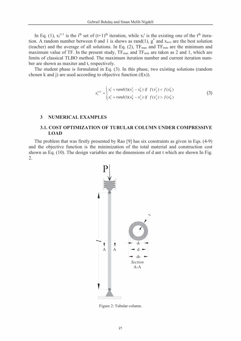
The problem that was firstly presented by Rao [9] has six constraints as given in Eqs. (4-9) and the objective function is the minimization of the total material and construction cost shown as Eq. (10). The design variables are the dimensions of d ant t which are shown In Fig. 2.
Figure 2: Tubular column.
21
Nigdeli
The design y), elasticity modulus 2, 0.85x10⁶ 2,
0.0025 kgf 3, and 250 cm, respectively.
011ydt
Pg (4)
01)(
8223
2
2 tdEdtPlg (5)
012
3 dg (6)
01
144dg (7)
012.0
5 tg (8)
01
8.06tg (9)
ddttdf 28.9),( (10)
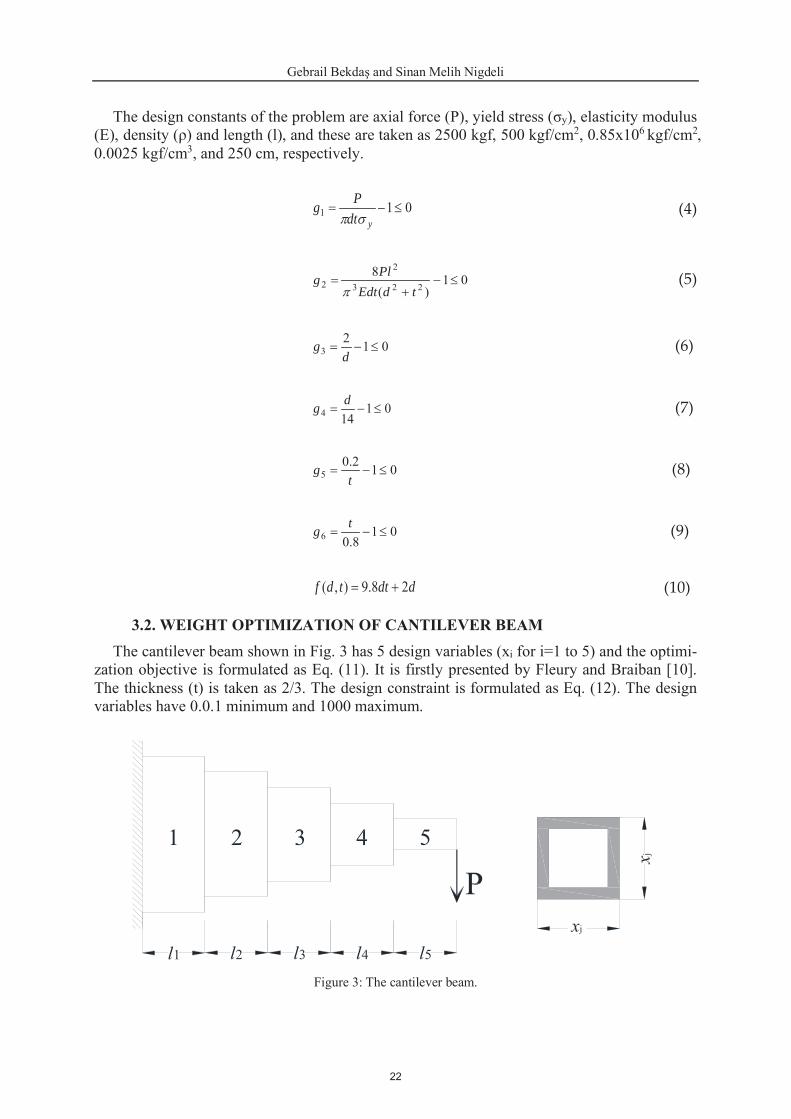
3.2. WEIGHT OPTIMIZATION OF CANTILEVER BEAM The cantilever beam shown in Fig. 3 has 5 design variables (xi for i=1 to 5) and the optimi-
zation objective is formulated as Eq. (11). It is firstly presented by Fleury and Braiban [10]. is formulated as Eq. (12). The design
variables have 0.0.1 minimum and 1000 maximum.
Figure 3: The cantilever beam.
22

G Sinan Melih Nigdeli
)(0624.0)( 54321 xxxxxxfMinimize j (11)
011719376135
34
33
32
31
1 xxxxxg (12)
4 REUSLTS AND CONCLUSIONS
The optimum results for the tubular column problem are shown in Table 1. According to the results, the modified TLBO is also effective to find the same results as TLBO. Also, the average value is the same as the best one for 30 cycles of optimization. It leads to a small standard deviation (std) value.
Table 1: The optimum results of tubular column problem
TLBO Modified TLBO t 0.291965 0.291965 d 5.451156 5.451156 f(x) (best) 26.4995 26.4995 f(x) (ave) 33358.95 26.4995 std 1.83x10⁵ 1.81x10⁻¹⁴
The classical TLBO has a very big average and std values due to trapping a local optimum in one of the optimization cycles. In a cycle, TLBO was not effective to find a final result without violating the design constraints and it was penalized. The convergence plot is also given for the tubular column problem in Fig. 4. As seen from the plot, modified TLBO has the advantage of finding exact optimum results quickly.
10 0 10 1 10 2
t
26
27
28
29
30
31
32
33
f(x)
TLBO
Modified TLBO
Figure 4: The convergence plot for the tubular column problem
The optimum results for the cantilever problem are shown in Table 2. For the cantilever beam problem, modified TLBO and classical TLBO have similar results. As seen from Fig. 5, the modified TLBO has the same effect that is seen after the 30th iteration.
23

Nigdeli
Table 2: The optimum results of cantilever beam problem
TLBO Modified TLBO x1 6.01588339 6.01592868 x2 5.30936515 5.30929444 x3 4.49365821 4.49390785 x4 3.50171404 3.50159740 x5 2.15303927 2.15293149 f(x) (best) 1.33995639 1.33995638 f(x) (ave) 1.33995642 1.33995641 Std 0.00000003 0.00000003
10 0 10 1 10 2
t
26
27
28
29
30
31
32
33
f(x)
TLBO
Modified TLBO
Figure 5: The convergence plot for the cantilever beam problem
As conclusion, the modification of using real numbers for TF is effective in finding global optimum results. The classical version of TLBO is also effective on structural optimization, but the optimum results may not be found in a cycle of optimization since it may trap to local optimum. Using real numbers for TF eliminates this problem. In this study, the modification was tested for benchmark structural engineering problems. This study may be enlarged to the more complicated structural design optimization problem.
REFERENCES [1] Sörensen, K., Sevaux, M., & Glover, F. (2018). A history of metaheuristics. Handbook
of heuristics, 1-18. [2] Holland, J.H., 1975. Adaptation in Natural and Artificial Systems. University of Michi-
gan Press, Ann Arbor, Michigan. [3] Goldberg, D.E., Samtani, M.P. (1986). Engineering optimization via genetic algorithm.
Proceedings of Ninth Conference on Electronic Computation. ASCE, New York, NY, pp. 471-482.
[4] Geem, Z.W., Kim, J.H., Loganathan, G.V., 2001. A new heuristic optimization algo-rithm: harmony search. Simulation 76, 60–68.
24

G Sinan Melih Nigdeli
[5] Dorigo, M., Maniezzo, V., Colorni, A., 1996. The ant system: Optimization by a colony of cooperating agents. IEEE Transactions on Systems Man and Cybernet B 26, 29–41.
[6] Yang, X. S. (2012), Flower pollination algorithm for global optimization, in: Unconven-tional Computation and Natural Computation 2012, Lecture Notes in Computer Science, Vol. 7445, pp. 240-249.
[7] Yang, X. S. (2010). A new metaheuristic bat-inspired algorithm. Nature inspired coop-erative strategies for optimization (NICSO 2010), 65-74.
[8] Rao, R. V., Savsani, V. J., & Vakharia, D. P. (2011). Teaching–learning-based optimi-zation: a novel method for constrained mechanical design optimization prob-lems. Computer-Aided Design, 43(3), 303-315.
[9] Rao, S. S. (1996), Engineering optimization: theory and practice, 3rd edn. John Wiley & Sons, Chichester.
[10] Fleury, C., Braibant, V. (1986), Structural optimization: a new dual method using mixed variables, Int J Numer Meth Eng 23, 409-428
25

THE EFFECT OF THE ASSUMED INHERENT DUMPING IN THE TUNING OF TUNED MASS DAMPERS
Ayla Ocak1, Gebrail 1 and Sinan Melih Nigdeli
1 Department of Civil Engineering, Istanbul University - Cerrahpasa ,Istanbul, Turkey
e-mail: [email protected], [email protected], [email protected]
Abstract
As known, the damping ratio of structures is assumed as a constant value. This constant value is also used in the analysis of structures and these analysis results are used in the optimum design of active and passive control systems. In the present study, the assumed value of inherent damping of the structure is tested on tuned mass dampers that are used in the structures to reduce responses resulting from earthquakes. For this purpose, three methods are investigated by considering the increase or decrease of the damping coefficient of the superstructure. The first method is the usage of equations of Den Hartog which does not consider the inherent dumping of the structure. Secondly, the basic equations of Sadek et al. that include the inherent dumping for the optimum parameters are examined. Finally, a metaheuristic-based optimiza-tion approach using the Jaya algorithm (JA) was used in the investigation.
Keywords: Optimization, Dumping, Tuned Mass Dampers, Jaya Algorithm.
EUROGEN 2021 14th ECCOMAS Thematic Conference on
Evolutionary and Deterministic Methods for Design, Optimization and Control N. Gauger, K. Giannakoglou, M. Papadrakakis, J. Periaux (eds.)
Streamed from Athens, Greece, – 2021
26

1 INTRODUCTION Mass dampers are devices that Hermann Frahm [1] invented in 1909 to prevent machine
vibration on board, in which Ormondroyd and Den Hartog [2] put forward the first theoretical studies for this type of damper. The fact that TMDs became a part of the design took its place in architecture with research by Mcnamara [3]. Considering the mass of the structure on which TMDs are placed, SDOF has a mass of approximately 5% of the structure for a structure [4-5]. Similar to other passive damping systems, these systems, which convert mechanical energy to damping energy as a working principle, have become a preferred system for building vibration control in terms of not needing external energy, easy cost and maintenance and applicability to old buildings. Looking at the areas of use, we can see that the bridge, tower, etc. exposed to wind forces. It is seen that it is placed in structures, earthquake-effect structures and in the types of structures that are negativized by other vibrations. An example is folded pendulum with a movement ampliated capacity of ±48 cm, with a mass ratio of 4.5%, to 450 tons for the 40-storey Socar Tower (Figure 1 and 2), which was built in 2010, in Baku, capital of Azerbaijan. Another example used in TMD, Alphabetic Tower (Figure 3) in Batumi, Georgia, used standard TMD with a 3.5% mass ratio of 62.85 tons with a movement amplitude of ±24cm [6].
Figure 1. Socar Tower [7]
Figure 2. Socar Tower Folded Pendilum TMD [8]
27
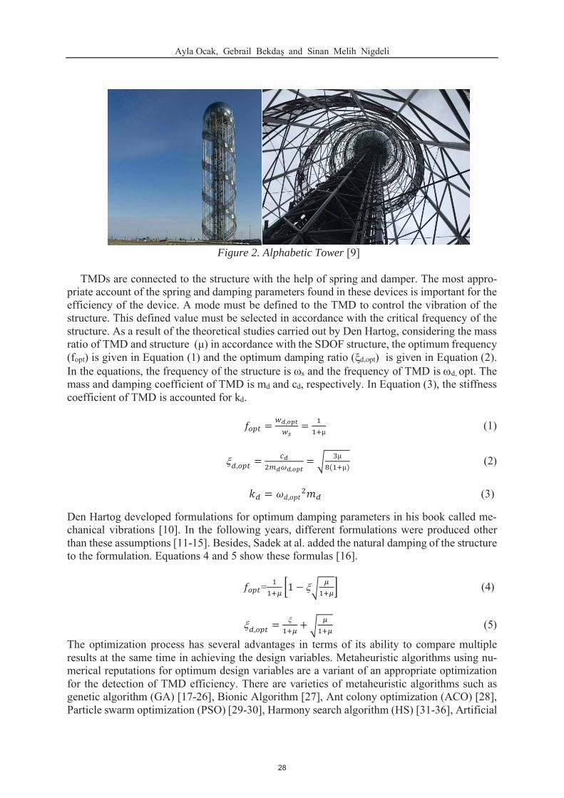
Figure 2. Alphabetic Tower [9]
TMDs are connected to the structure with the help of spring and damper. The most appro-priate account of the spring and damping parameters found in these devices is important for the efficiency of the device. A mode must be defined to the TMD to control the vibration of the structure. This defined value must be selected in accordance with the critical frequency of the structure. As a result of the theoretical studies carried out by Den Hartog, considering the mass ratio of TMD and structure e with the SDOF structure, the optimum frequency (fopt) is given in Equation (1) and the optimum damping ratio d,opt) is given in Equation (2). In the equations, the frequency of the structure is s and the frequency of TMD is d, opt. The mass and damping coefficient of TMD is md and cd, respectively. In Equation (3), the stiffness coefficient of TMD is accounted for kd.
= , =μ
(1)
, =,
=( μ)
(2)
= , (3)
Den Hartog developed formulations for optimum damping parameters in his book called me-chanical vibrations [10]. In the following years, different formulations were produced other than these assumptions [11-15]. Besides, Sadek at al. added the natural damping of the structure to the formulation. Equations 4 and 5 show these formulas [16].
= 1 (4)
, = + (5)
The optimization process has several advantages in terms of its ability to compare multiple results at the same time in achieving the design variables. Metaheuristic algorithms using nu-merical reputations for optimum design variables are a variant of an appropriate optimization for the detection of TMD efficiency. There are varieties of metaheuristic algorithms such as genetic algorithm (GA) [17-26], Bionic Algorithm [27], Ant colony optimization (ACO) [28], Particle swarm optimization (PSO) [29-30], Harmony search algorithm (HS) [31-36], Artificial
28
bee colony optimization (ABC) [37], Teaching-Learning-Based optimization (TLBO) [34, 35, 38], Flower pollination algorithm (FPA) [34, 35, 39, 40], Bat Algorithm (BA) [41], Jaya Algo-rithm (JA) [42, 43]. In this study, Jaya algorithm optimization and equations of Sadek et al. [16] and Den Hartog [10] are used for a single degree of freedom system (SDOF). Then, the optimum values obtained as a result of these 3 methods were compared in case of the change of the damping ratio of the structure that is different from the assumed value in the optimization.
2 DYNAMIC ANALYSIS OF STRUCTURE Simulink model was created on MATLAB [44] for optimization. The optimum parameters
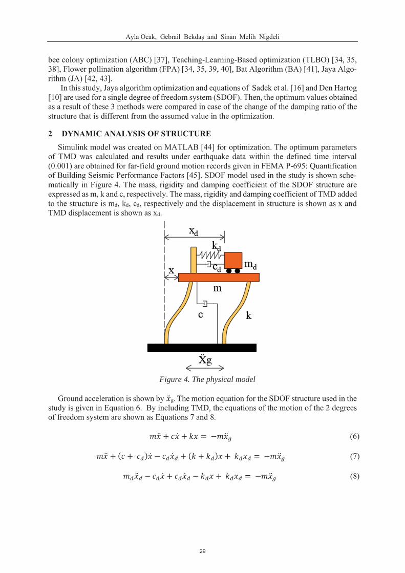
of TMD was calculated and results under earthquake data within the defined time interval (0.001) are obtained for far-field ground motion records given in FEMA P-695: Quantification of Building Seismic Performance Factors [45]. SDOF model used in the study is shown sche-matically in Figure 4. The mass, rigidity and damping coefficient of the SDOF structure are expressed as m, k and c, respectively. The mass, rigidity and damping coefficient of TMD added to the structure is md, kd, cd, respectively and the displacement in structure is shown as x and TMD displacement is shown as xd.
Figure 4. The physical model
Ground acceleration is shown by g. The motion equation for the SDOF structure used in the
study is given in Equation 6. By including TMD, the equations of the motion of the 2 degrees of freedom system are shown as Equations 7 and 8.
+ + = (6)
+ ( + ) + ( + ) + = (7) + + = (8)
29

3 THE OPTIMIZATION METHODOLOGY Using motion equations and TMD parameter calculations from the work of Den Hartog [10]
and Sadek et al. [16], the main structure and damping parameters were calculated. For the earth-quake records, which were then excited to the SDOF system, the maximum critical acceleration and displacement that will occur in the main structure were determined. The JA [45] developed by Rao, a metaheuristic algorithm inspired by victory, was selected for system optimization. With the codes prepared on the Matlab, JA was applied to optimize the system and maximum acceleration and displacements were obtained for the same earthquake records. The damping value of the SDOF structure was increased by 100 between 500-1500 Ns/m and the critical displacement and total acceleration values for all earthquake records were determined by the oprimum values of Den Hartog, Sadek et al. and JA. It has been computed and tabulated without the TMD structure and TMD structure.
The following is the equation for JA shown as Equation 9. The process of optimization based on a random assignment using the best and worst solution for the objective function obtained from Rao's work [45].
, = , + , ( , ) (9)
Xbest and Xworst used to obtain new solutions are the best solution and worst solution, respec-tively. The expression that randomly assigns between 0 and 1 is written as r1 and r2. The newly founded result for the ith solution (Xnew,i) is obtained via the existing one shown as Xold,i. The process of generating optimized new solutions and deriving existing solutions is continued for the number of iterations.
4 THE OPTIMUM RESULTS For the investigation, the parameters of the SDOF structure are taken as 1000 kg, 120000
N/m and 1000 Ns/m for m, k, and c, respectively. By using these parameters, the optimum results for a 5% mass of TMD are given in Table 1 for different approaches.
Table 1: The optimum results.
Method Den Hartog [10] Sadek et al. [16] JA (kg) 50 50 50
(Ns/m) 139.4143 270.2948 79.4850 (N/m) 5442.1769 5334.3060 7467.6313
5 DISCUSSION AND CONCLUSIONS The investigation was done by taking 5% less and more of the assumed damping valur with
100 Ns/m intervals. The displacement and acceleration maximum values are reported in Table 2 for the critical excitation with the most effect on the structure. This record is the MUL279 record of the 1994 Northridge earthquake.
As seen from Table 2, the displacement values are reduced by 30.3%, 37.4% and 42.5% for the methods of Sadek et al., Den Hartog and JA, respectively. The reduction percentages for the acceleration are 32%, 37.7% and 48.6% for Sadek et al., Den Hartog and JA, respectively. It is seen that the best method is the use of optimization algorithms like JA.
30

Table 2: The responses for different damping coefficient values.
c (Ns/m)
Without TMD With TMD
Sadek et. al. [16] Den Hartog [10] JA x (m) x (m/s2) x (m) x (m/s2) x (m) x (m/s2) x (m) x (m/s2)
500 0.2305 27.6931 0.1486 17.3602 0.1288 15.5914 0.1281 13.4663 600 0.2177 26.1615 0.1425 16.6482 0.1240 15.0228 0.1211 12.8844 700 0.2058 24.7464 0.1370 16.0236 0.1199 14.4949 0.1150 12.3404 800 0.1948 23.4298 0.1321 15.4692 0.1166 13.9941 0.1102 11.8342 900 0.1846 22.2273 0.1275 14.9393 0.1135 13.5810 0.1056 11.3630 1000 0.1765 21.2588 0.1231 14.4474 0.1105 13.2404 0.1014 10.9210 1100 0.1688 20.3615 0.1190 13.9781 0.1076 12.9108 0.0990 10.6213 1200 0.1616 19.5112 0.1151 13.5300 0.1049 12.5975 0.0968 10.3847 1300 0.1549 18.7241 0.1114 13.1140 0.1023 12.3001 0.0946 10.1603 1400 0.1487 17.9807 0.1079 12.7154 0.0998 12.0122 0.0926 9.9429 1500 0.1427 17.2813 0.1045 12.3343 0.0973 11.7334 0.0906 9.7322
For the damping values less than the assumed value, the performance of the TMD increases. For example, a 51.4% reduction occurs for the acceleration, when c value is the minimum by using JA. The opposite can be said for the increasing damping values. By this conclusion, it is seen that TMDs are more effective for the system with low inherent damping. Also, TMDs are effective when the damping coefficient value is different from the assumed one.
REFERENCES
[1] Frahm H. Device for damping of bodies. U.S. Patent No: 989,958, 1911. [2] Ormondroyd, J. and Den Hartog, J.P., 1928. The theory of the dynamic vibration absorbs.
Trans., ASME, Applied Mechanics, 50, 9-22 [3] McNamara, R.J., 1977. Tuned mass dampers for buildings. Journal of the Division,
103(9), 1785-1798. [4] Vickery, B.J., Isyumov, N. and Davenport, A.G., 1983. The role of dumping, mass and
acceleration. J. Wind Eng. Ind. Aerodyn., 11(1-3), 285-294. [5] Rana, R. and Soong, T. T., 1998. Parametric study and simplified design of tuned mass
dampers. Engineering structures, 20(3), 193-204. [6] Maurer AG, Vibration Control of Tall Buildings: Maurer Tuned Mass Dampers. [7] International Database and Gallery of Structures, https://structurae.net/en/products-ser-
vices/400-ton-pendulum-in-the-onion [8] Council on Tall Buildings and Urban Habitat, https://www.skyscrapercenter.com/build-
ing/socar-tower/2606
[9] Atlas Obscura, https://www.atlasobscura.com/places/alphabetic-tower [10] Den Hartog, J.P., 1947. Mechanical Vibrations. McGraw-Hill, New City. [11] Bishop, R.E.D. and Welbourn, D.B., 1952. The problem of the dynamic vibration ab-
sorber. Engineering, London, 174 and 769.
31

[12] Snowdon, J.C., 1959. Steady-state behavior of the dynamic absorber. Journal of the Acoustical Society of America, 31, 10961103.
[13] Falcon, K.C., Stone, B.J., Simcock, W.D. and Andrew, C., 1967. Optimization of vibra-tion absorbers: a graphical method for use on idealized systems with restricted dumping. Journal Mechanical Engineering Science. 9, 374381.
[14] Ioi, T. and Ikeda, K., 1978. On the dynamic vibration damped absorber of the vibration system. Bullet in the JSME 21, 6471.
[15] Warburton, G.B., 1982. Optimum absorber parameters for various combinations of re-sponse and excitation parameters, Earthquake Engineering and Structural Dynamics, 10, 381401.
[16] , R.M., 1997. A method of estimating the parameters of tuned mass dampers for seismic applications, Earthquake Engineering and Structural Dynamics, 26, 617635.
[17] Comeon, M.N.S. and Arfiadi, Y., 1998. Optimum design of absorber for MDOF struc-tures. Journal of Structural Engineering-ASCE, 124, 12721280.
[18] Marano, G.C., Greco, R. and Chiaia, B., 2010, A comparison between different optimi-zation criteria for tuned mass dampers design. Journal of Sound and Vibration,329, 4880-4890.
[19] Singh, M.P., Singh, S. and Moreschi, L.M., 2002. Tuned mass dampers for response con-trol of torsional buildings, Earthquake Engineering and Structural Dynamics, 31, 749769.
[20] Desu, N.B., Deb, S.K., Dutta, A., 2006. Coupled tuned mass dampers for control of cou-pled vibrations in asymmetric buildings, Struct Control Hlth., 13, 897916.
[21] Pourzeynali, S., Lavasani, H.H., Modarayi, A.H., 2007. Active control of highrise build-ing structures using fuzzy logic and genetic algorithms, Eng. Struct, 29, 446-357.
[22] Zhan, W., Cui, Y., Feng, Z., Cheung, K.C., Lam, J. and Gao, H., 2013. Joint optimization approach to building vibration control via multiple active tuned mass dampers. Mecha-tronics, 23(3), 355-368.
[23] Mohebbi, M. and Joghataie, A., 2012. Designing optimal tuned mass dampers for non-linear frames by distributed genetic algorithms. The structural Design of Tall and Special Buildings, 21(1), 57-76.
[24] Mohebbi, M., Shakeri,K., Ghanbarpout,Y. and Majzoub,H., 2013. Designing optimal multiple tuned mass dampers using genetic algorithms (Gas) for mitigating the seismic response of structures. Journal of Vibration and Control, 19(4), 605-625.
[25] Xiang, P. and Nishitani, A., 2015. Optimum design of tuned mass damper floor system integrated into bending-shear type building based on H criteria. Structural Control and Health Monitoring, 22(6), 919-938.
[26] Liu, Y., Wang, K., Mercan, O., Chen, H. and Tan, P., 2020. Experimental and numerical studies on the optimal design of tuned mass dampers for vibration control of high-rise structures. Engineering Structures, 211, 110486.
[27] Steinbuch, R., 2011. Bionic optimization of the earthquake resistance of high buildings by tuned mass dampers. Journal of Bionic Engineering, 8, 335-344.
32
[28] Farshidianfar, A., Soheili, S., 2013. Ant colony optimization of tuned mass dampers for earthquake oscillations of high-rise structures including soil structure interaction, Sile Dynamic Earthquake Eng., 51, 14-22.
[29] Leung, A.Y.T., Zhang, H., Cheng, C.C. and Lee, Y.Y., 2008. Particle optimization of TMD by non-stationary base excitation during earthquake, Earthquake Engineering and Structural Dynamics, 37, 1223-1246.
[30] Leung, A.Y.T. and Zhang, H., 2009. Particle swarm optimization of tuned mass dampers, Engineering Structures, 31, 715-728.
[31] Bekdas, G. and Nigdeli, S.M., 2017. Metaheuristic-based optimization of tuned mass dampers under earthquake excitation by considering soil-structure interaction, Soil Dy-namics and Earthquake Engineering, 92, 443-461.
[32] Nigdeli, S.M. and Bekdas,G., 2017. Optimum tuned mass damper design in the frequency domain for structures, KSCE Journal of Civil Engineering, 21(3), 912-922.
[33] Zhang, H. and Zhang, L.J., 2017. Tuned mass damper system of high-rise in take towers optimized by improved harmony search algorithm, Engineering Structures, 138, 270-282.
[34] Nigdeli, S.M., Bekdas, G. and Aydin, A., 3-7 May 2017. Metaheuristic-based optimiza-tion of tuned mass dampers on a single degree of freedom structures subjected to near-fault vibrations, 3rd International Conference on Engineering and Natural Sciences (ICENS 2017), Budapest, Hungary.
[35] Bekdas, G., Nigdeli, S.M. and Aydin, A., 8-10 May 2017. Optimization of Tuned Mass Damper for Multi-Storey Structures by using Impulsive Motions, 2nd International Con-ference on Civil and Environmental Engineering (ICOCEE 2017), Cappadocia, Turkey.
[36] Bekdas, G. and Nigdeli, S.M., 2013. Optimization of tuned mass damper with harmony search. Metaheuristic Applications in Structures and Infrastructures, 345-371.
[37] Farshidianfar, A. Soheili, S., 2013. ABC optimization of TMD parameters for tall build-ings with soil structure interaction, Interact Multiscale Mech, 6, 339-356.
[38] Nigdeli, S.M. and Bekdas,G., 2015. Teaching-Learning-Based Optimization for Estimat-ing Tuned Mass Damper Parameters, 3rd International Conference on Optimization Tech-niques in Engineering (OTENG' 15), 7-9 November, Rome, Italy.
[39] Nigdeli, S.M., Bekdas, G. and Yang, X-S, 2017. Optimum Tuning of Mass Dampers by Using a Hybrid Method Using Harmony Search and Flower Pollination Algorithm In: Harmony Search Algorithm Advances in Intelligent Systems and Computing, vol 514, Del Ser J. (eds) Springer, pp. 222-231.
[40] tuned mass damper parameters via machine learning. Journal of Building Engineering, 26, 100847.
[41] Bekdas, G., Nigdeli, S.M. and Yang, X-S., 2018. A novel bat algorithm based optimum tuning of mass dampers for improving the seismic safety of structures, Engineering Struc-tures 2018, 159:89-98.
[42] Bekdas, G., Kayabekir, A.E., Nigdeli, S.M. and Toklu, Y.C., 2019. Transfer Function Amplitude Minimization for Structures with Tuned Mass Dampers Considering Soil-Structure Interaction, Soil Dynamics and Earthquake Engineering, 116: 552-562.
33

[43] Bekdas, G., Ulusoy, S. and Nigdeli, S.M., 2018. Optimum Tuning of Mass Dampers by Impulsive Motions and Several Metaheuristic Methods 3rd International Conference on Civil and Environmental Engineering (ICOCEE), 24-27 April 2018, Izmir, Turkey.
[44] Mathworks, MATLAB, 1992. The Mathworks Inc, Natick, MA.
[45] FEMA P-695. Quantification of Building Seismic Performance Factors. Washington. [46] Rao, R., 2016. Jaya: a simple and new optimization algorithm for solving constrained and
unconstrained optimization problems, International Journal of industrial engineering computations, 7(1), 19-34.
34
A NEW MODIFIED JAYA ALGORITHM FOR OPTIMUM DESIGN OF TUNED MASS DAMPERS
Sinan Melih Nigdeli1 and 1
1 Department of Civil Engineering, Istanbul University -
e-mail: [email protected], [email protected]
Abstract
Jaya algorithm (JA) is a metaheuristic algorithm that is very simple to use because of its sim-ple features. One of these simple features is the use of a single phase of optimization. Second-ly, by the advantage of existing of a single-phase, it is a parameter-free algorithm since a switch probability is not needed to select the optimization phase. However, it is a single-phase algorithm, it uses both existing best and worst solutions in the update of candidate solutions. In the first version of JA, the best and worst solutions are considered with the same weight by multiplying with random numbers. In this study, a modified JA is proposed to include the con-sideration of different weights for best and worst solutions. To not to be dependent on the pa-rameters and to avoid always decreasing or increasing weight coefficients for the solutions, it is adjusted with a sine wave function that is updated via the iteration number. By this modifi-cation, it is possible to consider an active weight coefficient for both factors. The modified JA using sine wave is applied to the tuned mass damper (TMD) optimization problem that reduc-es the displacement of structures subjected to earthquake excitations. In the optimization pro-cess, the stroke limitation of TMD is also considered and the optimization is done for a wide set of earthquake records. The results of the proposed since wave Jaya (SJA) and JA are compared in means of convergence to the optimum results.
Keywords: Structural Optimization, Jaya Algorithm, Optimization, Metaheuristic Algo-rithms, Tuned Mass Damper
EUROGEN 2021 14th ECCOMAS Thematic Conference on
Evolutionary and Deterministic Methods for Design, Optimization and Control N. Gauger, K. Giannakoglou, M. Papadrakakis, J. Periaux (eds.)
Streamed from Athens, Greece, – 2021
35
Sinan Melih Nigdeli, and
1 INTRODUCTION Jaya Algorithm (JA) is a metaheuristic algorithm that was first presented by Rao [1] as a
single-phase algorithm that is different from the other algorithm generally having two optimi-zation phases. Like the previously developed Teaching-learning-based optimization by Rao et al. [2], it is also a user-defined parameter-free algorithm, but only a phase is used instead of two phases such as teaching and learning phases of TLBO. Although JA has a single phase, both existing best and worst solutions are used together to provide convergence to the best solution, while it diverges from the worst one.
JA has been applied to many structural optimization problems by using several modifica-tions. Kayabekir et al. [3] employed JA in the optimization of the amount of carbon fiber-reinforced polymer (CFRP) that is used to increase the shear capacity of reinforced concrete (RC) beams. Dede [4] optimized steel grillage structures by using JA that minimize the weight of the structure constrained based on LRFD-AISC. Dinh-Cong et al. [5] used JA for damage assessment in plate-like structures. Degertekin et al. [6] developed a JA-based opti-mization method for sizing, layout, and topology optimization of truss structures. Artar and Daloglu [8] optimized seismic excited steel space towers with JA. Maksym et al. [9] em-ployed JA for optimization of mass of braced dome structures with natural frequency con-straints. Khatir et al. [10] combined JA and Artificial Neural Network (ANNs) to investigate crack identification in plates. Atmaca et al. [11] used JA in the optimization of a single pylon cable-stayed bridge that has cable size and pre-stressing force as design variables. Öztürk et al. [12] optimized RC counterfort retaining walls by using JA and TLBO. Kaveh et al [13] opti-mized skeletal structure with discrete variables by improving JA to escape local optima prob-lem. Degertekin et al. [14] conducted layout optimization under natural frequency constraints
maz et al. [15] optimized RC retaining walls under static and dynamic loads via JA. the
optimization of RC T-beams via JA. JA was also used in the optimization of structural control system includes tuned mass
dampers (TMDs) [17-18], active tendon control system using proportional –integral- deriva-tive (PID) controllers [19-20] and fuzzy controllers [21].
In the present study, an improved JA is presented and tested on the tuning of TMDs. The improvement is done to change the weight of best and worst solutions in the formulation of JA. A sine wave is defined to give dynamically changing weights for each iteration.
2 SINE-WAVE JAYA ALGORITHM (SJA) Jaya means victory in the Sanskrit language and it is victorious to reach the optimum value.
The equation of JA is given in Eq. (1). t 1 t * t w ti i 1 i 2 ix x r (g | x |) r (g | x |) (1)
xit represents a set of design variables for the ith individual of tth iteration. xi
t+1 is found via using best (g*) and worst (gw) solutions. Two random numbers are represented via r1 and r2.
In the classical form of JA, g* and gw have the weight, but it is multiplied with a number. Also, the weights are always the same for all iterations. For that reason, a sine-wave function is applied for the weights of best and worst solutions. After the modification, the equation of the proposed SJA is given in Eq. (2). The sine values must be calculated as radian.
t 1 t * t w ti i 1 i 2 ix x r | sin(t) | (g | x |) r (1 | sin(t) |)(g | x |) (2)
36

Sinan Melih Nigdeli, and
The flowchart of the optimization process is summarized in Fig. 1. The design constants, design variables, objective function and design constraints are given in Section 3. The re-sponse of structure was found via dynamic analysis in the time-domain in all iterations.
Enter design constants and ranges of design variables
Are all iterations complete?
STOP
NO
Generate new solutions according to Jaya algorithm rules and calculate objective functions of the new solutions
Replace the old solutions with new ones
START
Generate initial solution matrix, calculate objective function considering design constraints
YES
Are new solutions better than old ones?
YES
NO
Figure 1: The flowchart of the optimization.
37

Sinan Melih Nigdeli, and
3 NUMERICAL EXAMPLES The design constants and the ranges of design variables are given in Table 1 for a 10-story
shear building [23]. The structure was subjected to 44 ground motions that are defined as far-field ground motions in FEMA P-695: Quantification of Building Seismic Performance Fac-tors [24].
Table 1: The design constants and variables
Type Symbol Definition Value Constant mi Mass of ith story 360 t
ki Stiffness of ith story 650 MN/m ci Damping coefficient of ith story 6.2 MNs/m md Mass of TMD 180 t
Variable Td Period of TMD 0.5s-1.5s d Damping ratio of TMD 1%-50%
The objective function of the problem is the minimization of top story displacement (x10) of the structure as seen in Eq. (3). It is obtained by solving the equation of motion (Eq. (4)) that includes mass (M), stiffness (K), damping (C) matrices, a vector ones ({1}) and ground acceleration gx . x(t) defines the response of the structure.
10f (x) minimize(| x |) (3)
gMx(t) Cx(t) Kx(t) M 1 x (t) (4)
The optimization problem is also constrained with the function (g1) given as Eq. (5). It is a normalized stroke capacity of the TMD to limit its movement. It must be smaller than a user-defined value called stmax.
(5)
xd is the displacement of TMD with respect to the ground. The design variables are formu-lated in Eqs. (6) and (7) with respect to mass (md), stiffness (kd) and damping coefficient (cd) of TMD.
d
dd k
m2T (6)
d
dd
dd
mk
m2
c (7)
In the optimization, the classical version of JA and SJA algorithm were compared. 100 maximum number of iterations are conducted and 10 cycles of optimization are applied. stmax is taken as 1. The population number which defines the number of sets of design varia-bles is taken as 5.
38

Sinan Melih Nigdeli, and
4 RESULTS AND CONCLUSIONS The maximum displacement of the top story of the structure is 0.410109 m and it is ob-
tained under the BOL090 component of the Bolu record of 1999 Düzce, Turkey earthquake. The optimum results of JA and SJA are given in Table 2.
Table 2: The optimum results
JA SJA Td (s) 0.904560044 0.902517645
d 0.283683914 0.282289564 f(x) (best) (m) 0.320240847 0.320235126 f(x) (ave) (m) 0.323361718 0.322733436 std 0.004388982 0.003896575 iteration 38 21
According to the results, JA and SJA are both effective to reduce the maximum top story displacement by 22%. SJA has a slightly smaller objective function, but it has a significantly smaller average and standard deviation (std) value than JA. Also, it is possible to find the op-timum solution in the 21th iteration, while JA needs more iterations to reach the final value. The convergence plot for the optimization is presented in Fig. 2. Although JA has a good convergence at the start of the optimization process, SJA quickly converges to the final value.
Figure 2: The convergence plot.
REFERENCES [1] Rao, R. (2016). Jaya: A simple and new optimization algorithm for solving constrained
and unconstrained optimization problems. International Journal of Industrial Engineer-ing Computations, 7(1), 19-34.
39
Sinan Melih Nigdeli, and
[2] Rao, R. V., Savsani, V. J., & Vakharia, D. P. (2011). Teaching–learning-based optimi-zation: a novel method for constrained mechanical design optimization prob-lems. Computer-Aided Design, 43(3), 303-315.
[3] Kaybased optimum carbon fiber reinforced polymer design for reinforced concrete beams. In AIP Conference Proceedings (Vol. 1978, No. 1, p. 260006). AIP Publishing LLC.
[4] Dede, T. (2018). Jaya algorithm to solve single objective size optimization problem for steel grillage structures. Steel and Composite Structures, 26(2), 163-170.
[5] Dinh-Cong, D., Vo-Duy, T., Ho-Huu, V., & Nguyen-Thoi, T. (2019). Damage assess-ment in plate-like structures using a two-stage method based on modal strain energy change and Jaya algorithm. Inverse Problems in Science and Engineering, 27(2), 166-189.
[6] Degertekin, S. O., Lamberti, L., & Ugur, I. B. (2018). Sizing, layout and topology de-sign optimization of truss structures using the Jaya algorithm. Applied soft computing, 70, 903-928.
[7] Degertekin, S. O., Lamberti, L., & Ugur, I. B. (2019). Discrete sizing/layout/topology optimization of truss structures with an advanced Jaya algorithm. Applied Soft Compu-ting, 79, 363-390.
[8] Artar, M., & Daloglu, A. T. (2019). Optimum design of steel space truss towers under seismic effect using Jaya algorithm. Structural Engineering and Mechanics, 71(1), 1-12.
[9] Grzywinski, M., Dede, T., & Ozdemir, Y. I. (2019). Optimization of the braced dome structures by using Jaya algorithm with frequency constraints. Steel and Composite Structures, 30(1), 47-55.
[10] Khatir, S., Boutchicha, D., Le Thanh, C., Tran-Ngoc, H., Nguyen, T. N., & Abdel-Wahab, M. (2020). Improved ANN technique combined with Jaya algorithm for crack identification in plates using XIGA and experimental analysis. Theoretical and Applied Fracture Mechanics, 107, 102554.
[11] Atmaca, B., Dede, T., & Grzywinski, M. (2020). Optimization of cables size and pre-stressing force for a single pylon cable-stayed bridge with Jaya algorithm. Steel and Composite Structures, 34(6), 853-862.
[12] Öztürk, H. T., Dede, T., & Türker, E. (2020, June). Optimum design of reinforced con-crete counterfort retaining walls using TLBO, Jaya algorithm. In Structures (Vol. 25, pp. 285-296). Elsevier.
[13] Kaveh, A., Hosseini, S. M., & Zaerreza, A. (2021, February). Improved Shuffled Jaya algorithm for sizing optimization of skeletal structures with discrete variables. In Struc-tures (Vol. 29, pp. 107-128). Elsevier.
[14] Degertekin, S. O., Bayar, G. Y., & Lamberti, L. (2021). Parameter free Jaya algorithm for truss sizing-layout optimization under natural frequency constraints. Computers & Structures, 245, 106461.
[15] Optimum Design of Reinforced Concrete Retaining Walls Under Static and Dynamic Loads Using Jaya Al-gorithm. In International Conference on Harmony Search Algorithm (pp. 187-196). Springer, Singapore.
40

Sinan Melih Nigdeli, and
[16] ptimal Cost Design of Single-Story Reinforced Concrete Frames Using Jaya Algorithm. In International Conference on Harmony Search Algorithm (pp. 179-186). Springer, Singapore.
[17] , S. M. (2019). Optimum design of T-beams us-ing Jaya algorithm. In 3rd International Conference on Engineering Technology and In-novation (ICETI), Belgrad, Serbia.
[18] amplitude minimization for structures with tuned mass dampers considering soil-structure interaction. Soil Dynamics and Earthquake Engineering, 116, 552-562.
[19] Kayabekir, A. E. , G., Nigdeli, S.M. (2020). Active Tuned Mass Dampers for Control of Seismic Structures. WSEAS Transactions on Computers, 19, 122-128.
[20] Ulusoy, S., Bekdas, G., & Nigdeli, S. M. (2020). Active structural control via metaheu-ristic algorithms considering soil-structure interaction. Structural Engineering and Me-chanics, 75(2), 175-191.
[21] Ulus -based tuning of PID controllers for seismic structures and verification of robustness. Journal of Building Engineering, 33, 101647.
[22] Azizi, M., Ghasemi, S. A. M., Ejlali, R. G., & Talatahari, S. (2020). Optimum design of fuzzy controller using hybrid ant lion optimizer and Jaya algorithm. Artificial Intelli-gence Review, 53(3), 1553-1584.
[23] M.P. Singh, S. Singh, L.M. Moreschi, Tuned mass dampers for response control of tor-sional buildings, Earthq. Eng. Struct. D. 31 (2002) 749–769.
[24] FEMA P-695, Quantification of Building Seismic Performance Factors, Federal Emer-gency Management Agency, Washington DC, 2009.
41

AERODYNAMIC SHAPE OPTIMIZATION OF THE MEXICO WINDTURBINE BLADE USING THE CONTINUOUS ADJOINT METHOD
E. M. Papoutsis-Kiachagias1, M. Erfan Farhikhteh1, T. Skamagkis1, andK. C. Giannakoglou1
1National Technical University of Athens,Parallel CFD & Optimization Unit, School of Mechanical Engineering
Zografou Campus, 9 Iroon Polytechniou Stre-mail: {vpapout,mohammaderfanfarhikhteh,themistoklissk, kgianna}@mail.ntua.gr
Keywords: Aerodynamic Optimization, Continuous Adjoint, MEXICO Wind Turbine, Recur-
sive Projection Method.
Abstract. This paper presents the aerodynamic shape optimization of the MEXICO wind tur-bine (WT) blade, targeting the maximization of the axial moment and, hence, of the producedpower. The optimization is conducted using the OpenFOAM-based continuous adjoint solvernamed adjointOptimisationFoam, developed and made publicly available by the group of au-thors. This implements and solves the adjoint to the Navier-Stokes system of equations, coupledwith the differentiation of the Spalart-Allmaras turbulence model. Herein, this was extended toinclude the adjoint to the flow equations which are solved for the absolute velocity in the rela-tive reference frame. Challenges in the convergence of the adjoint equations, mostly attributedto flow unsteadiness causing marginal convergence of the steady flow solver, are treated byadditionally implementing the Recursive Projection Method (RPM). Assessment of the adjointsensitivities with finite differences in a similar 2D case is also included. Then, the flow solutionfor the MEXICO WT case is compared with the outcome of another CFD solvers and exper-imental data, prior to the application of the expanded optimization software to maximize theaxial moment of the WT. The blade and the displacement of the surrounding grid nodes areparameterized using a volumetric B-Splines morphing box. The optimization designed a bladebended in the axial direction axial moment, having a higher by 10.8%.
EUROGEN 2021 14th ECCOMAS Thematic Conference on
Evolutionary and Deterministic Methods for Design, Optimization and Control N. Gauger, K. Giannakoglou, M. Papadrakakis, J. Periaux (eds.)
Streamed from Athens, Greece, – 2021
42

E. M. Papoutsis-Kiachagias, M. Erfan Farhikhteh, T. Skamagkis, and K. C. Giannakoglou
1 INTRODUCTION
Wind energy is a widely used renewable energy source producing green and clean energy [1].
Among other, an increased interest has surfaced on how to decrease the cost of the produced
energy by wind turbines (WTs). This can be achieved by reducing the turbine capital cost
and/or by increasing the annual energy production. Upscaling WTs to have a bigger swept
area is a way to extract more energy, however, this solution affects the structural mechanics of
the WT [2], since mass increases with the cube of the rotor radius. Generally, the design of
WTs is a multidisciplinary trade-off among aerodynamic performance, structural efficiency and
manufacturing cost [3].
Currently, low-fidelity models are often used to design WT blades, because of their low com-
putational cost and simple implementation. Among them, Blade Element Momentum (BEM)
models are the most widely used [4]. Depending on the application however, such a model may
have limited success in accurately capturing viscous flow effects, compressibility and complex
3D patterns; hence, 3D Computational Fluid Dynamics (CFD) software should be used instead.
In other areas, such as aerospace or the automotive industry, CFD-based aerodynamic shape
optimization is used on a regular basis [5, 6]. Similar methods in the wind energy field are
not yet in widespread use. High-fidelity CFD-based shape optimization can be performed with
or without computing the gradient of the objective function. In [7], a WT blade winglet was
optimized using a 3D CFD model and a gradient-free method using two design variables to
increase the moment which, in turn, increased power production by 9%. Increasing the number
of design variables is expected to increase the optimization turn-around time of gradient-free
methods a lot. Gradient-based optimization may overcome this manner as the adjoint method
is the only way to compute the required gradient components at a cost that does not scale with
their number [8, 9]. The first time the adjoint to a RANS equations solver was used to optimize
the lift-to-drag ratio of a WT blade airfoil was in [10].
A few 3D adjoint-based shape optimizations considered modelling the rotation effects. In
one of them [11], the NREL Phase VI rotor was optimized using the RANS equations. The
continuous adjoint to the discrete adjoint to the RANS equations, including the adjoint to the
Spalart-Allmaras turbulence model, was used in [12] to maximize the power of the MEXICO
WT rotor with the flow and adjoint solvers running on GPUs.
In the present work, the aerodynamic shape of the MEXICO WT blade is optimized in order
to increase the axial moment and, thus, power production. The RANS equations are formulated
in the relative reference frame and solved for the absolute velocity. Initially, the CFD analysis of
the MEXICO WT blade is validated with two other CFD solvers and experimental data. A con-
tinuous adjoint formulation is then used to compute the gradient and support the optimization.
The adjoint to the terms emerging from changing the reference frame to the relative one is also
included, along with the differentiation of the Spalart-Allmaras turbulence model. Although
a steady-state RANS solver was used and was sufficient in capturing the main aspects of the
flow, small scale unsteadiness led to oscillating flow solver residuals and, as a result, the adjoint
solver diverged on most optimization cycles. To stabilize the latter and allow an uninterrupted
optimization, the Recursive Projection Method (RPM), developed in [13] for the stabilization
of unstable iterative procedures, was used to support the adjoint method, leading to an increased
axial moment by 10.8%.
43
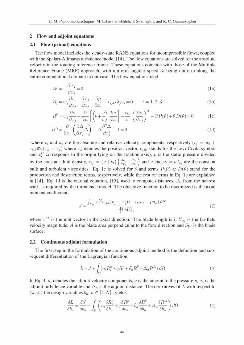
E. M. Papoutsis-Kiachagias, M. Erfan Farhikhteh, T. Skamagkis, and K. C. Giannakoglou
2 Flow and adjoint equations
2.1 Flow (primal) equations
The flow model includes the steady-state RANS equations for incompressible flows, coupled
with the Spalart-Allmaras turbulence model [14]. The flow equations are solved for the absolute
velocity in the rotating reference frame. These equations coincide with those of the Multiple
Reference Frame (MRF) approach, with uniform angular speed � being uniform along the
entire computational domain in our case. The flow equations read
Rp=−∂wj
∂xj
=0 (1a)
Rvi =wj
∂vi∂xj
− ∂τij∂xj
+∂p
∂xi
+ eijk�jvk=0 , i = 1, 2, 3 (1b)
Rν=wj∂ν
∂xj
− ∂
∂xj
[(ν+
ν
σ
)∂ν
∂xj
]− cb2
σ
(∂ν
∂xj
)2
− ν P (ν)+νD(ν)=0 (1c)
RΔ=∂
∂xj
(∂Δ
∂xj
Δ
)−Δ
∂2Δ
∂x2j
− 1=0 (1d)
where vi and wi are the absolute and relative velocity components, respectively (vi = wi +eijk�j(xk − xc
k) where xk denotes the position vector, eijk stands for the Levi-Civita symbol
and xCk corresponds to the origin lying on the rotation axis), p is the static pressure divided
by the constant fluid density, τij = (ν+νt)(
∂vi∂xj
+∂vj∂xi
)and ν and νt = νfv1 are the constant
bulk and turbulent viscosities. Eq. 1c is solved for ν and terms P (ν) & D(ν) stand for the
production and destruction terms, respectively, while the rest of terms in Eq. 1c are explained
in [14]. Eq. 1d is the eikonal equation, [15], used to compute distances, Δ, from the nearest
wall, as required by the turbulence model. The objective function to be maximized is the axial
moment coefficient,
J=
∫SW
rMi eijk(xj − xcj) (−τklnl + pnk) dS
12lAU2∞
(2)
where rMi is the unit vector in the axial direction. The blade length is l, U∞ is the far-field
velocity magnitude, A is the blade area perpendicular to the flow direction and SW is the blade
surface.
2.2 Continuous adjoint formulation
The first step in the formulation of the continuous adjoint method is the definition and sub-
sequent differentiation of the Lagrangian function
L=J+
∫Ω
(uiR
vi +qRp+νaR
ν+ΔaRΔ)dΩ (3)
In Eq. 3, ui denotes the adjoint velocity components, q is the adjoint to the pressure p, νa is the
adjoint turbulence variable and Δa is the adjoint distance. The derivatives of L with respect to
(w.r.t.) the design variables bn, n ∈ [1, N ] , yields
δL
δbn=
δJ
δbn+
∫Ω
(uiδRv
i
δbn+q
δRp
δbn+νa
δRν
δbn+Δa
δRΔ
δbn
)dΩ (4)
44

E. M. Papoutsis-Kiachagias, M. Erfan Farhikhteh, T. Skamagkis, and K. C. Giannakoglou
where δδbn
(.) represents total (or material) derivatives and
δJ
δbn=
112lAU2∞
[ ∫SW
rMi eijk(−τklnl + pnk)δxj
δbndS−
∫SW
rMi eijk(xj − xcj)δτklδbn
nldS
+
∫SW
rMi eijk(xj − xcj)(−τkl + pδlk)
δ(nldS)
δbn+
∫SW
rMi eijk(xj − xcj)
δp
δbnnkdS
](5)
Further developing Eq. 4 makes use of δδbn
(∂(.)∂xj
)= ∂
∂xj
(δ(.)δbn
)− ∂(.)
∂xk
∂∂xj
(δxk
δbn
)(see [16]), and
the Gauss divergence theorem. Only the differentiation of the continuity equation is shown∫Ω
qδRp
δbndΩ=
∫SW
−qnjδwj
δbdS
+
∫Ω
[∂q
∂xj
δvjδbn
− ∂q
∂xj
ejlk�lδxk
δbn+q
∂vj∂xk
∂
∂xj
(δxk
δbn
)−qejlk�l
∂
∂xj
(δxk
δbn
)]dΩ
(6)
In Eq. 6, all terms including the so-called grid sensitivities δxk
δbncontribute to the sensitivity
derivatives. The rest of integrals in Eq. 3 are expanded similary. Boundary integrals including
flow variations contribute to the adjoint boundary conditions whereas field integrals of the same
quantities contribute to the field adjoint equations.
2.2.1 Field adjoint equations
In order to avoid the computation of variations in the flow variables w.r.t. bn within the field
integrals of the developed form of Eq. 4, the multipliers of these terms are set to zero. Thus, the
field adjoint equations
Rq=−∂uj
∂xj
= 0 (7a)
Rui =uj
∂vj∂xi
− ∂(wjui)
∂xj
−∂τaij∂xj
+∂q
∂xi
+eijkuj�k+νa∂ν
∂xi
− ∂
∂xl
(νaν
CYY
emjk∂vk∂xj
emli
)=0 , i=1, 2, 3 (7b)
Rνa =−∂(wj νa)
∂xj
− ∂
∂xj
[(ν+
ν
σ
)∂νa∂xj
]+1
σ
∂νa∂xj
∂ν
∂xj
+2cb2σ
∂
∂xj
(νa
∂ν
∂xj
)+νaνCν+
∂νt∂ν
∂ui
∂xj
(∂vi∂xj
+∂vj∂xi
)+(−P+D) νa=0 (7c)
RΔa =−2∂
∂xj
(Δa
∂Δ
∂xj
)+ννaCΔ=0 (7d)
45

E. M. Papoutsis-Kiachagias, M. Erfan Farhikhteh, T. Skamagkis, and K. C. Giannakoglou
emerge, where τaij = (ν+νt)(
∂ui
∂xj+
∂uj
∂xi
)is the adjoint stress tensor. The Cνa , CY and CΔ terms
in Eq. 7c are defined in [17].
2.3 Sensitivity derivatives
After eliminating all other integrals in the developed form of Eq. 4, by satisfying the adjoint
field equations and boundary conditions (omitted here in the interest of space; see [9] for a
detailed derivation), the remaining terms can be computed at a negligible cost and constitute the
sensitivity derivatives of J , which read
δL
δbn=
∫SW
τaijnjeikl�kδxl
δbndS+
112lAU2∞
[ ∫SW
rMi eijk(−τklnl + pnk)δxj
δbndS
−∫SW
rMi eijk(xj − xcj)(τkl + pδlk)
δ(nldS)
δbn
]−∫Ω
(∂q
∂xj
+ ui∂vi∂xj
+ νa∂ν
∂xj
)ejlk�l
δxk
δbndΩ
−∫Ω
[q∂vj∂xk
+ qejlk�l + uiwj∂vi∂xj
+ τaij∂vi∂xk
+ uj∂p
∂xk
+νawj∂ν
∂xk
+
(ν+
ν
σ
)∂νa∂xj
∂ν
∂xk
−2νacb2σ
∂ν
∂xj
∂ν
∂xk
+ νaνCYYq
‖�Y ‖eqjl
∂vl∂xk
+2Δa∂Δ
∂xj
∂Δ
∂xk
]∂
∂xj
(δxk
δbn
)dΩ (8)
where �Y is the flow vorticity.
3 The Recursive Projection Method
Both the primal and adjoint equations are solved in OpenFOAM using a pressure-based
solver. The primal and adjoint solvers are both variants of the standard SIMPLE algorithm [18]
with small modifications. The slow convergence, or even divergence, of SIMPLE-like solvers
is usually related to a difficulty in reducing the primal/adjoint pressure equation residuals. This
difficulty is even more pronounced in cases that exhibit unsteadiness where it is not unusual
for the steady primal solver residuals to marginally converge and then begin to oscillate after a
number of iterations. This is usually accompanied by the subsequent divergence of the contin-
uous adjoint solver; this behavior may be observed even in cases with small-scale unsteadiness
[19]. This issue was observed in the optimisation of the WT and, on a number of optimization
cycles, the use of the RPM was necessary to make the adjoint equations converge.
The RPM is a technique for stabilizing unstable iterative procedures, formally written as
UUU (n+1) = FFF (UUU (n)), where UUU ∈ RM is the array of (primal or adjoint) unknowns and n the
iteration counter. If the largest eigenvalue of the Jacobian matrix FU exceeds unity, such a
scheme is expected to diverge and, on many occasions, the RPM can make such an otherwise
diverging scheme converge. First, the method needs to identify the diverging modes of FU , i.e.
the eigenvectors corresponding to the largest eigenvalues. Once identified, and assuming that
these modes are m in total, they can form a basis Z∈RM×m which is used to split the solution
space RM into two parts: the unstable subspace P∈RM , spanned by the m diverging modes of
FU , and its orthogonal complement Q∈RM . The solution UUU is also decomposed into Up ∈ P
and Uq ∈ Q; the unstable and stable parts of the solution respectively. A stabilized iterative
scheme is thus derived where a Newton iteration is performed on Up while the original scheme
is retained for Uq. This way, the RPM makes a previously diverging scheme converge.
Practically, m is initially zero and gradually grows as diverging and slowly decaying modes
are identified and incrementally appended to Z throughout the solution of the adjoint equations.
46

E. M. Papoutsis-Kiachagias, M. Erfan Farhikhteh, T. Skamagkis, and K. C. Giannakoglou
Additionally, Z is approximated using power iterations on an initial matrix estimate (more
details about the implementation of the RPM can be found in [13]). Finally, the new scheme
derived through the RPM becomes stable after all the diverging modes have been identified and
provided that Z has been approximated with sufficient accuracy.
4 Analysis and Optimization of the WT blades
This work presents the aerodynamic shape optimization of a Horizontal Axis Wind Turbine
(HAWT) blade, namely that of the MEXICO WT, associated with the EU project ”Model Rotor
Experiments In Controlled Conditions” [20]. Measurements were performed in the Large Low-
Speed Facility of DNW in the Netherlands [20, 21]. The computational domain Ω includes
one third of the WT disk, with periodic boundary conditions. The CFD domain and mesh are
presented in Fig. 1. The hybrid CFD mesh is generated with ≈ 107 cells using Pointwise.
Figure 1: CFD domain and mesh around the MEXICO WT blade.
4.1 Flow Solver Verification
The wind speed and yaw angle are 10m/s and 0◦, respectively. The pressure coefficient
distribution on a number of different spanwise positions over the blade is shown in Fig. 2.
OpenFOAM-based results are compared with wind tunnel measurements and two other CFD
results. The latter are obtained from the MaPFlow code of the Lab. of Aerodynamics, NTUA
[22] and the GPU-enabled PUMA code (incompressible flow solver) of the Parallel CFD &
Optimization Unit, NTUA [12]. All CFD results are in very good agreement.
47

E. M. Papoutsis-Kiachagias, M. Erfan Farhikhteh, T. Skamagkis, and K. C. Giannakoglou
-2
-1.5
-1
-0.5
0
0.5
1
1.5 0 0.2 0.4 0.6 0.8 1
Cp
x/c
OpenFOAMExperimental
PUMAMaPFlow
(a) 25% Span
-1.5
-1
-0.5
0
0.5
1
1.5 0 0.2 0.4 0.6 0.8 1
Cp
x/c
OpenFOAMExperimental
PUMAMaPFlow
(b) 35% Span
-2
-1.5
-1
-0.5
0
0.5
1
1.5 0 0.2 0.4 0.6 0.8 1
Cp
x/c
OpenFOAMExperimental
PUMAMaPFlow
(c) 60% Span
-1.5
-1
-0.5
0
0.5
1
1.5 0 0.2 0.4 0.6 0.8 1
Cp
x/c
OpenFOAMExperimental
PUMAMaPFlow
(d) 82% Span
Figure 2: MEXICO WT Blade: Comparison of the pressure coefficient computed by Open-
FOAM, PUMA and MaPFlow with measurements, at four spanwise positions.
It can be observed that pressure on the suction side is underpredicted by all CFD results
and, in those cases, the experimental results are not in good agreement with CFD. A number of
possible reasons for this are mentioned in [23]. On the other hand, all CFD results shown here
and additional ones presented in [23] are in very good agreement.
4.2 Verification of the Sensitivity Derivatives
The adjoint-based sensitivity derivatives are verified against the results of finite-differences
(FDs) in this section. Since FDs are very time consuming due to the need to solve the flow
48

E. M. Papoutsis-Kiachagias, M. Erfan Farhikhteh, T. Skamagkis, and K. C. Giannakoglou
equations twice for each design variable, the adjoint-based sensitivity derivatives are verified
on a 2D mixer case, Fig. 3. Adjoint-based sensitivities are in a good agreement with FDs and
can be used in a gradient-based optimization loop.
(a)
-0.00015
-0.0001
-5e-05
0
5e-05
0.0001
0.00015
40 45 50 55 60 65
dJ/d
b x
Control Point
adjointFD
(b)
-0.00015
-0.0001
-5e-05
0
5e-05
0.0001
0.00015
40 45 50 55 60 65
dJ/d
b y
Control Point
adjointFD
(c)
Figure 3: 2D mixer: Verification of the adjoint-based sensitivity derivatives with FDs. (a)
Case geometry; blue/red lines correspond to rotating/stationary walls. The grey area indicates
the rotating part of the computational domain, i.e. the part in which additional terms in the
momentum equations, Eq. 1b are introduced. The lattice of control points parameterizing the
rotor is also shown. The coordinates of the control points in red act as the design variables.
(b)-(c) Comparison of the adjoint-based derivatives with FDs for the x and y coordinates of the
control points.
4.3 Wind Turbine Blade Optimization
After validating the flow solver and sensitivity derivatives, the next step includes the opti-
mization of the WT blade to maximize the axial moment coefficient, Eq. 2. The blade was
parameterized using the volumetric B-Splines morphing box presented in Fig. 4. The role un-
dertaken by the RPM within the first optimization cycle is explained in Fig. 5. With a converged
adjoint, optimization ensued and, after 15 cycles, the axial moment coefficient has increased by
10.8%, from 0.2332 to 0.2584.
49

E. M. Papoutsis-Kiachagias, M. Erfan Farhikhteh, T. Skamagkis, and K. C. Giannakoglou
Figure 4: MEXICO WT Blade: A 6×12×6 volumetric B-Splines morphing box parameterizes
the blade and part of the mesh. Control points (CPs) in red were allowed to move only in the
axial direction (z); CPs in blue remain frozen during the optimization.
1
10-6
10-4
10-2
102
104
0 10000 20000 30000
Res
idua
ls
No. Iterations
With RPMWithout RPM
Figure 5: MEXICO WT Blade: Convergence of the adjoint equations with/without the RPM
(blue/red) within the first optimization cycle. Residuals averaged over the ensemble of equations
are plotted in logarithmic scale.
From Figs. 6, it can be observed that the optimizer has mainly changed the shape of the blade
close to its tip. Smaller changes can also be seen close to the root. Fig. 7 demonstrates that the
optimizer bended the tip towards the axial flow direction and slightly increased the blade yaw
angle at the same position.
50

E. M. Papoutsis-Kiachagias, M. Erfan Farhikhteh, T. Skamagkis, and K. C. Giannakoglou
(a) 25% Span (b) 35% Span
(c) 60% Span (d) 82% Span
Figure 6: Comparison of the baseline (magenta) and optimized (green) blade sections at a
number of spanwise positions.
Figure 7: Comparison of the baseline (white) and optimized (green) geometries of the blade, as
seen from its tip.
To get a clearer view on local deformations along the blade span, the cumulative normal dis-
placement of the optimized blade surface is presented in Figs. 8.
(a) Pressure side
(b) Suction side
Figure 8: Cumulative normal displacements of the blade surface. Positive/negative signs
(red/blue) indicate inward/outward displacements.
51

E. M. Papoutsis-Kiachagias, M. Erfan Farhikhteh, T. Skamagkis, and K. C. Giannakoglou
The comparison of the pressure coefficient distribution on the blade for the baseline and
optimized geometries is presented in Figs. 9 and 10 for the pressure and suction sides, respec-
tively. Figs. 10a and 10b demonstrate that the largest pressure coefficient difference is at the
middle and upper part of the blade, whereas the pressure coefficient at the leading and trailing
edges does not change significantly w.r.t. the baseline design. For the pressure side of the blade,
Fig. 9a and 9b show that the significant pressure coefficient difference happens at the upper part
of the blade.
(a) Baseline
(b) Optimized
Figure 9: Comparison of the pressure coefficient distribution on the blade pressure side.
(a) Baseline
(b) Optimized
Figure 10: Comparison of the pressure coefficient distribution on the blade suction side.
The pressure coefficient distributions of the baseline and optimized geometries are also plot-
ted in Fig. 11 at a number of spanwise positions. It is evident that the largest increase in the
objective function comes from the tip, whereas the pressure coefficient is almost unchanged
close to its root.
52

E. M. Papoutsis-Kiachagias, M. Erfan Farhikhteh, T. Skamagkis, and K. C. Giannakoglou
-2
-1.5
-1
-0.5
0
0.5
1
1.5 0 0.2 0.4 0.6 0.8 1
Cp
x/c
BaselineOptimized
(a) 25% Span
-1.5
-1
-0.5
0
0.5
1
1.5 0 0.2 0.4 0.6 0.8 1
Cp
x/c
BaselineOptimized
(b) 35% Span
-2
-1.5
-1
-0.5
0
0.5
1
1.5 0 0.2 0.4 0.6 0.8 1
Cp
x/c
BaselineOptimized
(c) 60% Span
-1.5
-1
-0.5
0
0.5
1
1.5 0 0.2 0.4 0.6 0.8 1
Cp
x/c
BaselineOptimized
(d) 82% Span
Figure 11: Comparison of the pressure coefficient of the baseline and optimized blades at four
spanwise positions.
5 Conclusions
This paper presented an application of the publicly available adjointOptimisationFoam,
the adjoint-based optimizer within OpenFOAM developed by the authors, to the optimization of
the MEXICO wind turbine, targeting an increased axial moment coefficient. The capabilities of
the software were enhanced by including the adjoint to the terms taking the rotation of the com-
putational domain into consideration. Convergence difficulties, encountered in the numerical
solution of the adjoint equations, were treated using the RPM which enabled the adjoint solver
to converge and compute the required sensitivities. The application of the extended software
led to an increase in the axial moment coefficient by 10.8%, by mainly bending the blade tip in
the axial direction and changing the blade yaw angle close to the tip.
6 Acknowledgments
This project has received funding from the European Union’s Horizon 2020 research and inno-
vation program under the Marie Sklodowska Curie Grant Agreement No 860101 (zEPHYR).
53

E. M. Papoutsis-Kiachagias, M. Erfan Farhikhteh, T. Skamagkis, and K. C. Giannakoglou
REFERENCES
[1] T. Liu, P.J. Tavner, Y. Feng, and Y.N. Qiu. Review of recent offshore wind power devel-
opments in China. Wind Energy, 16(5):786–803, 2013.
[2] T. Ashuri and MB. Zaayer. Size effect on wind turbine blade’s design drivers. In Proceed-ings of the European Wind Energy Conference and Exhibition EWEC, Brussels, 2008.
[3] J.R.R.A. Martins and A.B. Lambe. Multidisciplinary design optimization: A survey of
architectures. AIAA Journal, 51(9):2049–2075, 2013.
[4] H. Glauert. The elements of aerofoil and airscrew theory. Cambridge University Press,
1983.
[5] S. Chen, Z. Lyu, G.K.W. Kenway, and J.R.R.A. Martins. Aerodynamic shape optimization
of common research model wing–body–tail configuration. Journal of Aircraft, 53(1):276–
293, 2016.
[6] E.M. Papoutsis-Kiachagias, V.G. Asouti, K.C. Giannakoglou, K. Gkagkas, S. Shimokawa,
and E. Itakura. Multi-point aerodynamic shape optimization of cars based on continuous
adjoint. Structural and Multidisciplinary Optimization, 59(2):675–694, 2019.
[7] M.A. Elfarra, N. Sezer-Uzol, and I.S. Akmandor. NREL VI rotor blade: Numerical inves-
tigation and winglet design and optimization using CFD. Wind Energy, 17(4):605–626,
2014.
[8] J.E.V. Peter and R.P. Dwight. Numerical sensitivity analysis for aerodynamic optimiza-
tion: A survey of approaches. Computers & Fluids, 39(3):373–391, 2010.
[9] E.M. Papoutsis-Kiachagias and K.C. Giannakoglou. Continuous adjoint methods for tur-
bulent flows, applied to shape and topology optimization: industrial applications. Archivesof Computational Methods in Engineering, 23(2):255–299, 2016.
[10] R. Ritlop and S. Nadarajah. Design of wind turbine profiles via a preconditioned adjoint-
based aerodynamic shape optimization. 47th AIAA Aerospace Sciences Meeting includingThe New Horizons Forum and Aerospace Exposition, pages 2009–1547, 2009.
[11] T. Dhert, T. Ashuri, and J.R.R.A. Martins. Aerodynamic shape optimization of wind
turbine blades using a reynolds-averaged Navier–Stokes model and an adjoint method.
Wind Energy, 20(5):909–926, 2017.
[12] K.T. Tsiakas, X.S. Trompoukis, V. Asouti, and K.C. Giannakoglou. Shape optimization
of wind turbine blades using the continuous adjoint method and volumetric NURBS on a
GPU cluster. In Advances in Evolutionary and Deterministic Methods for Design, Opti-mization and Control in Engineering and Sciences, pages 131–144. Springer, 2019.
[13] G.M. Shroff and H. Keller. Stabilization of unstable procedures: The Recursive Projection
Method. SIAM Journal of Numerical Analysis, 30(4):1099–1120, 1993.
[14] P. Spalart and S. Allmaras. A one-equation turbulence model for aerodynamic flows. AIAAPaper No. 92-0439, 1992.
54

E. M. Papoutsis-Kiachagias, M. Erfan Farhikhteh, T. Skamagkis, and K. C. Giannakoglou
[15] P. Tucker. Differential equation-based wall distance computation for DES and RANS.
Journal of Computational Physics, 190:229–248, 2003.
[16] D. Papadimitriou and K. Giannakoglou. A continuous adjoint method with objective func-
tion derivatives based on boundary integrals for inviscid and viscous flow. Computers &Fluids, 36(2):325–341, 2007.
[17] A.S. Zymaris, D.I. Papadimitriou, K.C. Giannakoglou, and C. Othmer. Continuous adjoint
approach to the Spalart-Allmaras turbulence model for incompressible flows. Computers& Fluids, 38(8):1528–1538, 2009.
[18] S. Patankar. Numerical Heat Transfer and Fluid Flow. Hemisphere, Taylor & Francis
Group, 1st edition, 1980.
[19] R. Dwight and D. Vollmer. Efficient algorithms for solution of the adjoint compressible
Navier-Stokes equations with applications. In Proceedings of the ONERA-DLR AerospaceSymposium (ODAS), Toulouse, 2006.
[20] J.G. Schepers and H. Snel. Model experiments in controlled conditions. Technical Report
E-07-042, Energy Research Center of the Netherlands, 2007.
[21] H. Snel, J.G. Schepers, and L. Pascal. First results from mexnext: Analysis of detailed
aerodynamic measurements on a 4.5 diameter rotor placed in the large German Dutch
Wind Tunnel DNW. In European Wind Energy Conference and Exhibition (EWEC), War-
saw, Poland, 2010.
[22] G. Papadakis, S. Voutsinas, G. Sieros, and T. Chaviaropoulos. CFD aerodynamic anal-
ysis of non-conventional airfoil sections for very large rotor blades. Journal of Physics:Conference Series, 555 012104, 2014.
[23] J.G. Schepers, K. Boorsma, T. Cho, S. Gomez-Iradi, P. Schaffarczyk, WZ. Shen, T. Lutz,
B. Stoevesandt, S. Schreck, D. Micallef, et al. Analysis of MEXICO wind tunnel mea-
surements. Final report of IEA task 29, Mexnext (phase 1). Technical Report E-12-004,
ECN, 2012.
55

OPTIMIZATION OF A MIXING DEVICE WITH BAFFLES USING THEENHANCED SURFACE INTEGRAL (E-SI) CONTINUOUS ADJOINT
METHOD FOR TWO-PHASE FLOWS
N. Galanos1, E.M. Papoutsis-Kiachagias1, and K.C. Giannakoglou1
1National Technical University of Athens,Parallel CFD & Optimization Unit, School of Mechanical Engineering
Zografou Campus, 9 Iroon Polytechniou Stre-mail: [email protected],{vpapout,kgianna}@mail.ntua.gr
Keywords: Two-Phase Flows, Shape Optimization, Continuous Adjoint Method, Grid Sensi-
tivities.
Abstract. The optimization of a static mixing device, equipped with baffles to enhance mixing,is presented. The tubular device includes a fixed number of equidistant baffles and performsthe mixing of two miscible fluids. The optimization aims at redesigning the shape of the baf-fles by considering two objectives: (a) mixture uniformity at the outlet and (b) total pressurelosses inside the device, both depending on the baffles’ shapes. To parameterize these shapes,a volumetric B-Splines morphing technique is utilized, adapting the neighboring grid nodes atthe same time. The front of non-dominated optimal solutions in the two-objective space is com-puted by optimizing different weighted sums of the two objective functions. For the computationof their gradients, the continuous adjoint method is mathematically formulated, programmedin OpenFOAM©and used. Compared to previous works by the same research group on thedesign of similar mixing devices, the so-called Enhanced Surface Integral (E-SI) continuousadjoint method is herein developed and used. This computes sensitivity derivatives based ex-clusively on surface integrals of the primal and adjoint variables, while considering the effectof grid sensitivities through the formulation and numerical solution of the system of the adjointto a Laplacian grid displacement model. The E-SI adjoint has been developed in the past forsingle-phase flows and is extended herein to two-phase flow problems.
EUROGEN 2021 14th ECCOMAS Thematic Conference on
Evolutionary and Deterministic Methods for Design, Optimization and Control N. Gauger, K. Giannakoglou, M. Papadrakakis, J. Periaux (eds.)
Streamed from Athens, Greece, – 2021
56
N. Galanos, E.M. Papoutsis-Kiachagias, and K.C. Giannakoglou
1 Introduction
In fluid mechanics, Computational Fluid Dynamics (CFD) codes along with optimization
algorithms can be used to design optimally performing devices. In gradient-based optimization,
the derivatives of the objective function with respect to (w.r.t.) the design variables (also known
as the sensitivity derivatives, SDs) must be computed at the lowest possible cost; to this end, the
adjoint method can be used since it has a cost which does not scale with the number of design
variables.
This paper focuses exclusively on continuous adjoint and refrains from commenting on dis-
crete adjoint. The continuous adjoint method is well formulated in the literature for single-phase
incompressible and compressible flow problems [11, 12], occasionally including the adjoint to
turbulence models [3], and has successfully been used to perform shape and topology optimiza-
tion. Focusing on the application this paper is dealing with, in [1] the continuous adjoint method
to a two-phase flow model for miscible fluids was proposed by the same research group; this
was used for the shape optimization of mixing devices of the same type as the one designed
herein. However, in [1], the development of the adjoint led to SDs being computed without
accounting for the effect of the so-called grid sensitivities. Grid sensitivities are the derivatives
of the nodal coordinates of the computational grid w.r.t. the design variables. Depending on
the adjoint formulation, the SDs may include volume integrals of grid sensitivities; this is the
Field Integral (FI) adjoint formulation. To get rid of grid sensitivities and field integrals in the
SDs, the adjoint to a grid displacement model must be included; this gives rise to the Enhanced
Surface Integral (E-SI) continuous adjoint [2] this paper is dealing with. Both FI and E-SI ad-
joints are equally accurate but the latter is computationally less demanding. A “severed” E-SI
adjoint is also in use [12, 13], without solving the adjoint grid displacement equations; this is
also the approach followed in [1] and may occasionally compute less accurate SDs [2, 4].
Multiphase flows can be found in many industrial simulations. Several industrial multiphase
flow applications include the mixing of two or more distinct phases, which is the interest of
this paper too. Mixing can be performed in devices with motionless compartments, known as
static mixers. These appear in a variety of industrial processes [6, 7], as an alternative to the
use of conventional agitators; in the absence of rotating parts, motionless mixers typically have
lower energy consumption and reduced maintenance requirements. They perform the blending
of the fluids travelling inside them and, if properly designed, deliver a highly homogeneous
mixture at the exit [8]. Mixing of the fluids can be enhanced by motionless parts, such as
baffles, which force the flow to recirculate. Apart from delivering a uniform flow at the exit,
it is also important to keep total pressure drop inside the device as low as possible, to reduce
energy consumption [9].
In view of the above, the optimization of a particular mixing device of cylindrical shape with
two inlets, from which the two fluids enter separately, and a single outlet, is presented. Mixing
of the two fluids is enhanced by six baffles equi-distributed along the axial direction which
affect losses and mixing effectiveness. The optimization aims at re-designing these shapes,
starting from a baseline half-circular shape. A volumetric B-Splines morphing technique is
used to parameterize the shape of the baffles, by also meeting manufacturability constraints.
Two objective functions are used in this paper, namely maximum mixture uniformity at the
exit and minimum total pressure losses inside the device. To compute the derivatives of these
functions, the continuous adjoint method is formulated, programmed in the open-source CFD
toolbox of OpenFOAM©, and used (see an overview of the capabilities of the same optimization
software in [5], presented in the same conference). Compared to [1], the Enhanced Surface
57
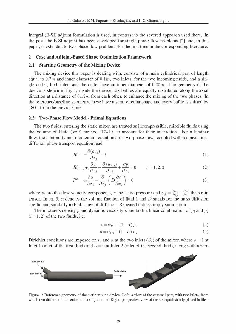
N. Galanos, E.M. Papoutsis-Kiachagias, and K.C. Giannakoglou
Integral (E-SI) adjoint formulation is used, in contrast to the severed approach used there. In
the past, the E-SI adjoint has been developed for single-phase flow problems [2] and, in this
paper, is extended to two-phase flow problems for the first time in the corresponding literature.
2 Case and Adjoint-Based Shape Optimization Framework
2.1 Starting Geometry of the Mixing Device
The mixing device this paper is dealing with, consists of a main cylindrical part of length
equal to 0.7m and inner diameter of 0.1m, two inlets, for the two incoming fluids, and a sin-
gle outlet; both inlets and the outlet have an inner diameter of 0.05m. The geometry of the
device is shown in fig. 1; inside the device, six baffles are equally distributed along the axial
direction at a distance of 0.12m from each other, to enhance the mixing of the two phases. In
the reference/baseline geometry, these have a semi-circular shape and every baffle is shifted by
180◦ from the previous one.
2.2 Two-Phase Flow Model - Primal Equations
The two fluids, entering the static mixer, are treated as incompressible, miscible fluids using
the Volume of Fluid (VoF) method [17–19] to account for their interaction. For a laminar
flow, the continuity and momentum equations for two-phase flows coupled with a convection-
diffusion phase transport equation read
Rp=−∂(ρvj)
∂xj
=0 (1)
Rvi =ρvj
∂vi∂xj
− ∂ (μεij)
∂xj
+∂p
∂xi
=0 , i = 1, 2, 3 (2)
Rα=vi∂α
∂xi
− ∂
∂xj
(D
∂α
∂xj
)=0 (3)
where vi are the flow velocity components, p the static pressure and εij =∂vi∂xj
+∂vj∂xi
the strain
tensor. In eq. 3, α denotes the volume fraction of fluid 1 and D stands for the mass diffusion
coefficient, similarly to Fick’s law of diffusion. Repeated indices imply summation.
The mixture’s density ρ and dynamic viscosity μ are both a linear combination of ρi and μi
(i=1, 2) of the two fluids, i.e.
ρ=αρ1+(1−α) ρ2 (4)
μ=αμ1+(1−α)μ2 (5)
Dirichlet conditions are imposed on vi and α at the two inlets (SI) of the mixer, where α=1 at
Inlet 1 (inlet of the first fluid) and α=0 at Inlet 2 (inlet of the second fluid), along with a zero
Figure 1: Reference geometry of the static mixing device. Left: a view of the external part, with two inlets, from
which two different fluids enter, and a single outlet. Right: perspective view of the six equidistantly placed baffles.
58

N. Galanos, E.M. Papoutsis-Kiachagias, and K.C. Giannakoglou
Neumann condition on p. At the single outlet (SO), zero Neumann conditions are imposed on
both vi and α along with a constant (zero) value for p. Finally, at the solid walls (SW ), a zero
Dirichlet (no-slip) condition is imposed on vi and zero Neumann conditions on p and α.
2.3 Shape Parameterization
A volumetric B-Splines morphing technique is employed to parameterize the shape of the
baffles. Let X ijkm ,m∈ [1, 3], i∈ [0, I], j∈ [0, J ], k∈ [0, K] be the value of the m−th coordinate
in the cylindrical system of the ijk− th control point in the 3D control grid. These values
constitute the design variables of the problem, i.e. the optimization unknowns. The cylindrical
coordinates x=[r, θ, z] of the grid points residing within the morphing lattice are given by
xm(u, v, w)=Ui,pu(u)Vj,pv(v)Wk,pw(w)Xijkm (6)
where u = [u, v, w] denotes the grid parametric coordinates. U, V,W are the B-Splines basis
functions and pu, pv, pw their corresponding polynomial degree, which may be different per
control point direction. A single control lattice parameterizing the shape of a single baffle, as
well as the grid points neighboring to the same baffle, is presented in fig. 2.
2.4 The Continuous Adjoint Method
In what follows, bn,n ∈ [1, N ] is used to denote the design variables. Two objective func-
tions to be minimized, are considered. The first one expresses the volume-averaged mixture
uniformity at the outlet of the device, written as
JU =1
2
∫SO
vini(α− α)2dS , α =1
|SO|
∫SO
αdS (7)
where ni are the components of the unit normal vector pointing outwards of the flow domain
and α is the mean value of the volume fraction computed at the outlet. The second objective
function is the volume-averaged total pressure losses between the inlet(s) and the outlet,
JP = −∫SI,O
vini
(p+
1
2ρv2j
)dS (8)
The derivatives of the two objective functions w.r.t. the design variables bn are computed and
used to minimize their weighted sum
J=w1JU+w2JP (9)
Figure 2: A control grid consisted of 7 points
in the radial direction, 7 points in the periph-
eral direction and 5 points in the mixer’s lon-
gitudinal direction, used to parameterize the
shape of a single baffle. Control points in blue
remain fixed during the optimization. Those
in red, are active and may change the baffle’s
shape.
59

N. Galanos, E.M. Papoutsis-Kiachagias, and K.C. Giannakoglou
∂jSi
∂pni
∂jSk
∂vink
∂jSi
∂αni
JU 01
2(α− α)2 nkδ
ki vini (α− α)
JP −vini −(p+
1
2ρv2j
)nkδ
ki −ρvknkvi −vini
1
2ρΔv
2j
Table 1: Derivatives of integrands jSiof the two objective functions w.r.t. the flow variables.
where w1,w2 are user-defined weights. By performing a number of single-objective runs with
different sets of weights, the front of non-dominated solutions in the objective space can be
computed. To facilitate the development of the adjoint, J is written in the form of two surface
integrals along SI and SO, as follows
J=
∫SI
jSI,inidS+
∫SO
jSO,inidS (10)
UsingδΦ
δbn=
∂Φ
∂bn+
∂Φ
∂xk
δxk
δbnto link the total derivative
δ
δbnof any flow quantity Φ w.r.t. bn, the
partial derivative∂
∂bnand grid sensitivities
δxk
δbn, the differentiation of eq. 10 w.r.t. bn gives
δJ
δbn=
∫SI,O
∂jSi
∂bnnidS+
∫SI,O
∂jSi
∂xk
δxk
δbnnidS+
∫SI,O
jSi
δ (nidS)
δbn(11)
where (see, also, table 1)
∂jSi
∂bnni=
∂jSk
∂vi
∂vi∂bn
nk+∂jSi
∂p
∂p
∂bnni+
∂jSi
∂α
∂α
∂bnni (12)
The development of the E-SI adjoint starts by defining the Lagrangian
L=J+
∫Ω
qRpdΩ+
∫Ω
uiRvi dΩ+
∫Ω
ψRαdΩ+
∫Ω
mαi R
mi dΩ (13)
where q is the adjoint pressure, ui are the components of the adjoint velocity and ψ is the adjoint
volume fraction. Apart from integrals including the equations pertaining to the two-phase flow,
L also includes grid displacement PDEs to account for variations in the nodal coordinates of
the computational grid due to the changes in the design variables. Herein, a Laplace type grid
displacement model, as firstly proposed in [2] for single-phase flows, is assumed
Rmi =
∂2mi
∂x2j
=0 , i = 1, 2, 3 (14)
where mi denote grid nodal displacements and mαi their adjoint. The fact that eqs. 14 are
included in L does not imply that this model should necessarily be used to displace the internal
grid nodes during the optimization. This is just a convenient, though harmless, assumption
(see [15]) made during the development of the E-SI adjoint.
Differentiating L w.r.t. bn gives
δL
δbn=
δJ
δbn+
∫Ω
q∂Rp
∂bndΩ+
∫Ω
ui∂Rv
i
∂bndΩ+
∫Ω
ψ∂Rα
∂bndΩ+
∫Ω
mαi
∂Rmi
∂bndΩ
+
∫S
(qRp+uiRvi +ψRα+mα
i Rmi )
δxk
δbnnkdS
(15)
60

N. Galanos, E.M. Papoutsis-Kiachagias, and K.C. Giannakoglou
where the last term emerges from the application of the Leibniz integral rule. The rest of the
integrals appearing on the r.h.s. of eq. 15 can further be developed using the Gauss divergence
theorem and∂
∂bn
(∂Φ
∂xj
)=
∂
∂xj
(∂Φ
∂bn
), according to which spatial and partial derivatives
w.r.t. bn permute. The mathematical development of the first three volume integrals can be
found in [1]. The last volume integral on the r.h.s. of eq. 15 becomes∫Ω
mαk
∂Rmk
∂bndΩ=
∫S
mαknj
∂
∂xj
(δxk
δbn
)dS−
∫S
∂mαk
∂xj
njδxk
δbndS+
∫Ω
∂2mαk
∂x2j
δxk
δbndΩ (16)
2.4.1 Adjoint Equations
To avoid the computation of partial derivatives of p, vi and α w.r.t. bn in the interior of the
flow domain, their multipliers inside field integrals in (the developed form of) eq. 15 are set to
zero, giving rise to the adjoint set of PDEs, which take the following form (being the same in
both the E-SI and FI adjoint formulations)
Rq=−∂ui
∂xi
=0 (17)
Rui =ρuj
∂vj∂xi
− ∂(ρvjui)
∂xj
−∂(μεαij
)∂xj
+ρ∂q
∂xi
+ψ∂α
∂xi
=0 , i = 1, 2, 3 (18)
Rψ=−∂ (vjψ)
∂xj
− ∂
∂xj
(D
∂ψ
∂xj
)+ρΔ
(vi
∂q
∂xi
+ uivj∂vi∂xj
)+μΔ
∂ui
∂xj
εij=0 (19)
where ρΔ=ρ1−ρ2, μΔ=μ1−μ2 and εαij=∂ui
∂xj+
∂uj
∂xiis the adjoint strain tensor.
The surface integrals arising from the use of the Leibniz integral rule are transformed to
volume integrals ofδxk
δbn, [2], according to
∫S
ΨRδxk
δbnnkdS =
∫Ω
Ψ∂R
∂xk
δxk
δbndΩ, where Ψ =
{q, ui, ψ} denotes every adjoint variable and R = {Rp, Rvi , R
α} the residual of the corre-
sponding primal problem. By expanding these terms and eliminating the multipliers ofδxk
δbn,
to avoid their computation in the interior of the domain, the adjoint grid displacement PDEs
arise, namely
Rmα
k =∂2mα
k
∂x2j
− ∂
∂xj
{q∂ (ρvj)
∂xk
−ρuivj∂vi∂xk
−uj∂p
∂xk
+ui∂ (μεij)
∂xk
−μεαij∂vi∂xk
−ψvj∂α
∂xk
−D∂ψ
∂xj
∂α
∂xk
+Dψ∂2α
∂xk∂xj
}=0 , k = 1, 2, 3
(20)
2.4.2 Adjoint Boundary Conditions
The field adjoint equations are associated with the following boundary conditions:
• Inlets (SI): Zero Dirichlet and zero Neumann conditions are imposed on ψ and q, respec-
tively. For the normal component of the adjoint velocity u〈n〉 =−∂jSI,i
∂pni, whereas the
tangential components are set to zero uI〈t〉=uII
〈t〉= 0.
61

N. Galanos, E.M. Papoutsis-Kiachagias, and K.C. Giannakoglou
• Outlet (SO): A Robin condition −ρΔqvini−μΔuiεijnj+ψvjnj+D∂ψ
∂xj
nj+∂jSO,j
∂αnSO,j
=0 is
imposed on ψ. Dirichlet conditions of the form q=u〈n〉v〈n〉+2ν∂u〈n〉∂n
+1
ρ
∂jSO,k
∂vinSO,k
ni and
v〈n〉u〈t〉+ν
(∂u〈t〉∂n
+∂u〈n〉∂t
)+1
ρ
∂jSO,k
∂vinSO,k
ti=0 are imposed on q and ui, respectively.
• Solid Walls (SW ): A zero Dirichlet boundary condition is imposed on ui along with zero
Neumann conditions on ψ and q.
On the adjoint grid displacement fields mαi , a zero Dirichlet condition mα
k =0 is imposed along
all the boundaries of the domain.
2.4.3 Sensitivity Derivatives
After satisfying the adjoint field equations and their boundary conditions, the remaining
terms in (the developed form of) eq. 15 stand for the E-SI adjoint SDs, namely
δJ
δbn
∣∣∣∣E−SI
= −∫SW
[(−ρqni + μεαijnj
) ∂vi∂xj
nk+∂mα
k
∂xj
−Dψ∂2α
∂xk∂xj
]δxk
δbnnjdS
+
∫SW
Dψ∂α
∂xj
δnj
δbndS
(21)
3 On the accuracy of the Sensitivity Derivatives using the Adjoint Formutations
Before proceeding to the application of the proposed method, two studies are carried out
to demonstrate (a) the accuracy of the computed derivatives using the adjoint method and (b)
the advantages of solving the adjoint to the grid displacement model PDEs accordingly to the
E-SI adjoint formulation. In both studies, the flow Reynolds number is � 350 and the flow
is assumed to be laminar. Also, the properties of the two fluids under consideration remain
the same (see table 2) with the diffusion coefficient D = 1.5 ·10−7m2/s. For the purpose of
comparison, SDs are computed using both the E-SI and severed E-SI adjoints; in the latter, also
abbreviated as SI adjoint, the contribution of the adjoint grid displacement field is omitted from
the SDs. Adjoint sensitivities are, also, compared to Finite Differences (FDs).
Firstly, SDs are computed for JP (eq. 8) in two different 2D geometries/cases. Regarding
case 1, a 2D duct with two inlets, from which two different fluids enter the domain, is con-
sidered; case 2 pertains to a 2D U-bend duct, the inlet of which is split in half for the two
incoming fluids. About 140K and 84K cells, respectively (see fig. 3) were used in each case;
both grids are adequately stretched close to the wall in order to resolve the flow boundary layers.
B-Splines morphing lattices parameterized the duct’s convergent part in case 1 and the duct’s
U turn in case 2. In fig. 3, the control boxes used in each case are demonstrated. The SDs of
JP w.r.t. the displacements of the active control points in the x and y direction, are computed
and plotted in fig. 4. SDs computed based on the E-SI adjoint formulation perfectly match FDs.
Exceptionally, in both cases, the SDs based on the SI adjoint (i.e. by omitting the solution of the
adjoint grid displacement PDEs) are quite accurate. However, this is a conclusion that cannot
be generalized.
Additionally, in case 2, SDs are computed for a different objective function, namely the mean
value of α at the exit
Jα=1
|SO|
∫SO
αdS (22)
62
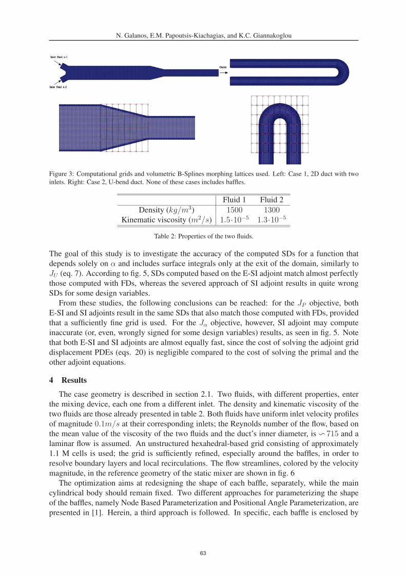
N. Galanos, E.M. Papoutsis-Kiachagias, and K.C. Giannakoglou
Figure 3: Computational grids and volumetric B-Splines morphing lattices used. Left: Case 1, 2D duct with two
inlets. Right: Case 2, U-bend duct. None of these cases includes baffles.
Fluid 1 Fluid 2
Density (kg/m3) 1500 1300Kinematic viscosity (m2/s) 1.5·10−5 1.3·10−5
Table 2: Properties of the two fluids.
The goal of this study is to investigate the accuracy of the computed SDs for a function that
depends solely on α and includes surface integrals only at the exit of the domain, similarly to
JU (eq. 7). According to fig. 5, SDs computed based on the E-SI adjoint match almost perfectly
those computed with FDs, whereas the severed approach of SI adjoint results in quite wrong
SDs for some design variables.
From these studies, the following conclusions can be reached: for the JP objective, both
E-SI and SI adjoints result in the same SDs that also match those computed with FDs, provided
that a sufficiently fine grid is used. For the Jα objective, however, SI adjoint may compute
inaccurate (or, even, wrongly signed for some design variables) results, as seen in fig. 5. Note
that both E-SI and SI adjoints are almost equally fast, since the cost of solving the adjoint grid
displacement PDEs (eqs. 20) is negligible compared to the cost of solving the primal and the
other adjoint equations.
4 Results
The case geometry is described in section 2.1. Two fluids, with different properties, enter
the mixing device, each one from a different inlet. The density and kinematic viscosity of the
two fluids are those already presented in table 2. Both fluids have uniform inlet velocity profiles
of magnitude 0.1m/s at their corresponding inlets; the Reynolds number of the flow, based on
the mean value of the viscosity of the two fluids and the duct’s inner diameter, is � 715 and a
laminar flow is assumed. An unstructured hexahedral-based grid consisting of approximately
1.1 M cells is used; the grid is sufficiently refined, especially around the baffles, in order to
resolve boundary layers and local recirculations. The flow streamlines, colored by the velocity
magnitude, in the reference geometry of the static mixer are shown in fig. 6
The optimization aims at redesigning the shape of each baffle, separately, while the main
cylindrical body should remain fixed. Two different approaches for parameterizing the shape
of the baffles, namely Node Based Parameterization and Positional Angle Parameterization, are
presented in [1]. Herein, a third approach is followed. In specific, each baffle is enclosed by
63
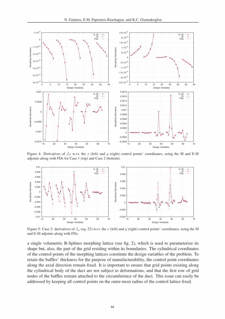
N. Galanos, E.M. Papoutsis-Kiachagias, and K.C. Giannakoglou
−6×10⁻⁶
−5×10⁻⁶
−4×10⁻⁶
−3×10⁻⁶
−2×10⁻⁶
−1×10⁻⁶
0
1×10⁻⁶
0 5 10 15 20 25 30 35 40
Sen
sitiv
ity D
eriv
ativ
e
Design Variables
E−SISI
FDs
−2.5×10⁻⁵
−2×10⁻⁵
−1.5×10⁻⁵
−1×10⁻⁵
−5×10⁻⁶
0
5×10⁻⁶
1×10⁻⁵
1.5×10⁻⁵
2×10⁻⁵
2.5×10⁻⁵
0 5 10 15 20 25 30 35 40
Sen
sitiv
ity D
eriv
ativ
e
Design Variables
E−SISI
FDs
−0.0015
−0.001
−0.0005
0
0.0005
0.001
10 20 30 40 50 60 70
Sen
sitiv
ity D
eriv
ativ
e
Design Variables
E−SISI
FDs
−0.0004
−0.0002
0
0.0002
0.0004
0.0006
0.0008
0.001
0.0012
0.0014
0.0016
0.0018
10 20 30 40 50 60 70
Sen
sitiv
ity D
eriv
ativ
e
Design Variables
E−SISI
FDs
Figure 4: Derivatives of JP w.r.t. the x (left) and y (right) control points’ coordinates, using the SI and E-SI
adjoints along with FDs for Case 1 (top) and Case 2 (bottom).
−0.01
−0.008
−0.006
−0.004
−0.002
0
0.002
0.004
0.006
0.008
0.01
10 20 30 40 50 60 70
Sen
sitiv
ity D
eriv
ativ
e
Design Variables
E−SISI
FDs
−0.004
−0.002
0
0.002
0.004
0.006
0.008
0.01
10 20 30 40 50 60 70
Sen
sitiv
ity D
eriv
ativ
e
Design Variables
E−SISI
FDs
Figure 5: Case 2: derivatives of Jα (eq. 22) w.r.t. the x (left) and y (right) control points’ coordinates, using the SI
and E-SI adjoints along with FDs.
a single volumetric B-Splines morphing lattice (see fig. 2), which is used to parameterize its
shape but, also, the part of the grid residing within its boundaries. The cylindrical coordinates
of the control points of the morphing lattices constitute the design variables of the problem. To
retain the baffles’ thickness for the purpose of manufacturability, the control point coordinates
along the axial direction remain fixed. It is important to ensure that grid points existing along
the cylindrical body of the duct are not subject to deformations, and that the first row of grid
nodes of the baffles remain attached to the circumference of the duct. This issue can easily be
addressed by keeping all control points on the outer-most radius of the control lattice fixed.
64

N. Galanos, E.M. Papoutsis-Kiachagias, and K.C. Giannakoglou
Figure 6: Stream-lines colored by the velocity magnitude in the reference geometry.
w1 1 0.5 0.25 0.2 0.1 0
w2 0 0.5 0.75 0.8 0.9 1
Table 3: Weight combinations used in the objective function J (eq. 10).
The E-SI adjoint formulation (eq. 21) is used to compute the derivatives of the weighted
objective function (eq. 10) w.r.t. the coordinates of the control points. For six weight combi-
nations, see table 3, the Pareto front of non-dominated solutions in the two-objective space is
computed and plotted in fig. 7; there, the values of JU and JP have been divided by the known
volume flow rate.
As shown in fig. 7, minimization of total pressure losses and maximization of the mixture’s
uniformity at the exit are two contradictory targets. For instance, in case with w1 = 1, w2 = 0,
the optimization leads to a huge increase in uniformity (decrease in JU ) by 94% at the exit,
0
0.0002
0.0004
0.0006
0.0008
0.001
0.0012
0.0014
0.0016
0.0018
65 70 75 80 85 90 95 100 105 110 115 120
Mix
ture
Uni
form
ity [−
]
Total Pressure Losses [Pa]
(w1, w2)
(1.00, 0.00)(0.50, 0.50)
(0.25, 0.75)(0.20, 0.80)
(0.10, 0.90)
(0.00, 1.00) reference geometry
Figure 7: The front of non-dominated optimal solutions in the two objective space computed by the six weight
combinations of table 3.
65
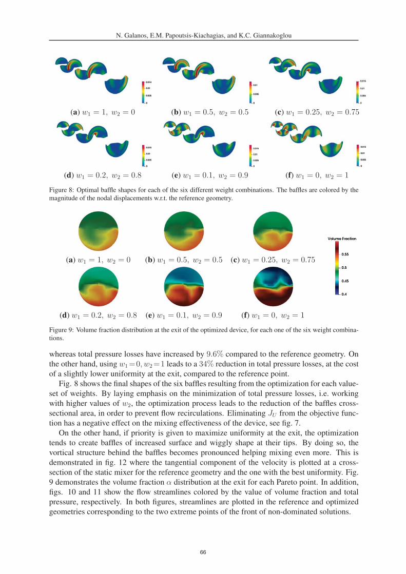
N. Galanos, E.M. Papoutsis-Kiachagias, and K.C. Giannakoglou
(a) w1 = 1, w2 = 0 (b) w1 = 0.5, w2 = 0.5 (c) w1 = 0.25, w2 = 0.75
(d) w1 = 0.2, w2 = 0.8 (e) w1 = 0.1, w2 = 0.9 (f) w1 = 0, w2 = 1
Figure 8: Optimal baffle shapes for each of the six different weight combinations. The baffles are colored by the
magnitude of the nodal displacements w.r.t. the reference geometry.
(a) w1 = 1, w2 = 0 (b) w1 = 0.5, w2 = 0.5 (c) w1 = 0.25, w2 = 0.75
(d) w1 = 0.2, w2 = 0.8 (e) w1 = 0.1, w2 = 0.9 (f) w1 = 0, w2 = 1
Figure 9: Volume fraction distribution at the exit of the optimized device, for each one of the six weight combina-
tions.
whereas total pressure losses have increased by 9.6% compared to the reference geometry. On
the other hand, using w1=0, w2=1 leads to a 34% reduction in total pressure losses, at the cost
of a slightly lower uniformity at the exit, compared to the reference point.
Fig. 8 shows the final shapes of the six baffles resulting from the optimization for each value-
set of weights. By laying emphasis on the minimization of total pressure losses, i.e. working
with higher values of w2, the optimization process leads to the reduction of the baffles cross-
sectional area, in order to prevent flow recirculations. Eliminating JU from the objective func-
tion has a negative effect on the mixing effectiveness of the device, see fig. 7.
On the other hand, if priority is given to maximize uniformity at the exit, the optimization
tends to create baffles of increased surface and wiggly shape at their tips. By doing so, the
vortical structure behind the baffles becomes pronounced helping mixing even more. This is
demonstrated in fig. 12 where the tangential component of the velocity is plotted at a cross-
section of the static mixer for the reference geometry and the one with the best uniformity. Fig.
9 demonstrates the volume fraction α distribution at the exit for each Pareto point. In addition,
figs. 10 and 11 show the flow streamlines colored by the value of volume fraction and total
pressure, respectively. In both figures, streamlines are plotted in the reference and optimized
geometries corresponding to the two extreme points of the front of non-dominated solutions.
66

N. Galanos, E.M. Papoutsis-Kiachagias, and K.C. Giannakoglou
Figure 10: Stream-lines colored by the value of the volume fraction α for the reference (left), and the optimized
geometry for min. JU (right).
Figure 11: Stream-lines colored by the value of the total pressure for the reference (left), and the optimized
geometry for min. JP (right).
Figure 12: Velocity vectors lying on a cross-section at the middle of the static mixer’s length in the reference (left)
and optimized for mixture uniformity (right) geometries. In the latter, a highly vortical flow that enhances mixing
appears.
5 Conclusions
In this paper, the continuous adjoint method to a two-phase flow model for laminar flows
was utilized for the optimization of a mixing device with baffles. Previous works [1], also
conducted by the authors’ group, where the “severed” adjoint approach was followed, were
herein extended, in order to account for the effect of grid sensitivities during the computation
67

N. Galanos, E.M. Papoutsis-Kiachagias, and K.C. Giannakoglou
of SDs. The Enhanced-SI (E-SI) adjoint formulation was presented and, then, was used for the
optimization of the baffles’ shapes by considering two objectives, namely minimization of total
pressure losses and maximization of the mixture’s uniformity at the exit. First, two studies were
conducted in order to assess the accuracy of the computed SDs using the two adjoints, with a
reasonable computational cost. There, it was shown that the E-SI and SI adjoints may differ
depending on the objective function, with the former computing SDs in good agreement with
FDs and the latter occasionally deviating from them.
Regarding the static mixer problem, six optimization runs were performed in total, each of
which resulted to optimal baffles of different shapes; the parameterization scheme used, namely
a volumetric B-Splines morphing technique, ensured that the baffles’ thickness remained fixed
during the optimization and their peripheral part remained attached to the body of the mixer.
So, the Pareto front of non-dominated solutions in the two-objective space was generated. Each
optimal baffle configuration pertains to a single Pareto point; the two extreme points, in spe-
cific, indicate two different mechanisms for improving mixing performance and decreasing total
pressure losses which are, in fact, contradictory goals. To conclude, a highly uniform mixture
at the exit requires wiggly baffles that tend to increase the flow vorticity, whereas decreasing
total pressure drop is achieved by creating smaller baffles to minimally disturb the flow.
REFERENCES
[1] P. Alexias, K.C. Giannakoglou, Optimization of a static mixing device with baffles using
the continuous adjoint to a two-phase mixing model. Optimization and Engineering, 21,
631–650, 2020.
[2] I.S. Kavvadias, E.M. Papoutsis-Kiachagias, K.C. Giannakoglou, On the proper treatment
of grid sensitivities in continuous adjoint methods for shape optimization. Journal ofComp. Physics, 301, 1-18, 2015.
[3] E.M. Papoutsis-Kiachagias, K.C. Giannakoglou, Continuous adjoint methods for turbulent
flows, applied to shape and topology optimization: industrial applications. Archives ofComputational Methods in Engineering, 23, 255–299, 2016.
[4] K.T. Gkaragkounis, E.M. Papoutsis-Kiachagias, K.C. Giannakoglou, The continuous ad-
joint method for shape optimization in Conjugate Heat Transfer problems with turbulent
incompressible flows. Applied Thermal Engineering, 140, 351–362, 2018.
[5] E.M. Papoutsis-Kiachagias, K.T. Gkaragkounis, A.I. Margetis, T. Skamagkis, V.G. Asouti,
K.C. Giannakoglou, adjointOptimisationFoam: An OpenFOAM-based framework for
adjoint-assisted optimization. In 14–th ECCOMAS Thematic Conference on Evolution-ary and Deterministic Methods for Design, Optimization and Control (EUROGEN 2021),Athens, Greece, 17–19 May, 2021.
[6] E.B. Nauman, Enhancement of heat transfer and thermal homogeneity with motionless
mixers. AIChE Journal, 25, 246-258, 1979.
[7] H.P. Grace, Dispersion phenomena in high viscosity immiscible fluid systems and appli-
cation of static mixers as dispersion in such systems. Chem. Eng. Communications, 24,
225–277, 1982.
68

N. Galanos, E.M. Papoutsis-Kiachagias, and K.C. Giannakoglou
[8] S.S. Soman, C.M.R. Madhuranthakam, Effects of internal geometry modifications on the
dispersive and distrubutive mixing in static mixers. Chem. Eng. and Processing, 122, 31–
43, 2017.
[9] H. Song, S.P. Han, A general correlation for pressure drop in kenics static mixer. Chem.Eng. Science, 60, 5696–5704, 2005.
[10] B. Kwon, L. Liebenberg, A.M. Jacobi, W.P. King, Heat transfer enhancement of internal
laminar flows using additively manufactured static mixers. Int. Journal of Heat and MassTransfer, 137, 292–300, 2019.
[11] A. Jameson, Aerodynamic design via control theory. Journal of Scientific Computing, 3,
233–260, 1988.
[12] W.K. Anderson, V. Venkatakrishnan, Aerodynamic design optimization on unstructured
grids with a continuous adjoint formulation. Computers & Fluids, 28, 443–480, 1999.
[13] A. Jameson, S. Kim, Reduction of the adjoint gradient formula in the continuous limit. In
41th Aerospace Sci. Meeting and Exhibit, Reno, Nevada, 2003, AIAA 2003–0040.
[14] D.I. Papadimitriou, K.C. Giannakoglou, A continuous adjoint method with objective func-
tion derivatives based on boundary integrals for inviscid and viscous flows. Computers &Fluids, 36, 325–341, 2007.
[15] K.T. Gkaragkounis, E.M. Papoutsis-Kiachagias, A.G. Tsolovikos, K.C. Giannakoglou, Ef-
fect of Grid Displacement Models on Sensitivity Derivatives computed by the Continuous
Adjoint in Aerodynamic and Conjugate Heat Transfer Shape Optimization. EngineeringOptimization, 2020 (to appear).
[16] C. Brennen, Fundamentals of multiphase flow. Cambridge University Press, Cambridge,
2005.
[17] M. Ishii, T. Hibiki, Thermo-fluid dynamics of two-phase flow. Springer, New York, USA,
2011.
[18] M.M. Francois, S.J. Cummins, E.D. Dendy, D.B. Kothe, J.M. Sicilian, M.W. Williams,
A balanced-force algorithm for continuous and sharp interfacial surface tension models
within a volume tracking framework. Journal of Comp. Physics, 213, 141–173, 2006.
[19] S. Popinet, An accurate adaptive solver for surface-tension driven interracial flows. Jour-nal of Comp. Physics, 228, 5838–5866, 2009.
69

CONTINUOUS ADJOINT–BASED AEROACOUSTIC SHAPEOPTIMIZATION OF AN AERO–ENGINE INTAKE
M. Monfaredi1, V.G. Asouti1, X.S. Trompoukis1, K.T. Tsiakas1 and K.C. Giannakoglou1
1National Technical University of Athens,Parallel CFD & Optimization Unit, School of Mechanical Engineering
Zografou Campus, 9 Iroon Polytechniou Stre-mail:[email protected], [email protected], [email protected],
[email protected] and [email protected]
Keywords: Aeroacoustic, Continuous adjoint, Shape optimization, FW-H analogy, Aero–engine
Intake
Abstract. This paper addresses the aeroacoustic shape optimization of a 3D aero-engineintake by means of gradient-based optimization assisted by continuous adjoint. A hybrid aeroa-coustic model based on the (U)RANS equations and the permeable version of the FfowcsWilliams-Hawkings (FW-H) acoustic analogy in the frequency domain is used. The flow andadjoint simulations are for compressible fluid flows realized using the in–house GPU–enabledsoftware PUMA. The continuous adjoint formulation includes the differentiation of the Spalart–Allmaras turbulence model. The implementation and differentiation of the 3D FW–H analogyare verified by comparing the results of the FW–H analogy to both analytical solutions andURANS. In order to save computational cost, periodic boundary conditions are used to reducethe solution domain size together with the use of a moving reference frame which leads to steadyflow and adjoint runs. The generatrix of the nacelle lips and the throat area are parameterizedusing NURBS. The developed tool is used to perform shape optimization to minimize the totalenergy contained in the spectrum of the sound pressure, at prescribed receiver locations.
EUROGEN 2021 14th ECCOMAS Thematic Conference on
Evolutionary and Deterministic Methods for Design, Optimization and Control N. Gauger, K. Giannakoglou, M. Papadrakakis, J. Periaux (eds.)
Streamed from Athens, Greece, – 2021
70
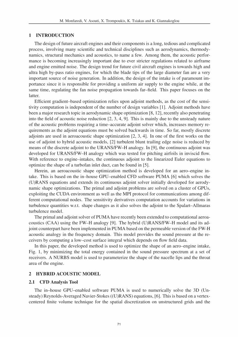
M. Monfaredi, V. Asouti, X. Trompoukis, K. Tsiakas and K. Giannakoglou
1 INTRODUCTION
The design of future aircraft engines and their components is a long, tedious and complicated
process, involving many scientific and technical disciplines such as aerodynamics, thermody-
namics, structural mechanics and acoustics, to name a few. Among them, the acoustic perfor-
mance is becoming increasingly important due to ever stricter regulations related to airframe
and engine emitted noise. The design trend for future civil aircraft engines is towards high and
ultra high by-pass ratio engines, for which the blade tips of the large diameter fan are a very
important source of noise generation. In addition, the design of the intake is of paramount im-
portance since it is responsible for providing a uniform air supply to the engine while, at the
same time, regulating the fan noise propagation towards far–field. This paper focuses on the
latter.
Efficient gradient–based optimization relies upon adjoint methods, as the cost of the sensi-
tivity computation is independent of the number of design variables [1]. Adjoint methods have
been a major research topic in aerodynamic shape optimization [8, 12], recently also penetrating
into the field of acoustic noise reduction [2, 3, 4, 9]. This is mainly due to the unsteady nature
of the acoustic problems requiring a time–accurate adjoint solver which, increases memory re-
quirements as the adjoint equations must be solved backwards in time. So far, mostly discrete
adjoints are used in aeroacoustic shape optimization [2, 3, 4]. In one of the first works on the
use of adjoint to hybrid acoustic models, [2] turbulent blunt trailing edge noise is reduced by
means of the discrete adjoint to the URANS/FW–H analogy. In [9], the continuous adjoint was
developed for URANS/FW–H analogy which was tested for pitching airfoils in inviscid flow.
With reference to engine–intakes, the continuous adjoint to the linearized Euler equations to
optimize the shape of a turbofan inlet duct, can be found in [5].
Herein, an aeroacoustic shape optimization method is developed for an aero–engine in-
take. This is based on the in–house GPU–enabled CFD software PUMA [6] which solves the
(U)RANS equations and extends its continuous adjoint solver initially developed for aerody-
namic shape optimizations. The primal and adjoint problems are solved on a cluster of GPUs,
exploiting the CUDA environment as well as the MPI protocol for communications among dif-
ferent computational nodes. The sensitivity derivatives computation accounts for variations in
turbulence quantities w.r.t. shape changes as it also solves the adjoint to the Spalart–Allmaras
turbulence model.
The primal and adjoint solver of PUMA have recently been extended to computational aeroa-
coustics (CAA) using the FW–H analogy [9]. The hybrid (U)RANS/FW–H model and its ad-
joint counterpart have been implemented in PUMA based on the permeable version of the FW-H
acoustic analogy in the frequency domain. This model provides the sound pressure at the re-
ceivers by computing a low–cost surface integral which depends on flow field data.
In this paper, the developed method is used to optimize the shape of an aero–engine intake,
Fig. 1, by minimizing the total energy contained in the sound pressure spectrum at a set of
receivers. A NURBS model is used to parameterize the shape of the nacelle lips and the throat
area of the engine.
2 HYBRID ACOUSTIC MODEL
2.1 CFD Analysis Tool
The in–house GPU–enabled software PUMA is used to numerically solve the 3D (Un-
steady) Reynolds-Averaged Navier-Stokes ((U)RANS) equations, [6]. This is based on a vertex-
centered finite volume technique for the spatial discretization on unstructured grids and the
71

M. Monfaredi, V. Asouti, X. Trompoukis, K. Tsiakas and K. Giannakoglou
Figure 1: Perspective view of the engine intake with a snapshot of isobar contours at the engine
inlet, serving as instantaneous boundary condition.
upwind second–order Roe approximation for the convection terms. The Spalart–Allmaras tur-
bulence model [7] is used. The software implements mixed–precision arithmetics according
to which the Jacobian of the residuals is computed in double– but stored in single–precision
which speeds up the computations and reduces the required GPU memory, without damaging
accuracy.
2.2 Noise Propagation Using The FW–H Analogy
Acoustic analogies propagate the flow–generated sound by means of analytical solutions
of the wave equation and this leads to a considerable reduction in computational cost [10].
The mathematical formulation of the permeable version of the FW-–H analogy, used herein,
originates from [11] for cases with a uniform mean flow (as in a wind tunnel), and reads(∂2
∂t2+u∞iu∞j
∂2
∂xi∂xj
+ 2u∞i
∂2
∂xi∂t−c2∞
∂2
∂xi∂xi
)(H(f)ρ′)=
∂
∂t(Qδ(f))− ∂
∂xi
(Fiδ(f)) (1)
where H(f) and δ(f) are the Heaviside and Dirac delta functions, respectively. Values f=0indicate the user–defined FW–H surface which should include all acoustic sources. Practically,
f is the signed distance from this surface, with negative and positive values corresponding to its
interior and exterior, respectively. The FW–H surface is located in the part of the grid which is
not displaced during the optimization. c∞ and �u∞ are the sound speed and velocity at far–field.
The quadrupole effects have not been included due to their small effect and the disproportionate
high computational cost. Only monopole (Q) and dipole (Fi) source terms
Q(�x, t) = (ρui − ρ∞u∞i)nFWH
i
Fi(�x, t) =[ρ (ui − 2u∞i) uj + ρ∞u∞iu∞j + pδij − τij
]nFWH
j
(2)
are retained. ρ = ρ∞+ ρ′, p = p∞+ p′ and ui = u∞i+u′i are the density, pressure and velocity
components, respectively, and the subscript ∞ indicates far–field quantities. �nFWH is the outward
unit vector normal to the FW–H surface.
72

M. Monfaredi, V. Asouti, X. Trompoukis, K. Tsiakas and K. Giannakoglou
The integral solution to eq. 1 provides the acoustic pressure at a receiver located at �xr. For
each frequency (ω) value, this yields
H(f)p′(�xr, ω) =−∫
f=0
Fi(�xs, ω)∂G(�xr, �xs, ω)
∂xsi
ds−∫
f=0
iωQ(�xs, ω)G(�xr, �xs, ω)ds (3)
where the hat ˆ symbol indicates quantities after transformation into the frequency domain using
Fourier transform, i is the unit complex number and �xs denotes position vectors of sources
located on the FW–H surface. In subsonic flows, the Green function for 3D problems in the
frequency domain is
G(�xr, �xs, ω) = −exp(−ikr+)
4πr∗(4)
where k = ω/c∞ is the wave number and
r+ =1
β2
(r∗ − �u∞ · �r
c∞
), r∗ =
√(�u∞ · �rc∞
)2
+ |�r|2 β2, �r = �xr − �xs (5)
Also, β =√1−M2 where M is the Mach number.
3 CONTINUOUS ADJOINT TO THE HYBRID ACOUSTIC MODEL
The aeroacoustic objective function J is defined in the frequency domain as the energy con-
tained in the sound spectrum
J =1
Nr
Nr∑a=1
∫ω
|p′(�xra , ω)|dω (6)
where p′(�xra , ω) is the outcome of eq. 3 and Nr is the number of receivers. |p′| =√p′2Re + p
′2Im,
where subscripts Re and Im denote the real and imaginary parts of complex variables. For the
purpose of this study, integration in eq. 6 degenerates to a single frequency value, namely that
of the main (tonal) frequency.
To formulate the adjoint problem, an augmented objective function is defined as Jaug = J +∫Ts
∫Ω
ΨnRndΩdt, where Ψn, Rn and Ω are the adjoint variable fields, the residuals of the unsteady
flow including Spalart–Allmaras turbulence model equations and the CFD domain, respectively.
Ts is the time window of the unsteady solution. By differentiating Jaug w.r.t. design variable
be (e=1, N with N being the number of design variables) and setting the multipliers of the
derivatives of the flow variables w.r.t. be equal to zero within the field and along the boundaries,
the unsteady adjoint equations and their boundary conditions are obtained as (only for the mean–
flow equation; for the adjoint to the Spalart–Allmaras model, the reader should refer to [13])
−∂Ψm
∂t− ∂f inv
nk
∂Um
∂Ψn
∂xk
−(∂τadjqk
∂xk
− ∂Ψ5
∂xk
τkq
) ∂uq
∂Um
− ∂qadjk
∂xk
∂T
∂Um
− ∂J
∂Um
δ(f) = 0 (7)
where Um, T and f invnk are the conservative flow variables, temperature and inviscid fluxes,
respectively, and
τadjmk = (μ+ μt)
[∂Ψm+1
∂xk
+∂Ψk+1
∂xm
+∂Ψ5
∂xm
uk +∂Ψ5
∂xk
um − 2
3δmk
(∂Ψl+1
∂xl
+∂Ψ5
∂xl
ul
)]qadjk = Cp
(μ
Pr+
μt
Prt
)∂Ψ5
∂xk
73

M. Monfaredi, V. Asouti, X. Trompoukis, K. Tsiakas and K. Giannakoglou
The last term in eq. 7 is defined only along the permeable FW–H surface. For the differentiation
of this term one should refer to [9]. The adjoint boundary condition along the solid walls is
Ψm+1nm = 0, where �n is the unit normal to the wall. Also, qadjk nk = 0 is imposed along the
adiabatic walls. The sensitivities of J w.r.t. design variables can be computed as
δJ
δbe=−
∫Ts
∫Ω
[Ψn
(∂f invnk
∂xi
− ∂f visnk
∂xi
)+ τadjmk
∂um
∂xi
+ qadjk
∂T
∂xi
] ∂
∂xk
(δxi
δbe
)dΩdt
+
∫Ts
∫S
(pΨk+1 −Ψnfinvnk +Ψ5qk +Ψ5umτmk)
δnk
δbedSdt
(8)
where f visnk and τmk are the viscous fluxes and stresses.
3.1 Verification of the FW-H Analogy Implementation
In the past, the implementation of the FW-H analogy in PUMA has been verified for 2D
cases [9]. In this section, the implementation is verified in a 3D problem. To do so, results of
the FW-H integral, eq. 3, are compared with the analytical solution of the sound field generated
by a monopole source in a uniform flow. Additionally, in order to verify the part of the code
that differentiates the FW–H integral, derivatives of the objective function, eq. 6, w.r.t. the
coordinates of the monopole source, �xs, are computed by the code and compared with the
outcome of a central second–order finite difference (FD) based on the analytical solution. The
monopole source is located at the origin of the coordinate system and is exposed to a uniform
flow u∞ along the +x direction, shown in 2a. The complex velocity potential of the case is
φ(�xr, �xs, ω) = A exp(iωt)exp(−ikr+)
4πr∗(9)
where r+ and r∗ are the same as in eq. 5 . The perturbation fields of flow variables are obtained
from the real parts of p′=−ρ∞(∂φ∂t+u∞1
∂φ∂x), u′ = ∇φ and ρ′=p′/c∞2. In this case, M∞ = 0.5,
A = 0.004 m2/s and ω = 3.095 rad/s. The FW-H surface is a cube extending from −0.5mto 0.5m in all three directions (see Fig. 2a), and is discretized by regular surface grids on the
six faces with 400 nodes on each face. The time history of p′ at a receiver located at �xr =(10m, 0m, 10m) as computed using the FW–H analogy shown in Fig. 2b perfectly matches the
analytical solution. Slight, practically not visible, differences in the plotted values are due to the
numerical integration on the FW-H surface. The derivatives w.r.t. to the source coordinates are
also compared in Fig. 2c. The agreement between finite differences of the analytical solution
and the differentiation of the FW-H is very good. As expected, the derivative w.r.t. xs2 is zero.
3.2 Optimization Framework For the Rotating Frame
Adjoint–based optimization in unsteady flows may become very demanding in terms of time
and memory. This is the main reason why the use of adjoint methods is comparatively restricted
in aeroacoustic shape optimization. In this particular application, in order to reduce the cost
and since the intake geometry is axisymmetric, a CFD domain that corresponds to a single
blade passage of the fan is used, with appropriate periodicity conditions. The flow and adjoint
equations are solved in a rotating (with the rotational speed of the engine) frame, thus leading
to a steady-state solution for both the flow and adjoint problems. A continuous circumferential
distribution of receivers at given radius and axial position is used for the computation of the
objective function of eq. 6. The workflow of the aeroacoustic optimization is shown in Fig. 3.
74

M. Monfaredi, V. Asouti, X. Trompoukis, K. Tsiakas and K. Giannakoglou
(a)
-0.0003
-0.0002
-0.0001
0
0.0001
0.0002
0.0003
0 5 10 15 20 25 30 35 40
P’ (
pa)
Time step
AnalyticalFW-H Integral
(b)
0
0.0005
0.001
0.0015
0.002
0.0025
0.003
1 2 3
δJ/
δx s
i
Monopole coordinate
FD of analytical solutionDifferentiated FW-H integral
(c)
Figure 2: Results of monopole sound source in flow for a receiver located at (10m, 0m, 10m). (a)
Schematic illustration of the monopole source, the FW-H surface and the receiver. (b) Compari-
son of the time history of pressure fluctuation within a period. (c) Comparison of the derivatives
of the acoustic objective function w.r.t. to the three coordinates (xsi , i=1, 2, 3) of the monopole
computed by the differentiation of the FW-H and FDs applied to the closed–form expressions.
4 SHAPE OPTIMIZATION OF THE AERO–ENGINE INTAKE
The above–described aeroacoustic analysis and optimization framework is applied to opti-
mize an air–engine intake. The aeroacoustic objective function to be minimized, i.e. that of
eq. 6, includes only the tonal noise. The geometry of a single blade passage shown in Fig. 4a
has about 3.7M nodes arranged on 100 meridional planes. The far–field flow is still and the
pressure distribution on the fan–inlet is used as boundary condition. The pressure contours on
the nacelle and mid–plane of the engine intake are plotted in Fig. 4b.
An axisymmetric parameterization model is adopted for the intake. The generatrix is firstly
reconstructed using NURBS and this gave rise to 15 design parameters controlling the shape of
the nacelle lips and the throat area, leaving its outer shape and the part close to the fan intact.
NURBS control points (CPs) are allowed to vary in both the axial and radial direction. Since
the first and last points are fixed, the optimization has 2×13=26 design variables, Fig. 5.
The FW–H surface, illustrated in Fig. 6a, has 16000 nodes. To perform the integration of
eq. 3, the FW–H surface should rotate to cover the full circumference. However, as a cheaper
75

M. Monfaredi, V. Asouti, X. Trompoukis, K. Tsiakas and K. Giannakoglou
Steady-state
flow solution
Rotate the flow field
and compute time
series of Q & Fi
on the FW-H surface
Fourier transform of Qand Fi. Compute the
FW-H integral, eq. 3
Compute
the objective
function, eq. 6
Adjoint to the
FW-H analogy
(compute ∂J∂Um
on
the FW-H surface)
Steady-state
adjoint
solution
Rotate the flow and
adjoint field. Compute
sensitivities, eq. 8
Initial geometry
Update the design
variables using a
descent method
Update the
geometry and grid
Figure 3: Workflow of the aeroacoustic optimization. Primal and adjoint parts are colored in
blue and orange, respectively.
(a) (b)
Figure 4: (a) Entire and close–up views of the CFD domain and the surface grid on one of
periodic boundaries. The parameterized part of the nacelle is colored in red. (b) Isobar contours
on the nacelle, mid–plane and engine inlet.
Nacelle generatrix
Active CPs
(1)(2)(3)(4)(5)(6)(7)(8)
(9)
(10)
(11)
(12)(13)
Figure 5: Distribution of the control points for the parameterization of the nacelle generatrix
using NURBS. The first and last control points are fixed during the optimization.
alternative, the receivers (instead of the FW–H surface) are rotated and the acoustic pressure is
retrieved by superimposing pressure signals from each receiver. As both the grid and numerical
set–up may affect the acoustic results, the outcome of the FW–H analogy is verified in the
current case as well. To do so, the acoustic pressure computed based on the hybrid model is
76

M. Monfaredi, V. Asouti, X. Trompoukis, K. Tsiakas and K. Giannakoglou
compared with that of the unsteady CFD code at 3 receiver locations, shown in Fig. 6a. The
CFD results match reasonably well those obtained by the FW–H analogy, Fig. 6b, given that
part of the discrepancies may be due to the neglect of quadrupole terms, representing the noise
due to viscous effects and turbulence.
(a)
-0.015
0
0.015
0 20 40 60 80 100
p’ (
pa)
Rec1CFD+FW-H
CFD
-0.08
-0.04
0
0.04
0.08
0 20 40 60 80 100
p’ (
pa)
Rec2
-0.015
0
0.015
0 20 40 60 80 100
p’ (
pa)
Time step
Rec3
(b)
Figure 6: (a) Location of the FW–H surface, in green, and 3 receivers within the CFD domain.
Streamlines are colored based on the pressure values. (b) Comparison of the pressure fluctua-
tions computed by CFD+FW–H with those obtained by pure CFD, at 3 different receivers.
The convergence history of the aeroacoustic objective function is presented in Fig. 7a. A
clear reduction in the objective value after 13 optimization cycles can be seen. This reduction
is also obvious in Fig. 7b that compares the amplitude of the sound pressure at a single receiver
in the baseline and the optimized geometries. Changes of the parameterized part of the nacelle
are illustrated in Fig. 8. As seen, the biggest geometrical change occurs at the nacelle lip
which is pushed forward, while minor changes occur elsewhere. Regarding the aerodynamic
performance, the optimized shape increases the total pressure loss by 0.6% compared to the
initial one. This could be expected as an acoustic objective was only considered.
0.2
0.3
0.4
0.5
0.6
0.7
0.8
0.9
1
2 4 6 8 10 12 14
Nor
mal
ized
noi
se
Optimization cycle
Noise objective
(a)
-0.08
-0.06
-0.04
-0.02
0
0.02
0.04
0.06
0.08
0 20 40 60 80 100
P’ (
pa)
Time step
Baseline
Optimized
(b)
Figure 7: (a) Convergence of the aeroacoustic objective value, normalized by its first cycle
value. (b) Comparison of the time history of the pressure fluctuation within a period at one
receiver.
77

M. Monfaredi, V. Asouti, X. Trompoukis, K. Tsiakas and K. Giannakoglou
(a) (b)
Figure 8: (a) Generatrix and (b) 3D view of the baseline and optimized geometry of the param-
eterized part of the nacelle.
5 CONCLUSIONS
This paper presented recent extensions of the analysis and adjoint–based optimization tool
of the in–house CFD solver PUMA in aeroacoustic shape optimization. A previous implemen-
tation of the permeable version of the FW–H analogy in the frequency domain, for 2D prob-
lems, is extended and verified in 3D, by comparing the results with the analytical solution of a
monopole source, including its differentiation. Based on this, a feasible 3D aeroacoustic noise
prediction and continuous adjoint–based shape optimization framework is developed for aero–
engine intake application which makes use of a steady flow and adjoint solution and builds the
unsteady field by rotating steady fields, overcoming the downsides of unsteady adjoint, namely
large memory requirement and long solution time.
The developed tool is used to optimize the shape of the nacelle lips and the throat area of
an aero–engine intake. The value of the aeroacoustic objective function is noticeably reduced
highlighting the functionality of the developed tool. Extensions to consider both aeroacoustic
and aerodynamic objectives in a multi-disciplinary framework are straightforward.
6 ACKNOWLEDGEMENTS
This work is part of the MADELEINE project which has received funding from the European
Union’s Horizon 2020 research and innovation programme under grant agreement No 769025.
The authors would like to thank Rolls-Royce plc. (Dr. S. Shahpar) and the research group of
the Institute of Sound and Vibration Research of the University of Southampton (Dr. L. Wu) for
providing the initial intake geometry and the boundary conditions of the fan inlet used herein.
REFERENCES
[1] A. Jameson, Aerodynamic design via control theory. Journal of Scientific Computing, 3,
233–260, 1988.
[2] M. Rumpfkeil, D.Zingg, A hybrid algorithm for far-field noise minimization. Computers& Fluids, 39, 1516–1528, 2010.
78

M. Monfaredi, V. Asouti, X. Trompoukis, K. Tsiakas and K. Giannakoglou
[3] B.Y. Zhou, T. Albring, N.R. Gauger, C.R. Ilario da Silva, T.D. Economon, J.J.
Alonso, A discrete adjoint approach for jet-flap interaction noise reduction. 58thAIAA/ASCE/AHS/ASC Structures, Structural Dynamics, and Materials Conference,
Grapevine, Texas, USA, January 9-13, 2017.
[4] R.O. Icke, O. Baysal, L.V. Lopes, B.Y. Zhou, B. Diskin, A. Moy, Toward adjoint-based
aeroacoustic optimization for propeller and rotorcraft applications. AIAA Aviation 2020Forum, Virtual, June 15-19, 2020.
[5] S. Qiu, A continuous adjoint-based aeroacoustic shape optimization for multi-mode duct
acoustics. Proceedings of the Institution of Mechanical Engineers, Part C: Journal of Me-chanical Engineering Science, 232, 3897–3914, 2018.
[6] V.G. Asouti, X.S. Trompoukis, I.C. Kampolis, K.C. Giannakoglou, Unsteady CFD compu-
tations using vertex-centered finite volumes for unstructured grids on graphics processing
units. International Journal for Numerical Methods in Fluids 67, 232–246, 2011.
[7] P. Spalart, S. Allmaras, A one–equation turbulence model for aerodynamic flows. LaRecherche Aerospatiale, 1, 5–21, 1994.
[8] E.M. Papoutsis-Kiachagias, K.C. Giannakoglou, Continuous adjoint methods for turbulent
flows, applied to shape and topology optimization: Industrial applications. Archives ofComputational Methods in Engineering, 23, 255–299, 2016.
[9] M. Monfaredi, X.S. Trompoukis, K.T. Tsiakas, K.C. Giannakoglou, An unsteady aerody-
namic/aeroacoustic optimization framework using continuous adjoint. Advances in Evolu-tionary and Deterministic Methods for Design, Optimization and Control in Engineeringand Sciences. Computational Methods in Applied Sciences, vol 55, 2021.
[10] J. Ffowcs Williams, D. Hawkings, Sound generation by turbulence and surfaces in arbi-
trary motion. Philosophical Transactions of the Royal Society of London. Series A, Math-ematical and Physical Sciences, 264, 321–342, 1969.
[11] D. Lockard, An efficient, two-dimensional implementation of the Ffowcs Williams and
Hawkings equation. Journal of Sound and Vibration, 229, 897–911, 2000.
[12] D.I. Papadimitriou, K.C. Giannakoglou, A continuous adjoint method with objective func-
tion derivatives based on boundary integrals for inviscid and viscous flows. Computers &Fluids, 36, 325–341, 2007.
[13] K.T. Tsiakas, Development of shape parameterization techniques, a Flow solver and its ad-
joint, for optimization on GPUs. Turbomachinery and external aerodynamics applications.
PhD Thesis, NTUA, 2019.
79

AGGREGATED FORMULATION OF GEOMETRIC CONSTRAINTSFOR NODE-BASED SHAPE OPTIMIZATION WITH VERTEX
MORPHING (EUROGEN 2021)
Armin Geiser, Ihar Antonau, and Kai-Uwe Bletzinger
Chair of Structural AnalysisTechnical University of Munich
Arcisstr. 21, 80333 Munich, Germanye-mail: {armin.geiser, ihar.antonau, kub}@tum.de
Keywords: Node-based, Shape Optimization, Packaging, Minimum Thickness, Geometric
Constraints, Aggregation
Abstract. Node-based shape optimization methods like Vertex Morphing use every node ofthe surface mesh as design variables. The method’s key advantages are the minimal effortfor problem setup and the resulting largest possible design space that allows finding new andinnovative shapes. Due to a large number of design variables, the application of gradient-basedoptimization methods becomes mandatory, and adjoint sensitivity analysis is the preferred wayfor efficient computation of the shape gradients.
For some industrial applications, it is necessary to restrict the large design freedom insome sense, for example by limiting the geometric design space. In recent work, nodal non-penetration constraints have been successfully applied in the context of Vertex Morphing, re-sulting in a potentially large number of active constraints. Aggregation methods are commonlyused to reduce the number of constraints in the optimization problem and are investigated hereto combine nodal geometric constraints in a single global constraint function.
EUROGEN 2021 14th ECCOMAS Thematic Conference on
Evolutionary and Deterministic Methods for Design, Optimization and Control N. Gauger, K. Giannakoglou, M. Papadrakakis, J. Periaux (eds.)
Streamed from Athens, Greece, – 2021
80

Armin Geiser, Ihar Antonau, and Kai-Uwe Bletzinger
1 INTRODUCTION
Shape optimization is a powerful tool for speeding up the design process that has been proven
to be useful in many disciplines. There is a vast number of different methods available in the
literature, CAD- or IGA-based methods [1, 2], node-based methods [3, 4, 5, 6, 7] and level-set
methods [8]. Vertex Morphing [9, 10, 11] is a parameterization method for node-based shape
optimization. In node-based shape parametrizations, the surface nodes of the computational
model are directly used as design parameters. No additional parametrization step is required to
set up the optimization problem, and a high number of design parameters leads to the richest
possible design space and provides the highest design potential. In practical applications, the
rich design space can often not be explored freely but is geometrically limited by design re-
quirements e.g. a packaging geometry. Such geometric constraints have to be considered in the
optimization problem to avoid finding infeasible designs.
In the context of node-based shape optimization, geometric constraints for symmetry (im-
plicit) and demolding (explicit) have been shown in [12]. Constraints for the thickness of solid
models have been developed by [13] for level-set optimization, using a single aggregated con-
straint for efficiency reasons. Similarly, thickness constraints to control the minimum member
size in node-based shape optimization have been realized by [14]. Nodal non-penetration con-
straints to satisfy packaging requirements have been introduced by [15] in shape optimization
with the Vertex Morphing parametrization. Aggregation of nodal non-penetration constraints
using a Kreisselmeier-Steinhausser function for FFD-based shape optimization was proposed
by [16]. Another approach of aggregating nodal non-penetration constraints using a second-
order continuous penalty function was proposed by [17] and evaluated for spline-based shape
parameterizations.
This paper is structured as follows: First, the Vertex Morphing parameterization is explained,
followed by the gradient-projection method, which is used as an optimization algorithm in this
work. Then, two geometric constraints, a packaging constraint and a minimum thickness con-
straint for node-based shape optimization are described and two constraint aggregation func-
tions are presented. Finally, the application of the geometric constraints in combination with
the aggregation functions is shown on two numerical examples with the Vertex Morphing pa-
rameterization, and their performance is evaluated in comparison with the node-wise application
of the constraints.
1.1 Vertex Morphing
The basic theory of shape optimization with the Vertex Morphing parametrization is briefly
introduced, the interested reader can refer to [10, 11] for more details.
Vertex Morphing introduces a design control field p that controls the shape z via convolution
with a filter function F .
z(ξi) =
∫ ξi+r
ξi−r
F (ξi, ξ, r)pdξ (1)
Where ξi is the surface coordinate of the unknown point and r is the radius of the filter
function. Accordingly, the shape update is controlled by the update of the control field in the
same way.
The shape of the filter function is not as decisive, often linear hat functions are used, the
radius has a major influence on the smoothness of the generated shape and shape update re-
spectively. The filter radius can be seen as an additional design parameter, which controls the
81

Armin Geiser, Ihar Antonau, and Kai-Uwe Bletzinger
desired shape modes of the optimal design.
In discrete form, Equation 1 becomes
z = Bp (2)
and the vector of discrete shape coordinates z is generated by multiplying the vector of
control node coordinates p with the morphing matrix (or filter matrix) B. B has a size of
m × n, with the m being the number of shape coordinates z and n the number of control
coordinates p. Usually, the same discretization is used for the shape and the design control
field, but this is not mandatory.
A shape optimization problem with the Vertex Morphing parameterization can therefore be
formulated as follows:
minp
f(z(p))
s.t. gj(z(p)) ≤ 0, j = 1 . . . ng,
hk(z(p)) = 0, k = 1 . . . nh
where f(z(p) is the objective function, the control point coordinates of Vertex Morphing pare the design variables, gj and hk are the inequality and equality constraints respectively. In
gradient-based shape optimization, also the update of the design variables, as well as the design
control gradient is of interest. It is straight forward to compute the discrete shape update Δzfrom the design control update Δp by applying Equation 2:
Δz = BΔp (3)
The discrete design gradient of the objective ∇pf is determined from the discrete shape
gradient ∇zf following the chain rule of differentiation by a so-called backward-mapping op-
eration with the transpose of the morphing matrix
∇pf = BT∇zf (4)
The gradients of the constraints are mapped accordingly.
1.2 Optimization algorithm
In this work, constraints are considered using an adaption of Rosen‘s gradient projection
algorithm [18, 19] with the suggestions of Arora and Haug as described in [20]. The search
direction s is determined by projecting the objective gradient in the subspace tangent to the
active constraints.
s = ∇pf −[N
(NTN
)−1NT
]∇pf (5)
where N is the matrix of the active constraint gradients with a size of n×k, with the number
of active constraints k and the number of design variables n.
For nonlinear constraints, this projection step can still lead to a violation because the curva-
ture of the constraint is not considered. To avoid a drift-off error throughout the optimization,
this violation has to be corrected. In this work, the correction is not made immediately, but in
82

Armin Geiser, Ihar Antonau, and Kai-Uwe Bletzinger
Figure 1: Nodal packaging constraint. Infeasible nodes are highlighted in blue.
the next optimization step, to avoid multiple evaluations of the constraint functions. It is de-
termined by the vector of the active constraint values ga and the matrix of constraint gradients
N :
c = −N(NTN
)−1ga (6)
The update of the control parameters is finally computed by combining the search direction
and the correction.
Δp = αs+ c (7)
α is the step length factor and can be determined by a line-search. For practical applications
and in this work, we limit the shape update in each iteration by applying an upper limit for
‖αs‖∞ and ‖c‖∞ individually. [15] has successfully used the same projection algorithm with
a constant step length for imposing the nodal non-penetration constraints, however, without the
correction therm in Equation 6. [21, 22] have developed alternative optimization algorithms
that have proven to work well with the Vertex Morphing parametrization.
2 GEOMETRIC CONSTRAINTS
The path of the design nodes through the design space during the shape optimization with
Vertex Morphing is not known a priori. Therefore it is often not possible to describe the ge-
ometrical limitation of the design space by static variable bounds. Instead, constraints can be
added to the optimization problem. Two types of geometric constraints are presented in this
section.
2.1 Packaging constraint
A packaging constraint geometrically limits the design space by dividing it into a feasible
and infeasible domain. Figure 1 shows a shape optimization problem with the discrete design
surface described by the mesh nodes with coordinates zi and a discrete packaging geometry.
The surface normals of the packaging geometry point to the feasible domain. The boundary of
the infeasible domain can be represented using arbitrary geometries, which leads to maximal
flexibility in the setup of the optimization problem.
The design surface is not allowed to penetrate the packaging geometry, this can be formulated
by node-wise inequality constraints [15]. The value of the packaging constraint at node zi is
83

Armin Geiser, Ihar Antonau, and Kai-Uwe Bletzinger
Figure 2: Detection of local thickness with ray-surface intersection on discrete surfaces. The
sketch on the right shows the nodes that affect the local thickness vector at node ti
determined by the distance vector to the closest point cpi on the packaging geometry, and the
surface unit normal ncpiof this closest point.
gi = (zi − cpi)Tncpi
≤ 0 (8)
gi is positive if node zi penetrates the design boundary, zero if it lies on the boundary, and
negative if it is in the feasible domain.
In this work, detection of the closest point on the packaging boundary is done using a nearest-
neighbor search. For practical applications, this appears to be accurate enough if the discretiza-
tion of the packaging geometry is fine enough.
The gradient of the response function is computed under the assumption, that the closest
point will not change due to a movement of the point zi. In this case, the nodal gradient is the
normal of the closes point at the position i and 0 elsewhere.
∇zgi = [0 . . . ncpi. . . 0]T (9)
2.2 Minimum thickness constraint
A limitation of the minimum thickness of the geometry is another geometric constraint that
is often required. Figure 2 shows a shape optimization problem with the discrete design surface
described by the mesh nodes zi and the definition of a nodal thickness value that is used in this
work. The nodal thickness is determined by following a ray in negative surface normal direction
−ni until an intersection ipi with the design surface is found. This operation has been realized
in a numerically efficient way with an octree-based ray-element intersection algorithm. With
this approach, only a surface discretization is required and no discretization of the solid is
needed.
The value of the thickness constraint at node zi is determined by the difference of the limit
value for the thickness tmin and the norm of the nodal thickness vector ti.
gi = tmin − ‖zi − ipi‖ = tmin − ‖ti‖ ≤ 0 (10)
The thickness response value is affected by several nodes as can be seen in Figure 2 on the
right side for the 2-dimensional case. The node zi, the direct neighbors (a, b) of zi, since they
affect the orientation of the surface normal, and the nodes of the element that is intersected by
the ray (c, d). The gradient of the thickness response function is computed under the assumption,
that the ray will not intersect another element than initially detected (cd). The same logic holds
for surfaces in 3 dimensions.
84

Armin Geiser, Ihar Antonau, and Kai-Uwe Bletzinger
[13] formulated thickness constraints for level-set optimization based on a medial axis de-
fined by a skeleton model. [14] has also formulated a minimum thickness constraint based on
an approximated medial axis and considered the medial axis to be fixed in the computation of
the gradients.
3 AGGREGATION OF NODAL GEOMETRIC CONSTRAINTS
The node-wise formulation of geometric constraints in the previous section can lead to a high
number of active constraints in the optimization problem that is in the order of the number of
design variables [13]. For shape optimization with Vertex Morphing, the constraint gradients are
consistently mapped to the control space (Equation 4). The contribution of the nodal constraints
to the matrix N has a sparse pattern, however, the bandwidth is determined by the filter radius
and can be large. For large models with a high number of design variables in combination
with a large filter radius, the solution of the equation system in equations 5, 6 can become
numerically challenging [15]. An alternative to considering each nodal constraint individually
is the aggregation of the individual nodal constraints into a single global constraint function.
This allows satisfying the nodal constraints in an average sense and numerically less expensive
way. [13, 16, 17] have previously applied aggregation formulations for geometric constraints
in shape optimization. Constraint aggregation is also commonly used for stress constraints in
structural optimization see e.g. [23]. In this work, two aggregation functions are evaluated
for nodal geometric constraints in node-based shape optimization with the Vertex Morphing
parameterization.
One possibility to aggregate the nodal constraints is to take the 2-norm of all nodal con-
straints that are infeasible, in other words, have a positive nodal constraint value g+i (Equa-
tion 8).
g2-norm =
√√√√ n∑i=1
(g+i
)2(11)
Since only infeasible nodes contribute to the aggregated constraint function g2-norm, only
gradients of the active constraints contribute to the gradient of the aggregated function. It is
not possible to foresee if a node will soon violate the constraint. New nodes can suddenly
become infeasible, potentially leading to a zig-zagging behavior. This makes the correction
step (Equation 6) important.
As an alternative to the aggregation using a 2-norm, a Kreisselmeier-Steinhausser (KS) func-
tion [24] might be used. In contrast to the aggregation of only infeasible values with the 2-norm,
the Kreisselmeier-Steinhausser function takes all nodal values into account.
gKS =1
ρln
n∑i=1
e(ρgi/β) (12)
The function gKS(gi) approximates the non-continuous max-function max(gi). The factor βis used to bring the nodal constraint values gi to a common scale, independent of model units. In
this work, we use the maximum allowed shape update for β. The approximation becomes more
accurate with higher values of ρ, too high values can lead to numerical overflow, however. All
nodes, except the one with the highest constraint value, contribute very little to the aggregated
gradient, this can lead to a similar problem with nodes suddenly becoming infeasible as for
the 2-norm aggregation. Smaller values for ρ lead to a more conservative approximation of the
85

Armin Geiser, Ihar Antonau, and Kai-Uwe Bletzinger
maximum violation. This results in a smoother behavior of the constraint in the optimization
but eventually does not allow the optimization to converge close to the actual limit of the nodal
constraints. This effect will be demonstrated in the following numerical example.
4 NUMERICAL EXAMPLE
A simple 1D example is used to describe the basic effects of constraint aggregation for
geometric constraints in shape optimization with the Vertex Morphing parametrization. The de-
viation of an initially straight line to a hat-shaped target curve with a height of 1.0 is minimized,
while an obstacle has to be considered.
minp
f(z(p)) =n∑
i=1
(zi(p)− zhati )2
with the target function zhat:
zhat(ξ) =
⎧⎪⎪⎪⎨⎪⎪⎪⎩0 ξ ≤ −10ξ10
+ 1 −10 ≤ ξ ≤ 0−ξ10
+ 1 0 ≤ ξ ≤ 10
0 10 ≤ ξ
(13)
The line is discretized with a mesh size of 0.5 and n=81 nodes. A Vertex Morphing filter
radius r=5.0 is used. The obstacle geometry is discretized with the same mesh size and limits the
vertical extension of the design line. The shape optimization is executed for 100 iterations using
the gradient-projection algorithm (subsection 1.2) with an upper limit on the step length and
correction of 0.01. The optimization is executed with the aggregation functions and compared
with a reference solution using nodal constraints.
• 2-norm aggregation: g2-norm ≤ 0
• Kreisselmeier-Steinhausser: gKS(ρ = 10) ≤ 0
• Kreisselmeier-Steinhausser: gKS(ρ = 30) ≤ 0
• nodal constraints: gi ≤ 0 for i = 1 . . . n nodes
All four examples converge to almost exactly the same final shape - a smooth representation
of the target hat-function respecting the design boundary, as shown in Figure 3.
The objective convergence for all cases is very similar (Figure 4a). Looking at the maximum
nodal violation of the packaging constraint in Figure 4b reveals oscillations for the case with
2-norm aggregation. These oscillations are caused by nodes that jump between the feasible
and infeasible domain over the optimization iterations. This is to be expected for the 2-norm
aggregation since feasible nodes do not contribute at all to the aggregated response gradient.
The oscillations between steps 25 and 60 occur at the center of the line, where the bump in
the packaging geometry is hit first by the design geometry. Here, a maximum nodal violation
in the order of the maximum shape update occurs if the previous design was feasible. This
violation is corrected in the following iterations until the design becomes feasible again and
the process repeats. After iteration 60, the design also hits the other part of the packaging
86
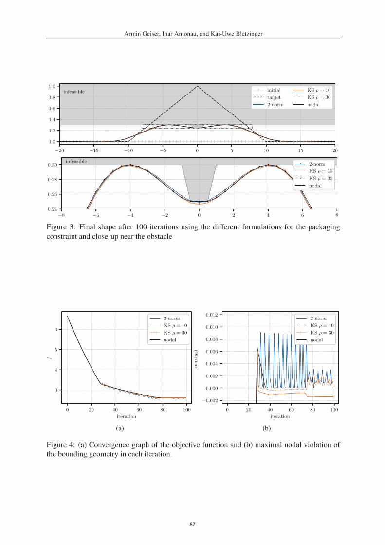
Armin Geiser, Ihar Antonau, and Kai-Uwe Bletzinger
−20 −15 −10 −5 0 5 10 15 20
0.0
0.2
0.4
0.6
0.8
1.0infeasible initial
target
2-norm
KS ρ = 10
KS ρ = 30
nodal
−8 −6 −4 −2 0 2 4 6 80.24
0.26
0.28
0.30infeasible
2-norm
KS ρ = 10
KS ρ = 30
nodal
Figure 3: Final shape after 100 iterations using the different formulations for the packaging
constraint and close-up near the obstacle
0 20 40 60 80 100
iteration
3
4
5
6
f
2-norm
KS ρ = 10
KS ρ = 30
nodal
(a)
0 20 40 60 80 100
iteration
−0.002
0.000
0.002
0.004
0.006
0.008
0.010
0.012
max(g
i)
2-norm
KS ρ = 10
KS ρ = 30
nodal
(b)
Figure 4: (a) Convergence graph of the objective function and (b) maximal nodal violation of
the bounding geometry in each iteration.
87

Armin Geiser, Ihar Antonau, and Kai-Uwe Bletzinger
geometry at a height of 0.3. From this point, the maximum nodal violation jumps between the
different geometric locations of the contact points with the packaging geometry. The aggregated
constraint stays active all the time, however, individual nodes still oscillate between feasible and
infeasible domains. The overall maximum violation does not vanish even after many iterations,
however, it remains bounded by the step size.
The case with Kreisselmeier-Steinhausser aggregation with ρ=30 shows no oscillations until
iteration 60, where the shape hits the packaging geometry at tree locations. From this point,
oscillations of the maximum nodal violation are observed, similar to the case with the 2-norm
aggregation. This can be explained by the fact, that high ρ values result in a good approxi-
mation of the maximum value. The gradient of the aggregated constraint is dominated by the
gradient of the node with the maximum violation, and even if all other nodes still contribute,
they are underrepresented, and the computed shape update might push them to the infeasible do-
main. The smaller value for ρ=10 in the Kreisselmeier-Steinhausser aggregation leads to a more
conservative approximation of the maximum violation. The contribution of the nodes to the ag-
gregated response value and gradient is more evenly distributed and relaxes the zig-zagging
behavior. This comes with a price, the approximation is too conservative and the design ge-
ometry is constrained with a distance to the packaging geometry. An optimal choice of ρ is
problem-dependent, since the number of design variables and therefore nodal constraints, and
the number of nodes that come close to the boundary affect the behavior.
The reference solution with the nodal constraints does not show any oscillatory behavior and
the packaging constraint is satisfied exactly.
In general, all four cases satisfy the geometric constraint, with small violations for the ag-
gregation with the 2-norm and the Kreisselmeier-Steinhausser function with ρ=30. Such small
violations of geometric constraints are often acceptable, especially if Vertex Morphing is used
to find new shapes in early design stages.
5 STRUCTURAL OPTIMIZATION EXAMPLE
As a second application example, we present a structural optimization of a solid hook model.
The hook has a height of 237 mm and is modeled with a linear elastic material with a Young’s
modulus E=206.9 GPa and a Poisson’s ratio ν=0.29. The mass of to hook should be minimized
while maintaining the initial compliance for two static load cases with a load at the center (LC1:
F=32 kN) and tip (LC2: F=16 kN) respectively. For both load cases, the hook is supported at
the top. In addition to the structural constraints, two geometric constraints from the previous
sections are applied. The design space is limited by a curved packaging geometry with 4505
nodes, and a minimum thickness constraint of tmin=15.0 mm. The load application area and
the supports are excluded from the shape optimization, this leads to a total number of 7117
surface nodes in the design area. A smooth transition is enforced between design and non-design
regions. The setup of the optimization problem with the initial shape and discretization of hook
and packaging geometry is shown in Figure 5. A filter radius of r=25.0 mm is used for the
Vertex Morphing parameterization, the maximum step length in search direction and correction
is limited to 1.0 mm. The shape optimization, including the adjoint sensitivity analysis of the
structural response functions and the pseudo-elastic mesh motion for the internal nodes, is done
with the ShapeOptimization-, StructuralMechanics-, and MeshMovingApplication of the open-
source software Kratos-Multiphysics [25]. The optimization is stopped after 100 iterations.
Three cases of the optimization problem are solved, comparing the different formulations for
the geometric constraints:
88

Armin Geiser, Ihar Antonau, and Kai-Uwe Bletzinger
Figure 5: Optimization setup of the hook with the load-cases, the design surface (blue), the
packaging geometry (yellow) and the simulation meshes.
0 20 40 60 80 100
iteration
−12.5
−10.0
−7.5
−5.0
−2.5
0.0
Δf[%
]
mass
2-norm
KS
nodal
0 20 40 60 80 100
iteration
−0.005
0.000
0.005
0.010
0.015
0.020
0.025
Δg[%
]
compliance
LC1: 2-norm
LC1: KS
LC1: nodal
LC2: 2-norm
LC2: KS
LC2: nodal
Figure 6: Improvement of mass objective and violation of the compliance constraints for the
three cases during the optimization process.
• 2-norm aggregation: g2-norm ≤ 0
• Kreisselmeier-Steinhausser: gKS(ρ = 18) ≤ 0
• nodal constraints: gi ≤ 0 for i = 1 . . . n nodes
The shape optimization converges to very similar shapes for all three cases, with a mass
reduction of ≈13%. The case with the Kreisselmeier-Steinhausser function leads to a bit less
improvement due to the conservative approximation of the maximum nodal violation for the
geometric constraints (Figure 6 left). Even though the aggregated geometric constraints cause
slight oscillations for the objective and the compliance constraints, the overall trend is compa-
rable to the case with node-wise constraints. The structural constraints are active during the
whole optimization, they are violated by less than 0.005% (Figure 6 right) for all three cases,
which is negligible.
Figure 7 shows the maximum nodal violation of the packaging constraint and the minimum
thickness constraint respectively for the three cases. The 2-norm aggregation again leads to a
89

Armin Geiser, Ihar Antonau, and Kai-Uwe Bletzinger
0 20 40 60 80 100
iteration
−0.50
−0.25
0.00
0.25
0.50
0.75
1.00
max(g
i)[m
m]
packaging
2-norm KS nodal
0 20 40 60 80 100
iteration
−0.50
−0.25
0.00
0.25
0.50
0.75
1.00
max(g
i)[m
m]
thickness
2-norm KS nodal
Figure 7: Maximum value of all nodal violations of packaging and thickness constraints for
the three cases during the optimization process. The violations remain much smaller then the
applied step size.
Figure 8: Final shape of the hook for the three cases, from left to right: 2-norm aggregation,
Kreisselmeier-Steinhausser aggregation, nodal constraints. The nodal violation of the packag-
ing constraint is colored, feasible nodes are colorless.
90

Armin Geiser, Ihar Antonau, and Kai-Uwe Bletzinger
Figure 9: Final shape of the hook optimization showing the nodal violation of the thickness
constraint. Feasible nodes are colorless. In the right figure, the initial (black) and geometrically
unconstrained final shape (red) are indicated.
zig-zagging behavior of the nodal violation and finally results in a maximum violation of ≈0.2
mm of both geometric constraints. Individual nodes that violate the constraint are pushed to
the feasible domain by the correction step after one iteration. Those nodes do not contribute to
the aggregated constraint gradient anymore and jump to the infeasible domain in the following
iteration. The maximum nodal value gi does not occur at the same node in each iteration. The
Kreisselmeier-Steinhausser formulation is able to satisfy the geometric constraint with slightly
smaller oscillations but is more conservative. The design surface is stopped within a distance of
≈0.2 mm to the packaging geometry and ≈0.1 mm to the minimum thickness constraint. This
leads to a slightly smaller objective improvement for this case. With another choice of ρ this
might be improved, however, i.e. ρ=25 already leads to much larger oscillations. The case with
the nodal formulation is again able to satisfy the packaging and also the minimum thickness
constraints exactly, as expected. The final shapes with the nodal violations of the packaging
constraint are shown in Figure 8. The nodal violations of the thickness constraint are shown in
Figure 9.
This example demonstrates that aggregation of geometric constraints can be applied also in
more complex shape optimization problems when other physical constraints have to be consid-
ered. The maximum number of simultaneously active constraints in this example is 173 for the
node-wise constraints and 4 for the aggregated formulations. Even though the aggregation of the
geometric constraints does amplify the known zig-zagging behavior of the gradient-projection
algorithm, the negative impact on the objective improvement and enforcement of the physical
constraints is negligible. It is highlighted that globally the same shapes are found in all three
cases.
91

Armin Geiser, Ihar Antonau, and Kai-Uwe Bletzinger
6 CONCLUSIONS
Constraint aggregation functions have been successfully applied to geometric constraints
in shape optimization problems with the Vertex Morphing parameterization and a gradient-
projection algorithm. The performance of the aggregation functions has been evaluated in an
academic 1D example and a 3D structural-mechanics example, comparing with the node-wise
application of the constraints. The latter example was also subject to additional structural con-
straints. The overall number of constraints can be drastically reduced, which is of interest,
especially for large models. With both investigated constraint aggregation functions, the same
shapes as are found as with the reference solution with nodal geometric constraints. Depend-
ing on the aggregation formulation, the final shape does either slightly violate the geometric
constraint, or is stopped within a small distance to the constraint limit in case of a conserva-
tive choice of the ρ value of the Kreisselmeier-Steinhausser formulation. Such small deviations
from the geometric constraints are often acceptable when searching new shapes, and constraint
aggregation can be an efficient alternative to the numerically challenging nodal application of
the constraints.
ACKNOWLEDGEMENT
This work has been carried out within the MADELEINE project which has received fund-
ing from the European Union’s Horizon 2020 research and innovation programme under grant
agreement N 769025.
References
[1] Shenren Xu, Wolfram Jahn, and Jens-Dominik Muller. CAD-based shape optimisation
with CFD using a discrete adjoint. International Journal for Numerical Methods in Fluids,
74(3):153–168, 2014. ISSN 1097-0363. doi: 10.1002/fld.3844.
[2] J. Kiendl, R. Schmidt, R. Wuchner, and K.-U. Bletzinger. Isogeometric shape optimiza-
tion of shells using semi-analytical sensitivity analysis and sensitivity weighting. Com-puter Methods in Applied Mechanics and Engineering, 274:148–167, June 2014. ISSN
00457825. doi: 10.1016/j.cma.2014.02.001.
[3] Antony Jameson. Optimum aerodynamic design using CFD and control theory. In 12thComputational Fluid Dynamics Conference, San Diego,CA,U.S.A., June 1995. American
Institute of Aeronautics and Astronautics. doi: 10.2514/6.1995-1729.
[4] Hideyuki Azegami and Kenzen Takeuchi. A smoothing method for shape optimiza-
tion: Traction method using the Robin condition. International Journal of Compu-tational Methods, 03(01):21–33, March 2006. ISSN 0219-8762, 1793-6969. doi:
10.1142/S0219876206000709.
[5] Chau Le, Tyler Bruns, and Daniel Tortorelli. A gradient-based, parameter-free approach
to shape optimization. Computer Methods in Applied Mechanics and Engineering, 200
(9-12):985–996, February 2011. ISSN 00457825. doi: 10.1016/j.cma.2010.10.004.
[6] Stefan Riehl, Jan Friederich, Michael Scherer, Ralf Meske, and Paul Steinmann. On
the discrete variant of the traction method in parameter-free shape optimization. Com-puter Methods in Applied Mechanics and Engineering, 278:119–144, August 2014. ISSN
00457825. doi: 10.1016/j.cma.2014.05.009.
92
Armin Geiser, Ihar Antonau, and Kai-Uwe Bletzinger
[7] Matthias Firl and Kai-Uwe Bletzinger. Shape optimization of thin walled structures
governed by geometrically nonlinear mechanics. Computer Methods in Applied Me-chanics and Engineering, 237-240:107–117, September 2012. ISSN 0045-7825. doi:
10.1016/j.cma.2012.05.016.
[8] Gregoire Allaire, Francois Jouve, and Anca-Maria Toader. A level-set method for shape
optimization. Comptes Rendus Mathematique, 334(12):1125–1130, January 2002. ISSN
1631-073X. doi: 10.1016/S1631-073X(02)02412-3.
[9] Kai-Uwe Bletzinger. A consistent frame for sensitivity filtering and the vertex assigned
morphing of optimal shape. Structural and Multidisciplinary Optimization, 49(6):873–
895, June 2014. ISSN 1615-147X, 1615-1488. doi: 10.1007/s00158-013-1031-5.
[10] Majid Hojjat, Electra Stavropoulou, and Kai-Uwe Bletzinger. The Vertex Morphing
method for node-based shape optimization. Computer Methods in Applied Mechanicsand Engineering, 268:494–513, January 2014. ISSN 00457825. doi: 10.1016/j.cma.2013.
10.015.
[11] Kai-Uwe Bletzinger. Shape Optimization. In Erwin Stein, Rene de Borst, and Thomas
J R Hughes, editors, Encyclopedia of Computational Mechanics Second Edition, pages 1–
42. John Wiley & Sons, Ltd, Chichester, UK, December 2017. ISBN 978-1-119-00379-3
978-1-119-17681-7. doi: 10.1002/9781119176817.ecm2109.
[12] Oliver Schmitt, Jan Friederich, Stefan Riehl, and Paul Steinmann. On the formulation
and implementation of geometric and manufacturing constraints in node–based shape op-
timization. Structural and Multidisciplinary Optimization, 53(4):881–892, April 2016.
ISSN 1615-1488. doi: 10.1007/s00158-015-1359-0.
[13] G. Allaire, F. Jouve, and G. Michailidis. Thickness control in structural optimization via a
level set method. Structural and Multidisciplinary Optimization, 53(6):1349–1382, June
2016. ISSN 1615-1488. doi: 10.1007/s00158-016-1453-y.
[14] Oliver Schmitt and Paul Steinmann. Control of minimum member size in parameter-
free structural shape optimization by a medial axis approximation. Computational Me-chanics, 61(6):717–727, June 2018. ISSN 0178-7675, 1432-0924. doi: 10.1007/
s00466-017-1477-1.
[15] Reza Najian Asl, Shahrokh Shayegan, Armin Geiser, Majid Hojjat, and Kai-Uwe Blet-
zinger. A consistent formulation for imposing packaging constraints in shape opti-
mization using Vertex Morphing parametrization. Structural and Multidisciplinary Op-timization, 56(6):1507–1519, December 2017. ISSN 1615-147X, 1615-1488. doi:
10.1007/s00158-017-1819-9.
[16] Benjamin J. Brelje, Joshua L. Anibal, Anil Yildirim, Charles A. Mader, and Joaquim R.
R. A. Martins. Flexible Formulation of Spatial Integration Constraints in Aerodynamic
Shape Optimization. AIAA Journal, 58(6):2571–2580, May 2020. ISSN 0001-1452. doi:
10.2514/1.J058366.
[17] Marios Damigos, E. Papoutsis-Kiachagias, and Kyriakos Giannakoglou. Adjoint Variable-
based Shape Optimization with Bounding Surface Constraints. International Journal forNumerical Methods in Fluids, 93, July 2020. doi: 10.1002/fld.4900.
93

Armin Geiser, Ihar Antonau, and Kai-Uwe Bletzinger
[18] J. B. Rosen. The Gradient Projection Method for Nonlinear Programming. Part I. Linear
Constraints. Journal of the Society for Industrial and Applied Mathematics, 8(1):181–217,
March 1960. ISSN 0368-4245, 2168-3484. doi: 10.1137/0108011.
[19] J. B. Rosen. The Gradient Projection Method for Nonlinear Programming. Part II. Non-
linear Constraints. Journal of the Society for Industrial and Applied Mathematics, 9(4):
514–532, December 1961. ISSN 0368-4245. doi: 10.1137/0109044.
[20] Raphael T. Haftka and Zafer Gurdal. Constrained Optimization. In Raphael T. Haftka
and Zafer Gurdal, editors, Elements of Structural Optimization, Solid Mechanics And Its
Applications, pages 159–207. Springer Netherlands, Dordrecht, 1992. ISBN 978-94-011-
2550-5. doi: 10.1007/978-94-011-2550-5 5.
[21] Long Chen, Kai-Uwe Bletzinger, Armin Geiser, and Roland Wuchner. A modified search
direction method for inequality constrained optimization problems using the singular-
value decomposition of normalized response gradients. Structural and MultidisciplinaryOptimization, 60(6):2305–2323, December 2019. ISSN 1615-147X, 1615-1488. doi:
10.1007/s00158-019-02320-9.
[22] Ihar Antonau, Majid Hojjat, and Kai-Uwe Bletzinger. Relaxed gradient projection
algorithm for constrained node-based shape optimization. Structural and Multidisci-plinary Optimization, February 2021. ISSN 1615-147X, 1615-1488. doi: 10.1007/
s00158-020-02821-y.
[23] Andrew B. Lambe, Graeme J. Kennedy, and Joaquim R. R. A. Martins. An evaluation of
constraint aggregation strategies for wing box mass minimization. Structural and Multi-disciplinary Optimization, 55(1):257–277, January 2017. ISSN 1615-147X, 1615-1488.
doi: 10.1007/s00158-016-1495-1.
[24] G. Kreisselmeier and R. Steinhauser. Systematic Control Design by Optimizing a Vector
Performance Index. IFAC Proceedings Volumes, 12(7):113–117, September 1979. ISSN
1474-6670. doi: 10.1016/S1474-6670(17)65584-8.
[25] Vicente Mataix Ferrandiz, Philipp Bucher, Riccardo Rossi, Ruben Zorrilla, Jordi Cotela,
Josep Maria, Miguel Angel Celigueta, and Guillermo Casas. KratosMultiphysics/Kratos:
KratosMultiphysics 8.1. Zenodo, November 2020.
94

AN OPTIMIZATION ALGORITHM FOR THE DETECTION OF DAMAGE IN FRAME STRUCTURES
Annalisa Greco 1, Ilaria Fiore 1, Alessandro Pluchino 2
1 Department of Civil Engineering and Architecture, University of Catania via S. Sofia 64, Catania, Italy
[email protected], [email protected]
2 Department of Physics and Astronomy “Ettore Majorana”, University of Catania, and INFN, Unit of Catania, via S. Sofia 64, Catania, Italy
Abstract
The aim of the study is the formulation of a computational method for the identification of the first damage in planar frames. The damage is considered to be concentrated in some oppor-tune sections of beams and columns and many assume different intensities. In order to identify the location and intensity of the damage when measured frequencies on the damaged frame are available, an original algorithm has been implemented assigning to each critical section an appropriate fitness function. This function indicates the difference be-tween the measured frequencies of vibration and those obtained, by means of opportune nu-merical models, assuming that the damage is located in the considered critical section. The exact location will then be individuated seeking the optimal fitness function. An iterative pro-cedure which allows reducing the computational effort is also presented with reference to a case study.
Keywords: Damage identification; Frames; Stiffness matrix; Frequencies of vibration.
95

Annalisa Greco, Ilaria Fiore and Alessandro Pluchino
1 INTRODUCTION
As it can be observed from the scientific literature of recent decades, structural health mon-itoring of existing structures has received great interest and has inspired many dedicated stud-ies. Many studies are devoted to the evaluation of the static or dynamic response of damaged structures and highlight their modification with respect to undamaged configurations [1-9]. The presence of structural damage reduces the bearing capacity of structures and therefore, in order to prevent its progressive expansion, which inevitably leads to structural failure, must be detected in its early stage. Many damage identification techniques are reported in the literature and require the measurement of some data on the existing structure. Different data can be tak-en into account for instance the variation of dynamic characteristics, such as natural frequen-cies [10-17], mode shapes [18,19], or static quantities, such as displacements or strains induced by applied loads [20-22]. Many studies are based on the solution of an inverse prob-lem that compares numerical response data, evaluated on a model of the structure, to the cor-responding experimentally measured ones [23-25]. Recent computational procedures based on genetic algorithms [26-28], particle swarm optimization [29], fuzzy cognitive maps [30] have been presented.
A crucial aspect concerns the model of damage and numerous attempts to quantify local defects are reported in the literature. All the models involve a reduction of the stiffness of the structural element by using one-dimensional continuum theories [31] or fracture mechanics methods [32,33].
The damage can be either localized or diffused on a certain portion of the length of the structural element and its intensity can be related to the reduction of the reactive area of the cross section, for example due to the presence of a notch. Contributions on crack modelling approaches and their effects on the response of beams can be found in [34,35].
The aim of the present paper is to propose a computational method for monitoring the structural integrity of planar frames. It is assumed that appropriate sensors are permanently located on the frame detecting its vibration properties with a certain periodicity. In this case it will be possible to immediately detect the appearance of the first structural damage indicated by a difference between some measured data and those known for the undamaged frame. The widely used assumption of a hinge with a rotational spring is used to model the damage and this is assumed to be concentrated, located in opportune critical sections and may have differ-ent intensities.
With the aim of identifying the location of the first damage, the frequencies of vibration of undamaged and damaged frames are calculated. In particular the frequencies of vibration are evaluated for each damage configuration of the frame corresponding to a possible location of damage among the considered critical sections. These frequencies of vibration are then used to identify the location and the intensity of the damage by means of the solution of an oppor-tune optimization problem. The application on a case study allows to show the reliability of the proposed identification algorithm. Furthermore, an automatic procedure is illustrated which, assigning to each critical section an opportune fitness with respect to the possibility that the damage is located there, allows to iteratively converge to the exact position reducing the required computational effort.
2 FREQUENCIES OF VIBRATION IN UNDAMAGED AND DAMAGED FRAMES
In the present study planar regular frames, with columns clamped at the ground level, are considered. Once the mechanical and geometrical characteristics of each structural member of the frame have been assigned, the stiffness and mass matrices of the undamaged frame respec-tively denoted as Ku and Mu can be evaluated. In particular the mass matrix takes into account
96

Annalisa Greco, Ilaria Fiore and Alessandro Pluchino
of the distributed masses in beams and columns. Neglecting the axial deformability of the structural members, the degrees of freedom of the frame, and therefore the size of the stiffness and mass matrices, correspond to the horizontal displacements of each floor and the rotation of the unconstrained nodes. The natural frequencies of vibration u of the undamaged frame can be evaluated solving the classic equation:
( )2det 0u uuω− =K M (1)
When the first damage occurs in a structural member the total stiffness decreases and con-sequently also the frequencies of vibration assume lower values with respect to the undam-aged configuration.
In this study reference is made to a single damage which can be located in one of the criti-cal sections of the frame corresponding to the base or top of each column at each floor or to the ends of each beam. With reference to the two corners at the top of the frame, the critical section will be located in correspondence to the structural member (beam or column) having the lower elastic moment.
In accordance with what is frequently adopted in the scientific community, the loss of re-sistance induced by the presence of the damage is modelled by means of a hinge with a rota-tional spring whose stiffness kϕ is related to the intensity of the damage.
In order to evaluate the natural frequencies of the frame having a damage located in one of the previously described critical sections, new stiffness and mass matrices must be assembled. For each location of the damage, stiffness and mass matrices, respectively denoted as Kd and Md
, are evaluated. The correspondent frequencies of vibration for each location of the dam-age are evaluated solving the equation:
( )2det 0d ddω− =K M (2)
The stiffness of the rotational spring modelling the damage will be assumed equal to ni dis-crete values which decrease with the intensity of the damage itself. In particular, the stiffness of the rotational spring is expressed as:
1, ... ,di i i
d
EIk i n
Lϕ α= = (3)
where αi is an integer number and Id and Ld are respectively the moment of inertia and thelength of the structural element where the damage is located (beam or column).
3 DAMAGE IDENTIFICATION PROCEDURE
In this section the damage parameters, i.e. location and intensity, are evaluated by means of an optimization strategy based on the use of a certain number of vibration properties meas-ured on the considered frame. For each possible damage location among the critical sections a fitness value is assigned for each damage intensity as follows:
,, max
ˆ1, ... ,
nfi i kj
k j ii iu
F F j nω ω
ω−
= − = (4)
where:
Fmax is an arbitrary constant, chosen great enough to have always Fk > 0 nf is the number of considered natural frequencies
97

Annalisa Greco, Ilaria Fiore and Alessandro Pluchino
ni is the number of considered damage intensities ˆ
iω is the measured i-th frequency of vibration
,i kjω is the calculated i-th frequency of vibration with intensity damage j located in critical
section k
iuω is the i-th frequency of vibration for the undamaged frame
For each critical section the maximum fitness among those associated to different intensity values is then selected:
( ),max 1, ... ,k k j iF F j n= = (5)
Of course, among all the fitness functions associated to possible damage locations, only the one related to the exact position will reach its maximum value.
Once the position of the damage is identified, it is possible to evaluate its intensity compar-ing all the sets of frequencies related to variable intensity to the measured values.
The first step of the proposed algorithm concerns with the localization of the damaged sec-tion and represents the main goal of the proposed approach. Undoubtably from a health moni-toring point of view the most crucial aspect is to identify the presence and the location of the damage. Once the damage is detected it is important to repair as soon as possible the involved structural zones in order to prevent subsequent worsening, independently on the damage in-tensity.
In principle all the natural frequencies of all the possible configurations of damaged frames can be calculated and the correct location of the damage can be identified minimizing the fit-ness function. Anyway, it will be shown that it is sufficient to take into account only some natural frequencies in order to identify the correct damage location. In the applicative section the number of considered frequencies of vibration has been set equal to 4. For large frames with high number of critical sections in order to reduce the number of calculated fitness val-ues, an original iterative procedure described in the following can be applied.
It is worth pointing out that the proposed procedure applies both for damage identification in symmetric and unsymmetric frames. Anyway, in case of symmetric frames it is not possi-ble to discern between symmetric damage positions. However, in order to carry out mainte-nance and restoration interventions, this circumstance does not appear to be a major limitation as it allows to drastically reduce the sections to be considered to two only. Anyway, if one needs to univocally identify the damaged section in a symmetric frame, some information on mode shapes could be added in the objective function.
4 CASE STUDY AND NUMERICAL APPLICATIONS
The five storeys frame assumed as case study for the proposed damage identification pro-cedure is shown in Figure 1. In the same figure the length and the profiles of the structural members are also reported. In Table 1 moments of inertia and the ratio between yield mo-ments of the cross sections and the yield stress are reported together with the values of the dis-tributed masses. The value of Young modulus for the steel under consideration is assumed to
be: 2
210000000kN
Em
=
98

Annalisa Greco, Ilaria Fiore and Alessandro Pluchino
3.5 [m]
5 [m]
3 [m]
HE 240 A
HE 200 A
3.5 [m]
HE 240 A
4 [m]
HE 240 A
4.5 [m]
HE 280 A
5 [m]
3.5 [m]
4 [m]
HE 240 A
HE 280 A
HE 320 A
HE 200 A
HE 240 A
Figure 1 - Frame with five floors and four columns
Profile Ix [m4] My /σy[m3] m [kN*s2/m2] HE320A 22930 10-8 1479 10-6 97.6 10-3 HE280A 13670 10-8 1013 10-6 76.4 10-3 HE240A 7763 10-8 675.1 10-6 60.3 10-3 HE200A 3692 10-8 388.6 10-6 42.3 10-3
Table 1 - Characteristics of the structural elements
For this frame the numbers of degrees of freedom in the undamaged configuration is equal to 30 and therefore 30 frequencies of vibration can be calculated solving the related dynamic eigenvalue problem once the matrices Ku and Mu are evaluated.
The total number of critical sections for the considered frame is 88 but since it is symmet-ric, 49 critical sections must be taken into account. For each possible location of the damage, and for each value of its intensity, 31 frequencies of vibration can be calculated. Considering, eight levels of intensity of the damage, 392 sets of 31 frequencies of vibration have been evaluated. With the aim of solving the inverse problem which concerns the identification of damage parameters, some examples of location and intensity of the damage will be developed, and the related natural frequencies will be used as pseudo-experimental data in the identifica-tion procedure.
4.1 The Identification Algorithm
The identification algorithm has been realized within the software environment NetLogo [36], where the five storey frame can be reproduced in a virtual metric space, as shown in panel (a) of Figure 2. The critical sections Sk (k = 1,…,88), represented by yellow squares, are labeled with an increasing ID number. Among them, let us call ST the target (damaged) sec-tion.
99
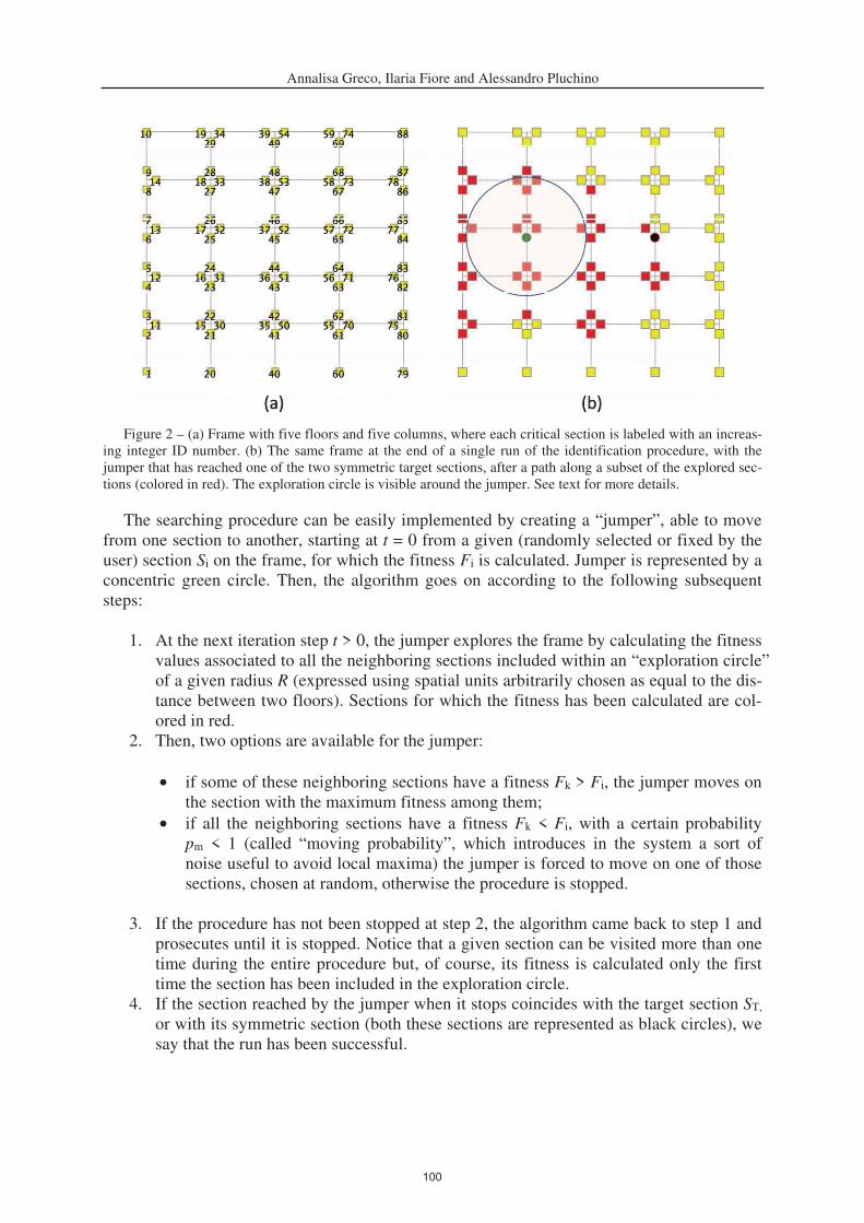
Annalisa Greco, Ilaria Fiore and Alessandro Pluchino
Figure 2 – (a) Frame with five floors and five columns, where each critical section is labeled with an increas-ing integer ID number. (b) The same frame at the end of a single run of the identification procedure, with the jumper that has reached one of the two symmetric target sections, after a path along a subset of the explored sec-tions (colored in red). The exploration circle is visible around the jumper. See text for more details.
The searching procedure can be easily implemented by creating a “jumper”, able to move from one section to another, starting at t = 0 from a given (randomly selected or fixed by the user) section Si on the frame, for which the fitness Fi is calculated. Jumper is represented by a concentric green circle. Then, the algorithm goes on according to the following subsequent steps:
1. At the next iteration step t > 0, the jumper explores the frame by calculating the fitnessvalues associated to all the neighboring sections included within an “exploration circle”of a given radius R (expressed using spatial units arbitrarily chosen as equal to the dis-tance between two floors). Sections for which the fitness has been calculated are col-ored in red.
2. Then, two options are available for the jumper:
• if some of these neighboring sections have a fitness Fk > Fi, the jumper moves onthe section with the maximum fitness among them;
• if all the neighboring sections have a fitness Fk < Fi, with a certain probabilitypm < 1 (called “moving probability”, which introduces in the system a sort ofnoise useful to avoid local maxima) the jumper is forced to move on one of thosesections, chosen at random, otherwise the procedure is stopped.
3. If the procedure has not been stopped at step 2, the algorithm came back to step 1 andprosecutes until it is stopped. Notice that a given section can be visited more than onetime during the entire procedure but, of course, its fitness is calculated only the firsttime the section has been included in the exploration circle.
4. If the section reached by the jumper when it stops coincides with the target section ST,
or with its symmetric section (both these sections are represented as black circles), wesay that the run has been successful.
100

Annalisa Greco, Ilaria Fiore and Alessandro Pluchino
In panel (b) of Figure 2 the situation at the end of a generic successful run is reported, with the jumper over the target. An example of exploration circle, centered on the jumper, is also shown for allowing the user to visualize it. The percentage E% of explored (red) sections over the total is visibly around 50% and this tell us that the algorithm was not only effective (since the jumper reached the target) but also efficient, since we were able to identify the damaged section without needing to calculate the fitness for all the sections.
Of course, in order to have more reliable information about the effectiveness and the effi-ciency of the proposed algorithm for the identification of a given (fixed) target section, one needs to repeat N times (with N >> 1) the entire procedure starting, for each run, from a dif-ferent random section. At the end of the N repetitions, the percentage P% of successful runs and the average percentage E% of explored sections will represent the quantities that we have to take into account for evaluating the performance of the algorithm.
4.2 Results for the five storeys frame
In this paragraph we discuss the numerical results obtained by applying our algorithm to the considered five storeys frame. The damage can be located in each of the 49 critical sec-tions and eight damage intensities, represented by the rotational stiffness given by equation (3) with [ ]1000 800 700 500 300 100 50 25α = , have been taken into account.
Considering different arbitrary sets of location and intensity of the damage and assuming the correspondent first four frequencies of vibration as pseudo-experimental data, the fitness function (4) has been previously evaluated for each of the 49 critical sections observing that it always reached a zero value in correspondence of the exact damage configuration.
Successively in order to implement the searching procedure described in the previous sec-tion (and therefore to avoid the calculation of the fitness for all the sections), the two percent-ages P% (of successful runs) and E% (of explored sections) have been evaluated assuming different damage locations and intensities.
In order to evaluate an appropriate value of the radius of the exploration able to provide re-liable results still maintaining a significant reduction in the number of nodes in which the fit-ness function has to be calculated, a preliminary analysis has been developed. Figure 3 shows the results obtained assuming for example the damage located in sections 1 and 15 (involving respectively one column and one beam) with intensity 300α = and evaluating the two per-centages P% and E% for increasing values of R. As it can be observed, increasing the value of the radius, higher values of both P% and E% are reached. A fair compromise between the need of reaching high values of P% without increasing too much E% can be obtained assuming R=2,2, so this value will be chosen for the simulations. Figure 4 shows the effect of the forc-ing moving probability pm in the identification of the damage located again in sections 1 and 15 with intensity 300α = . While for the damage located on the beam the two percentages P%
and E% show to be almost independent on pm, for the damaged column a sensible increase with the forcing moving probability can be observed. In order to choose a unique value, in the following pm has been set equal to 0,9.
With the aim of investigating on the effects of a damage located at the base of a column or on a beam at each floor, the sections 1, 3, 5, 7, 9 (base columns) and 15, 16, 17, 18, 19 (right end of beams of the first span) have been taken into account. Several sets of N = 1000 runs have been performed and the results in terms of P% and E% have been reported in Figure 5.
101

Annalisa Greco, Ilaria Fiore and Alessandro Pluchino
Figure 3 – P% and E% for damage located at the base of a column (1) and on a beam (15) of the first floor with stiffness intensity parameter =300 for different values of the radius parameter
Figure 4 – P% and E% for damage located at the base of a column (1) and on a beam (15) of the first floor with stiffness intensity parameter =300 for different values of the forcing moving probability
As it can be observed from Figure 5 the damage identification procedure gives excellent results when the damage is located on one of the considered beams. In these cases, in fact, independently on the considered section (and therefore on the floor) the percentage of suc-cessful runs turns out to be always 100% while the percentage of explored sections is about 80%. On the other hand, the identification of damages located at the base of the external col-umns provide values of P% around 85% with E% always smaller than 60%
Therefore, we can conclude that, for the considered five storeys frame, the proposed identi-fication procedure provided satisfactory results, thus confirming its good performance and reliability.
5 CONCLUSIONS
• A computational method for monitoring the structural integrity of planar frames is pre-sented.
• The first damage is identified by means of the frequencies of vibration of each damagedconfiguration of the frame corresponding to a possible location of damage among theconsidered critical sections.
• The solution of the damage identification problem is achieved by means of an optimiza-tion algorithm which assigns to each possible damage location, among the critical sec-tions, a fitness value and then seeks the maximum one.
102

Annalisa Greco, Ilaria Fiore and Alessandro Pluchino
Figure 5 – P% and E% for assigned damage location and variable intensity Left side: damage located at the base of an external column at each floor starting from the base
Right side: damage located at the right end of each beam in the first bay starting from the bottom
103

Annalisa Greco, Ilaria Fiore and Alessandro Pluchino
• An automatic procedure has been implemented within the software environmentNetLogo and it has been shown how it is possible to iteratively converge to the exactdamage position reducing the number of calculations.
• The application to a case study allows to show the reliability of the proposed identifica-tion algorithm.
REFERENCES
[1] T. Chondros and A. G. Dimagoronas, "Dynamic sensitivity of structures to cracks," Journal of Vibration and Acoustics, vol. 111, pp. 251-256, 1989.
[2] M.-H. Shenn and C. Pierre, "Natural modes of Bernoulli-Euler beams with symmetric cracks," Journal of Sound and Vibration, vol. 138, no. 1, pp. 115-134, 1990.
[3] W. Ostachowicz and M. Krawczuk, "Analysis of the effects of cracks on the natural frequencies of a cantilever beam," Journal of Sound and Vibration, vol. 150, no. 2, pp. 191-201, 1991.
[4] I. Caliò, D. D'Urso and A. Greco, "The influence of damage on the eigen-properties of Timoshenko spatial arches," Computers & Structures, vol. 190, pp. 13-24, 2017.
[5] B. Bozvigit, Y. Yesilce and M. Wahab, "Free vibration and harmonic response of cracked frames using a single variable shear deformation theory," Structural Engineering and Mechanics, vol. 74, no. 1, pp. 33-54, 2020.
[6] K. Mazanoglu and E. Kandemir-Mazanoglu, "A new simplified method for anti-symmetric mode in-plane vibrations of frame structures with column cracks," Journal of Vibration and Control, vol. 24, no. 24, pp. 5794-5810, 2018.
[7] U. Eroglu and E. Tufekci, "Free Vibration of Damaged Frame Structures Considering the Effects of Axial Extension, Shear Deformation and Rotatory Inertia: Exact Solution," International Journal of Structural Stability and Dynamics, vol. 17, no. 10, 2017.
[8] S. Caddemi and I. Caliò, "The exact explicit dynamic stiffness matrix of multi-cracked Euler-Bernoulli beam and applications to damaged frame structures," Journal of Sound and Vibration, vol. 332, no. 12, pp. 3049-3063, 2013.
[9] A. Ibrahim, H. Ozturk and M. Sabuncu, "Vibration analysis of cracked frame structures," Structural Engineering and Mechanics, vol. 45, no. 1, pp. 33-52, 2013.
[10] M. Cerri and F. Vestroni, "Identification of damage due to open cracks by changes of measured frequencies," in Proceedings of XVI AIMETA Congress of Theoretical and Applied Mechanics;, 2003.
[11] A. Morassi, "Structural identification of a steel frame from dynamic test-data," Structural Engineering and Mechanics, vol. 11, no. 3, pp. 237-258, 2001.
[12] F. Vestroni and D. Capecchi, "Damage detection in beam structures based on frequency measurements," Journal of Engineering Mechanics, vol. 126, pp. 761-768, 2000.
[13] A. Pau, A. Greco and F. Vestroni, "Numerical and experimental detection of concentrated damage in a parabolic arch by measured frequency variations," Journal of Vibration and Control, pp. 1-11, 2010.
[14] M. Dilena and A. Morassi, "Reconstruction method for damage detection in beams based on natural frequency and antiresonant frequency measurements," Journal of Engineering
104

Annalisa Greco, Ilaria Fiore and Alessandro Pluchino
Mechanics, vol. 136, no. 3, pp. 329-344, 2010.
[15] E. M. N. Giordano, M. Masciotta, F. Clementi, N. Sadeghi, R. Silva and D. Oliveira, "Expeditious damage index for arched structures based on dynamic identification testing," Construction and Building Materials, vol. 265, 2020.
[16] A. Labib, D. Kennedy and C. Featherston, "Crack localisation in frames using natural frequency degradations," Computers and Structures, vol. 157, pp. 51-59, 2015.
[17] L. Rubio, J. Fernández-Sáez and A. Morassi, "Identification of an open crack in a beam with variable profile by two resonant frequencies," Journal of Vibration and Control, vol. 24, no. 5, pp. 839-859, 2018.
[18] M. Diaferio and V. Sepe, "Modal identification of damaged frames," Structural Control and Health Monitoring, vol. 23, no. 1, pp. 82-102, 2016.
[19] M. Ge, E. Lui and A. Khanse, "Non-proportional damage identification in steel frames," Engineering Structures, vol. 32, no. 2, pp. 523-533, 2010.
[20] A. Greco and A. Pau, "Detection of a concentrated damage in a parabolic arch by measured static displacements," Structural Engineering and Mechanics, vol. 39, pp. 751-765, 2011.
[21] S. Caddemi and A. Greco, "The influence of instrumental errors on the static identification of damage parameters for elastic beams," Computer and Structures, vol. 84, pp. 1696-1708, 2006.
[22] J. Guo, L. Wang and I. Takewaki, "Static damage identification in beams by minimum constitutive relation error," Inverse Problems in Science and Engineering, vol. 27, no. 10, pp. 1347-1371, 2019.
[23] M. Friswell, "Damage identification using inverse methods," Philosophical Transactions of the Royal Society, vol. 365, pp. 393-410, 2007.
[24] P. Nikolakopoulos, D. Katsareas and C. Papadopoulos, "Crack identification in frame structures," Computers and Structures, vol. 64, pp. 389-406, 1997.
[25] A. Greco and A. Pau, "Damage identification in Euler frames," Computers and Structures, Vols. 92-93, pp. 328-336, 2012.
[26] A. Greco, D. D'Urso, F. Cannizzaro and A. Pluchino, "Damage identification on spatial Timoshenko arches by means of genetic algorithms," Mechanical Systems and Signal Processing, vol. 105, pp. 51-67, 2018.
[27] A. Yu, J. Ji and S. Sun, "An improved multi-objective genetic algorithm and data fusion in structural damage identification," International Journal of Security and Networks, vol. 14, no. 2, pp. 95-102, 2019.
[28] A. Greco, A. Pluchino, F. Cannizzaro, S. Caddemi and I. Caliò, "Closed-form solution based genetic algorithm software: Application to multiple cracks detection on beam structures by static tests," Applied Software Computing Journal, vol. 64, pp. 35-48, 2018.
[29] F. Kang, J.-J. Li and Q. Xu, "Damage detection based on improved particle swarm optimization using vibration data," Applied Software Computing Journal, vol. 12, no. 8, pp. 2329-2335, 2012.
[30] P. Beena and R. Ganguli, "Structural damage detection using fuzzy cognitive maps and Hebbian learning," Applied Software Computing Journal, vol. 11, no. 1, pp. 1014-1020, 2011.
[31] S. Christides and D. Barr, "One-dimensional theory of cracked Bernoulli-Euler beams," International Journal of Mechanics Science, vol. 26, no. 11-12, pp. 639-648, 1984.
105

Annalisa Greco, Ilaria Fiore and Alessandro Pluchino
[32] T. Chondros, "The continuous crack flexibility model for crack identification," Fatigue and Fracture of Engineering Materials and Structure, vol. 24, pp. 643-650, 2001.
[33] T. Chondros, A. Dimarogonas and J. Yao, "A continuous cracked beam vibration theory," Journal of Sound and Vibration, vol. 215, no. 1, pp. 17-34, 1998.
[34] A. Dimarogonas, "Vibration of cracked structures: a state of the art review," Engineering Fracture Mechanics, vol. 55, no. 5, pp. 831-857, 1996.
[35] I. Caliò, A. Greco and D. D'Urso, "Structural models for the evaluation of eigen-properties in damaged spatial arches: a critical appraisal," Archive of Applied Mechanics, vol. 86, pp. 1853-1867, 2016.
[36] Wilensky, U. (1999). NetLogo. http://ccl.northwestern.edu/netlogo/
106

SOFT COMPUTING FRAMEWORK FOR THE UNCERTAINTY-BASED OPTIMIZATION OF THE LENGTH AND HEIGHT OF OGEE-
CRESTED SPILLWAY
Jafar Jafari-Asl , Mohamed El Amine Ben Seghier ,Sima Ohadi and Vagelis Plevris
Abstract
Dams are one of the most important and biggest critical infrastructures of any country. The failure of a dam can be a major catastrophic event, causing irreparable environmental, human and financial losses. The low overflow capacity of the spillway is considered a major failure mode for dams. Generally, the design of spillways is carried out based on deterministic ap-proaches. However, there are many uncertainty factors in the design parameters, which have a crucial influence on the spillway performance. In this study, a new framework is presented for the accurate design of the spillways considering the surrounding uncertainty factors of the effective parameters on spillway failure causes. Therefore, the length and height of an ogee-crested spillway is considered as the design variables to be optimized. For this purpose, a meta-heuristic algorithm based on machine learning techniques is used. This latter consists of the grey wolf optimizer (GWO), while the combination of GWO and the Monte Carlo simulation (MCS) with the Kriging meta-model are utilized as a new framework for the optimum design of spillway under uncertainties. The proposed framework is investigated on the spillway redesign of a real case study in Iran.
Keywords:
107

1 INTRODUCTION
2 PROBLEM FORMULATION
108

Objective function:
Constraints:
CPI L P
Q
C HL P
H
X
3 PROPOSED METHODOLOGY
L PH
3.1 Grey wolf optimizer (GWO)
109

α β δω
α β δ
XX pXX
t AA DDD
aa rr rr
aa
3.2 Kriging (KR)
G X
f X β f Xβ S X n
Xi i n Yn
R n n
110

3.3 Monte Carlo Simulation (MCS)
G X
N I X X X
111

4 APPLICATION AND RESULTS
4.1 Case study
Component Quantity
4.2 Results and discussion
MAPE SDR
112

i i i
n
RR
R
Model MAPE SD R2
113
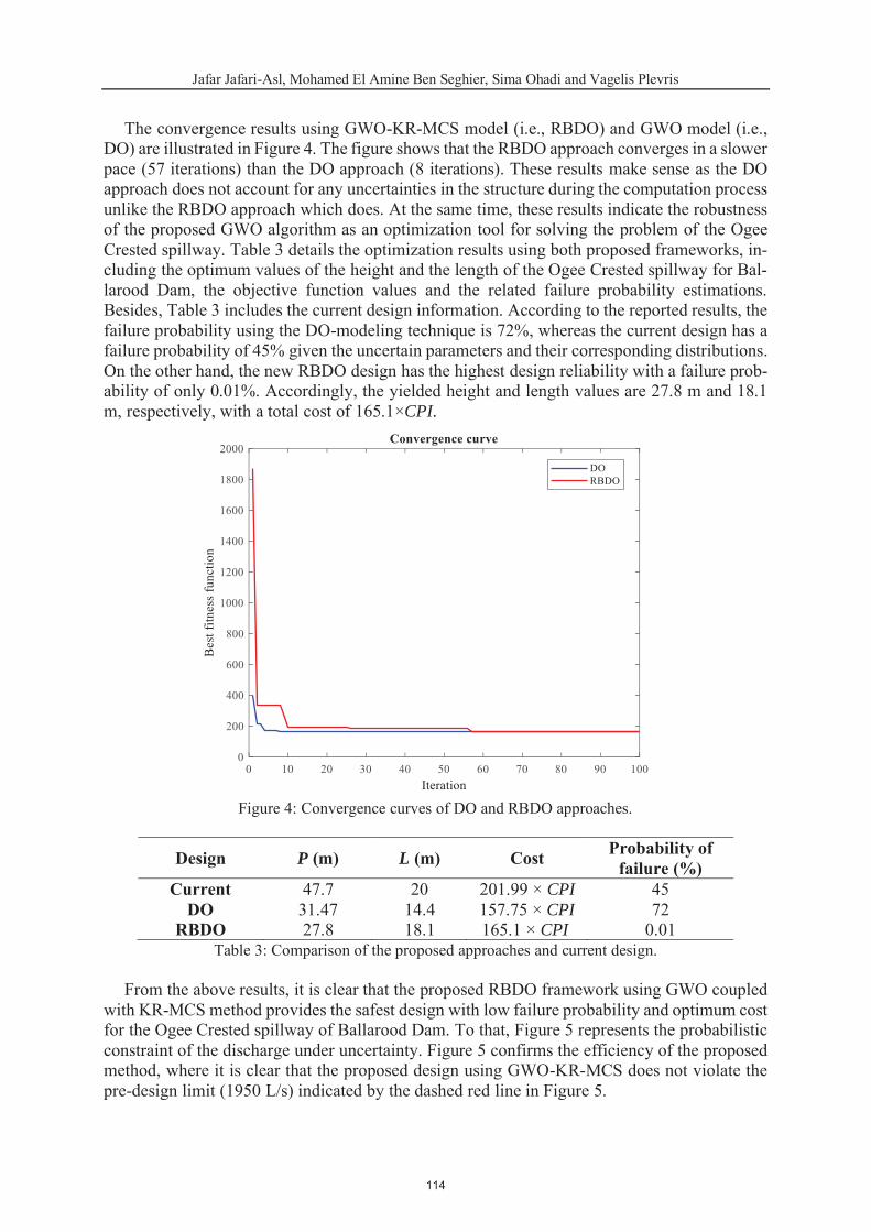
CPI.
Design P (m) L (m) Cost Probability of failure (%)
Current CPIDO CPI
RBDO CPI
114

5 CONCLUSIONS
R
115

REFERENCES
y‐
116

:
117

DESIGN OF REINFORCED CONCRETE ISOLATED FOOTINGS UNDER AXIAL LOADING WITH ARTIFICIAL NEURAL NETWORKS
German Solorzano and Vagelis Plevris
Abstract
In engineering practice, the design of structural elements is a repetitive task that has proven to be difficult to fully automate. This is mainly because of the complex relations of the design variables and the multiple strength and other requirements that must be fulfilled based on code provisions to ensure safety and endurance, usually under extreme loading conditions or harsh environments. An optimal design can be defined as a set of values for the design variables thatcorrespond to the optimal performance of the structural element in terms of a given criterion,usually related to the minimization of cost, while also satisfying all constraints related to strength, serviceability, functionality and safety. Such a design problem can be formally written as a function that maps a structural element, under given loading conditions, into a unique optimal design. In recent years, Artificial Neural Networks (ANN) have been adopted as a pow-erful strategy to solve complicated regression and classification problems where the underlying mapping function is generally unknown and difficult to formulate analytically. The ANN learns patterns contained in large databases through an automated process called training and uses that information to make highly accurate predictions. In the present study, a methodology that uses ANNs for the optimal design of structural elements is developed and applied to the design of reinforced concrete (RC) isolated footings under axial loading. First, a Genetic Algorithm is employed for the generation of the training dataset for the ANN, which includes RC footing designs that are optimized in terms of the material cost. Then, the ANN is trained and finally asked to produce new optimal designs for new sets of input parameters. Parametric tests are performed to determine the required size of the dataset and the most suitable network architec-ture. The results show that the accuracy of the prediction is very good, especially when larger datasets are used. It is shown that training an ANN to design structural elements is a viable option that gives acceptable solutions quickly, requiring extremely low computational cost. Furthermore, it is highlighted that good results can be obtained using a simple ANN architec-ture and a relatively small training dataset.
Keywords:
118

1 INTRODUCTION
2 METHODOLOGY
119

2.1 Problem definition
120
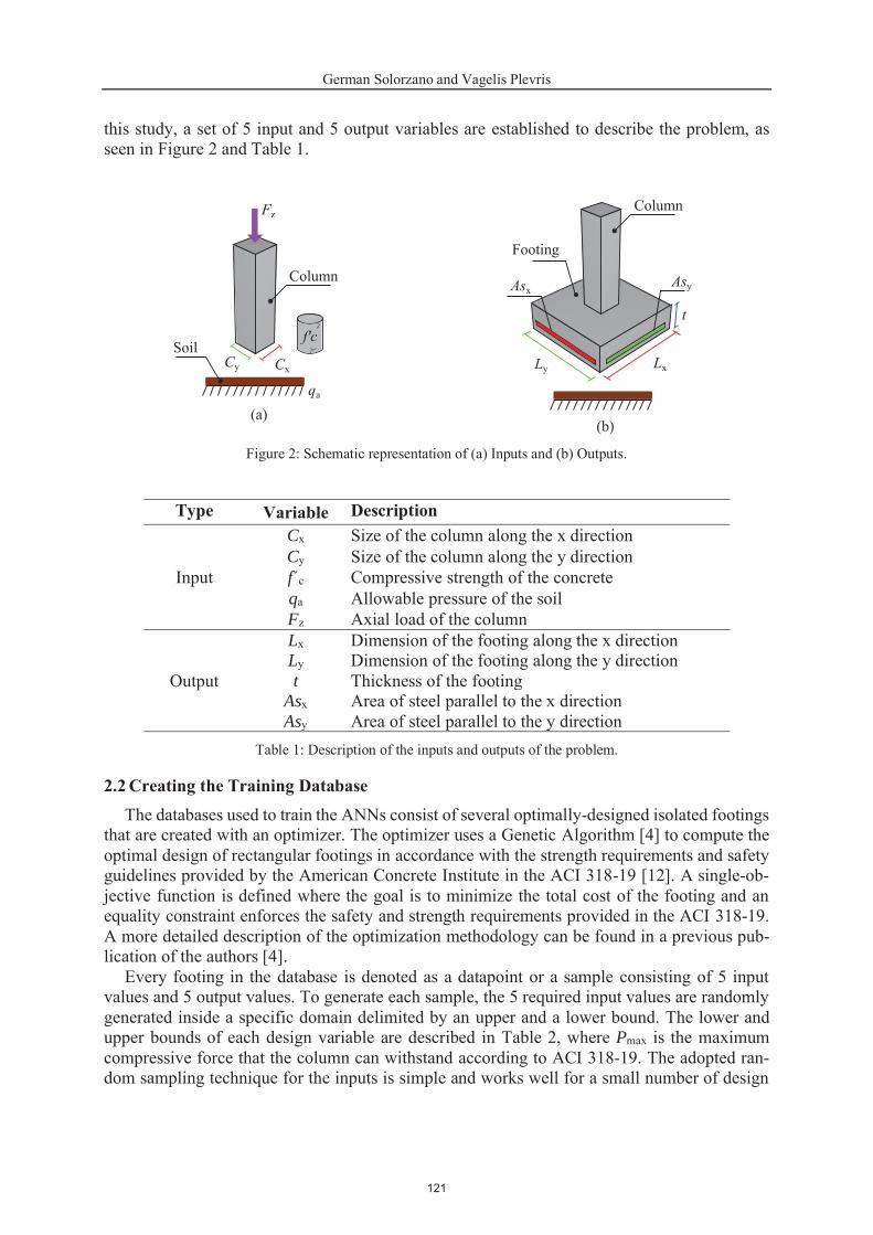
Type Variable DescriptionCCfqFLLt
AsAs
2.2 Creating the Training Database
P
121
Variable Lower Bound Upper BoundCCfqF P P
2.3 Neural Network Architecture
122
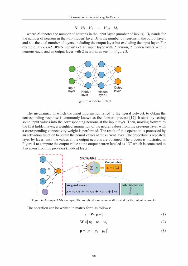
N H H … HL- MN H
i- ML
z bW p
w w wW
Tp p pp
123

O z bW p
O p; W
bσ
BPNN No of hidden layers Architecture
2.4 Training Procedure
124

n
i ii
C T pn
T p n
L L
L L L L
z pC Cw w z p
C wLzL
pLzL
wL pLpL zL
CT p
125

3 RESULTS AND DISCUSSION
3.1 Parameters Summary
3.2 Training loss
3.3 ANN performance comparison
126

127

Input Values Output Values(from GA optimizer)
C LC Lf tq AsF As
P.R.E.
128

Ground Truth
500 1000 2000 4000 8000 16,000P. R.E. P. R.E. P. R.E. P. R.E. P. R.E. P. R.E.
LL
tAsAs
Average 5.63% 4.54% 2.46% 1.14% 1.58% 0.64%
4 CONCLUSIONS
4.1 Future work
129
REFERENCES Computational Structural Engineering: Past Achievements
and Future Challenges. 4
A simple genetic algorithmfor the design of reinforced concrete beams. 13
Cost-Based Optimum Design of ReinforcedConcrete Retaining Walls Considering Different Methods of Bearing Capacity Computation. 7
Optimum Design of RC Footings with Genetic AlgorithmsAccording to ACI 318-19. 10
Optimal design forrectangular isolated footings using the real soil pressure.37
Neural networks in structural analysis and design: An overview.3
An Artificial Neural Network Model For Preliminary Design Of ReinforcedConcrete Beam Column 2002 ASEE Annual Conference
Developing a Library of Shear Walls Databaseand the Neural Network Based Predictive Meta-Model. 9
An Artificial Neural Network Approach for Prediction of BearingCapacity of Spread Foundations in Sand. 72
Prediction of Properties of FRP-ConfinedConcrete Cylinders Based on Artificial Neural Networks. 10
Modeling of Masonry Failure Surface under BiaxialCompressive Stress Using Neural Networks.55
Building Code Requirements for Structural Concrete (ACI 318-05)and Commentary
An efficient sampling scheme: Updated Latin Hypercube Sampling.7
Advances in Neural Networks in Computational Mechanics andEngineering Advances of Soft Computing in Engineering
Deep Learning
130

Back Propagation Neural Networks. 33
The perceptron: A probabilistic model for information storage andorganization in the brain. 65
On Large-Batch Training for Deep Learning: Generalization Gapand Sharp Minima 5th International Conference on Learning Representations (ICLR2017)
131

PREDICTION MODELS FOR LOAD CARRYING CAPACITY OF RC WALL THROUGH NEURAL NETWORK
Shaheera Sharib , Naveed Ahmad , Vagelis Plevris and Afaq Ahmad
Abstract
This study is focused on the development of prediction models for the determination of the loadcarrying capacity of reinforced concrete walls using Artificial Neural Networks (ANNs). A da-tabase of 95 samples is used for the RC Wall, based on available experimental studies, includ-ing various critical parameters, such as the length of web portion of the wall L , thickness ofwall boundary member b , effective depth of wall (d), height of wall H , shear span ratioa /d , vertical steel ratio ρv , horizontal steel ratio ρh , yield strength of vertical and horizon-
tal steel f , compressive strength of concrete f , and the ultimate load carrying capacityV Depending on the combination of the input parameters, 4 different ANN models are
trained by using a customized code in Matlab. Several error metrics have been used for the evaluation of the performance of the various ANN morels. The comparative study exhibited that the predictions of the ANN model are closer to the experimental values as compared to their counterpart physical models, i.e., the compressive force path (CFP) and the current designcodes, ACI and Eurocode 2.
Keywords:
132

1 INTRODUCTION
133

2 RCC SHEAR WALL DATABASE
L , thickness of wall boundary member b , (d , H ,
ρv , ρh ,f , f , V
RV
134

Description Unit Min Max Mean St.Dev COVL
bd
H ,a d ,ρ Avw bw sv
ρ Ahw bw shf
fV
R
135
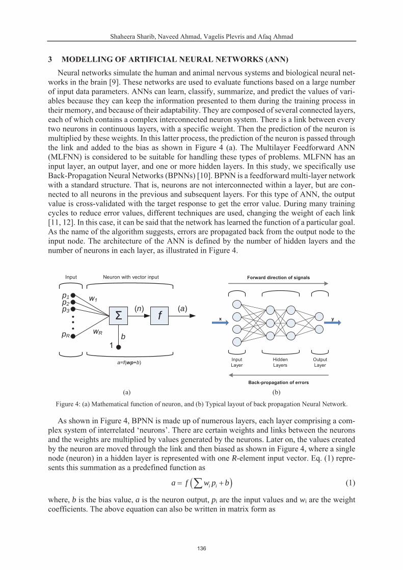
3 MODELLING OF ARTIFICIAL NEURAL NETWORKS (ANN)
R
i ia f w p b
b a p w
Σ(n)
p1
Input Neuron with vector input
a=f(wp+b)
b
f(a)
1
p2p3
pR
Input Layer
Hidden Layers
Output Layer
Forward direction of signals
x y
Back-propagation of errors
136

a f bwp
w R p R wp
i ii
E w T O
T OL ,
b , d , H ,a d , ρ , ρ ,
f , f ,V
ANN Name Set of Input Parameters used Output ParameterLw, bw, d, ,H, av/d, ρv, ρh, fy, fc
VexpLw, bw, H, av/d, fc, Mf/fcbwd2
bw/d, av/d, ρvfy/ρh, fc/fybw/d, av/d, Mf/fcbwd2, fc/fy
X XX x X xx x
x X xx x x
X X XX
X X
137

Vu Unit MIN MAX DIFF AVG SD COVV
R MSE MAEO
T R
n
i ii
n n
i ii i
T T O OR
T T O O
n
i ii
T OMSE
nn
i ii
T OMAE
n
138
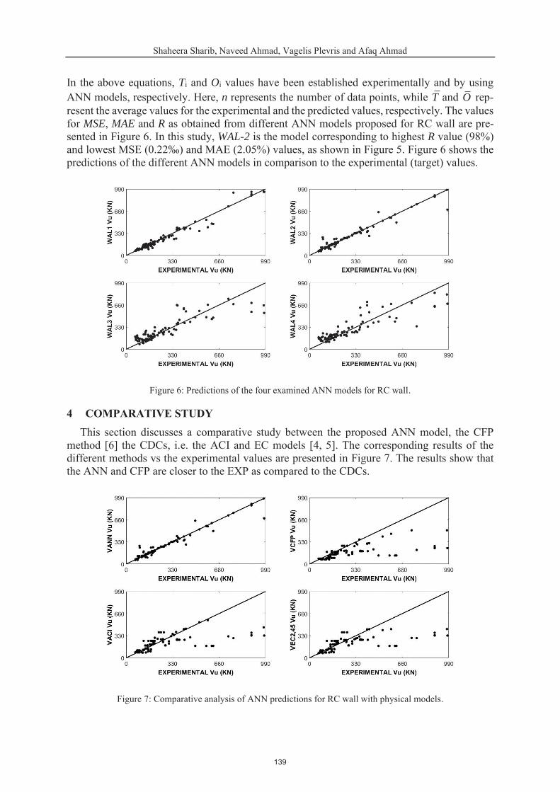
T On T O
MSE MAE RWAL-2 R
4 COMPARATIVE STUDY
139

V V
V V
V
V V
5 CONCLUSIONS
L , b ,(d), H , a d , ρ ,
140

ρ , f ,f , V
MSE MAE R
REFERENCES
Comparative study of strength of RC shear wall at different location onMulti-storied residential building.
5Seismic analysis of RCC building with and without
shear wall. 3
Behaviour and design of earthquake resistant low-rise shearwalls
Building Code Requirements for Structural Concrete (ACI 318-14) andCommentary aci-318-14
Eurocode 2: Design Of Concrete Structures - Part 1-1: General Rules And RulesFor Buildings EN 1992-1-1
Compressive Force-Path Method
Input Variable Selection in Neural NetworkModels. 43
Efficient BackpropArtificial Neural Networks: Fundamentals, Computing,
Design, And Application. 43The Backpropagation Algorithm Neural Networks
Neural Network-Based Prediction: TheCase of Reinforced Concrete Members under Simple and Complex Loading.
11Prediction of Properties of FRP-Confined
Concrete Cylinders Based on Artificial Neural Networks. 10Assessing the accuracy of RC design code predictions through the
use of artificial neural networks.10
Reliability Analysis of Strength Models for CFRP-ConfinedConcrete Cylinders.
141

Anisotropic masonry failure criterion using artificialneural networks. 28
Modeling of masonry failure surface under biaxialcompressive stress using Neural Networks. 55
Reliability analysis of proposed capacity equation forpredicting the behavior of steel-tube concrete columns confined with CFRP sheets.
25
142

PROPELLER OPTIMIZATION STRIVE TO PERFORMANCE / ACOUSTIC TRADE-OFF
Ohad Gur1, Jonathan Silver2, Radovan Dítě3, and Raam Sundhar3
1 Mechanical Design Department2 Aerodynamic Department
IAI – Israel Aerospace Industries, Lod, 70100, Israele-mail: {ogur,jsilver}@iai.co.il
3 Aerospace EngineerMejzlik Propellers s.r.o., Brno-Židenice, 61500, The Czech Republic
e-mail: {dite,sundhar}@mejzlik.eu
Abstract
This paper describes the design of a propeller-based electric-propulsion system for hover condition. The design procedure harnesses modeFRONTIER optimization framework with various single- and multi-objective hybrid optimization schemes. Several analyses were inte-grated to the design framework and propeller geometry optimizations were conducted.The multi-objective problem consisted of trade-off between the contradicting goals of perfor-mance (required electric power at hover) and acoustics (tonal overall sound-pressure-level). Using various hybrid optimization schemes, the Pareto tradeoff fronts were found for 2, 3, and 4 bladed propellers. These propellers are compared to an off-the-shelf propeller blade (Mejzlik 18x6) which is used as a reference. This reference propeller proves to be good de-sign, compared to the optimized results. Still, from the optimized Pareto results, 4 propeller configurations were chosen to be fabricated and tested. These configurations are optimized by their acoustic or performance trade-off. These optimized propellers represent a good com-promise, which is better than the reference propeller.
Keywords: Propeller, Performance, Acoustic, Electric, UAM, Optimization, MDO
143
EUROGEN 2021 14th ECCOMAS Thematic Conference on
Evolutionary and Deterministic Methods for Design, Optimization and Control N. Gauger, K. Giannakoglou, M. Papadrakakis, J. Periaux (eds.)
Streamed from Athens, Greece, – 2021
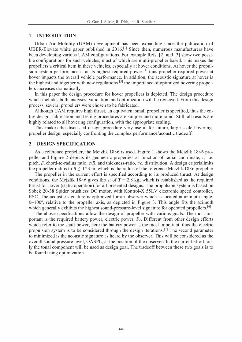
O. Gur, J. Silver, R. Dítě, and R. Sundhar
1 INTRODUCTIONUrban Air Mobility (UAM) development has been expanding since the publication of
UBER-Elevate white paper published in 2016.[1] Since then, numerous manufacturers have been developing various UAM configurations. For example Refs. [2] and [3] show two possi-ble configurations for such vehicles; most of which are multi-propeller based. This makes the propellers a critical item in these vehicles, especially at hover conditions. At hover the propul-sion system performance is at its highest required power,[4] thus propeller required-power at hover impacts the overall vehicle performance. In addition, the acoustic signature at hover is the highest and together with new regulations [5] the importance of optimized hovering propel-lers increases dramatically.
In this paper the design procedure for hover propellers is depicted. The design procedure which includes both analyses, validation, and optimization will be reviewed. From this design process, several propellers were chosen to be fabricated.
Although UAM requires high thrust, an equivalent small propeller is specified, thus the en-tire design, fabrication and testing procedures are simpler and more rapid. Still, all results are highly related to all hovering configuration, with the appropriate scaling.
This makes the discussed design procedure very useful for future, large scale hovering-propeller design, especially confronting the complex performance/acoustic tradeoff.
2 DESIGN SPECIFICATIONAs a reference propeller, the Mejzlik 18×6 is used. Figure 1 shows the Mejzlik 18×6 pro-
peller and Figure 2 depicts its geometric properties as function of radial coordinate, r, i.e. pitch, β, chord-to-radius ratio, c/R, and thickness-ratio, t/c, distribution. A design criterialimits the propeller radius to R ≤ 0.23 m, which is the radius of the reference Mejzlik 18×6 propeller.
The propeller in the current effort is specified according to its produced thrust. At design conditions, the Mejzlik 18×6 gives thrust of T = 2.8 kgf which is established as the required thrust for hover (static operation) for all presented designs. The propulsion system is based on Sobek 20-38 Spider brushless DC motor, with Kontrol-X 55LV electronic speed controller, ESC. The acoustic signature is optimized for an observer which is located at azimuth angle,θ=100º, relative to the propeller axis, as depicted in Figure 3. This angle fits the azimuth which generally exhibits the highest sound-pressure-level signature for operated propellers.[6]
The above specifications allow the design of propeller with various goals. The most im-portant is the required battery power, electric power, Pe. Different from other design effortswhich refer to the shaft power, here the battery power is the most important, thus the electric propulsion system is to be considered through the design iterations.[7] The second parameter to minimized is the acoustic signature as heard by the observer. This will be considered as the overall sound pressure level, OASPL, at the position of the observer. In the current effort, on-ly the tonal component will be used as design goal. The tradeoff between these two goals is to be found using optimization.
144
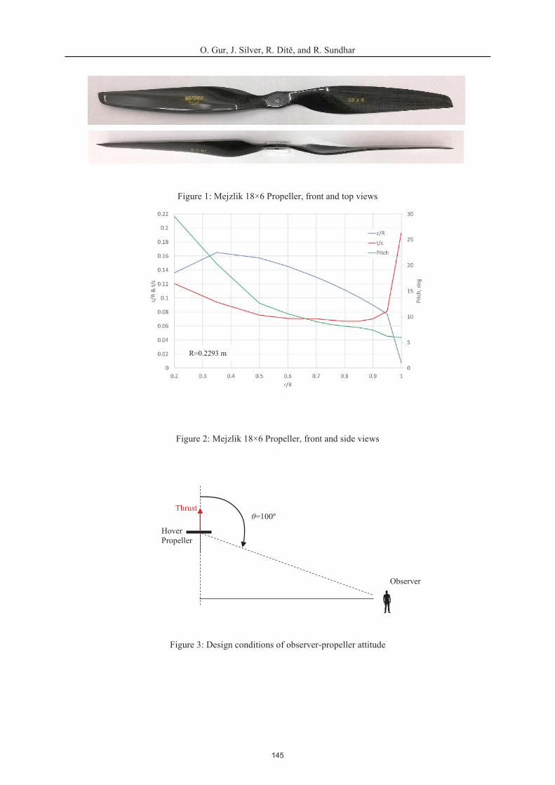
O. Gur, J. Silver, R. Dítě, and R. Sundhar
Figure 1: Mejzlik 18×6 Propeller, front and top views
Figure 2: Mejzlik 18×6 Propeller, front and side views
Figure 3: Design conditions of observer-propeller attitude
R=0.2293 m
θ=100ºThrust
Hover Propeller
Observer
145

O. Gur, J. Silver, R. Dítě, and R. Sundhar
3 PROPELLER’S ANALYSESTo allow proper optimization, the required analyses should be both accurate and efficient,
i.e. using low computer resources. In this case, three analyses are used: propeller performance, electric system, and propeller acoustic analysis.
3.1 Propeller Performance AnalysisThe propeller performance model is based on blade-element model (BEM) which was ex-
tensively validated in the past.[8] Although, most past validation cases were of axial flight re-gime, in the current case hover condition is treated which was also validated.[7]
BEM analysis uses a 2-D aerodynamic database based on the geometry of the propeller cross sectional airfoils. Accuracy of the 2-D aerodynamic database is an important part of BEM level-of-confidence. Thus, substantiation of the current database was conducted using EZair RANS (Reynolds Average Navier-Stokes) software.[9] In addition, some installation losses, due to the propeller and test rig interaction, were implemented on the BEM analysis.
3.2 Electric System AnalysisIn the current effort a simple motor model is used to find the required electric power. The
model is based on four parameters: speed constant, Kv, armature resistance, Ra, no-load cur-rent, I0, and controller efficiency, ηc.[10] The model is based on the following assumptions:
a. Power factor is equal to unit. This assumption is applicable to small brushless Perma-nent Magnet (PM) motors.
b. Magnetic losses (eddy/Foucault Current and magnetic hysteresis) can be neglected.
3.3 Acoustic AnalysisThe current acoustic model predicts only the tonal noise of the propeller. The model is
based upon Farassat’s formulation[11] as used in former design cases[12]. The model went through extensive validation for various cases of propeller on various flight regimes.[13],[14]
4 OPTIMIZATIONDesign technique is similar to former cases accomplished with the same tools. These tools
include using the validated analysis tools (BEM, electric model, and acoustic model) together with Esteco’s modeFRONTIER framework.[13],[7]
Figure 4 presents a screen capture of modeFRONTIER framework. This design environ-ment enables the integration of different simulation models into a single synergetic design tool. In addition, it allows the use of various optimization procedures, thus a multi-disciplinary design optimization, MDO, tool is obtained. In the current case, first the propeller performance is calculated and then the propeller acoustic is estimated. The use of mode-FRONTIER enables an easy usage of any of the input or output parameters, either as design variables or to include it in the goal function and constraints.
In addition, a geometric pre-analysis and performance post-analysis, are implemented us-ing Excel spread sheet. The geometry pre-analysis is used to parametrize the design variables which are the pitch, β, thickness-ratio, t/c, and chord-to-radius ratio, c/R, distribution along the blade. The current effort uses a Bezier spline to achieve smooth distribution of the geome-try, hence 6 design parameters are used for each distribution. Thus, the design problem con-tains total of 18 design variables. All airfoils are based on the Mejzlik 18×6 cross sections,and the propeller radius is fixed to R=0.23 m.
146

O. Gur, J. Silver, R. Dítě, and R. Sundhar
To ensure the structural properties of the optimized designs, two geometric constraints are satisfied. First the blade thickness distribution should not be lower than the original Mejzlik 18×6. Thin blade might be “soft” or exposed to high stresses, which might cause unacceptable aeroelastic behavior, and high deflections. In addition, the root chord should not be larger than the Mejzlik 18×6’s root chord. This might cause a very thick hub which increases the propel-ler weight.
To overcome these issues, the design procedure incorporated two geometric constraints over the thickness distribution and root chord. The first constraint limits the thickness distri-bution and the second the rood chord. The thickness distribution, t (not t/c) has to be higher or equal to the Mejzlik 18×6 up to r/R=0.90, with a tolerance of 0.1 mm. The blade tip (0.9< r/R <1) was freed from this constraint – the impact over the design was high and it seems the im-portance of this constraint, at the very tip of the blade, is less important. The root chord is lim-ited to c/R < 0.15. Note that the Mejzlik 18×6’s c/R = 0.14 at the root (Figure 2), thus small increase of the root chord is allowed.
The performance post-analysis excel module is used to find the propeller-motor matching speed. Using the performance calculation, for given propeller geometry, several rotational speeds are calculated. To find the correct rotational speed, which the propeller produces the required thrust, T =2.8 kgf, a linear interpolation is used. Then, using the electric model the electric power, Pe, is found.
Figure 4: modeFRONTIER design framework screen capture
Performance Calculation
AcousticCalculation
Electric system / Propeller Matching
Geometric pre-analysis
147

O. Gur, J. Silver, R. Dítě, and R. Sundhar
Separate optimizations procedures were conducted for 2,3, and 4 bladed propellers. The aim is to find, for different number-of-blades, the tradeoff between the electric power and the overall sound-pressure-level, OASPL, as defined in the problem specification of section 2.
For each specific number-of-blades, the first stage is to find the Utopia Point in the design-goal space. For a multi-objective problem containing two different cost-functions, this is ac-complished by two separate single-objective optimizations; the first using the electric power as an objective and the second using the OASPL as the design goal objective. To demonstrate the procedure, the 2-bladed case is considered in what follows.
The single-objective optimizations are conducted using hybrid-optimization scheme based on the available methods in modeFRONTIER. This hybrid scheme can be easily transfer to any other available optimization framework.
First, pilOPT scheme is used. This is highly autonomous method which uses multi-strategy self-adapting algorithm. No design-of-experiment, DOE, is required, nor any other a-prioridefinition. pilOPT harnesses both surrogate-based (response surface) methods and implicit-optimization methods, thus combines both local and global search techniques.
Using pilOPT, some candidates for further optimization are chosen. These are used as ini-tial guess for constrained gradient-based optimization. In the current effort, sequential quad-ratic programming, SQP, is used. Each initial guess is optimized into better design; thus apopulation of optimized solutions are gathered. These are finally used as the initial population for genetic algorithm, GA, scheme, which hopefully finds the global-optimal solution.
Figure 5 shows the results for the two single-objective procedures, conducted for the 2-bladed case. The left column is the minimum electric power, Pe, while the left column is the minim overall sound-pressure-level OASPL. The upper charts show the progress of the cost-function as function of the iteration, Lower charts includes the same results in cost-function space.
Each analysis lasts about 5 sec. on a desktop computer using 8 parallel threads of calcula-tion. The entire optimization scheme last about 5÷10 hours, mostly over-night. Some differ-ences between the two cases are visible, mostly for the ratio between the SQP and GA analysis. While the min. Pe case uses much more iteration of SQP, the min. OASPL uses more iterations of GA scheme.
In addition, for the min Pe, the SQP procedure went into a local minimum. Then, the GAscheme “escaped” from this minimum into better region, supposedly global minimum. This is very common for gradient based methods such as SQP to converged to a local minimum. GA is less accurate with its minimum location, but it is capable of hopping to various minimum regions, i.e. global search capabilities. In comparison to the minimum Pe, the minimumOASPL case exhibits the ability of SQP to locate an optimum which later was improved by the GA scheme. This Hybrid usage of various different scheme, harnesses each scheme’sstrength to a synergetic optimization procedure.
Note that the designer should carefully monitor the optimization and decide when to move from one method to the other, and which DOE to re-use when transferring from pilOPT to SQP and then from SQP to GA.
Gathering both results of the two single-goal optimization is presented in Figure 6. On this figure also the reference Mejzlik 18x6 propeller is presented as a green circle. The cloud of results can be used to substantiate DOE which is then used to optimize the Pareto frontier. This is done using a multi-goal scheme, in the current case mainly by MOGA and NSGA schemes. The final Pareto frontier after optimization is presented as a black curve in Figure 6.Note that the cloud of results from the two single-objective optimizations, draw the final Pare-to with relatively good accuracy. Thus, the Utopia-point estimation, actually plays an im-portant role for the multi-objective scheme.
148

O. Gur, J. Silver, R. Dítě, and R. Sundhar
Figure 5: 2-blades Utopia Point, single-objective optimization resultsLeft: minimum electric power, Pe, Right: minimum overall sound-pressure-level OASPL
Figure 6: 2-blades single-objective results compared to the reference Mejzlik 18x6 and final Pareto frontier
Min. Pe
Min. Pe
Min. OASPL
Min. OASPL
149

O. Gur, J. Silver, R. Dítě, and R. Sundhar
The multi-goal optimization was conducted 3 times for 2, 3, and 4 blades configurations. Each uses the same procedure mentioned above. Pareto frontiers which resulted from the op-timization are presented in fig. 7. Propellers based on the Mejzlik 18×6 blades are also marked by red circles. The design influence of number-of-blades is prominent – increased number-of-blades causes both OASPL decrease and Pe increase – a tradeoff which the de-signer should consider carefully.
From these Pareto frontiers, 4 propeller configurations were chosen – these are marked with arrows in fig. 7 and include:
a. 2 blades, minimum Pe (2B min Pe)b. 2 blades, minimum SPL (2B min SPL)c. 3 blades, minimum Pe (3B min Pe)d. 4 blades, minimum Pe (4B min Pe)These selections are based on motivation for improving the already adequate Mejzlik 18x6,
on different aspects. The minimum Pe is being chosen as improved Pe without penalizing the OASPL. Similarly, min. OASPL is chosen with no penalty over Pe.
The propeller characteristics are depicted in table 1, and their blade geometric parameters in fig.8. The clear difference is the rotational speed. This appears both as the mechanism of reducing the OASPL for the 2 blades propeller and for achieving the proper thrust for the 3 and 4 bladed propeller. To reduce the rotational speed, thus achieving min SPL for the 2 blad-ed propeller, the pitch was increased and the chord slightly increased as well.
For the 3 and 4 blades, the rotational speed had to decrease to achieve the required thrust,T=2.8 kgf. The chord cannot decrease due to the geometric constraint, thus the chord re-mained similar and thickness remains above the Mejzlik 18×6 blade. To maintain high enough rotational speed, the pitch decreases for the 3 and 4 bladed propellers, thus the electric efficiency, ηe, and figure-of-merit, FM, remain relatively high.
While the 3-bladed propeller exhibits high FM and low ηe, the 4-bladed exhibits low FM and high ηe. Generally, all tradeoff in such complex design case, is beyond simple intuition and it is a result of handling with all constraints while striving to minimize all design goals. This proves the advantage of such MDO (multidisciplinary design optimization) framework, which takes contradicting requirements and find the best compromise.
150

O. Gur, J. Silver, R. Dítě, and R. Sundhar
2B min Pe
2B min SPL
3B min Pe
4B min Pe
Figure 7: Pareto frontiers for the optimized resultsRed circles mark the results for propeller based on Mejzlik 18×6 blades
2-Blades Mejzlik 18×6
2-Bladesmin.Pe
2-Bladesmin.SPL
3-Bladesmin.Pe
4-Bladesmin.Pe
Electric Power, Pe, W 445 425 445 455 495Shaft Power, Pshaft, W 340 335 345 350 375Engine Speed, Ω, rpm 5,100 5,200 4,600 4,700 4,500Figure-of-merit, FM 0.68 0.69 0.67 0.66 0.62Electric efficiency, ηe 0.77 0.79 0.77 0.67 0.76Tonal OASPL, dB 66.1 66.1 64.7 56.9 48.3
Table 1: Optimized propeller characteristics
151

O. Gur, J. Silver, R. Dítě, and R. Sundhar
Figure 8: Optimized blade geometries
152

O. Gur, J. Silver, R. Dítě, and R. Sundhar
5 CONCLUSIONSIn this paper a comprehensive and methodic design process for hover-propeller is de-
scribed. The design process has to have a detailed specification which is based, in the current case, on an existing propulsion system with of-the-shelf propeller. In the basis of the design process are 3 analytic models: blade-element model for the propeller performance estimation, electric model for the propulsion system characteristics, and acoustic model which analyzesthe propeller tonal sound-pressure-level. Each of these models was previously validated ver-sus various results in the literature.
These analyses were incorporated in a design framework based on modeFRONTIER soft-ware and a multidisciplinary-design-optimization environment was substantiated. This envi-ronment includes, beside the analyses, various definitions of design variables, constraints, and design goals. Hence a multi-objective optimization problem is defined.
The design framework was run 3 times for designing 2, 3, and 4 bladed propellers. First, aUtopia-point was found using a single-goal optimization process, which resulted with mature design-of-experiment for the final multi-goal scheme. The optimization harnesses various schemes such as multi-strategy, gradient-based, and evolutionary.
The optimization scheme was resulted with a Pareto frontier which exhibits the tradeoff between the propulsion-system performance and its acoustic signature. From these tradeoffs, optimized propeller configurations were chosen. These are to be fabricated and tested. The test results for both performance and acoustics is to be compared with the design trends, thus the design process is to be validated.
In the current effort 4 propeller were resulted. Two of them are 2 bladed, minimal electric power and minimal acoustic signature. In addition, 3 bladed and 4 bladed propellers for min-imum electric power were chosen. The four propellers exhibited some improvements over the reference of-the-shelf propeller. These improvements can be chosen by the designer according to the resulted Pareto frontiers. This demonstrates the use of Pareto tradeoff results as a quan-titative, important decision support tool, during design process.
ACKNOWLEDGMENTSThe research was funded by Israel-Europe Research & Innovation Directorate, ISERD, of
the Israel Innovation Authority, and DELTA-2 programme of the Technology Agency of the Czech Republic, TAČR. The authors thank these two organizations for their generous contri-butions.
153

O. Gur, J. Silver, R. Dítě, and R. Sundhar
REFERENCES [1] UBER Elevate, “Fast-Forwarding to a Future of On-Demand Urban Air Transporta-
tion,” October 2016 [URL: https://www.uber.com/il/he/elevate/ Cited: September 2020]
[2] S. Rogers, “This Passenger Drone Is Set to Have Its First Test Flight Next Week,” Jan-uary 2018 [URL: https://interestingengineering.com/this-passenger-drone-is-set-to-have-its-first-test-flight-next-week Cited: September 2020]
[3] A. Douglas, “Honeywell and Volocopter sign navigation solutions R&D deal,” Com-mercial Drone Professional April 2019 [URL: https://www.commercialdroneprofessional.com/honeywell-and-volocopter-sign-navigation-solutions-rd-deal/ Cited: September 2020]
[4] Gur O, Lazar G., and Yaniv A., "Electric VTOL UAV prop-rotor MDO," 52nd Israel Annual Conference on Aerospace Sciences, February 29 – March 1st, 2012, Israel
[5] EASA, “COMMISSION DELEGATED REGULATION (EU) 2019/945, of 12 March 2019 on unmanned aircraft systems and on third-country operators of unmanned aircraft systems,” Official Journal of the European Union, March 2019 [URL: https://eur-lex.europa.eu/legal-content/EN/TXT/PDF/?uri=CELEX:32019R0945&from=EN Cited: September 2020]
[6] The Royal Aeronautical Society, “Estimation of the maximum discrete frequency noise from isolated rotors and propellers,” ESDU 76020, February 2018
[7] Gur O, Lazar G., "Prop-rotor design for an electric tilt-rotor vehicle," American Heli-copter Society, Future Vertical Lift Aircraft Design Conference, January 18-20, 2012, Fisherman’s Wharf, San Francisco, California
[8] Gur O. and Rosen A., “Comparison between blade-element models of propellers”, 48th Israel Annual Conference on Aerospace Sciences, February 27-28, 2008, Israel.
[9] Y. Kidron, Y. Levy, and M. Wasserman, “The EZAir CFD Solvers Suite: EZAir Theo-retical and User’s Manual - Version 3.54,” Tech. Rep. August, ISCFDC, 2016.
[10] Gur O. and Rosen A., “Optimization of electric UAV propulsion system,” Journal of Aircraft, Vol. 46, No. 4, July-August 2009, pp. 1340-1353
[11] Farassat, F., and Succi, G. P., “A Review of Propeller Discrete Frequency Noise Predic-tion Technology with Emphasis on Two Current Methods for Time Domain Calcula-tions,” Journal f Sound and Vibration, Vol. 71, No. 3, 1980, pp. 399–419
[12] Gur O. and Rosen A., “Design of quiet propeller for an electric mini unmanned air vehi-cle,” Journal of Power and Propulsion, Vol. 25, No. 3, May-June 2009, pp.717-728
[13] Gur O. and Rosen A., “Optimization of Propeller Based Propulsion System,” AIAA Journal of Aircraft, Vol. 46, No. 1, January-February 2009, pp. 95-106
[14] Gur O., “Toward Optimal Design of Contra-Rotating Propulsion System - Practical Acoustic Analysis,” 1st Aerospace Europe Conference AEC2020 Bordeaux, France, 25–28 February 2020
154

EFFICIENT AND ACCURATE MODELING OF NON-PRISMATIC BEAMLIKE STRUCTURES
G. Migliaccio1
1 Civil and Industrial Engineering, University of Pisa, National Group of Mathematical Physics, Pisa
Largo Lucio Lazzarino 2, 56122, Pisa, Italy e-mail: [email protected]
Abstract
Many complex engineering structures, e.g. components of helicopters, wind turbines, aircraft wings and propellers, are beamlike and non-prismatic. Structures of this kind may be tapered, pre-twisted, and even curved in their unstressed state, and undergo large displacements and 3D cross-sectional warping. Their mechanical modeling can be addressed via non-prismatic beam elements providing the appropriate compromise between computational efficiency and accuracy. Over the years many models have been proposed for beamlike structures, but gen-eral non-prismatic cases still require investigation. Formulas valid for prismatic beams, for example, generally provide incorrect results in non-prismatic cases, as the variation in the dimensions and orientation of the transverse cross-sections produce non-trivial stress distri-butions absent in prismatic beams. A model suitable for the aforementioned non-prismatic elements should properly describe their shape, explicitly consider the effects of their geomet-ric design features on their stress and strain fields, account for large displacements, and pro-vide the known results of prismatic cases. We propose a physical-mathematical model that accounts for all such requirements. The non-prismatic beam is seen as a collection of plane figures (the transverse cross-sections) attached at a 3D curve (the beam’s centre-line). The centre-line’s points may undergo large displacements. The transverse cross-sections are fully deformable and may undergo warpings in and out of plane. Assuming small warping and strain fields, a variational approach provides the field equations. The model obtained enables evaluating even analytically the effects of geometric parameters (such as taper) on the stress and strain fields. Numerical examples and comparisons with the results of nonlinear 3D-FEM analyses confirm the effectiveness of the proposed modeling approach.
Keywords: Non-prismatic beams, tapered cross-sections, large displacements.
155
EUROGEN 2021 14th ECCOMAS Thematic Conference on
Evolutionary and Deterministic Methods for Design, Optimization and Control N. Gauger, K. Giannakoglou, M. Papadrakakis, J. Periaux (eds.)
Streamed from Athens, Greece, – 2021

G. Migliaccio
1 INTRODUCTION Ongoing efforts to predict the mechanical behavior of non-prismatic beamlike structures,
by using increasingly accurate and computationally efficient models, are aimed at optimizing their performance and cost. At the same time, tackling complex engineering problems contin-uously leads to develop theories to meet ever more stringent requirements on the predictive models. For example, several theories have been developed over the years for helicopter blades with pre-twist, a geometric feature which induces several couplings in their mechanical response: for pre-twisted beams bending is always three-dimensional, and tension may be significantly coupled to torsion [1-6]. Wind turbine blades are another interesting example of pre-twisted structures. Moreover, they are also characterized by important spanwise variations in the dimensions of their transverse cross-sections, that is, they are also tapered [7-8]. Their shape alone makes predicting their mechanical behavior a very challenging task. Not to speak of the large displacements they may undergo, which further complicate the study and deriva-tion of analytical closed-form formulas for engineering design purposes.
Generally speaking, structural analyses show that the models and formulas commonly used for prismatic beams provide incorrect results in non-prismatic cases, as the variations in the dimensions and orientation of the transverse cross-sections produce non-trivial stress distribu-tions absent in prismatic beams [9-10]. To date several models have been proposed for beam-like bodies, ranging from linear theories [11-13] to geometrically exact and asymptotic approaches [14-20]. However, investigations are still required to develop rigorous yet applica-tion-oriented models for three-dimensional non-prismatic beams, which explicitly account for important geometric features (such as taper), account for large displacements, directly furnish the 3D stress and strain fields, and provide known results in prismatic cases.
This paper presents a physical-mathematical model that meets all such requirements for non-prismatic beams having fully deformable cross-sections and undergoing large displace-ments and small strains. The general model is introduced in section 2. Analytical results for bi-tapered and pre-twisted beams are presented in section 3. Numerical examples and compar-isons with the results of nonlinear 3D-FEM analyses are finally shown in section 4.
2 MECHANICAL MODEL In this section we introduce the main ingredients of our model, further details of which can
be found in [21]. Then, we present tapered beams for which we can provide analytical formu-las for evaluating their stress and strain fields (section 3) and, subsequently, provide compari-sons with the results of nonlinear 3D-FEM simulations (section 4).
2.1 Geometry and strain measures The beam is seen as a collection of plane figures (transverse cross-sections) attached at a
3D curve (beam’s centre-line). The cross-sections are fully deformable and may undergo dis-placements in and out of plane (all called warping displacements). The displacement of each cross-sectional point from the reference to the current state consists of a rigid part (similarly to the beam theories with rigid cross-sections) onto which the aforementioned warping motion is superposed. Figure 1 shows a schematic of the beam’s reference and current states.
Two local triads of orthogonal unit vectors are introduced in Figure 1. The first, bi, in the reference state, with b1 tangent to the centre-line, depends on the reference arc-length s, i.e. bi=bi(s). The second, ai, is an image of bi in the current state and depends on the arc-length s and time t, i.e. ai=ai(s,t). A third triad, ci, pertains to a fixed Cartesian reference frame.
156
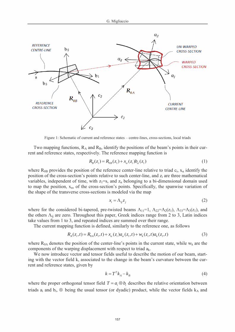
G. Migliaccio
Figure 1: Schematic of current and reference states – centre-lines, cross-sections, local triads
Two mapping functions, RA and RB, identify the positions of the beam’s points in their cur-rent and reference states, respectively. The reference mapping function is
0 1 1( ) ( ) ( ) ( )B i B iR z R z x z b z (1)
where R0B provides the position of the reference center-line relative to triad ci, xα identify the position of the cross-section’s points relative to such center-line, and zi are three mathematical variables, independent of time, with z1=s, and zα belonging to a bi-dimensional domain used to map the position, xα, of the cross-section’s points. Specifically, the spanwise variation of the shape of the transverse cross-sections is modeled via the map
i ij jx z (2)
where for the considered bi-tapered, pre-twisted beams Λ11=1, Λ22=Λ2(z1), Λ33=Λ3(z1), and the others Λij are zero. Throughout this paper, Greek indices range from 2 to 3, Latin indices take values from 1 to 3, and repeated indices are summed over their range.
The current mapping function is defined, similarly to the reference one, as follows
0 1 1 1( , ) ( , ) ( ) ( , ) ( , ) ( , )A i A i k i kR z t R z t x z a z t w z t a z t (3)
where R0A denotes the position of the center-line’s points in the current state, while wk are the components of the warping displacement with respect to triad ak.
We now introduce vector and tensor fields useful to describe the motion of our beam, start-ing with the vector field k, associated to the change in the beam’s curvature between the cur-rent and reference states, given by
TA Bk T k k (4)
where the proper orthogonal tensor field i iT a b describes the relative orientation between triads ai and bi, being the usual tensor (or dyadic) product, while the vector fields kA and
157

G. Migliaccio
kB are such that i A ia k a and i B ib k b , ˄ being the usual cross-product and apex-prime denoting the derivative with respect to s (further details are in [21]).
Along with k, we introduce another vector field, γ, which is related to the difference be-tween the center-line tangent vectors of the current and reference states, as follows
0 0T
A BT R R (5)
Note that γ and k, which vanish for rigid motions and are invariant under superposed rigid motion [20], are referred to here as 1D strain measures. The Green-Lagrange strain tensor E is instead referred to here as 3D strain measure and is written in a form based on the assumption of small strain and warping fields considered in this work. In particular, we assume that the characteristic dimension of the transverse cross-sections, h, is much smaller than the reference length, L, of the centre-line (i.e. the beam is slender); the beam’s curvatures are much smaller than 1/h; the warping fields, wk, are considered small in the sense that their maximum order of magnitude is hε (ε<<1 being a non-dimensional parameter), while the order of their derivative with respect to z1 is at most εh/L. In general, all components of the strain measures are con-sidered small in the sense their order of magnitude is at most ε. For the considered beam, the strain tensor E is written (as in [9]) in the form
2
T TT H H TE I2
T H HTT H H (6)
where H is the gradient of transformation between the reference and current states
A
B
RHR
(7)
2.2 Stress measures and balance equations The stress fields in our beam are determined supposing it to be elastic. For small strains the
second Piola-Kirchhoff stress tensor S is linearly related to the strain tensor E, as follows
S EE (8)
where is the classical elasticity tensor [22], which characterizes the beam’s material behav-ior (e.g. isotropic or not). For completeness’ sake, we also introduce the first Piola-Kirchhoff stress tensor P and Cauchy stress tensor C, which for our beam are P=TS and C=TSTT (as in[9]). By using the stress tensor P, cross-sectional stress resultants are defined in terms of two vector fields, F (force) and M (moment), as follows
1
1
i i
i i
F P a
M x P a a(9)
where Σ is the cross-sectional domain and ij i jP P a b .We now exploit the principle of expended power to derive balance equations for our beam-
like body, which is three-dimensional and hyper-elastic [22]. To this end, its interactions with the external environment are quantified, for each velocity field attainable by the body, via the following functional, Πe, called the external power
e V Vp v b v (10)
158

G. Migliaccio
In (10), b are body loads per unit body’s reference volume V, p are surface tractions per unit area of the reference boundary ∂V, and v is the referential description of the time rate of the current position of the body’s points, given by
0v v x a ww (11)
where w• is the time rate of the warping displacement. Interactions among different parts of the body are instead quantified via the functional Πi, called the internal power
i V
ddt
(12)
where Φ (body’s energy density) is half the scalar product of tensors S and E, i.e. 2Φ=S∙E.According to the principle of expended power, for any velocity field attainable by the body,
its interactions with the external environment and among its parts are such that at any value of the evolution parameter t the total power vanishes (i.e. Πe=Πi). The exploitation of such prin-ciple is a usual technique in continuum mechanics to obtain balance equations in terms of the problem’s unknowns (see, e.g., [20-22]). In our case, it enables writing balance equations for the stress resultants, F and M, in the form
0 0A
F + f = 0M R F m
(13)
where f and m are the resultants of the body and contact actions per unit length of reference centre-line. The same principle also enables writing balance equations to determine the warp-ing fields wk. In particular, in the case the body loads and surface tractions on the beam’s lat-eral surface are neglected in calculating the warping fields, or vanish, it is possible to reduce the determination of the warping fields to those that verify the variational condition
0V
(14)
where δ denotes the variation of the energy function with respect to the warping fields. Note that warping fields satisfying condition (14) can be obtained numerically or, in particular cas-es, analytically, as solutions of the corresponding Euler-Lagrange equations [23].
So far we have introduced the main ingredients of our modeling approach. Specifically, we have sketched the body’s shape, which is three-dimensional and beamlike, and have defined the strain measures, stress measures, and balance equations we use to describe its mechanical behavior. By using such ingredients, the resolution of the three-dimensional nonlinear elas-ticity problem is now reduced to the solution of two main problems: the first governs the cross-sectional warping motion and it’s strong formulation can be given in terms of partial differential equations (PDEs) defined over a reference bi-dimensional domain (as is discussed in the next section). The second problem governs the centre-line motion and can be expressed in terms of a set of non-linear ordinary differential equations (ODEs) defined over a reference line (as in [9], for instance). It is worth noting that this approach reduces the computational effort and produces accurate results compared to nonlinear 3D-FEM approaches (as is shownalso in the following). Moreover, the results obtained with our model enable evaluating even analytically the effects of important geometric features, such as the cross-sectional taper, on the stress and strain fields in all points of the considered beamlike bodies. The analytical re-sults obtained in this work are presented in the next section 3 and, subsequently, are compared to the results of nonlinear 3D-FEM approaches (section 4).
159

G. Migliaccio
3 ANALITYCAL RESULTS In order to determine the stress and strain fields in our beam we need to exploit the varia-
tional condition (14). In particular, considering the corresponding Euler-Lagrange equations, in which we keep the terms up to the order εh/L, we can obtain a set of partial differential equations (PDEs) with Neumann-type boundary conditions the solution of which enables de-termining the components of tensor E. In doing this, hereafter we choose the current local tri-ads to be tangent to the center-line and focus on the case of bi-tapered beams the material properties of which are described in terms of just two material constants (i.e., Young’s modu-lus Y, and Poisson’s ratio υ). The effects of other geometric features (e.g. centre-line curva-ture), as well as those related to the material non-homogeneity and anisotropy, will be addressed in subsequent works.
Proceeding as in [21], the components E11, E21, and E31 of E, related to the out-of-plane de-formation of the transverse cross-sections, can be written in the form
11 2 3 3 2 1 1,1 1 3 1,2 2 1,3
121 1,2 1 3 2 2 3 3 2 1 2 2 2 1 3
131 1,3 1 2 3 2 3 3 2 1 3 3 3 1 2
( )
2 2(1 )( )( )
2 2(1 )( )( )
B
B
B
E k x k x e k x e x e
E e k x e k x k x x k x
E e k x e k x k x x k x
(15)
where ij i jE E b b , subscript-comma denotes the derivative with respect to xi, and the sca-lar fields e1, e2, e3 are solutions of the following PDEs problems
1,22 1,33
1,2 1 3 2 1,3 1 2 3
2,2 3,3 2 2 3 3
3,2 2,3 2 2 3 3 1
2 2 3 3
0
( ) ( ) 0
0
e e in
e k x n e k x n on
e e d x d x ine e g x g x g ine n e n on
(16)
In (16), Σ and ∂Σ are the cross-sectional domain and its boundary, nα are the components of the outward unit normal vectors on ∂Σ, and coefficients dα and gk are given by
1 12 3 3 3 2 2 3
1 13 2 2 2 3 3 2
1 1 11
2 2 2 2 2 1 31
3 3 3 3 3 1 2
2(1 ) 2(1 ) 2
2(1 ) 2(1 ) 2
2 (2 2 )2 2(1 ) 2 (3 2 )
2 2(1 ) 2 (3 2 )
B
B
B
d k k
d k k
g kg k k k k
g k k k k
(17)
It is worth noting that the PDEs equations (16) formally resemble those for flexure and tor-sion of a Saint-Venant’s cylinder. Unfortunately, PDEs problems of this kind can be solved in closed-form only for a few cases, but this is not surprising (this happens even in the linear theory of prismatic beams [11-13]). However, they can always be solved with the aid of nu-merical methods for all other cases as well. Regarding our PDEs problem (16)-(17), we more-over note that its solution can generally be expressed as linear combinations of the 1D strain measures, γ1 and ki, and their s-derivative, and explicitly depends on the beam’s reference shape through the shape of the cross-sectional domain Σ and some application-oriented func-tions, e.g. the taper coefficients Λα and pre-twist coefficient kB1.
160
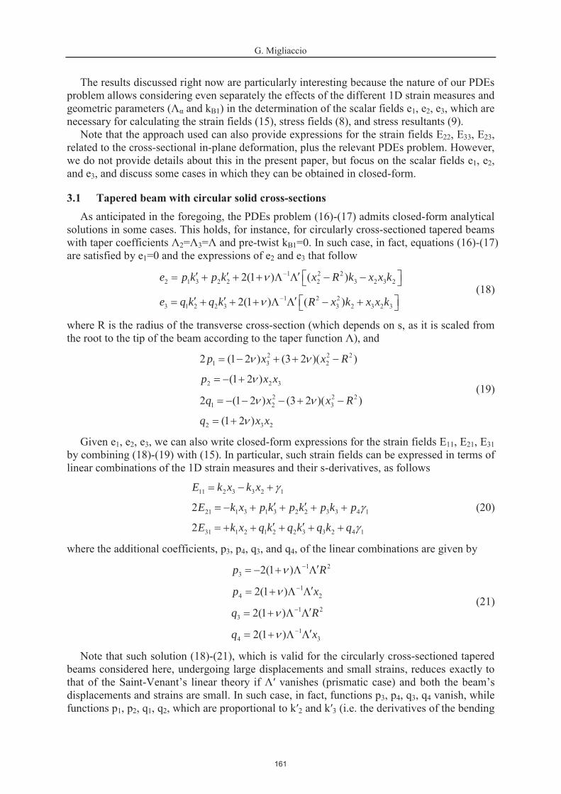
G. Migliaccio
The results discussed right now are particularly interesting because the nature of our PDEs problem allows considering even separately the effects of the different 1D strain measures and geometric parameters (Λα and kB1) in the determination of the scalar fields e1, e2, e3, which are necessary for calculating the strain fields (15), stress fields (8), and stress resultants (9).
Note that the approach used can also provide expressions for the strain fields E22, E33, E23,related to the cross-sectional in-plane deformation, plus the relevant PDEs problem. However, we do not provide details about this in the present paper, but focus on the scalar fields e1, e2,and e3, and discuss some cases in which they can be obtained in closed-form.
3.1 Tapered beam with circular solid cross-sections As anticipated in the foregoing, the PDEs problem (16)-(17) admits closed-form analytical
solutions in some cases. This holds, for instance, for circularly cross-sectioned tapered beamswith taper coefficients Λ2=Λ3=Λ and pre-twist kB1=0. In such case, in fact, equations (16)-(17) are satisfied by e1=0 and the expressions of e2 and e3 that follow
1 2 22 1 3 2 2 2 3 2 3 2
1 2 23 1 2 2 3 3 2 3 2 3
2(1 ) ( )
2(1 ) ( )
e p k p k x R k x x k
e q k q k R x k x x k(18)
where R is the radius of the transverse cross-section (which depends on s, as it is scaled from the root to the tip of the beam according to the taper function Λ), and
2 2 21 3 2
2 2 3
2 2 21 2 3
2 3 2
2 (1 2 ) (3 2 )( )
(1 2 )
2 (1 2 ) (3 2 )( )
(1 2 )
p x x R
p x x
q x x R
q x x
(19)
Given e1, e2, e3, we can also write closed-form expressions for the strain fields E11, E21, E31by combining (18)-(19) with (15). In particular, such strain fields can be expressed in terms of linear combinations of the 1D strain measures and their s-derivatives, as follows
11 2 3 3 2 1
21 1 3 1 3 2 2 3 3 4 1
31 1 2 1 2 2 3 3 2 4 1
2
2
E k x k x
E k x p k p k p k p
E k x q k q k q k q
(20)
where the additional coefficients, p3, p4, q3, and q4, of the linear combinations are given by 1 2
3
14 2
1 23
14 3
2(1 )
2(1 )
2(1 )
2(1 )
p R
p x
q R
q x
(21)
Note that such solution (18)-(21), which is valid for the circularly cross-sectioned tapered beams considered here, undergoing large displacements and small strains, reduces exactly to that of the Saint-Venant’s linear theory if Λʹ vanishes (prismatic case) and both the beam’s displacements and strains are small. In such case, in fact, functions p3, p4, q3, q4 vanish, while functions p1, p2, q1, q2, which are proportional to kʹ2 and kʹ3 (i.e. the derivatives of the bending
161

G. Migliaccio
curvatures), turn out to be proportional to the cross-sectional shear forces in the beam’s refer-ence state, as in the works of Timoshenko [12] and Sokolnikoff [13].
It is worth noting that similar but generally more complex expressions for E11, E21, E31 can be obtained for other non-prismatic beams as well (see, e.g., [6,21]). However, we do not dis-cuss here all cases in which we can obtain closed-form solutions to problem (16)-(17), but we present another interesting example (in section 3.2) and then proceed to compare the results of our model with those of nonlinear 3D-FEM simulations to verify its effectiveness in terms of computational efficiency and accuracy (section 4).
Before doing this, we remark that regardless of the approach used (i.e. numerical or analyt-ical) to solve our problem (16)-(17), the solution can always be expressed in terms of linear combinations of terms proportional to the 1D strain measures and their s-derivative, similarly to (18)-(20). The difference between the solution reported in this section and that of a generic bi-tapered, pre-twisted beam is represented by the expressions of the coefficients of the linear combinations (e.g. p1-p4), which are the functions of xα to be found. Such functions, however, have to be computed only once for a given cross-sectional shape. This fact, of course, con-tributes reducing the computational effort required to solve the nonlinear elasticity problem that governs the behavior of our three-dimensional beams, as is shown in section 4 via numer-ical examples and comparisons with the results of nonlinear 3D-FEM analyses.
3.2 Tapered beam with circular hollow cross-sections Let us now consider a tapered beam similar to that of the previous section, but having hol-
low cross-sections. Specifically, here we are considering thin-walled cross-sections, charac-terized by small thickness-to-radius ratio, t/R. For example, we can refer to the case in Figure 2, but without prescription on the shape of the taper function Λ (which does not need to be alinear function for the derivation of the following formulas).
Figure 2: Tapered beam with circular hollow cross-sections (right) and its taper coefficient (left)
Regarding functions e1, e2, e3 for the present beam, a vanishing e1 still satisfies the PDEs problem (16)-(17), but the expressions of e2, e3 obtained for the circular solid cross-sections insection 3.1 do not satisfy all PDEs and boundary conditions (16)-(17) of the present case. For their determination, apart from using a numerical method, we can exploit, here, a simplified analytical approach (common for thin-walled beams) based on the assumption that the strain and stress fields may not vary too much through the cross-sectional thickness.
162

G. Migliaccio
By using such approach, we proceed to derive formulas for the strain fields (15) valid for the present beam subject to flexure and express such formulas as functions of the bending curvatures and their s-derivatives. To this end, it is convenient to consider the components E11,Eθ1, Er1 of E (in place of E11, E21, E31), r and θ being the independent variables along the radial and tangential directions in the cross-section (see, e.g., Figure 2). Moreover, we also introduce the mean value Eθ, through the cross-sectional thickness t, of the tangential shear strain Eθ1,which is given by the following line-integral through the thickness
21 311 sin cos
tickness
E E Et
(22)
By exploiting (22), (15)-(16), and standard integration techniques based on Green’s formu-las, we can write Eθ in the following form
1 2 1 23 3 2 2(1 )( 3 ) sin (1 )( 3 ) cosE k k R k k R (23)
The mean value Er of the radial shear strain Er1 is instead obtained by exploiting the condi-tion of zero traction on the beam’s lateral surface, which yields
2 12 3(1 )( sin cos )rE k k R (24)
Now, the approximation relies on considering the local strain fields almost coincident with their mean value over the cross-sectional thickness, i.e. Eθ1≃Eθ and Er1≃Er. Such assumption is expected to provide good results in terms of predictions of the cross-sectional strain and stress fields in thin-walled tapered beams, the cross-sectional thickness of which is small with respect to the cross-sectional diameter or radius (e.g. t/R≃0.1).
The following examples provide comparisons with the results of nonlinear 3D-FEM simu-lations to verify the effectiveness of the modeling approach and formulas discussed so far.
4 APPLICATION EXAMPLES In this section we shows the results obtainable by our model, which we have implemented
in a numerical code written in Matlab language, referred to here as 3D-BLM. The results from 3D-BLM in terms of displacement, strain and stress fields are compared to those of nonlinear 3D-FEM analyses performed with Ansys, based on a fine mesh of solid tetrahedral elements with ten nodes and quadratic displacement behavior [24].
Two test cases are reported here. The first addresses a tapered beam with circular solid cross-sections, which may undergo large displacements while fixed at one end (the root) and loaded at the other (the tip) by a transverse force of progressively increasing magnitude. For such case we can exploit the analytical results presented in section 3.1. The second test case issimilar to the first, but the transverse cross-sections are hollow. For such case we exploit the formulas presented in section 3.2.
4.1 Test case 1 (solid cross-sections) The tapered beam considered here has a straight, 100m long centre-line; its transverse
cross-sections are circular, with a radius R=2m at the root, which is linearly scaled toward the tip up to 30% of the root value. The material properties are given in terms of Young’s modu-lus, 70GPa, and Poisson’s ratio, 0.25. The beam is fixed at the root and loaded at the tip by a flapwise dead force, F, ranging from 100kN to 15000kN (as in Figure 3). The simulation re-sults are summarized in the following.
163
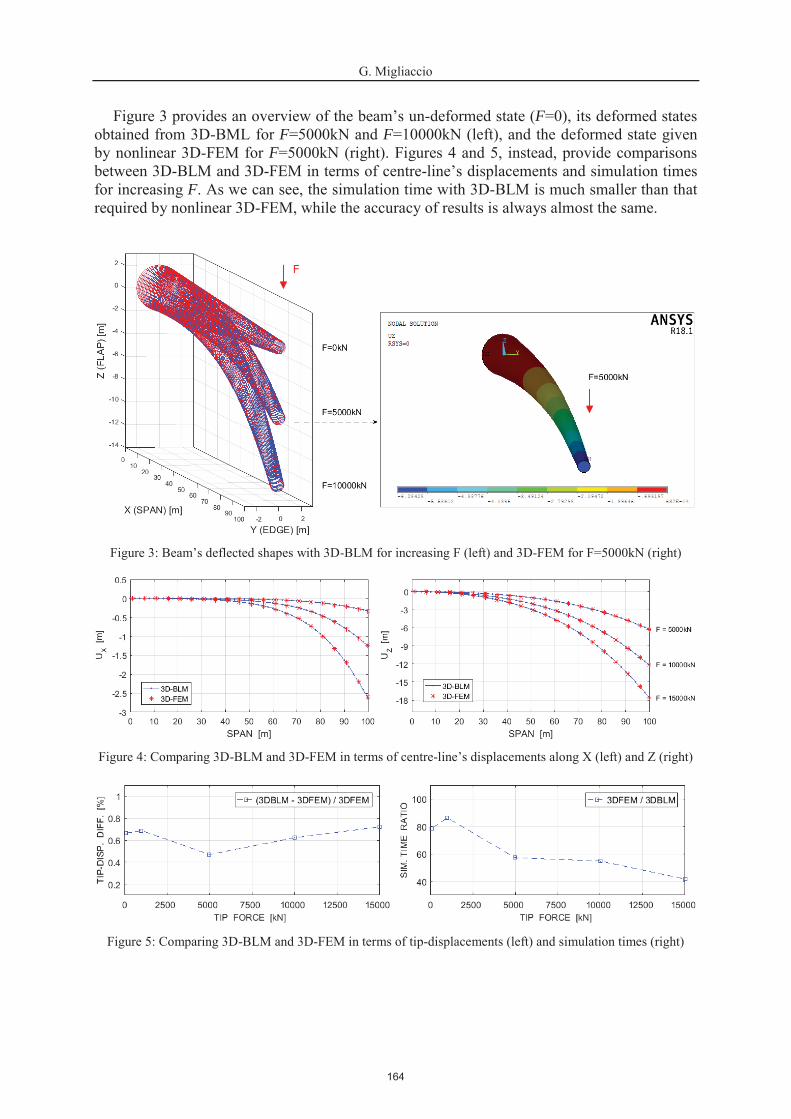
G. Migliaccio
Figure 3 provides an overview of the beam’s un-deformed state (F=0), its deformed states obtained from 3D-BML for F=5000kN and F=10000kN (left), and the deformed state given by nonlinear 3D-FEM for F=5000kN (right). Figures 4 and 5, instead, provide comparisons between 3D-BLM and 3D-FEM in terms of centre-line’s displacements and simulation times for increasing F. As we can see, the simulation time with 3D-BLM is much smaller than thatrequired by nonlinear 3D-FEM, while the accuracy of results is always almost the same.
Figure 3: Beam’s deflected shapes with 3D-BLM for increasing F (left) and 3D-FEM for F=5000kN (right)
Figure 4: Comparing 3D-BLM and 3D-FEM in terms of centre-line’s displacements along X (left) and Z (right)
Figure 5: Comparing 3D-BLM and 3D-FEM in terms of tip-displacements (left) and simulation times (right)
164

G. Migliaccio
Apart from this, our model can also provide other useful information about the mechanical behavior of our beam, e.g. the rotation of its local triads, its curvature change and strain fields,as well as the corresponding stress fields and stress resultants.
Figure 6, for example, reports the rotation θY of the local triads about Y, along with the curvature change about Y (kY), for increasing F. It is worth noting that the spanwise variation of the bending curvature kY is quite different from a linear function. However, this is expected for tapered beams (in spite of what would happen in a prismatic case under the same loading condition). This depends, in fact, on the spanwise variation of the cross-sectional bending stiffness which, in the present case, increases from the beam’s tip to the root according to the increasing cross-sectional diameter.
Figure 6: Local triads rotation θY (left) and bending curvature kY (right) with 3D-BLM for increasing F
As anticipated in the foregoing, 3D-BLM can also directly furnish the stress fields in all points of the beam. Hereafter we compare the results obtained in terms of Cauchy stress fieldsfrom 3D-BLM with those given by nonlinear 3D-FEM simulations.
Specifically, Figures 7 and 8 show the stress fields CXX and CZX obtained for F=100kN at three reference cross-sections (30%, 50%, 70% span). For completeness’ sake, we also report the results obtained for a much larger value of F (see Figures 9 and 10, F=10000kN). Similar results have moreover been obtained at other cross-sections and for other values of F.
Taking a look at the results obtained, we have observed that the normal stresses follow aNavier-like distribution in each cross-section (i.e. they are almost linear in x3), while the shear stress distributions are quite different from those predictable by the linear theory of prismatic beams. In fact, the transverse shear stresses at the cross-section’s boundary do not generally vanish in non-prismatic beams, while they are always zero in the prismatic case. Also, they can change from cross-section to cross-section in non-prismatic elements, while their distribu-tion and magnitude do not change spanwise in the prismatic case.
Figure 7: Stress field CXX at different cross-sections (30%, 50%, 70% span) for F=100kN
165

G. Migliaccio
Figure 8: Stress field CZX at different cross-sections (30%, 50%, 70% span) for F=100kN
Figure 9: Stress field CXX at different cross-sections (30%, 50%, 70% span) for F=10000kN
Figure 10: Stress field CZX at different cross-sections (30%, 50%, 70% span) for F=10000kN
The results obtained so far confirm the effectiveness of the modeling approach introduced in the foregoing and the accuracy of the closed-form solution of section 3.1.
4.2 Test case 2 (hollow cross-sections) The second test case considered here addresses a straight beam with 100m long centre-line
and circularly shaped hollow cross-sections, which are tapered from the root to the tip of the beam. The radius of the hollow root section is R=2m, while its thickness is t=0.2m. Such di-mensions are linearly reduced toward the beam’s tip as shown in Figure 2. The material prop-erties are summarized by reference values of Young’s modulus, 70GPa, and Poisson’s ratio, 0.25. The beam is fixed at the root and loaded at the tip by a flapwise dead force, F, ranging from 100kN to 10000kN (as in Figure 11).
166
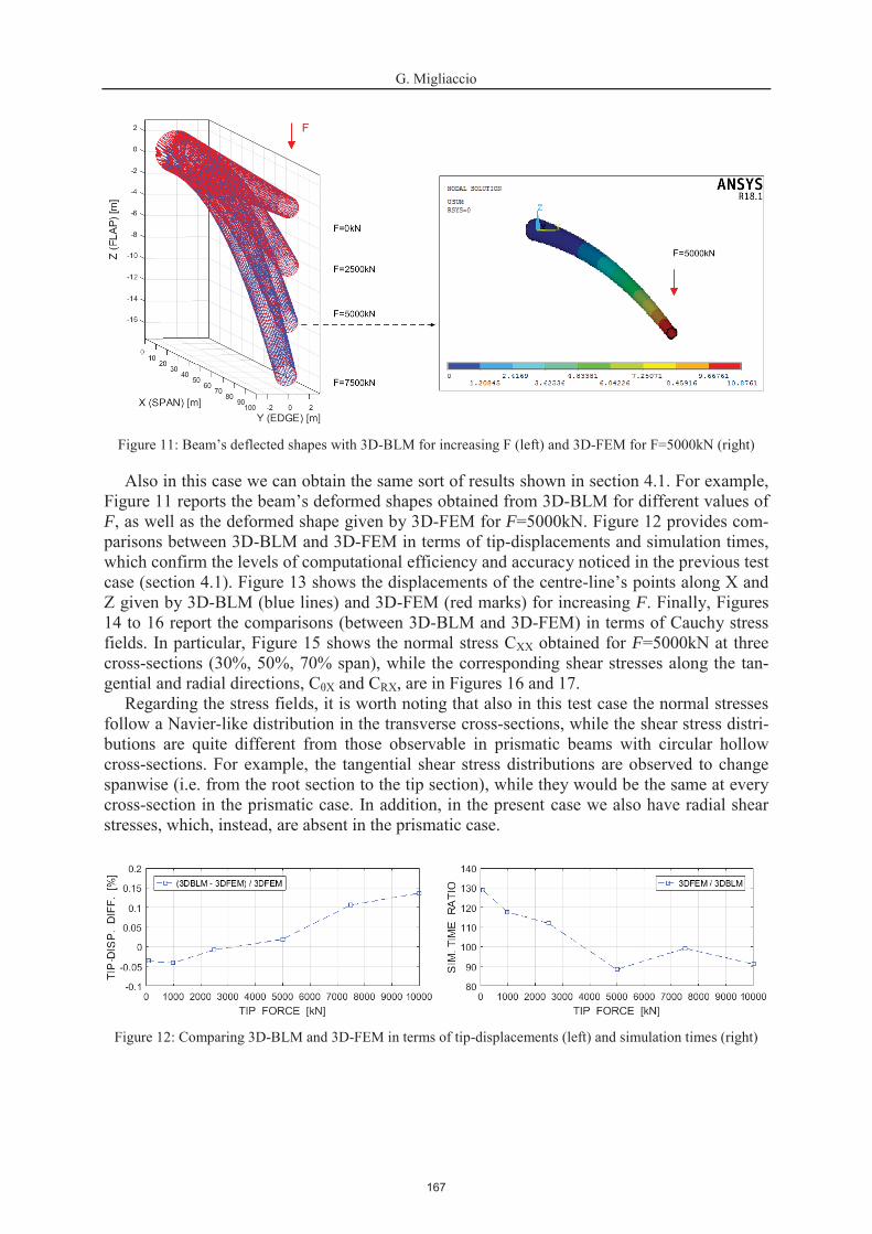
G. Migliaccio
Figure 11: Beam’s deflected shapes with 3D-BLM for increasing F (left) and 3D-FEM for F=5000kN (right)
Also in this case we can obtain the same sort of results shown in section 4.1. For example, Figure 11 reports the beam’s deformed shapes obtained from 3D-BLM for different values of F, as well as the deformed shape given by 3D-FEM for F=5000kN. Figure 12 provides com-parisons between 3D-BLM and 3D-FEM in terms of tip-displacements and simulation times, which confirm the levels of computational efficiency and accuracy noticed in the previous test case (section 4.1). Figure 13 shows the displacements of the centre-line’s points along X and Z given by 3D-BLM (blue lines) and 3D-FEM (red marks) for increasing F. Finally, Figures 14 to 16 report the comparisons (between 3D-BLM and 3D-FEM) in terms of Cauchy stress fields. In particular, Figure 15 shows the normal stress CXX obtained for F=5000kN at three cross-sections (30%, 50%, 70% span), while the corresponding shear stresses along the tan-gential and radial directions, CθX and CRX, are in Figures 16 and 17.
Regarding the stress fields, it is worth noting that also in this test case the normal stresses follow a Navier-like distribution in the transverse cross-sections, while the shear stress distri-butions are quite different from those observable in prismatic beams with circular hollowcross-sections. For example, the tangential shear stress distributions are observed to change spanwise (i.e. from the root section to the tip section), while they would be the same at every cross-section in the prismatic case. In addition, in the present case we also have radial shear stresses, which, instead, are absent in the prismatic case.
Figure 12: Comparing 3D-BLM and 3D-FEM in terms of tip-displacements (left) and simulation times (right)
167

G. Migliaccio
Figure 13: Comparing 3D-BLM and 3D-FEM in terms of displacements along X (left) and Z (right)
Figure 15: Stress field CXX at different cross-sections (30%, 50%, 70% span) for F=5000kN
Figure 16: Stress field CθX at different cross-sections (30%, 50%, 70% span) for F=5000kN
Figure 17: Stress field CRX at different cross-sections (30%, 50%, 70% span) for F=5000kN
The results shown in this example, which are based on the formulas derived in section 3.2, confirm once again the effectiveness of our modeling approach in terms of computational ef-ficiency and accuracy with respect to nonlinear 3D-FEM approaches. Other examples can also be found in previous works (e.g. [6,8,21]), which address other geometries and load cases.
168

G. Migliaccio
5 CONCLUSIONS Non-prismatic beamlike bodies are characterized by non-uniform cross-sections, yielding
stress distributions not predicable via prismatic beam theories and requiring non-prismatic beam models. This paper has illustrated a modeling approach for non-prismatic beams subject to large displacements, 3D cross-sectional warpings and small strains. Specifically, it provides a computationally efficient and accurate model that accounts for the main geometric features of such elements (e.g. taper) and provides the stress fields as linear combinations of 1D strain measures and geometric parameters, with the coefficients of such linear combinations to be computed only once for a given cross-sectional shape as solutions of PDEs, a fact which helps reducing the computational effort required to solve the 3D nonlinear problem.
Two test cases have been presented to illustrate how the model can be used and which re-sults it can provide. Analytical results have also been obtained, have been included in the nu-merical version of the model (3D-BLM) and have been compared with the results of nonlinear 3D-FEM analyses, confirming the efficiency and accuracy of the approach. Apart from the most theoretical outcomes of the model, it can be particularly useful for the design and opti-mization of non-prismatic elements used in engineering: in particular, on the one hand the closed-form formulas obtainable from the model can help an engineer since the preliminary design tasks; on the other hand, the model implemented in a numerical code can be used for multi-objective optimization tasks thanks to its computational efficiency and accuracy.
The results presented in this paper in terms of stress and strain fields have addressed the cross-sectional out-of-plane deformations and the corresponding PDEs. Investigations about the in-plane deformations and their PDEs would also be important, along with an analytical study about the effects of other geometric features (e.g. centre-line curvature) and those of the material non-homogeneity and anisotropy. An overview of other geometries that admit analyt-ical closed-form solutions would also be interesting, plus other numerical examples validating the proposed modeling approach against other geometries and load cases. All such topics will be addressed in subsequent works.
REFERENCES [1] Goodier G.N. and Griffin D.S., Elastic bending of pretwisted bars, Int. J. Solids Struc-
tures, 5, 1231-1245, 1969.
[2] Krenk S., The torsion-extension coupling in pretwisted elastic beams, Int. J. Solids Structures, 19, 67-72, 1983.
[3] Rosen A., Theoretical and experimental investigation of the nonlinear torsion and ex-tension of initially twisted bars, J. Applied Mechanics, 50, 321-326, 1983.
[4] Rosen A., Structural and dynamic behavior of pretwisted rods and beams, American So-ciety of Mechanical Engineers, 44, 483-515, 1991.
[5] Kunz D.L., Survey and comparison of engineering beam theories for helicopter rotor blades, J. of Aircraft, 31, 473-479, 1994.
[6] Migliaccio G., Ruta G., The influence of an initial twisting on tapered beams undergo-ing large displacements, Meccanica, 1-15, https://doi.org/10.1007/s11012-021-01334-2,2021.
[7] Buckney N., Pirrera A., et al., On the structural topology of wind turbine blades, Thin-Walled Structures, 67, 144-154, 2013.
169

G. Migliaccio
[8] Migliaccio G., Ruta G., et al., Beamlike models for the analyses of curved, twisted and tapered horizontal-axis wind turbine (HAWT) blades undergoing large displacements, Wind Energy Science, 5, 685-698, https://doi.org/10.5194/wes-5-685-2020, 2020.
[9] Migliaccio G., and Ruta G., Rotor blades as curved, twisted, and tapered beam-like structures subjected to large deflections, Engineering Structures, 222, 111089, 2020.
[10] Balduzzi G., Hochreiner G., and Füssl J., Stress recovery from one dimensional models for tapered bi-symmetric thin-walled I beams: deficiencies in modern engineering tools and procedures, Thin-Walled Structures, 119, 934-945, 2017.
[11] Love A.E.H., A treatise on the mathematical theory of elasticity, 4th ed., Dover Publica-tions, NY, 1944.
[12] Timoshenko S.P., Goodier J.N., Theory of elasticity, 2nd ed., McGraw-Hill, 1951.
[13] Sokolnikoff I.S., Mathematical theory of elasticity, 1st ed., McGraw-Hill Inc., 1946.
[14] Simo J.C., A finite strain beam formulation, the three-dimensional dynamic problem, part I, Computer methods in applied mechanics and engineering, 49, 55-70, 1985.
[15] Ibrahimbegovic A., On finite element implementation of geometrically nonlinear Reiss-ner’s beam theory: three-dimensional curved beam elements, Computer methods in ap-plied mechanics and engineering, 122, 11-26, 1995.
[16] Berdichevsky V.L., On the energy of an elastic rod, J. Appl. Mathematics and Mechan-ics, 45, 518-529, 1981.
[17] Yu W., Hodges D.H., and Ho J.C., Variational asymptotic beam-sectional analysis - an updated version, Int. J. Engineering Science, 59, 40-64, 2012.
[18] Migliaccio G., Ruta G, et al., Curved and twisted beam models for aeroelastic analysis of wind turbine blades in large displacements, XXIV AIMETA conference 2019, Lecture notes in mechanical engineering, Springer, 2020.
[19] Pai P.F., Three kinematic representations for modelling of high flexible beams and their applications, Int. J. Solids and Structures, 48, 2764-2777, 2011.
[20] Ruta G., Pignataro M., Rizzi N., A direct one-dimensional beam model for the flexural-torsional buckling of thin-walled beams, J. Mechanics of Materials and Structures, 1,1479-1496, 2006.
[21] Migliaccio G., Non-prismatic beamlike structures with 3D cross-sectional warping, in14th World Congress in Computational Mechanics (WCCM) & ECCOMAS congress 2020, Paris, France, 11-15 Jan. 2021.
[22] Gurtin M.E., An introduction to continuum mechanics, Mathematics in Science and En-gineering, 1st ed., Academic Press, 1981.
[23] Courant R., and Hilbert D., Methods of mathematical physics, 1st ed., Interscience Pub-lisher, 1953.
[24] Madenci E., and Guven I., The finite element method and applications in engineering using Ansys, 2nd ed., Springer, 2015.
170

ASSESSMENT OF MULTI-OBJECTIVE AND COEVOLUTIONARYGENETIC PROGRAMMING FOR PREDICTING THE STOKES FLOW
AROUND A SPHERE
Heiner Zille1, Fabien Evrard1, Julia Reuter1, Sanaz Mostaghim1, Berend van Wachem1
1Otto von Guericke University MagdeburgUniversitatsplatz 2, 39106 Magdeburg, Germany
e-mail: {firstname.lastname}@ovgu.de
Keywords: Genetic Programming, Fluid Dynamics, Multi-objective Optimization, Cooperative
Coevolution
Abstract. Genetic Programming (GP) has been used in a variety of fields to learn the rela-tionships between physical measurements of real-world problems. In this article, we combinedifferent techniques from the area of evolutionary optimization and, particularly, GP to solve afluid-dynamics problem: the Stokes flow around a rigid sphere. This serves as the starting pointto explore the potential of applying different GP techniques to such complex physical problems.From the definition of the considered fluid-dynamics problem, six benchmark instances withdifferent lengths and complexities are derived. We use single- and multi-objective GP methodsand compare their performance using different objective functions. More precisely, we studyhow model complexity, correlation and the consistency with physical laws (i.e. physical unitsof measurement) can be included as different objective functions, and whether their inclusionis beneficial to the overall search process. In addition, we include the concept of Coopera-tive Coevolution, which maintains multiple independent populations of solutions, into our GPimplementations and explore the capabilities and limitations of such coevolution-based opti-mization. We further propose a novel multi-phase approach, which alternates in the GP processbetween phases of traditional optimization and a mutation-only phase to reduce the model com-plexity. The results indicate that using multi-objective optimization is beneficial to the searchprocess and can help finding numerically correct solutions to the problems, especially when in-cluding a transformed Spearman correlation as an additional optimization goal. Furthermore,the inclusion of the physical units of measurement also helps guide the GP toward numericallycorrect and physically meaningful equations. While the concept of coevolution did not lead to asuperior performance in all cases, the precomputation of additional features, and the resultingreduction of the function set of the GP, leads to a drastic increase in performance and enablesthe algorithms to solve even the most complex of our benchmark instances. In the future, weaim to extend this research to more complex flows with multiple spheres and at higher Reynoldsnumbers, which involve a large number of input features.
171

Heiner Zille, Fabien Evrard, Julia Reuter, Sanaz Mostaghim, Berend van Wachem
1 INTRODUCTION
GP has been applied to a variety of applications to relate the physics of real-world phenom-
ena to their experimental measurements or numerical simulations. Typically in physics and
engineering applications, the goal of the optimization is not only to numerically predict vari-
ables accurately, but also to gain insight into the underlying physics and relations between input
variables. In that regard, the fact that GP produces human-readable mathematical models is
an advantage compared to other approaches such as Neural Networks (NN). In this article, we
combine different techniques from the area of multi-objective evolutionary optimization and
GP to solve a classical fluid-dynamics problem: the Stokes flow around a rigid sphere.
The fluid flow around a fixed rigid sphere is governed by a set of non-linear partial differ-
ential equations, the Navier-Stokes (NS) equations, and its nature depends upon the Reynolds
number, Re, a dimensionless quantity characterizing the ratio of inertial effects over viscous
effects within the fluid. Owing to the non-linearity of the NS equations, there is no general
analytical solution to this fluid-dynamics problem. However, when Re → 0 (also referred to as
the Stokes limit, or Stokes flow) the NS equations can be approximately linearized, and an ana-
lytical solution to the steady-state flow over a sphere of radius a, subject to the far-field velocity
u∞, can be derived [20]. The streamlines of this flow are shown in Fig. 1.
The application of GP to this fundamental flow problem serves as a starting point for ex-
ploring the capabilities of different GP techniques in predicting the behavior of complex flows,
such as particle-laden flows. To that end, we derive in this work six test problem instances
with different lengths and complexities, as to benchmark and compare different GP approaches
and their ability to recover the analytical expression of this flow. Four different algorithm vari-
ants using classical methods as well as techniques from the field of coevolutionary optimization
methods are compared. In the field of evolutionary optimization, the co-evolution of different
components of the solutions has become increasingly popular in recent years, and this concept
has also been applied to GP [e.g. 19]. In addition to using the concept of Cooperative Coevolu-
tion (CC) and a special multi-Phase GP approach, we investigate the use of multiple objective
functions for the optimization. The single-objective fitness optimization is compared with 2-, 3-
and 4-objective versions of the different algorithms, resulting in 32 different algorithms to solve
the benchmark instances. As far as physical or engineering applications are concerned, a trained
model that explains the connection between input and output data should also be consistent with
the laws that govern their evolution. This means that, even though numerically correct predic-
tions can be obtained, for instance, by adding a length and a time, such solutions are not in line
with physical units and therefore of little value. For this reason, we additionally formalize the
consistency with the law of physics as an objective. We furthermore include the correlation and
complexity of the model as two objective functions. Our experiments also discuss the possible
influence of incorporating expert knowledge and the precomputation of features on the perfor-
mance of the GP process. The insights provided by this study serve as a basis for exploring the
capabilities of GP in solving complex fluid-dynamics problems.
The remainder of this article is organized as follows. In Section 2, we derive the Stokes flow
around a rigid sphere and discuss its utility for the modeling of particle-laden flows. In Sec-
tion 3, we briefly outline the basics of Genetic Programming and the approaches that have been
used in the literature so far with regard to Cooperative Coevolution and the inclusion of phys-
ical measurements in the GP process. Subsequently, in Section 4, we introduce our proposed
GP variants and the objective functions we use in the optimization process. The benchmark
instances and their corresponding function- and terminal sets are outlined in Section 5. Finally,
172

Heiner Zille, Fabien Evrard, Julia Reuter, Sanaz Mostaghim, Berend van Wachem
we shows the results of our experimental evaluation in Section 6, and the article is concluded in
Section 7.
2 THE STOKES FLOW AROUND A SPHERE
Flows that are laden with particles are at the heart of many natural processes and engineering
applications, ranging from the flow of sediments in river beds to the combustion of fuel and
biomass in furnaces. Understanding and predicting such processes typically require the devel-
opment of reduced models to estimate the hydrodynamics forces acting on a particle carried
within a flow, based on the averaged properties of that flow. When viscous effects dominate in-
ertial effects, the Reynolds number of a rigid spherical particle of radius a, subject to a far-field
flow with velocity u∞ (‖u∞‖ = u∞), satisfies
Re =2 a ρ u∞
μ 1 , (1)
where ρ and μ are the density and viscosity of the fluid, respectively. It this regime, it is possible
to derive an analytical solution of the flow around the sphere, which is axi-symmetric about the
direction of the far-field velocity. In a spherical coordinate system whose origin is the center
of the sphere, and whose zenith is aligned with u∞, this flow can be expressed in terms of the
stream-function
ψ(r, θ) = u∞ sin2 θ
(r2
2+
a3
4 r− 3 a r
4
), (2)
which results in the velocity field
ur(r, θ) =1
r2 sin θ
∂ψ
∂θ= u∞ cos θ
(1 +
a3
2 r3− 3 a
2 r
), (3)
uθ(r, θ) = − 1
r sin θ
∂ψ
∂r= −u∞ sin θ
(1− a3
4 r3− 3 a
4 r
). (4)
This, in turn, enables the direct calculation of the resultant of the fluid forces acting on that
particle [20], which reads
F = 6 π aμu∞ . (5)
As soon as inertial effects become significant or if other particles are present in the vicinity
of the particle under consideration, it becomes impossible to derive such an analytical solution,
and one must rely on the results of experiments or numerical simulations to estimate the fluid
forces acting on the particle. Owing to the human-readable nature of the models it produces,
GP has the potential to provide a new insight into the non-linear physics of the flow through
ensembles of particles at varying Reynolds number, and can therefore lead to the development
of better reduced models for studying the behavior of particle-laden flows. In the following
sections, and with the aim to explore this potential, we apply GP to the case of the Stokes
flow around a fixed rigid sphere and study its ability to recover the analytical expressions of its
velocity field, as given in Eqs. (3) and (4). The six benchmark instances that we derive from the
Stokes problem are described in detail in Section 5.
3 GENETIC PROGRAMMING AND RELATED WORK
Genetic Programming (GP) is a subfield of Evolutionary Algorithms (EA) and was popular-
ized by the work of Koza [9]. EA makes use of the Darwinian principle of survival of the fittest
173
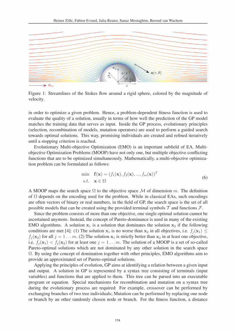
Heiner Zille, Fabien Evrard, Julia Reuter, Sanaz Mostaghim, Berend van Wachem
ex
ey
e r reθ
+θ
+
u(r, θ)
au∞
Figure 1: Streamlines of the Stokes flow around a rigid sphere, colored by the magnitude of
velocity.
in order to optimize a given problem. Hence, a problem-dependent fitness function is used to
evaluate the quality of a solution, usually in terms of how well the prediction of the GP model
matches the training data that serves as input. Inside the GP process, evolutionary principles
(selection, recombination of models, mutation operators) are used to perform a guided search
towards optimal solutions. This way, promising individuals are created and refined iteratively
until a stopping criterion is reached.
Evolutionary Multi-objective Optimization (EMO) is an important subfield of EA. Multi-
objective Optimization Problems (MOOP) have not only one, but multiple objective conflicting
functions that are to be optimized simultaneously. Mathematically, a multi-objective optimiza-
tion problem can be formulated as follows:
min f(x) = (f1(x), f2(x), ..., fm(x))T
s.t. x ∈ Ω(6)
A MOOP maps the search space Ω to the objective space M of dimension m. The definition
of Ω depends on the encoding used for the problem. While in classical EAs, such encodings
are often vectors of binary or real numbers, in the field of GP, the search space is the set of all
possible models that can be created using the provided terminal symbols T and functions F .
Since the problem consists of more than one objective, one single optimal solution cannot be
ascertained anymore. Instead, the concept of Pareto-dominance is used in many of the existing
EMO algorithms. A solution x1 is a solution that dominates the solution x2 if the following
conditions are met [4]: (1) The solution x1 is no worse than x2 in all objectives, i.e. fj(x1) ≤fj(x2) for all j = 1 . . .m. (2) The solution x1 is strictly better than x2 in at least one objective,
i.e. fj(x1) < fj(x2) for at least one j = 1 . . .m. The solution of a MOOP is a set of so-called
Pareto-optimal solutions which are not dominated by any other solution in the search space
Ω. By using the concept of domination together with other principles, EMO algorithms aim to
provide an approximated set of Pareto-optimal solutions.
Applying the principles of evolution, GP aims at identifying a relation between a given input
and output. A solution in GP is represented by a syntax tree consisting of terminals (input
variables) and functions that are applied to them. This tree can be parsed into an executable
program or equation. Special mechanisms for recombination and mutation on a syntax tree
during the evolutionary process are required: For example, crossover can be performed by
exchanging branches of two tree individuals; Mutation can be performed by replacing one node
or branch by an other randomly chosen node or branch. For the fitness function, a distance
174
Heiner Zille, Fabien Evrard, Julia Reuter, Sanaz Mostaghim, Berend van Wachem
measure between the produced and the desired output is often used such as the rooted mean
squared error.
In the basic version of GP, the execution of the program manipulates numerical values with-
out considering their physical units. This leads to situations in which non-physical solutions
can be produced; a result which is of little interest for physics or engineering applications. The
consideration of physical units inside GP was first proposed in [8], where special operators were
applied in order to repair incompatible units. As an example: an operation adding a length and
a time is repaired by artificially transforming a time into a length. This concept inspired mul-
tiple other works and has, since then, been implemented in single- as well as multi-objective
GP algorithms [e.g. 1, 15, 6]. A different development line in dimensionally aware GP focuses
on grammar-based GP, where constraints given by physical laws are already included in the
rules of the programming grammar [e.g. 14, 18]. Another noteworthy concept was presented
in [21], where strongly typed GP was used to generate viable method call sequences for soft-
ware testing. This approach limits the search space only to feasible solutions and could be
transferred to our problem by only allowing for dimensionally meaningful operations. A recent
work on dimensionally aware GP was presented in [12], where an approach similar to ours is
proposed: For each dimensionally incompatible GP operation, a penalty is calculated and ag-
gregated throughout an individual. Minimizing this penalty value is an additional objective of
the algorithm. Unlike the previously mentioned works, this method allows the initialization of
physically non-meaningful solutions and enables them to develop towards physically meaning-
ful solutions.
In most applications, GP has been used on a relatively small feature space, and research
on high-dimensional GP for regression problems remains sparse. Some work has been done
recently to include concepts like Cooperative Coevolution (CC) into the field of GP [e.g. 19],
which has been used in many evolutionary algorithms as a successful optimization technique
[e.g. 2, 23]. While CC, and more specifically the separation of solutions into multiple com-
ponents, has mostly been used in the EA community as a technique to solve high-dimensional
problems [22], CC-based approaches have been used in GP mostly as a way to boost per-
formance, irrespective of the number of features. Applying Cooperative co-evolutionary GP
(CCGP) on a problem requires (1) splitting the original feature space into smaller sets to cre-
ate subsolutions as well as (2) merging partial solutions into one combined solution. In [19],
the authors identified three different levels on which the merging of partial solutions in CCGP
can be performed: genotype, feature and ensemble level. While fusion on a genotype level is
the equivalent of the method originally proposed by Potter and De Jong [17] for evolutionary
algorithms, fusion on feature [10, 11] and ensemble level [5, 13, 16] have been studied more
extensively in the literature. The evaluation of the three proposed approaches on an image
denoising problem showed that the ensemble method performed best on the given task. The
authors also demonstrated that Cooperative coevolution can boost the performance of GP on
high-dimensional problems compared to other modern, non-CC GP approaches.
4 PROPOSED METHODS
In this work, we explore the potential of various combinations of GP-techniques for solving
Stokes Flow-related benchmarks. We use CC-based single- and multi-objective GP methods
and compare their performance using different objective functions. More precisely, we inves-
tigate how length, correlation and the consistency with physical laws (i.e. physical units of
measurement as, for instance, introduced in [8]) can be included as different objective func-
tions, and whether their inclusion is beneficial to the overall search process. In total, we use
175

Heiner Zille, Fabien Evrard, Julia Reuter, Sanaz Mostaghim, Berend van Wachem
four different variants of GP, along with 8 combinations of objective functions, which results
in 32 different optimization methods. In the following paragraphs, we start by describing the
four base-algorithm variants, before going into the details of the proposed objective function
combinations.
4.1 Algorithm Variants
Standard GP: The first algorithm used in this article is a standard GP algorithm, abbreviated
as S-GP, which is based on a classical (μ+ λ)-reproduction scheme and follows its implemen-
tation in the deap-framework1. The algorithm produces in each generation from a population
of size μ a set of λ offspring solutions, which are then evaluated. The best out of the (μ + λ)solutions are taken over to the next generation of the algorithm. This environmental selection
follows the procedure of the NSGA-II algorithm [3], while the selection of the parent-solutions
for the reproduction are chosen at random. The new λ solutions are created either by repeat-
edly recombining two random solutions from the current population, or by applying mutation
to a random individual. The mutation and recombination operators are selected at random from
different operators every time a recombination/mutation is carried out.
For recombination, the algorithm chooses between two crossover operators: One-point crossover
randomly selects a cut-off point in two individuals and swaps the selected branches. Leaf-based
one-point crossover does so as well, while giving higher probability to leaves being exchanged
between individuals rather than entire branches. For mutation, the algorithm chooses between
uniform mutation, node replacement, insertion mutation and shrink mutation, all of which are
chosen with equal probability. The uniform mutation replaces a randomly selected subtree by
a randomly generated new branch. Node replacement, as the name suggests, chooses one node
at random and replaces this function- or terminal-symbol with another one of the same arity.
The insertion mutation creates a new subtree and inserts it at a random position, using the pre-
vious branch on that position as a subcomponent of the created subtree. Shrink mutation aims
at decreasing the size of an individual by replacing a branch with one of its arguments.
Multi-Phase GP: The second algorithm is a Multi-Phase GP (MP-GP). The MP-GP is a vari-
ation of the S-GP above, which alternates between two phases of optimization behavior. In the
first phase, the algorithm behaves identically to the S-GP. In the second phase, the crossover op-
erators are disabled and the probabilities of the mutation operators to choose from are changed.
More precisely, in this second phase of the optimization, the algorithm only applies node re-
placement mutation and shrink mutation, where the former is chosen with a probability of 2/3and the latter with a probability 1/3. This two-stage approach avoids extensive growing of the
models and allows refinements through a frequent mutation of the population. This proves par-
ticularly useful since not all of the algorithm variants employ the length of the individual as an
objective, which in turn can lead to extensive growing of the trees. Another issue which was
often observed in initial experiments is that solutions which only differ from an optimal model
in one node may obtain a bad fitness, and using crossover is not likely to produce the required
small change. Moreover, the replacement of one node may have a large impact on the actual
fitness (for instance, changing an addition into a subtraction), which results in a less smooth
fitness landscape. Therefore, enabling the algorithm to perform this second phase with a focus
on small adjustments and shrinking the tree can be beneficial to find optimal solutions.
1https://github.com/DEAP/deap
176

Heiner Zille, Fabien Evrard, Julia Reuter, Sanaz Mostaghim, Berend van Wachem
Algorithm 1 Pseudocode of the Coevolutionary Genetic Programming (CC-GP)
Input: Training Data X , Terminals T , Functions F , Crossover probability pc, Mutation prob-
ability pm, Number of subpopulations vOutput: Set of non-dominated Solutions S
1: S0 ← Random initial population of Solutions for upper-level GP
2: r0 ← Choose random solution from S0 as representative
3: A0 ← Empty Pareto-dominance-based Archive
4: for i = 1 to v do5: Si ← Random initial population of Solutions for i−th lower-level GP
6: ri ← Choose random solution from Si as representative
7: Ai ← Empty Pareto-dominance-based Archive
8: end for9: repeat
10: for i = 1 to v do11: if i is part of r0 then12: Si, Ai ← Optimize Si using standard GP for k generations
13: ri ← updateRepresentative(Ai)
14: else15: ri ← Choose random solution from Si as representative
16: end if17: end for18: S0, A0 ← Optimize S0 using standard GP for k generations
19: r0 ← updateRepresentative(A0)
20: until total #Evaluations used
21: return⋃v
i=0 Ai
Cooperative-Coevolution-based GP: Our CC-based approach, abbreviated CC-GP, divides
the problem into multiple, independent populations, with the intent that each population could,
in theory, evolve different aspects of the original problem. As a result, multiple transformed fea-
tures are created which serve as inputs to another, higher-level GP process. Lower- and higher-
level GP populations are evolved cooperatively to enable the prediction of complex physical
relationships in the data. This means that function evaluations are only carried out coopera-
tively, by taking a representative from each of the lower-level and upper-level populations and
building a combined individual which is then evaluated using the training data.
The structure of the CC-GP algorithm is shown in Algorithm 1. In the main loop of the
algorithm, each lower-level population (sometimes also referred to as subpopulation) is evolved
using the standard GP method for a fixed amount of generations. After the last iteration of
each population’s optimization process, a representative solution is chosen from the current
population, and this representative is used in the subsequent function evaluations of the other
populations. After all lower-level populations have been evolved, the higher-level GP is used
to optimize models that represent combinations of the representatives of the lower-level pop-
ulations. The upper-level population uses only these representatives as input features, while
the lower-level populations operate on the terminal set and input features that are given by the
problem (i.e. that are also used in the above S-GP and MP-GP).
In order to use the computational budget more efficiently, the conditional statement of line
11 in Algorithm 1 is used to check whether the current, about-to-be-optimized subpopulation is
part of the current representative of the upper-level population. If that is not the case, then the
177
Heiner Zille, Fabien Evrard, Julia Reuter, Sanaz Mostaghim, Berend van Wachem
optimization of the lower-level population would be meaningless, since all function evaluations
would return the same values (as they only depend on the values of all other representatives).
Therefore, we assume that if a population i was not used in the current upper-level GP, the
feature that was given by the representative of subpopulation i may not have been useful, and
we replace it with a new, random representative.
Multi-Phase CC-GP: The last algorithm considered in this work, MP-CC-GP, is a combina-
tion of the two methods described above. It follows the same structure as the CC-GP, with the
addition that it also alternates between the two optimization phases. The switch between the
normal optimization (including crossover) and the mutation-only phase is done at the beginning
of the main loop, i.e. the algorithm optimizes each lower-level and the upper-level population
once with crossover and mutation, followed by one iteration with mutation only, as described
above.
4.2 Objective Function Specification
To examine the effect of different objective functions, and the benefit of using multi-objective
GP as opposed to a single-objective version, we define four different fitness functions. They
are related to the quality of the prediction, the correlation with the training data, the physical
correctness of the produced equations, and the complexity of the model. These four fitness
functions are used in different combinations in the experiments below.
Maximum Absolute Error (f1): The first objective function is related to the error between
the prediction of the GP-produced model and the actual, expected output in the data set. Since
we are interested in an accurate prediction of the physical relationship between the data, we
decided to use the maximum absolute error over the data set, i.e. during the training, the value
of f1 is the absolute error of the worst data point within the training data set. By using the
maximum error, we obtain a solution which guarantees that all predictions have at least a certain
quality. Preliminary experiments have shown that this leads more often to exact and physically
correct models compared to the rooted mean squared error.
Transformed Spearman Correlation (f2): The second objective function is a transformed
version of the Spearman Correlation ρ between the data set and the predictions. By using
this correlation coefficient to guide the optimization, the GP algorithm may favor models which
themselves are not numerically accurate, but are highly correlated with the desired output. Such
models can, for instance, be multiplicative or additive components within a numerically correct
model. A multi-objective EA optimizing f2 has the ability to keep such models in the population
over the generations, which can then be used in subsequent recombination steps to approximate
numerically correct results. As an example, the term u∞ · cos(θ) in Benchmark Instance 3 (see
below) would show a high correlation with the data set, even though the actual prediction of the
outcome ur may still be poor. An EA which optimizes with regard to f2, however, may consider
this as a good solution and keep it in the population for further refinement.
To utilize the correlation coefficient in the optimization, we transform its value to fit our
requirements. The range of ρ lies between -1 and 1, with a high coefficient indicating a strong
positive (non-linear or linear) correlation, and a low value of ρ indicates a strong negative cor-
relation. Both cases are, however, useful for the optimization, as building blocks with a strong
negative correlation may still be helpful when used in a subtraction, for instance. In addition, our
178

Heiner Zille, Fabien Evrard, Julia Reuter, Sanaz Mostaghim, Berend van Wachem
objective function are always minimized, which leads to a transformed objective f2 := 1− |ρ|.The worst possible value of f2 is 1.0, which indicates no correlation at all, while smaller values
of f2 indicate some kind of connection (positive or negative) between the model and the data
set.
In the CC-based approaches, a small adjustment is made to this objective: When the opti-
mization of one of the lower-level populations is carried out, the value of f2 is computed using
the output of only the current individual of the subpopulation (which represents only a branch
within the whole, combined tree model). In contrast, the upper-level GP uses the actual predic-
tion from the combined model (i.e. the model that incorporates all lower-level representatives
into the upper-level one). This way, the GP judges the features developed by the lower-level
GP processes based on how correlated this feature is with the target data, and therefore obtains
a more accurate measure of how useful the developed feature of this subpopulation is to the
whole, combined, CC-based optimization.
Dimension Penalty (f3): As explained previously in this article, it may be useful to guide the
optimization as to find physically correct models, which (1) do not violate the laws of physics in
their calculations and (2) predict the same unit of measurement as the unit of the target variable.
To achieve both of these goals, we model the third objective function f3 in the following way.
In our approach, contrary to the method used in [8], we do not use a special operator to
adjust units to each other. Instead, whenever incompatible units are used in an operator, the
operation is still carried out on the numerical values of the arguments, and the unit of the first
input argument is used as the unit of the result of the node (e.g. in case a length and a time
are added, the operation is carried out and the result is considered to be a length). To guide the
search towards evolving physically meaningful equations, a penalty value of 1.0 is added every
time such a nonphysical operation is carried out. This penalty value is accumulated along the
tree together with the outputs of each function node. As a result, the root of the tree returns a
value for the prediction of the training data, its physical units and a value for the total penalty
occurring in the execution of that tree. Since we know that the expected result is a model that
outputs, for instance, a velocity, any physical unit that is not expressed in meters/secondis not meaningful for the purpose of the application. Therefore, an additional penalty based
on the difference between the obtained units of the tree and the expected units of the output is
added. This additional penalty is based on the distances between the exponents of the SI-base
units (plus the unit radian for angles in this work) of which the final unit is composed. As an
example, velocity can be written as m1 · s−1. If our model output a result in the units m2 · s3,
the distances in the respective exponents are summed up as |1 − 2| + | − 1 − 3| = 1 + 4 = 5.
The value of the objective function f3 is defined as the sum of the accumulated penalty during
tree executing and the dimension-penalty for not matching the correct output units.
Length of Individual (f4): The last of the four objective functions considers the length of
the model, i.e. the number of nodes (function and terminal symbols) that are used to represent
the model in its tree-based representation. This can be seen as a measure of the complexity
of the model in terms of necessary mathematical operations. In the literature, the length of
the solutions is often used in a weighted sum together with the fitness / error to avoid extensive
growth of the trees. In our approach, instead, we employ the length as its own objective function.
In the CC-based algorithms, the length refers to the length of the complete, combined individual,
i.e. the model that incorporates all lower-level trees into the upper-level one.
179

Heiner Zille, Fabien Evrard, Julia Reuter, Sanaz Mostaghim, Berend van Wachem
4.3 Conflicts of Objective Functions
In contrast to the usual assumption in multi-objective optimization that the objective func-
tions are somewhat in conflict with each other, this does not have to be the case between f1 and
f2. It is clear that the model which perfectly optimizes f1 will also produce an optimal value for
f2. This property may, however, not be true in earlier generations of the GP, since there exist op-
timal solutions with regard to f2 with very poor performance in f1. A similar expectation can be
formulated for the relation between f1 and f3, although conflict may be stronger between these
two functions. It is, on the one hand, clear that the optimal model for f1 may, most probably,
also be physically correct. This however is only true if there exists an actual physically correct
relationship between the variables, which does not have to be the case for all applications. On
the other hand, it is easy to construct solutions which are physically correct and match the units
of the target variable, but perform horribly in a numerical sense with regard to f1 and f2. In
conclusion, we can assume that there is, at least for sub-optimal solutions, a conflict between
all four objective functions, although we can expect the conflict to vanish, the closer the models
get to an optimal prediction of the data. It should also be noted that a vanishing conflict is, for
our application, desirable, since the objectives f2 and f4 are merely tools to guide the algorithm
to better solutions, while the objectives that are actually important for the application are f1 and
f3.
5 BENCHMARK INSTANCES, FUNCTION SET AND TERMINAL SET
From the definition of the fluid-dynamics problem described in Section 2, we derive six
problem instances with varying complexities, alongside with the used function and terminal
sets. In the following, besides the variables and derived features of the problem, the terminal
sets T include a set of constants, which we set as C = {4, 3, 2, 1, 12, 14}.
Benchmark Instance 1: Predict |u| from ux and uy.
|u| =√
u2x + u2
y (7)
Instance 1 is a rather simple equation and involves only 2 variables. To solve this in-
stance, 4 computational operations are necessary (two multiplications or square-operations,
one addition and one square root operation). The function set for this instance is given as
F = {+,−,×, ◦2, ◦3, 1◦ , sin(◦), cos(◦),√◦} and the terminal set as T = C ∪ {ux, uy}, where ◦denotes the input of the unary functions.
Benchmark Instance 2: Predict ux from ur, uθ and θ.
ux = ur · cos(θ)− uθ · sin(θ) (8)
Instance 2 is more complex, first due to its length (3 variables and 5 computational opera-
tions), but also due to the inclusion of trigonometric functions. Compared to the other unary
functions such as the square root, the power function or the multiplicative inverse, the trigono-
metric functions sin(◦) and cos(◦) are not monotonously increasing or decreasing with their
input argument. Therefore, the fitness landscape in this problem instance may be more com-
plex, and finding the optimal model to solve it may be more challenging for the GP variants.
The function set for this instance is given as F = {+,−,×, ◦2, ◦3, 1◦ , sin(◦), cos(◦)} and the
terminal set as T = C ∪ {ur, uθ, θ}.
180

Heiner Zille, Fabien Evrard, Julia Reuter, Sanaz Mostaghim, Berend van Wachem
Benchmark Instance 3: Predict ur from u∞, θ, a and r.
ur = u∞ · cos(θ) ·(1 +
a3
2 · r3 − 3 · a2 · r
)(9)
Instance 3 is the most complex and involves 4 variables and 13 computational operations
(given its function set F , defined below) in its simplified form as given in Equation (9). How-
ever, the GP may not necessarily end up with the simplification of multiplying the first two
terms after the addition and subtraction in the parenthesis, and the expanded form of this equa-
tion needs 19 operations. Instance 3 further involves a trigonometric function, which adds the
same additional complexity as described in Instance 2. The function and terminal sets for this
instance are F = {+,−,×, ◦2, ◦3, 1◦ , sin(◦), cos(◦)} and T = C ∪ {a, r, u∞, θ}.
Benchmark Instance 4: The basic relation between input and output variables in Instance 4
is identical to the one in Instance 1, i.e. the same equation needs to be learned. However, to
examine the effect of preprocessing variables using expert knowledge or other computational
techniques, we change the terminal and function sets compared to Instance 1. We use some
of the unary function operators in the original set F and perform their operation of the input
variables ux and uy. As a results, we obtain a smaller set of functions, but in exchange a
much larger set of terminal symbols for the GP process. The sets for Instance 4 are F ={+,−,×,
√◦} and T = C ∪ {ux, uy} ∪ {u2x, u
3x,
1ux, u2
y, u3y,
1uy}. Since we assume that the
functions sin(◦) and cos(◦) can only be applied to angles in order to be physically meaningful,
these two functions are not used on the velocities ux and uy. While the effect of a much larger
terminal set is explored in our experiments (see Section 6.4), from a theoretical point of view
Instance 4 is less complex than Instance 1, since only two operations are now necessary to
assemble the correct equation.
Benchmark Instance 5: Instance 5 follows the same equation as Instance 2, but with changed
function and terminal sets, as done in Instance 4. Again, trigonometric functions are applied
to angles, while the other functions are applied to the velocities. As a result, we obtain F ={+,−,×} and T = C ∪ {ur, uθ, θ} ∪ {u2
r, u3r,
1ur, u2
θ, u3θ,
1uθ, sin(θ), cos(θ)}.
Benchmark Instance 6: As done in Instances 4 and 5, we derive Instance 6 from the equation
of Instance 3 and change the function and terminal sets to F = {+,−,×} and T = C ∪{a, r, u∞, θ} ∪ {a2, a3, 1
a, r2, r3, 1
r, u2
∞, u3∞, 1
u∞ , sin(θ), cos(θ)}. As a result, while the terminal
set is much larger than that of Instance 3, the complexity in terms of the necessary number of
operations is smaller (10 operations).
For the above-mentioned benchmark instances, we create a data set of 366 data points using a
far-field velocity u∞ = 1.0 and a radius of the sphere of a = 1.0. The data set is randomly split
in an 80/20 ratio, i.e. into 292 data points in the training set and 74 data points in the test set.
6 EVALUATION
In conducting experiments, we aim to compare various aspects of the algorithms and to com-
pare the problems with each other. More precisely, we aim to answer the following questions:
181

Heiner Zille, Fabien Evrard, Julia Reuter, Sanaz Mostaghim, Berend van Wachem
1. How are the numerical performance and physical correctness of the results affected by
the inclusion of additional objectives, especially of correlation and dimension-penalty?
(Section 6.1)
2. How do the Cooperative Coevolution-based GP methods perform compared to the classi-
cal approaches? (Section 6.2)
3. How is performance affected by the multi-phase approach with additional mutation-only
phases? (Section 6.3)
4. How is performance affected by the precomputation of features, and the corresponding
changes in the function- and terminal-sets of the GP? (Section 6.4)
In this section, we answer these questions in detail by comparing the results of 32 combina-
tions of algorithms and fitness functions on the six benchmark instances described in Section 5.
The first objective function f1 is always part of the optimization, and is paired with all possi-
ble combinations of the other three objectives, as seen in Table 1. For each algorithm variant
and benchmark instance, we perform 31 independent runs. The parameters are set as follows:
The population size is μ = λ = 2000 for all algorithms. The probabilities for crossover and
mutation are set to 0.5 and 0.5 respectively, except in the Multi-phase approaches, where no
crossover is used and the mutation probability is set to 1.0 instead. The number of generations
before a switch between normal optimization and mutation-only phase is set to 20. In the CC-
based algorithms, all populations are optimized for 20 generations before moving on to the next
one, and a switch of the phase in the CC-MP-GP is done once all lower-level and the upper-
level GPs have been optimized once. The number of lower-level populations in CC-GP and
CC-MP-GP is set to 2. In the leaf-based one-point crossover the probability to select a terminal
symbol is set to 0.9. The maximum depth of the initial random solutions is set to 4. During
the optimization, created solutions are restricted to a maximum length of 50 for the S-GP and
the MP-GP, and a maximum length of 15 for the CC-based variants. The smaller limit in the
CC-based algorithms applies to each population, but the combination of the representatives to
form one final individual can, of course, still create much longer models. All experiments stop
after 1, 600, 000 function evaluations, i.e. after 800 generations of optimization. The algorithms
are implemented using the deap-framework2 version 1.3.1 [7] and the pint package3 version
0.16.1.
In order to examine the quality of solutions, Table 1 shows the results of the experiments in
terms of success rates, i.e. the numbers show how many out of the 31 runs achieved a certain
goal. We compare two different types of success rates:
1. The first number represents the physical and numerical success rate. It shows how many
runs have achieved a perfect numerical results, which we consider as f1 < 1e−15 and at
the same time delivered a model that satisfies f3 = 0 and therefore delivered the correct
units of measurement in a physically correct way.
2. The second number in each cell shows the numerical success rate only, i.e. how many
models delivered a maximum absolute error of f1 < 1e−15, regardless of an existing
dimension penalty in f3.
2https://github.com/DEAP/deap3https://github.com/hgrecco/pint
182

Heiner Zille, Fabien Evrard, Julia Reuter, Sanaz Mostaghim, Berend van Wachem
Objectives 1 2 3 4 5 6
S-GP
f1 - / - 1 / 1 - / - 30 / 31 2 / 4 - / 17
f1, f2 30 / 31 1 / 1 - / 5 31 / 31 3 / 5 - / 31
f1, f3 2 / 2 - / - - / - 31 / 31 18 / 18 7 / 7
f1, f4 - / - - / - - / - 31 / 31 10 / 10 - / -
f1, f2, f3 31 / 31 8 / 8 13 / 13 31 / 31 25 / 25 27 / 28
f1, f2, f4 31 / 31 - / - - / - 31 / 31 11 / 13 - / 4
f1, f3, f4 - / - - / - - / - 31 / 31 13 / 14 - / -
f1, f2, f3, f4 31 / 31 1 / 1 - / 1 31 / 31 29 / 29 - / 6
MP-GP
f1 - / - - / - - / - 28 / 30 3 / 4 - / 17
f1, f2 30 / 30 3 / 3 - / 3 31 / 31 3 / 5 - / 31
f1, f3 - / - - / - - / - 31 / 31 17 / 18 7 / 7
f1, f4 - / - - / - - / - 31 / 31 3 / 3 - / -
f1, f2, f3 30 / 30 6 / 6 4 / 7 31 / 31 25 / 25 22 / 22
f1, f2, f4 28 / 28 - / - - / - 31 / 31 4 / 4 - / -
f1, f3, f4 1 / 1 - / - - / - 31 / 31 2 / 2 - / -
f1, f2, f3, f4 31 / 31 - / - - / - 31 / 31 14 / 14 - / -
CC-GP
f1 1 / 1 - / - - / - 16 / 17 9 / 11 - / 1
f1, f2 29 / 31 - / - - / - 29 / 31 5 / 7 - / 8
f1, f3 4 / 4 - / - - / - 26 / 26 14 / 14 - / -
f1, f4 - / - - / - - / - 28 / 28 2 / 2 - / -
f1, f2, f3 27 / 27 6 / 6 - / - 29 / 29 24 / 24 2 / 3
f1, f2, f4 31 / 31 - / - - / - 31 / 31 5 / 8 - / -
f1, f3, f4 1 / 1 - / - - / - 22 / 22 11 / 12 - / -
f1, f2, f3, f4 28 / 28 - / 1 - / - 29 / 29 15 / 17 - / -
MP-CC-GP
f1 - / - - / - - / - 19 / 20 8 / 9 - / 3
f1, f2 30 / 31 - / - - / - 30 / 30 4 / 7 - / 9
f1, f3 2 / 2 - / - - / - 28 / 28 20 / 20 - / 1
f1, f4 2 / 2 - / - - / - 28 / 28 1 / 1 - / -
f1, f2, f3 28 / 28 5 / 5 - / - 29 / 30 21 / 21 - / 4
f1, f2, f4 30 / 30 2 / 2 - / - 29 / 29 3 / 4 - / -
f1, f3, f4 2 / 2 - / - - / - 21 / 21 4 / 4 - / -
f1, f2, f3, f4 29 / 29 - / - - / - 29 / 29 12 / 12 - / -
Table 1: Success rates for the six benchmark instances in terms of numerically and physically
correct results (first number) and numerically correct results only (second number). A value of
0 is shown as a dash.
In addition, we take a close look at the actual numerical results. Table 2 shows the average
values obtained for f1 over the 31 independent runs. For each of the benchmark instances
(each of the columns), the respective best performance is marked in bold. A one-sided Mann-
Whitney-U statistical test was performed for each algorithm to test whether its performance was
significantly worse than that of the respective best algorithm for that benchmark. A difference
is considered significant for p < 0.05 and is marked with an asterisk in Table 2, while all
non-significant results are printed in bold font.
All analyses in this section are performed on the test set, which was not available to the algo-
rithms during the optimization process. In general, the observed performance in all experiments
does not differ significantly between the test set and the training set, which indicates that none
of the algorithms suffers from a large amount of overfitting.
183

Heiner Zille, Fabien Evrard, Julia Reuter, Sanaz Mostaghim, Berend van Wachem
Ob
ject
ives
12
34
56
S-G
P
f1
4.3
7e-
03
*(±
4.2
3e-
03)
3.8
5e-
02
*(±
2.0
9e-
02)
2.1
8e-
02
*(±
1.3
9e-
02)
0.00
e+00
(±0.0
0e+
00)
5.0
0e-
02
*(±
3.0
0e-
02)
6.0
8e-
03
*(±
7.4
8e-
03)
f1,f
20.
00e+
00(±
0.0
0e+
00)
3.6
2e-
02
*(±
1.9
3e-
02)
2.0
9e-
03
*(±
2.5
2e-
03)
0.00
e+00
(±0.0
0e+
00)
5.0
3e-
02
*(±
2.9
9e-
02)
1.92
e-16
(±3.7
8e-
17)
f1,f
31
.09
e-0
2*
(±7.9
9e-
03)
6.5
4e-
02
*(±
3.0
4e-
02)
1.8
6e-
02
*(±
1.2
8e-
02)
0.00
e+00
(±0.0
0e+
00)
2.9
6e-
02
*(±
4.0
0e-
02)
1.4
4e-
02
*(±
9.9
9e-
03)
f1,f
41
.86
e-0
2*
(±1.4
9e-
03)
1.3
5e-
01
*(±
3.0
8e-
02)
1.5
5e-
01
*(±
2.6
7e-
02)
0.00
e+00
(±0.0
0e+
00)
7.5
5e-
02
*(±
5.4
1e-
02)
8.5
3e-
02
*(±
4.0
0e-
02)
f1,f
2,f
34
.03
e-1
8*
(±1.3
7e-
17)
1.46
e-02
(±2.0
0e-
02)
9.70
e-04
(±1.4
5e-
03)
0.00
e+00
(±0.0
0e+
00)
1.84
e-03
(±4.5
0e-
03)
5.78
e-04
(±1.7
8e-
03)
f1,f
2,f
43.
58e-
18(±
1.9
6e-
17)
8.6
1e-
02
*(±
2.4
3e-
02)
1.9
5e-
02
*(±
9.4
8e-
03)
3.58
e-18
(±1.9
6e-
17)
6.0
9e-
02
*(±
5.4
3e-
02)
3.7
0e-
02
*(±
2.1
1e-
02)
f1,f
3,f
41
.90
e-0
2*
(±2.0
7e-
03)
1.2
2e-
01
*(±
2.1
9e-
02)
1.3
3e-
01
*(±
3.6
9e-
02)
0.00
e+00
(±0.0
0e+
00)
5.5
2e-
02
*(±
5.5
2e-
02)
8.6
3e-
02
*(±
3.1
6e-
02)
f1,f
2,f
3,f
47.
16e-
18(±
3.9
2e-
17)
3.0
3e-
02
*(±
1.6
2e-
02)
9.3
4e-
03
*(±
6.9
0e-
03)
0.00
e+00
(±0.0
0e+
00)
1.01
e-03
(±4.3
1e-
03)
2.1
0e-
02
*(±
1.6
2e-
02)
MP
-GP
f1
5.2
7e-
03
*(±
4.1
2e-
03)
5.2
1e-
02
*(±
2.5
6e-
02)
2.2
6e-
02
*(±
2.9
1e-
02)
2.63
e-05
(±1.4
4e-
04)
5.0
5e-
02
*(±
2.6
0e-
02)
6.4
7e-
03
*(±
8.6
8e-
03)
f1,f
24.
44e-
17(±
2.2
4e-
16)
3.9
2e-
02
*(±
2.5
7e-
02)
2.5
8e-
03
*(±
2.5
8e-
03)
0.00
e+00
(±0.0
0e+
00)
5.4
2e-
02
*(±
2.7
3e-
02)
1.98
e-16
(±3.5
1e-
17)
f1,f
31
.51
e-0
2*
(±7.3
7e-
03)
1.0
0e-
01
*(±
3.2
4e-
02)
6.5
4e-
02
*(±
4.9
4e-
02)
0.00
e+00
(±0.0
0e+
00)
3.0
9e-
02
*(±
4.1
1e-
02)
1.6
5e-
02
*(±
1.3
8e-
02)
f1,f
42
.03
e-0
2*
(±3.8
1e-
03)
1.5
6e-
01
*(±
3.6
4e-
02)
1.5
7e-
01
*(±
2.4
2e-
02)
0.00
e+00
(±0.0
0e+
00)
1.1
1e-
01
*(±
4.3
1e-
02)
1.1
7e-
01
*(±
4.8
2e-
02)
f1,f
2,f
35
.97
e-0
5*
(±3.2
7e-
04)
2.5
2e-
02
*(±
2.4
9e-
02)
2.5
8e-
03
*(±
3.0
7e-
03)
0.00
e+00
(±0.0
0e+
00)
3.39
e-03
(±9.6
5e-
03)
1.9
6e-
03
*(±
3.5
3e-
03)
f1,f
2,f
41
.02
e-0
3*
(±3.8
1e-
03)
1.0
6e-
01
*(±
2.6
5e-
02)
3.4
1e-
02
*(±
1.3
6e-
02)
0.00
e+00
(±0.0
0e+
00)
1.0
0e-
01
*(±
4.0
9e-
02)
5.1
2e-
02
*(±
1.3
7e-
02)
f1,f
3,f
41
.86
e-0
2*
(±4.1
5e-
03)
1.4
2e-
01
*(±
2.9
8e-
02)
1.5
7e-
01
*(±
1.3
4e-
02)
0.00
e+00
(±0.0
0e+
00)
1.0
8e-
01
*(±
4.0
6e-
02)
9.2
4e-
02
*(±
4.2
2e-
02)
f1,f
2,f
3,f
40.
00e+
00(±
0.0
0e+
00)
5.5
2e-
02
*(±
2.8
2e-
02)
1.6
0e-
02
*(±
6.7
3e-
03)
0.00
e+00
(±0.0
0e+
00)
3.7
2e-
02
*(±
4.3
7e-
02)
4.2
0e-
02
*(±
1.7
0e-
02)
CC
-GP
f1
9.1
6e-
03
*(±
5.3
6e-
03)
7.2
7e-
02
*(±
3.3
0e-
02)
4.1
8e-
02
*(±
2.2
8e-
02)
2.3
5e-
02
*(±
1.0
4e-
01)
9.9
3e-
02
*(±
1.2
8e-
01)
8.3
4e-
02
*(±
1.1
6e-
01)
f1,f
22.
64e-
17(±
1.3
5e-
16)
4.3
1e-
02
*(±
1.9
6e-
02)
9.5
2e-
03
*(±
6.1
8e-
03)
1.07
e-17
(±4.3
3e-
17)
4.7
4e-
02
*(±
3.3
2e-
02)
1.6
1e-
02
*(±
3.7
8e-
02)
f1,f
31
.40
e-0
2*
(±6.6
3e-
03)
1.0
7e-
01
*(±
4.9
4e-
02)
8.5
4e-
02
*(±
3.8
7e-
02)
5.9
8e-
04
*(±
1.8
1e-
03)
6.5
9e-
02
*(±
7.9
1e-
02)
7.1
2e-
02
*(±
9.0
3e-
02)
f1,f
42
.07
e-0
2*
(±3.5
5e-
03)
1.5
3e-
01
*(±
3.4
7e-
02)
1.4
4e-
01
*(±
3.3
6e-
02)
2.1
5e-
03
*(±
7.4
3e-
03)
1.1
3e-
01
*(±
5.1
8e-
02)
8.7
7e-
02
*(±
5.2
8e-
02)
f1,f
2,f
36
.74
e-0
4*
(±2.1
7e-
03)
6.5
3e-
02
*(±
6.1
1e-
02)
1.9
2e-
02
*(±
1.3
0e-
02)
1.8
7e-
05
*(±
1.0
3e-
04)
1.0
8e-
02
*(±
2.7
8e-
02)
4.8
1e-
02
*(±
7.5
3e-
02)
f1,f
2,f
41
.61
e-1
7*
(±4.7
2e-
17)
9.8
5e-
02
*(±
2.0
8e-
02)
3.6
9e-
02
*(±
1.6
0e-
02)
3.58
e-18
(±1.9
6e-
17)
5.7
4e-
02
*(±
4.2
3e-
02)
5.2
3e-
02
*(±
3.9
7e-
02)
f1,f
3,f
41
.70
e-0
2*
(±7.1
9e-
03)
1.4
4e-
01
*(±
5.4
9e-
02)
1.2
7e-
01
*(±
3.2
8e-
02)
6.1
3e-
03
*(±
1.1
9e-
02)
1.0
1e-
01
*(±
1.1
6e-
01)
1.0
4e-
01
*(±
6.3
4e-
02)
f1,f
2,f
3,f
44
.24
e-0
4*
(±1.3
8e-
03)
5.1
4e-
02
*(±
4.0
4e-
02)
3.0
7e-
02
*(±
1.4
8e-
02)
1.1
5e-
04
*(±
5.7
5e-
04)
2.2
8e-
02
*(±
3.3
8e-
02)
7.9
3e-
02
*(±
1.0
3e-
01)
MP
-CC
-GP
f1
1.1
5e-
02
*(±
4.3
7e-
03)
6.9
2e-
02
*(±
2.7
4e-
02)
4.9
7e-
02
*(±
2.9
2e-
02)
4.0
5e-
02
*(±
1.4
5e-
01)
8.3
4e-
02
*(±
1.4
5e-
01)
4.0
7e-
02
*(±
6.1
1e-
02)
f1,f
21.
07e-
17(±
4.3
3e-
17)
4.2
3e-
02
*(±
1.4
4e-
02)
1.2
9e-
02
*(±
6.7
0e-
03)
1.7
5e-
04
*(±
9.5
7e-
04)
5.7
1e-
02
*(±
7.7
5e-
02)
1.0
7e-
02
*(±
9.3
2e-
03)
f1,f
31
.65
e-0
2*
(±6.4
5e-
03)
1.0
8e-
01
*(±
4.6
6e-
02)
9.1
8e-
02
*(±
4.3
5e-
02)
2.1
3e-
03
*(±
9.9
5e-
03)
4.4
6e-
02
*(±
1.0
2e-
01)
6.8
9e-
02
*(±
9.0
1e-
02)
f1,f
41
.88
e-0
2*
(±6.6
0e-
03)
1.5
3e-
01
*(±
4.7
9e-
02)
1.5
7e-
01
*(±
2.0
8e-
02)
1.7
5e-
03
*(±
5.3
6e-
03)
1.4
3e-
01
*(±
9.9
1e-
02)
1.2
0e-
01
*(±
7.4
1e-
02)
f1,f
2,f
34
.49
e-0
4*
(±1.8
3e-
03)
4.6
4e-
02
*(±
4.1
0e-
02)
2.3
0e-
02
*(±
1.6
2e-
02)
1.43
e-07
(±7.8
2e-
07)
4.9
3e-
02
*(±
1.1
9e-
01)
3.3
4e-
02
*(±
5.8
1e-
02)
f1,f
2,f
45.
93e-
04(±
3.2
5e-
03)
9.1
1e-
02
*(±
3.6
9e-
02)
4.4
4e-
02
*(±
1.9
7e-
02)
3.56
e-04
(±1.8
9e-
03)
7.8
4e-
02
*(±
4.4
3e-
02)
8.2
9e-
02
*(±
9.0
4e-
02)
f1,f
3,f
41
.82
e-0
2*
(±5.5
9e-
03)
1.7
2e-
01
*(±
4.2
1e-
02)
1.5
1e-
01
*(±
1.9
5e-
02)
7.1
2e-
03
*(±
1.1
2e-
02)
1.3
3e-
01
*(±
1.1
5e-
01)
1.2
6e-
01
*(±
9.1
7e-
02)
f1,f
2,f
3,f
41
.10
e-0
3*
(±4.1
8e-
03)
8.5
8e-
02
*(±
3.5
2e-
02)
3.6
1e-
02
*(±
1.5
0e-
02)
7.9
3e-
04
*(±
3.9
7e-
03)
3.1
5e-
02
*(±
7.6
9e-
02)
8.2
0e-
02
*(±
1.0
6e-
01)
Tab
le2:
Num
eric
alre
sult
s(a
ver
age
and
stan
dar
ddev
iati
on)
over
31
runs
for
the
six
ben
chm
ark
inst
ance
s.B
est
resu
lts
for
each
inst
ance
are
show
nin
bold
.A
stat
isti
call
ysi
gnifi
cant
dif
fere
nce
(p<
0.05
)is
indic
ated
wit
han
aste
risk
.
184

Heiner Zille, Fabien Evrard, Julia Reuter, Sanaz Mostaghim, Berend van Wachem
6.1 The Effect of Adding Additional Objectives
First, we take a look at how the final performance, numerically and physically, is impacted
by the inclusion of additional objectives.
The effect of f2: For the S-GP, we can see in Table 1 that the (f1, f2)-version achieves much
higher success rates than the single-objective version which only uses f1, especially in Instances
1, 2 and 6. This effect is even larger when looking at the other combinations with vs. without
f2. S-GP with (f1, f3) can, for instance, only solve Instance 1 twice, and cannot solve Instances
2 and 3 at all, while the same algorithm with f2 as an additional objective solves these instances
31, 8 and 13 times, respectively. Adding f2 to the 3-objective version (f1, f3, f4) increases
the performance from 0 to 31 successful runs in Instance 1 and from 14 to 29 numerically
successful runs in Instance 5. For both the S-GP and the MP-GP we observe that in none of the
objective combinations and for none of the benchmarks has the inclusion of f2 led to a decrease
in the success rates, both numerically and physically. For the CC-based algorithms, we can
observe a similar picture, with the only exceptions in Instance 5, where the (f1, f2) version
does not perform better than using f1 only. We can further observe that the effect of only
adding f2 to the f1-version of any of the algorithms in Instances 2 and 5 (which share the same
characteristics) is not as powerful as for the other problem Instances. This may indicate that
the positive effect of optimizing the correlation is weaker when non-monotonous, trigonometric
functions are involved. In conclusion, we can clearly see the benefit of optimizing correlation
in almost all of the experiments, which supports our hypothesis that this enables the algorithm
to appreciate and reuse smaller, correlated building blocks within the optimization process.
The effect of f3: The impact of the inclusion of physical meaning in the optimization process
is most interesting. In principle, this adds another layer of difficulty to the problem, as the
expectations to an optimal solution are higher than only finding a numerical optimum. When
we compare the (f1)-only algorithms with their (f1, f3) counterparts, we can see that there
are a number of instances for which there are positive effects, but the boost in performance
is not as strong as the one observed for f2. In some cases, the consideration of f3 even has
a negative effect on outcome, both numerically and physically. An interesting observation in
this case is that the effect in Instance 5 is usually positive, and that the same is true for the
most complicated Instances 3 and 6. Here, the (f1, f2) variants, especially, often did not find
any physically correct equations, even though they were able to find numerical ones. After the
inclusion of f3, the (f1, f2, f3) versions were able to find more numerically, and also physically
correct models. A reason for this may lie in the created training data. In our generated data
samples, the value for u∞ is constant. Therefore, a purely numerical optimization does not need
to multiply it to the model (see Eq. (9)) to obtain numerically correct results. A physically-aware
algorithm however, can discover this relationship in the data based on the units of measurement,
even though the data of the application may be biased in such a way. In general, even though
a strictly positive effect can not be seen in all cases, the inclusion of physical units into the
algorithm can be seen as an advancement. If the user is interested in gaining insight on the
workings of the application and what the physical relations are between the input parameters,
the slightly lower success rates may be a small price to pay for ultimately obtaining physically
meaningful models.
185

Heiner Zille, Fabien Evrard, Julia Reuter, Sanaz Mostaghim, Berend van Wachem
The effect of f4: Using the length of a model as an optimization criteria has, in most cases,
a negative effect on the success rates of the algorithms. We can, however, observe a positive
effect in some instances for the S-GP and the CC-GP. This makes sense since the additional
mutation phase in the other two algorithms already aims to reduce the size of the models during
the optimization, while the S-GP and CC-GP may still suffer from an excessive growth of the
trees, and therefore have a higher potential to actually benefit from using f4.In summary, we can conclude that solving GP problems with multiple objectives is certainly
superior to the single-objective version which only uses f1. It is not strictly better to use any
additional objective in all cases, but for every instance and for every algorithm there exists at
least one of the multi-objective versions that performed strictly better in both success rates com-
pared to the single-objective version. The largest benefit came from using f2, which improved
performance dramatically in almost all of the experiments.
6.2 Performance of Coevolutionary Algorithms
Next, we take a close look at the performance of the two CC-based algorithms in comparison
with their traditional counterparts. Overall, we can not observe a strictly positive effect of using
the coevolutionary approach in our experiments. For Instances 3, 4 and 6, all success rates of
the CC-GP are lower than the ones of the S-GP, and similarly the results of the MP-CC-GP are
worse than the ones of the MP-GP. We can, however, observe a certain impact for the Instances
1 and 5. In Instance 1 and one case of Instance 2, the success rates are slightly higher in the CC-
based approaches. This impact, however, is not particularly strong, and the small changes in the
success rates (e.g. 2 vs. 0 solved runs and 4 vs. 2 solved runs in the (f1, f3) algorithms) can also
be caused by statistical effects. This is also supported by the fact that the average performances
for these cases (see Table 2) do not deviate much, and in some cases the average performance is
slightly lower even though less instances are solved correctly. Therefore, we can not observe a
negative effect for Instance 1 as for some of the other instances, but the slightly higher success
rates of the CC-algorithms can also not reliably indicate a superior performance. One case
where we can observe a larger positive effect is Instance 5 when we perform a single-objective
optimization with only f1. The CC-GP variant solves 9/11 instances (physically/numerically),
while the normal S-GP only achieves success rates of 2/4. On the other hand, we can see in
Table 2 that the average fitness of S-GP is actually smaller than the one of CC-GP. To examine
this effect in more detail, we show the boxplots of the numerically best results for this case in
Fig. 2a. We can observe clearly that on the one hand, the CC-GP is able to find more results
closer to the optimum, while on the other hand suffering from a larger spread of the solutions.
The overall performance of S-GP is more robust over the independent runs, with a slightly
smaller median and smaller spread. CC-GP is more successful overall, but in turn also produces
results in some runs with a very poor performance. Looking at Fig. 2b, we observe a similar
picture, with a higher success rate but larger spread and overall lower median performance in
the CC-MP-GP compared to its counterpart MP-GP. This trade-off between higher success rates
but lower robustness can be seen as an interesting property and, depending on the application,
may be beneficial to the overall goal of the application.
6.3 Performance of the Multi-Phase Algorithms
Third, we analyze the effect of using the multi-phase approach in the algorithms. Overall,
we can observe that adding the mutation-only phase does not increase the performance by large
amounts in terms of success rates, but in most cases also does not deteriorate the performance
186

Heiner Zille, Fabien Evrard, Julia Reuter, Sanaz Mostaghim, Berend van Wachem
(a) Standard GP and CC-GP (b) MP-GP and MP-CC-GP
Figure 2: Distribution of numerical results for benchmark instance 5 and the single-objective
f1-variants of the four algorithms.
of the algorithms. An interesting observation regards the combination with the length of the
individuals, i.e. the optimization of f4. In Instances 5 and 6, we observe that the success rates
of MP-GP drop largely for all the algorithms that optimize f4. This can be explained by the fact
that the additional mutation phase, as described above, used only operators that help to reduce
the size of the trees and therefore prevent excessive growth. If f4 is one of the objectives,
however, such operations result in a direct increase of one of the objective functions regardless
of the quality in terms of the other objectives. This may lead to a premature convergence of
the population to very short and simple individuals, from where it is more difficult to find the
optimal solutions. The same behavior can also be observed when comparing CC-GP with MP-
CC-GP. With the exception of these algorithms, a negative effect can not be observed for the
problem instances 1, 4, 5 and 6. This is also reflected in the average performance values in
Table 2, where in these instances the best performance of the S-GP is matched by the same
algorithm configuration using the multi-phase approach (i.e. the difference between the same
algorithm with and without this approach is not statistically significant). In Instances 2 and 3,
which are the most difficult to solve in our experiments, the best performance is, however, only
achieved by the S-GP, both in terms of success rates as well as average performance values.
6.4 The Effect of Precomputing Features
Lastly, we analyze the effect of feature transformation before the start of the GP process, i.e.
we compare the Instances 1, 2 and 3 with the Instances 4, 5 and 6 respectively. As described in
Section 5, the equations that need to be approximated are identical, but the last three instances
contain a much larger terminal set in exchange for a smaller function set. Such derived features
may, depending on the application, be obtained using expert knowledge or simply, as in this
work, by taking physical properties of a problem into account. The results in Table 1 show that
this precomputing step improves the outcomes significantly. For Instance 1, only algorithms
which included f2 in their optimization were able to solve this instance, with numerical success
rates of 27 to 31 solved runs, while all other algorithms were often not able to even solve a single
run. Once we precompute the features and solve the same problem with changed function-
and terminal sets, all algorithm versions of the S-GP and MP-GP are able to solve Instance 4
perfectly with success rates of 30 or 31 runs. For the CC-based algorithms, we observe the same
increase in performance, which enables all algorithms to perform superior or on par in Instance
187

Heiner Zille, Fabien Evrard, Julia Reuter, Sanaz Mostaghim, Berend van Wachem
4 compared to Instance 1. The difference between Instances 2 and 5 is even more prominent,
as we see that Instance 2 was rarely solved by any of the algorithms, while Instance 5 is solved
reasonably often by various algorithm combinations, most notably with an almost perfect score
of 29 solved instances for the S-GP with (f1, f2, f3, f4). As a last result, we can confirm this
trend also for the instance pair 3 and 6. The precomputation of the features enables the S-GP
and the MP-GP (using (f1, f2)) to solve all 31 instances numerically correctly in Instance 6,
while they achieved success rates of only 5 and 3 respectively in Instance 3. Based on these
results, an interesting observation is that even though the feature transformation prior to the
optimization is a very simple and computationally inexpensive measure, it changes the outcome
of all GP algorithms drastically, and the magnitude of the performance enhancement is maybe
only matched by the inclusion of the correlation f2 into the optimization process.
7 CONCLUSION
In this article we have explored the possibilities of various different techniques in GP algo-
rithms to solve the regression problem for a fluid-dynamics problem: the Stokes flow around a
rigid sphere. We have derived six benchmark instances as examples of relationships that occur
in this sort of problems. Apart from numerically correct predictions, the goal of this research
was to produce models which can help researchers and engineers understand the underlying
physical mechanisms governing such applications. Therefore, we included the physical correct-
ness of the models, in terms of penalties for nonphysical operations as well as for not matching
the desired output units of measurement, as an objective of the optimization. The inclusion
of additional objective functions such as correlation and complexity of the model was further
used to aid the GP process in reaching numerically and physically correct results. Moreover,
we also explored different optimization techniques, such as the principle of Cooperative Coevo-
lution and a multi-phase approach. Finally, the effect of a feature transformation prior to the
optimization was investigated. The results of our experiments indicate that the ability to solve
the benchmarks varies greatly with the usage of different optimization techniques. The greatest
benefits in terms of numerical results were observed first, when the correlation f2 was included
in the optimization and second, when features were precomputed and the function-set F was
reduced at the same time. Using these techniques, we observed a drastic increase in physi-
cally meaningful and numerically correct models produced by the GP. The usage of CC-based
approaches and the multi-phase approaches, on the other hand, were not as beneficial to the
overall outcomes. It must be noted however, that the CC-based algorithms in our experiments
were only configured with two subpopulations, and other aspects such as the divisions of the
terminal and function sets between the populations may require further investigation. In the
future, we plan to apply the developed methods to fluid-dynamics problems with higher dimen-
sionality – involving multiple spheres and varying Reynolds numbers – with the aim to provide
helpful tools for understanding the complex physics of particle-laden flows.
References
[1] Sunith Bandaru and Kalyanmoy Deb. A dimensionally-aware genetic programming ar-
chitecture for automated innovization. In International conference on evolutionary multi-criterion optimization, pages 513–527. Springer, 2013.
[2] Huangke Chen, Ran Cheng, Jinming Wen, Haifeng Li, and Jian Weng. Solving large-scale
many-objective optimization problems by covariance matrix adaptation evolution strategy
with scalable small subpopulations. Information Sciences, 509:457 – 469, 2020.
188

Heiner Zille, Fabien Evrard, Julia Reuter, Sanaz Mostaghim, Berend van Wachem
[3] K. Deb, A. Pratap, S. Agarwal, and T. Meyarivan. A fast and elitist multiobjective genetic
algorithm: NSGA-II. IEEE Transactions on Evolutionary Computation, 6(2):182–197,
2002.
[4] Kalyanmoy Deb. Multi-Objective Optimization Using Evolutionary Algorithms. John
Wiley & Sons, Inc., USA, 2001.
[5] John A Doucette, Andrew R McIntyre, Peter Lichodzijewski, and Malcolm I Heywood.
Symbiotic coevolutionary genetic programming: a benchmarking study under large at-
tribute spaces. Genetic Programming and Evolvable Machines, 13(1):71–101, 2012.
[6] Marko Durasevic, Domagoj Jakobovic, Marcella Scoczynski Ribeiro Martins, Stjepan
Picek, and Markus Wagner. Fitness landscape analysis of dimensionally-aware genetic
programming featuring feynman equations. arXiv preprint arXiv:2004.12762, 2020.
[7] Felix-Antoine Fortin, Francois-Michel De Rainville, Marc-Andre Gardner, Marc Parizeau,
and Christian Gagne. DEAP: Evolutionary algorithms made easy. Journal of MachineLearning Research, 13:2171–2175, July 2012.
[8] Maarten Keijzer and Vladan Babovic. Dimensionally aware genetic programming. In
Proceedings of the 1st Annual Conference on Genetic and Evolutionary Computation-Volume 2, pages 1069–1076, 1999.
[9] John R Koza and John R Koza. Genetic programming: on the programming of computersby means of natural selection, volume 1. MIT press, 1992.
[10] Krzysztof Krawiec and Bir Bhanu. Coevolution and linear genetic programming for visual
learning. In Genetic and Evolutionary Computation Conference, pages 332–343. Springer,
2003.
[11] Krzysztof Krawiec and Bir Bhanu. Visual learning by coevolutionary feature synthesis.
IEEE Transactions on Systems, Man, and Cybernetics, Part B (Cybernetics), 35(3):409–
425, 2005.
[12] D. Li and J. Zhong. Dimensionally aware multi-objective genetic programming for auto-
matic crowd behavior modeling. ACM Trans. Model. Comput. Simul., 30(3), July 2020.
[13] Peter Lichodzijewski and Malcolm I Heywood. Coevolutionary bid-based genetic pro-
gramming for problem decomposition in classification. Genetic Programming and Evolv-able Machines, 9(4):331–365, 2008.
[14] Robert I Mckay, Nguyen Xuan Hoai, Peter Alexander Whigham, Yin Shan, and Michael
O’neill. Grammar-based genetic programming: a survey. Genetic Programming andEvolvable Machines, 11(3-4):365–396, 2010.
[15] Yi Mei, Su Nguyen, and Mengjie Zhang. Constrained dimensionally aware genetic pro-
gramming for evolving interpretable dispatching rules in dynamic job shop scheduling. In
Asia-Pacific Conference on Simulated Evolution and Learning, pages 435–447. Springer,
2017.
189

Heiner Zille, Fabien Evrard, Julia Reuter, Sanaz Mostaghim, Berend van Wachem
[16] John Park, Yi Mei, Su Nguyen, Gang Chen, Mark Johnston, and Mengjie Zhang. Ge-
netic programming based hyper-heuristics for dynamic job shop scheduling: Cooperative
coevolutionary approaches. In Malcolm I. Heywood, James McDermott, Mauro Castelli,
Ernesto Costa, and Kevin Sim, editors, Genetic Programming, pages 115–132, Cham,
2016. Springer International Publishing.
[17] Mitchell A Potter and Kenneth A De Jong. A cooperative coevolutionary approach to
function optimization. In International Conference on Parallel Problem Solving fromNature, pages 249–257. Springer, 1994.
[18] Alain Ratle and Michele Sebag. Grammar-guided genetic programming and dimensional
consistency: application to non-parametric identification in mechanics. Applied Soft Com-puting, 1(1):105 – 118, 2001.
[19] Lino Rodriguez-Coayahuitl, Alicia Morales-Reyes, Hugo Jair Escalante, and Carlos
A Coello Coello. Cooperative co-evolutionary genetic programming for high dimensional
problems. In International Conference on Parallel Problem Solving from Nature, pages
48–62. Springer, 2020.
[20] G. G. Stokes. On the effect of the internal friction of fluids on the motion of pendulums.
Transactions of the Cambridge Philosophical Society, 9:8, January 1851.
[21] Stefan Wappler and Joachim Wegener. Evolutionary unit testing of object-oriented soft-
ware using strongly-typed genetic programming. In Proceedings of the 8th Annual Con-ference on Genetic and Evolutionary Computation, GECCO ’06, page 1925–1932, New
York, NY, USA, 2006. Association for Computing Machinery.
[22] Heiner Zille. Large-scale multi-objective optimisation: new approaches and a classifi-cation of the state-of-the-art. PhD thesis, Otto-von-Guericke-Universitaet Magdeburg,
Fakultaet fur Informatik, 2019.
[23] Heiner Zille, Hisao Ishibuchi, Sanaz Mostaghim, and Yusuke Nojima. Mutation oper-
ators based on variable grouping for multi-objective large-scale optimization. In IEEESymposium Series on Computational Intelligence (SSCI), pages 1–8, Dec 2016.
190

adjointOptimisationFoam: AN OPENFOAM-BASED FRAMEWORK FORADJOINT-ASSISTED OPTIMISATION
E.M. Papoutsis-Kiachagias1, K.Th. Gkaragkounis1, A.-S.I. Margetis1, T. Skamagkis1,
V.G. Asouti1 and K.C. Giannakoglou1
1National Technical University of Athens,Parallel CFD & Optimization Unit, School of Mechanical Engineering
Zografou Campus, 9 Iroon Polytechniou Stre-mail: [email protected], [email protected],
{amargetis, themistoklissk,vasouti,kgianna}@mail.ntua.gr
Keywords: Aero/hydrodynamic Optimisation, Continuous Adjoint, OpenFOAM, open source,
adjointOptimisationFoam
Abstract. This paper overviews the capabilities of adjointOptimisationFoam, an OpenFOAM-based framework for adjoint-assisted, gradient-based optimisation that first appeared publiclyin the open-source CFD toolbox, OpenFOAM, in v1906. Capabilities of the publicly availablesoftware and of the in-house version of it are separately discussed. The publicly available soft-ware is structured in a way that allows for an automated shape optimisation loop, including allsteps from the solution of the flow equations to the update of the design variables in a single ex-ecutable, avoiding thus the need for external scripting. The software has already been used in anumber of industrial optimisation problems, some of which will briefly be presented herein. Ad-ditionally, adjointOptimisationFoam is currently developed and extended by the Parallel CFD& Optimization Unit of NTUA. Topics of active development include a) the continuous adjointto unsteady flows, including data compression techniques to reduce the memory footprint, b)stabilisation techniques for the solution of the primal and adjoint equations based on the Re-cursive Bisection Method and the control of the Adjoint Transposed Convection term, c) a suiteof tools for topology optimisation, with or without heat transfer, occasionally in the presenceof two fluids, and d) a number of adjoint-assisted methods for Uncertainty Quantification andRobust Design Optimisation.
191

E. Papoutsis-Kiachagias, K. Gkaragkounis, A.-S. Margetis, T. Skamagkis, V. Asouti and K. Giannakoglou
1 INTRODUCTION
The open-source CFD toolbox, OpenFOAM1, is one of the largest open-source projects re-
lated to the solution of a number of computational problems pertaining to fluid mechanics,
with solvers tackling compressible and incompressible, single and multi-phase flows, chemi-
cal reactions, heat transfer, species transport etc. Due to its versatility and capability to tackle
a wide range of physical problems, it has attracted the attention of many industrial sectors,
among which the automotive, energy and turbomachinery ones as well as industries related to
combustion, plastics etc.
In the OpenFOAM release by OpenCFD, version v1906, OpenFOAM introduced a library
supporting adjoint-based shape optimisation, developed by the Parallel CFD & Optimisation
Unit of NTUA (PCOpt/NTUA) and contributed by the group of authors. This paper focuses
on highlighting the capabilities of this publicly available software, presenting some indicative
applications and discussing further developments that are currently being undertaken in-house.
The main executable making use of the adjoint-based infrastructure is called adjointOptimi-sationFoam; this name will hereafter be used to refer to all adjoint-related OpenFOAM capa-
bilities, both publicly available and in-house developed at PCOpt/NTUA. adjointOptimisation-Foam has been continuously developed and maintained with publicly available contributions
till v2012.
The publicly available software is structured in a way that allows for an automated shape
optimisation loop, without the need for external scripting, incorporating a) the adjoint to steady-
state incompressible flows, with full differentiation of the Spalart-Allmaras model with or with-
out wall functions, b) a number of differentiated objective functions, like forces, moments and
total pressure losses, c) a parameterisation scheme based on volumetric B-Splines that can also
act as a grid displacement tool, d) two major families of methods for computing shape sen-
sitivity derivatives based on either surface or field integrals and e) a number of methods for
updating the design variables, like the one from Broyden-Fletcher-Goldfarb-Shanno (BFGS)
and Sequential Quadratic Programming (SQP, used for constrained optimisation). The software
has already been used in a number of industrial optimisation problems, some of which will be
briefly presented herein.
At the same time, adjointOptimisationFoam is further developed and extended in-house by
PCOpt/NTUA. Topics of active development include a) the continuous adjoint to unsteady
flows, focusing on the usage of efficient compression algorithms to cut down on the sizable
storage requirements associated with unsteady adjoint, b) stabilisation techniques, mainly fo-
cusing on the Recursive Projection Method, to tackle convergence challenges associated with
small scale oscillations of the flow field in practical applications, c) a suite of tools for topology
optimisation, including Conjugate Heat Transfer (CHT) and multiple fluids, for the design of
heat exchangers and d) a number of adjoint-assisted methods for Uncertainty Quantification
(UQ) and Robust Design Optimisation (RDO), including first-and second-order variants of the
Method of Moments, an adjoint-assisted regression approach to the non-intrusive Polynomial
Chaos Expansion (PCE) and the adjoint to the intrusive PCE variant. Some relevant applications
features will be briefly presented herein.
2 THE ADJOINT METHOD IN BRIEF
The adjoint method is used to compute the sensitivity derivatives (SDs) δJ/δbi, where J is
the objective function of the optimisation problem (e.g. lift/drag forces, total pressure losses,
1www.openfoam.com
192

E. Papoutsis-Kiachagias, K. Gkaragkounis, A.-S. Margetis, T. Skamagkis, V. Asouti and K. Giannakoglou
etc) and bi, i ∈ [1, N ] the design variables, at a cost that does not scale with N . This allows for
handling optimisation problems with a very large number of design variables, occasionally in
the order of millions (see section 4.3).
The publicly available adjointOptimisationFoam solves the adjoint to incompressible, lami-
nar and turbulent flows. Assuming turbulence is modelled by the Spalart–Allmaras model, [1],
the flow (primal) equations read
Rp=−∂vj∂xj
=0 (1a)
Rvi =vj
∂vi∂xj
− ∂τij∂xj
+∂p
∂xi
=0, i = 1, 2, 3 (1b)
Rν=vj∂ν
∂xj
− ∂
∂xj
[(ν+
ν
σ
)∂ν
∂xj
]− cb2
σ
(∂ν
∂xj
)2
−ν P (ν)+νD(ν)=0 (1c)
where vi are the velocity components, p the static pressure divided by the constant density, ν
and νt the constant bulk and turbulent viscosity, respectively, τij=(ν+νt)(∂vi∂xj
+∂vj∂xi
)the stress
tensor components, ν is the turbulence model variable and Δ is the distance from the wall.
Details about the terms and constants of eq. 1c can be found in [1]. To account for the distance
variation with respect to (w.r.t) the design variables during the adjoint formulation for shape
optimisation problems, [2], the Hamilton-Jacobi PDE is used for computing Δ
RΔ=∂
∂xj
(∂Δ
∂xj
Δ
)−Δ
∂2Δ
∂x2j
− 1=0 (2)
In industrial cases, the use of the law-of-the-wall (wall functions) is a common practice in order
to avoid extremely stretched grids close to the solid walls and lower the computational cost.
Working with a cell–centered finite volume discretisation scheme, Spalding’s law is used to
compute the friction velocity based on the velocity magnitude at the first cell-centre off the wall
[3].
As already mentioned, the adjoint equations are formulated in a way that makes the final
SD expression free of variations of the flow variables w.r.t. the design ones. To this end, an
augmented objective function L is formed by adding the field integrals of the products of the
flow PDEs and the adjoint variable fields to the objective function J , i.e.
L=J+
∫Ω
uiRvi dΩ+
∫Ω
qRpdΩ+
∫Ω
νaRνdΩ+
∫Ω
ΔaRΔdΩ (3)
where Ω is the computational domain, ui the adjoint velocity components, q the adjoint pressure,
νa the adjoint turbulence variable and Δa the adjoint distance. Given that, upon convergence,
the residuals of the primal equations are zero, L≡J .
After differentiating eq. 3 w.r.t. bn and developing it using the Gauss divergence theorem, the
adjoint PDEs result by setting the multipliers of the derivatives of the flow variables w.r.t. bn to
193

E. Papoutsis-Kiachagias, K. Gkaragkounis, A.-S. Margetis, T. Skamagkis, V. Asouti and K. Giannakoglou
zero, [2], and read
Rq=−∂uj
∂xj
= 0 (4a)
Rui =uj
∂vj∂xi
− ∂(vjui)
∂xj
−∂τaij∂xj
+∂q
∂xi
+νa∂ν
∂xi
− ∂
∂xl
(νaν
CYY
emjk∂vk∂xj
emli
)=0 , i=1, 2, 3
(4b)
Rνa =−∂(vj νa)
∂xj
− ∂
∂xj
[(ν+
ν
σ
)∂νa∂xj
]+1
σ
∂νa∂xj
∂ν
∂xj
+2cb2σ
∂
∂xj
(νa
∂ν
∂xj
)+νaνCν+
∂νt∂ν
∂ui
∂xj
(∂vi∂xj
+∂vj∂xi
)+(−P+D) νa=0 (4c)
RΔa =−2∂
∂xj
(Δa
∂Δ
∂xj
)+ννaCΔ=0 (4d)
where τaij = (ν+νt)(
∂ui
∂xj+
∂uj
∂xi
)are the adjoint stress tensor components. The Cν , CY and CΔ
expressions can be found in [4, 5].
The adjoint boundary conditions are defined after zeroing the multipliers of the derivatives
of the flow variables w.r.t. bn in the boundary surface integrals emerging after differentiating
eq. 3 and applying the Gauss divergence theorem. The detailed presentation of the adjoint
boundary conditions can be found in [2], including the adjoint law of the wall for cases using
wall functions.
The final SD expression depends on the design variables bn (see, for instance, [6] for shape
and [7] for topology optimisation). It is important to note that the eqs. 4a to 4c do not depend
on bn and can, thus, be used with any design variable, supporting for instance shape [2], flow
control [8], topology optimisation [7] (after minor additions), etc.
The publicly available version of adjointOptimisationFoam includes the adjoint to the Spalart–
Allmaras turbulence model and with or without wall functions, [4, 2]. The adjoint to a number
of other turbulence models has also been developed in-house and can be found in [9, 8] for
high- and low-Re variants of the k − ε turbulence model and in [10] for the k − ω SST one.
3 SHAPE OPTIMISATION
3.1 Publicly Available Functionality
In shape optimisation, the publicly available adjointOptimisationFoam can be used to com-
pute only sensitivity maps or perform shape optimisation loops.
Sensitivity maps, like the one presented in fig. 1, are plots of the derivatives of the objective
function w.r.t. the normal displacement of boundary wall nodes and may become a very useful
tool for designers, since they offer insight into areas with great aero/hydrodynamic optimisation
potential and mark the direction of favorable surface displacement. Hence, at the cost of a
single flow and adjoint solution, the designer can obtain useful information about favorable
shape deformations without even running an optimisation loop.
To create an automated shape optimisation loop, apart from solving the flow and adjoint
equations, a number of additional steps need to be performed within each cycle, fig. 2. ad-jointOptimisationFoam incorporates all these steps within a single executable, without external
scripts for managing the optimisation process.
Regarding parameterisation (which, among other, determines the design variables control-
ling the aero/hydrodynamic shape), adjointOptimisationFoam makes use of volumetric (i.e. trivari-
194

E. Papoutsis-Kiachagias, K. Gkaragkounis, A.-S. Margetis, T. Skamagkis, V. Asouti and K. Giannakoglou
Figure 1: Drag sensitivity map computed on the surface of the DrivAer car model. Blue/red
areas should be displaced inwards/outwards to reduce drag. All other areas have a negligible
effect on drag.
ate) B-Splines; this is based on structured grids of control points, the coordinates of which act
as the design variables, fig. 3. More details about the mathematical background of the parame-
terisation tool can be found in [11].
Regarding the available objective functions, adjointOptimisationFoam can handle forces,
moments, total pressure losses and a surrogate objective for noise minimisation, see [11].
Sensitivity derivatives for shape optimisation can be computed using two families of meth-
ods, based on either surface or field integrals, namely the (E-)SI and FI adjoints developed in
[6]. The E-SI approach includes also the adjoint to the grid displacement model, taking into
consideration the effect of the so-called grid sensitivities.
The design variables can be updated using a number of methods, including among other the
conjugate gradient and (L)BFGS, [12], ones for unconstrained optimisation problems as well
as Rosen’s projection method, [13], and SQP, [12], for optimisation problems including con-
straints. All the above-mentioned objective functions can also act as constraints (for instance,
by setting target or threshold values for them). Additionally, some geometric constraints, like
the area/volume of an aerodynamic shape, can also be imposed.
Finally, all grid displacement methods already available in OpenFOAM can be used to adapt
the internal mesh points to the new boundary designed by the optimisation loop. Experience
with a number of industrial optimisation problems has shown that the volumetric B-Splines
used to parameterise surfaces can also act as a robust grid displacement method and are, hence,
usually preferred to other methods.
An indicative application of adjointOptimisationFoam, studied in [5], deals with the multi-
point, multi-objective optimisation of the “FP01” concept car designed by the Toyota aerody-
namics department, depicted in fig. 3. To investigate the trade-off between drag and side-wind
sensitivity, a two operating point design problem is defined and solved. The two operating points
correspond to two flow directions (0o and 30o side-wind); each case is associated with its own
objective function. The two functions being minimised are the drag coefficient at 0o and the yaw
moment coefficient at 30o side-wind. The parameterisation of the spoiler and diffuser regions
with volumetric B-Splines boxes is depicted in fig. 3. The Pareto front of non-dominated solu-
tions, computed by combining the two objective functions with different weight value-sets and
optimising anew, is presented in fig. 4, along with the optimised car geometries corresponding
to a number of Pareto front members. The optimisation was based on the (steady-state) RANS
equations for the CPU cost to be affordable. However, some of the optimised geometries were
195

E. Papoutsis-Kiachagias, K. Gkaragkounis, A.-S. Margetis, T. Skamagkis, V. Asouti and K. Giannakoglou
Figure 2: Flowchart of a typical shape optimisation loop. U stands for the primal variables
(unknowns in eqs. 1b and 1c). Ψ are the adjoint variable fields, i.e. solutions to eqs. 4.
Figure 3: Two morphing boxes parameterising the spoiler and diffuser areas of a concept car.
Case studied in [5]. The location of the morphing boxes has been found after computing sensi-
tivity maps for the two objectives.
re-evaluated using DDES, [5]; it was observed that even though the quantitative reduction of
the objective functions was different for the RANS- and DDES-based evaluations, the geome-
tries designed using the RANS equations were indeed better than the baseline car even when
re-evaluated with DDES.
196

E. Papoutsis-Kiachagias, K. Gkaragkounis, A.-S. Margetis, T. Skamagkis, V. Asouti and K. Giannakoglou
0.75
0.8
0.85
0.9
0.95
1
1.05
0.9 0.95 1 1.05 1.1 1.15 1.2
CM
@ 3
0o
CD @ 0o
FrontP1
P2P3
P4
P5 P6
P7P8
wD=1,wM=0 (P1)wD=3,wM=1 (P2)wD=2,wM=1 (P3)wD=1,wM=1 (P4)
wD=1,wM=1.15 (P5)wD=1,wM=1.5 (P6)
wD=1,wM=1.75 (P7)wD=1,wM=2 (P8)
BLC
Figure 4: Shape optimisation of the FP01 concept car: Top: Front of non–dominated solutions
(filled, red squares) and convergence paths of the optimisation runs carried out using different
sets of weights for the drag coefficient (plotted in the abscissa) and the yaw moment coefficient
(shown in the ordinate). All values have been normalised w.r.t. the baseline geometry. Mid
and bottom: optimised geometries (port side) compared to the baseline car (starboard side),
corresponding to four Pareto front members. Case studied in [5].
197
E. Papoutsis-Kiachagias, K. Gkaragkounis, A.-S. Margetis, T. Skamagkis, V. Asouti and K. Giannakoglou
3.2 In-house shape optimisation developments
The publicly available shape optimisation infrastructure is enriched in-house with a number
of additional objectives and parameterisation schemes/design variables. Indicatively, shape op-
timisation can be performed using the displacement of all wall nodes as the design variables. To
ensure the surface smoothness while using such a high number of design variables, the boundary
displacement is smoothed using a Helmholtz-type PDE, as in [14].
An indicative application pertaining to the optimisation of a Kaplan-type turbine runner is
presented in fig. 5. The objective function is to minimise the area of the runner surface with a
pressure below a certain threshold, to avoid cavitation. Since, in gradient-based optimisation,
objective functions must be differentiable, the minimum of the pressure field is replaced by a
differentiable sigmoid function, as in [15]. As seen from fig. 5, the cavitation-prone areas have
practically disappeared after 40 cycles.
The in-house functionality of adjointOptimisationFoam has also been extended to include
the adjoint method supporting CHT shape optimisation, see [16].
4 ADDITIONAL FEATURES - EXTENSIONS
adjointOptimisationFoam is actively being developed at PCOP/NTUA, extending the pub-
licly available features and adding new ones. In this section, some of these features are briefly
discussed and indicative applications are showcased.
4.1 Compression methods for unsteady adjoint simulations
In gradient-based optimisation with unsteady flows, the adjoint equations must be integrated
backwards in time; this requires the instantaneous flow fields to be available at each time-step of
the adjoint solver. Storing the entire flow history is usually infeasible for practical applications
due to the immense memory requirements. The latter can be alleviated using the so-called
check-pointing approach, [17], which stores a number of flow solutions (the check-points) along
the simulation time span; then, the flow solution at any time-step other than a check-point is
retrieved by integrating the flow equations starting from the nearest check-point, while re-using
check-points that become idle. Though check-pointing can reduce storage requirements, the
additional CPU cost for recomputing intermediate flow fields might not be negligible at all.
Lately, a compressed full storage strategy for unsteady adjoint-based optimisation problems
has been implemented and proved to exhibit great benefits compared to the memory require-
ments of a (uncompressed) full storage, by avoiding at the same time the flow recomputations
of check-pointing and maintaining the SD accuracy. The compression of the computed flow
fields at each time-step is performed using a combination of the ZFP lossy compression al-
gorithm, [18], and an incremental variant of Proper Generalised Decomposition (iPGD) [19].
Initial results show that an efficient combination of the two approaches can lead to a compres-
sion ratio of the order of 100-1000, [20], allowing the compressed full storage of the flow fields
and avoiding, thus, the use of check-pointing and the associated extra CPU cost.
Indicatively, fig. 6 presents an adjoint-based optimisation of the fairing of the motorbike
tutorial of OpenFOAM, based on the URANS equations. The objective to be minimised is
the time-averaged drag exerted on the whole motorbike, fig. 6. The solver runs with Δt =2.5·10−4sec for a total time of 7sec on a grid of ∼1.1·106 cells. The optimisation is performed
on two computational nodes with 128 GB memory each. A reduction in the memory footprint
by a factor of 480 was achieved, with a negligible error in the computed sensitivities, fig. 7.
198

E. Papoutsis-Kiachagias, K. Gkaragkounis, A.-S. Margetis, T. Skamagkis, V. Asouti and K. Giannakoglou
Figure 5: Kaplan-type turbine runner: optimisation targeting suppression of cavitation. Top:
pressure distribution over the initial (left) and optimised (right) geometries, as seen from the
outlet of the runner/suction side of the runner blades. The runner areas with a pressure below
the defined threshold are contained within the black lines (areas close to the leading edge of
the suction side and the trailing edge of the pressure side). The cavitation-prone areas have
practically disappeared in the optimised geometry. Bottom: cumulative normal displacement
of the optimised blade, plotted over the suction (left) and pressure (right) sides. Red areas have
been displaced “inwards” while blue areas have moved in the opposite direction. It is interesting
to note that even the pressure side has been slightly displaced in an attempt to eliminate the
cavitation-prone area close to the trailing edge. The geometry is a courtesy of Andritz Hydro.
199

E. Papoutsis-Kiachagias, K. Gkaragkounis, A.-S. Margetis, T. Skamagkis, V. Asouti and K. Giannakoglou
Figure 6: Case 4. Initial (left) and optimised (right) shape of the motorbike’s fairing.
CompressionMethod
CPU costCR
MemorySize(GB) ε
abs(h) rel
check-pointing 50.6 100% 218
iPGDZ 35.6 70.4% 479.1 4.25 0.59% 0.93
0.94
0.95
0.96
0.97
0.98
0.99
1
1 2 3 4 5 6 7 8 9 10
J D /
J D,in
it
Optimization Cycle
iPGDZno compression
Figure 7: Motorbike optimisation using unsteady adjoint: Left: CPU cost, compression ratio
(CR) and error in SDs (ε) at the first optimisation cycle, using a combination of ZFP and iPGD
(abbreviated as iPGDZ) to compress the entire flow field series, compared with check-pointing.
Right: evolution of the normalised mean drag coefficient during the course of the optimisation.
JD is reduced by 6.7%. By using iPGDZ, the memory footprint can be divided by a factor of
480 (from ∼ 2TB for the uncompressed full storage to 4.3GB for the iPGDZ-compressed full
storage) with a negligible error in SDs (less than 0.6%). Additionally, the computational cost
is reduced by ∼ 30% (from ∼ 51h to ∼ 36h) compared to that of a binomial check-pointing
approach which stores approximately 10% of the total number of flow fields.
4.2 Stabilisation of the adjoint equations
Despite the great cost benefits that can be achieved using the compressed full-storage strat-
egy presented in section 4.1, optimisation using unsteady flow solvers can be quite expensive
due to the high cost of each transient flow solution. In many industrial cases, steady-state
solvers are used even in the presence of mild, occasionally a bit stronger, flow unsteadiness in
an attempt to reduce the CPU cost of CFD evaluations and optimisations. However, the use
of steady-state solvers in cases with mild unsteadiness (or, even, cases with vortex shedding),
often encountered in flows past bluff bodies, usually leads to significant convergence difficul-
ties for both the primal and adjoint solvers. The use of a steady flow solver does not allow
convergence of the flow equations, and the adjoint solution may be led to stalling or divergence
[21, 22]. For the stabilisation of iterative procedures, the Recursive Projection Method (RPM),
[23], has been implemented within adjointOptimisationFoam to deal with the aforementioned
convergence difficulties, [20]. The RPM splits the solution space into two subspaces, contain-
ing the unstable and stable modes of the Jacobian matrix of the iterative scheme, where the
one is the orthogonal complement of the other. It, then, performs an additional Newton step
within the unstable subspace while retaining the original iterative scheme on its complement.
An indicative application of the RPM for the stabilisation of the adjoint equations in a problem
where vortex-shedding is predicted by a steady-state solver in fig. 8.
200

E. Papoutsis-Kiachagias, K. Gkaragkounis, A.-S. Margetis, T. Skamagkis, V. Asouti and K. Giannakoglou
1
10-18
10-16
10-14
10-12
10-10
10-8
10-6
10-4
10-2
0 1x10³ 2x10³ 3x10³ 4x10³
Res
idua
ls
Iterations
No RPMWith RPM
1
10-14
10-12
10-10
10-8
10-6
10-4
10-2
102
104
0 2x10³ 4x10³ 6x10³ 8x10³ 1x10⁴
Res
idua
ls
Iterations
NoRPMWith RPM
Figure 8: Shape optimisation of a cylinder with a Re = 140, targeting min. drag under the
constraint of maintaining the cylinder area. Despite the high Re number and the presence of
vortex-shedding in the initial geometry, a steady-state solver is used for the solution of the
primal and adjoint equations. Top: Residuals of the primal (left) and adjoint (right) pressure
equations. Blue/red colors correspond to solutions with/without the RPM. In both cases plotted
on the right, the adjoint equations were solved after having stabilised the primal equations by
means of the RPM. The RPM manages to stabilise the solution of both the primal and the adjoint
equations. Bottom: streamlines of the flow velocity, colored by the velocity magnitude, plotted
around the initial and optimised geometries. Using the RPM, the optimisation converged to a
geometry in which vortex-shedding has been suppressed, justifying the use of a steady-state
solver.
4.3 Topology optimisation
Topology Optimisation (TopO) is nowadays a popular method for the preliminary design of
industrial duct systems with multiple inlets and outlets [24]. Though a number of variants ex-
ist for formulating the TopO problem, such as the density- (or porosity) based approach [25]
or level-set methods, they all follow the idea of artificially blocking part of an initial flow do-
main to penalize its counter-productive areas, in an attempt to minimize J . This blockage (or
porosity) field acts as the field of the design variables in TopO problems. Usually, one design
variable exists per grid cell, formulating optimisation problems with thousands or millions of
design variables. This particular feature of TopO makes the utilisation of adjoint methods for
computing δJ/δbn the only computationally feasible approach.
PCOpt/NTUA has recently incorporated a number of best practices related to porosity-based
TopO, such as the regularisation and projection of the porosity field to mitigate the effects of
a grid-dependent solution and alleviate the checkerboard effect [26], to the in-house version of
adjointOptimisationFoam, [7]. Additionally, a number of peripheral tools supporting TopO, like
the Method of Moving Asymptotes (MMA, [27]) used to update the design variables variables
in TopO problems with inequality and bound constraints, have also been implemented. Finally,
the adjoint to Conjugate Heat Transfer (CHT) problems, with one or more working fluids, has
201

E. Papoutsis-Kiachagias, K. Gkaragkounis, A.-S. Margetis, T. Skamagkis, V. Asouti and K. Giannakoglou
been implemented in adjointOptimisationFoam for tackling the optimisation/design of heat ex-
changers. An indicative application of TopO for CHT problems, initially presented in [7], is
showcased in fig. 9.
4.4 Adjoint methods for uncertainty quantification and robust design optimisation
Most of the optimisation applications assume fixed boundary conditions and do not consider
manufacturing imperfections. However, this is not the case in real life and industrial problems.
For instance, operating conditions may vary within a certain range, creating an uncertain envi-
ronment. If these variations are not taken into account, it is likely that the designed/optimised
geometries will perform efficiently solely at a single operating point [28]. Hence, there is a
need to develop alternative optimisation methods that account for uncertainties [29], a.k.a. ro-
bust design optimisation (RDO) methods. In order to measure the impact of uncertainties on the
performance of an aero/hydrodynamic shape, statistical moments (usually the mean value and
variance) of the Quantity of Interest (QoI, the objective function in optimisation problems with-
out uncertainties) have to first be quantified. The process of computing these statistical moments
is referred to as Uncertainty Quantification (UQ). In an RDO problem, a weighted combination
of the statistical moments of the QoI is minimised. A recent review of UQ methods and their
application in the RDO of air vehicles can be found in [30].
Here, we will focus on how adjoint methods, programmed within adjointOptimisationFoam,
can reduce the cost of some UQ approaches and/or drive the RDO loop. Non-intrusive Polyno-
mial Chaos Expansion (niPCE) [31, 32] is a popular UQ method that approximates the QoI as
a function of weighted polynomials of the uncertain variables. The weights of the polynomials
can be computed using either Gauss Quadrature rules or a regression approach, [33]. Adjoint
methods within adjointOptimisationFoam have been used to either compute the gradient of the
RDO objective function evaluated using the former approach, to drive the RDO loop, or provide
entries for the regression system of the latter approach at the cost of a single adjoint solution,
[34], reducing its UQ cost by a factor of M , where M is the number of the uncertain variables.
Additionally, an intrusive PCE (iPCE) variant for incompressible flows and its adjoint counter-
part have also been implemented within adjointOptimisationFoam, [35], further reducing the
cost of RDO for this particular type of problems.
Another UQ method that heavily utilises adjoint is the Method of Moments (MoM) [36, 37].
According to the MoM, the QoI is expanded into a Taylor series in terms of the uncertain
variables. By keeping only the first-order term in the Taylor expansion and computing the
first two statistical moments of the QoI, namely its mean and standard deviation, a First-Order
Second-Moment (FOSM) UQ method is formulated. Since the FOSM-based RDO objective
already includes first-order derivatives w.r.t. the uncertain variables, second-order mixed ones
(w.r.t. both design and uncertain variables) are needed to compute the gradient driving the RDO.
All first-order gradients, w.r.t. either the design or the uncertain variables, are computed based
on the continuous adjoint method presented in section 2. To avoid the computation of the
second-order mixed derivatives, with a cost that scales with the min. of M and N , its projection
to a certain vector is computed at a CPU cost of 2 Equivalent Flow Solutions, formulating the
only RDO approach known to the authors with a cost that is independent from both M and N .
The latter stands for the projected FOSM (pFOSM) method proposed by the group of authors,
[38], and implemented within adjointOptimisationFoam. Hessian computations used to support
the Second-Order Second-Moment (SOSM) variant of the MoM have also been implemented
within adjointOptimisationFoam and are discussed in [34].
202

E. Papoutsis-Kiachagias, K. Gkaragkounis, A.-S. Margetis, T. Skamagkis, V. Asouti and K. Giannakoglou
Figure 9: CHT optimisation of a micro-channel. The bottom and side walls of the channel
have a temperature of 373K while the flow enters the domain from the left with 273K and a
Re = 166. The walls adjacent to the inlet and outlet are adiabatic and the top boundary has
symmetry conditions. Weighted combinations of total pressure losses (Jpt) and the temperature
difference between the outlet and the inlet (JQ) of the domain are formulated and minimised,
using different weight value-sets. The fluid and solid distributions (blue and red areas, respec-
tively) obtained for the (1,0), (0.5,0.5) and (0.1,0.9) weight-value sets of Jpt and JQ, along with
the corresponding temperature fields are shown in the top three rows. Increasing the weight of
JQ computes ducts which are approaching the heated bottom wall and even create some fin-like
structures to increase heat transfer. The front of non-dominated solutions obtained for the vari-
ous weight value sets is plotted (bottom). All objective values have been normalised with those
corresponding to a completely fluidised domain. Case studied in [7].
Acknowledgments
This project has received funding from the Hellenic Foundation for Research and Innovation
(HFRI) and the General Secretariat for Research and Technology (GSRT), under grant agree-
203

E. Papoutsis-Kiachagias, K. Gkaragkounis, A.-S. Margetis, T. Skamagkis, V. Asouti and K. Giannakoglou
ment No 603, for the development of UQ and RDO methods.
REFERENCES
[1] P. Spalart and S. Allmaras. A one-equation turbulence model for aerodynamic flows. In
AIAA Paper 1992-0439, 30th Aerospace Sciences Meeting and Exhibit, Reno, Nevada, 6-9
January 1992.
[2] E.M. Papoutsis-Kiachagias and K.C. Giannakoglou. Continuous adjoint methods for tur-
bulent flows, applied to shape and topology optimization: Industrial applications. Archivesof Computational Methods in Engineering, 23(2):255–299, 2016.
[3] NT. Frink. Assessment of an unstructured-grid method for predicting 3-D turbulent vis-
cous flows. In AIAA Paper 1996-0292, 34th Aerospace Sciences Meeting and Exhibit,Reno, Nevada, 15-18 January 1996.
[4] A.S. Zymaris, D.I. Papadimitriou, K.C. Giannakoglou, and C. Othmer. Continuous adjoint
approach to the Spalart-Allmaras turbulence model for incompressible flows. Computers& Fluids, 38(8):1528–1538, 2009.
[5] E.M. Papoutsis-Kiachagias, V.G. Asouti, K.C. Giannakoglou, K. Gkagkas, S. Shimokawa,
and E. Itakura. Multi-point aerodynamic shape optimization of cars based on continuous
adjoint. Structural and Multidisciplinary Optimization, 59(2):675–694, 2019.
[6] I.S. Kavvadias, E.M. Papoutsis-Kiachagias, and K.C. Giannakoglou. On the proper treat-
ment of grid sensitivities in continuous adjoint methods for shape optimization. Journalof Computational Physics, 301:1–18, 2015.
[7] E.M. Papoutsis-Kiachagias and K.C. Giannakoglou. An adjoint-based topology optimiza-
tion framework for fluid mechanics and conjugate heat transfer in OpenFOAM. In 8thOpenFOAM Conference, Digital Event, October 13-15 2020.
[8] E.M. Papoutsis-Kiachagias, A.S. Zymaris, I.S. Kavvadias, D.I. Papadimitriou, and K.C.
Giannakoglou. The continuous adjoint approach to the k–ε turbulence model for shape
optimization and optimal active control of turbulent flows. Engineering Optimization,
47(3):370–389, 2015.
[9] A.S. Zymaris, D.I. Papadimitriou, K.C. Giannakoglou, and C. Othmer. Adjoint wall func-
tions: A new concept for use in aerodynamic shape optimization. Journal of Computa-tional Physics, 229(13):5228–5245, 2010.
[10] I.S. Kavvadias, E.M. Papoutsis-Kiachagias, G. Dimitrakopoulos, and K.C. Giannakoglou.
The continuous adjoint approach to the k–ω SST turbulence model with applications in
shape optimization. Engineering Optimization, 47(11):1523–1542, 2015.
[11] E.M. Papoutsis-Kiachagias, N. Magoulas, J. Mueller, C. Othmer, and K.C. Giannakoglou.
Noise reduction in car aerodynamics using a surrogate objective function and the continu-
ous adjoint method with wall functions. Computers & Fluids, 122:223–232, 2015.
[12] J. Nocedal and S.J. Wright. Numerical Optimization. Springer, New York, 1999.
204

E. Papoutsis-Kiachagias, K. Gkaragkounis, A.-S. Margetis, T. Skamagkis, V. Asouti and K. Giannakoglou
[13] JB. Rosen. The gradient projection method for nonlinear programming. Part I. Linear
constraints. Journal of the Society for Industrial and Applied Mathematics, 8(1):181–217,
1960.
[14] A. Jameson and J. Vassberg. Studies of alternate numerical optimization methods applied
to the brachistochrone problem. In OptiCON ’99 Conference, Newport Beach, CA, USA,
14–15 October 1999.
[15] E.M. Papoutsis-Kiachagias, S.A. Kyriacou, and K.C. Giannakoglou. The continuous ad-
joint method for the design of hydraulic turbomachines. Computer Methods in AppliedMechanics and Engineering, 278:612–639, 2014.
[16] K.T. Gkaragkounis, E.M. Papoutsis-Kiachagias, and K.C. Giannakoglou. The continuous
adjoint method for shape optimization in conjugate heat transfer problems with turbulent
incompressible flows. Applied Thermal Engineering, 140:351–362, 2018.
[17] A. Griewank and A. Walther. Algorithm 799: Revolve: an implementation of
checkpointing for the reverse or adjoint mode of computational differentiation. ACMTransactions on Mathematical Software (TOMS), 26(1):19–45, 2000.
[18] P. Lindstrom. Fixed-Rate Compressed Floating-Point Arrays. IEEE Transactions on Vi-sualization and Computer Graphics, 20(12):2674–2683, 2014.
[19] F. Chinesta, R. Keunings, and A. Leygue. The proper generalized decomposition foradvanced numerical simulations: A primer. Springer, 2014.
[20] T. Skamagkis, A.-S.I Margetis, E.M. Papoutsis-Kiachagias, and K.C. Giannakoglou. On
the efficiency and robustness of the adjoint method: Applications in steady and unsteady
shape optimization in fluid mechanics. In 8th OpenFOAM Conference, Digital Event,
October 13-15 2020.
[21] R. Dwight and D. Vollmer. Efficient algorithms for solution of the adjoint compressible
navier-stokes equations with applications. In Proceedings of the ONERA-DLR AerospaceSymposium (ODAS), Toulouse, France, 2006. Proceedings of the ONERA-DLR Aerospace
Symposium (ODAS).
[22] T. Albring, T. Dick, and N. Gauger. Assessment of the Recursive Projection Method for the
stabilization of discrete adjoint solvers. In 18th AIAA/ISSMO Multidisciplinary Analysisand Optimization Conference, Denver, Colorado, 2017. 18th AIAA/ISSMO Multidisci-
plinary Analysis and Optimization Conference.
[23] G.M. Shroff and H. Keller. Stabilization of unstable procedures: The Recursive Projection
Method. SIAM Journal of Numerical Analysis, 30(4):1099–1120, 1993.
[24] C. Othmer. Adjoint methods for car aerodynamics. Journal of Mathematics in Industry,
4(6), 2014.
[25] C.B. Dilgen, S.B. Dilgen, D.R. Fuhrman, O. Sigmund, and B.S. Lazarov. Topology opti-
mization of turbulent flows. Computer Methods in Applied Mechanics and Engineering,
331:363 – 393, 2018.
205

E. Papoutsis-Kiachagias, K. Gkaragkounis, A.-S. Margetis, T. Skamagkis, V. Asouti and K. Giannakoglou
[26] B.S. Lazarov and O. Sigmund. Filters in topology optimization based on Helmholtz-
type differential equations. International Journal for Numerical Methods in Engineering,
86(6):765–781, 2011.
[27] K. Svanberg. The method of moving asymptotes – a new method for structural optimiza-
tion. International Journal for Numerical Methods in Engineering, 24(2):359–373, 1987.
[28] G.K. Kenway and J.R.R. Martins. Aerodynamic shape optimization of the CRM configu-
ration including buffet-onset conditions. In 54th AIAA Aerospace Sciences Meeting, San
Diego, California, USA, January 2016.
[29] G.I. Schueller and H.A. Jensen. Computational methods in optimization considering un-
certainties - an overview. Computer Methods in Applied Mechanics and Engineering,
198(1):2–13, 2008.
[30] Z. Huan, G. Zhenghong, X. Fang, and Z. Yidian. Review of robust aerodynamic design
optimization for air vehicles. Archives of Computational Methods in Engineering, 26:685–
732, 2019.
[31] D. Xiu and G.M. Karniadakis. Modeling uncertainty in flow simulations via generalized
polynomial chaos. Journal of Computational Physics, 187:137–167, 2003.
[32] C. Dinescu, S. Smirnov, C. Hirsch, and C. Lacor. Assessment of intrusive and non-
intrusive non-deterministic CFD methodologies based on polynomial chaos expansion.
International Journal of Engineering Systems Modeling and Simulations, 2:87–98, 2010.
[33] D. Xiu. Fast numerical methods for stochastic computations: A review. Communicationsin computational physics, 5:242–222, 2009.
[34] E.M. Papoutsis, V.G. Asouti, and K.C. Giannakoglou. Assessment of variants of the
method of moments and polynomial chaos approaches to aerodynamic uncertainty quan-
tification. In 4th ECCOMAS Thematic Conference on Uncertainty Quantification in Com-putational Sciences and Engineering (UNCECOMP 2021), Virtual Event, Steamed from
Athens, Greece, June 27-30 2021.
[35] A.K. Papageorgiou, K.B. Fragkos, E.M. Papoutsis-Kiachagias, and K.C Giannakoglou.
Uncertainty quantification and robust design for aerodynamic applications, using continu-
ous adjoint methods. In 6th European Conference on Computational Mechanics (ECCM6)-7th European Conference on Computational Fluid Dynamics (ECFD 7), Glasgow, UK,
June 11-15 2018.
[36] R.W. Waters and L. Huyse. Uncertainty analysis for fluid mechanics with applications.
NASA/CR 2002, 211449, 2002.
[37] M.M. Putko, P.A. Newman, A.C. Taylor, and L.L. Green. Approach for uncertainty prop-
agation and robust design in CFD using sensitivity derivatives. In AIAA Paper 2001-2528,15th Computational Fluid Dynamics Conference, Anaheim, CA, 2001.
[38] K.B. Fragkos, E.M. Papoutsis-Kiachagias, and K.C. Giannakoglou. pFOSM: An efficient
algorithm for aerodynamic robust design based on continuous adjoint and matrix-vector
products. Computers & Fluids, 181:57–66, 2019.
206

COMPUTATIONAL DESIGN OF COMPARATIVE MODELS AND GEOMETRICALLY CONSTRAINED OPTIMIZATION OF A MULTI-DOMAIN VARIABLE SECTION BEAM BASED ON TIMOSHENKO
MODEL
Laura Sardone , Marco M. Rosso , Raffaele Cucuzza , Rita Greco , and Giuseppe C. Marano
Abstract
This paper presents an efficient strategy to minimize the volume of a large span multi-domain variable section beam considering the geometric shape parameters as mathematical con-straints. The shape optimization of the beam element has been conducted through an imposed geometry to find the best shape between the design-decision making and the structural effi-ciency. The study, based on the kinematic hypothesis of Timoshenko, focuses on a test case retrieved from the project designed by P. M. da Rocha and the engineer S. Mitsutani developed for the Japan World Exposition, Osaka, 1970 (Osaka's Expo '70). The structural component has been remodeled and optimized through different approaches that generate comparative numerical models joining the combinations of Computational Design and Algorithm-Aided Design. Even though very abundant knowledge and literature on struc-tural optimization already exists, this study aims not only to study the certain structural element undergone to a specific emptying function but to compute and chart the results to be used for empirical purposes. The results of the study show, in the search of the architectural optimal solutions, advantages regarding the performance of the structures and the control of the shape of the architectural component giving - at the same time - the possibility to join the needs of architectural narratives with the stability and efficiency of an optimized and correctly designed structure.
Keywords:
207

1 INTRODUCTION
1.1 Merging computational design with architectural needs: the case study
208
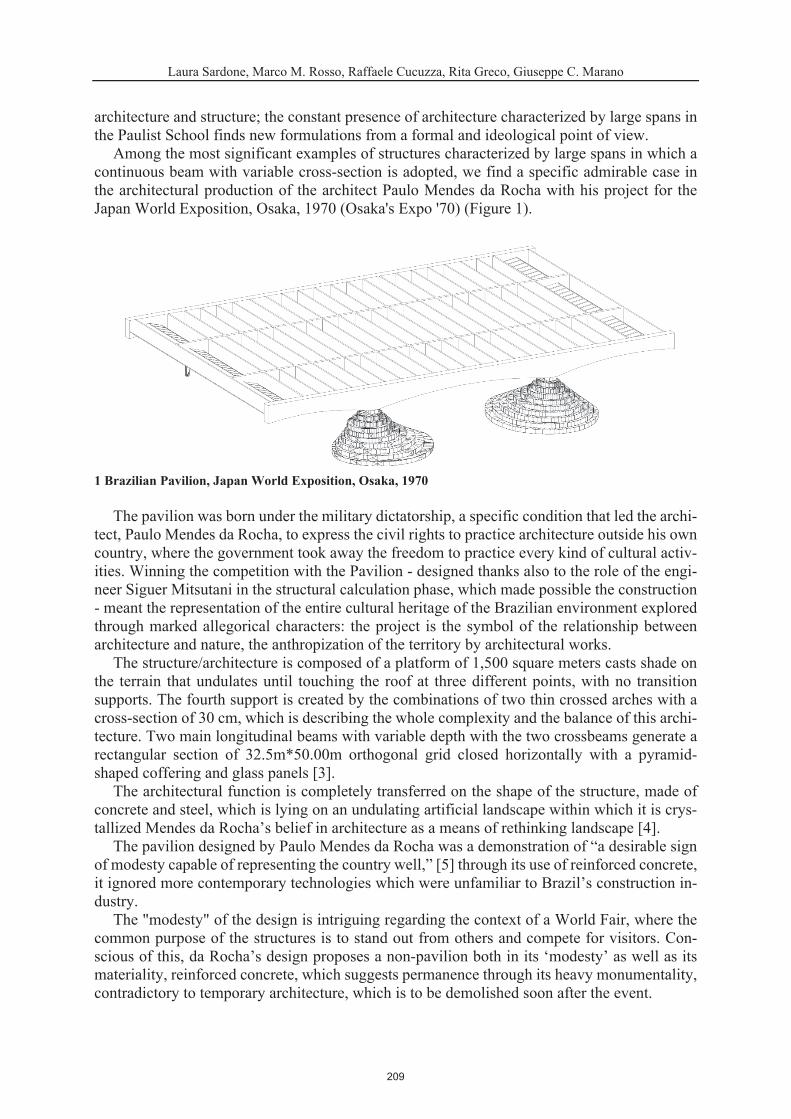
1 Brazilian Pavilion, Japan World Exposition, Osaka, 1970
209

2 Exploded view of the Brazilian Pavilion at the Osaka Expo, 1970. In red: main beams with variable cross-section.
210
2 COMPUTATIONAL GEOMETRY AND ANALYTICAL MODEL OF THE VARIABLE SECTION BEAM
3 Geometry of the main beam with non-constant section and reference axes
{ } , ,
+ + + + = 0
211
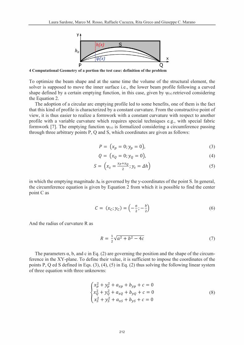
4 Computational Geometry of a portion the test case: definition of the problem
= = 0; = 0 ,
= = 0; = 0 ,
= = ; =
= ( ; ) = ;
= + 4
+ + + + = 0+ + + + = 0+ + + + = 0
212
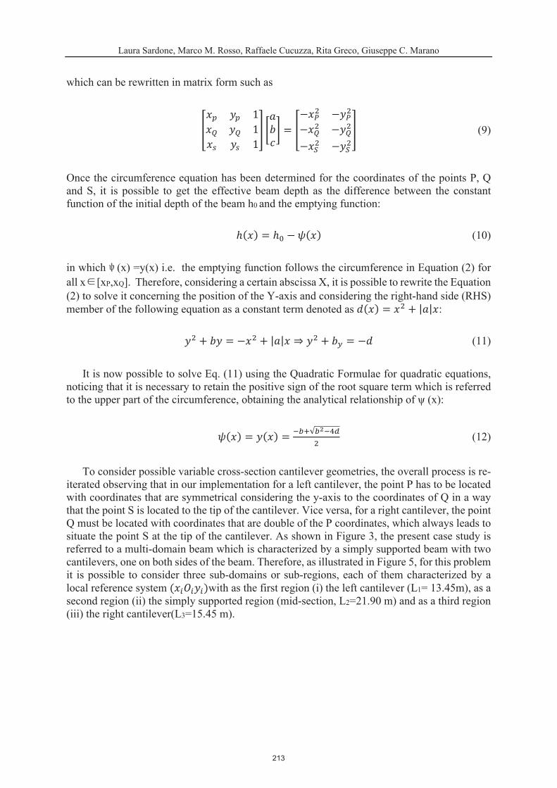
111
=
( ) = ( )
( ) = + | |
+ = + | | + =
( ) = ( ) =
( )
213

5 Multi-domain subdivision related to the case study problem.
( ) ( ) = ( )
( ) = ( )
( ) = ( )
( ) + + + = 0( ) + + + = 0
( ) + + + = 0
( ) =
( ) = ( )
( ) = [2( )( ) + ( ) ( )]
=
214

=( )
2.1 The Optimization Problem
{ }
= ,
= 2 arccos | |
= ( sin( ))
. . = = [ ]
3 NUMERICAL DEVELOPMENT THROUGH VISUAL PROGRAMMING
215
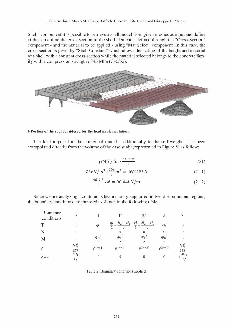
6 Portion of the roof considered for the load implementation.
45 55
25 / = 4612.5. = 90.44 /
2 2+
2 2 2 2
2 2
+
216

7 Application of boundary conditions; sections related to the Table 2.
{ } ,
= ,
217

4 NUMERICAL DEVELOPMENT AND OPTIMIZATION COMPARISON WITH MATLAB IMPLEMENTATION
( )( )( )( )( )( )
=
( )00
100
000
( ) 10000
0 00000
0 00000
( )( )( )( )( )( )
000( )( )( )
( ) = ( )( )
+ ( )( )
+( )
,
( ) = ( ) = ( ) ( )( )
,
( ) = ( ) = ( )( )
,
( ) = ( )( )
+ ( )( )
+( )
,
( ) = ( ) = ( )( )
,
( ) =( )
.
( ) ( ) ( )
bvp4c
218
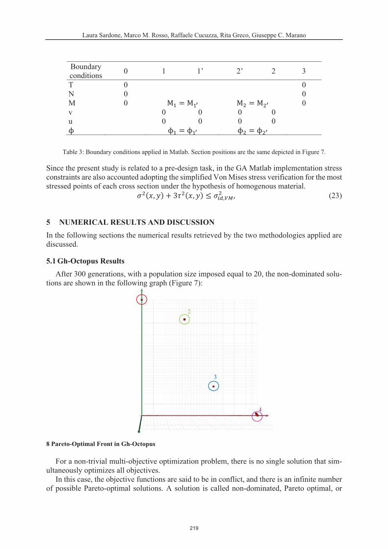
M = M M = M
= =
( , ) + 3 ( , ) , ,
5 NUMERICAL RESULTS AND DISCUSSION
5.1 Gh-Octopus Results
8 Pareto-Optimal Front in Gh-Octopus
219

9 Solution developed by Octopus Solver summarized in Table 3.
220

10 Shape Comparison between the main beam of Brazil's Pavilion (Expo Osaka, 1970) and the beam sub-jected to the Optimization process.
5.2 Matlab-ga results
11 Matlab-ga shape result and graphs
5.3 Results Discussion
221

REFERENCES
222

223
SOLVING PESSIMISTIC BILEVEL OPTIMIZATION PROBLEMSWITH EVOLUTIONARY ALGORITHMS
A PRELIMINARY STUDY
Margarita Antoniou1,2 and Gregor Papa1,2
1Jozef Stefan Institute,2Jozef Stefan International Postgraduate School
Ljubljana, Slovenia{name.surname}@ijs.si
Keywords: Pessimistic Bilevel Optimization, Nested Optimization, Evolutionary Algorithms
Abstract. It is common in practice, an optimal solution of a decision-maker to depend heavilyon the response of another decision-maker, formulating a bilevel optimization problem. The op-timization of a bilevel problem aims to achieve the optimum solution of the upper-level, takinginto consideration the optimal lower-level values too. When the lower-level problem is multi-modal, meaning that it has several global optima, an ambiguity about the optimal upper-levelsolution appears. The optimistic approach assumes that the follower will respond with an op-timal solution, that is favorable by the upper-level as well. In the pessimistic approach, theupper-level is optimising for the worst case. Various evolutionary algorithms have been imple-mented successfully to solve the optimistic approach of the bilevel problem. To the best of ourknowledge, these algorithms have not been extended to the pessimistic approach. In this paper,we use a multi-population nested Differential Evolution to solve the pessimistic bilevel problemwhen the lower-level has multiple global optima. The performance of the algorithm is examinedby solving a test-problem taken from the literature.
224

Margarita Antoniou and Gregor Papa
1 INTRODUCTION
The bilevel optimization problem is an optimization problem, operating as the upper-level,
that has another optimization problem as a constraint, at the lower-level. Bilevel problems
present many difficulties in its mathematical formulation, as they typically do not obey simplis-
tic properties such as convexity or continuity. Moreover, it is proven that even the simple case
of a linear bilevel optimization problem is NP-hard [1]. The bilevel optimization problem can
be also interpreted as a non-cooperative static Stackelberg game, as firstly introduced by von
Stackelberg in 1934 in the context of unbalanced economic markets [2].
When the lower-level problem is multimodal, meaning that it has several global optima, an
ambiguity about he optimal upper-level solution appears. The community has identified two
approaches to tackle this uncertainty, the optimistic and the pessimistic approach [3]. When
adopting an optimistic stance, the upper-level assumes that the lower-level will select the most
optimal solution that is also optimal for it. In the pessimistic approach, the upper-level is opti-
mising her objective making the worst-case assumptions about the decision of the lower-level.
The methods of solving the bilevel optimization problem can be divided into two main cate-
gories [3]. The first one refers to classical approaches, based on mathematical derivation meth-
ods, such as branch and bound [1], and is usually applied to well-behaved bilevel problems with
specific properties. The second one is based on hybrid and evolutionary approaches, which have
become more popular in the last years. Metaheuristic and evolutionary algorithms, in general,
do not need to make any assumptions about the objective functions of the problem and can
be applied to general bilevel problems [3]. Examples of this kind of Bilevel Evolutionary Al-
gorithms (BLEAs) are BlDE with Differential Evolution (DE) in both levels[4], NBLEA with
Genetic Algorithm in both levels[5], a memetic approach in [6], BLEAQ with genetic algorithm
and quadratic approximations [7], BL-CMA-ES with CMA-ES in both levels [8], etc. However,
all these evolutionary algorithms are adopting the optimistic approach for solving the BOP, as
it is easier to track.
While indeed the solution of the optimistic approach is much more tractable, it comes with
a drawback: the assumptions in the model, that a cooperation of the lower- with the upper-level
exists without any reward considered in her objective, are not realistic. On the contrary, the
pessimistic approach, while more conservative, can be interpreted as a bound and minimize
the risk of the worst case and give more robust solutions. Therefore, finding solutions for
the pessimistic case is of great importance in practice, when optimizing under uncertainty and
especially under worst-case scenario optimization.
The pessimistic approach is generally considered much more difficult to solve, and the solu-
tion methodologies made for the optimistic approach are not directly applicable to it. A survey
about the pessimistic bilevel optimization problem and its optimality conditions can be found
in [9, 10, 11]. There are several studies in the classical category, proposing solution methods
for pessimistic bilevel problems with specific mathematical properties, for example for the pes-
simistic bilevel linear problem [12], or a reduction method for the pessimistic quadratic-linear
bilevel[13]. From the hybrid and evolutionary approaches, the semivectorial pessimistic bilevel
problem has been approached with PSO [14] and Differential Evolution [15], with a multi-
objective problem in the lower-level. To the best of our knowledge, there is no Evolutionary
Algorithm studied to solve the general pessimistic bilevel optimization problem.
In this study, we aim to solve the pessimistic BOP by adopting EAs at both levels. The
algorithm has a nested structure. Therefore, for solving each upper-level candidate solution,
a lower-level optimization is conducted. The lower-level optimization algorithm has a multi-
225
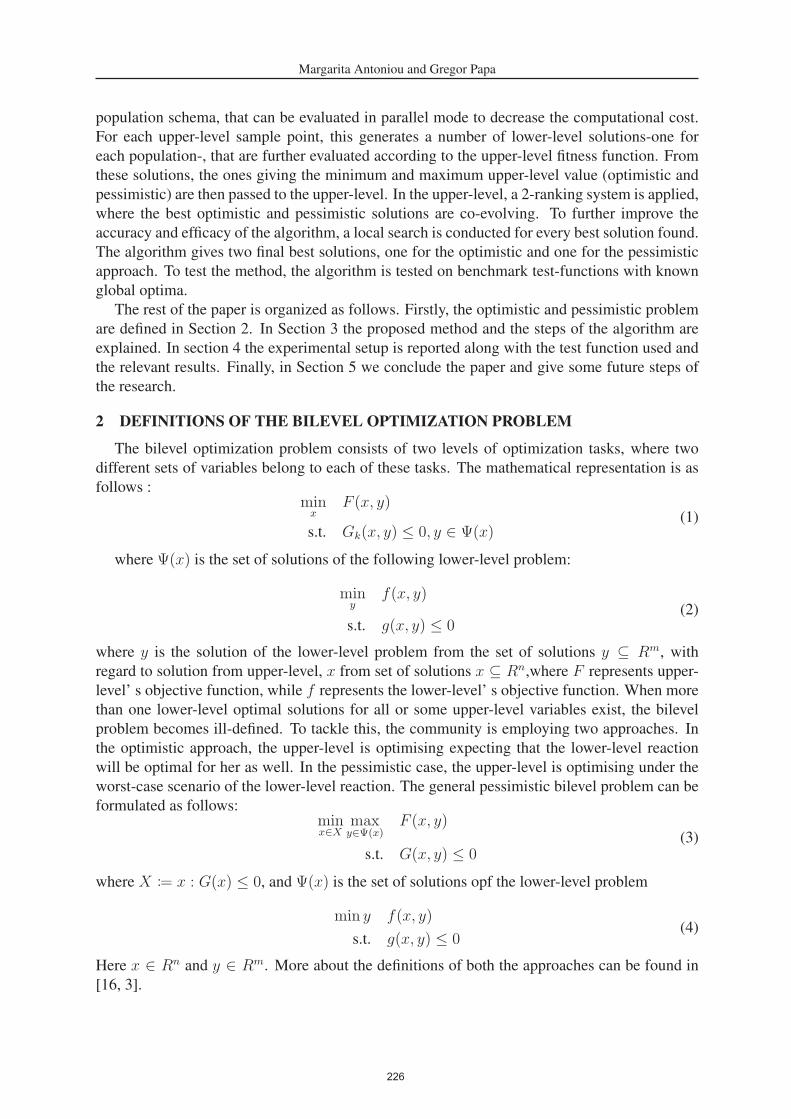
Margarita Antoniou and Gregor Papa
population schema, that can be evaluated in parallel mode to decrease the computational cost.
For each upper-level sample point, this generates a number of lower-level solutions-one for
each population-, that are further evaluated according to the upper-level fitness function. From
these solutions, the ones giving the minimum and maximum upper-level value (optimistic and
pessimistic) are then passed to the upper-level. In the upper-level, a 2-ranking system is applied,
where the best optimistic and pessimistic solutions are co-evolving. To further improve the
accuracy and efficacy of the algorithm, a local search is conducted for every best solution found.
The algorithm gives two final best solutions, one for the optimistic and one for the pessimistic
approach. To test the method, the algorithm is tested on benchmark test-functions with known
global optima.
The rest of the paper is organized as follows. Firstly, the optimistic and pessimistic problem
are defined in Section 2. In Section 3 the proposed method and the steps of the algorithm are
explained. In section 4 the experimental setup is reported along with the test function used and
the relevant results. Finally, in Section 5 we conclude the paper and give some future steps of
the research.
2 DEFINITIONS OF THE BILEVEL OPTIMIZATION PROBLEM
The bilevel optimization problem consists of two levels of optimization tasks, where two
different sets of variables belong to each of these tasks. The mathematical representation is as
follows :minx
F (x, y)
s.t. Gk(x, y) ≤ 0, y ∈ Ψ(x)(1)
where Ψ(x) is the set of solutions of the following lower-level problem:
miny
f(x, y)
s.t. g(x, y) ≤ 0(2)
where y is the solution of the lower-level problem from the set of solutions y ⊆ Rm, with
regard to solution from upper-level, x from set of solutions x ⊆ Rn,where F represents upper-
level’ s objective function, while f represents the lower-level’ s objective function. When more
than one lower-level optimal solutions for all or some upper-level variables exist, the bilevel
problem becomes ill-defined. To tackle this, the community is employing two approaches. In
the optimistic approach, the upper-level is optimising expecting that the lower-level reaction
will be optimal for her as well. In the pessimistic case, the upper-level is optimising under the
worst-case scenario of the lower-level reaction. The general pessimistic bilevel problem can be
formulated as follows:minx∈X
maxy∈Ψ(x)
F (x, y)
s.t. G(x, y) ≤ 0(3)
where X := x : G(x) ≤ 0, and Ψ(x) is the set of solutions opf the lower-level problem
min y f(x, y)
s.t. g(x, y) ≤ 0(4)
Here x ∈ Rn and y ∈ Rm. More about the definitions of both the approaches can be found in
[16, 3].
226
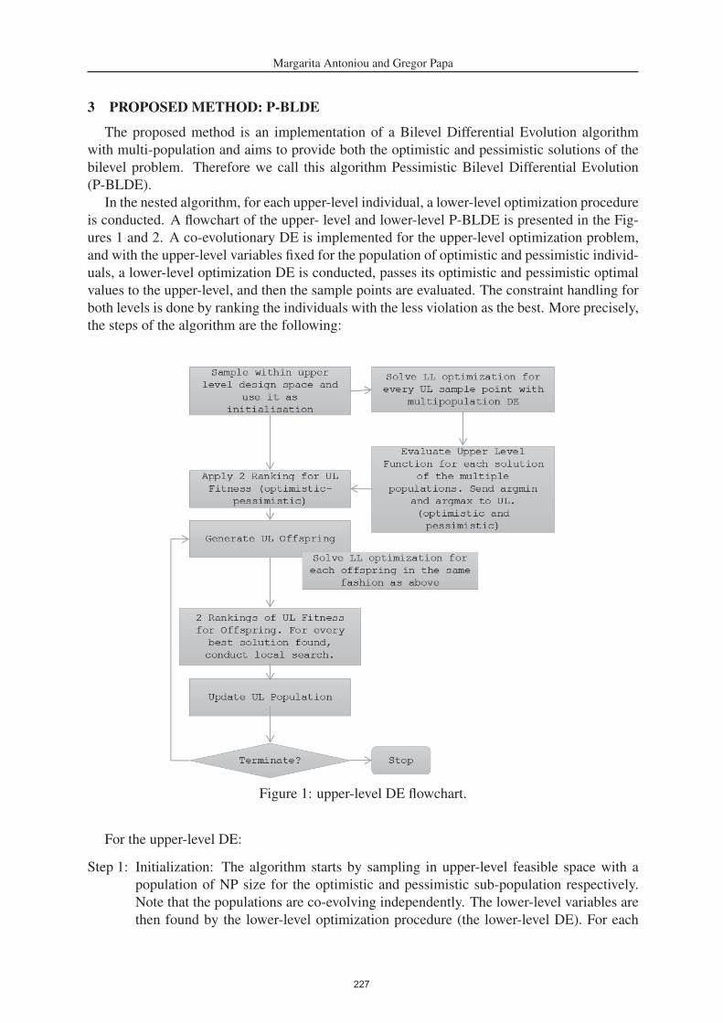
Margarita Antoniou and Gregor Papa
3 PROPOSED METHOD: P-BLDE
The proposed method is an implementation of a Bilevel Differential Evolution algorithm
with multi-population and aims to provide both the optimistic and pessimistic solutions of the
bilevel problem. Therefore we call this algorithm Pessimistic Bilevel Differential Evolution
(P-BLDE).
In the nested algorithm, for each upper-level individual, a lower-level optimization procedure
is conducted. A flowchart of the upper- level and lower-level P-BLDE is presented in the Fig-
ures 1 and 2. A co-evolutionary DE is implemented for the upper-level optimization problem,
and with the upper-level variables fixed for the population of optimistic and pessimistic individ-
uals, a lower-level optimization DE is conducted, passes its optimistic and pessimistic optimal
values to the upper-level, and then the sample points are evaluated. The constraint handling for
both levels is done by ranking the individuals with the less violation as the best. More precisely,
the steps of the algorithm are the following:
Figure 1: upper-level DE flowchart.
For the upper-level DE:
Step 1: Initialization: The algorithm starts by sampling in upper-level feasible space with a
population of NP size for the optimistic and pessimistic sub-population respectively.
Note that the populations are co-evolving independently. The lower-level variables are
then found by the lower-level optimization procedure (the lower-level DE). For each
227

Margarita Antoniou and Gregor Papa
individual, lower-level DE responds with an optimistic and a pessimistic solution that
is used to further evaluate the upper level.
Step 2: Upper-level mutation and recombination (crossover): The upper-level individuals of
each population are evolved with DE/rand/1/bin mutation strategy.
Step 3: Upper-level fitness evaluation: For each upper-level individual evolved, their fitness
is then evaluated. For this to happen, the lower-level optimal variables are needed.
Therefore, the lower-level optimization procedure is activated.
Step 4: Lower-level DE: for the fixed upper-level variables, a DE for lower-level is conducted,
including its initialization, evolution, and final lower-level optimistic and pessimistic
solutions.
Step 5: Upper-level termination: After the lower level is conducted, the upper-level fitness
is evaluated and then the termination criteria are checked. If they are satisfied, the
procedure stops and a final solution is given. Otherwise, the upper-level population is
Figure 2: lower-level DE flowchart.
228
Margarita Antoniou and Gregor Papa
updated with the best solution found so far and we go to step 2 again. The best solution
found for the pessimistic popupper levelation is further refined by local search (Interior
Point) using the fmincon of Matlab.
For the lower-level DE (Input: x vector from upper level):
Step 1: Initialization: The algorithm starts by sampling in a lower-level feasible space with
a population of NP size. The lower-level variables are then found by the lower-level
optimization procedure (the lower-level DE).
Step 2: Lower-level mutation and recombination (crossover): The optimistic lower-level indi-
viduals are evolved with DE/rand/1/bin, while the pessimistic population with DE/best/1/bin.
Step 3: Lower-level fitness evaluation: For each lower-level individual evolved, their fitness is
then evaluated in terms of both lower- and upper-level fitness function.
Step 4: Lower-level termination: After the lower-level is conducted, the lower-level fitness is
evaluated and then the termination criteria are checked. If they are satisfied, the pro-
cedure stops, and two final solutions are given. The minimum and maximum solutions
are labeled as optimistic or pessimistic respectively and passed to the upper-level. Oth-
erwise, the lower-level population is updated with the best solution found so far and we
go to step 2 again. For the optimistic population, the best solution found so far is the
one that is minimum for the lower-level function. For the pessimistic population, the
best solution found so far is the one that is minimum for the lower-level function and
maximum for the upper-level function.
The termination criteria are the maximum number of generations for both levels. The control
parameter values used are shown in Table 1. The population size refers to each sub-population
for both upper- and lower-level DE, while number of generations is for the whole procedure.
The parameter values were selected empirically, and no parameter tuning was conducted.
Table 1: Selected control parameters that are used in all of the reported results.
upper-level lower-level
Population size 10 30
Number of Generations 5 10
Crossover 0.9 0.9
Mutation uniformly(0.2,0.8) uniformly(0.2,0.8)
4 EXPERIMENTAL RESULTS
In this Section, we provide results for one test-problem, to illustrate the ability of the algo-
rithm to reach the optimistic and the pessimistic solutions of the problem. The test function
used is called mb 1 1 17, has multiple global minima in the lower-level, and is taken from
[11]. The optimistic problem has the following formulation:
minx,y∈Y (x)
x2 − y
s.t. x ∈ [0, 1], y ∈ [0, 3]
where Y (x) = arg minz∈[0,3]
[z − 1− x/10]2 − x/2− 1/2]2(5)
229

Margarita Antoniou and Gregor Papa
while pessimistic problem is as follows:
minx
maxy∈Y (x)
x2 − y
s.t. x ∈ [0, 1]
where Y (x) = arg minz∈[0,3]
{[z − 1− x/10]2 − x/2− 1/2]2}(6)
In Table 2 the known global optima for the optimistic and pessimistic approach of the problem
are reported. We also mention the pessimistic solution of the optimistic approach, which is
different than the global pessimistic solution.
Table 2: Known optima for the test function mb 1 1 17.
Solutions x y F
Optimistic 0.2106 1.799 -1.755
Optimistic-Pessimistic 0.2106 0.243 -0.1987
Pessimistic 0 0.2929 -0.2929
The test function has been independently run 30 times on an Intel(R) Core(TM) i7-7500
CPU @ 2.70GHz, 16 GB of RAM, and the Windows 10 operating system. The algorithm is
implemented in Matlab R2018b without any parallelization. In Table 3, the optimal values for
the optimistic and pessimistic solutions of the 30 runs of the P-BLDEA are reported. Also,
we report the min, median, and max of each solution and the runtime of the run in seconds.
We can see, that the solutions found for the optimistic approach, in general, reach the known
optimal solution with an accuracy of 0.0002 and for the pessimistic with 0.02. The runtime
is approximately 40 seconds per run. This relatively high number is justified if we take into
account that we are solving two problems at the same time (the optimistic and the pessimistic)
and given that the results are without any parallelization. Moreover, no parameter tuning or
adjustment of the population size is done for this experiment, while any tuning might lead to a
dramatic decrease in the runtime. In Figure 3 the upper- and lower-level 3D mesh and contour
plots are presented. Green dots are the known optimistic and pessimistic optima, while the red
stars show the median values of the optima found from P-BLDE. We can see that the algorithm
approximates the known solutions, managing to overcome the local optima of the lower-level
problem.
5 CONCLUSIONS AND FUTURE WORK
In this paper we proposed a nested EA to solve the pessimistic BOP. Firstly, we introduced
the topic and the motivation behind our research. Then, we gave the definitions of both the
optimistic and the pessimistic bilevel optimization problem. Next, the proposed method was
explained. The algorithm has a multi-population DE in each level, where an optimistic and pes-
simistic population co-evolve. The accuracy of the pessimistic lower-level solution is boosted
by a local search for every best solution found. The algorithm gives two final best solutions,
one for the optimistic and one for the pessimistic approach. The algorithm is tested in bench-
mark test-functions with known global optima, where it was shown to approximate well both
the optimistic and pessimistic known global optima.
Tuning of the parameters of the algorithm’s values, such as the population size and mutation
strategy to decrease the number of function evaluations and make the convergence faster is what
230

Margarita Antoniou and Gregor Papa
Table 3: Numerical results for P-BLDE for the 30 runs for test function mb 1 1 17.
Optimistic Pessimistic Runtime
Run F x y F x y (secs)
1 -1.7548 0.25883 1.8218 -0.23591 0.00064378 0.23591 41.5709
2 -1.7548 0.18484 1.7889 -0.28388 0.00064378 0.28388 40.7871
3 -1.7546 0.22197 1.8039 -0.28627 0.00064378 0.28627 39.6872
4 -1.7492 0.28308 1.8293 -0.27532 0.00054351 0.27532 38.7187
5 -1.7531 0.17097 1.7823 -0.23037 0.00064756 0.23037 39.1808
6 -1.7544 0.18277 1.7878 -0.29213 0.00064378 0.29213 38.2499
7 -1.7554 0.18815 1.7908 -0.2928 0.00064378 0.2928 42.3118
8 -1.7546 0.19378 1.7921 -0.29264 0.00064378 0.29264 37.9264
9 -1.7547 0.22099 1.8035 -0.25513 0.0006468 0.25513 42.5849
10 - 1.7526 0.1622 1.7789 -0.28134 0.00053724 0.28134 41.1649
11 -1.7553 0.1681 1.7835 -0.27213 0.00064378 0.27213 41.6821
12 -1.7546 0.18886 1.7903 -0.26977 0.00055272 0.26977 40.2938
13 -1.7538 0.2367 1.8098 -0.27128 0.00054427 0.27128 37.604
14 -1.7548 0.22897 1.8073 -0.29355 0.00064378 0.29355 37.5585
15 -1.7548 0.21446 1.8008 -0.2276 0.00054055 0.2276 37.7102
16 -1.7552 0.2127 1.8004 -0.27017 0.00053614 0.27017 37.4811
17 -1.755 0.22051 1.8037 -0.29301 0.00064378 0.29301 38.0905
18 -1.7561 0.19796 1.7952 -0.28992 0.00054281 0.28992 40.0531
19 -1.755 0.1998 1.7949 -0.1681 0.00053696 0.1681 48.6323
20 -1.7556 0.23253 1.8097 -0.28668 0.00053577 0.28668 46.1897
21 -1.7543 0.22525 1.805 -0.27192 0.00064378 0.27192 43.55
22 -1.7544 0.18446 1.7884 -0.20746 0.00064347 0.20746 49.4864
23 -1.7545 0.19986 1.7944 -0.28558 0.00064378 0.28558 51.1232
24 -1.7545 0.19628 1.7931 -0.29185 0.00064378 0.29185 51.7637
25 -1.7552 0.23102 1.8085 -0.28905 0.00064378 0.28905 57.5057
26 -1.7583 0.19052 1.7946 -0.20317 0.00064378 0.20317 62.2715
27 -1.7542 0.22883 1.8066 -0.23595 0.00053797 0.23595 51.1604
28 -1.7561 0.20439 1.7979 -0.2693 0.00054018 0.2693 49.5794
29 -1.7548 0.20328 1.7962 -0.26064 0.00054826 0.26064 50.1431
30 -1.7552 0.1851 1.7894 -0.29031 0.00053981 0.29031 53.1746
Min -1.7492 0.1622 1.7789 -0.29355 0.00053577 0.1681 37.481
Median -1.7548 0.20157 1.7957 -0.27372 0.00064378 0.27372 41.626
Max -1.7583 0.28308 1.8293 -0.1681 0.00064756 0.29355 62.272
we are working on at the moment. The immediate next step of this research is to take advantage
of the high parallelization of EAs, which will dramatically decrease the computational cost and
reach higher accuracy. Also, methods known to work well for reducing the computational cost
in the optimistic approach state-of-the-art methods, such as the use of surrogates and several
mappings between the upper- and the lower-level solutions, are under investigation. Moreover,
the strategy can work independently of the EA used, meaning that other evolutionary algorithms
more suitable for multimodal problems in the lower-level can be tested, and/or known BLEAs
from the literature can be implemented to find the optimistic solution.
231

Margarita Antoniou and Gregor Papa
00.2
0.40.6
0.81 0
2
−2
0
x
y
upper − level
−0.5
−0.5−0.5
−0.3
−0.3−0.3
0
00
−1
−1−1
−1.5
−1.5−1.5
−1.8
−1.8−1.8
−2
−2−2
0 0.2 0.4 0.6 0.8 10
0.5
1
1.5
2
2.5
3
x
y
upper − level
00.2
0.40.6
0.81 0
20
10
x
y
lower − level10
55
5 33
32.5
2.52.5
22
21.5
1.51.5
11
1
0.5
0.5
0.5
0.50.5
0.5
0.4
0.4
0.40.4
0.40.4
0.4
0.3
0.3
0.3
0.30.3
0.30.3
0.3
0 2
0.20.2
0.2
0.2
0.2
0.2
0.20.2
0.2
0.1
0.10.1 0.1
0.1
0.1
0.1
0.10.1
0.1
0.1 0.1
0.10.1 0.1
0.10.1
0.1
0.10.1
0.1
0 0.2 0.4 0.6 0.8 10
1
2
3
x
y
lower − level
Figure 3: Upper- and lower-level 3D mesh and contour plots. Green dots are the known opti-
mistic and pessimistic optima, while with red stars the median values of the optima found from
P-BLDE.
Acknowledgements
This work was supported by the Slovenian Research Agency (research core funding No. P2-
0098), by the European Union’s Horizon 2020 research and innovation programme under grant
agreement No. 692286 (SYNERGY), and under the Marie Skłodowska-Curie grant agreement
No. 722734 (UTOPIAE).
REFERENCES
[1] P. Hansen, B. Jaumard, and G. Savard, “New branch-and-bound rules for linear bilevel
programming,” SIAM Journal on scientific and Statistical Computing, vol. 13, no. 5, pp.
1194–1217, 1992.
[2] H. von Stackelberg, “Grundlagen der theoretischen volkswirtschaftslehre (translated as:
The theory of the market economy),” W. Hodge & Co. Ltd., London, 1952.
[3] A. Sinha, P. Malo, and K. Deb, “A review on bilevel optimization: from classical to evolu-
tionary approaches and applications,” IEEE Transactions on Evolutionary Computation,
vol. 22, no. 2, pp. 276–295, 2017.
232

Margarita Antoniou and Gregor Papa
[4] J. S. Angelo, E. Krempser, and H. J. Barbosa, “Differential evolution for bilevel program-
ming,” in 2013 IEEE Congress on Evolutionary Computation. IEEE, 2013, pp. 470–477.
[5] A. Sinha, P. Malo, and K. Deb, “Test problem construction for single-objective bilevel
optimization,” Evolutionary computation, vol. 22, no. 3, pp. 439–477, 2014.
[6] M. M. Islam, H. K. Singh, T. Ray, and A. Sinha, “An enhanced memetic algorithm for
single-objective bilevel optimization problems,” Evolutionary computation, vol. 25, no. 4,
pp. 607–642, 2017.
[7] A. Sinha, P. Malo, and K. Deb, “Evolutionary algorithm for bilevel optimization using
approximations of the lower level optimal solution mapping,” European Journal of Oper-ational Research, vol. 257, no. 2, pp. 395–411, 2017.
[8] X. He, Y. Zhou, and Z. Chen, “Evolutionary bilevel optimization based on covariance
matrix adaptation,” IEEE Transactions on Evolutionary Computation, vol. 23, no. 2, pp.
258–272, 2018.
[9] J. Liu, Y. Fan, Z. Chen, and Y. Zheng, “Pessimistic bilevel optimization: a survey,” In-ternational Journal of Computational Intelligence Systems, vol. 11, no. 1, pp. 725–736,
2018.
[10] S. Dempe, B. S. Mordukhovich, and A. B. Zemkoho, “Necessary optimality conditions in
pessimistic bilevel programming,” Optimization, vol. 63, no. 4, pp. 505–533, 2014.
[11] W. Wiesemann, A. Tsoukalas, P.-M. Kleniati, and B. Rustem, “Pessimistic bilevel opti-
mization,” SIAM Journal on Optimization, vol. 23, no. 1, pp. 353–380, 2013.
[12] S. Dempe, G. Luo, and S. Franke, Pessimistic bilevel linear optimization. Technische
Universitat Bergakademie Freiberg, Fakultat fur Mathematik und . . . , 2016.
[13] A. V. Malyshev and A. S. Strekalovsky, “Global search for pessimistic solution in bilevel
problems,” in Proceedings of the Toulouse global optimization workshop, 2010, pp. 77–80.
[14] M. J. Alves, C. H. Antunes, and P. Carrasqueira, “A pso approach to semivectorial bilevel
programming: pessimistic, optimistic and deceiving solutions,” in Proceedings of the 2015Annual Conference on Genetic and Evolutionary Computation, 2015, pp. 599–606.
[15] M. J. Alves and C. H. Antunes, “A differential evolution algorithm to semivectorial bilevel
problems,” in International Workshop on Machine Learning, Optimization, and Big Data.
Springer, 2017, pp. 172–185.
[16] J. Liu, Y. Fan, Z. Chen, and Y. Zheng, “Methods for pessimistic bilevel optimization,” in
Bilevel Optimization. Springer, 2020, pp. 403–420.
233

THE HYBRID GLOBAL OPTIMIZATION ALGORITHM ON THE BASIS OF A FIREWORKS ALGORITHM
P. Paździor , M. Szczepanik
Abstract
The article shows the composition of the developed hybrid optimization algorithm, as well as the method and results of testing operation. The new algorithm was inspired by the Fireworks Algorithm and the general principle of operation of Evolutionary Algorithms. The goal of de-veloping a new computational solution was to minimize the number of necessary calls to the objective function to reach the global minimum with the desired accuracy. The correspondingcases compared the results obtained for various test functions of two or more variables.
Keywords:
234
1 INTRODUCTION
2 ALGORITHM
2.1 Evolutionary and Fireworks Algorithms
235

2.2 The hybrid global optimization algorithm
236

237
2.3 Steering parameters
238

3 TESTING FUNCTIONS
3.1 Parabolic function
3.2 Step function
239

3.3 Beale's function
3.4 Rastrigin function
240

3.5 Easom function
241

242

4 RESULTS
EA FWA Hybrid
4976
5706
12801 13560 10370
13228 13161 8184
9990
5 CONCLUSIONS
243

6 ACKNOWLEDGEMENT
REFERENCES
Computational Optimization Methods
SCIENCE
Student Scientific Conference „Computer Methods – 2020”
Computer Science
SPACE
Bulletin of the Instituteof Automation and Robotics WAT
New Computing Techniques in Physics Research II
Evolutionary Computation, IEEE Transactions
244

BRIDGES MONITORING: AN APPLICATION OF AI WITH GAUSSIAN PROCESSES
Rebecca Asso1, Raffaele Cucuzza2, Marco M. Rosso2, Davide Masera1 and Giuseppe C. Marano2
Abstract.
Keywords:
245

1 INTRODUCTION
246

2 STATE OF THE ART
2.1 Bearings of bridges monitoring
247

248

2.2 Gaussian Processes
249

3 CASE STUDY: THE BRIDGE
250

4 DATA ANALYSIS
251

4.1 Preprocessing
4.2 Postprocessing
K
252
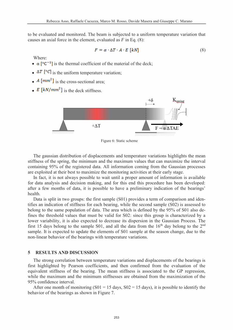
F
5 RESULTS AND DISCUSSION
253
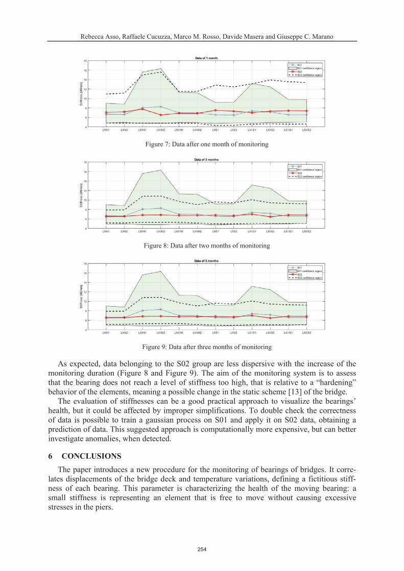
6 CONCLUSIONS
254

7 APPENDIX
Figure 12: Gaussian Regression of LXN1 and LXN2 after one month of data
255

Figure 12: Gaussian Regression of LXN1 and LXN2 after two months of data
Figure 12: Gaussian Regression of LXN1 and LXN2 after three months of data
256

Figure 12: Gaussian Regression of LXIIN1 and LXIIN2 after one month of data
Figure 12: Gaussian Regression of LXIIN1 and LXIIN2 after two months of data
257
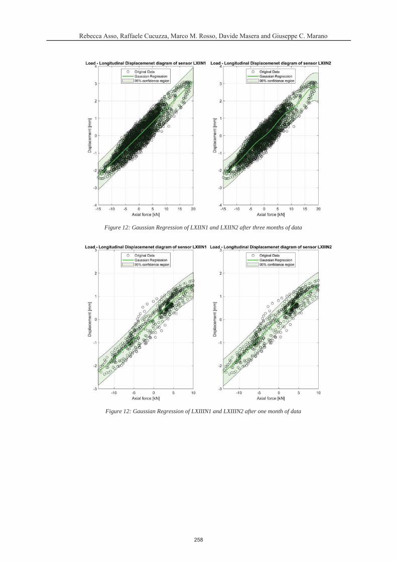
Figure 12: Gaussian Regression of LXIIN1 and LXIIN2 after three months of data
Figure 12: Gaussian Regression of LXIIIN1 and LXIIIN2 after one month of data
258

Figure 12: Gaussian Regression of LXIIIN1 and LXIIIN2 after two months of data
Figure 12: Gaussian Regression of LXIIIN1 and LXIIIN2 after three months of data
8 ETHICS DECLARATION
259

REFERENCES
J. Struct. Eng.
Philos. Trans.
R. Soc. A Math. Phys. Eng. Sci.
Vibration-Based Techniques for Damage Detection and Localization in Engineering Structures
J. Perform. Constr.
Facil.
Struct.
Infrastruct. Eng.
J. Civ. Struct. Heal. Monit.
J. Civ. Struct. Heal. Monit.
260
Lect. Notes Comput. Sci.
(including Subser. Lect. Notes Artif. Intell. Lect. Notes Bioinformatics)
Big Data Anal.
Struct. Heal.
Monit.
261

SOFTWARE PACKAGE FOR THE NUMERICAL SOLUTION OF NONLOCAL OPTIMIZATION PROBLEMS
Pavel S. Sorokovikov , and Alexander Yu. Gornov
Abstract
The paper discusses the developed first version of the MEOPT (“Multi-Extremal OPTimization”) software package designed to solve multiextremal problems of parametric identification of nonlinear models. The project includes the following components: software framework that provides a uniform approach to the implementation of algorithms and includes basic functionality; libraries of optimization algorithms; collection of test problems with known solutions; tool and service modules; metacomponents. The implemented libraries of optimization algorithms include multidimensional nonconvex optimization methods and algorithms for solving auxiliary problems of global univariate search. The library of test problems includes both mathematical programming problems and tasks of optimization of dynamic systems. The software package was developed using the C language and the GCC compiler; it operates under Linux, Windows, and Mac OS operating systems. To date, prototypes of the main modules of the package have been completed. The technical testing of the first version of the software was carried out.
Keywords:
262

1 INTRODUCTION
263

2 FORMULATION OF THE PROBLEM
2.1 Mathematical statement
x f x t u t t x t x
t t t nx t x t x t x t
ru t u t u t u t
f x t u t t
t u tt U
rl gU u t R u u t u
rl gu u R
u t
I u x t
j jI u x t j m
j jI u g x t u t t j m mt
j x t j m jg x t u t t j m mt
264

un
ut ih i n t un
2.2 Technological statement
3 LOGICAL STRUCTURE OF THE SOFTWARE PACKAGE
265

4 IMPLEMENTED FUNCTIONAL SUBSYSTEMS
266

5 OPERATING MODES OF THE SOFTWARE PACKAGE
5.1 Available operating modes
267
5.2. Probabilistic single-level dynamic computation scheduler for the global search
k kf fk k
recf f f krecf k
f i
i Mf f M
k
k
k
6 CONCLUSIONS
268

7 FUNDING
REFERENCES The set of programs for the approximate solution of
optimal control problems (application description)
DIOSdialogue complex. Section of nonlinear programming
Solution of optimal control problems in system DIOS
Application software packages: experience of use
Algorithms and programs:Information Bulletin 2(71)
Application softwarepackages. Development experience
Approximate methods of optimal control
Izvestia of the Academy of Sciences of the USSR. Technicalcybernetics, 4
OPTCON software package for solving optimal controlproblems. User’s manual
18th Baikal All-Russian Conference “Information and MathematicalTechnologies in Science and Management”. Part 3
Practical methods for optimal control and estimation using nonlinearprogramming
A unified computational approach to optimal controlproblems
User’s guide for DIRCOL: A direct collocation method for the numericalsolution of optimal control problems, Vol. II
MINOPT: A software package for mixed-integernonlinear optimization
User’s guide OC-ODE (version 1.4). Technical report
269

BMC Bioinformatics 10
MUSCOD-II User’s Manual
Mathematical ProgrammingComputation 11
TomlabOptimization Inc. 260
Imperial college London optimal control softwareuser guide (ICLOCS), Vol. 28
2010IEEE International Symposium on Computer-Aided Control System Design
Optimization and optimal control inautomotive systems 1
Computational technologies for solving optimal control problems
Bulletin of the Buryat State University. Mathematics, computerscience 4
Proceedings of the 6th International Workshop “Critical Infrastructures: Contingency Management, Intelligent, Agent-Based, Cloud Computing and Cyber Security” (IWCI 2019) 169
18th InternationalConference on Mathematical Optimization Theory and Operations Research (MOTOR 2019)
IOPConference Series: Materials Science and Engineering 1047
63rd All-Russian Scientific Conference of MIPT. Applied Mathematics and Computer Science
270

TESTS OF SCRATCH RESISTANCE OF POLYMER MATERIAL SURFACES
Janusz W. Sikora and Daniel Pieniak
Abstract
The paper presents the results of comparative tests of resistance to scratching of two polymersamples made via the extrusion method. The first sample was a homogenous low-density poly-ethylene Lupolen 2426 H, while the second sample was a two-layer polymer of the same thick-ness with an outer layer of polypropylene Marlex HGX-030SP and an inner layer of Lupolen2426 H. The Micro Scratch Tester and the Dektak 150 profilometer were used to perform the appropriate measurements. The following values were recorded: coefficient of friction, force of friction, depth of indenter penetration and residual depth after scratching. Surface profilo-grams and boxwhisker diagrams of hardness, width of the gap and area of the crack cross-section were made. The results of the research indicate the possibility of applying polypropyl-ene to a layer protecting low-density polyethylene against mechanical damage, especiallyagainst scratches.
Keywords:
271

1 INTRODUCTION
2 TEST CHARACTERISTICS
2.1 Test object
272

2.2 Test method
273

274

3 TEST RESULTS
3.1 Results of measurements on the MST scratch tester
275
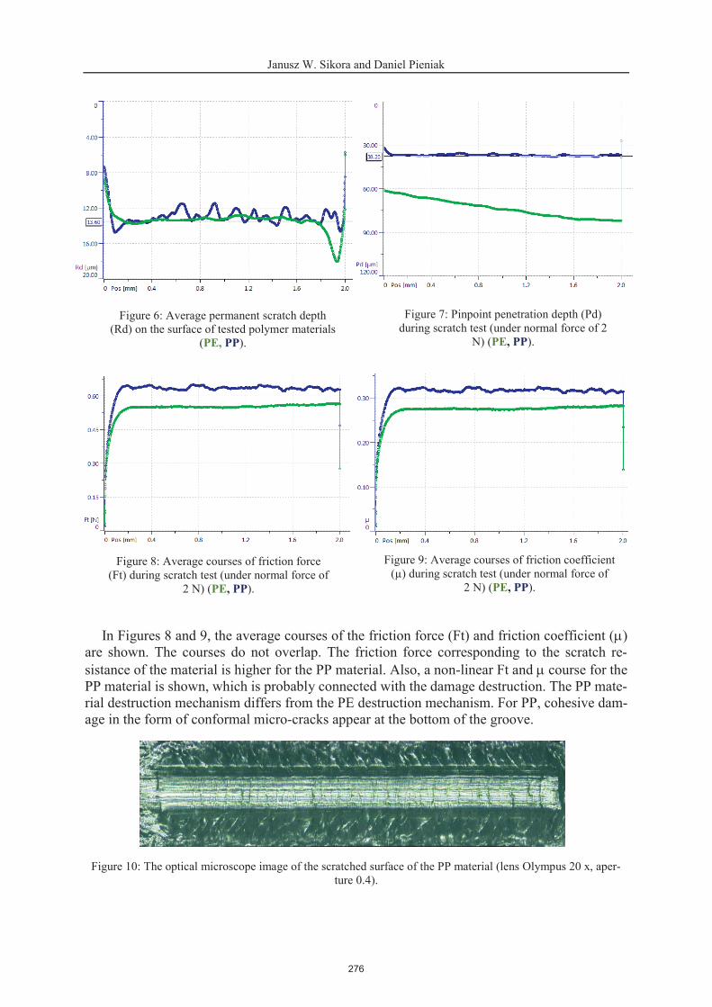
PE, PP PE, PP
PE, PPPE, PP
276
3.2 Results of tests on the Dektak 150 profilometer
277

4 CONCLUSIONS
REFERENCES
Polymers for Advances Technologies, 27
Scratch behavior of polymeric materials 2nd Edition
Scratch damage resistance of silica-based sol–gel coatings on polymeric substrates. 2nd Edition
Journal of Reinforced Plas-tics and Composites 29
Inżynieria Maszyn, 18
278

Measurement of mechanicalproperties 5
Dental Materials 29
Applied Surface Science, 256
Tribology International 44
Materials Science and Engineering: A, 364
Progress inOrganic Coatings 48
‐Macromoleculars Materials and Engineering 287
AppliedComposite Materials, 6,
Polymer Engineering and Science, 36
279

Institute of Structural Analysis and Antiseismic Research
National Technical University of Athens, Greece
EUROGEN 2021
Proceedings of the 14th International Conference on Evolutionary and Deterministic Methods For Design, Optimization and Control N. Gauger, K. Giannakoglou, M. Papadrakakis, J. Periaux (Eds.)
First Edition, September 2021
ISBN: 978-618-85072-7-2