European Economic Review 119 (2019) 526–547

Contents lists available at ScienceDirect

European Economic Review

journal homepage: www.elsevier.com/locate/euroecorev

Targeted carbon tax reforms

�

Maia King

a , Bassel Tarbush

b , ∗, Alexander Teytelboym

c

a Blavatnik School of Government and Nuffield College, University of Oxford, United Kingdom

b Merton College, University of Oxford, United Kingdom

c Department of Economics, St. Catherine’s College and the Institute for New Economic Thinking at the Oxford Martin School, University

of Oxford, United Kingdom

a r t i c l e i n f o

Article history:

Received 19 January 2018

Accepted 1 August 2019

Available online 9 August 2019

JEL classification:

D51

D62

H23

Q54

Keywords:

Emissions tax

Carbon tax

Pollution tax

Climate change

Environmental tax reform

Input-output linkages

Intersectoral network

a b s t r a c t

In the presence of intersectoral linkages, sector-specific carbon tax changes can have com-

plex general equilibrium effects. In particular, a carbon tax on the emissions of a sector can

lead to an increase in aggregate emissions. We analytically characterise how incremental

taxes on the emissions of any set of sectors affect aggregate emissions. We show that car-

bon tax reforms that target sectors based on their position in the production network can

achieve a greater reduction in aggregate emissions than reforms that target sectors based

on their direct emissions alone. We illustrate the effects of carbon tax reforms by calibrat-

ing our intersectoral network model to the economies of two countries.

© 2019 Elsevier B.V. All rights reserved.

1. Introduction

To have a reasonable chance of avoiding the dangerous effects of climate change, cumulative anthropogenic carbon emis-

sions must be limited to one trillion tonnes ( Allen et al., 2009; Meinshausen et al., 2009 ). Achieving this target requires

coordinated global action and a substantial increase in the price of carbon ( High-Level Commission on Carbon Prices, 2017 ).

However, current carbon pricing policies around the world are piecemeal and are imposed only on certain sectors ( World

Bank and Ecofys, 2018 ). In this paper, we analyse the effects of incremental (or marginal) sector-specific carbon tax changes,

which we refer to as carbon tax reforms . In the presence of intersectoral linkages, such reforms can have complex general

equilibrium effects on aggregate emissions.

� We would like to thank Daron Acemoglu, David Baqaee, Ozan Candogan, Justin Caron, Emanuele Ciola, Luís Fonseca, Cameron Hepburn, Ernest Liu, Linus

Mattauch, Adrian Odenweller, Rick van der Ploeg, two anonymous referees, and participants at the 2018 Symposium on Social and Economic Networks

(Monash Business School) and at the 2018 EEA-ESEM Congress for their comments. Teytelboym is grateful for the support of the Oxford Martin Programme

on the Post-Carbon Transition. ∗ Corresponding author.

E-mail addresses: maia.king@bsg.ox.ac.uk (M. King), bassel.tarbush@economics.ox.ac.uk (B. Tarbush), alexander.teytelboym@economics.ox.ac.uk

(A. Teytelboym).

https://doi.org/10.1016/j.euroecorev.2019.08.001

0014-2921/© 2019 Elsevier B.V. All rights reserved.

M. King, B. Tarbush and A. Teytelboym / European Economic Review 119 (2019) 526–547 527

We analyse the effects of carbon tax reforms in an intersectoral input–output network in which firms trade intermediate

inputs and sell their goods to a representative consumer. A sector’s use of different intermediate inputs produces emissions

directly and indirectly. For example, a factory might use coal, electricity, and labour. For every unit of coal that it uses, the

factory produces emissions directly. But when the factory uses electricity, it does not produce emissions directly; rather the

utility company that supplies the factory is likely to produce emissions in the process of electricity generation. Therefore, by

using electricity the factory also produces emissions indirectly. The impact of taxing the emissions of a sector on aggregate

emissions will therefore be determined by all the intersectoral linkages.

We assume that the government can only implement incremental sector-specific carbon taxes. The main contribution of

our paper is to track the propagation of the effects of such taxes throughout the economy. Our analysis focuses on marginal

tax changes and ignores damages resulting from emissions. 1

Our main result characterises the effects of carbon tax reforms in the presence of intersectoral linkages. We show that

the effect of any multi-sector carbon tax reform can be linearly decomposed into the aggregate emissions impacts of the

taxed sectors. The aggregate emissions impact of a sector is the change—which can be positive or negative—in aggregate

emissions that results from incrementally taxing the emissions of that sector alone. We refer to sectors with negative ag-

gregate emissions impacts as key sectors . Therefore, a policymaker, who is interested in emissions reduction but is (politi-

cally or technologically) constrained to incrementally taxing the emissions of only certain sectors, targets key sectors with

the greatest aggregate emissions impacts (in absolute value). The carbon tax reform that delivers the greatest reduction

in aggregate emissions—the most effective carbon tax reform—imposes a carbon tax on a sector if and only if it is a key

sector.

A sectoral carbon tax affects aggregate emissions in three ways. First, a taxed sector’s production mix switches from

more polluting to less polluting direct inputs. The fall in the sector’s input demands reduces the output and emissions of

all direct and indirect suppliers to the sector. Second, the taxed sector’s output price rises which causes its buyers to switch

away from using the sector’s good as an input and reduces the output and emissions of all its direct and indirect buyers.

The magnitudes of these upstream and downstream influences of a sector are a function of the sector’s position within the

intersectoral production network. Third, the tax revenue is rebated to the consumer who is therefore able to consume more

from every sector. This tax rebate effect (or aggregate demand channel) increases sectoral output and aggregate emissions.

Whether taxing the emissions of a sector has a positive or negative impact on aggregate emissions depends on (i) the

tax rebate effect, (ii) the sector’s intersectoral influence on emissions, and (iii) the sector’s level of emissions relative to

aggregate emissions. If the sector’s emissions are sufficiently high, the sector will always be a key sector. But even sectors

with low emissions might have high intersectoral influence on emissions in the intersectoral network, and could therefore

be key sectors. However, if the sector’s emissions are low, then the tax rebate effect can exceed the other effects, netting a

positive effect on aggregate emissions following a sectoral carbon tax.

We calibrate our model to the economies of the United States and Pakistan and estimate the aggregate emissions im-

pacts of each industrial sector. For Pakistan’s economy, we find that while the non-metallic minerals sector (e.g., cement)

emits approximately three times less carbon than the electricity production sector, taxing the emissions of the non-metallic

minerals sector would result in a greater fall in aggregate emissions than taxing the emissions of the electricity sector. The

fact that the non-metallic minerals sector has a greater aggregate emissions impact (in absolute value) than the electricity

sector is a result of the centrality of the non-metallic minerals sector in the intersectoral network. Moreover, taxing the

emissions of the non-metallic minerals and electricity sectors alone would deliver most of the emissions reduction from the

most effective carbon tax reform.

Our paper connects two strands of the literature: intersectoral input–output networks and environmental tax reforms.

The first strand is a rapidly growing literature that looks at the propagation of shocks in an interconnected economy. In the

zero-tax benchmark, our general equilibrium model is a static version of Long Jr. and Plosser’s (1983) real business cycles

model which is analysed by Acemoglu et al. (2012) . In this paper, we analyse the effects of adding emissions and emissions

taxes to that model. Sectors produce emissions according to an emissions function which is assumed to have constant

returns to scale in the inputs to production and we place no restrictions on the structure of the input–output network. We

therefore generalise the insights of Baylis et al. (2013, 2014) who pointed out that carbon taxes in some sectors can lead to

emissions reductions in other sectors thereby causing “negative leakage”. 2 , 3 The upstream and downstream effects of carbon

tax reforms in our model are similar to the structure of technology shock propagation in other models ( Shea, 2002; Baqaee,

1 In contrast, the analysis of optimal, non-marginal carbon taxes would require the policy-maker either to know the damages from emissions or to

specify an emissions reduction target. The calculation of optimal carbon taxes is usually done with sophisticated Integrated Assessment Models (IAMs) that

combine a {multi-sectoral, multi-regional, dynamic, stochastic, computable} general equilibrium model of the economy and an earth science model ( Metz

et al., 2001 ). These models are broadly of two types. Policy evaluation IAMs, such as GCAM, IMAGE, and MESSAGE, used by the Intergovernmental Panel

on Climate Change, calculate the most cost-effective paths to a fixed emissions target (e.g., net zero carbon emissions by 2050). Policy optimisation IAMs,

such as DICE/RICE, PAGE, and FUND additionally include a damage function (that maps emissions to the effects on output and consumption) which allows

them to calculate the socially optimal level of cumulative emissions. 2 The possibility of an overall positive effect on aggregate emissions resulting from sectoral taxes in our model is different from the channels described

in carbon leakage (i.e., offshoring of production due to domestic emission pricing; see, for example, Babiker, 2005 ). The tax rebate to the consumer is

central to our results, but it plays little role in carbon leakage. 3 Jarke and Perino (2017) discuss negative leakage in the context of incomplete cap-and-trade schemes.

528 M. King, B. Tarbush and A. Teytelboym / European Economic Review 119 (2019) 526–547

2015; Huremovic and Vega-Redondo, 2016 ). 4 In an important contribution, Baqaee (2016) showed that in the presence of

intersectoral linkages fiscal policy could be targeted at certain sectors in order to maximise impact on employment and

output; our results have a similar flavour. Our set-up is also related to models used in the input–output analysis of carbon

content of consumption and production (e.g., Turner et al., 2007; Wiedmann et al., 20 07; Wiedmann, 20 09; Davis and

Caldeira, 2010; Caron et al., 2017 ).

The second strand is a rich literature on environmental tax reforms. This work stems from the classic public economics

literature on tax reforms ( Buchanan, 1976; Feldstein, 1976; Guesnerie, 1977; Weymark, 1981 ). 5 One of the key questions in

the environmental tax reforms literature is whether the shift of the tax burden away from employment and income towards

consumer-harming pollution makes the consumer better off ( Copeland, 1994; Bovenberg and De Mooij, 1994; Bovenberg

and van der Ploeg, 1994; Bovenberg and Goulder, 1996; Bovenberg and van der Ploeg, 1996 ). 6 In contrast, in our model,

emissions do not affect utility directly i.e., emissions are not an externality. In the absence of externalities or other distor-

tions, optimal carbon taxes are zero in our benchmark economy. To motivate the reason for government intervention, we

imagine that the government simply has an exogenous reason to reduce carbon emissions (e.g., adhering to the Nationally

Determined Contribution as part of the Paris Agreement) and is constrained to implementing incremental sector-specific

carbon taxes. Moreover, we assume that all the tax revenue is rebated in full to the consumer and that the economy has

no unemployment or distortions (such as income or commodity taxes) prior to the introduction of a carbon tax reform.

However, we expect that the crux of our analysis would go through even in an economy with preexisting distortions ( Drèze

and Stern, 1987; 1990 ).

This paper is organised as follows. Section 2 introduces the model. Section 3 provides the benchmark solution in the

absence of emissions taxation. Section 4 considers the effect of carbon tax reforms on sectoral consumption, labour demand,

intermediate input use, output, and emissions. Section 5 introduces aggregate emissions impacts, identifies the key sectors,

and characterises the most effective carbon tax reform. Section 6 presents our calibration results. Section 7 concludes. The

Appendix provides the proofs and further details of the calibration.

2. Model

2.1. Sectors

Our model and notation build directly on Acemoglu et al. (2012) . Each of n competitive sectors produces a distinct good.

Sector i produces output Y i according to the Cobb–Douglas production function

Y i = l 1 −αi

n ∏

j=1

x αw i j

i j , (2.1)

where w i j ≥ 0 is the share of expenditure on input j in sector i ’s expenditure on intermediate inputs, α ∈ (0, 1) is the share

of intermediate goods in production, x ij is the input demand of sector i for the good produced by sector j , and l i is sector

i ’s demand for labour. 7 The matrix W = [ w i j ] is the economy’s input–output matrix. We assume that ∑ n

j=1 w i j = 1 for all i

which ensures constant returns to scale in production.

The emissions of sector i are determined by a constant returns to scale emissions function E i (x i 1 , . . . , x in ) that is increas-

ing (and differentiable) in intermediate inputs. 8 Sectoral emissions are a function of inputs directly rather than a function

of sectoral output. Therefore, depending on its input mix, a sector can produce the same level of output at different levels

of emissions.

The profit of (a representative firm in) sector i is given by

πi = p i Y i −n ∑

j=1

p j x i j − ωl i − λi tωE i , (2.2)

where ω is the competitive wage rate and t is the tax rate on emissions. We anchor the value of the tax to the wage so t ωis a per-unit tax on emissions. Here, λi ∈ {0, 1} is a parameter such that sector i taxed if and only if λi = 1 . By selecting an

appropriate vector λ∈ {0, 1} n we can analyse the effects of emissions taxes on any set of sectors.

4 Since taxes introduce non-linearities into our model, we solve our model using the first-order approach suggested by Acemoglu et al. (2015) . 5 See Myles (1995 , Chapter 6) for a summary. In this spirit, Allouch (2017) and Allouch and King (2018) examine the social welfare impacts of small and

incremental budget-balanced transfers in networks with private provision of local public goods. Galeotti et al. (2018) analyse targeting policies in networks

in which a planner has a budget to affect the marginal benefits of agents’ actions. 6 See Bovenberg and Goulder (2002 , Section 3) for a summary. 7 Since our focus is not on total factor productivity shocks, we normalise the usual TFP parameter to 1. 8 We will take the second-order conditions of the profit maximisation problem to be satisfied e.g., when E i is linear.

M. King, B. Tarbush and A. Teytelboym / European Economic Review 119 (2019) 526–547 529

i j kwji wkj

vik

wki

Fig. 3.1. Thin arrow i w ki −→ k represents how much of sector k ’s production depends directly on good i . Thick arrow i

v ik −→ k represents how much sector k ’s

production depends directly and indirectly (via j ) on good i .

2.2. Consumer

A representative consumer inelastically supplies one unit of labour ( l = 1 ) that can be hired by the sectors, and has

Cobb-Douglas preferences over consumption with utility function

U(C 1 , . . . , C n ) =

n ∏

i =1

C 1 /n i

. (2.3)

The utility function does not depend on the level of emissions. Emissions are not an externality in our model but rather

act as a friction on the production side in the presence of emissions taxes. We take the government’s reasons to reduce

emissions as exogenously given and we are not attempting to estimate the socially optimal level of emissions.

We assume perfect mobility of labour across sectors so there is a unique competitive wage ω. The government redis-

tributes the emissions tax revenue in full to the consumer. Therefore, the consumer’s budget constraint is given by

n ∑

i =1

p i C i ≤ ωl + T = ω + T , (2.4)

where T = tω

∑ n i =1 λi E i is the total emissions tax revenue. There are no profits from sector ownership due to the constant

returns to scale exhibited by production and emissions.

3. Zero-tax benchmark

When the emissions tax is zero, our economy essentially coincides with the economy presented in Acemoglu et al. (2012) .

Definition 1. A competitive equilibrium consists of prices p 1 , . . . , p n , a wage ω, consumption levels C 1 , . . . , C n , labour de-

mands l 1 , . . . , l n , and intermediate input quantities x ij for all i , j , such that (i) the consumer maximises her utility subject to

her budget constraint, (ii) the sectors maximise their profits, (iii) the markets for each good and labour clear, that is,

n ∑

i =1

l i = l = 1 , (3.1)

and, for each i ,

Y i = C i +

n ∑

j=1

x ji . (3.2)

In order to characterise the competitive equilibrium, we will employ standard definitions from the input–output literature

( Leontief, 1966 ).

Definition 2. The matrix V = [ v i j ] = (I − αW

′ ) −1 is the economy’s Leontief inverse . 9

We can alternatively write the Leontief inverse as

V = I + α(W

′ ) + α2 (W

′ ) 2 + . . . (3.3)

The ik element of the matrix W

′ , w ki , measures how much of sector k ’s production depends directly on the use of the

good produced by sector i . In Fig. 3.1 we represent this dependence as a thin arrow going from i to k (only links with positive

weight are shown). The ik element of the matrix ( W

′ ) 2 aggregates all weighted walks of length two going from i to k : it

measures how reliant k ’s production is on the use of good i through its use of the intermediate input j . In the network shown

in Fig. 3.1 , the ik element of ( W

′ ) 2 is equal to the product w k j w ji . Similar reasoning applies to the elements of ( W

′ ) h for h > 2.

9 V is well-defined because α ∈ (0, 1) and W is row-stochastic. Acemoglu et al. (2015) refer to the transposed matrix V ′ as the Leontief matrix .

530 M. King, B. Tarbush and A. Teytelboym / European Economic Review 119 (2019) 526–547

The element v ik then measures how reliant sector k ’s production is on the output of sector i taking all direct and indirect

effects into account. We therefore refer to the term as the downstream influence of i on k . We will also interchangeably refer

to this term as the upstream influence of k on i since v ik also measures how reliant sector i ’s production is on input demand

by sector k taking all direct and indirect effects into account. In Fig. 3.1 , v ik = αw ki + α2 w k j w ji is represented by a thick

arrow going from i to k .

The Bonacich centrality of sector i is its average downstream influence on others or, equivalently, the average upstream

influence of other sectors on i . In other words, it measures direct and indirect reliance of other sectors on sector i ’s output

( Bonacich, 1987; Ballester et al., 2006; Jackson, 2008 ).

Definition 3. The Bonacich centrality of sector i is given by b i =

1 n

∑ n j=1 v i j .

Proposition 1 shows that b i is the (relative) value of the sales of sector i in the zero-tax equilibrium ( Hulten, 1978 ).

Proposition 1 ( Acemoglu et al., 2012 ) . When t = 0 there is a unique competitive equilibrium and it is characterised by

p ∗i = exp

(

− θ

1 − α− α

n ∑

j=1

v ji n ∑

h =1

w jh ln (w jh ) + ln (ω)

)

, (3.4)

C ∗i = ω/ (np ∗i ) , (3.5)

s ∗i = ωb i , (3.6)

Y ∗i = s ∗i /p ∗i , (3.7)

x ∗i j = s ∗i αw i j /p ∗j , (3.8)

l ∗i = s ∗i (1 − α) /ω, (3.9)

U

∗ = ω/p ∗, (3.10)

where θ = (1 − α) ln (1 − α) + α ln (α) , p ∗ = n ∏ n

i =1 (p ∗i ) 1 /n is the ideal price index, and the sales of sector i are defined by

s i = p i Y i . The equilibrium emissions of sector i when t = 0 are given by E ∗i

= E i (x ∗i 1

, . . . , x ∗in ) .

We anchor all values to the nominal wage ω. Note that in the zero-tax equilibrium utility is simply equal to the real

wage (and to real GDP).

4. Carbon tax reforms

We now consider the impact of introducing a carbon tax reform around our benchmark zero-tax equilibrium. 10

Definition 4. For any sector i , input j’s elasticity of emissions evaluated at t = 0 is

εi j =

x ∗i j

E ∗i

∂E i ∂x i j

∣∣∣t=0

. (4.1)

For each i and j we assume that ε ij > 0 only if w i j > 0 . We refer to E = [ εi j ] as the emissions elasticity matrix or as the

emissions network .

Emissions elasticities will be crucial in determining how the effects of emissions taxes propagate through intersectoral

linkages.

Definition 5. The downstream emissions influence of sector i on sector k or, equivalently, the upstream emissions influence of

sector k on sector i is

ψ ik =

n ∑

j=1

v i j εk j . (4.2)

Note that ψ ik is the ik element of the matrix = [ ψ i j ] = V E ′ .

Let us now illustrate ψ ik as upstream emissions influence of k on i ( Fig. 4.1 ). 11 Recall that εkj measures how sensitive

the emissions of sector k are to the use of input j . Following a tax on its emissions, sector k changes its demand for input j .

Since demand for good j has changed, sector j adjusts its demand for its direct (and indirect) inputs. Recall that v i j measures

10 When emissions taxes are strictly positive, the system of equations that determines competitive equilibria in our economy becomes highly non-linear.

Therefore, we cannot give a closed-form analytical solution to the effects of a tax reform around an arbitrary positive emissions tax. 11 In general, sector i could be both upstream and downstream from sector k . In that case, sector i will be subject to both upstream emissions influence

ψ ik and downstream emissions influence ψ ki of k on i . In our analysis of tax reforms these effects turn out to be completely separable.

M. King, B. Tarbush and A. Teytelboym / European Economic Review 119 (2019) 526–547 531

i

j

j′

k

vij′

vij

ψik

εkj′

εkj

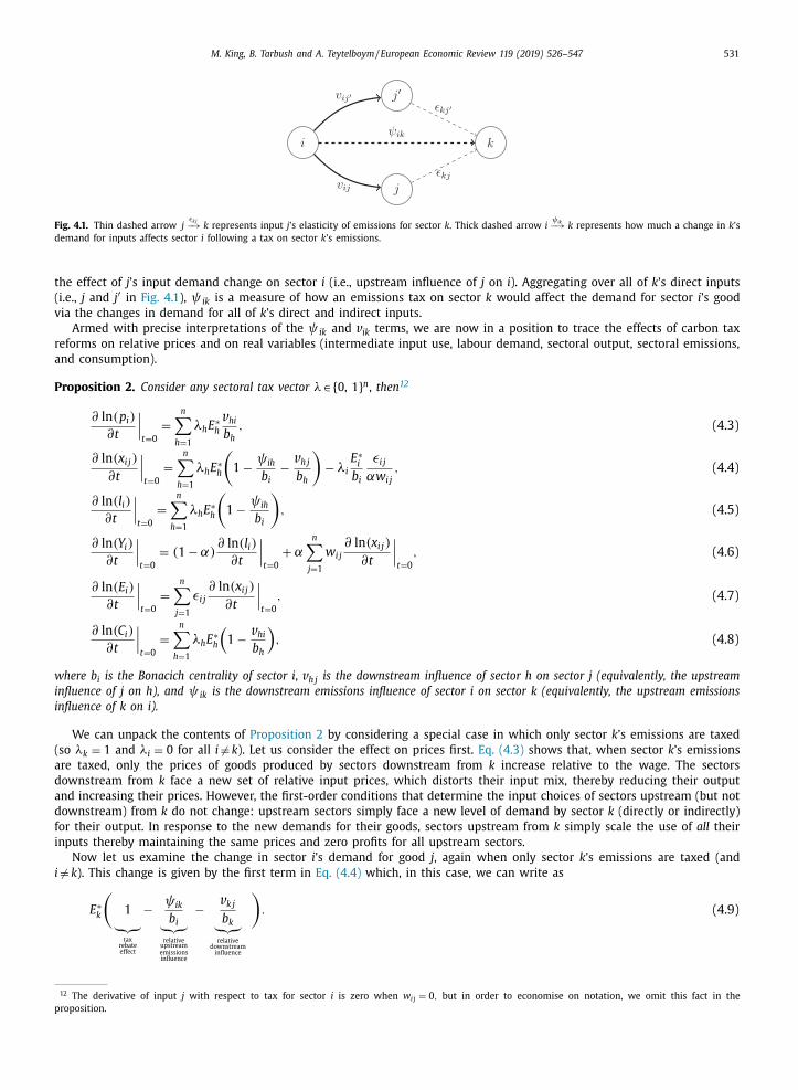
Fig. 4.1. Thin dashed arrow j εk j −→ k represents input j ’s elasticity of emissions for sector k . Thick dashed arrow i

ψ ik −→ k represents how much a change in k ’s

demand for inputs affects sector i following a tax on sector k ’s emissions.

the effect of j ’s input demand change on sector i (i.e., upstream influence of j on i ). Aggregating over all of k ’s direct inputs

(i.e., j and j ′ in Fig. 4.1 ), ψ ik is a measure of how an emissions tax on sector k would affect the demand for sector i ’s good

via the changes in demand for all of k ’s direct and indirect inputs.

Armed with precise interpretations of the ψ ik and v ik terms, we are now in a position to trace the effects of carbon tax

reforms on relative prices and on real variables (intermediate input use, labour demand, sectoral output, sectoral emissions,

and consumption).

Proposition 2. Consider any sectoral tax vector λ∈ {0, 1} n , then 12

∂ ln (p i )

∂t

∣∣∣t=0

=

n ∑

h =1

λh E ∗h

v hi

b h , (4.3)

∂ ln (x i j )

∂t

∣∣∣t=0

=

n ∑

h =1

λh E ∗h

(1 − ψ ih

b i − v h j

b h

)− λi

E ∗i

b i

εi j

αw i j

, (4.4)

∂ ln (l i )

∂t

∣∣∣t=0

=

n ∑

h =1

λh E ∗h

(1 − ψ ih

b i

), (4.5)

∂ ln (Y i )

∂t

∣∣∣t=0

= (1 − α) ∂ ln (l i )

∂t

∣∣∣t=0

+ αn ∑

j=1

w i j

∂ ln (x i j )

∂t

∣∣∣t=0

, (4.6)

∂ ln (E i )

∂t

∣∣∣t=0

=

n ∑

j=1

εi j

∂ ln (x i j )

∂t

∣∣∣t=0

, (4.7)

∂ ln (C i )

∂t

∣∣∣t=0

=

n ∑

h =1

λh E ∗h

(1 − v hi

b h

), (4.8)

where b i is the Bonacich centrality of sector i , v h j is the downstream influence of sector h on sector j (equivalently, the upstream

influence of j on h), and ψ ik is the downstream emissions influence of sector i on sector k (equivalently, the upstream emissions

influence of k on i).

We can unpack the contents of Proposition 2 by considering a special case in which only sector k ’s emissions are taxed

(so λk = 1 and λi = 0 for all i � = k ). Let us consider the effect on prices first. Eq. (4.3) shows that, when sector k ’s emissions

are taxed, only the prices of goods produced by sectors downstream from k increase relative to the wage. The sectors

downstream from k face a new set of relative input prices, which distorts their input mix, thereby reducing their output

and increasing their prices. However, the first-order conditions that determine the input choices of sectors upstream (but not

downstream) from k do not change: upstream sectors simply face a new level of demand by sector k (directly or indirectly)

for their output. In response to the new demands for their goods, sectors upstream from k simply scale the use of all their

inputs thereby maintaining the same prices and zero profits for all upstream sectors.

Now let us examine the change in sector i ’s demand for good j , again when only sector k ’s emissions are taxed (and

i � = k ). This change is given by the first term in Eq. (4.4) which, in this case, we can write as

E ∗k

(1 ︸︷︷︸ tax

rebate effect

− ψ ik

b i ︸︷︷︸ relative

upstream emissions influence

− v k j

b k ︸︷︷︸ relative

downstream influence

). (4.9)

12 The derivative of input j with respect to tax for sector i is zero when w i j = 0 , but in order to economise on notation, we omit this fact in the

proposition.

532 M. King, B. Tarbush and A. Teytelboym / European Economic Review 119 (2019) 526–547

The term E ∗k

outside the parentheses states the obvious: the higher the emissions of sector k , the greater its impact on

the whole network. The first term inside the parentheses is the tax rebate effect (aggregate demand channel): since the

consumer has a higher income, she can consume more of good i thereby increasing sector i ’s demand for all its inputs.

The second term is the relative upstream emissions influence of sector k on sector i . The reduction in sector k ’s demand

for inputs dampens sector i ’s demand for inputs. However, the magnitude of this effect is attenuated by the sales (Bonacich

centrality) of i . The third term is the relative downstream influence of sector k on sector j . When sector k is taxed, its output

price rises. This raises the price of downstream sector j ’s good which, in turn, reduces i ’s demand for good j . The magnitude

of this effect is attenuated by the sales of sector k since taxing the emissions of a sector with large sales (relative to a fixed

level of emissions E ∗k

) will have a small impact on its price and therefore on the prices of its downstream sectors.

To understand the relevance of the final term in Eq. (4.4) we need to consider a setting in which sector i ’s emissions are

among those that are taxed (so λi = 1 ). This final term is always negative and measures the additional self-distortion to the

first-order conditions of sector i from a tax on its own emissions.

Let us now look at the effects of a tax reform on the remaining variables in the case in which only sector k ’s emissions

are taxed. The labour demand of sector i is affected only by the tax rebate effect and by the relative upstream emissions

influence of k on i (see Eq. (4.5) ). Since the wage is our anchor price, it remains unchanged, and therefore there is no down-

stream (or price) effect of an emissions tax on labour demand. The impact of the tax reform on sectoral output and sectoral

emissions can be decomposed into weighted sums of changes in the use of the relevant inputs (see Eqs. (4.6) and (4.7) ).

In the case of output, the weights are simply expenditure shares on factors of production, and, in the case of emissions,

the weights are emissions elasticities. Finally, from Eq. (4.8) , we can observe that the change in the consumption of good i

depends only on the tax rebate effect and on the relative downstream influence of sector k on sector i . This is because the

consumer cares only about relative prices of goods and only the prices of goods produced by sectors downstream from k

change following an emissions tax on k .

Finally, we turn to the effects of incremental carbon taxation on utility and real GDP. The effect of incremental taxation

on the consumer’s utility is zero because the tax rebate exactly offsets the relative price changes. Indeed, by Eq. (4.8) and

the definition of Bonacich centrality,

∂ ln (U)

∂t

∣∣∣t=0

=

n ∑

i =1

1

n

∂ ln (C i )

∂t

∣∣∣t=0

=

n ∑

h =1

λh E ∗h

n ∑

i =1

1

n

(1 − v hi

b h

)= 0 . (4.10)

Since real GDP is equal to utility by Proposition 1 , an incremental emissions tax has no effect on real GDP. Of course, if taxes

were away from the margin or if utility were a function of emissions, then emissions taxation might have consequences for

real GDP and welfare.

5. Targeted carbon tax reforms

In this section we analyse the impact of carbon tax reforms on aggregate emissions. We first characterise the effect of

taxing the emissions of individual sectors. We introduce two new concepts: key sectors and aggregate emissions impact . We

then consider the effects of taxing the emissions of any set of sectors. Finally, we draw implications for policy.

5.1. Key sectors: taxing the emissions of individual sectors

Let us first characterise the effect of taxing the emissions of one sector on aggregate emissions. Define ϒ i to be the

aggregate emissions impact of sector i , that is,

ϒi =

∂ ln (E)

∂t

∣∣∣∣λ = e i t = 0

,

where e i denotes the i th standard basis vector. Of course, the aggregate emissions impact of a sector i is different from

the change in the emissions of sector i following a carbon tax on i alone (that is, ∂ ln (E) ∂t

∣∣λ = e i t = 0

� =

∂ ln (E i )

∂t

∣∣λ = e i t = 0

). The following

proposition characterises the aggregate emissions impact of sector i .

Proposition 3. The aggregate emissions impact of sector i is given by

ϒi = E ∗i −n ∑

j=1

E ∗i E ∗

j

E ∗

(ψ ji

b j +

ψ i j

b i

)− (E ∗

i ) 2

E ∗

(

n ∑

j=1

ε2 i j

αw i j b i

)

. (5.1)

Let us now unpack the terms of Eq. (5.1) . The first term is simply the tax rebate effect. The higher the emissions of sector

i , the greater the amount of tax revenue that the government can raise following a tax. As before, this effect makes the con-

sumer wealthier which induces greater spending across the economy, higher output, and higher emissions. This is the only

positive term in the expression. 13 We call the second term sector i ’s intersectoral emissions influence : it is a weighted sum

13 In a partial equilibrium setting in which only a fraction of the tax is rebated to the consumer, this term would be scaled down correspondingly.

M. King, B. Tarbush and A. Teytelboym / European Economic Review 119 (2019) 526–547 533

of relative upstream and relative downstream emissions influences. Note that the relative downstream emissions influence

part is new to Proposition 3 (and did not appear in Eq. (4.4) of Proposition 2 ): when i ’s emissions are taxed, i ’s price rises

which distorts the input mix of its downstream sectors, thereby reducing their output and their emissions. The final term

comes from the familiar self-distortion to sector i when its own emissions are taxed (cf. Eq. (4.4) ).

In general, ϒ i , the aggregate emissions impact of sector i , can be positive or negative (in the sense that one can construct

theoretical examples in which some sectors have a strictly positive aggregate emissions impact and others have a strictly

negative impact). It should be clear that if the size of the tax rebate term outweighs the intersectoral emissions influence

and the self-distortion terms then the aggregate emissions impact of a sector will be positive.

Definition 6. Sector i is a key sector if its aggregate emissions impact is strictly negative.

Using Eq. (5.1) , we can see that a sector is more likely to be a key sector if it has a large intersectoral emissions in-

fluence or high emissions. Indeed, the aggregate emissions impact of sector i is generally inverse-U-shaped in sector i ’s

emissions. So, for low levels of sector i ’s emissions, the tax rebate term might outweigh the self-distortion term (potentially

rendering the aggregate emissions impact positive), whereas when sector i ’s emissions are sufficiently high, the (squared)

self-distortion term will dominate the other two effects.

To appreciate how intersectoral linkages affect the relationship between a sector’s emissions and its aggregate emissions

impact, let us consider what happens in an economy without any intersectoral linkages.

Proposition 4. Assume that W = I. Then, for any key sectors i and j ,

| ϒi | ≥ | ϒ j | if and only if E ∗i ≥ E ∗j .

When W = I, there are no intersectional linkages in the economy. Each sector uses only labour and its own output as

inputs. 14 In this case, εii = 1 for all sectors. When a tax is imposed on the emissions of sector k , the price of good k rises

relative to all other prices, while k ’s input use, output, emissions, and the consumption of good k all decrease. Conversely,

the input use, output, and consumption of all other goods ( i � = k ) rise. Following a sectoral carbon tax on k , the consumer

spends the tax rebate equally on the goods of all sectors and the emissions of all sectors but k rise. Therefore, when the

emissions of a high-emitting sector k are taxed, the reduction in k ’s emissions is large and, at the same time, the consumer

spends the tax rebate on the goods of sectors less-emitting on average than k . In fact, Proposition 4 shows that, in this

economy, a key sector has a higher aggregate emissions impact (in absolute terms) than another key sector if and only if it

has higher emissions in the zero-tax equilibrium. Therefore, if a policymaker were interested in reducing emissions by taxing

one sector, they could simply look at the key sector with the greatest sectoral emissions. In the presence of intersectoral

linkages, however, Proposition 4 no longer holds. 15 Therefore, the sector with the highest aggregate emissions impact might

not have the highest sectoral emissions in general. 16

5.2. Taxing the emissions of multiple sectors

Having characterised the effects of taxing the emissions of any single sector, we now consider the effect of taxing the

emissions of any set of sectors. For any set of sectoral emissions taxes μ∈ {0, 1} n we define the aggregate emissions impact

of a carbon tax reform as

ϒ(μ) =

∂ ln (E)

∂t

∣∣∣∣λ = μt = 0

.

Notice that ϒ i ≡ϒ( e i ). The effect on aggregate emissions of taxing the emissions of any set of sectors can be linearly de-

composed into the aggregate emissions impacts of individual sectors.

Proposition 5. For any sectoral tax vector λ∈ {0, 1} n ,

ϒ(λ) =

n ∑

i =1

λi ϒi . (5.2)

14 Acemoglu et al. (2017) also consider a counterfactual “simple economy” without intersectoral linkages by setting α = 0 . This implies that every sector

uses only labour as an input. This counterfactual economy is less appropriate in our setting since we have assumed that emissions do not depend on labour

directly so this economy would produce no emissions. 15 In general, Proposition 4 would also break down in the presence of heterogeneity in consumer preferences, sectoral production functions, or sectoral

emissions elasticities. See Remark 1 after the proof of Proposition 4 in Appendix C . 16 In Appendix E , we study an extension of the economy without intersectoral linkages considered in Proposition 4 that allows for heterogeneity in

the consumer’s preferences. As consumer expenditure shares are no longer assumed to be equal, the monotonic relationship between sectoral emissions

and aggregate emissions impacts predicted in Proposition 4 no longer holds. Yet, we show that accounting for intersectoral linkages remains important for

calculating aggregate emissions impacts. To see this, we match sectoral sales of the interconnected economy with those of the economy without linkages by

adjusting the consumer’s preference weights. Despite having identical sales, the aggregate emissions impacts are quantitatively and qualitatively different

in the two economies.

534 M. King, B. Tarbush and A. Teytelboym / European Economic Review 119 (2019) 526–547

As Proposition 5 shows, the impact of a multi-sector carbon tax reform on aggregate emissions is the sum of the ag-

gregate emissions impacts of each taxed sector. In other words, the aggregate emissions impact of taxing the emissions of

sectors i and k is equal to the aggregate emissions impact of sector i plus the aggregate emissions impact of sector k . There-

fore, taxing the emissions of any key sector will reduce emissions while taxing the emissions of any additional non-key

sector will dampen this reduction.

5.3. Policy implications

Let us consider the implications of our analysis for policy. We say that the most effective carbon tax reforms are the sets

of incremental sectoral taxes that produce the greatest reduction in aggregate emissions (around the zero-tax equilibrium).

Let us define the most effective carbon tax reforms formally.

Definition 7. The most effective carbon tax reforms are vectors λ∗ which satisfy

λ∗ ∈ arg min

μ∈{ 0 , 1 } n

{

ϒ(μ) such that ϒ(μ) < 0

}

. (5.3)

Recall that any carbon tax reform leads to no loss in real GDP or utility, but the most effective carbon tax reforms will

lead to the greatest reduction in emissions at the margin. The most effective carbon tax reform is, of course, not the socially

optimal carbon tax; instead we want to find the steepest gradient of emissions in the direction of an incremental tax.

Taxing the emissions of all sectors will unambiguously reduce aggregate emissions as the following proposition shows.

Proposition 6. Taxing the emissions of all sectors reduces aggregate emissions, i.e.,

ϒ( 1 ) ≤ 0 . (5.4)

However, because some sectors may have a positive aggregate emissions impact, taxing the emissions of all sectors might

not constitute the most effective carbon tax reform, as the following corollary of Proposition 5 shows.

Corollary 1. In the most effective carbon tax reform, sector i’s emissions are taxed if and only if i is a key sector. 17

Corollary 1 gives a stark characterisation of the most effective carbon tax reform by focusing only on whether a sector

is key or non-key. However, in practice, due to political or technological constraints, the most effective carbon tax reform

may not be achievable. Nevertheless, the magnitudes of aggregate emissions impacts (derived in Proposition 3 ) can serve

as a guide to the policymaker who is interested in effective emissions reduction. The policymaker can use the aggregate

emissions impacts of sectors to rank sectors according to their importance in reducing emissions in the economy. And,

recalling our discussion of Proposition 4 , in the presence of intersectoral linkages, the policymaker cannot simply rely on

a ranking by sectoral emissions as a basis for the most effective carbon tax reform because sectors with highest emissions

might not have the greatest aggregate emissions impact (in absolute value). As Proposition 5 shows, the greatest emissions

reduction following a carbon tax reform, is achieved by targeting as many of the key sectors that have the highest aggregate

emissions impact (in absolute value) as possible. 18

6. Calibration

We now illustrate our main results by tracing the effects of carbon tax reforms in a version of our model that is cali-

brated to real-world data. In the calibration, we will maintain our competitive equilibrium assumption but introduce more

heterogeneity in the sectoral production functions and in the representative consumer’s preferences. We therefore assume

that

Y i = l 1 −αi

i

n ∏

j=1

x αi w i j

i j , (6.1)

17 If the government were also able to subsidise certain sectors then the most effective carbon policy reform would be

λ∗ ∈ arg min μ∈{−1 , 0 , 1 } n

{ ϒ(μ) such that ϒ(μ) < 0 and T > −ω

} .

That is, the government can choose which sectors to tax and subsidise subject to the constraint that the consumer’s income remains strictly positive. The

solution to this problem is an immediate consequence of Proposition 5 : tax all the key sectors and subsidise as many sectors with the largest positive

aggregate emissions impacts as possible. The reason subsidies for non-key sectors reduce emissions in our model is that the reduction in the consumer’s

income (the negative tax rebate effect) exceeds the (positive) emissions influence and self-distortion terms. This policy reform relies heavily on the as-

sumption of fixed technology: if firms can adjust their production functions, they could easily exploit the subsidy while increasing emissions. 18 Rather than having to optimise over 2 n possible subsets of taxed sectors!

M. King, B. Tarbush and A. Teytelboym / European Economic Review 119 (2019) 526–547 535

where αi ∈ (0, 1) for all sectors i , and that

U(C 1 , . . . , C n ) =

n ∏

i =1

C γi

i , (6.2)

where without loss of generality ∑ n

i =1 γi = 1 . Moreover, we assume that the emissions function for each sector i is linear,

i.e.,

E i (x 1 i , . . . , x ni ) =

n ∑

j=1

ηi j x i j , (6.3)

where ηij ≥ 0 measures the emissions intensity of sector i ’s use of input j .

To calibrate αi , w i j , γ i , and ηij , we use data from the Global Trade Analysis Project (GTAP 8) database which con-

tains consistent information on input-output and emissions networks for 57 sectors across many developing and developed

economies in 2007 ( Narayanan et al., 2012 ). 19

In particular, we use data on sectoral sales and intersectoral spending patterns to calibrate the production and consump-

tion sides of our economy, and we use the data on intersectoral emissions to back out sectoral carbon emissions (in tons)

as well as the emissions elasticities. The details of our calibration method are given in Appendix D .

We should stress that our calibration is for illustrative purposes only and we ignore important factors such as other taxes

and government spending, international trade, and capital investment. We focus on the United States and Pakistan. We chose

these countries mainly because they have: (i) a relatively low fraction of trade/GDP (28% and 33% of GDP, respectively); (ii)

relatively low general government final consumption expenditure (15% and 10% of GDP, respectively); and (iii) no substantial,

explicit, and nationwide carbon taxes. 20

Since our comparative static results apply only to incremental taxes, we calculate the effects of a small carbon tax of

$10 per ton of carbon emissions. We do not suggest that this is an appropriate carbon tax. The World Bank High-Level

Commission on Carbon Prices led by Nicholas Stern and Joseph Stiglitz recommended a tax of between $40 and $80 per ton

of CO 2 emissions by 2020 ( High-Level Commission on Carbon Prices, 2017 ), which, adjusting for inflation, would correspond

to roughly $32–$64 per ton of carbon in 2007. Our derivative calculations may not extrapolate well to analysing the effects

of carbon taxes of this magnitude. To estimate the percentage change in aggregate emissions as a result of the $10 tax, we

extrapolate linearly around the estimated zero-tax equilibrium using an expression for the aggregate emissions impact that

is derived for the generalised model in Appendix D .

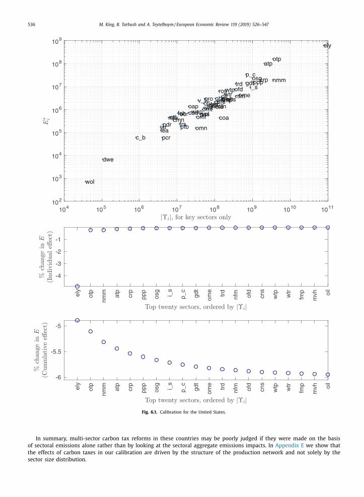
Panel 1 in Fig. 6.1 plots sectoral emissions against the absolute value of aggregate emissions impacts for all sectors

in the United States (on a log scale). 21 We can see that the emissions and the aggregate emissions impact of the elec-

tricity production sector are higher than those of any other sector. In general, however, the relationship between emis-

sions and aggregate emissions impacts is not one-to-one: for example, the air transport sector is more polluting than the

non-metallic minerals sector, yet the aggregate emissions impact of the latter exceeds that of the former. 22 Panel 2 in

Fig. 6.1 shows the estimated percentage reduction in aggregate emissions from individually taxing the emissions of any of

the top twenty key sectors with the highest aggregate emissions impacts. For example, taxing the emissions of the electric-

ity production sector alone gives a 4.893 percent reduction in aggregate emissions. Panel 3 in Fig. 6.1 shows the estimated

percentage reduction in aggregate emissions of cumulatively taxing the emissions of the key sectors with the highest ag-

gregate emissions impacts. For example, taxing the emissions of the electricity sector alone gives a 4.893 percent reduction

in emissions while taxing the emissions of the electricity and transport sectors together gives a 5.106 percent reduction

in emissions. 23 Note that taxing the emissions of the top twenty sectors (out of 57) with the highest aggregate emis-

sions impacts delivers most of the aggregate emissions reduction (of around 6.05%) from an economy-wide $10 carbon tax

reform.

Panel 1 in Fig. 6.2 plots sectoral emissions against the absolute value of aggregate emissions impacts for all the key

sectors in Pakistan (on a log scale). 24 The emissions of the electricity production sector are around three times higher than

those of the non-metallic minerals sector. However, the aggregate emissions impact of the non-metallic minerals sector

is approximately four times higher than that of the electricity production sector. From Panels 2 and 3, one can see that,

similarly to the US, taxing the emissions of the top twenty sectors would deliver most of the carbon reduction (of 4.35%)

from an economy-wide $10 carbon tax reform.

19 The data are available at https://www.gtap.agecon.purdue.edu/databases/archives.asp . 20 World Bank Open Data: https://data.worldbank.org/ . 21 Sector codes and descriptions are available on the GTAP website: https://www.gtap.agecon.purdue.edu/databases/v8/v8 _ sectors.asp . 22 ely corresponds to “Electricity: production, collection and distribution”. nmm corresponds to “Non-Metallic Minerals: cement, plaster, lime, gravel,

concrete”. atp corresponds to “Air transport”. otp corresponds to “Other Transport: road, rail; pipelines, auxiliary transport activities; travel agencies”,

which we simply refer to as “transport”. 23 In Appendix D , we explain why the estimated percentage change in aggregate emissions from a tax on the emissions of the electricity (4.893%)

and transport sectors (0.224%) individually does not add up exactly to the estimated percentage change from a tax on their emissions jointly (i.e.,

4.893+0.224 � = 5.106%). 24 The only non-key sector – dwellings – has zero recorded emissions and therefore an aggregate emissions impact of zero. While theoretically possible,

we do not find empirical evidence of non-key sectors with a strictly positive aggregate emissions impact in our data.

536 M. King, B. Tarbush and A. Teytelboym / European Economic Review 119 (2019) 526–547

104 105 106 107 108 109 1010 1011102

103

104

105

106

107

108

109

pdr

wht

grov_f

osd

c_b

pfb

ocrctl

oap

rmk

wol

frs

fshcoa

oil

gas

omn

cmtomtvol

mil

pcr

sgr

ofd

b_ttexwap

lea

lum

pppp_c

crp nmmi_s

nfmfmpmvh

otnele

ome

omf

ely

gdt

wtrcns

trd

otp

wtp

atp

cmn

ofi

isr

obsros

osg

dwe

ely

otp

nmm

atp

crp

ppp

osg

i_s

p_c

gdt

ome

trd

nfm ofd

cns

wtp wtr

fmp

mvh oi

l

-4

-3

-2

-1

ely

otp

nmm

atp

crp

ppp

osg

i_s

p_c

gdt

ome

trd

nfm ofd

cns

wtp wtr

fmp

mvh oi

l

-6

-5.5

-5

Fig. 6.1. Calibration for the United States.

In summary, multi-sector carbon tax reforms in these countries may be poorly judged if they were made on the basis

of sectoral emissions alone rather than by looking at the sectoral aggregate emissions impacts. In Appendix E we show that

the effects of carbon taxes in our calibration are driven by the structure of the production network and not solely by the

sector size distribution.

M. King, B. Tarbush and A. Teytelboym / European Economic Review 119 (2019) 526–547 537

101 102 103 104 105 106 107 108 109100

101

102

103

104

105

106

107

pdrwht

gro

v_f

osd

c_b pfbocr

ctloap

rmk

wolfrs

fsh

coa

oil

gas

omn

cmt

omt

volmil

pcr

sgr

ofd

b_t tex

wap

lea

lum

pppp_c

crpnmm

i_s

nfm

fmp

mvh

otn

ele

ome

omf

ely

gdtwtr

cns

trd

otp

wtp

atp

cmn

ofi

isr

obsrososg

nmm ely

ome

i_s

otp

nfm ele

crp

cns

omn

osg

omf

ppp

gdt

mvh atp

trd

tex

wtp

lum

-2

-1.5

-1

-0.5

0

nmm ely

ome

i_s

otp

nfm ele

crp

cns

omn

osg

omf

ppp

gdt

mvh atp

trd

tex

wtp

lum

-4

-3.5

-3

-2.5

Fig. 6.2. Calibration for Pakistan.

7. Conclusion

This paper formally analyses carbon taxes in the presence of intersectoral linkages. Our results highlight the importance

of considering general equilibrium effects when implementing carbon tax reforms. We provide closed-form expressions for

the network effects of carbon tax reforms on output, labour demand, consumption, intermediate input use, as well as

538 M. King, B. Tarbush and A. Teytelboym / European Economic Review 119 (2019) 526–547

aggregate and sectoral emissions. We show that a carbon tax reform imposed on all sectors may not reduce aggregate

emissions by the greatest amount. The most effective carbon tax reform involves taxing key sectors: those with a negative

aggregate emissions impact. Taxing additional non-key sectors dampens the reduction in aggregate emissions due to the

tax rebate effect. We also showed that the magnitudes of the aggregate emissions impacts—rather than sectoral emissions

alone—matter a great deal for any effective carbon tax reform.

Our formal analysis is valid only for small changes in carbon taxes: since the system defining our economy is non-linear

in the presence of distortionary taxes, the derivatives that we present may not extrapolate well to large carbon taxes. How-

ever, the basic logic of our results—that targeted sectoral taxation might be more effective than economy-wide taxation—

might well extend to non-marginal tax changes. This suggests that the quantitative gains of adopting targeted sectoral tax-

ation should be considered as a policy scenario in more sophisticated integrated assessment models.

A marginal analysis similar to the one in this paper could be used to examine two policy levers beyond the sector-

specific emissions taxes that we have focussed on. Firstly, commonly advocated and used cap-and-trade schemes might have

complex aggregate and distributional effects in the presence of intersectoral linkages ( Montgomery, 1972; Stavins, 2008;

Hepburn et al., 2013 ). Modifying the model to analyse a cap-and-trade scheme would allow us to investigate the economy-

wide impacts of two policy changes: either tightening the aggregate emissions cap, or making changes to the allocation of

sector-specific emissions permits. 25 Secondly, one could also consider direct taxation of polluting inputs in which each sector

i could be subjected to input taxes (or subsidies) τ ij that apply to the dirtiness of each input ( ∂E i ∂x i j

x i j ). 26

Moreover, in an international trade version of our model, input-specific taxes could allow us to trace the effects of border

carbon adjustments ( Fischer and Fox, 2012; Helm et al., 2012 ) and to investigate carbon leakage ( Babiker, 2005 ).

There are several ways to enrich the production side of our economy. One could include firm profits ( Baqaee, 2015;

Huremovic and Vega-Redondo, 2016 ), financial frictions ( Bigio and La’O, 2016 ) or other fundamental market distortions ( Liu,

2017 ), firm entry and exit ( Baqaee, 2015 ), dynamics and unemployment ( Baqaee, 2016 ), distributional concerns ( Klenert

et al., 2016 ), international trade ( Antweiler et al., 2001; Davis and Caldeira, 2010; Bosker and Westbrock, 2014 ), and produc-

tion network formation ( Acemoglu and Azar, 2017; Oberfield, 2018 ). Further work could also examine the extent to which

our results are affected by existing taxes ( Goulder, 1995; Bovenberg and Goulder, 1996; Parry et al., 1999 ), partial rebates of

tax revenue ( Metcalf, 2009 ), and technological progress induced by changes in relative prices ( Di Maria and Van der Werf,

2008 ).

Appendix A. Proof of Proposition 1

The steps of this proof closely follow Acemoglu et al. (2015) .

The consumer’s problem. Due to Cobb-Douglas preferences, the consumer spends a fixed proportion of her income on each

good:

p i C i =

1

n

(ω + T ) . (A.1)

Sectoral profit maximisation. The first-order conditions of (a representative firm in) sector i are given by 27

p i αw i j

Y i x i j

= p j + λi tω

∂E i ∂x i j

, (A.2)

p i (1 − α) Y i l i

= ω. (A.3)

Equilibrium prices. For each sector i , define i ’s sales as s i = p i Y i , and let z i j = λi tx i j ∂E i ∂x i j

. Then we can re-write the sectoral

first-order conditions as

s i αw i j = p j x i j + ωz i j , (A.4)

s i (1 − α) = ωl i . (A.5)

Now take a log of the production function in Eq. (2.1) to obtain

ln (Y i ) = (1 − α) ln (l i ) + αn ∑

j=1

w i j ln (x i j ) . (A.6)

25 Suppose that the government allocated each sector i an emissions permit allowance σ i Q , where Q is the overall emissions cap and σ i is sector i ’s share

of the cap ( ∑ n

i =1 σi = 1 ). Permits are competitively traded across firms at price p Q and the market for emissions permits clears when ∑ n

i =1 E i = Q . Hence (a

representative firm in) each sector i chooses l i and x ij to maximise p i Y i −∑ n

j=1 p j x i j − ωl i − p Q E i + p Q σi Q . 26 In the presence of polluting input taxation, (a representative firm in) each sector i chooses l i and x ij to maximise p i Y i −

∑ n j=1 p j x i j − ωl i −

∑ n j=1 τi j

∂E i ∂x i j

x i j .

27 We take the second-order conditions to be satisfied, e.g., when E i is linear.

M. King, B. Tarbush and A. Teytelboym / European Economic Review 119 (2019) 526–547 539

Plug in the first-order conditions Eqs. (A.4) and (A.5) to get

ln (Y i ) = (1 − α) ln (s i (1 − α)) − (1 − α) ln (ω) + αn ∑

j=1

w i j ln (s i αi w i j − ωz i j ) − αn ∑

j=1

w i j ln (p j ) . (A.7)

Subtract ln ( s i ) from both sides and then multiply both sides by −1 to obtain

ln (p i ) = ln (s i ) − (1 − α) ln (s i (1 − α)) + (1 − α) ln (ω) − αn ∑

j=1

w i j ln (s i αw i j − ωz i j ) + αn ∑

j=1

w i j ln (p j ) . (A.8)

At t = 0 Eq. (A.8) becomes

ln (p ∗i ) = −(1 − α) ln (1 − α) − α ln (α) + (1 − α) ln (ω) − αn ∑

j=1

w i j ln (w i j ) + αn ∑

j=1

w i j ln (p ∗j ) . (A.9)

Let θ = (1 − α) ln (1 − α) + α ln (α) . We can now re-write Eq. (A.9) in matrix form

ln (p ∗) = −θ1 − α(W ◦ ln (W )) 1 + (1 − α) ln (ω) 1 + αW ln (p ∗) , (A.10)

where ◦ denotes the Hadamard product. Solving Eq. (A.10) one obtains

ln (p ∗) = −V

′ [ θ1 + α(W ◦ ln (W )) 1 − (1 − α) ln (ω) 1 ] . (A.11)

The i th entry of the equilibrium log price vector is therefore given by

ln (p ∗i ) = −θn ∑

j=1

v ji − αn ∑

j=1

v ji n ∑

h =1

w jh ln (w jh ) + (1 − α) n ∑

j=1

v ji ln (ω) . (A.12)

Now notice that V ′ 1 =

(I +

∑ ∞

k =1 αk W

k )1 = (1 − α) −1 1 , where the second step follows from the fact that W is row

stochastic. It follows that ∑ n

j=1 v ji = (1 − α) −1 for each i . Therefore,

ln (p ∗i ) = − θ

1 − α− α

n ∑

j=1

v ji n ∑

h =1

w jh ln (w jh ) + ln (ω) . (A.13)

Equilibrium sales. Multiply both sides of the market clearing condition in Eq. (3.2) by p i to obtain that

p i Y i = p i C i +

n ∑

j=1

p i x ji . (A.14)

Plugging in the consumer’s demands from Eq. (A.1) we have

s i =

1

n

(ω + T ) +

n ∑

j=1

p i x ji . (A.15)

Using the sectoral first-order conditions in Eqs. (A.4) and (A.5) we get

s i =

1

n

(ω + T ) + αn ∑

j=1

s j w ji −n ∑

j=1

z ji ω. (A.16)

In matrix form,

s =

1

n

(ω + T ) 1 + αW

′ s − ωZ ′ 1 . (A.17)

And so,

s = V

[ 1

n

(ω + T ) 1 − ωZ ′ 1

] . (A.18)

The i th entry of the equilibrium sales vector is therefore given by

s i = (ω + T ) b i − ω

n ∑

j=1

v i j

n ∑

h =1

z h j . (A.19)

Clearly, when t = 0 , we have that s i = ωb i . We can therefore use this result in conjunction with the equilibrium prices in

Eq. (A.13) and the sectoral first-order conditions in Eqs. (A.4) and (A.5) to obtain the results stated in Proposition 1 . The

fact that C ∗i

= ω/ (np ∗i ) follows from Eq. (A.1) . We obtain U

∗ by plugging the equilibrium consumption values into the utility

function.

540 M. King, B. Tarbush and A. Teytelboym / European Economic Review 119 (2019) 526–547

Appendix B. Derivatives of essential terms

For a given vector λ∈ {0, 1} n we need to evaluate the derivatives of consumption, labour, inputs, sectoral outputs, and

sectoral emissions with respect to t around the zero-tax benchmark. To do this, we first evaluate the derivatives of essential

terms such as z ij and T (among others) in this section. Throughout, ω is treated as a constant: we use it as the anchor-

ing price and therefore hold its level fixed. The proofs of the propositions that are stated in the main text are derived in

Appendix C .

Derivative of z ij . Recall that z i j = λi tx i j ∂E i ∂x i j

. Therefore

∂z i j

∂t = λi x i j

∂E i ∂x i j

+ λi t ∂

∂t

(x i j

∂E i ∂x i j

). (B.1)

Evaluating at t = 0 we obtain

∂z i j

∂t

∣∣∣t=0

= λi E ∗i εi j . (B.2)

Derivative of T . We have that T = tω

∑ n i =1 λi E i . Therefore

∂T

∂t

∣∣∣t=0

= ω

n ∑

i =1

λi E ∗i . (B.3)

Derivative of ln ( s i ). The equilibrium sales for sector i satisfy Eq. (A.19) . Therefore

∂s i ∂t

∣∣∣t=0

= b i ∂T

∂t

∣∣∣t=0

− ω

n ∑

j=1

v i j

n ∑

h =1

∂z h j

∂t

∣∣∣t=0

. (B.4)

Using Eqs. (B.3) and (B.2) , we obtain

∂s i ∂t

∣∣∣t=0

= ωb i

n ∑

h =1

λh E ∗h − ω

n ∑

j=1

v i j

n ∑

h =1

λh E ∗h εh j = ω

n ∑

h =1

λh E ∗h (b i − ψ ih ) . (B.5)

Notice that since s i = ωb i when t = 0 ,

∂ ln (s i )

∂t

∣∣∣t=0

=

1

ωb i

∂s i ∂t

∣∣∣t=0

=

n ∑

h =1

λh E ∗h

(1 − ψ ih

b i

). (B.6)

Derivative of ln (s i αw i j − ωz i j ) . This term appears in Eq. (A.8) which the equilibrium prices must satisfy. Taking a deriva-

tive of this term with respect to t yields

∂ ln (s i αw i j − ωz i j )

∂t =

∂s i ∂t

αw i j − ω

∂z i j

∂t

s i αw i j − ωz i j

. (B.7)

Evaluating at t = 0 , using Eqs. (B.6) and (B.2) and the fact that s i = ωb i at t = 0 , we obtain

∂ ln (s i αw i j − ωz i j )

∂t

∣∣∣t=0

=

1

ωb i

∂s i ∂t

∣∣∣t=0

− λi E ∗i εi j

αw i j b i =

∂ ln (s i )

∂t

∣∣∣t=0

− λi E ∗i εi j

αw i j b i . (B.8)

Appendix C. Proofs of Propositions 2–6

Proof of Proposition 2. Prices. Taking the derivative of Eq. (A.8) with respect to t yields

∂ ln (p i )

∂t = −

(

(1 − α) ∂ ln (s i (1 − α))

∂t + α

n ∑

j=1

w i j

∂ ln (s i αw i j − ωz i j )

∂t

)

+ αn ∑

j=1

w i j

∂ ln (p j )

∂t +

∂ ln (s i )

∂t . (C.1)

Using Eq. (B.8) , the term inside the parentheses evaluated at t = 0 is equal to

∂ ln (s i )

∂t

∣∣∣t=0

− λi E ∗i

b i

(

n ∑

j=1

εi j

)

=

∂ ln (s i )

∂t

∣∣∣t=0

− λi E ∗i

b i , (C.2)

where the second part follows from Euler’s theorem for homogeneous equations (emissions are homogeneous of degree

one). Substituting this back into Eq. (C.1) we obtain

∂ ln (p i )

∂t

∣∣∣t=0

=

λi E ∗i

b i + α

n ∑

j=1

w i j

∂ ln (p j )

∂t

∣∣∣t=0

. (C.3)

M. King, B. Tarbush and A. Teytelboym / European Economic Review 119 (2019) 526–547 541

Solving this linear system yields

∂ ln (p i )

∂t

∣∣∣t=0

=

n ∑

j=1

v ji λ j E

∗j

b j . (C.4)

Consumption. Taking a derivative of the consumer’s demand in Eq. (A.1) with respect to t yields

∂ ln (C i )

∂t =

1

C i

1

np i

(∂T

∂t − (ω + T )

∂ ln (p i )

∂t

). (C.5)

Evaluating at t = 0 , using the fact that C ∗i

= ω/ (np ∗i ) , and using Eqs. (B.3) and (C.4) , we obtain

∂ ln (C i )

∂t

∣∣∣t=0

=

1

ω

(∂T

∂t

∣∣∣t=0

− ω

∂ ln (p i )

∂t

∣∣∣t=0

)=

n ∑

j=1

λ j E ∗j

(1 − v ji

b j

). (C.6)

Labour demand. To obtain the result on labour demand, take a derivative of the log of both sides of Eq. (A.5) with respect

to t to obtain

∂ ln (l i )

∂t

∣∣∣t=0

=

∂ ln (s i (1 − α))

∂t

∣∣∣t=0

=

n ∑

h =1

λh E ∗h

(1 − ψ ih

b i

), (C.7)

where the second step follows from substitution of Eq. (B.6) .

Inputs. For the intermediate inputs take a derivative of the log of both sides of Eq. (A.4) with respect to t to obtain

∂ ln (x i j )

∂t

∣∣∣t=0

=

∂ ln (s i αw i j − ωz i j )

∂t

∣∣∣t=0

− ∂ ln (p j )

∂t

∣∣∣t=0

=

n ∑

h =1

λh E ∗h

(1 − ψ ih

b i − v h j

b h

)− λi E

∗i εi j

αw i j b i . (C.8)

where the second step follows from substitution of Eqs. (B.6) , (B.8) , and (C.4) .

Sectoral outputs and emissions. For sectoral outputs, observe that

∂ ln (Y i )

∂t

∣∣∣t=0

=

l ∗i

Y ∗i

· ∂Y i ∂ l i

∣∣∣t=0

∂ ln (l i )

∂t

∣∣∣t=0

+

n ∑

j=1

x ∗i j

Y ∗i

∂Y i ∂x i j

∣∣∣t=0

· ∂ ln (x i j )

∂t

∣∣∣t=0

. (C.9)

From the production function in Eq. (2.1) the elasticity of output i with respect to labour is (1 − α) while the elasticity of

output i with respect to intermediate input j is αw i j . This gives us the desired result. A similar derivation allows us to obtain

the derivative of log emissions. Namely,

∂ ln (E i )

∂t

∣∣∣t=0

=

n ∑

j=1

εi j

∂ ln (x i j )

∂t

∣∣∣t=0

. (C.10)

�

Proof of Propositions 3 and 5. Since E =

∑ n i =1 E i , the derivative of log aggregate emissions evaluated at t = 0 is given by

∂ ln (E)

∂t

∣∣∣t=0

=

n ∑

i =1

E ∗i

E ∗∂ ln (E i )

∂t

∣∣∣t=0

=

n ∑

i =1

E ∗i

E ∗

(

n ∑

j=1

εi j

∂ ln (x i j )

∂t

∣∣∣t=0

)

, (C.11)

where the second step follows from substitution of Eq. (C.10) . Plugging Eqs. (C.7) and (C.8) into the above and evaluating

yields

∂ ln (E)

∂t

∣∣∣t=0

=

n ∑

i =1

λi

∂ ln (E)

∂t

∣∣∣∣λ = e i t = 0

, (C.12)

where

∂ ln (E)

∂t

∣∣∣∣λ = e i t = 0

= E ∗i −n ∑

j=1

E ∗i E ∗

j

E ∗

(ψ ji

b j +

ψ i j

b i

)− (E ∗

i ) 2

E ∗

(

n ∑

j=1

ε2 i j

αw i j b i

)

. (C.13)

�

Proof of Proposition 4. When W = I it is easy to show that ψ i j = (1 − α) −1 if i = j and ψ i j = 0 if i � = j, and that b i =n −1 (1 − α) −1 for all i . The aggregate emissions impact of sector i is then

∂ ln (E)

∂t

∣∣∣∣λ = e i t = 0

= E ∗i −n

E ∗1 + α

α(E ∗i )

2 = E ∗i − κ(E ∗i ) 2 , (C.14)

542 M. King, B. Tarbush and A. Teytelboym / European Economic Review 119 (2019) 526–547

where κ =

n E ∗

1+ αα . The aggregate emissions impact of sector i is concave in E ∗

i with roots at 0 and 1/ κ and reaches a maxi-

mum somewhere in between. When E ∗i

> 1 /κ , the absolute value of the aggregate emissions impact is strictly increasing in

E ∗i

. A sector i is a key sector if E ∗i

> 1 /κ , so the result follows. �

Remark 1. Notice that, in the proof of Proposition 4 , if the aggregate emissions impact of sector i were dependent on i other

than through E ∗i

then ranking key sectors by their direct emissions and ranking key sectors by the absolute value of their

aggregate emissions impact will in general produce different results. For example, see the expression for a sector’s aggregate

emissions impact in the economy analysed in Appendix E (in which the consumer’s preferences are heterogeneous). We

should therefore expect different rankings whenever there is heterogeneity in intersectoral linkages, emissions elasticities,

consumer preferences, or production functions.

Proof of Proposition 6. Set λi = 1 for all i and let M = max i, j E ∗

i E ∗ εi j (and notice that M ≥ 0). Then by Eq. (C.11) ,

∂ ln (E)

∂t

∣∣∣t=0

≤ M

n ∑

i =1

n ∑

j=1

∂ ln (x i j )

∂t

∣∣∣t=0

. (C.15)

Since we set λi = 1 for each i , by Eq. (C.8) we also know that

∂ ln (x i j )

∂t

∣∣∣t=0

≤n ∑

h =1

E ∗h

(1 − ψ ih

b i − v h j

b h

)= E ∗ −

n ∑

h =1

E ∗h ψ ih

b i −

n ∑

h =1

E ∗h v h j

b h . (C.16)

Let us now sum the above expression over all j to obtain

n ∑

j=1

∂ ln (x i j )

∂t

∣∣∣t=0

≤ nE ∗ − n

n ∑

h =1

E ∗h ψ ih

b i −

n ∑

j=1

n ∑

h =1

E ∗h v h j

b h (C.17)

= nE ∗ − n

n ∑

h =1

E ∗h ψ ih

b i − n

n ∑

h =1

E ∗h (C.18)

= −n

n ∑

h =1

E ∗h ψ ih

b i . (C.19)

The second line follows from the fact that ∑ n

j=1 v h j = nb h . Since the term in the final line is weakly negative, we obtain the

desired result. �

Appendix D. Details of the calibration

One can follow the steps of Appendix A –Appendix C to show that, in the generalised model with heterogeneous con-

sumer preferences and heterogeneous labour shares in production, when t = 0 there is a unique competitive equilibrium

and it is characterised by

p ∗i = exp

(

−n ∑

j=1

ν ji ϑ j −n ∑

j=1

ν ji α j

n ∑

h =1

w jh ln (w jh ) +

n ∑

j=1

ν ji (1 − α j ) ln (ω)

)

, (D.1)

C ∗i = γi ω/p ∗i , (D.2)

s ∗i = ωβi , (D.3)

x ∗i j = s ∗i αi w i j /p ∗j , (D.4)

l ∗i = s ∗i (1 − αi ) /ω. (D.5)

The equilibrium emissions of sector i when t = 0 are given by E ∗i

= E i (x ∗i 1

, . . . , x ∗in ) . Furthermore, for any λ∈ {0, 1} n ,

∂ ln (E)

∂t

∣∣∣t=0

=

n ∑

i =1

λi

∂ ln (E)

∂t

∣∣∣∣λ = e i t = 0

, (D.6)

where the aggregate emissions impact of sector i is given by

∂ ln (E)

∂t

∣∣∣∣λ = e i t = 0

= E ∗i −n ∑

j=1

E ∗i E ∗

j

E ∗

(φ ji

β j

+

φi j

βi

)− (E ∗

i ) 2

E ∗

(

n ∑

j=1

ε2 i j

αi w i j βi

)

. (D.7)

The new terms are defined as follows: firstly, ϑ i = (1 − αi ) ln (1 − αi ) + αi ln (αi ) . Secondly, define A to be an n × n matrix

with the i th diagonal entry equal to α and every other entry equal to zero. Let V = (I − (AW ) ′ ) −1 , and define β = Vγ

i

M. King, B. Tarbush and A. Teytelboym / European Economic Review 119 (2019) 526–547 543

and � = VE ′ . One can verify that the derivative of utility with respect to tax at the zero-tax benchmark is still zero here.

Notice also that when for all i , γi = 1 /n and αi = α for some scalar α, then ϑ i = θ for all i , [ νi j ] = V = V = [ v i j ] , β = b, and

[ φi j ] = � = = [ ψ i j ] , which therefore recovers Eq. (5.1) , the expression for aggregate emissions impact when consumer

preferences and labour shares in production are homogeneous.

In order to calibrate the production and consumption sides of our model we use the GTAP variables TVOM , VDPM , and

VDFM . For any sector i and country c , TVOM ( i , c ) are the sales of domestic product (of i ) in country c at market prices.

The sales are made to households or to other sectors. For any sectors i and j in country c , VDFM ( i , j , c ) are the domestic

purchases by sector j of i ’s good in country c at market prices. For any sector i in country c , VDPM ( i , c ) are the domestic

purchases by households of i ’s good in country c at market prices. All the variables are measured in millions of dollars.

We describe how we calibrate the production and consumption sides of our economy below. The description applies in

the same way for each country. We therefore omit the country-indexing of the variables.

Since the consumer’s preference weight γ i is precisely the share of the consumer’s spending on the good produced by

sector i (see Eq. (D.2) ), we calibrate the consumer’s preference weights as γi = VDPM (i ) / ∑ n

i =1 VDPM (i ) . Similarly, for any sector

i , (1 − αi ) is precisely the spending of that sector on labour as a fraction of i ’s sales (see Eq. (D.5) ). Since ∑ n

j=1 VDFM ( j, i )

is a measure of i ’s spending on all intermediate inputs and TVOM (i ) measures i ’s sales, we obtain i ’s spending on labour as

TVOM (i ) − ∑ n j=1 VDFM ( j, i ) . It follows that we can calibrate αi via 1 − αi = ( TVOM (i ) − ∑ n

j=1 VDFM ( j, i )) / TVOM (i ) . Finally, having

calibrated αi we can work out the input–output matrix W as follows: since αi w i j is the spending of sector i on good j as a

fraction of i ’s sales (see Eq. (D.4) ), we obtain the calibration w i j = ( VDFM ( j, i ) / TVOM (i )) /αi .

The GTAP database contains information on imports and exports. We ignore international trade in our calibration: we

employ variables that report only spending by domestic households and sectors on goods produced by domestic sectors.

A full analysis that accounts for international trade is beyond the scope of this paper and may yield different numerical

results.

With the calibration for the production and consumption sides of the economy that is described above, we can work out

the equilibrium input values under a zero-tax regime. These can straightforwardly be calculated using Eqs. (D.1) and (D.4) .

Working out the equilibrium inputs allows us to calibrate the emissions side of our economy.

GTAP 8 contains data on sectoral carbon emissions as part of the core database. (GTAP 7 and its associated CO 2 emissions

data for 2004 have been used in previous studies of sectoral emissions; see, e.g., Davis and Caldeira, 2010 ). 28 For any sectors

i and j in country c , the variable MDF ( i , j , c ) measures the CO 2 emissions (in million tons) from purchases of domestic

energy commodity i by sector j in country c . 29 From this variable we create a new variable C (i, j, c) which measures carbon

emissions (in tons) from energy commodity i produced in country c and used by sector j in country c . We obtain this

variable via the transformation C (i, j, c) = (10 6 / 3 . 67) × MDF (i, j, c) , which uses the standard IPCC conversion factor. 30

Below, we describe how we calibrate the emissions side of our economy. Since the description applies in the same way

to each country, we once again drop the indexing by country. Since we have worked out the equilibrium input levels x ∗i j ,

we can use Eq. (6.3) to calibrate the emissions coefficients via ηi j = C ( j, i ) /x ∗i j

. In other words, the emissions that sector

i produces from using sector j ’s good as an input increases linearly with i ’s use of sector j ’s good. Finally, we obtain the

elasticities via εi j = ηi j x ∗i j /E ∗

i = C ( j, i ) /

∑ n j=1 C ( j, i ) .

Eq. (D.6) only provides us with a derivative for the log of aggregate emissions with respect to a tax reform. To estimate

the effect of targeted carbon tax reforms on aggregate emissions, we use the derivative at the zero-tax equilibrium to linearly

extrapolate the change in emissions from a given carbon tax change. To do this, let E ( t , λ) denote aggregate emissions when

the tax rate is t and the tax reform is λ. Now integrate Eq. (D.6) with respect to t and use the boundary condition that

aggregate emissions are given by E ∗ when t = 0 to obtain

E(t, λ) = E ∗ exp

{

t

n ∑

i =1

λi

∂ ln (E)

∂t

∣∣∣∣λ = e i t = 0

}

. (D.8)

It follows that for any tax reform λ∈ {0, 1} n the percentage change in aggregate emissions is given by (E(t, λ)

E ∗− 1

)× 100 . (D.9)

We use the equation above as our estimate of the percentage change in aggregate emissions when the tax rate is t . Strictly

speaking, our analytical results apply only for infinitessimal tax rates and our estimates may worsen rapidly with large tax

28 Lee (2008) provides details of the emissions estimation for GTAP 7. See also https://www.gtap.agecon.purdue.edu/resources/res _ display.asp?RecordID=

1143 . 29 The energy commodities in the dataset are: coal, crude oil, natural gas, petroleum products, and gas distribution. The dataset also reports emissions by

the government and by households. These emissions are ignored in the calibration reported here. 30 See http://www.ipcc.ch/ipccreports/tar/wg3/index.php?idp=477 .

544 M. King, B. Tarbush and A. Teytelboym / European Economic Review 119 (2019) 526–547

rates if the economy is highly non-linear. Note that in general (E(t, e i )

E ∗− 1

)+

(E(t, e j )

E ∗− 1

)� =

(E(t, e i + e j )

E ∗− 1

), (D.10)

i.e., the estimated percentage change in aggregate emissions of taxing individual sectors is not additive.

To work out the tax rate we need to normalise by nominal GDP. We estimate nominal GDP, or ω, using Eq. (D.3) since

ω =

∑ n i =1 s

∗i / ∑ n

i =1 βi =

∑ n i =1 TVOM (i ) /

∑ n i =1 βi , and we obtain a nominal GDP of roughly 15,445,088 million dollars for the

USA and of 162,421 million dollars for Pakistan. 31 For our $10 tax we therefore set the tax rate t to 10/(15445088 × 10 6 ) for

the USA and to 10/(162421 × 10 6 ) for Pakistan.

Appendix E. Role of intersectoral linkages

In this section we show that the aggregate emissions impacts estimated in Section 6 are not driven solely by the dis-

tribution of sector sizes; indeed, the structure of the whole production network matters for our results. To do this we

analyse an economy without intersectoral linkages (in which sectors use only labour and their own output as inputs) and

we calibrate consumer preference weights to match the sector size distribution of the interconnected economy of Pak-

istan examined in Section 6 . We show that, while the economy without an intersectoral network has the same sector

size distribution as the economy with an intersectoral network, the effects of sectoral carbon taxes differ across the two

economies.

The economy without intersectoral linkages. The production function of sector i is given by

Y i = l 1 −αi

x αii . (E.1)

This implies that there are no intersectoral linkages and W = I. The profit function of sector i is given by

πi = p i Y i − ωl i − p i x ii − λi tωE i , (E.2)

where E i = ηii x ii . The consumer’s preferences are given by

U(C 1 , . . . , C n ) =

n ∏

i =1

C γi

i , (E.3)

where ∑ n

i =1 γi = 1 . This economy is essentially identical to the one studied in Proposition 4 with the exception that there is

now heterogeneity in the consumer’s preference parameters. Using the notation of Appendix D we have that βi = γi / (1 − α) ;

φi j = 1 / (1 − α) if i = j and is zero otherwise; and εi j = 1 if i = j and is zero otherwise. Using Eq. (D.7) we therefore obtain

the aggregate emissions impact of sector i :

∂ ln (E)

∂t

∣∣∣∣λ = e i t = 0

= E ∗i −1 + α

αγi E ∗(E ∗i )

2 . (E.4)

When t = 0 , using Eq. (D.3) , the sales of sector i are given by ω

γi 1 −α .

Calibration of the economy without intersectoral linkages. We set nominal GDP, namely ω, to match the nominal GDP for

Pakistan’s economy that we obtained in Appendix D . We calibrate the emissions directly to match sectoral emissions in

Pakistan’s economy. Finally, we calibrate the consumer’s preference weights γ i by equating the sales of each sector i , ω

γi 1 −α ,

to the sales in Pakistan’s economy. In other words, γ i is proportional to the sales of sector i in Pakistan’s interconnected

economy and the labour share, 1 − α, is set to satisfy the normalisation that consumer preference weights sum to one. 32

This calibration allows us to compare the aggregate emissions impacts in the economies with and without intersectoral

linkages while keeping the sales distribution identical across the two economies.

Our results for the key sectors in the economy without intersectoral linkages are shown in Fig. E.1 . The top panel shows

that the aggregate emissions impacts of the key sectors in the economy without intersectoral linkages are correlated with

those of their counterparts in Pakistan’s interconnected economy. There are, however, important differences: when intersec-

toral linkages are accounted for (as was done for our calibration of Pakistan’s economy), the non-metallic minerals sector

is ranked first in terms of its aggregate emissions impact. When linkages are ignored, this sector becomes far less impor-

tant. The bottom panel of Fig. E.1 shows that the aggregate emissions impacts of the key sectors in the economy without

linkages are correlated with sectoral emissions, however, because of heterogeneity in consumer preferences the monotonic

relationship predicted in Proposition 4 is not present here (see Remark 1 in Appendix C ).

31 According to World Bank estimates, in 2007, the nominal GDP in the USA was 14,451,858 million dollars and the nominal GDP in Pakistan was 152,385

million dollars. See https://data.worldbank.org/indicator/NY.GDP.MKTP.CD?end=20 07&start=20 06&year _ high _ desc=true . 32 In this calibration, the labour share is 0.6. The aggregate labour share in Pakistan’s data is also 0.6.

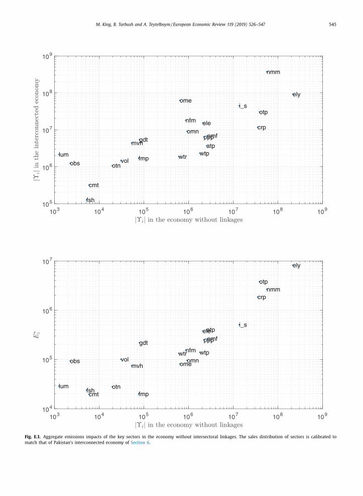
M. King, B. Tarbush and A. Teytelboym / European Economic Review 119 (2019) 526–547 545

103 104 105 106 107 108 109105

106

107

108

109

fsh

omn

cmt

vollum

ppp

crp

nmm

i_s

nfm

fmp

mvh

otn

ele

ome

omf

ely

gdt

wtr

otp

wtpatp

obs

103 104 105 106 107 108 109104

105

106

107

fsh

omn

cmt

vol

lum

ppp

crpnmm

i_s

nfm

fmp

mvh

otn

ele

ome

omf

ely

gdt

wtr

otp

wtp

atp

obs

Fig. E.1. Aggregate emissions impacts of the key sectors in the economy without intersectoral linkages. The sales distribution of sectors is calibrated to

match that of Pakistan’s interconnected economy of Section 6 .

546 M. King, B. Tarbush and A. Teytelboym / European Economic Review 119 (2019) 526–547

Supplementary material

Supplementary material associated with this article can be found, in the online version, at doi: 10.1016/j.euroecorev.2019.

08.001 .

References

Acemoglu, D., Azar, P.D., 2017. Endogenous production networks. National Bureau of Economic Research. Working Paper, https://www.nber.org/papers/

w24116 . Acemoglu, D. , Carvalho, V. , Ozdaglar, A. , Tahbaz-Salehi, A. , 2012. The network origins of aggregate fluctuations. Econometrica 80 (5), 1977–2016 .

Acemoglu, D., Ozdaglar, A., Tahbaz-Salehi, A., 2015. Networks, shocks, and systemic risk. National Bureau of Economic Research. https://www.nber.org/papers/w20931 .

Acemoglu, D. , Ozdaglar, A. , Tahbaz-Salehi, A. , 2017. Microeconomic origins of macroeconomic tail risks. Am. Econ. Rev. 107 (1), 54–108 .

Allen, M.R. , Frame, D.J. , Huntingford, C. , Jones, C.D. , Lowe, J.A. , Meinshausen, M. , Meinshausen, N. , 2009. Warming caused by cumulative carbon emissionstowards the trillionth tonne. Nature 458 (7242), 1163–1166 .

Allouch, N. , 2017. The cost of segregation in (social) networks. Games Econ. Behav. 106, 329–342 . Allouch, N., King, M., 2019. A network approach to welfare, Blavatnik School of Government. Working Paper BSG-WP-2019/027. https://www.bsg.ox.ac.uk/

sites/default/files/2019- 02/BSG- WP- 2019- 027.pdf . Antweiler, W. , Copeland, B.R. , Taylor, M.S. , 2001. Is free trade good for the environment? Am. Econ. Rev. 91 (4), 877–908 .

Babiker, M.H. , 2005. Climate change policy, market structure, and carbon leakage. J. Int. Econ. 65 (2), 421–445 .

Ballester, C. , Calvó-Armengol, A. , Zenou, Y. , 2006. Who’s who in networks. Wanted: the key player. Econometrica 74 (5), 1403–1417 . Baqaee, D.R. , 2018. Cascading failures in production networks. Econometrica 80, 1819–1838 .

Baqaee, D. , 2016. Targeted Fiscal Policy. Working Paper . Baylis, K. , Fullerton, D. , Karney, D.H. , 2013. Leakage, welfare, and cost-effectiveness of carbon policy. Am. Econ. Rev. 103 (3), 332–337 .

Baylis, K. , Fullerton, D. , Karney, D.H. , 2014. Negative leakage. J. Assoc. Environ. Resour. Econ. 1 (1/2), 51–73 . Bigio, S., La’O, J., 2016. Financial frictions in production networks. National Bureau of Economic Research. Working Paper, https://www.nber.org/papers/

w22212 .

Bonacich, P. , 1987. Power and centrality: a family of measures. Am. J. Sociol. 92 (5), 1170–1182 . Bosker, E.M., Westbrock, B., 2014. A theory of trade in a global production network. CEPR Discussion Paper. https://papers.ssrn.com/sol3/papers.cfm?

abstract _ id=24 4 4891 . Bovenberg, A.L., De Mooij, R.A., 1994. Environmental levies and distortionary taxation. Am. Econ. Rev. 84 (4), 1085–1089. https://www.jstor.org/stable/

2118046 . Bovenberg, A.L., Goulder, L.H., 1996. Optimal environmental taxation in the presence of other taxes: general equilibrium analyses. Am. Econ. Rev. 86 (4),

985–10 0 0. https://www.jstor.org/stable/2118315 .

Bovenberg, A.L., Goulder, L.H., 2002. Environmental taxation and regulation. In: Handbook of Public Economics. Elsevier, pp. 1471–1545. chapter 3. https://doi.org/10.1016/S1573- 4420(02)80027- 1 .

Bovenberg, A.L. , van der Ploeg, F. , 1994. Environmental policy, public finance and the labour market in a second-best world. J. Public Econ. 55 (3), 349–390 .Bovenberg, A.L. , van der Ploeg, F. , 1996. Optimal taxation, public goods and environmental policy with involuntary unemployment. J. Public Econ. 62 (1),

59–83 . Buchanan, J.M. , 1976. Taxation in fiscal exchange. J. Public Econ. 6 (1-2), 17–29 .

Caron, J., Metcalf, G., Reilly, J., 2017. The CO 2 content of consumption across US regions: a multi-regional input-output (MRIO) approach. Energy J. 38 (1),1–22. https://doi.org/10.5547/01956574.38.1.jcar .

Copeland, B.R. , 1994. International trade and the environment: policy reform in a polluted small open economy. J. Environ. Econ. Manag. 26 (1), 44–65 .

Davis, S.J. , Caldeira, K. , 2010. Consumption-based accounting of CO 2 emissions. Proc. Natl. Acad. Sci. 107 (12), 5687–5692 . Di Maria, C., Van der Werf, E., 2008. Carbon leakage revisited: unilateral climate policy with directed technical change. Environ. Resour. Econ. 39 (2), 55–74.

https://doi.org/10.1007/s10640- 007- 9091- x . Drèze, J. , Stern, N. , 1987. The theory of cost-benefit analysis. In: Handbook of Public Economics, 2. Elsevier, pp. 909–989 .

Drèze, J. , Stern, N. , 1990. Policy reform, shadow prices, and market prices. J. Public Econ. 42 (1), 1–45 . Feldstein, M. , 1976. On the theory of tax reform. J. Public Econ. 6 (1-2), 77–104 .

Fischer, C. , Fox, A.K. , 2012. Comparing policies to combat emissions leakage: Border carbon adjustments versus rebates. J. Environ. Econ. Manag. 64 (2),

199–216 . Galeotti, A. , Golub, B. , Goyal, S. , 2018. Targeting interventions in networks. Working Paper .

Goulder, L.H. , 1995. Effects of carbon taxes in an economy with prior tax distortions: an intertemporal general equilibrium analysis. J. Environ. Econ. Manag.29 (3), 271–297 .

Guesnerie, R. , 1977. On the direction of tax reform. J. Public Econ. 7 (2), 179–202 . Helm, D. , Hepburn, C. , Ruta, G. , 2012. Trade, climate change, and the political game theory of border carbon adjustments. Oxford Rev. Econ. Policy 28 (2),

368–394 .

Hepburn, C.J. , Quah, J.K.-H. , Ritz, R.A. , 2013. Emissions trading with profit-neutral permit allocations. J. Public Econ. 98, 85–99 . High-Level Commission on Carbon Prices , 2017. Report of the High-Level Commission on Carbon Prices. Washington, DC: World Bank . License: Creative

Commons Attribution CC BY 3.0 IGO. Hulten, C.R. , 1978. Growth accounting with intermediate inputs. Rev. Econ. Stud. 45 (3), 511–518 .

Huremovic, K. , Vega-Redondo, F. , 2016. Production networks. Working Paper . Jackson, M.O. , 2008. Social and Economic Networks. Princeton University Press .

Jarke, J. , Perino, G. , 2017. Do renewable energy policies reduce carbon emissions? On caps and inter-industry leakage. J. Environ. Econ. Manag. 84, 102–124 .

Klenert, D. , Schwerhoff, G. , Edenhofer, O. , Mattauch, L. , 2016. Environmental taxation, inequality and Engel’s law: the double dividend of redistribution.Environ. Resour. Econ. .

Lee, H.-L. , 2008. The combustion-based CO 2 emissions data for GTAP version 7 data base. Technical Report. Center for Global for Global Trade Analysis,Purdue Universty: West Lafayette .

Leontief, W. , 1966. Input-Output Economics. Oxford University Press . Liu, E., 2017. Industrial policies in production networks. Working Paper. https://papers.ssrn.com/sol3/papers.cfm?abstract _ id=2962695 .

Long Jr., J.B., Plosser, C.I., 1983. Real business cycles. J. Political Econ. 91 (1), 39–69. https://doi.org/10.1086/261128 .

Meinshausen, M. , Meinshausen, N. , Hare, W. , Raper, S.C. , Frieler, K. , Knutti, R. , Frame, D.J. , Allen, M.R. , 2009. Greenhouse-gas emission targets for limitingglobal warming to 2 ◦C. Nature 458 (7242), 1158–1162 .

Metcalf, G.E., 2009. Designing a carbon tax to reduce us greenhouse gas emissions. Rev. Environ. Econ. Policy 3 (1), 63–83. https://doi.org/10.1093/reep/ren015 .

Metz, B., Davidson, O., Swart, R., Pan, J. (Eds.), 2001. Climate Change 2001: Mitigation. Cambridge University Press. Contribution of WorkingGroup III to the third assessment report of the Intergovernmental Panel on Climate Change. https://www.cambridge.org/gb/academic/subjects/

M. King, B. Tarbush and A. Teytelboym / European Economic Review 119 (2019) 526–547 547

earth- and- environmental- science/climatology- and- climate- change/climate- change- 2001- mitigation- contribution- working- group- iii- third- assessment- report-intergovernmental-panel-climate-change?format=PB&isbn=9780521015028 .

Montgomery, W.D. , 1972. Markets in licenses and efficient pollution control programs. J. Econ. Theory 5 (3), 395–418 . Myles, G.D. , 1995. Public Economics. Cambridge University Press .

Narayanan, G.B., Aguiar, A., McDougall, R. (Eds.), 2012. Global Trade, Assistance, and Production: The GTAP 8 Data Base. Center for Global Trade Analysis,Purdue University .

Oberfield, E., 2018. A theory of input-output architecture. Econometrica. 86 (2), 559–589. https://doi.org/10.3982/ECTA10731 .

Parry, I.W. , Williams, R.C. , Goulder, L.H. , 1999. When can carbon abatement policies increase welfare? The fundamental role of distorted factor markets. J.Environ. Econ. Manag. 37 (1), 52–84 .

Shea, J. , 2002. Complementarities and comovements. J. Money Credit Bank. 34 (2), 412–433 . Stavins, R.N., 2008. Addressing climate change with a comprehensive US cap-and-trade system. Oxford Rev. Econ. Policy 24 (2), 298–321. https://doi.org/10.

1093/acprof:osobl/9780199573288.0 03.0 010 . Turner, K. , Lenzen, M. , Wiedmann, T. , Barrett, J. , 2007. Examining the global environmental impact of regional consumption activities—part 1: a technical

note on combining input–output and ecological footprint analysis. Ecol. Econ. 62 (1), 37–44 . Weymark, J.A. , 1981. Undominated directions of tax reform. J. Public Econ. 16 (3), 343–369 .

Wiedmann, T. , 2009. A review of recent multi-region input–output models used for consumption-based emission and resource accounting. Ecol. Econ. 69

(2), 211–222 . Wiedmann, T. , Lenzen, M. , Turner, K. , Barrett, J. , 2007. Examining the global environmental impact of regional consumption activities—part 2: review of

input–output models for the assessment of environmental impacts embodied in trade. Ecol. Econ. 61 (1), 15–26 . World Bank, Ecofys, 2018. State and trends of carbon pricing 2018. https://openknowledge.worldbank.org/handle/10986/29687 .