See discussions, stats, and author profiles for this publication at: https://www.researchgate.net/publication/257946847

Acceptable load carriage for primary school girls

Article in European Journal of Scientific Research · November 2006

CITATIONS

8READS

1,995

5 authors, including:

Some of the authors of this publication are also working on these related projects:

Application of FGMs in BioMechanics View project

Green Manufacturing Index Unconventional Process of Non Metals View project

Ramizah Razali

Universiti Teknologi MARA

3 PUBLICATIONS 22 CITATIONS

SEE PROFILE

Noor Azuan Abu Osman

University of Malaya

429 PUBLICATIONS 5,920 CITATIONS

SEE PROFILE

Hanie Nadia Shasmin

University of Malaya

28 PUBLICATIONS 150 CITATIONS

SEE PROFILE

Juliana Usman

University of Malaya

23 PUBLICATIONS 202 CITATIONS

SEE PROFILE

All content following this page was uploaded by Noor Azuan Abu Osman on 04 June 2014.

The user has requested enhancement of the downloaded file.

European Journal of Scientific Research

ISSN: 1450-216X Volume 15, No 3 November, 2006 Editor-In-chief or e Adrian M. Steinberg, Wissenschaftlicher Forscher Editorial Advisory Board e Parag Garhyan, Auburn University Morteza Shahbazi, Edinburgh University Raj Rajagopalan, National University of Singapore Sang-Eon Park, Inha University Said Elnashaie, Auburn University Subrata Chowdhury, University of Rhode Island Ghasem-Ali Omrani, Tehran University of Medical Sciences Ajay K. Ray, National University of Singapore Mutwakil Nafi, China University of Geosciences Felix Ayadi, Texas Southern University Bansi Sawhney, University of Baltimore David Wang, Hsuan Chuang University Cornelis A. Los, Kazakh-British Technical University Jatin Pancholi, Middlesex University

Teresa Smith, University of South Carolina Ranjit Biswas, Philadelphia University Chiaku Chukwuogor-Ndu, Eastern Connecticut State University John Mylonakis, Hellenic Open University (Tutor) M. Femi Ayadi, University of Houston-Clear Lake Emmanuel Anoruo, Coppin State University H. Young Baek, Nova Southeastern University Dimitrios Mavridis, Technological Educational Institure of West Macedonia Mohand-Said Oukil, Kind Fhad University of Petroleum & Minerals Jean-Luc Grosso, University of South Carolina Richard Omotoye, Virginia State University Mahdi Hadi, Kuwait University Jerry Kolo, Florida Atlantic University Leo V. Ryan, DePaul University

As of 2005, European Journal of Scientific Research is indexed in ULRICH, DOAJ and CABELL academic listings.

European Journal of Scientific Research http://www.eurojournals.com/ejsr.htm Editorial Policies: 1) European Journal of Scientific Research is an international official journal publishing high quality research papers, reviews, and short communications in the fields of biology, chemistry, physics, environmental sciences, mathematics, geology, engineering, computer science, social sciences, medicine, industrial, and all other applied and theoretical sciences. The journal welcomes submission of articles through ejsr@eurojournals.com. 2) The journal realizes the meaning of fast publication to researchers, particularly to those working in competitive & dynamic fields. Hence, it offers an exceptionally fast publication schedule including prompt peer-review by the experts in the field and immediate publication upon acceptance. It is the major editorial policy to review the submitted articles as fast as possible and promptly include them in the forthcoming issues should they pass the evaluation process.

3) All research and reviews published in the journal have been fully peer-reviewed by two, and in some cases, three internal or external reviewers. Unless they are out of scope for the journal, or are of an unacceptably low standard of presentation, submitted articles will be sent to peer reviewers. They will generally be reviewed by two experts with the aim of reaching a first decision within a three day period. Reviewers have to sign their reports and are asked to declare any competing interests. Any suggested external peer reviewers should not have published with any of the authors of the manuscript within the past five years and should not be members of the same research institution. Suggested reviewers will be considered alongside potential reviewers identified by their publication record or recommended by Editorial Board members. Reviewers are asked whether the manuscript is scientifically sound and coherent, how interesting it is and whether the quality of the writing is acceptable. Where possible, the final decision is made on the basis that the peer reviewers are in accordance with one another, or that at least there is no strong dissenting view.

4) In cases where there is strong disagreement either among peer reviewers or between the authors and peer reviewers, advice is sought from a member of the journal’s Editorial Board. The journal allows a maximum of two revisions of any manuscripts. The ultimate responsibility for any decision lies with the Editor-in-Chief. Reviewers are also asked to indicate which articles they consider to be especially interesting or significant. These articles may be given greater prominence and greater external publicity.

5) Any manuscript submitted to the journals must not already have been published in another journal or be under consideration by any other journal, although it may have been deposited on a preprint server. Manuscripts that are derived from papers presented at conferences can be submitted even if they have been published as part of the conference proceedings in a peer reviewed journal. Authors are required to ensure that no material submitted as part of a manuscript infringes existing copyrights, or the rights of a third party. Contributing authors retain copyright to their work.

6) Submission of a manuscript to EuroJournals, Inc. implies that all authors have read and agreed to its content, and that any experimental research that is reported in the manuscript has been performed with the approval of an appropriate ethics committee. Research carried out on humans must be in compliance with the Helsinki Declaration, and any experimental research on animals should follow internationally recognized guidelines. A statement to this effect must appear in the Methods section of the manuscript, including the name of the body which gave approval, with a reference number where

appropriate. Manuscripts may be rejected if the editorial office considers that the research has not been carried out within an ethical framework, e.g. if the severity of the experimental procedure is not justified by the value of the knowledge gained. Generic drug names should generally be used where appropriate. When proprietary brands are used in research, include the brand names in parentheses in the Methods section.

7) Manuscripts must be submitted by one of the authors of the manuscript, and should not be submitted by anyone on their behalf. The submitting author takes responsibility for the article during submission and peer review. To facilitate rapid publication and to minimize administrative costs, the journal accepts only online submissions through ejsr@eurojournals.com. E-mails should clearly state the name of the article as well as full names and e-mail addresses of all the contributing authors.

8) The journal makes all published original research immediately accessible through www.EuroJournals.com without subscription charges or registration barriers. European Journal of Scientific Research indexed in ULRICH, DOAJ and CABELL academic listings. Through its open access policy, the Journal is committed permanently to maintaining this policy. All research published in the. Journal is fully peer reviewed. This process is streamlined thanks to a user-friendly, web-based system for submission and for referees to view manuscripts and return their reviews. The journal does not have page charges, color figure charges or submission fees. However, there is an article-processing and publication charge. Further information is available at: http://www.eurojournals.com/ejsr.htm © EuroJournals Publishing, Inc. 2005

European Journal of Scientific Research Volume 15, No 3 November 2006

Contents Influence of Time and Different Methods of Forcing on Citrus Scion Growth in the Nursery 295-300 J.A. Fagbayide and A.A. Olaniyan Impact of Working Capital Management on the Pofitability of Oil and Gas Sector of Pakistan 301-307 S.M.Amir Shah and Aisha Sana Stone Settlements of Tivland, Nigeria 308-313 Samuel Oluwole Ogundele Experimental Protective Effects of Yersinia Anti -Antibodies in Mice 314-318 Owhe-Ureghe, U. B and Agbonlahor D. E Quality Evaluation of Water Sources in Ife North Local Government Area of Osun State, Nigeria 319-326 E. A. Oluyemi, A. S. Adekunle, W. O. Makinde, J. P. Kaisam1, A. A. Adenuga and A. A. Oladipo A Comparative Study of Various Unequal Probability Sampling Estimators 327-335 Hina Muzaffar, M Khalid Pervaiz, M Qaiser Shahbaz and Masood Amjad Khan Germination and Seedling Growth as Influenced by Seed Size of Dacroyodes Edulis (G. Don) H. J. Lam in Nigeria 336-343 Ekeke B.A, Oyebade B.A and Adesina, M Fingerprint Matching Algorithm Based on Ridge Path Map 344-351 Ziad A.A. Alqadi, Musbah Aqel and Ibrahiem M. M. El Emary Implication of Infant Mortality on Population Growth in Nigeria: A Case Study of Ogwashi-Uku Town in Delta State of Nigeria 352-356 Bernard. Amechi. Ugbomeh Processing of Transparent Polycrystalline Y3Al5O12 (YAG) Ceramics 357-365 Kwadwo A. Appiagyei A New Algorithm for Locating Tandem Repeats in a DNA Sequence 366-372 Ziad A. A.Alqadi, Musbah Aqel and Ibrahiem M. M. El-Emary Vibration Analysis using Conversion of Transfer Matrices 373-380 Kadhim Hamza Ghlaim Stigmatization of Leprosy and Epilepsy and the Implication for Sufferers 381-385 Muoboghare, P. A and Ogege, S. O Low-Power MP3 Decoder Implemented in a Xilinx Virtex-4 FPGA 386-395

Mehdi Samin and Javad Frounchi Acceptable Load Carriage for Primary School Girls 396-403 R. Razali, N. A. Abu Osman, H. N. Shasmin, J. Usman and W. A. B. Wan Abas Performance Measurement of Various Modulation Formats in the Presence of Dispersion and Non Linear Effects for WDM Optical Systems 404-411 A.V.Ramprasad and M.Meenakshi Evaluating the Suitability of Groundcovers in the Arid Environments of Kuwait 412-419 M. Khalil, N. R. Bhat, M. S. Abdal, R. Grina, L. Al-Mulla, S. Al-Dossery, R. Bellen, R. Cruz, G. D’Cruz, J. George and A. Christopher Evaluation and Screening of Suitable Vines for the Arid Conditions of Kuwait 420-426 M. K. Suleiman, N. R. Bhat, M. S. Abdal, L. Al-Mulla, R. Grina, S. Al-Dossery, R. Bellen, R. Cruz, G. D’Cruz, J. George and A. Christopher

European Journal of Scientific Research ISSN 1450-216X Vol.15 No.3 (2006), pp. 295-300 © EuroJournals Publishing, Inc. 2006 http://www.eurojournals.com/ejsr.htm

Influence of Time and Different Methods of Forcing on

Citrus Scion Growth in the Nursery

J.A. Fagbayide Department of Agronomy, University of Ibadan

Ibadan, Nigeria E-mail: ja.fagbayide@mail.ui.edu.ng

A.A. Olaniyan

National Horticultural Research Institute, P.M.B 5432 Idi-Ishin, Ibadan, Nigeria

E-mail: yominiyan@yahoo.com

Abstract

Field trials were conducted between 1996 and 1999 to evaluate the effects of time and different methods of forcing on citrus budlings production. The purpose was to reduce the nursery period and also increase the production of citrus budlings. The forcing time were 1. No forcing. 2. Forcing immediately. 3. One week. 4. Two weeks. 5. Three weeks. 6. Four weeks 7. Five weeks and 8. Six weeks after budding. While the different methods of forcing included 1. Bending 2. Looping and 3. Complete cutting back. The experimental analysis involved analysis of variance (ANOVA).

Results showed that time of forcing affected percentage budsurvival. Five and six weeks forcing periods were significantly superior to forcing immediately after budding. There were interactions between forcing period and method of forcing for five weeks forcing period and bending method to produce significant effect on percentage bud survival over other interaction combinations. Observations on the later growth revealed that forcing three weeks and above increase scion number of leaves, while four and five weeks of forcing improved scion length of budlings. Bending method of forcing had better growth attributes in number of leaves, scion length and diameter than the rest forcing methods. Twenty-four weeks after budding, bending forcing method had 41.6cm scion length, a value more than the minimum 40cm recommended for citrus budling field planting. There were interactions between four weeks forcing period and bending method. Also five weeks forcing period combined with cutting back forcing method had significant values on scion length.

In this study five weeks period of forcing increased percentage seedling survival, while this same treatment and four weeks forcing period reduced the nursery period of budling production. Bending method of forcing was best for improving bud survival and growth of citrus budlings.

1. Introduction The food security strategy by the Federal Government of Nigeria to move from oil dependent economy has led to the awareness of the need for increase fruit production. Citrus is among the high priority fruit crops listed to boost the economy in the non-oil sector. Internationally, it was regarded as one of

Influence of Time and Different Methods of Forcing on Citrus Scion Growth in the Nursery 296

the top three cultivated fruit crops along side with grapevine and banana (Aubert and Vullin, 1998). Adewale et. al, 1996 identified citrus as one of the most cultivated fruit crop in south western Nigeria. One of the problems limiting increase citrus production is availability of improved planting materials. The early plantings are from seeds with long gestation period, low yield and poor fruit quality, susceptible to pest and diseases and thorny nature making citrus management difficult. Vegetative propagation of citrus through budding has been able to solve many of the problems encounter through propagation from seeds. Many factors affect budding success in citrus and the choice of budding technique to adopt is usually location specific, technology available and skill of budders. (Auber and Vullin, 1998. Olaniyan et al, 2003). Some of these factors include soil moisture, age/size of the rootstock, temperature, rootstock and scion compatibility, budding time/season, height of budding, wrapping materials, forcing methods and time of forcing. Forcing is a post budding operation employed in the production of citrus budded seedlings in the nursery. Its physiological basis is on the destruction of the apical dominance of the rootstock terminal stem and thus enabling growth processes to set out in the scion. If the apical dominance of the rootstock is not disturbed or destroyed, the bud success will be low and scion growth will be dormant or delayed (Young and Saule,1978). Three types of forcing are in use by citrus nursery farmers they are “Bending” “Looping” and “Topping” (Young and Crocker, 1998). There is little agreement on which forcing method is most suitable for any two given locations, Auber and Vullin (1998) reported that in Mediterranean climates Cut/Topping type of forcing is preferred over looping which is more adapted to the tropical climates of South America, Asia and Africa. In Nigeria cutting/.topping forcing is most commonly used by fruit nursery farmers (Olaniyan et. al 2003), however in his work he found out “Bending” method of forcing to perform better than “cutting” method. Also time of forcing is also an important factor for development of scion, Young and Crocker (1998) recommended 3 to 4 weeks after budding for the sub-tropical regions however he stated that it could be longer for the tropical regions. Untimely forcing may result in total failure of the budlings or delayed scion growth. The best time of forcing is therefore necessary for a good nursery citrus programme. The aim of this study was to identify the best type of forcing and the most appropriate time of forcing suitable for Sweet orange scion development in Ibadan tropical rainforest region of Nigeria. Materials and Methods The study site was at the fruit nursery of the National Horticultural Research Institute (NIHORT) Head Quarters in Ibadan. The site lies between longitudes 3o50’ and 3o52’ East and Latitude 7o23’and 7o25’ North. The soils in the experimental area belong to the main soil series of Egbeda, Olorunda and Iwo (Jaiyeola, 1974). The area has wet season with high rainfall, from April to October and the dry season with low rainfall is from December to February with annual rainfall of 1280mm. The maximum temperature range is about 27. 9oC – 37.7oC and minimum temperature range is about 20.0oC – 22.8oC. There is a wide range in temperature during the harmattan between December and February, with relatively cold late evenings and early morning and exceptionally hot noon. Relative humidity of NIHORT area is fairly high with ranges of about 73-87%, 38 – 47% and 83-95% at 09hrs, 15hrs and 21hrs respectively. The weather conditions prevailing during the period of the experiment is presented in Table 1.

297 J.A. Fagbayide and A.A. Olaniyan

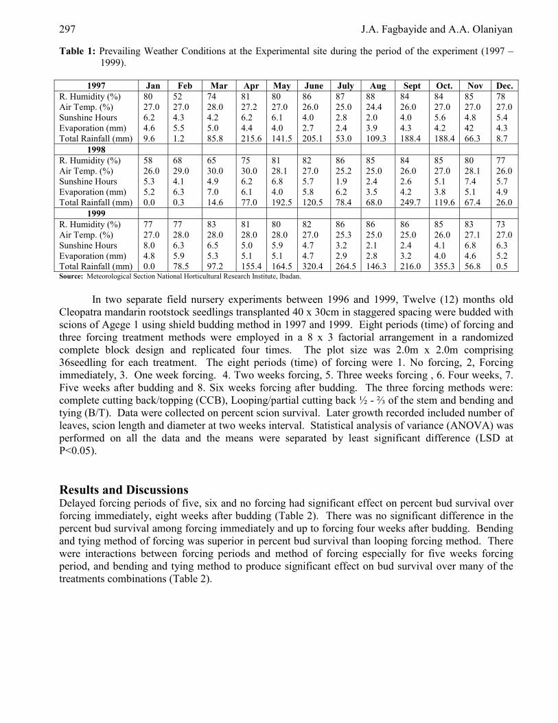
Table 1: Prevailing Weather Conditions at the Experimental site during the period of the experiment (1997 – 1999).

1997 Jan Feb Mar Apr May June July Aug Sept Oct. Nov Dec.

R. Humidity (%) 80 52 74 81 80 86 87 88 84 84 85 78 Air Temp. (%) 27.0 27.0 28.0 27.2 27.0 26.0 25.0 24.4 26.0 27.0 27.0 27.0 Sunshine Hours 6.2 4.3 4.2 6.2 6.1 4.0 2.8 2.0 4.0 5.6 4.8 5.4 Evaporation (mm) 4.6 5.5 5.0 4.4 4.0 2.7 2.4 3.9 4.3 4.2 42 4.3 Total Rainfall (mm) 9.6 1.2 85.8 215.6 141.5 205.1 53.0 109.3 188.4 188.4 66.3 8.7

1998 R. Humidity (%) 58 68 65 75 81 82 86 85 84 85 80 77 Air Temp. (%) 26.0 29.0 30.0 30.0 28.1 27.0 25.2 25.0 26.0 27.0 28.1 26.0 Sunshine Hours 5.3 4.1 4.9 6.2 6.8 5.7 1.9 2.4 2.6 5.1 7.4 5.7 Evaporation (mm) 5.2 6.3 7.0 6.1 4.0 5.8 6.2 3.5 4.2 3.8 5.1 4.9 Total Rainfall (mm) 0.0 0.3 14.6 77.0 192.5 120.5 78.4 68.0 249.7 119.6 67.4 26.0

1999 R. Humidity (%) 77 77 83 81 80 82 86 86 86 85 83 73 Air Temp. (%) 27.0 28.0 28.0 28.0 28.0 27.0 25.3 25.0 25.0 26.0 27.1 27.0 Sunshine Hours 8.0 6.3 6.5 5.0 5.9 4.7 3.2 2.1 2.4 4.1 6.8 6.3 Evaporation (mm) 4.8 5.9 5.3 5.1 5.1 4.7 2.9 2.8 3.2 4.0 4.6 5.2 Total Rainfall (mm) 0.0 78.5 97.2 155.4 164.5 320.4 264.5 146.3 216.0 355.3 56.8 0.5 Source: Meteorological Section National Horticultural Research Institute, Ibadan.

In two separate field nursery experiments between 1996 and 1999, Twelve (12) months old

Cleopatra mandarin rootstock seedlings transplanted 40 x 30cm in staggered spacing were budded with scions of Agege 1 using shield budding method in 1997 and 1999. Eight periods (time) of forcing and three forcing treatment methods were employed in a 8 x 3 factorial arrangement in a randomized complete block design and replicated four times. The plot size was 2.0m x 2.0m comprising 36seedling for each treatment. The eight periods (time) of forcing were 1. No forcing, 2, Forcing immediately, 3. One week forcing. 4. Two weeks forcing, 5. Three weeks forcing , 6. Four weeks, 7. Five weeks after budding and 8. Six weeks forcing after budding. The three forcing methods were: complete cutting back/topping (CCB), Looping/partial cutting back ½ - ⅔ of the stem and bending and tying (B/T). Data were collected on percent scion survival. Later growth recorded included number of leaves, scion length and diameter at two weeks interval. Statistical analysis of variance (ANOVA) was performed on all the data and the means were separated by least significant difference (LSD at P<0.05). Results and Discussions Delayed forcing periods of five, six and no forcing had significant effect on percent bud survival over forcing immediately, eight weeks after budding (Table 2). There was no significant difference in the percent bud survival among forcing immediately and up to forcing four weeks after budding. Bending and tying method of forcing was superior in percent bud survival than looping forcing method. There were interactions between forcing periods and method of forcing especially for five weeks forcing period, and bending and tying method to produce significant effect on bud survival over many of the treatments combinations (Table 2).

Influence of Time and Different Methods of Forcing on Citrus Scion Growth in the Nursery 298

Table 2: Effect of methods and time of forcing on percent (%) bud survival of sweet Orange seedling eight weeks after budding in the nursery

Method of forcing

Time of forcing weeks CCB L B/T Time of forcing means

No forcing 76.20 76.21 72.71 75.04 Forcing immediately 60.96 54.82 67.90 61.23 One week 64.36 60.43 62.31 62.37 Two weeks 59.80 56.00 73.61 63.14 Three weeks 67.10 67.35 77.77 70.74 Four weeks 66.63 68.45 74.40 69.83 Five weeks 73.77 69.32 81.05 74.71 Six weeks 76.16 7.00 77.00 74.39 Methods of forcing means 68.12 65.32 73.43 74.39

Forcing methods Time of forcing Cv% 14.42 18.12 LSD (P=0.05) 6.37 12.78 Forcing methods x time of forcing CV% = 16.22 LSD (P=0.05) = 12.78 CCB = Complete cutting back, L = Looping, BT = Bending and tying.

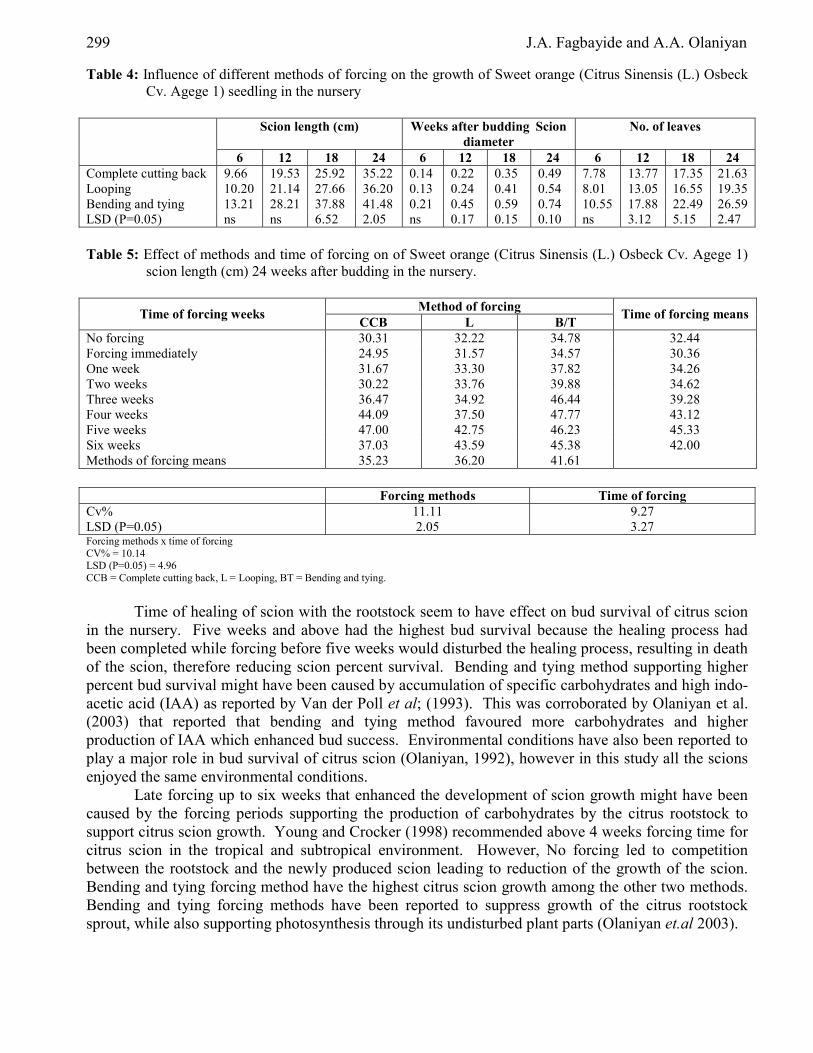
On the scion later growth, scion length was significantly influenced by the time of forcing from twelve weeks after budding (Table 3), late forcing from four weeks after budding improved scion length. Five weeks forcing period stood out though not significantly superior to four and six weeks forcing period. Scion diameter was influenced by time of forcing at twenty-four weeks after budding, there were no significant differences between no forcing, forcing immediately, one and two weeks forcing periods. Forcing time of five weeks enhanced scion diameter, twenty four weeks after budding than any of the above mentioned forcing periods (Table 3). Late forcing also affected number of leaves produced twenty four weeks after budding, three weeks forcing and above were significantly superior influencing leaf production to earlier forcing periods including no forcing also (Table 3). Bending and tying method of forcing influenced growth variables of Agege 1 Sweet orange scion in the nursery. Scion length, scion diameter and number of leaves recorded using Bending and tying method of forcing were significantly superior to looping and topping /cutting back forcing methods (Table 4). Table 5 shows interaction between time of forcing and methods of forcing twenty-four weeks after budding. There were interactions among late forcing periods from three weeks forcing period and the different methods of forcing.

Table 3: Influence of time of forcing on Scion growth of Sweet orange (Citrus sinensis (L) Osbeck. Agege 1)

seedlings in the nursery.

Scion length (cm) Scion diameter No. of leaves Time of forcing 6 12 18 24 6 12 18 24 6 12 18 24

No forcing 6.00 22.09 27.08 32.44 0.18 0.28 0.29 0.40 2.00 10.13 16.34 21.31 Forcing immediately 5.14 18.24 23.51 30.36 0.16 0.25 0.26 0.28 3.17 11.42 17.79 20.19 One week 4.95 22.90 28.48 34.26 0.18 0.23 0.26 0.31 4.08 11.75 20.74 25.20 Two weeks 7.13 22.51 27.74 34.62 0.19 0.28 0.36 0.42 6.01 10.44 22.55 27.30 Three weeks 5.48 24.50 29.50 39.28 0.23 0.28 0.40 0.53 4.62 10.75 26.88 35.70 Four weeks 9.12 28.00 36.62 43.12 0.21 0.27 0.44 0.54 7.81 12.75 24.10 34.70 Five weeks 8.20 32.61 38.32 45.33 0.20 0.27 0.45 0.62 5.75 13.88 26.2 37.70 Six weeks 8.04 30.82 36.61 42.00 0.22 0.28 0.44 0.55 4.04 11.88 24.20 33.80 LSD (P=0.05) ns 5.72 7.31 3.27 ns ns ns 0.18 ns ns ns 6.3

299 J.A. Fagbayide and A.A. Olaniyan

Table 4: Influence of different methods of forcing on the growth of Sweet orange (Citrus Sinensis (L.) Osbeck Cv. Agege 1) seedling in the nursery

Scion length (cm) Weeks after budding Scion

diameter No. of leaves

6 12 18 24 6 12 18 24 6 12 18 24 Complete cutting back 9.66 19.53 25.92 35.22 0.14 0.22 0.35 0.49 7.78 13.77 17.35 21.63 Looping 10.20 21.14 27.66 36.20 0.13 0.24 0.41 0.54 8.01 13.05 16.55 19.35 Bending and tying 13.21 28.21 37.88 41.48 0.21 0.45 0.59 0.74 10.55 17.88 22.49 26.59 LSD (P=0.05) ns ns 6.52 2.05 ns 0.17 0.15 0.10 ns 3.12 5.15 2.47

Table 5: Effect of methods and time of forcing on of Sweet orange (Citrus Sinensis (L.) Osbeck Cv. Agege 1)

scion length (cm) 24 weeks after budding in the nursery.

Method of forcing Time of forcing weeks CCB L B/T Time of forcing means

No forcing 30.31 32.22 34.78 32.44 Forcing immediately 24.95 31.57 34.57 30.36 One week 31.67 33.30 37.82 34.26 Two weeks 30.22 33.76 39.88 34.62 Three weeks 36.47 34.92 46.44 39.28 Four weeks 44.09 37.50 47.77 43.12 Five weeks 47.00 42.75 46.23 45.33 Six weeks 37.03 43.59 45.38 42.00 Methods of forcing means 35.23 36.20 41.61

Forcing methods Time of forcing Cv% 11.11 9.27 LSD (P=0.05) 2.05 3.27 Forcing methods x time of forcing CV% = 10.14 LSD (P=0.05) = 4.96 CCB = Complete cutting back, L = Looping, BT = Bending and tying.

Time of healing of scion with the rootstock seem to have effect on bud survival of citrus scion

in the nursery. Five weeks and above had the highest bud survival because the healing process had been completed while forcing before five weeks would disturbed the healing process, resulting in death of the scion, therefore reducing scion percent survival. Bending and tying method supporting higher percent bud survival might have been caused by accumulation of specific carbohydrates and high indo-acetic acid (IAA) as reported by Van der Poll et al; (1993). This was corroborated by Olaniyan et al. (2003) that reported that bending and tying method favoured more carbohydrates and higher production of IAA which enhanced bud success. Environmental conditions have also been reported to play a major role in bud survival of citrus scion (Olaniyan, 1992), however in this study all the scions enjoyed the same environmental conditions.

Late forcing up to six weeks that enhanced the development of scion growth might have been caused by the forcing periods supporting the production of carbohydrates by the citrus rootstock to support citrus scion growth. Young and Crocker (1998) recommended above 4 weeks forcing time for citrus scion in the tropical and subtropical environment. However, No forcing led to competition between the rootstock and the newly produced scion leading to reduction of the growth of the scion. Bending and tying forcing method have the highest citrus scion growth among the other two methods. Bending and tying forcing methods have been reported to suppress growth of the citrus rootstock sprout, while also supporting photosynthesis through its undisturbed plant parts (Olaniyan et.al 2003).

Influence of Time and Different Methods of Forcing on Citrus Scion Growth in the Nursery 300

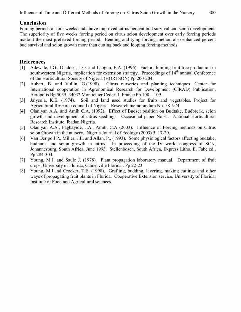
Conclusion Forcing periods of four weeks and above improved citrus percent bud survival and scion development. The superiority of five weeks forcing period on citrus scion development over early forcing periods made it the most preferred forcing period. Bending and tying forcing method also enhanced percent bud survival and scion growth more than cutting back and looping forcing methods. References [1] Adewale, J.G., Oladosu, L.O. and Laogun, E.A. (1996). Factors limiting fruit tree production in

southwestern Nigeria, implication for extension strategy. Proceedings of 14th annual Conference of the Horticultural Society of Nigeria (HORTSON) Pp 200-204.

[2] Aubert, B. and Vullin, G.(1998). Citrus nurseries and planting techniques. Center for International cooperation in Agronomical Research for Development (CIRAD) Publication. Acropolis Bp 5035, 34032 Montieuier Cedex 1, France Pp 108 – 109.

[3] Jaiyeola, K.E. (1974). Soil and land used studies for fruits and vegetables. Project for Agricultural Research council of Nigeria. Research memorandum No. 581974.

[4] Olaniyan A.A. and Amih C.A. (1992). Effect of Budset position on Budtake, Budbreak, scion growth and development of citrus seedlings. Occasional paper No.31. National Horticultural Research Institute, Ibadan Nigeria.

[5] Olaniyan A.A., Fagbayide, J.A., Amih, C.A (2003). Influence of Forcing methods on Citrus scion Growth in the nursery. Nigeria Journal of Ecology (2003) 5: 17-20.

[6] Van Der poll P., Miller, J.E. and Allan, P., (1993). Some physiological factors affecting budtake, budburst and scion growth in citrus. In proceeding of the IV world congress of SCN, Johannesburg, South Africa, June 1993. Stellenbosch, South Africa, Express Litho, E. Fabe ed., Pp 284-304.

[7] Young, M.J. and Saule J. (1978). Plant propagation laboratory manual. Department of fruit crops, University of Florida, Gainesville Florida . Pp 22-23

[8] Young, M.J.and Crocker, T.E. (1998). Grafting, budding, layering, making cuttings and other ways of propagating fruit plants in Florida. Cooperative Extension service, University of Florida, Institute of Food and Agricultural sciences.

European Journal of Scientific Research ISSN 1450-216X Vol.15 No.3 (2006), pp. 301-307 © EuroJournals Publishing, Inc. 2006 http://www.eurojournals.com/ejsr.htm

Impact of Working Capital Management on the Pofitability of

Oil and Gas Sector of Pakistan

S.M.Amir Shah Lecturer, Accounting& Finance

AIOU, PhD Student Muhammad Ali Jinnah University, Islamabad

Aisha Sana Aisha Sana, M. Com, University of Central Punjab, Lahore

Abstract

Working capital in an important component of financial management, this study investigates a relationship between working capital and the profitability of listed companies of Oil and Gas sector of Pakistan for the period 2001-2005. We can analyze working capital management through working capital ratios. Working capital ratios are stock or inventory turnover, receivables ratio, payables ratio, current ratio, quick ratio, and cash conversion cycle. Cash conversion cycle is one of the important measuring tools to calculate the efficiency of working capital. Working capital some times called gross working capital means current assets towards business operations. Net working capital is the current assets less current liabilities. Applying correlation and OLS method using Fixed Effect Estimation model, results show a negative relationship between gross profit marigin and number of day’s inventory and number of day’s accounts receivable, cash conversion cycle and sales growth. Where as there is positive relation between gross profit margin and the number of day’s accounts payables. Results show the existence of firm effect. The analysis also suggest that managers can generate positive returns for the shareholders by managing the working capital. This indicates that working capital management practices adequately explain changes in profitability of the firm.

1. Introduction Working capital of any firm shows the position of liquid assets it holds to build its business. Working capital sometimes called gross working capital simply refers to current assets used in operations. Networking capital is current assets minus current liabilities. Net working capital shows the success of the business operations where as negative working capital shows lack of funds, which are necessary for growth. Every business needs sufficient liquid assets to meet its day-to-day requirements. It needs enough cash o pay wages and salaries as they fall due and to pay creditors if it is to keep its work force and ensure its supplies. To manage working capital is not only sufficient or short-term but also important for the survival of the business in long run. Even a profitable business may fail if it does not have adequate cash flow to meet its liabilities as they fall through. There are three approaches or financing policies (a) Hedging Approach, (b) Conservative Approach, (c) Aggressive Approach. There are basically five most common sources of short-term working capital financing, trade creditors, equity, factoring, line of credit, and short-term loan. Flow of cash in a cycle, inside and outside the business, becomes lifeblood of every business. If a business is operating profitably, then it should generate more or surplus cash. If it doesn't generate surpluses, the business will eventually run out of

Impact of Working Capital Management on the Pofitability of Oil and Gas Sector of Pakistan 302

cash and near to expire. The above discussion highlight the importance of managing working capital for firms in emerging markets with less developed financial and capital markets for countries like Pakistan. It is important to analyze the situation as to how the companies manage their working capital and find out a relationship between firm’s profitability and the working capital management. There are certain measures, which help us to calculate working capital like, Inventory turnover ratio, Accounts receivable ratio, Account payable ratio, Current ratio, quick ratio, Working capital ratio. Section (1) of this research paper contains the literature review on working capital management, section (2) contains explanation of variables and methodology, the last section (3) contains empirical analysis and last section contains conclusion of this research. 2. Literature Review Marc Deloof(2001) carried out research on “intragroup relations and the determinants of corporate liquid reserves”. According to the theoretical world in perfect capital markets, liquid reserves do not matter. A firm will always be able to obtain the necessary funds at zero cost. On the other hand the real or practical world is opposite that means “imperfect”, and some of these “imperfections” lead to costs, which a firm can avoid by holding liquid reserves.

Marc Deloof(2003) carried out research based on Belgian firms in article named “Does working capital management affect profitability of Belgian firms?” This research investigates a relation between working capital management and the profitability of firms. A significant negative relation found between gross operating income and the number of days accounts receivables inventories and accounts payables for a large number of a sample of Belgian firms.

Dev Strischek (2001) discusses that lending bankers judge a company’s working and cash flow management skills, which certainly impact the cost of capital. This is why a lender has a vested interest in three key areas namely; sound collection practices, inventory controls and trade credit disciplines.

Hyun-Han Shin and Luc Soenen (1998) carried out research on a large sample of listed American firms for the 1975-94 periods titled “Efficiency of Working Capital Management and Corporate Profitability”. Stated efficient working capital management is an important part of the overall corporate strategy to create shareholder value and the profitability of firms. Results show a strong negative relation between the cash conversion cycle and corporate profitability

Carol Howarth , Paul Westhead(2003) discussed the working capital management routines of a large random sample of small companies in the UK. Considerable variability in the take up of 11 working capital management routines was detected. Principal components analysis and cluster analysis confirm the identification of four distinct types of companies with regard to pattern of WCM. The first three types of companies focus upon cash management, stock or debtor’s routines respectively, while the fourth types was less likely to take up any WCM routines. Influences on the amount and focus of working capital management were discussed. Regression analysis suggests that the selected independent variables successfully discriminated between the four types of companies. The results suggest that small companies focus only on areas of working capital management where they expect to improve marginal return.

Khan Safi Ullah, Shah Amir and Hijazi Syed conducted a research based on listed Pakistani companies, named “impact of working capital management on the profitability of firms”. This study analyzes the effect of working capital on the profitability of firms and investigates a relation between working capital management and the corporate profitability of the non-financial firms. For this research they took sample size of 30 firms. There results showed a significant negative relationship between firm’s gross profit and the number of days inventories, accounts payable and cash conversion cycle.

C.R.Sathyamoorthi (2000) conducted a research on management of working capital in cooperatives in Botswana. The paper focused on how the current assets components on the basis of

303 S.M.Amir Shah and Aisha Sana

four years data of some selected organizations. The study covered the period of 1994-97. The study showed that the cooperatives had how liquidity resulting their weak position to pay short-term debts.

Ananth Raman Bowon Kim (2001) models the impact of inventory holding cost and reactive capacity on Northco’s targeted under stocking and overstocking cost and offers a solution methodology for such problems. Quantifying the impact of varying inventory-carrying cost on stock out cost and the value of additional capacity, their results illustrate that manufacturers with high working capital cost, and hence high inventory carrying costs, should target higher stock out cost and achieve lower capacity utilization. 3. Methodology In this Research, we examined the relationship between working capital management and the profitability of Pakistan’s Oil and Gas Exploration Sector Companies. There are eleven companies in this sector listed on Karachi stock exchange, out of witch complete data for seven companies from the year 2001-2005 was available. Rest of the four companies for which incomplete data was available, were excluded from the sample. Ratios for working capital items were calculated like number of days accounts receivables, number of day’s inventory turnover and number of day’s accounts payables. The cash conversion cycle is one of the important measures of working capital management. Then Statistical tests, correlation analysis, OLS using fixed effect estimation model were applied. Sources of Data Items relate to the working capital, taken from the annual reports of the companies from 2001-2005. Variables Which help to measure profitability of companies are Gross Profit Margin, which calculated as (Sales - cost of goods sold)/total assets. Number of days accounts receivables defined as (accounts receivable * 365)/sales. Number of days inventories calculated as (inventories*365)/cost of goods sold. Number of days accounts payables is (accounts payable*365)/purchases. The cash conversion cycle is calculated as (number of day’s accounts receivable + number of day’s inventory –number of days accounts payable). Sales growth is (current year’s sale – previous year’s sales)/previous year’s sales.

Impact of Working Capital Management on the Pofitability of Oil and Gas Sector of Pakistan 304

Variables

Years G.P Margin No. of Day Rec.

No. of Day inv

No. of days payables

CCC Goss OP. Margin

Sales Growth

2001 0.358 14.708 26.255 73.881 32.918 0.024 0.461 2002 0.558 20.121 25.686 108.145 -62.338 0.07 0.0776 2003 0.0615 28.93 25.591 100.856 -46.345 0.029 0.13 2004 0.0754 46.79 32.57 130.968 -51.608 0.034 0.086 2005 0.1315 38.405 24.597 121.63 -58.628 0.06 0.637 2001 0.439 74.47 35.06 204.54 -95.01 0.0571 -0.0975 2002 0.488 30.131 23.699 60.461 -6.631 0.046 0.086 2003 0.569 29.436 28.388 54.128 2.872 0.04 -0.018 2004 0.549 23.34 33.035 71.925 -15.54 0.031 0.0947 2005 0.476 33.893 26.422 36.627 23.68 0.018 -0.04 2001 0.079 107.07 38.4 131.57 13.43 0.034 0.158 2002 0.106 56.442 25.462 15.064 -73.16 0.038 -0.064 2003 0.164 67.883 28.561 58.25 38.194 0.043 0.12 2004 0.175 76.501 4.233 93.597 -12.863 0.053 0.911 2005 0.208 22.972 25.177 60.886 -12.737 0.052 0.503 2001 0.031 65.07 24.88 74.827 15.123 0.018 0.22 2002 0.055 32.576 33.698 60.341 5.933 0.007 -0.165 2003 0.292 26.71 5.098 25.96 5.848 0.045 0.348 2004 0.221 31.401 23.482 87.57 -32.687 0.04 0.021 2005 0.383 33.01 19.96 69.03 -14.06 0.059 0.55 2001 0.037 35.58 19.707 43.26 12.027 0.019 0.256 2002 0.044 34.118 20.911 43.97 11.059 0.029 -0.097 2003 0.051 26.95 18.787 56.24 -10.503 0.035 0.126 2004 0.056 29.872 36.324 54.061 12.135 0.045 0.315 2005 0.064 29.46 38.039 60.132 7.367 0.039 -0.063 2001 0.269 100.13 9.238 136.92 -27.552 0.142 0.23 2002 0.296 96.19 9.23 118.52 -13.1 0.157 0.15 2003 0.289 71.69 8.071 99.2 -19.439 0.125 0.072 2004 0.204 58.561 6.071 89.878 -25.246 0.046 0.408 2005 0.187 63.44 5.421 101.04 -32.179 0.054 0.317 2001 0.186 132.65 17.56 10.9 139.21 0.08 0.267 2002 0.2 104.885 14.6 10.54 108.945 0.07 0.267 2003 0.224 14.86 11.477 8.877 17.46 0.065 0.12 2004 0.191 75.27 9.359 69.801 14.82 0.032 0.309 2005 0.156 86.21 9.01 10.84 84.38 0.04 0.148

Empirical Analysis and Results Table no. 1 shows descriptive statistics. The average Gross profit margin is 22.4% of total assets, where as median is 19.1%. Cash conversion cycle is on average of -1.835 days and median is -6.631. The average number of days accounts payables 72.983 days, while median is 69.03 days. Where as the average number of days accounts receivables is 51.99 days and median is 35.58 days. Gross operating profit margin is on average of 5.0% and median is 4.3%. The average sales growth is 19.5% and median is 14.8%.

Empirical evidence from the principal component analysis indicated that smallholders’ farm forestry is an investment with multi-objectives, primarily focussing on monetary and other economic objectives. This finding has significant implications on agricultural technology adoption in general, and tree farming in particular. Thus, it is likewise important to know the farmers’ characteristics and conditions that would likely influence tree growing potential goals and objectives.

305 S.M.Amir Shah and Aisha Sana

Descriptive Statistics Table 1 Results Mean Standard.

Deviation Maximum Minimum Median

Gross Profit margin 0.224 0.162 0.569 0.031 0.191 No. of Days Accounts Receivables 51.992 30.655 132.65 14.708 35.58 No. of Days inventories 21.258 10.329 38.4 4.233 23.699 No. of days Accounts Payables 72.983 43.13 204.54 8.877 69.03 Cash Conversion Cycle -1.835 46.752 139.21 -95.01 -6.631 Sales Growth 0.195 0.228 0.911 -0.165 0.148

Correlation Analysis Table No. 2 shows the correlation among variables. When we see the correlation between gross profit margin (1) and No. of days accounts receivable (-0.176), there is negative relation between them, means when No. of days accounts receivable decreases the profit increases because when a firm receives money it may invest the money in some other projects which increase the profit of the firm. When we examine the correlation between gross profit margin and No. of day’s inventories (-0.006) is also negative relationship, means when the inventory takes more days to be converted into cost of goods sold, profit decreases and vise versa. Cash conversion cycle show negative relationship with profitability, means that wider the cash conversion cycle the firm will have to arrange finance for more number of days hence pay interest which becomes the source of reduction in profit. Sales growth show a negative relationship with profitability which apparently show abnormal results but it does not seem abnormal in Oil and Gas Sector as its demand is more than supply, for more sales the company has to invest a lot initially which reduces the profit. However, results may be confirmed by conducting research on data for long time period. Whereas there is a positive relation between gross profit margin and number of days accounts payable (0.138), which means that when number of days accounts payable increases the profit also increases, firms may invest that money in somewhere else to generate profit. Correlation Coefficients Table 2 Results Gross

profit No. of days account Rec.

No. of days Inv.

No. of days acc payables

CCC Sales growth

Gross profit margin 1 No. of days acc receivable -0.176 1 No. of days inventories -0.006 -0.313 1 No. of days acc payables 0.138 0.143 0.181 1 CCC -0.146 0.389 -0.169 -0.669 1 Sales growth -0.079 0.103 -0.435 0.0438 0.082 1 Regression Analysis Fixed effect model has been used to capture the firm effect. Results show (i2 is significant at P .001) the existence of firm effect, which is a different management style of the companies and different working capital needs. Regression analysis shows P- values of Independent variables individually are not significant. However, joint effect of all coefficients is significant (F= 5.1 at P 0.0005) which means working capital management effects profitability of the firm. R- squared= 0.7098. The independent variables jointly have strong explanatory power. This indicates that working capital management practices adequately explain changes in profitability of the firm.

Impact of Working Capital Management on the Pofitability of Oil and Gas Sector of Pakistan 306

ititititititiiiiiiit UsghBcccBndpBndiBnrdBDaDaDaDaDaDaaY ++++++++++++= 66554433227766554433221

Table 3 Number of obs = 35 F( 11, 23) = 5. 11 Prob > F = 0.0005 R-squared = 0.7098 Adj R-squared = 0.5710

GPmargin Coef. Std. Err. t P>|t| [95% Conf. Interval]

i1 (dropped) i2 .2909505 .0742488 3.92 0.001 .1373551 .4445458 i3 -.036854 .0890724 -0.41 0.683 -.2211143 .1474064 i4 -.0426322 .0771642 -0.55 0.586 -.2022584 .1169941 i5 -.1853617 .078292 -2.37 0.027 -.3473211 -.0234024 i6 .0335775 .1098526 0.31 0.763 -.1936699 .2608248 i7 -.0290723 .1231351 -0.24 0.815 -.2837967 .2256522 ndr -.0017692 .001239 -1.43 0.167 -.0043321 .0007938 ndi -.0027749 .0036572 -0.76 0.456 -.0103403 .0047905 ndp .0004991 .0010052 0.50 0.624 -.0015802 .0025785 ccc .0007302 .0008858 0.82 0.418 -.0011022 .0025625 sgh .01909 .1187545 0.16 0.874 -.2265724 .2647525 _cons .3327327 .1214373 2.74 0.012 .0815204 .583945

i1-i7 are firm dummies to show the firm effect on working capital management. ndr stands for number of days receivable ndi stands for number of days inventory ndp stands for number of days payable. ccc stands of cash conversion cycle. sgth stands for sales growth Conclusion Working capital management is an integral part of financial management that’s why most of the firms make huge investments in their working capital. The study investigates through correlation analysis and Regression analysis using fixed effect model to analyze the relationship between working capital management and the profitability of oil and Gas sector of Pakistan.

Results show a negative relationship between gross profit marigin and number of day’s inventory and number of day’s accounts receivable cash conversion cycle and sales growth. Where as there is positive relation between gross profit margin and the number of day’s accounts payables. Results also show the existence of firm effect, which is a different management style of the companies and different working capital needs. Regression analysis shows that joint effect of all coefficients is significant which means working capital management effects profitability of the firm. The independent variables jointly have strong explanatory power. This indicates that working capital management practices adequately explain changes in profitability of the firm.

Cash conversion cycle has been found negative. On the surface it would seem that a relatively short cash cycle would be a sign of good management. A firm is quick to collect cash from sales once it pays for purchases. But here the catch is that negative cash conversion cycle is due to pending payments of bills on time. That is why the payment cycle is longer than operating cycle. This measure reflects both operating and financing decisions of the firm. Sales growth show negative correlation with profitability which apparently show abnormal results but it does not seem abnormal in Oil and Gas Sector as its demand is more than supply, for more sales the company has to invest a lot initially which reduces the profit. However, results for sales growth may be confirmed by conducting research on data for long time period.

307 S.M.Amir Shah and Aisha Sana

References [1] Ananth Raman Bowon Kim “Quantifying the impact of inventory holding cost and reactive

capacity on an apparel manufacturer’s profitability” Harvard University, Boston, Massachusetts 02163, USA, October2001.

[2] Carole and Paul Westhead, ”The focus of working capital management in UK small firms; Management Accounting Killington: June 2003. Vol 14 Issue 2, p.94

[3] C.R.Sathyamoorthi, ”Management of working capital in selected co-operatives in Botswana”, Finance India Delhi; Sep 2002; Vol 16,issue 3; ABI/INFOFM Global, P1015.

[4] Dev Strischek (April, 2003), “The impact of working capital investment on the value of a company”. Published by RMA Journal.

[5] Hyun-Han Shin and Luc Soenen (1998), “Efficiency of Working Capital Management and Corporate Profitability”, Journal of Financial Practice and Education, Vol. 8, No. 2, pp.37-45

[6] Khan Safiullah, Shah M Amir and Hijaz Syed (2006), “Impact of Working Capital Management on the Profitability of Firms”; Case of Listed Pakistani Companies. Journal of social sciences, AIOU, Islamabad Vol XIII, PP 41-50

[7] Marc Deloof, (2003), “Does working capital management affect profitability of Belgian firms?” Journal of Business, Finance & Accounting, Vol. 30; Issue (3-4), pp. 573-587.doi: 1111/1468-5957.00008.

[8] Marc Deloof (2001), "Belgian intra-group relations and the determinants of corporate liquid reserves", European Financial Management, Vol. 7, Issue 3, pp. 375-392.

European Journal of Scientific Research ISSN 1450-216X Vol.15 No.3 (2006), pp. 308-313 © EuroJournals Publishing, Inc. 2006 http://www.eurojournals.com/ejsr.htm

Stone Settlements of Tivland, Nigeria

Samuel Oluwole Ogundele Department of Archaeology & Anthropology

University of Ibadan,Ibadan Oyo State,Nigeria

E-mail:oluwoleogundele@yahoo.com

Abstract

This piece of work looks at stone settlements located on the local granitic outcrops that dot Tivland. Oral historical and archaeological findings show that the mode of settlement during the pre-colonial times (at least 500 years ago, based on the limited radiocarbon dates at our disposal) was nucleation. This is opposed to the dispersed settlement system that now exists in the area (in the adjoining plains). These two modes of settlement were a response to changing ecological and social challenges in the region. The identified clusters of houses and cooking structures among other settlement features correspond to the contemporary Tiv compounds. This compound is made of members of an extended polygynous family. These clusters and the living houses on the hill complexes were circular in shape, reflecting their cosmic view that the universe is a round phenomenon. Keywords: Tivland, Nigeria, Stone Settlements, Hills, Oral Traditions, Archaeology.

1. Introduction Tivland in the Middle Benue Valley region of Nigeria offers a great deal of opportunities for developing an understanding and appreciation of how ecology affects human culture with emphasis on settlement behaviour and how the latter also makes some impacts on the former. The region which is dotted by granitic outcrops ranging in height between 350 and 600 metres above sea level is a continuation of the Cameroon highlands (Udo 1982: 20 – 22).

Tivland shares a boundary with the north-western part of Cameroon (see fig. 1). This geographical location also plays a significant role in the early history and migrations of the Tiv. The ancestors of the present-day Tiv entered the Middle Benue Valley of Nigeria from north-western Cameroon. According to oral traditions and the limited written documents, one popular reason for the series of migratory waves of the Tiv in pre-colonial times was land hunger including security (Bohannan 1954: 10 – 12).

Therefore, the numerous stone settlements on hilltops and slopes in the study area are an embodiment of the chequered history, culture and general adaptational behaviour of the Tiv which cannot be separated from contemporary lifeways of the people in a neat way. Tiv stone settlements represent a crossroads of ecological behaviour, technology, architecture and history. The need to properly decode the messages they (stone settlements) contain cannot be over-emphasized in order to develop a fuller understanding of the Tiv essence today (Bohannan 1954: 10 – 15; Ogundele 2004: 20 – 70; Kurita 1993: 188; Stone 1992: 153).

Stone Settlements of Tivland, Nigeria 309

Methodology The Middle Benue Valley/ Cross River Archaeological Project is a long-term and multi-dimensional research of the University of Ibadan, Ibadan, Nigeria. It started in 1975 under the direction of Professor Bassey Andah. I joined this team in 1982 and has continued ever since to conduct research in the region (Andah 1983: 50). My focus is on the settlement history of the Tiv.

The research methods are as follows: oral history and archaeology (Gamble 2001: 15 – 20). Fieldwork exercise embarked upon to-date shows that oral traditions are central to the collection, analysis and interpretation of the Tiv settlement history. The people have well-developed oral traditions, which contain some significant aspects of their history and culture. It (oral history) is an important indigenous knowledge system (Ogundele 2004).

The study area (Tivland) has been divided into two major parts for field operations. They are as follows:

1. North-western Tivland 2. South-eastern Tivland

North-Western Tivland The north-western section is made up of contemporary compounds/ settlements like Tse-Agwa, Tse-Dura, Mbaibon, Tse-Khuhe and Ushongo. The study populations for oral historical work cut across age, sex and social status. It is pertinent to note that the Tiv are a highly egalitarian people. Even with respect to the narration of their settlement history, everybody is free to contribute. As a matter of fact, a very young Tiv boy or girl about the age of fifteen years knows some aspects of the people’s settlement histories, which he/she has learnt or heard from the elders. The target of this method of collecting oral historical data is to have a representative picture, thereby increasing the amount of reliance one can place on oral traditions as a source of history. The other study populations include the following:

1. Compound or settlement heads 2. Priests/ religious leaders 3. Elders – males and females within the age bracket of 50 and 90 years 4. Young adults – males and females between the ages of 18 and 49 years An open method of approach (a minimally structured approach) was used in collecting oral

historical information from the locals. In other words, no tape recorders or questionnaire methods were used. This was to ensure that the people relate to us as freely as possible. Such an approach at least in the context of Tivland reduced suspicions to the barest minimum. At least five elderly members of each of the investigated compounds were interviewed.

This is in addition to the other categories of interviewees. As noted above, the very young Tiv (ranging in age between 15 and 18 years) were not disallowed from taking part in the exercise. The atmosphere was free. Questions raised by me include the following:

1. Where did the ancestors of the present-day Tiv come from or were they in the Middle Benue Valley, all along?

2. If they came from somewhere else, what was the name of the place? 3. When did they move out of the place? 4. Why did they move out? 5. Did they meet some people on getting to Middle Benue Valley? 6. Why did they build stone walls round their hilltop settlements? 7. How were these walls constructed? 8. How high were the walls? Several group photographs were taken with the local people and copies given to them later.

This was an attempt to motivate them and to increase the level of friendship between them and I. Many of the contemporary settlements were revisited many months after the first exercise with a view to cross-checking the information earlier obtained.

310 Samuel Oluwole Ogundele

Archaeological reconnaissance and excavations of the north-western part of Tivland were guided to a large extent, by the available oral historical findings. Some of the local informants took part in surveying the local granitic outcrops or hill complexes where the stone settlements were located.

Reconnaissance work involved climbing up and traversing these hilltops and slopes, which were settled by the ancestors of the present-day Tiv. Two categories of sites were identified as follows:

1. Rockshelters 2. Open settlements I have focused on the latter category because it is closely linked to the available oral traditional

evidence. In addition, it has relics of stone walls. Items of field equipment used for this exercise included prismatic compasses, ranging poles and

tapes. The average elevation of this area (north-western Tivland) is 350 metres above sea level. This exercise has led to the location of such archaeological settlement features and artifacts as stone walls, relics of stone houses, potsherds (broken pieces of pottery) and fragments of iron slag.

Some of the discovered sites have been designated as follows: Tse-Dura open settlements 1,2,3,4 and 5. This is in addition to the Ushongo open settlement

(KAS2). This reconnaissance work was followed up by mapping the hilltop/ slope settlements using the plane-table method. Several household clusters were identified from the sites. Similarly, a lot of fairly dressed stones litter each site. The exercise has enabled us to obtain some knowledge of the archaeological distribution maps of the stone settlements including the relationships to each other. Such a step was helpful in determining where to carry out excavations on each of the mapped stone settlements. The follow-up excavations were in form of test pit (1m by 1m) and quadrant method for some of the circular structures. Excavations were by spit level method (10cm per spit level). This exercise was to enable us to have some glimpses of artifact distributions and their relationships to one another. We are however, not unaware of the difficulties posed by the degree of intensity of research in this locality as well as preservation conditions

(Hodder and Orton 1976: 15 – 20; Mangut 1988: 199 – 240). South-Eastern Tivland The contemporary settlement investigated in this locality include Tse-Gbashanam, Akuji, Usamber, Wombo, Nyiev and Ashiakaa. The study populations for oral history were similar to those from the north-western Tivland. In other words, such groups of Tiv as compound heads, priests/ religious leaders, elders between the ages of 50 and 90 years and young adults (between 18 and 49 years of age) were involved. No tape recorders and questionnaire methods were used, so that suspicions among other fears would not be a hindrance to a free flow of information from the members of the local communities. I was also staying directly in one of the houses given me by the compound head of Tse-Gbashanam.

Such an anthropological method of approach led to my developing interest in Tiv diets among other facets of their culture. More than 8 elders were interviewed in each settlement and this was usually done in a most relaxed or informal way. Group photographs were taken as a method of increasing their level of interest and/or enthusiasm about my research in their locality. The settlements were revisited after one year for the purpose of further work and re-checking of the earlier oral traditional evidence and other related information. The questions raised by me were similar to those in the north-western part of Tivland.

Based on the available oral historical findings, we commenced a reconnaissance survey of the locality. Prominent contemporary settlements in the south-eastern part of Tivland include Nyiev, Jato-Aka and Usamber while the investigated ancient stone settlements located on hilltops and slopes were Binda, Bako and Kpe. These three hill complexes have an average length of 1 kilometre while the average height above sea level is 600 metres. Bako hilltop settlement is about two kilometres south-

Stone Settlements of Tivland, Nigeria 311

east of the Binda hill complex, while the Kpe hill is roughly 800 metres west of the Bako hilltop settlement.

Several local members of these communities within the Turan and Ikurav-Ya clans served as guides/ informants during the reconnaissance surveys. Stone walls, relics of stone houses, tuyeres (broken clay pipes for smelting) and fragments of slag (impurities from iron ore following smelting) were discovered during the reconnaissance. This exercise was followed up by mapping of each settlement site using a plane-table method. These settlement features and/or artifacts were in clusters just like those obtained from the north-western Tivland. So far, only the Binda hilltop settlement has been minimally excavated, using test-pit (1m by 1m) and quadrant methods. Results According to the findings during the oral historical surveys, the ancient Tiv entered the Middle Benue valley from the north-western part of Cameroon. The migrations were in waves involving members of different Tiv clans such as Ukan, Ikurav-Ya, Shitire and Turan. They occupied the local granitic hilltops and slopes for security reasons (see fig. 2). These ancient Tiv people descended to the adjoining plains towards the end of the 19th century when peace began to reign in the region.

The hills in the south-eastern part were higher in elevation than those in the north-west. Settlement relics such as stone walls and houses were better preserved in the former region than the latter because of limited human disturbance since their abandonment. For example, the Binda, Bako and Kpe hill complexes were too rugged and high for the contemporary Tiv to do farming there.

Plane-table mapping of the Binda hills show that the settlement features and/or artifacts were in clusters. These clusters were located inside the four identified stone enclosures. These features were non-random and the stone houses were circular in shape. These boulders or stones for house construction were maximally dressed and used unmortared. Two or three stone arrangements having a rough oval shape and ranging in length between 1 and 1.5 metres were identified in each of the clusters.

3 categories of houses on the basis of their floor diameters have been identified and mapped as follows:

1. Small stone houses (2.70 – 3.15 metres) 2. Medium stone houses (3.20 – 4 metres) 3. Large stone houses (4.50 – 5.50 metres) The medium-sized category is the most predominant. The limited excavations on the Binda hill

complex show that the archaeological deposit was very shallow ranging in depth between 30 and 40 cm. In the north-western part of Tivland, the traditions of settlement history were broadly similar. The hilltops and slopes were occupied by the ancestors of the Tiv on arrival from the north-western section of Cameroon. The local granitic hills were generally dome-shaped and lower in elevation. The slopes were much more gentle and were also larger in number. All these hills and slopes were occupied as evident from the relics of stone walls and houses among other settlement features.

Each of these stone settlements has clusters of houses and possible cooking structures as well as granaries. A lot of the artifacts have been destroyed or displaced as a result of contemporary human activities like farming and hunting. Stones or boulders litter each site. The stones for the construction of living houses and protective walls were used unmortared. Three categories of houses have been identified and mapped on the basis of the floors and their diameters. The picture was similar to what was obtained from south-eastern Tivland.

The archaeological deposits in this locality vary from 40cm to 80cm in depth (see fig. 3). These are much deeper than the excavations in south-eastern Tivland.

312 Samuel Oluwole Ogundele

Discussion The oral historical and archaeological findings obtained from Tivland reveal the inseparable character of the people’s settlements from ecology, level of technology, culture and kinship system. The stone walls surrounding each hilltop settlement in the study area were a reflection of the high level of security-consciousness of the ancient Tiv. These stone walls were constructed by communal efforts as shown by the available oral traditional evidence.

Stones were quarried from the local granitic outcrops and used without mortar (see fig. 4). The lower portions of these constructions – walls and houses were usually made of bigger boulders ranging in diameter between 30 and 35 cm. This technique was to ensure their durability. The defensive and to a lesser degree, demarcatory walls must have ranged in height from 1.5 metres to 2 metres, given the amount of stones littering their surroundings.

The heights of houses were shorter averaging 1.5 metres. These houses according to the available oral traditions had thatched roofs. No direct archaeological evidence was available about the nature of the roofs in the face of preservation problems arising basically from the vagaries of time, erosion and human activities. The round shape of the houses as well as clusters is a reflection of the cosmic view of the Tiv. This world view continues up to now.

The hills in the south-eastern Tivland were not occupied for a long period of time compared to what happened in the north-western part. Indeed, these hills were settled during the most turbulent period of their history. At this time, the need for security from external and internal aggression was very great. Such neighbours as the Junkun and Idoma were waging wars against the Tiv. Similarly, one Tiv clan fought against the other in order to settle on these hills for protection.

Nucleated mode of settlement made it possible for several polygynous families to live together on a given hill complex. The identified clusters show that despite the fact that many Tiv were living on a hill complex, the kinship system still survived. The clusters were representing extended polygynous families. This settlement behaviour represents an important component part of the Tiv essence. It (kinship system) goes on up to now.

The arrangements of stones in an oval shape (ranging in length between 1 and 1.5 metres) on the hills represent burials. However, this tentative inference based on oral traditions and field observations needs to be tested later by archaeological excavations. This would be done as soon as we have the relevant expertise and funds. The tripods of stones located in the settlements were cooking structures or places. This settlement feature was also observed from the ethnographic context among the Tiv (Bohannan 1954: 10 – 12; Ogundele 2004: 25 – 30). Conclusion The ancestors of the contemporary Tiv of the Middle Benue valley region of Nigeria settled on the granitic hill complexes that dot the landscape, on their arrival from the north-western part of Cameroon. This research has benefited enormously from oral history and archaeology. The hill settlements were fortified with stones quarried from the hillsides in order to reduce the menace of internal and external aggression to the barest minimum. The ancient Tiv used these stones unmortared. Their circular houses were also constructed with stones without any mortar. Despite the constraint of space on these hilltops and slopes, clusters that are tantamount to contemporary compounds were identified and mapped. This shows that the Tiv settlement is indeed, a crossroads of such domains as ecology, science, technology, history and culture. Acknowledgements My very sincere gratitude goes to Professor Bassey Andah (of blessed memory) for effectively directing the Middle Benue valley/ Cross River Basin Archaeological and Anthropological Project. I am also greatly indebted to my wife (Jumoke) and children – Toyin, Olumide, Laolu and Sanmi for their unfailing support. My great appreciation goes to Mbakighir Nagu, Matthew Nagu and Gideon, all

Stone Settlements of Tivland, Nigeria 313

of the Tse-Gbashanam compound in south-eastern Tivland, for their warmth and cooperation during the fieldwork. References [1] Andah, B.W. 1983. The Bantu “Homeland” Project: Ethnoarchaeological Investigations in parts

of the Benue Valley Region. West African Journal of Archaeology. Vols. 12/13, pp. 23. [2] Bohannan, P. 1954. Tiv Farm and Settlement.Her Majesty’s Stationery Office, London. [3] Gamble, C. 2001. Archaeology: The Basics. Routledge, London. [4] Hodder, I. and Orton, C. 1976. Spatial Analysis in Archaeology. Cambridge University Press,

Cambridge, pp. 10 – 20. [5] Kurita, K. 1993. An Ecological Study on Land Usage of the Nyakyusa People in southern

Tanzania: Continuity and Changes from the traditional society. African Study Monographs. Vol. 14; No. 4, pp. 188.

[6] Mangut, J. 1998. An Archaeological Investigation of Ron Abandoned Settlements on the Jos Plateau: A Case of Historical Archaeology. In; Wesler, K. ed.; Historical Archaeology in Nigeria. Africa World Press, Trenton, New Jersey, pp. 199 – 230.

[7] Ogundele, S.O. 2004. Rethinking West African Archaeology. John Archers (Publishers) Ltd., Ibadan.

[8] Stone, G. 1992. Social Distance, Spatial Relations and Agricultural Production Among the Kofyar of Namu District, Plateau State, Nigeria. Journal of Anthropological Archaeology. Vol. 11, pp. 153.

[9] Udo, R.K. 1982. The Human Geography of Tropical Africa. Heinemann Educational Books, Ltd., Ibadan, pp. 18.

European Journal of Scientific Research ISSN 1450-216X Vol.15 No.3 (2006), pp. 314-318 © EuroJournals Publishing, Inc. 2006 http://www.eurojournals.com/ejsr.htm

Experimental Protective Effects of Yersinia

Anti -Antibodies in Mice

Owhe-Ureghe, U. B Department of Microbiology, Delta State University

Abraka, Delta State, Nigeria

Agbonlahor D. E Department of Microbiology, Ambrose Alli University

Ekpoma, Edo State Nigeria

Abstract

The experimental protective effect of Yersinia anti-idiotype sera was carried out in mice using standard methods. Results show that 20-50% of a set of mice died when they were injected simultaneously with a suspension of Yersinia species (Y. pseudotuberculosis, Y. enterocolitica (0:3), Y,. enterocolitica (0:8), Y. kristensenii (0:11,23), Y. intermedia (0:52,53) and Y. intermedia-like bacteria (0:52,53)) and colloidal carbon particles (CCP), but when another set of mice immunized with Yersinia anti-idiotype sera, 24hr before being challenged with the respective test organisms and CCP, only 10-20% died. Similarly, only 10% of the mice died when mice previously immunized with Yersinia anti-idiotype sera were challenged with the respective test organisms. The results of this study demonstrate a prophylactic (protective) effect of anti-idiotype sera (anti-antibodies) against Yesinia species infections. Clinical trails on the use of idiotypic network for passive immunization against Yersinia species is therefore recommended. Keywords: Anti-idiotype sera Protective effect Challenged

Introduction When an animal is injected with an immunogen, there is the formation of specific antibody due to the inducing immunogen (Oudin and Michael, 1963; Weir, 1983; Agbonlohor, 1986; Obi and Coker, 1989c; Ndip, 1994; Murray, et al., 1998). An enhancing antibody or a new determinant or antigenic stimulus resulting from the combination of antibody to antigen has been reported by Nemazee and Sato (1982). The antigen – antibody complexes, may initiate the activation of the complement system, and sensitise other components of the immune system, thus resulting in the clearance of the antigen from the body circulation, by lysing the bacterial cells (Fukutome et al., 1980; Obi and Coker, 1989a).

Antibodies that are elicited when an antigen is introduced into the animal body have been generally shown to confer some protective effects against related organism(s). Similarly, antibody, formed when anti-antibody is injected into an animal body, may as well have the potential to confer immunity (protection) in line with the phenomenon of antigen – antibody interaction.

A crucial role has been advanced to antibody in vaccine – induced protection against the development of sepsis and other lethal effects of infection with massive doses of a gram negative bacteria (Pseudomonas aruginosa) (Fukutome et al., 1980). The protective effects of anti-idiotype antibody against C. jejuni and P. shigelloides have been respectively documented by Obi and Coker,

Experimental Protective Effects of Yersinia Anti -Antibodies in Mice 315

(1989a) and Ndip, (1994) in rats. The report of Fujimura et al. (1989) revealed that, though an antibody – independent protection can be induced by introduction of an antigen into an animal body, macrophage activation plays a major role in its expression.

Considering the significant role played by antibodies in the elimination of several bacterial agents from the recticuloendothelial system of animals, (or human) and the prevalence of Yersinia species in our environment (Igumbor et al., 1994), the use of immunological procedures in the prevention of yersiniosis in addition to oral rehydration therapy (ORT) and antibiotics in the management of these diseases is important.

The report of this study is on the successful protection of mice from experimental Yersinia species infection using Yersinia anti-idiotype obtained from rabbits immunised with a locally produced idiotype raised against local strains of Yersinia species. Materials and Methods Animals and Bacterial Strains

The mice used in this study (10.6 to 14.2g in weight) were obtained from the Animal HOUSE of college of Medicine, University of Lagos, and were quarantined for two weeks before use. The Yersinia species. used for this study were obtained from Prof. D. E. Agbonlahor’s Laboratory, Department of Microbiology, Ambrose Alli University Ekpoma, Nigeria. These include; Yesrsinia pseudotuberculosis, Y. enterocolitica (0:3), Y. enterocolitica (0:8), Y. krestensenii (0:11,23), Y. intermedia (0:52,53) and Y. intermedia-like bacteria, (0:52,53). All the Yersinia species were resuscitated and re-characterized to confirm their identity. The criteria previously used by Agbonlahor, et al., (1983); and Agbonlahor, (1986) and adopted by Owhe-Ureghe et al, (2002) were employed. These involved testing for Gram reactions, motility (at 250C and 370C), auto-agglutination, sugar fermentation, urease production, citrate utilization, oxidase reaction and invasive property (Sereny,1955; Agbonlahor et al; 1983; Cowan, 1985; Agbonlahor, 1986). Production of Yersinia Anti-Antisera

The Yersinia anti-antibody sera were produced and their titre level determined as previously reported (Owhe-Ureghe, 1999; Owhe-Ureghe, et al., 2002). Briefly; the Yersinia species were grown an macChonkey agar plates for 18-48hrs and were harvested into 10-12ml sterile PBS (pH 7.4) each and washed thrice in PBS. The washed cells were heat killed in water bath for 1hrs, and re-washed thrice in sterile PBS. These were re-suspended in PBS to yield a cell count of approximately 1.0 x 109 cell/ml. After pre-immune bleeding, the rabbits were injected intravenously with increasing doses (0.5 1.0 1.5 and 2.0ml) of Yersinia species antigen at 4 – 7 days intervals for 4 weeks. The antisera which were obtained from the above experiment were injected into the rabbits to produce Yersinai anti-antisera. The rabbits were bled 10 days after the last injection and the sera separated to obtain Yersinia anti-antibody. These were stored at 40C in 1% sodium benzoate. Determination of the specificity and titre levels of the anti-idiotype sera against their specific antigens.

The Yersinia vaccine suspension (50µl) was mixed with equal amount of antisera diluted serially two folds in PBS in microtitre plate and incubated in a water bath at 50oC for 4hr. The initial serum was diluted 1:10 and the end titre was the reciprocal of the highest dilution, showing a partial agglutination with crude antisera diluted 1:5 in PBS. Positive or negative agglutination, was ascertained about 45 seconds after a loop full of bacteria was mixed with a drop (50µl) of antiserum. A loopful of bacteria was mixed with a drop of PBS to test for autoagglutination

316 Owhe-Ureghe, U. B and Agbonlahor D. E

Lethality Test The method of Fujimura et al., (1989) was employed in this study. A group of 300 mice (10 mice per inoculation type) were used for this investigation. In each case, when the various Yersinia species were used, about 1 x 108 CFU/ml was taken for oral inoculation into the mice.

A set of 50 mice were used to test the protective effect of each Yersinia anti-antiserum. The first 10 mice were each inoculated simultaneously with the test organism(s) and 0.4 ml of colloidal carbon particles (CCP); for the second group of 10 mice, they were first inoculated with the Yersinia anti-antiserum, and then inoculated with a mixed inoculum of test organism and 0.4ml of CCP; the third group of 10 mice, were inoculated first with Yersinia anti-antiserum and challenged with the organism 24 hrs later. The forth and fifth sets of mice were inoculated with only CCP and test organism respectively. Result The results obtained as presented on Table 1 below shows that when the various Yersinia species plus the CCP was simultaneously inoculated into the mice, the death rate range from 20% for Y.kristensenii (0:11, 23) to 50% for Y.intermedia-like bacteria (0:52, 53); but when the various test organisms plus the CCP were inoculated into mice previously immunised (24 hrs earlier) with Yersinia anti-antibody, the death rate now ranged from 10% for Y. pseudotuborculosis, Y .enterocolitica, (0:8) Y. kristensenii, (0:11 23), and Y. intermedia-like bacteria (0:52, 53) to 20% for Y. enterocolitica (0:3). For Y. intermedia (0:52, 53) there was diarrhoea production without death. However, when previously immunised mice were challenged with the respective Yersinia species, only Y. enterocolitica (0:3) and Y. intermedia-like bacteria, (0:52, 53) caused the death of mice. Yersinia kristensenii (0:11, 23), and Y. intermedia (0:52, 53); produced mild diarrhoea, while no death were recorded for Y. pseudotuberculosis and Y. enterocolitica, (0:8). Colloidal carbon particle alone did not cause any death, but when a set of mice was injected with the various test organisms, the death recorded ranges from 10% For Y. pseudotuberculosis, Y. enterocolitica (0:8) and Y. kristensenii, (0:11, 23) to 30% for Y. intermedia-like bacteria (0: 52, 53). Table 1: Protective effect of Yersinia anti-antibody in mice.

Mice inoculation Mean number of Death (%). N = 10 a b c d e f

O/CCP 3(30%) 4(40%) 3(30%) 2(20%) 3(30%) 5(50%) O/CCP/A 1(10%) 2(20%) 1(10%) 1(10%) ++ 1(10%) O/A - 1(10%) - + + 1(10%) CCP - - - - - - O 1(10%) 2(20%) 1(10%) 1(10%) 2(20%) 3(30%)

Key: + = MILD DIARRHOEA ++ = SEVERE DIARRHOEA A = YERSINIA PSEUDOTUBERCULOSIS B = Y. ENTEROCOLITICA (0:3) C = Y. ENTEROCOLITICA (0:8) D = Y. KRISTENSENII (0: 11, 23) E = Y. INTERMEDIA (0: 52, 53) F = Y. INTERMEDIA-LIKE BACTERIA (0:52, 53) O/CCP = TEST ORGANISM + COLLOIDAL CARBON PARTICLES (CCP) O/CCP = TEST ORGANISM + CCP/ YERSINIA ANTI-ANTIBODY O/A = TEST ORGANISM + YERSINIA ANTI-ANTIBODY CCP = COLLOIDAL CARBON PARTICLES ONLY O = TEST ORGANISM ONLY

Experimental Protective Effects of Yersinia Anti -Antibodies in Mice 317

Discussion The results of this investigation (Table 1) confirmed earlier report that antibodies (Fukutome et al., 1980, Obi and Coker, 1989a; Ndip, 1994; Jawetz et al., 1998) introduced into an animal or human body could confer some protective effects against related organism(s). A similar phenomenon has been demonstrated in this locality by Ndip (1994) using Plesiomonas anti-antisera.

In this investigation the vaccination of mice with Yersinia anti-antisera conferred some level of protection on the mice. The death rate was reduced to 10% or mild diarrhoea, when the mice were immunised with the Yersinia anti-antisera. This agrees with the results obtained by earlier workers who immunised mice or rat with vaccine preparations of Pseudomonas aeruginosa (Fujimora et al; 1989), Campylobacter jejuni (Obi and Coker 1989a) and Plesiomonas shigelloides (Ndip, 1994).

The results also suggest that the colloidal carbon particle (CCP) impacted or confer some virulence on the Yersinia species or lowered the immune system of the test animals (when the organism and CCP were simultaneously inoculated into the animal) rendering the mice more susceptible to the various Yersina species as suggested by Jones (1971). This is associated with the effect (negative) of CCP on the activity of macrophages (Obi and Coker, 1989b).

The prophylactic (protective) potentials demonstrated by the anti-idotype (anti-anti-bodies) against Yersinia species infections in this investigation is innovative in this Nigeria environment. Clinical trails on the use of idiotypic network for passive immunization against Yersinia species is recommended.

318 Owhe-Ureghe, U. B and Agbonlahor D. E

References [1] Agbonlalor, D.E., T.O. Odugbemi, and O. Dosumu-Ogunbi (1983). Isolation of species of

Yersinia from patients with gastroenteritis in Nigeria J. Med. Microbiol. 16:93-96 [2] Agbonlahor, D.E. (1986). Characteristics of Yersinia intermedia-like bacteria isolated from

patients with diarrhoea in Nigeria. J. Clin. Microbiol. 23(5): 891-896. [3] Cowan S.T. (1985). Manual for the identification of medical bacteria. 3rd Edn. University

press Cambridge 237p. [4] Fujimura, T., T. Suzuki, M. Mitsuyama, H. Soito and K. Nomoto (1989). Antibody-

independent protection against Pseudomonas aeruginosa infection in mice after treatment with a homologous strain vaccine. J. Med. Microbiol. 28: 101-108.

[5] Fukutome, T., M. Mitsuyama, K. Takaya, and K. Nomoto (1980). Importance of antiserum and phagocytic cells in the protection of mice against infection by Klebsiella pneumoniae. J. Gen Microbiol. 119: 225-229.

[6] Igumbor, E. O., D.E. Agbolahor, A. O. Ogbimi, A. O. Ekundayo, J. O. Ike, V. Ekun, F. I. Esumeh and C.L. Obi (1994). Prevalence of Yersiniosis in domestic and wild animal populations of southern Nigeria. J. Med. Lab. Sci. 4:66-70.

[7] Jawetz, E.A., J.L. Melnick, and E.A. Adelberg (1998). Resistance to Antimicrobial Drugs, In: Medical Microbiology. 29th Edn. (G. F. Brooks, J. S. Butel and S. A. Morse, (Eds.) Appleton and Lange, Stanford, Connecticut. Pp. 148 – 150.

[8] Jones, R.J. (1971). Early protection by vaccines in burns. Brit. J. Exp. Pathol. 52: 100-109. [9] Murray, R.P., Rosenthel S.K., Kobayashi; S.G. and A. M. Pfaller, . (1998).Imnmunology, In:

Medical Microbiology. (3rd Ed.) Mosby – Year Book, Inc. St. Lousi, Missouri Pp. 78 – 134. [10] Ndip, R.N. (1994). Immunological Studies on Plesiomonas shigelloides isolated in Nigeria

Ph.D. Thesis, Ambrose Alli University, Ekpoma, Edo State Nigeria. [11] Ndip, R. N.; C.L. Obi; D.E. Agbonlahor; L. N. Ndip; I. B. Enweani and U.B. Owhe-Ureghe

(1999). Serum bactericidal activity against Plesiomonas shigelloides: Role of ABO blood group. J. Sci. Engr. Tech. 6(1): 1556 – 1564.

[12] Nemazee, D.A. and V.L. Sato, (1982). Enhancing antibody: a novel component of the immune response. Pro. Natl. Acad. Sci. USA. 79: 3828-3832.

[13] Obi, C.L. and A.O. Coker, (1989a). Passive protection of rats against Campylobacter jejuni using Campylobacter anti-idiotype. Nig. J. Technol. Res. 1: 99-101.

[14] Obi, C.L., and A.O. Coker, (1989b). Natural bactericidal activity of human serum against strains of Camylobacter jejuni isolated in Lagos, Nigeria. Cent Afr. J. Med. 35: 444-447.

[15] Obi, C.L. and A.O. Coker, (1989c). Diagnostic potential of rabbit Campylobacter anti-antibody. Microbiol. Lett. 42: 145-148.

[16] Oudin, J. and M. Michael, (1963). A new allotype form of rabbit serum myoglobulins apparently associated with antibody function and specificity. Exp. Res. Acad. Sci. (Paris) 257: 805-808.

[17] Owhe-Ureghe U. B. (1999) Immunological and antimicrobial susceptibility studies of local isolates of Yersinia spp. Ph.D Thesis, Ambrose Alli University, Ekpoma, Edo State, Nigeria

[18] Owhe-Ureghe U. B, E. Akpona and J.E. Ideh (2002). Production of Antisera and Anti-idiotype against Yersina spp. Afri. J. Sci. 3(2): 642-655.

[19] Sereny, B. (1955). Experimental shigella keratoconjunctivitis. Acta Microbiol. Acad. Sci. Hung. 2:293-296.

[20] Weir, D. M. (1983). Antigen- antibody reactions. Mod. Trends Immunol. 2: 28-62.

European Journal of Scientific Research ISSN 1450-216X Vol.15 No.3 (2006), pp. 319-326 © EuroJournals Publishing, Inc. 2006 http://www.eurojournals.com/ejsr.htm

Quality Evaluation of Water Sources in Ife North Local

Government Area of Osun State, Nigeria

E. A. Oluyemi Department of Chemistry, Obafemi Awolowo University

Ile-Ife. Nigeria E-mail: Ayodele_oluyemi@yahoo.co.uk

A. S. Adekunle

Department of Chemistry, Obafemi Awolowo University Ile-Ife. Nigeria

W. O. Makinde

Centre for Energy Research and Development, Obafemi Awolowo University Ile-Ife. Nigeria

J. P. Kaisam1

Department of Chemistry, Obafemi Awolowo University Ile-Ife. Nigeria

A. A. Adenuga

Department of Chemistry, Obafemi Awolowo University Ile-Ife. Nigeria

A. A. Oladipo

Centre for Energy Research and Development, Obafemi Awolowo University Ile-Ife. Nigeria

Abstract

The quality examination of water in Ife – North Local Government of Osun State Nigeria was conducted by determining the physico – chemical parameters. Fourty samples including surface water, bore holes, well and pipe borne water were collected from major towns in the Local Government Area and analyzed. Results showed temperature range of 26.5 – 33.0oC, pH (6.526 – 8.905), conductivity (63.0 – 1039.0 S/cm), resistivity (0.00 – 0.02mΩ.cm), salinity (300.0 – 700.0 mg/l), total solids (90.0 – 1175.0 mg/l), total dissolved solids (37.8 – 622.5mg/l), suspended solids (34.5 – 794.0 mg/l),dissolved oxygen (4.483 – 9.483 mg/l), Biological oxygen demand-BOD5 (0.690 – 6.745 mg/l), chloride (3.64 – 184.04 mg/l), Nitrate (1.08 –53.03 mg/l), phosphate (4.99 – 23.07 mg/l) and sulphate (6.02 – 28.95 mg/l). The results obtained agreed with the limits set by both national and international bodies for drinking and domestic water with few exceptions. Pipe borne water was observed to be safest while the surface waters would support aquatic life and recreational activities. Keyword: Path finding, Collision avoidance, behavioural animation, Crowd simulation

Quality Evaluation of Water Sources in Ife North Local Government Area of Osun State, Nigeria 320 Introduction Water is a universal solvent essential to man for various activities such as drinking, cooking, industrial and agricultural processes, waste disposal and human recreation.

The two main problems man contends with are the availability (source and amount) and quality of water (Adeniyi, 2004). In view of its occurrence and distribution pattern, water is rarely easily available to man in the right desirable amount and quality for most of its application. This is no doubt the problem experienced in most cities and towns in the developing nations not to mention their rural settings. These factors had lead to the growing rate of water borne diseases like typhoid fever and Cholera experienced in this part of the world. Even in the developed nation like the United State of America, for the 2- year period (1991 to 1992), cases of outbreaks of diseases associated with contaminated portable water intended for drinking have been reported (Moore et.al.,1993).The outbreak caused an estimated 17464 person to become ill. A large outbreak of cryptosporidiosis in some states in this country in 1993 was attributed to failure in the water treatment system (Edwards, 1993).

Water quality is a term that is most frequently used, but rarely defines probably because it has not a fixed definition, but apparently fairly well understood by users. Thus, the quality of water is a reflection of the source environment and the activities of man, including the use and management measures put in place by him. However, the desirable properties of water quality should among others include the following, viz: adequate amount of dissolved oxygen at all time, a relatively low organic content, pH value near neutrality, moderate temperature, and freedom from excessive amount of infectious agents, toxic substances, mineral matter (Adeniyi 2004).

Sewage discharge is a major component of water pollution, contributing to oxygen demand and nutrient loading to a destabilized aquatic ecosystem (DWAF and WRC, 1995; WRC, 2000). This problem is also serious in areas where wastewater treatment systems are simple and not efficient (Morrison et.al., 2001). Although, it is possible to renovate polluted surface waters to portable standards, this would be both complex and very expensive (Quality of Domestic Water supplies, 1998). This may make water supply unsustainable.

Groundwater is far more protected from pollution than is surface water. It has significantly less self – cleasing ability and is more difficult to treat. Contaminants in surface water can be broken down by exposure to natural oxidants (oxygen and sunlight), or biologically degraded. The rate of chemical reactions is influenced by temperature, which in surface water is variable and can be quite warm. The ground water environment is dark, oxygen – deficient, cool, and supports very limited biological activities so that contaminants may remain quite unchanged over long periods. Howerver, as water percolates through the soil to become part of the ground water, the process of filtration and absorption may significantly improve its quality. Still, water applied for irrigations or as rain to land covered with pesticides or fertilizers can carry nutrients and toxic chemicals into the groundwater unimpeded.

Ife–North Local Government area is one of the fast growing local government area in Osun State, Nigeria in the recent time. The positioning of the Pre – Degree study center run by the authority of Obafemi Awolowo University (O.A.U), Ile – Ife, plus the already existing Federal Government College and the State School of Science are some of the factors for the population upsurge. An investigation through major towns in the local government revealed that the major source of water for most activities is groundwater (well and boreholes), and sometimes streams and rivers most especially in the dry season. These water sources are the alternatives to the epileptic pipe borne water supply, which would have been more reliable source of safe water for the growing population. In the face of this ambiguity, a research was conducted on the different water sources from the major towns in the local government. The towns include: Edunabon, Moro, Yakoyo and Ipetumodu. The results of the analysis are expected to provide information on the quality and the safety of the water, and to serve as a guide in suggesting the best treatment and application the water can be subjected to, in order to produce a good portable water for the communities to supplement the public pipe borne water supply.

321 E. A. Oluyemi, A. S. Adekunle, W. O. Makinde, J. P. Kaisam1, A. A. Adenuga and A. A. Oladipo

Materials and Methods Materials: The polythene containers used for sampling were washed with ions free detergent, rinsed with distilled- deionized water and then pre – treated with 20% nitric acid (HNO3). They were finally rinsed thoroughly with distilled- deionized water followed by drying in the oven to eliminate errors due to metals contamination. Sampling site and Period:

The sampling was carried out in the dry months of March and April, year 2004. The last sampling was carried out in the month of May of the same year for all the towns. The month of May marks the beginning of the raining season in the year after a long dry season characterized with one or two rainfalls. Ten samples (including surface water, well water, bore holes and pipe borne water) were collected from each town using the already treated polythene containers. Methods: The pH, temperature, depth and dissolved oxygen (DO) were determined and recorded immediately at the site. The dissolved oxygen (DO) was determined by using the Winkler’s Method (Ademoroti, 1996). The conductivity, total dissolved solid (TDS), salinity and resistivities were determined in the laboratory using the Jenway conductimeter model MC METTLER TOLEDO. The chloride was determined by argentiometric method, phosphate by Vanadate-molybdate method while sulphate was determined by turbidimetry method and Nitrate (NO3

-) was determined by UV spectrophotometeric method. (American Public Health Association, 1992) The Total Solids (TS), Dissolved Solids (DS), and Suspended Solids (SS) were determined gravimetrically (Ademoroti, 1996). Result and Discussion The results of the analysis of physico–chemical parameters of the water samples from each town are presented in Tables 1- 4. The pH values of the water ranged from about neutral to alkaline (i.e. 6.526 – 8.905). The mean pH values of the water from each town compared with the pipe borne water is presented in Figure 1. The values fall within the range of 6-9 set by World Health Organization (WHO) and the country’s Federal Ministry of Environment (formerly, Federal Environmental Protection Agency, FEPA, 1991). The pH values which give the indication of acidity and alkalinity of the waters show that the surface and ground waters in the area are safe for agricultural, recreational and domestic uses. Table 1: Physico-Chemical Properties of Water Sources from Edun-abon Town

Parameters Minimum Maximun M ean

Coeff of Variance

Pipe-Borne Water

Fed. Min. of Envt. Limit

PH 7.670 8.713 8.01 ±0.32 3.94 7.666 6.5-9.2* Temp(ºC) 26.250 30.500 28.95 ±1.25 0.04 39.000 - DO(mg/l) 5.517 8.104 7.26 ±0.78 0.11 9.483 - BOD(mg/l) 1.035 6.552 3.16 ±1.69 0.52 4.311 - TS(mg/l) 90.000 860.000 404.00 ± 247.62 0.61 140.000 - TDS(mg/l) 42.300 622.500 307.96 ± 202.82 0.66 80.950 - SS(mg/l) 34.500 237.500 96.05 ± 63.59 0.66 59.050 - Conductivity(µS/cm) 70.650 1039.000 498.39 ± 350.10 0.70 133.500 - Resistivity(mΩ) 0.000 0.010 0.003 ± 0.0048 1.61 0.010 - Salinity(mg/l) 300.000 700.000 490.00 ± 119.72 0.24 400.000 - Chloride(mg/l) 12.760 184.040 76.17 ± 66.39 0.87 16.400 200-600 Nitrate(mg/l) 1.900 52.150 32.35 ± 22.26 0.69 1.080 50.100 Sulphate(mg/l) 6.020 27.940 15.66 ± 8.41 0.54 21.020 150 Phospate(mg/l) 5.370 10.510 7.50 ± 1.65 0.22 6.630 - *-- International Maximum Permissible limit

Quality Evaluation of Water Sources in Ife North Local Government Area of Osun State, Nigeria 322

Figure: 1. DO and BOD of Water Samples from the Four towns

Table 2: Physico-chemical Properties of Water Sources From MoroTown. Parameters Minimum Maximum Mean Coeff. Of

Variance Pipe-borne

Water Fed. Min. Of Envt. Limits

PH 7.10 8.028 7.693 ± 0.33 0.04 7.666 6.5-9.2* Temp(ºC) 27.50 32.000 29.950 ±1.40 0.05 29.000 - DO(mg/l) 5.86 9.483 7.197 ± 1.025 0.14 9.483 - BOD(mg/l) 1.035 4.311 2.346 ± 1.06 0.45 4.311 - TS(mg/l) 140.00 525.000 317.50 ±156.23 0.49 140.000 - TDS(mg/l) 37.80 327.000 169.06 ±109.49 0.65 80.950 - SS(mg/l) 55.05 351.700 157.45 ± 87.37 0.56 59.050 - Conductivity (µS/cm) 63.00 728.000 346.68 ±213.68 0.62 133.500 - Resistivity (mΩcm) 0.00 0.020 0.01 ± 0.01 1.42 0.010 - Salinity(mg/l) 300.00 500.000 410.00 ± 73.79 0.18 400.000 - Chloride(mg/l) 3.64 58.310 33.62 ± 17.97 0.54 16.400 200-600 Nitrate(mg/l) 1.08 52.160 27.36 ± 21.33 0.78 1.080 50.100 Sulphate(mg/l) 6.21 28.950 15.55 ± 8.73 0.56 21.020 150 Phosphate (mg/l) 4.99 10.890 7.09 ± 1.62 0.23 6.630 -

Table 3: Physico-chemical Properties of Water Sources From Yakoyo Town.

Table 4: Physico-chemical Properties of Water Sources From Ipetumodu Town.

Parameters Minimum Maximum Mean Coeff. Of Variance

Tap Water Fed. Min. Of Envt. Limits

PH 6.526 8.267 7.57 ±0.68 0.09 7.67 6.5-9.2* Temp(ºC) 29.500 33.00 30.80 ±0.98 0.03 29.00 - DO(mg/l) 5.690 7.414 6.81 ±0.64 0.09 9.483 - BOD(mg/l) 1.035 7.242 2.30 ±1.84 0.08 4.311 - TS(mg/l) 250.000 890.00 517.00 ±216.95 0.42 140.00 - TDS(mg/l) 83.400 773.00 288.9 ±255.25 0.88 80.95 - SS(mg/l) 77.200 607.00 339.66 ±155.29 0.46 59.05 - Conductivity(µS/cm) 136.900 474.50 307.79 ±120.51 0.39 133.50 - Resistivity(mΩcm) 0.000 0.010 0.002 ±0.0042 2.1 0.010 - Salinity(mg/l) 400.000 500.00 435.00 ±47.43 0.11 400.00 - Chloride(mg/l) 18.230 69.75 47.42 ±22.91 0.48 16.40 200-600 Nitrate(mg/l) 4.070 75.23 36.32 ±21.03 0.58 1.080 50.100 Sulphate(mg/l) 6.160 23.61 14.55 ±5.83 0.40 21.02 150 Phosphate (mg/l) 5.620 13.40 8.09 ±2.10 0.26 6.63 -

323 E. A. Oluyemi, A. S. Adekunle, W. O. Makinde, J. P. Kaisam1, A. A. Adenuga and A. A. Oladipo

Parameters Minimum Maximum Mean Coeff. Of Variance

Tap Water Fed. Min. Of Envt. Limits

PH 7.550 8.905 8.16 ±0.38 0.05 7.67 6.5-9.2* Temp(ºC) 30.000 32.500 31.15 ±0.85 0.03 29.00 - DO(mg/l) 4.483 7.414 6.12 ±0.98 0.16 9.48 - BOD(mg/l) 3.104 6.745 5.59 ±1.13 0.20 4.31 - TS(mg/l) 212.500 1175.000 525.70 ±358.71 0.68 140.00 - TDS(mg/l) 83.900 545.000 258.62 ±147.98 0.57 80.95 - SS(mg/l) 84.000 794.000 267.18 ±271.63 1.02 59.05 - Conductivity (µS/cm) 143.000 907.500 430.96 ±245.90 0.57 133.50 - Resistivity (mΩcm) 0.000 0.010 0.002 ±0.0042 2.10 0.010 - Salinity(mg/l) 400.000 600.000 470.00 ±82.33 0.18 400.00 - Chloride(mg/l) 7.290 171.090 77.24 ±50.98 0.66 16.40 200-600 Nitrate(mg/l) 5.110 53.030 38.10 ±18.57 0.49 1.080 50.100 Sulphate(mg/l) 7.440 25.330 14.02 ±5.76 0.41 21.02 150 Phosphate (mg/l) 5.990 23.070 10.45 ±5.43 0.52 6.630 -

The electrical conductivity (EC) of the water ranged between 63.0 and 1039.0µS/cm. Electrical

conductivity of water is a useful and easy indicator of its salinity or total salt content. High salt content in waste effluents can increase the salinity of the receiving water, which may result in adverse ecological effects on aquatic biota (fried, 1991). In this study, it was discovered that the EC of some borehole waters from Edunabon and Ipetumodu (Tables 1 & 4) were quite high (907.5 – 1039 µS/cm) which is likely due to some soluble minerals from the bedrocks. However, they are still less than the European Union recommended limit (2500µS/cm) for potable water.

The salinity values of all the water sources ranged between 300 – 700 mg/l. They are less than the value of 1000 mg/L set by the World Health organization (WHO, 1979). This implies that the water is safe and not polluted. A very high salt concentration (≥1000mg/l) imparts a brackish, salty taste to water and is discouraged because of the potential health hazard. However, salts build-up as a result of waste discharge to the surface water around these towns should be discouraged as it will prevent the water from being reused by the municipalities for domestic and industrial processes such as food preparation, textiles and paper manufacturing and for irrigation in agriculture.

The total solids (90.00—1175.00mg/l) and the total dissolved solids (37.80-622.50mg/l) of the water samples in the area (Figure 2), are below the limit of 1500mg/l for total solids and 500mg/l for total dissolved solids in drinking water (EPA, 1978). Few exceptions are found in boreholes at Edunabon and Ipetumodu where the total dissolve solids are 622.50 and 545.00mg/l respectively. Two well waters near the borehole at Edunabon have dissolve solids 501.00 and 565.50mg/l close to the set standard values. Some treatments may be required to make the waters suitable for domestic purposes.

Quality Evaluation of Water Sources in Ife North Local Government Area of Osun State, Nigeria 324

Figure 2: TS, TDS and Salinity of Water Sources From The Four Towns

The mean concentrations of Chloride, Nitrate, Sulphate and Phosphate for the four towns are

presented in Figure 3. The chloride concentrations ranged between 3.64 and 184.04mg/l. The lowest value in this study was obtained for the surface water at Moro Town. This parameter is an indication that the stream will conveniently support aquatic life with no ecological effect (Fried, 1991). Thus, the surface water could be a major source of aquatic food for the communities in the Local Government Area. Moreover, the water could also be good for domestic purposes bearing in mind that the values are below the recommended standards of 250mg/L by the United State of American Public Health service (Peters and Odeyemi, 1985) and 600mg/l recommended by WHO (1970) for water intended for domestic use.

Figure 3: Chloride,Nitrate, Sulphate and Phosphate of Water Samples from The Four Towns

The nitrate concentrations range from 1.08—53.03mg/l. The high concentration of nitrate in water may give rise to methaenoglobinemia in children bottle-fed with such water. It was reported that the concentration of nitrate above the threshold of 45mg/l is likely to cause methaenoglobinemia while high level of nitrate and phosphates may bring about the problem of euthrophication in reservoirs and streams (Gadd, 1976). Our results showed nitrate content to be high in most of the underground water samples but low in the surface water and the pipe-borne water. The surface water is free of Algae cover as a result of eutrophication, and consequently suffers no depletion in the dissolved oxygen unlike the ground waters. The use of ground water as potable water in this local government could pose serious health problems associated with high nitrate concentration.

The highest phosphate and sulphate values of 23.07mg/l and 28.95mg/l respectively are obtained for the water samples. The phosphate levels are generally high due to blue-green alga growth

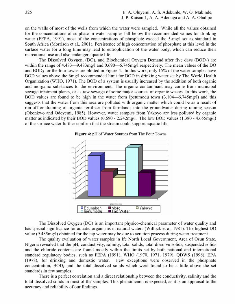
325 E. A. Oluyemi, A. S. Adekunle, W. O. Makinde, J. P. Kaisam1, A. A. Adenuga and A. A. Oladipo

on the walls of most of the wells from which the water were sampled. While all the values obtained for the concentrations of sulphate in water samples fall below the recommended values for drinking water (FEPA, 1991), most of the concentrations of phosphate exceed the 5-mg/l set as standard in South Africa (Morrison et.al., 2001). Persistence of high concentration of phosphate at this level in the surface water for a long time may lead to eutrophication of the water body, which can reduce their recreational use and also endanger aquatic life.

The Dissolved Oxygen, (DO), and Biochemical Oxygen Demand after five days (BOD5) are within the range of 4.483—9.483mg/l and 0.690—6.745mg/l respectively. The mean values of the DO and BOD5 for the four towns are plotted in Figure 4. In this work, only 15% of the water samples have BOD values above the 6mg/l recommended limit for BOD in drinking water set by The World Health Organization (WHO, 1971). The BOD of a system is usually increased by the addition of both organic and inorganic substances to the environment. The organic contaminant may come from municipal sewage treatment plants, or as raw sewage of some major sources of organic wastes. In this work, the BOD values are found to be high in the water from Ipetumodu town (3.104—6.745mg/l) and this suggests that the water from this area are polluted with organic matter which could be as a result of run-off or draining of organic fertilizer from farmlands into the groundwater during raining season (Okonkwo and Odeyemi, 1985). However, water samples from Yakoyo are less polluted by organic matter as indicated by their BOD values (0.690 - 2.242mg/l. The low BOD values (1.380 - 4.655mg/l) of the surface water further confirm that the stream could support aquatic life.

Figure 4: pH of Water Sources from The Four Towns

The Dissolved Oxygen (DO) is an important physico-chemical parameter of water quality and has special significance for aquatic organisms in natural waters (Willock et al, 1981). The highest DO value (9.485mg/l) obtained for the tap water may be due to aeration process during water treatment.

The quality evaluation of water samples in Ife North Local Government, Area of Osun State, Nigeria revealed that the pH, conductivity, salinity, total solids, total dissolve solids, suspended solids and the chloride contents are found mostly within the limits set by both national and international standard regulatory bodies, such as FEPA (1991), WHO (1970, 1971, 1979), QDWS (1998), EPA (1978), for drinking and domestic water. Few exceptions were observed in the phosphate concentration, BOD5 and the total dissolved solids which were found to be a little above the set standards in few samples.

There is a perfect correlation and a direct relationship between the conductivity, salinity and the total dissolved solids in most of the samples. This phenomenon is expected, as it is an appraisal to the accuracy and reliability of our findings.

Quality Evaluation of Water Sources in Ife North Local Government Area of Osun State, Nigeria 326 References [1] Ademoroti, C.M.A. (1996). Environmental Chemistry and Toxicology. Foludex Press Limited,

Ibadan. pp. 44-47. [2] Adeniyi, I.F. (2004). The Concept of Water Quality In: Ife Environmentalist, Official Bulletin

of Nigerian Society for Environmental Management (NISEM) O.A.U., vol.1, No.1, pp 2. [3] American Public Health Association, (1992), Satandard methods for the Examination of Water

and Wastewater, A.E. Greenberg, L.S. Clescert and A. D. Eaton Eds. 18th Edition. Chapter 4, pg 80.

[4] DWAF and WRC (1995), South African Water quality management series. Procedures to assess effluent discharge impacts. WRC Report No TT 64/94. Department of Water Affairs and Forestry & Water Research Commission, Pretoria.

[5] Edwards, D.D. (1993). Trouble waters in Milwaukee. Am. Soc. Microbial News, 59, 342. [6] EPA (1978). Evaluation of the Microbiology Standards for Drinking Water, Environmental

Pollution Agency (EPA), 570/9-78-002, Washington DC, USA. Pp.21-25. [7] Fried J.J. (1991). Nitrates and Their Control in The EEC Aquatic Environment In: Borgadi I.

and Kuzelka D. (eds) Nitrate Contamination, Exposure, Consequences and Control. NATO ASI Series G30, Ecological Sciences, Springer-Verlag, Berlin. 55-63

[8] Gadd, P. (1976), The Ecology of Urbanization and Industrialization. Macmillan Education Ltd. London.

[9] Moore, A.C. et. al., (1993). Surveillance for Waterborne Disease Outbreaks—United States, 1991-1992. In: CDC Surveillance Summaries, MMWR, 42, 55-5, 1.

[10] Morrison G., Fatoki O.S. and Ekberg A. (2001). Assesment of The Impact of Point Source Pollution From The Keiskammahoek Sewage Treatment Plant on The Keiskamma River—pH, Elecrical Conductivity, Oxygen-Demanding Substances (COD) and Nutrients. Water SA., 27: 475-480.

[11] Okonkwo, N. and Odeyemi, O. (1985). Effects of Sewage Lagoon Effluent on The Water Quality of The Receiving Stream, Environmental Pollution (series A), pg 37.

[12] Peters H.I. and Odeyemi O. (1985). Phisico-Chemical Quality of Mokuro Dam in Ile-Ife, Nigeria. Water International, (10),pp. 162-167.

[13] Quality of Domestic Water Supplies (1998). Assesment Guide 1. DWAF, WRC, and Department of Health, Pretoria.

[14] WHO (1970). European Standards for Drinking Water, World Health Organisation, Geneva, Switzerland, Second Edition.

[15] WHO (1971). International Standards for Drinking Water, World Health Organisation, Geneva, Switzerland, Second Edition.

[16] WHO (1979). Sodium Chloride and Conductivity in Drinking Waters. World Health Organization, Copeahagen.

[17] Wilcock R.J., Stevenson, C.D. and Roberts, C.A. (1981). An Inter-laboratory Study of Dissolve Oxygen in Water. Water Research, 15(3): pp. 321-325.

[18] WRC (2000). National Eutrophication of Surface Waters: Policy / Research Needs. Water Research Commission, Pretoria.

European Journal of Scientific Research ISSN 1450-216X Vol.15 No.3 (2006), pp. 327-335 © EuroJournals Publishing, Inc. 2006 http://www.eurojournals.com/ejsr.htm

A Comparative Study of Various Unequal Probability Sampling

Estimators

Hina Muzaffar

M Khalid Pervaiz

M Qaiser Shahbaz

Masood Amjad Khan

Abstract

The performance of Modified Murthy Estimator (MME) of population total developed by Hina and Shahbaz (2004), with various unequal probability sampling estimators, has been compared. For empirical study 20 natural populations from literature on sampling are used. The procedures adopted are relative efficiencies and design effects. The MME showed reduction in the variance of Murthy Estimator (ME) up to 16% and design effect as minimum as zero. Key words: Efficiency, design effect, variance

1. Introduction A lot of work on unequal probability sampling estimator has been done since middle forties. Hansen and Hurwitz (1943) were the first to develop unequal probability sampling estimators.

Midzuno (1952), Sen (1953) extended the Hansen and Hurwitz (1943) scheme, to sampling a combination of n elements from a stratum, with probability proportional to size (PPS) of the combinations. Sen (1953) further generalized the scheme for obtaining an unbiased estimator of the population total when the first r units are selected with PPS. The remaining n-r units are selected with equal probability and without replacement. He has also derived an estimator of the variance estimator. Horvitz and Thomson (1952) presented another technique for selecting n primary sampling units (PSUs) without replacement and with varying probabilities from a finite population. Sen (1954) derived an unbiased variance estimator of an estimator developed by Sen (1953) and showed that this estimate will be always positive. He has also developed a biased estimator for the sample variance, which was more efficient than Horvitz and Thompson’s unbiased variance estimator. Hartley and Rao (1962) derived variance estimator of the population total together with variance estimates for the selection procedure.

Rao (1972) showed that the generalized π ps sampling strategy consisting of the design with πi, the probability of inclusion of the ith unit in the sample, proportional to the modified size together with the corresponding Horvitz-Thompson estimator, is superior to the symmetries. Hanif and Brewer (1979) presented a general theory of sampling with unequal probability, which allowed population units to appear more than once in a sample. They presented two estimators for use in both single stage and multi-stage sampling design. Shahbaz and Hanif (2003a) developed a new estimator of population

A Comparative Study of Various Unequal Probability Sampling Estimators 328

total and obtained design based expectation and variance of the estimator. Shahbaz and Hanif (2003b) developed approximate formulae for the variance of Horvitz-Thompson estimator by using the first order inclusion probabilities. They also checked the validity of the formulae through empirical study. Shahbaz et al (2002) has given a selection procedure with Horvitz-Thompson estimator by merging Brewer (1963) and Durbin (1967) selection procedures.

Hina and Shahbaz (2004) by using the selection procedure of Shahbaz and Hanif (2003), in Murthy (1957), developed an estimator of population total, named as Modified Murthy Estimator (MME) in this study. The objective of this paper is to look at the performance of MME as compared to other estimators available in the literature, with reference to the relative efficiency and design effect. These are described briefly in section 2. 2. Comparison of Different Estimators Numbers of estimators are available in literature for use in unequal probability sampling. Some important estimators compared in this study are described in the following sub sections. 2.1. Hansen – Hurwitz Estimator (HH)

Hansen and Hurwitz (1943) proposed the idea of probability proportional to size sampling with replacement (PPSWR). One unit was selected at each of n draws. They allocate the selection

probability to i-th unit of the population given by ZZ

p ii = where Zi is the measure of size for i-th

population unit and ∑=

=N

iiZZ

1

.

Hansen and Hurwitz proposed the following estimator for population total Y, denoted by HHy′ , for use with unequal probability sampling with replacement:

∑=

=′n

i i

iHH p

yn

y1

1

Where yi is measurement for the i-th unit The variance of this estimator is given by

( ) ⎥⎦

⎤⎢⎣

⎡−=′ ∑

=

N

i i

iHH Y

PY

nyVar

1

21

2.2. Horvitz–Thompson Estimator (HT)

Horvitz and Thompson (1952) were the first to provide a complete theoretical framework for unequal probability sampling without replacement. They suggested the following estimator of population total for use with unequal probability sampling without replacement:

∑∈

=′Si i

iHT

Yyπ

Where Yi measurement for the i-th unit πi probability of i-th unit in sample πij probability of i-th and j-th units in sample Horvitz and Thompson (1952) developed the following variance formula for HTy′ :

329 Hina Muzaffar, M Khalid Pervaiz, M Qaiser Shahbaz and Masood Amjad Khan

( ) ∑∑∑=

≠==

−+

−=′

N

i

N

ijj

jiij

jiiji

N

i i

iHTHT YYYyVar

1 1

2

1

1π

πππππ

2.3. Rao, Hartley, Cochran Estimator (RHC)

Rao – Hartly – Cochran (1962) developed sampling strategy with unequal probability sampling and the estimator of population total.

∑=

=′n

i iT

iTiRHC p

yy1

π

where iTp is the probability of t-th unit selected from the i-th group. Also ∑=

=iN

T iTpi 1π and

11

=∑=

n

i iπ .The of Rao – Hartly – Cochran estimator can be used for any sample size. The variance is

( ) ( )⎥⎥⎥

⎦

⎤

⎢⎢⎢

⎣

⎡∑=

∑=

−−

⎥⎥⎦

⎤

⎢⎢⎣

⎡∑=

−

=′n

i

iN

T nY

iTPiTY

NN

n

iNiNn

RHCyVar1 1

22.

11

2

2.4. Raj Estimator

Raj (1956) proposed the series of ordered estimators that can be used with unequal probability sampling without replacement. The estimator proposed by Raj has the general form as

∑=

=n

rrmean t

nt

1

1

where ∑ ∑−

=

−

=

⎟⎠

⎞⎜⎝

⎛−+=

1

1

1

11

r

i

r

ii

r

rir p

pyyt

The Raj estimator tmean for a sample of size two is:

( ) ( )⎥⎦

⎤⎢⎣

⎡−++= j

i

ii

i

imean p

pyp

pyt 11

21

The variance of the estimator

( ) ( )∑∑=

≠=

⎟⎟⎠

⎞⎜⎜⎝

⎛−−−=

N

i

N

ijj j

j

i

ijijimean

YYpppptVar1 1

2

281

ππ

2.5. Murthy Estimator (ME)

A Modified Murthy Estimator of population total has been developed by using the estimator of Murthy (1957), which is defined as:

( ) ( )∑=

=n

iisymm yiSP

SPt

1)1

where ( )isP is the probability of obtaining a sample “s” given that i-th unit has been already selected and ( )sP is the probability of obtaining a sample “s”. Murthy (1957) used the Yates – Grundy draw – by –draw procedure to obtain following unbiased estimator of population total for a sample of size 2

A Comparative Study of Various Unequal Probability Sampling Estimators 330

( ) ( )

( )ji

ij

jj

i

i

symm pp

ppy

ppy

t−−

⎥⎥⎦

⎤

⎢⎢⎣

⎡−+−

=2

11

2.6. Modified Murthy Estimator (MME):

This estimator is obtaining by Hina and Shahbaz (2004) by using the selection procedure of Shahbaz and Hanif (2003) in Murthy (1957) estimator given in subsection 2.5. The modified Murthy estimator is:

⎥⎥⎦

⎤

⎢⎢⎣

⎡ −+

−−−−−

−−=

j

ij

i

ji

jiji

jimm p

pyp

pypppp

ppbt

)1()1()1)(1)(221(4

)41)(41(

tMM

( )⎥⎥⎦

⎤

⎢⎢⎣

⎡−+= ∑∑

=≠= ji

jiij

j

jij

i

iij

N

i

N

ijj

ijmm PPYY

CPY

BPYADbtV 2

8 2

2

2

2

1 1

where ( )( ) ( )( )

( ) ( )( )bPPPPPPPPPPb

Ajii

iijiijiij 41411

1221441412 −−−

−−−−−−=

( )( ) ( )( )( ) ( )( )jiJ

jjjijiij PPPb

PPPPPPbB

41411*122144141

2 −−−

−−−−−−=

( )( ) ( )( )( )( )( )( )( )jiji

jijijiij PPPPb

PPPPPPbC

414111*1122144141

−−−−

−−−−+−−−=

( )( )ji

jijiij PP

PPPPD

2214141

−−−−

=

3. Empirical Study The estimators described in section-2 are compared by using 20 natural populations from literature on sampling. These are given in Table-A1. For empirical study procedures adopted are relative efficiencies and design effects. 3.1. Relative Efficiency

Relative efficiency of various estimators with respect to MME are obtained and placed in Table-A2. The graph of relative efficiencies for selected twenty populations is given as Figure-1.

The performance of MME with respect to relative efficiency is better as compared to other estimators for the populations 2, 6, 7, 10, 15, 17 and 19. For these populations the relative efficiency of ME ranges from 1.00 to 1.19. It means that the variance of MME may be 84% of variance ME. Thus, the modification introduced by Hina and Shahbaz (2004) reduced the variance of ME up to 16%. It can be considered a reasonable reduction in variance. The MME may produce 21%, 18%, 16%, 17% and 17% smaller variance than HH, HT, HTBDS, RHC, and RAJ estimators, respectively.

331 Hina Muzaffar, M Khalid Pervaiz, M Qaiser Shahbaz and Masood Amjad Khan

3.2. Design Effects

The design effects are computed and placed in Table A3. The graph is given as Figure 2. The design effect of MME is higher than 1 only for populations 3, 12 and 14. For all other

populations the design effect of MME is smaller than 1. It ranges from zero to .88. It implies that variance of MME ranges from extremely smaller to 88% of the variance by simple random sampling. 4. Conclusion The Modified Murthy estimator of population total, proposed by Hina and Shahbaz (2004), has shown:

1. 16% reduction in variance of ME 2. Design effect as small as zero.

A Comparative Study of Various Unequal Probability Sampling Estimators 332

References [1] Brewer, K.R.W. (1963) “A model of systematic sampling with unequal probabilities”,

Aust.J.Stat.5, 5-13. [2] Durbin, J. (1967) “Design of multistage surveys for estimation of sampling

errors:,Appl.Stat.,16,152-164 [3] Hanif, M and Brewer, K. R. W. (1979). Generalization of the Horvitz and Thompson estimator.

Punjab university. J. [4] Math. Vol.12-13, 123-134. [5] Hansen, M. H. and Hurwitz, W. N (1943). On the theory of sampling from finite

population.Ann.Math.Stat.,14.333-362 [6] Hartly, H .O and Rao, J.N, K (1962). Sampling with un equal probability cal. Ann. Maths. stat.

33 [7] Hina,M. and Shahbaz,M.Q.(2004). A Modified Murthy Estimator of population total in unequal

probability sampling. Journal of Statistics Vol 10,No 1,2003. [8] Horvitz, D. G and Thompson, D. J (1952). A generalization of sampling without replacement

from a finite Universe. J.A.SA.,47,663-685 [9] Midzuno, H. (1952). On the sampling system with probability proportional to sums of sizes.

Ibid, 3, 99-107 [10] Murthy, M. N. (1957). Ordered and unordered estimators in sampling without replacement,

Sankhya, 18, 379 – 390. [11] Rao, T. J (1972) Horvitz-Thompson and Des Raj estimators Revisited. The Australian Journal

of statistics, 14. 227-230. [12] Sen A.R (1953). On the estimate of the variance in sampling with varying probabilities”,J.

Ind.Soc.Agri.Stat.,5,119-127. [13] Sen, A. R (1954) on the estimate of variance in sampling with varying probabilities presented at

the 41st session of the Indian science congress hyderabad. [14] Shahbaz, M.Q., Hanif, M. and Samiuddin, M.(2002). On some estimators in unequal

probability sampling. J. Statist. Theory and Appl. Vol. 1(4),239-252,(USA) [15] Shahbaz, M.Q. and Hanif, M. (2003a). Modification of Murthy’s estimator under various

selection procedures for probability sampling without replacement. Pak.J.Statist.Vol. 19(2) 241-250.

[16] Shahbaz, M.Q. and Hanif, M. (2003b). Variance formulas for Horvitz-Thompson estimator using first order inclusion probabilities. J. Applied Statistical Sciences. Vol.(12),201-208(USA).

333 Hina Muzaffar, M Khalid Pervaiz, M Qaiser Shahbaz and Masood Amjad Khan

Appendix

Table-A1: Natural Populations Sr. No. Values of Variables

X 0.3, 0.5, 0 .4, 0.9, 0.7, 0.2, 0.6, 0.5, 0.8, 0.4, 0.8, 0 .6 1 Y 6, 9, 7, 19, 15, 5, 12, 9, 20, 9, 18, 13 X 12, 11.4, 7.9, 9.0, 10.5, 7.9, 7.3, 10.2, 11.7, 11.3, 5.7, 8.0, 10.3, 12.0, 9.2 2 Y 125, 119, 83, 85, 99, 117, 69, 133, 154, 168, 61, 80, 114, 147, 122 X 62, 62, 87, 65, 58, 92, 88, 79, 83, 62, 63, 62, 60, 75, 90 3 Y 2, 3, 3, 5, 4, 7, 2, 4, 2, 5, 3, 6, 4, 4, 2 X 80, 81, 117, 85, 12, 342, 32, 190, 852, 78, 55, 638, 100, 532, 132, 11, 318 4 Y 117, 287, 250, 244, 0, 1806, 64, 328, 4813, 89, 53, 1368, 316, 1035, 256, 9, 471 X 3, 4, 4, 6, 8, 10, 12, 11, 14, 17, 20 5 Y 2, 5, 4, 5, 9, 8, 9, 8, 12, 15, 17 X 104, 106, 106, 106, 102, 104, 102, 104, 102, 102, 101, 105, 106 6 Y 38.9, 40.4, 39.9, 40.8, 33.7, 39.5, 33.0, 39.5, 37.0, 33.9, 29.9, 39.5, 40.6 X 453, 460, 462, 467, 501, 503, 514, 515, 541, 542, 543, 562, 570, 586, 601 7 Y 194, 161, 222, 223, 96, 164, 318, 272, 155, 292, 214, 275, 100, 418, 189 X 7, 3, 5, 8, 12, 4, 6, 11, 8, 9, 5, 7, 6, 11, 5, 5, 7, 17, 12, 10, 10, 6, 5, 8

8 Y 3.2, 1.1, 2.4, 3.7, 6.2, 1.7, 2.1, 3.9, 4.7, 5.1, 2.3, 1.8, 1.6, 3.5, 4.1, 2.4, 6.8, 11.7, 8.3, 5.9, 6.1, 2.3, 7.5, 8.4

X 12, 12, 12, 12, 12, 12, 12, 12, 11, 11, 11, 11, 10, 10, 10, 10 9 Y 762, 651, 461, 521, 653, 544, 542, 590, 533, 517, 520, 539, 509, 449, 492, 498 X 6, 6, 6, 6, 6, 5, 5, 5, 4, 4, 4, 4, 4, 4, 4, 4 10 Y 165, 224, 192, 161, 104, 94, 102, 115, 110, 109, 83, 36, 61, 92, 75, 64 X 94, 85, 85, 80, 82, 79, 86, 82, 93, 88 11 Y 16, 20, 18, 17, 14, 15, 19, 13, 19, 17 X 2, 3, 3, 5, 4, 7, 2, 4, 2, 5, 3, 6, 4, 4, 2, 5, 3, 4, 2, 4

12 Y 14.3, 20.8, 22.7, 30.5, 41.2, 28.2, 24.2, 30.0, 24.2, 44.4, 13.4, 19.8, 29.4, 27.1, 22.2, 37.7, 22.6, 36.0, 20.6, 27.7

X 7, 3, 5, 8, 12, 4, 6, 11, 8, 9, 5, 7 13 Y 3.2, 1.1, 2.4, 3.7, 6.2, 1.7, 2.1, 3.9, 4.7, 5.1, 2.3, 1.8 X 6, 11, 5, 5, 7, 17, 12, 10, 10, 6, 5, 8 14 Y 1.6, 3.5, 4.1, 2.4, 6.8, 11.7, 8.3, 5.9, 6.1, 2.3, 7.5, 8.4 X 7, 6, 3, 3, 8, 5, 5, 7, 9, 1, 3, 4, 6, 4, 7, 6, 4, 3, 7, 5, 5

15 Y 0.82, 3.0, 3.32, 5.0, 7.92, 1.62, 2.66, 4.66, 6.64, 18.0, 0.0, 0.16, 0.50, 4.80, 2.65, 1.95, 2.0, 0.44, 1.98, 3.57

X 8, 10, 7, 5, 12, 4, 10, 6, 7, 5, 11, 3, 7, 8, 11 16 Y 9.2, 15.7, 8.4, 7.5, 18.3, 7.6, 9.5, 9.3, 8.4, 16.5, 20.1, 7.2, 11.6, 9.2, 18.9 X 1, 1, 2, 3, 4, 4, 5, 5, 55, 5, 5, 5, 5, 5, 5, 5, 5, 5, 5 17 Y 21, 23, 40, 43, 50, 96, 145, 156, 127, 161, 214, 143, 201, 198, 173, 220, 297, 151, 158, 163 X 95, 79, 30, 45, 28, 142, 125, 81, 43, 53, 148, 89, 57, 132, 47, 43, 116, 65, 103, 52 18 Y 9, 7, 3, 2, 3, 8, 9, 10, 6, 2, 16, 4, 5, 13, 4, 9, 12, 8, 9, 8 X 51, 51, 52, 52, 53, 54, 57, 60, 65, 67, 68, 70, 71, 73, 74, 76, 78, 80, 81, 85

19 Y 1350, 1176, 1841, 2606, 2656, 2546, 2911, 3280, 3425, 3416, 3390, 3395, 3417, 3290, 3481, 3520, 3570, 330, 520, 3601

X 6.7, 8.2, 7.9, 6.4, 8.3, 7.2, 6.0, 7.4, 8.1, 9.3, 8.2, 6.8, 7.4, 7.5, 8.3, 9.1, 8.6, 7.9, 6.3, 8.9 20 Y 7.1, 8.4, 8.2, 6.9, 8.4, 7.9, 6.5, 7.6, 8.9, 9.9, 9.1, 7.3, 7.8, 8.3, 8.9, 9.6, 8.7, 8.8, 7.0, 9.4

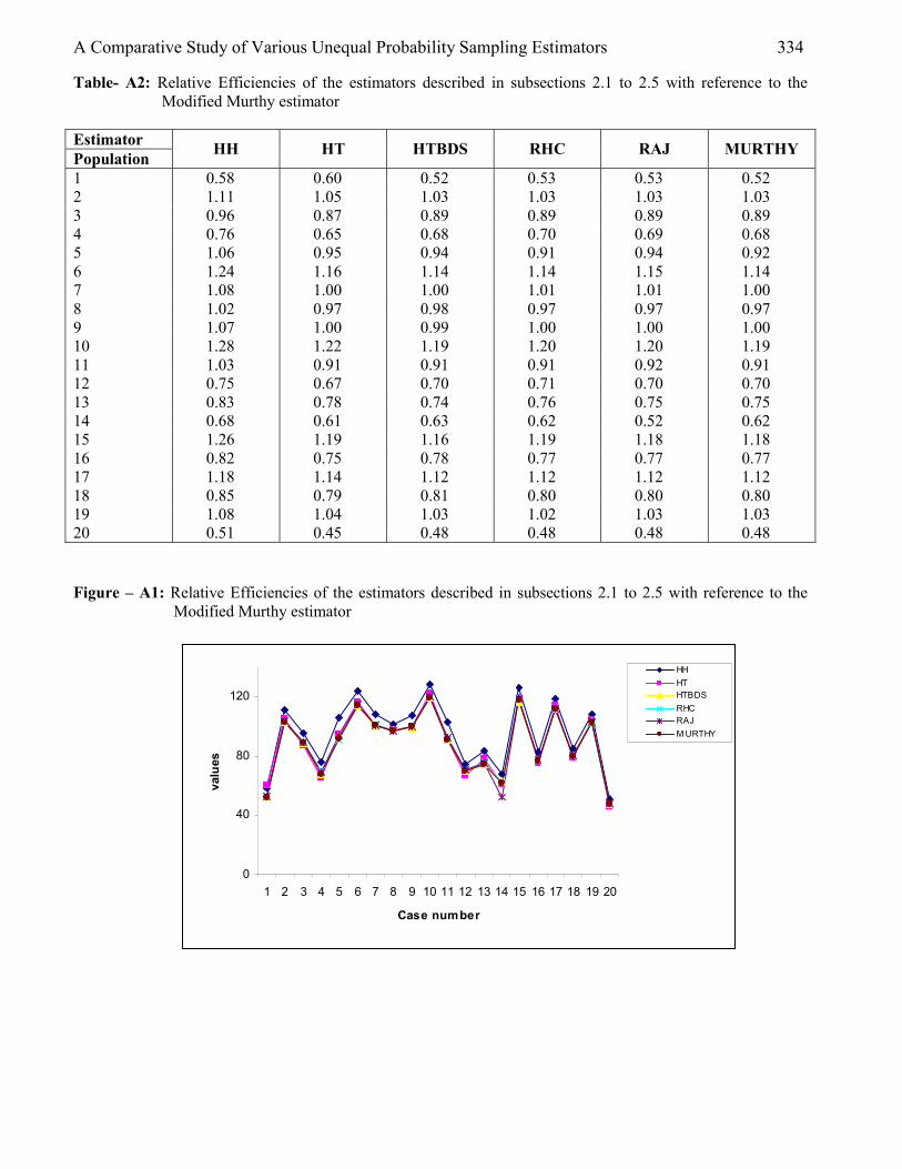
A Comparative Study of Various Unequal Probability Sampling Estimators 334

Table- A2: Relative Efficiencies of the estimators described in subsections 2.1 to 2.5 with reference to the Modified Murthy estimator

Estimator Population HH HT HTBDS RHC RAJ MURTHY

1 0.58 0.60 0.52 0.53 0.53 0.52 2 1.11 1.05 1.03 1.03 1.03 1.03 3 0.96 0.87 0.89 0.89 0.89 0.89 4 0.76 0.65 0.68 0.70 0.69 0.68 5 1.06 0.95 0.94 0.91 0.94 0.92 6 1.24 1.16 1.14 1.14 1.15 1.14 7 1.08 1.00 1.00 1.01 1.01 1.00 8 1.02 0.97 0.98 0.97 0.97 0.97 9 1.07 1.00 0.99 1.00 1.00 1.00 10 1.28 1.22 1.19 1.20 1.20 1.19 11 1.03 0.91 0.91 0.91 0.92 0.91 12 0.75 0.67 0.70 0.71 0.70 0.70 13 0.83 0.78 0.74 0.76 0.75 0.75 14 0.68 0.61 0.63 0.62 0.52 0.62 15 1.26 1.19 1.16 1.19 1.18 1.18 16 0.82 0.75 0.78 0.77 0.77 0.77 17 1.18 1.14 1.12 1.12 1.12 1.12 18 0.85 0.79 0.81 0.80 0.80 0.80 19 1.08 1.04 1.03 1.02 1.03 1.03 20 0.51 0.45 0.48 0.48 0.48 0.48

Figure – A1: Relative Efficiencies of the estimators described in subsections 2.1 to 2.5 with reference to the Modified Murthy estimator

0

40

80

120

1 2 3 4 5 6 7 8 9 10 11 12 13 14 15 16 17 18 19 20

Case number

valu

es

HHHTHTBDSRHCRAJM URTHY

335 Hina Muzaffar, M Khalid Pervaiz, M Qaiser Shahbaz and Masood Amjad Khan

Table- A3: Design Effect of Modified Murthy Estimator of Population Total )ˆ(Y Population No. SRSYVar )ˆ( MMYVar )ˆ( Deff.

1 1612.727 194.5197 0.120615 2 98370.07 31051.92 0.315664 3 229.3571 324.7853 1.416068 4 1.78E+08 2127.426 1.2E-05 5 1062.9 128.5696 0.120961 6 918.94 660.5193 0.718784 7 710508.5 628093.1 0.884005 8 1913.885 849.226 0.443718 9 720850.2 466323.4 0.646907 10 283385.7 111366.2 0.392985 11 211.5556 194.5471 0.919603 12 12149.53 19990.79 1.645397 13 146.6 39.65136 0.270473 14 552.8545 636.8251 1.151885 15 2898.503 1044.86 0.360483 16 2119.576 1872.936 0.883637 17 983823.2 331138.8 0.336584 18 2582.053 1660.952 0.643268 19 2.02E+08 41551304 0.205197 20 164.8942 24.80693 0.150441

Figure – A2 Design Effect of Modified Murthy Estimator of Population Total )ˆ(Y

European Journal of Scientific Research ISSN 1450-216X Vol.15 No.3 (2006), pp. 336-343 © EuroJournals Publishing, Inc. 2006 http://www.eurojournals.com/ejsr.htm

Germination and Seedling Growth as Influenced by Seed Size of

Dacroyodes Edulis (G. Don) H. J. Lam in Nigeria

Ekeke B.A Department of Forestry & Environment

Rivers State University of Science & Technology Port Harcourt, Nigeria

bukkibadef@yahoo.com

Oyebade B.A Department of Forestry & Environment

Rivers State University of Science & Technology Port Harcourt, Nigeria

Adesina, M

Department of Forestry & Environment Rivers State University of Science & Technology

Port Harcourt, Nigeria

Abstract

Dacryodes edulis (G. Don) H. J. Lam was classified into characteristic sizes and evaluated for germination, seedling growth and biomass in six seed size classes. The germination and growth of the seeds were high. The viability and germination of the seeds were between 96-100%. Germination was linearly and positively correlated with seed and fruit weights and lengths. Heavier seeds and fruits showed early and rapid germination. Contribution of fruit dry weight to fresh fruit biomass was 30.90-35.97%. The relative growth rate was high in LB and MB seed size class (0.023-0.026cm/wk) and least in SB seed size class (0.011cm/wk). The study concludes that the variations in fruits and seed size have a significant influence on growth and biomass accumulation in Dacryodes edulis. Such variation manifests in the germination and growth of the species.

Introduction Dacryodes edulis (G. Don) H. J. Lam is an oleiferous fruit tree of the familyBurseracceae, locally known as African Pear. It is an indigenous African tropical forest tree species, which has made transition from the forest to the farm because of the valued fruits.(Awono et al 2002). It is commonly cultivated in agroforestry systems as a shade provider and secondary crop in cocoa and coffee farms (Sonwa et al, 2002). In common with many non-timber forest products (NTFPs), it plays an important role both in household consumption and a source of income (Awono et al, 2002). The nutritional value of the fruit is significant with a fat content of 50%, 27% fibre, 10% protein and 10% sugar (Silou, 1994). Many studies have been carried out on Dacryodes edulis in recent times. Okafor (1983) defined two varieties D. edulis var edulis and D. edulis var. parvicarpa; which was based mainly on fruit size. Some parts of Nigeria (mainly the Ibo speaking areas) in the South-east have identified varieties of the

Germination and Seedling Growth as Influenced by Seed Size of Dacroyodes Edulis (G. Don) H. J. Lam in Nigeria 337

fruit by giving names to different cultivars of the fruit depending on its size, shape, colour, pulp thickness, taste, time of maturity etc. (Okorie 1985). Leakey and Ladipo (1996) reported continuous variation in fruit size, pulp seed ratio and other fruit characteristics between different fruitlots of different origins. Yombi et al (1980) indicated that there are two morphological types in markets in Cameroon: a large fruit with a large seed and a small (short) fruit with a well-developed mesocarp.

Though, the effect of seed size and weight on growth of tree species have been studied by many researchers (Ayuk et al, 1999; Black and Janssens 1996; Bouqest 1969; Dalziel 1937; FAO 1982), there is dearth of information about the relationship of seed traits on seedling growth of dacroyodes edulis. For Dacryodes edulis, which is propagated through seeds, the tree growth correlation with seed is useful for selection of fruits.

The present study was taken up to explore the relationship of fruit and seed size variation on germination and seedling growth of Dacryodes edulis. Materials and Methods Study site

This study was carried out in Port Harcourt, in the Forestry Nursery of University of Science and Technology, Rivers State, situated at the Eastern coast of Nigeria at latitude 4.51o North and longitude 7.01o East on an elevation of 18m above sea level (FAO, 1984). Port Harcourt lies in the humid tropical zone with annual rainfall which ranges from 2000 – 2,470mm, with an annual temperature ranges from minimum 23oC to average maximum 32oC (RISADEP, 1995). Seed procurement

Ripe fruit collection was done in four local markets in Rivers State of Nigeria, which were Obigbo Market, Borokiri Market, Etche market and Oil Mill market. A fruit is ripe when it changes from the unripe pink colour to blue. Questionnaires were administered personally to each D.edulis trader. The fruits were bought from randomly selected traders where the fruits appeared to be similar morphologically confirming common tree origin. Two hundred and forty fruits were randomly selected for identification. The fruit size was initially used for identification and they were Large-Big (LB), Large-Small (LS), Medium-Big (MB), Medium-Small (MS), Small-Big (SB) and Small-Small (SS) (Table1). Thus, six fruit types were identified based on the fruit and seed sizes classification and there were forty of each identified fruit type.

Simple linear correlation and Regression analyses were used to test for association between the fruit lengths and seedling heights, fruit weight and seed weight and for prediction of the fruit type. Fruit and Seed Assessment and Germination

The six identified fruit types were further assessed for fruit weight by weighing with a balance, fruit length and fruit breadth by direct measurement, then fruit shape and colour by visual observation. After these measurements a utility nursery knife was used to open up the fruits to extract the seeds. This was done carefully with the hand in order not to destroy the mesocarp and the seed.

After extraction, the seeds were sown in germination boxes measuring 42cm X 29cm x 8cm and containing river-washed sand and completely decomposed sawdust, in a ratio of 1:2 by volume, respectively in accordance with Okorie and Ezeanyika (2000).

The mesocarp and the endocarp of these seed were previously removed before sowing in the germination media. Each germinaion box contained 10 seeds of a fruit type and there were four replications of each fruit type giving 24 sowing boxes laid out in completely randomized design. These were watered immediately. Watering was also done every morning until the seeds germinated.

338 Ekeke B.A, Oyebade B.A and Adesina, M

Germination counts were taken at intervals of 2 days and germination was deemed successful when the plumule emerged above the soil surface.

The seedlings were transplanted according to the fruit types into polypots measuring 26cm x 19cm x 19cm in size and laid out in completely randomized design. The transplant medium was a mixture of forest topsoil and river sand in a ratio 1:1. Watering was done daily. Total seedling height (cm), and number of leaves were assessed weekly. Biomass was assessed for each fruit type at the end of twelve weeks. The total leaf area and number of roots for each fruit type seedling were also determined. Results and Discussion Fruit Characteristics

The fruit shape varied from oblanceolate and lanceolate, which had the largest length, breadth and weight, found among the Large-Big, Large-small, to obovate which was found among the Medium sizes, then the ovate and elliptic found among the small sizes. The fruit length is highest (7.81cm) in the fruit type L-B (Large-Big) and lowest (3.68cm) in the fruit type S-S (Small –Small). The same trend was observed in the fruit breadth with 3.37cm in L -B and 2.07cm in S-S.

The fruit weight also followed the same sequence. This same trend was observed in the seed length, seed breadth and seed weight (Table 1).

This trend confirms that variations indeed exist in the fruit sizes and the variations also cut across into the seeds, that is, the bigger the fruits, the bigger the seeds or the smaller the fruits, the smaller the seeds. This trend appears to be consistent with fruits of particular parent trees. No morphological variations were observed amongst fruits from the same parent tree. This can help farmers or private individuals in fruits selection for planting, knowing fully well from the market survey, that bigger fruits get bigger sales (prices). (Okorie and Ezeanyika 2000). Table 1: Morphological Characteristics of Dacryodes edulis (G. Don) H. J. Lam

Seed weight classes Parameters LB LS MB MS SB SS Fruit length (cm) Fruit length 7.81a 6.55b 5.66c 4.73d 4.06e 3.68f Fruit breadth 3.37a 3.06b 2.7c 2.5d 2.21e 2.07f Fruit weight 46.13a 40.00b 27.00c 20.00d 16.25e 14.00f Seed length (cm) Seed length 4.75a 4.51b 4.26c 3.65d 3.34e 3.14f Seed breadth 2.47a 2.26b 2.12c 2.03d 1.74e 1.77f Seed weight 15.24a 11.5b 9.5c 7.73d 6.25e 5.60f Leaf attribute Seedling leaves No 4a 3 b 3c 3d 2e 2f Seedling Leaf area (cm2) 29.86a 26.67b 25.66c 23.44d 18.81e 24.57f Root count 21.75a 17.08b 25.75c 16.75d 15.00e 18.5f Relative Growth Rate 0.026a 0.023b 0.025c 0.012d 0.011e 0.014f (RGR – cm)

Seed Germination Commencement of germination among all the fruits types was fourteen days after sowing. Small fruit types however had higher percentage germination than the medium and large fruit types (Table 2 and 3).

Germination and Seedling Growth as Influenced by Seed Size of Dacroyodes Edulis (G. Don) H. J. Lam in Nigeria 339

Figure: 1: Cumulative Germination curve

The cumulative germination rate is shown on Fig.1. The germination rates are also higher in small fruits types. This follows that seeds of the small fruit type (SB and SS) will surely germinate and grow up to seedlings stages that can withstand environmental stress according to Nwoboshi (1982).

Germinative energy or seed vitality therefore follows the same trend (Fig.1). The small fruit type (SB) reached the peak of its germinative energy at week four (4) with 65% germination count while the large fruit type (LB) at week four (4) had about 28% germination count. This suggests that the seed of the small fruit type may have greater capacity to thrive even in adverse environmental conditions than the Large or Medium fruit types. Oni and Gbadamosi (1998) reported that the rate of germination and percentage germination of seeds are important factors in nursery and field establishment of forest crops.

This same trend was observed in the germinative capacity or seed viability. The highest recorded seed viability was found among the small fruit type with 100% germination count (Table 3). This also confirms that the seed of the small fruit type has the potential to withstand more environmental stress and can have a higher yield than the seed of the large fruit type. The results suggest that trees of smaller seed types may be reliable as environmental management trees for shade and erosion control. Ability to germinate early and grow may be a genetic quality for survival in adverse environmental conditions. Selection for environmental management functions may consider small seed/fruit types as a planting option. Seedling growth Height: Table 2 shows the variation in the shoot height of various fruit seed sizes. At the 84 DAS, the lowest height was observed in SB and SS (25.44cm and 24.65cm respectively) while LB fruit type had the highest shoot height at the 84 DAS (LB 32.85cm, LS 31.72cm). There was also significant and positive linear relationship between seedling height and fruit length, (R2 =0.981), and between seedling height and seed length (R2 = 0.934) as shown in (Fig.2). This indicates that fruit and seed lengths affect the seedling height, that is small fruits or seeds tend to grow slower than large fruits or seeds. This also can be a guide to farmers in choosing the type of fruits to plant, since fruits and seeds with higher length will give seedlings with higher height and faster growth rate.

340 Ekeke B.A, Oyebade B.A and Adesina, M

Table 2: Germination and Shoot growth in different Seed size classes of Dacryodes edulis (G. Don) H. J. Lam

Seed weight classes Time (day) LB LS MB MS SB SS Germination % 14 DAS 2.5a 13.3a 10a 2.5a 37.5a 23.3a 28DAS 1.5b 40b 50b 42.5b 70b 55b 42 DAS 32.5c 65c 55c 62.5c 92.5c 65c 56 DAS 62.5d 75d 75d 75d 100d 90d 70 DAS 80e 80e 90e 80e 100d 100e 84 DAS 87.5f 92.5f 90e 90f 100d 100e Shoot height (cm) 14 DAS 25.24a 24.78a 23.97a 23.13a 22.84a 21.28a 28 DAS 26.16b 25.52b 25.25b 23.61b 23.26b 21.54b 42 DAS 28.77c 27.06c 27.06c 24.10c 23.60c 21.86c 56 DAS 30.17d 27.51d 28.20d 24.78d 23.83d 22.16d 70 DAS 31.61e 29.86e 29.52e 25.27c 24.63e 23.74e 84 DAS 32.85f 31.72f 30.93f 26.18f 25.44f 24.65f

Note: The value was counted from the day of sowing; DAS (Days After Sowing) Values having similar superscripts across each column are not significantly different at P< 0.05.

Table 3: cumulative germination and Fruit / Seed Dacryodes edulis (G. Don) H. J. Lam

Fruit Classes Germination (%) Fruit Gross Fresh weight (g)

Fruit Gross Dry weight (g)

Weight of Seed (%)

LB 90 383.74 138.06 35.97 LS 97.5 347.97 124.12 35.66 MB 95 295.04 91.20 30.81 MS 97.5 212.37 68.25 32.14 SB 100 162.80 53.63 32.94 SS 100 151.37 46.78 30.90

Germination and Seedling Growth as Influenced by Seed Size of Dacroyodes Edulis (G. Don) H. J. Lam in Nigeria 341

Figure 2: Showing the seedling length in relation to seed weight, seed length, fruit weight and fruit length with R2 of the Regression models.

R2 = 0.9809

0

5

10

15

20

25

30

35

0 2 4 6

Seed Length

Seed

Len

gth

R2 = 0.8947

0

5

10

15

20

25

30

35

0 5 10 15 20

Seed Weigth

Seed

Len

gth

R2 = 0.8822

0

5

10

15

20

25

30

35

0 20 40 60

Fruit Weigth

Seed

Hei

gth R2 = 0.9345

0

5

10

15

20

25

30

35

0 5 10

Fruit Length

Seed

Hei

gth

Leaf Development: The leaves were compound imparipinnate, though in three or four (leaflets). The highest mean numbers of leaves at the 84 days were recorded among the large fruit type (LB), which was approximately 4, and the lowest mean number of leaves were recorded among the small fruit type, which was approximately 2 in SS and SB. This can now explain seedling height variation because the

342 Ekeke B.A, Oyebade B.A and Adesina, M

greater the number of leaves, the larger the photosynthetic area, and therefore, the higher the food storage in the plant, which leads to higher seedling height in the large fruit types than in the small fruit type. Leaf Area: It was observed that the leaves of the large fruit types (LB 29.86cm2) were larger than the leaves of the medium fruit type (MB 25.66 cm2), and the leaves of the medium fruit type were larger than the leaves of the small fruit type (SB 18.81 cm2) (Table 1). This variation observed follows the same trend in previous characters reported on. That is, the fruit size affects or influences the leaf area, the larger the fruit, the greater the leaf area with the exception of Small – Big (SB) that might be due to the leaf position on the seedling. Total Biomass: Total biomass accumulation also varies accordingly. Large fruit type had the highest dry weight (LB 138.06gm) as shown in Table 3 while the small fruit type had the lowest dry weight (SS 46.78gm). This also indicates that the fruit size and seed size influenced the seedling height, leaf number and leaf area, due to the amount of biomass accumulation for each of the fruit type of the seedling. Relative Growth Rate: The relative growth rates showed that LB had the highest R.G.R (0.026cm/wk), followed by MB with 0.025cm/wk while SS with 0.011cm/wk had the least (Table 1). Since R.G.R. shows the efficiency of growth rate, it follows that the fruit size affect the growth efficiency of the seed planted since large fruit size (fruit length and breadth) gave a higher R.G.R in the seedling growth analysis than smaller fruit size. However, there is need for further studies about the genetic attributes of the fruit varieties to advance the irregularity observed in the values of relative growth rate. Conclusion Results of this study had shown that there is a lot of morphological variation of genetic and horticultural interest existing in the African Pear fruits and seeds. This variation may assist in fruit selection by individuals for commercialization since bigger sized -fruits (seeds) are likely to bring bigger sales while smaller sized-fruits may bring smaller sales. Similarly, it was found out that the bigger fruits tended to accumulate more biomass and offered better growth rate and efficiency. However, small fruit types appeared to have good potential for more regeneration capacity. And while the small fruit type may not be attractive for sales in the market, it may be of immense environmental importance for production of shade and erosion control tree and for pulp oil extraction. More studies are however required in the areas of the species genetics and pollination control if the useful variants already identified within the species are to be maximally exploited for their improvement.

Germination and Seedling Growth as Influenced by Seed Size of Dacroyodes Edulis (G. Don) H. J. Lam in Nigeria 343

References [1] Awono A, Ndoye N, Schreckenberg K. Tabuna H, Isheri F and Temple L. (2002).

Production and marketing of Safou (Dacryodes edulis in Cameroon and Internationally: Market Development Issues. Forest Trees and Livelihoods vol. 12, pp. 125 – 147.

[2] Ayuk E. T., Duguma B., Franzel S., engue J., Mollet M., Tiki-Manga T and Zekeng P. 1999. Uses, Management and economic potential of Dacryodes edulis (Burseraceae) in the humid lowland of Cameroon. Economic Botany 53(3): 292 -301.

[3] Black B., and Janssens M .J. J. (1996). Selected tropical fruit trees and their potential development. Proc. Of conf. on fruit production in the trop and sub-trop, Berhin Set 19 -2)

[4] Bouquet A (1969) Feticheurs et medicine traditionanelle du congo (Brazzaville). Paris, France, ORSTOM, 36, 282 – 294.

[5] Dalziel M. D. (1937). The useful plants of W. Africa. The crown agent for the colonies, London, UK, Millbark, p.111 – 119.

[6] FAO (1982) Fruit-bearing forest trees. Food and Agricultural Organization of United Nations. Forestry paper No.34. p. 55 – 58.

[7] FAO (1984) Agroclimatological Data for Africa vol.1 (22). [8] Leakey R. R. B. and Ladipo D. O. 1996. Trading on genetic variation fruits of Dacryodes

edulis Agroforestry Today 8 (2): 16 – 17. [9] Nwoboshi, L. C. 1982. Tropical silviculture, principles and techniques; Ibadan university

press, Ibadan, 333pp. [10] Okafor J. C. 1983. Varietal delimitation in Dacryodes edulis (G. Don) H. J. Lam

(Burseraceae). Int. tree Crop journal, 2 (3 – 4) 255 – 265. [11] Okorie H. A (1985) Preliminary studies on the biology of African Pear (Dacryodes edulis) (G.

Don) H. J. Lam) with emphasis on intrasspecific variations in fruit and vegetative characters. B.Agric Thesis, Univ. of Nigeria, Nsukka.

[12] Okorie H. A and Ezeanyikan S. E. 2000 Furthering the domestication of African pear (Dacryodes edulis (G. Don) H. J. Lam). Deutsher tropentag 2000 in Hohemheim Poster/Tools section II.

[13] Oni, O. and A. E. Gbadamosi, 1998 Progeny variations in seedlings of Dacryodes edulis G. Don. J. Trop. For Resources Vol. 14. 1 pp. 38 – 47.

[14] RISADEP 1995: Rivers State Agric Development Programme. Monthly Weather Data. [15] Silou T. 1994. Le safou (Dacryodes edulis H. J. Lam) oleagineux a vocation regionale dans le

Golfe de Guinee . Synthese des donnees physico-chimiques et technologiques. Pp 123 – 142 in Kengue J. and Nya Ngatchou J. (eds) Le safoutier – the African Pear, Proceedings of the regional seminar on the valorization of the African Pear, Yaounde, Cameroon.

[16] Sonwa D. J., Okafor J. C., Mpungi Buyuungu P, Weise S. F, Tchatat M., Adesina, A. A, Nkongmeneck A. B, Ndoye O. and Endamana D.2002 Dacryodes edulis. A neglected non –timber forest species for the Agroforestry systems of West and Central Africa. Forest, Trees and Livelihoods, 2002, Vol. 12, pp.41 – 55.

[17] Youmbi E., Clair-maczulajtys D. et Bony G. (1989). Variations de la composition chi unique des fruits de Dacryodes edulis (DON) LAM . Fruits vol. 44, No.3 pp 149 – 153.

European Journal of Scientific Research ISSN 1450-216X Vol.15 No.3 (2006), pp. 344-351 © EuroJournals Publishing, Inc. 2006 http://www.eurojournals.com/ejsr.htm

Fingerprint Matching Algorithm Based on Ridge Path Map

Ziad A.A. Alqadi

Faculty of Engineering, Al Balqa Applied University

Musbah Aqel Faculty of Engineering, Applied Science University

Ibrahiem M. M. El Emary

Faculty of Engineering, Al Ahliyya Amman University Amman, Jordan

E-mail: doctor_ebrahim@yahoo.com

Abstract

A robust fingerprint recognition algorithm should treat the rotation and translation of the fingerprint image. One popular solution is to consistently detect the coordinates and orientation of each minutia and convert the fingerprint image to ridge path map file that can be used as an input file to a matching algorithm. This paper proposes an effective algorithm to match two fingerprints using there ridge path map files by calculating the matching score in order to do some judgment. The proposed algorithm increases the accuracy of fingerprint matching system and decreases the efforts of image processing cycle.

1. Introduction Nowadays, the need of identifying users is becoming more and more necessary for several typical operations as access controls, workstation login or electronic banking. In this way, many systems as credit cards, mobile phones or computers require keys or alphanumeric passwords. Biometrics recognition is envisaging new solutions using constant features of the user’s body with the convenience that they can't be lost, forgotten or stolen. We can give as examples the human speech, the characteristic of the face, the pattern of the iris and so on. Most of the applications are based on the fingerprint pattern that is the easiest to use [1-6].

A typical fingerprint covers an area of about 100 mm² and includes several characteristic points which called minutia (generally a number from 12 to 20). Extracting their relative positions, these minutias allow creating a specific signature for each user guaranteeing a secured identification. The criminal science has been using fingerprints for more than 150 years therefore a complete theoretical and practical knowledge has been developed on signatures extraction and comparison. 2. Fingerprint Techniques and Identification The fingerprint of an individual is unique and remains unchanged over a lifetime. A fingerprint is formed from an impression of the pattern of ridges on a finger. A ridge is defined as a single curved segment, and a valley is the region between two adjacent ridges as shown in (Fig.1).

Fingerprint Matching Algorithm Based on Ridge Path Map 345

Figure1: Fingerprint ridges and valleys

The lines that flow in various patterns across fingerprints are called ridges and the space

between ridges is valleys. The minutiae, which are the local discontinuities in the ridge flow pattern, provide the features that can be used for identification.

Details such as the type, orientation, and location of minutiae are taken into account when performing minutiae extraction [8]. Galeton [4] defined a set of features for fingerprint identification, which since then, has been refined to include additional types of fingerprint features [5]. However, most of these features are not commonly used in fingerprint identification systems. Instead the set of minutiae types are restricted into only two types, ridge endings and bifurcations, as other types of minutiae that can be expressed in terms of these two feature types. Ridge endings are the points where the ridge curve terminates, and bifurcations are where a ridge splits from a single path to two paths at a Y-junction. Figure 2 illustrates an example of a ridge ending and a bifurcation. In this example, the black pixels correspond to the ridges, and the white pixels correspond to the valleys.

The lines that flow in various patterns across fingerprints are called ridges and the space between ridges is valleys.

Figure 2: Minutia Types 1 and 2 are endings; 3 is bifurcation

3. Fingerprint Preprocessing 3.1 The acquisition phase

Sensor should be used to acquire the fingerprint image. The device must provide 256 grey scale images whose width is fixed at least 256 pixels and height is variable between 128 and 384 pixels (at least). 3.2 The Pre-Processing Phase

During the fingerprint acquisition process the acquired image can be damaged and a low quality image may be obtained. Thus, an enhancement process is necessary to extract the singular points with precision. We directionally filter the image by block: the image is divided into blocks such that block’s ridges are locally parallel [8, 9], the local direction is calculated and the block is filtered in that direction. Indeed this type of filtering enables a better enhancement than classical filtering by using the direction information. If ridges are locally parallel, the Fourier transforms shows two local maxima [7].

346 Ziad A.A. Alqadi, Musbah Aqel and Ibrahiem M. M. El Emary

So before obtaining ridge map path, we recommend the following sequence of pre-processing operations as shown in Fig.3. 3.2.1 Image Noise Reduction and Enhancement Noise in the fingerprint image is due to: dry or wet skin, dirt, cut, worn, noise of the capture device. Two image enhancement operations can be used as follows: (i) The adaptive matched filter that enhances ridges oriented in the same direction as those in the same

locality. (ii) Adaptive threshold that based in using binary process (im2bw; gray thresh). 3.2.2 Thinning which reduces ridge width to a single pixel (Matlab: bwmorph)[10]. Preserves connectivity and minimizes the number of artifacts, e.g. erroneous Bifurcations. 3-3 The Minutiae Extraction

Minutiae are ridge endings or ridge bifurcations, their positions are a unique signature for each person [1, 2, and 3]. Minutiae are easily extracted from the skeleton obtained in the previous phase. Indeed we can assume that [11, 12, 13, and 14] if a pixel is on a thinned ridge then it has a value 1 and 0 otherwise. Let (x, y) denote a pixel on a thinned ridge, and Ni | i[1..8] denote its 8 neighbors. Then (x, y) is a ridge ending if (ΣNi) =1 and a ridge bifurcation if (ΣNi) > 2. For each detected minutia we record the coordinate, the type of minutia and the local ridge orientation.

Figure 3: Fingerprint processing cycle

4. Proposed Matching Algorithm Using ridge information can convert the fingerprint image to a ridge map file that can eliminate the efforts when dealing with fingerprint processing (i.e. running time, memory space) [1, 2, 3].

The proposed algorithm depends on performing the above mentioned sequence of fingerprint preprocessing in order to get the fingerprint features as a ridge map file, which contains information about each minutia (x and y coordinates, and orientation).

Fingerprint Matching Algorithm Based on Ridge Path Map 347

The algorithm accepts two fingerprints: template1 and template2, then it will return the maximum value of similar certainty of the two fingerprints. The following steps describe the proposed algorithm: 1. Get two fingerprints and store them in template files with three parameters(one record for each

minutia): • Minutia X-coordinate position • Minutia Y-coordinate position • Minutia orientation.

2. Decompose the template file into minutia and ridge matrixes separately. 3. Check if templates are empty:

• If it is empty go to step 1, otherwise proceed to step 4. 4. Initialize the parameters of two templates:

• Initialize length of templates • Initialize size of templates • Initialize ridge map

5. Calculate the similarities between ridgeMap1(k1) and ridgeMap(k2), then choose the current two minutias as origins and adjust other minutia based on the origin minutia. • CALL module1 to find newxy2 by passing real_end,k,ridgeMap • Choose the minimum ridge length • Compare the similarity certainty of two ridges • Transfer the entire minutia in two fingerprints based on the reference pair of minutia by calling

module2 2 times to find fullxy1 and fullxy2 by passing real_end and k, then assign the returned values to minimum.

• If two minutias are within a box with width 20 and height 20, and they have small direction variation pi/3 then regard them as matched pair, otherwise increment number of matching.

6. Get the largest matching score, where the current_match_percent=num_match Module1 1. Accept real_end, k, ridgeMap set the k-th minutia as origin and align its direction to zero(along x)

and then, accommodate all other ridge points connected to the minutia to new coordinate system

Note that the coordination system and the angle are different:

position value toward bottom, right are positive. angle value are anti-clockwise from bottom to the top of the x axis on the right, within [0,pi] and are clockwise from bottom to top of the x axis on the left, within [0,-pi]

-construct the affine transform matrix - cos(theta) -sin(theta) - sin(theta) cos(thea) - to rotate angle theta

348 Ziad A.A. Alqadi, Musbah Aqel and Ibrahiem M. M. El Emary

2. locate all the ridge points connecting to the miniutia and transpose it as the form: x1 x2 x3... y1 y2 y3...

3. translate the minutia position (x,y) to (0,0) Translate all other ridge points according to the basis

4. rotate the point sets Module2 1. Accept real_end,k -set the k-th minutia as origin and align its direction to zero(along x) and then

accomodate all other minutia points in the fingerprint to the new origin. The difference between MinuOrigin and MinuOrigin_all is that the orientation of each minutia is also adjusted with the origin minutia

2. ensure the direction is in the domain[-pi,pi] 5. Implementation and Analysis of the Proposed Algorithm The algorithm was tested on a personal computer using Mat lab environment, a fingerprints of 100 persons were collected, and processed using the above mentioned steps. After processing each fingerprint, the ridge-map-path file (template) was saved separately. The final step was applying the matching algorithm on each fingerprint template and compares it with all other fingerprints template, then for each matching test a record is made as follows: Matching Score = Number of minutia pairs that match/Total number of minutia pairs *100%

Table 1 shows the experimental results (for only 20 templates). Also, to do some performance analysis template sizes and image sizes should be calculated, the result is shown in table2.

Table 1: Matching Scores

T1 T2 T3 T4 T5 T6 T7 T8 T9 T10 T1 100 27.7 30.3 36.6 42.4 27.2 27.2 21.2 24.2 27.7 T2 21 100 26.3 31.5 50 26.3 31.5 23.6 23.6 28.9 T3 30.7 30.7 100 35.9 41 30.7 28.2 23 28.2 25.6 T4 26.7 28.5 26.7 100 35.7 21.4 28.5 17.8 26.7 23.2 T5 20 34.2 22.8 28.5 100 24.2 20 15.7 15.7 18.5 T6 29 29 32.2 35.4 48.3 100 29 22.5 25.8 29 T7 24.1 24.1 27.5 31 34.4 27.5 100 17.2 20.6 17.2 T8 31.5 31.5 42.1 42.1 47.3 36.8 31.5 100 42.1 36.8 T9 31 34.4 37.9 41.3 37.9 27.5 27.5 27.5 100 27.5 T10 36.8 42.1 36.8 31.5 52.6 36.8 31.5 31.5 26.3 100 T11 16.4 14.9 20.8 20.8 20.8 14.9 17.9 10.44 16.4 10.4 T12 17.6 13.6 17.6 19.6 23.5 13.7 17.6 15.6 15.6 13.7 T13 16.1 22.5 16.1 24.1 29 16.1 20.9 16.1 17.7 14.5 T14 19.6 15.6 21.5 21.5 31.3 15.6 15.6 11.7 19.6 11.7 T15 21.4 25 32.1 28.5 32.1 25 25 17.8 32.1 21.4 T16 25.9 40.7 29.6 33.3 48.1 29.6 40.7 29.6 29.6 33.3 T17 26 39.1 39.1 34.7 27.8 26 30.4 30.4 26 26 T18 22.7 25 25 25 31.8 20.4 25 15.9 25 18.1 T19 28.2 30.7 30.7 43.5 35.8 23 20.5 20.5 25.6 23 T20 33.3 27.7 30.5 27.7 36.1 30.5 22.2 25 22.2 22.2

Fingerprint Matching Algorithm Based on Ridge Path Map 349

Table1 Continued

T11 T12 T13 T14 T15 T16 T17 T18 T19 T20 T1 36.3 30.3 30.3 30.3 21.2 24.2 21.2 27.2 24.2 33.3 T2 28.9 23.6 34.2 31.5 21 26.3 28.9 26.3 23.6 28.9 T3 43.5 28.2 30.7 28.2 23 20.5 23 25.6 28.2 28.2 T4 32.1 26.7 30.3 30.3 32.2 21.4 21.4 25 25 26.7 T5 25.7 18.5 21.4 27.1 17.1 18.5 21.4 30 21.4 22.9 T6 41.9 29 32.2 32,2 25.8 32.2 22.5 32.2 25.8 29 T7 34.4 31 27.5 27.5 20.6 24.1 24.1 31 20.6 24.1 T8 42.1 36.8 47.3 31.5 21 36.8 36.8 36.8 31.5 36.8 T9 41.3 41.3 31 34.4 37.9 31 31 31 41.3 37.9 T10 42.1 31.5 36.8 36.8 26.3 42.1 31.5 36.8 36.8 31.5 T11 100 19.4 20.8 20.8 20.8 14.9 17.9 10.44 16.4 10.4 T12 23.5 100 21.5 23.5 13.7 15.6 15.6 27.4 15.6 15.6 T13 25.8 22.5 100 25.8 17.7 16.1 14.5 20.9 20.9 22.5 T14 25.4 21.5 21.5 100 17.6 19.6 15.6 29.4 21.5 17.6 T15 42.8 28.5 32.1 35.7 100 21.4 21.4 32.1 25 25 T16 37 29.6 37 33.3 29.6 100 40.7 33.3 25.9 29.6 T17 34.7 39.1 30.4 26 27.8 26 100 30.4 26 26 T18 31.8 31.8 29.5 25 31.8 20.4 25 100 25 18.1 T19 33.3 28.2 30.7 17.9 35.8 23 20.5 20.5 100 23 T20 33.3 22.2 33.3 25 36.1 30.5 22.2 25 22.2 100

Table 2: Templates and images sizes

Template Dimension (double) Size(bytes) Ridge path map dimension

Size

T1 352x256 720896 361x3 8864 T2 288x352 811008 417x3 10008 T3 352x384 1081344 390x3 9360 T4 352x384 1081344 615x3 14760 T5 320x384 983040 630x3 15120 T6 224x384 688128 339x3 8136 T7 352x384 1081344 347x3 8328 T8 288x288 663552 246x3 5904 T9 352x384 1081344 384x3 8352 T10 256x384 786432 228x3 5472 T11 544x288 1253376 804x3 19296 T12 544x288 1253376 611x3 14664 T13 544x288 1253376 743x3 17832 T14 544x288 1253376 559x3 13416 T15 544x288 1253376 419x3 10056 T16 288x288 663552 323x3 7752 T17 288x288 663552 276x3 6624 T18 544x288 1253376 527x3 12648 T19 544x288 1253376 584x3 14016 T20 544x288 1253376 467x3 11208

While applying matching fingerprints the following problems can be encountered: • Two fingerprints from two different individuals may produce a high Matching Score, which is

considered as an error. • Two fingerprints from the same individual may produce a low Matching Score, which is also an

error.

350 Ziad A.A. Alqadi, Musbah Aqel and Ibrahiem M. M. El Emary

So, there are two types of error. 1 FAR = ratio of number of instances of pairs of different fingerprints found to (erroneously) match

to total number of match attempts. 2 FRR = ratio of number of instances of pairs of same fingerprint are found not to match to total

number of matching attempts. It can be found from table1 that the FAR error ranges from 10% to 52% so, 52% can be used as

a maximum value for not matched templates, and thus the following can be recommended: A Ratio of number of instances of pairs of same fingerprint is found not to match to total number of

match attempts must be at least 60% B From table 2 we can see that dealing with ridge-map-path instead of the fingerprint image can

decrease the efforts of fingerprint recognition system as follows: • Memory space will decreased at least:min matrix size/max ridge path size

=663552/19296=34.388 times. • Time (complicity) will be decreased al least: (Min matrix searching time) /(max ridge

searching time)= (288*288 /(804 log2(804)= 10.6894 times. 5. Conclusion An algorithm is proposed for fingerprint matching based on ridge path map. The algorithm was implemented using 100 different fingerprints. The obtained results were analyzed and some solutions were proposed for encountered errors. However, the obtained results have shown more accuracy and less processing time for image recognition.

Fingerprint Matching Algorithm Based on Ridge Path Map 351

References [1] Amengual, J. C., Juan, A., Prez, J. C., Prat, F., Sez, S., and Vilar, J. M."Real-time Minutiae

Extraction in Fingerprint Images. In Proc.of the 6th Int. Conf. on Image Processing and its Applications (July 1997), pp. 871–875.

[2] Dankmeijer, J., Waltman, J. M., and Wilde, A. G. D. "Biological Foundations For Forensic Identification Based on Fingerprints". Acta Morphologica Neerlando-scandivanica 18, 1 (1980), pp.67–83.

[3] Daugman, J. G.," Uncertainty Relation For Resolution in Space, Spatial Frequency, and Orientation Optimized by Two-Dimensional Visual Cortical Filters".Journal of the Optical Society of America (A) 2, 7 (July 1985), pp.1160– 1169.

[4] Galton, F. Fingerprints. Mcmillan, 1982. [5] Simon-Zorita, D., Ortega-Garcia, J., Cruz-Llanas, S., and Gonzalez-Rodriguez, J. Minutiae

Extraction Scheme for Fingerprint Recognition Systems. In Proceedings of the International Conference on Image Processing (October 2001), vol. 3, pp. 254–257.

[6] Stoney, D. A., and Thornton, J. I.," A Systemic Study of Epidermal Ridge Minutiae". Journal of forensic sciences 32, 5 (1987), 1182–1203.

[7] Tamura, H. "A comparison of line Thinning Algorithms From Digital Geometry Viewpoint". In Proc. of the 4th Int. Conf. on Pattern Recognition (1978), pp. 715–719.

[8] Garris, M. D., Watson, C. I., McCabe, R. M., and Wilson,C. L. National Institute of Standards and Technology Fingerprint Database, November 2001.

[9] Guo, Z., and Hall, R. W. Parallel Thinning with two-Subiteration Algorithms. Communications of the ACM 32, 3 (March 1989), 359–373.

[10] Kovesi, P. MATLAB Functions for Computer Vision and Image Analysis. School of Computer Science and Software Engineering, the University of Western Australia.,://www.cs.uwa.edu.au/»pk/Research/MatlabFns/index.html

[11] Prabhakar, S., Wang, J., Jain, A. K., Pankanti, S., and Bolle, R. Minutiae Verification and Classification for Fingerprint Matching. In Proc. 15th International Conference Pattern Recognition (ICPR) (September 2000), vol. 1, pp. 25–29.

[12] Ratha, N., Chen, S., and Jain, A. Adaptive Flow orientation Based Feature Extraction in Fingerprint Images. Pattern Recognition 28, 11 (1995), pp. 1657–1672.

[13] S. Kasaei, M. D., and Boashash, B. Fingerprint Feature Extraction Using block-Direction on Reconstructed Images. In IEEE region TEN Conf., digital signal Processing applications, TENCON (December 1997), pp. 303–306.

[14] Simon-Zorita, D., Ortega-Garcia, J., Cruz-Llanas, S., and Gonzalez-Rodriguez, J. Minutiae Extraction Scheme for Fingerprint Recognition Systems. In Proceedings of the International Conference on Image Processing (October 2001), vol. 3, pp. 254–257.

European Journal of Scientific Research ISSN 1450-216X Vol.15 No.3 (2006), pp. 352-356 © EuroJournals Publishing, Inc. 2006 http://www.eurojournals.com/ejsr.htm

Implication of Infant Mortality on Population Growth in

Nigeria: A Case Study of Ogwashi-Uku Town in Delta State of Nigeria

Bernard. Amechi. Ugbomeh

Abstract

Basically the paper examined the implication of infant mortality on population growth in Nigeria. It has been observed that infant mortality is a basic index in determining longevity, population growth and overall economic development. Declining mortality, not rising fertility, is the root cause of current world population growth. The strength of the relationship between infant death and population growth needs to be examined. Data for the study was collected through primary and secondary sources. A total of 210 questionnaires were administered. Both the simple random sampling technique and the systematic sampling technique were employed in administering the questionnaires. The Spearman’s rank correlation coefficient (rs) was used in the statistical analysis of the data. Solutions were proferred to the problem of infant mortality and population growth. Keywords: Infant Mortality, Population Growth Delta State Nigeria

Introduction Infant mortality rate simply put is the number of babies out of every 1,000 born each year that die before their first birth day (Huw, 1990). However mortality statistics such as the infant mortality rate and expectation of life at birth are often taken as fundamental measures of the welfare of a population. (Morris, 1978). In addition, over the years infant mortality has become a striking issue, which have equally been the subject of scientific policy and political interest (George et al, 1999).

Furthermore, Wayne (1990) have observed that life expectancy and infant mortality represent the effects of nutrition, public health, income, and the general environment. For example infant mortality reflects, the availability of clean water, the condition of the home environment and the mothers health. Thus, infant mortality is a basic index in determining longevity, population growth and overall economic development.

According to Weeks (2002), mortality, fertility, and migration are the dynamic elements of demographic analysis. They are the population process that had to change in the demographic structure and political structure and usually in the social, economic and political structure of societies as well. Declining mortality, not, rising fertility, is the root cause of current world population growth. Thus, human triumph over disease and early death surely represents one of the most significant improvements ever made in the conditions of human life.

It has been observed by Blacker (1991) that infant mortality has generally been most severe in West Africa, Nigeria inclusive. This has been attributed to both the level of socio-economic development and environmental factors. Again, infant mortality is often used as a key indicator of socio-economic development. This may appear odd because it concerns a death rate which applies only to infants. The infant mortality rate is used mostly as an indicator of mortality in the whole population

Implication of Infant Mortality on Population Growth in Nigeria: A Case Study of Ogwashi-Uku Town in Delta State of Nigeria 353

since estimates of infant mortality are available for many populations that lack reliable estimates of adult mortality (Adam et al, 1966).

In addition, in some of the less developed nations especially in equatorial Africa for example in Sierra Leone, infant death rates are as high as 157 deaths per 1000 live births. Sierra Leone is plagued by drought and famine and the site of some of the highest mortality ever recorded for a human population.

Infant death rates are closely correlated with life expectancy. For example Japan is tied with Sweden for the honour of having the world’s lowest rate of infant mortality at 3 deaths per 1000 live births. Canada’s rate of 5 per 1000 put it in the top 20, whereas the United States has a rate of 7 per 1000 placing it in the top 30. Mexico’s level is 28 per 1000 while the world average is 54 per 1000 (United Nations Population Division, 2001).

The basic question to ask at this juncture is “why do babies have higher death rates in some countries than others? According to Paul (1991), the answer is best summed up by mentioning the two characteristics common to people in places where infant death rates are low i.e. high levels of education and income. These are key ingredients at both the societal level and individual level. In general, those countries with highest levels of income and education are those with enough money to provide the population with clean water, adequate sanitation, food, and shelter, and, very importantly, access to health care services, especially oral rehydration therapy.

At the individual level education here can refer simply to knowledge of a few basic rule that would avoid unnecessary infant death. For example, Bouvier and Van der Tak (1976) have observed that the causes of infant deaths in rural India was due to the fact that umbilical cords were often cut with instruments such as unsanitary farm implements and the cord was dressed with ash from cow dung fire typical of that part of the country.

Income is important in order to provide babies with nutritious sanitary diet that prevents diarrhea, an important cause of death among infants. Nursing mothers can best provide this service if their diet is adequate in amount and quality. Income is also frequently associated with the ability of a nation to provide or in an individual to buy, adequate medical protection from disease. (Weeks, 2002). Thus, in places where infant death rates are high communicable diseases are a major cause of death and most of those deaths can be prevented with medical assistance.

In addition, resistance to disease is closely related to the overall health of the child, which in turn is associated with the health of the mother. Mothers who are healthy while pregnant and who maintain that good health after giving birth are more likely to have healthy babies. Since levels of health are generally higher in more advanced nation, infant mortality is generally lowest there.

Deriving from the above, UNICEF (1987), have noted that infant and child mortality remain disturbingly high in developing countries like Nigeria despite significant decline in most parts of the world. The state of the world’s children indicated that about 12.9 million children die every year in the developing world. Furthermore, the Nigerian Demographic and Health Survey (NDHS), reported that 87 out of 1,000 infants born in Nigeria die before their first birth day. It is against this background that the present paper examines infant mortality rate and population growth in Ogwashi-uku area of Delta State. The Study Area The study area is Ogwashi-uku, the headquarters of Aniocha South local government area. It lies between latitudes 6o and 7oN of the equator and longitudes 7o 71 and 7o 71E of the Greenwich meridian. It is bounded on the North by Aniocha North local government area; on the South by Ndokwa East, and West local government areas, on the East by Oshimili North and South local government areas and on the West by Ika South and North-East local government areas. Ogwashi-uku is made up of the following quarters, viz: Ogbe-Ofu, Ogbe-Ugbo, Ogbe-nta, Agediase Umudei, Azu-Ngwu, Ishekpe, and Ogbe-ani.

354 Bernard. Amechi. Ugbomeh

According to the 1991 census, Aniocha South has an area of 25,000 square kilometres and a total population of 112,398. It has one general hospital and number of clinics and maternity homes. Others are restaurants, supermarkets, filling stations, wielding, tailoring to mention but a few. Hypothesis The hypothesis tested in the study is that population growth is significantly related to death rate. Methodology The data for the study was collected from two major sources viz: primary and secondary sources.

The primary source was the administration of 210 questionnaires. The simple random sampling technique was used to select five (5) out of the ten (10) quarters that make up the Ogwashi-uku community. The systematic sampling technique was then used to select 42 houses per chosen quarter at an interval of 2 houses.

The questionnaire included questions on infant mortality and fertility levels of women in the study area.

The secondary sources included data from textbooks, journals, periodical and records from Ogwashi-uku General Hospital.

The data was analysed with the Spearman’s rank correlation co-efficients with the following formular.

rs = 1 – 6∑ d2 n3 – n

where rs = the index of correlation d = Difference between the two ranked variables ∑d2 = Sum of the values of d2 n = Number of cases being ranked. 1 and 6 are constants.

Discussion The data on population growth and infant mortality are presented in table 1 below. Table 1: Population Growth and Infant Mortality Years No. of Infant deaths (x) Logrithm values of population (y) Rx Ry d d2

1998 12 4.58 2 1 1 1 1999 17 4.57 4 2 2 4 2000 10 4.59 1 3 -2 4 2001 15 4.60 3 4 -1 1 2002 25 4.61 6 5 1 1 2003 19 4.63 5 6 -1 1 2004 38 4.64 7 7 0 0

∑d2 = 12 Source: fieldwork 2005

Implication of Infant Mortality on Population Growth in Nigeria: A Case Study of Ogwashi-Uku Town in Delta State of Nigeria 355

Therefore R2 = 1 – 6∑ d2

n3 – n =1 – 6 x 12

73 – 7 = 1 – 72

343 – 7 =1 – 72

336 = 1 – 0.2143

∴ r2 = 0.7857 = 0.79

Significant at 0.05% Thus, there is a high positive correlation of r2 = 0.79 between population growth and infant

mortality in the study area. Deriving from the above, the causes of infant mortality in the study area were examined in table 2. Table 2: Causes of Infant Mortality Diseases No. of Respondents % of Respondents Miseales 98 46.7 Cholera 20 9.5 Whooping Cough 22 10.5 Influenza 17 8.1 Chicken pox 53 25.2% Total 210 100% Source: Fieldwork 2005.

It was observed from table 2 that the major cause of infant mortality in the study area was miseales represented by 46.7%; while chicken pox was 25.2%. These are followed by whooping cough 10.5%, cholera 9.5% and influenza 8.1%. The literature on infant mortality, is replete with these diseases as major causes of infant deaths especially in the developing countries like Nigeria. A total eradication of these killer diseases through immunization programmes as currently carried out by the federal and state governments and supported by the World Health Organization is a step in the right direction. Conclusion The paper examined the relationship between population growth and infant mortality and recorded a high correlation value of r2 = 0.786. In addition, the infant killer diseases such as miseales, cholera, whooping cough, influenza and chicken pox were identified in the study area. A drastic reduction of these diseases through immunization programmes are recommended to the federal and state governments to preserve infant lives in Nigeria.

356 Bernard. Amechi. Ugbomeh

References [1] Adams .K. and Jessica .P. (1996), The Social Science Encyclopedia, 2nd Edition Published by

Routledge, 11 New Fetter Lane London EC4P, 4EE, PP 556 – 557. [2] Blacker .J. G. C. (1991), Infant and Child Mortality: Environment and Custom. World

Bank/Oxford University Press, New York, NY, USA. [3] Bouvier .L. and Van der Tak .J. (1976), “Infant Mortality – Progress and Problems”,

Population Bulletin 31. [4] George .J. Grigory .M. and Zhanna .F. (1999), Population Under Duress, West View Press,

U.S.A. [5] Huw .J. (1990), Population Geography, 2nd Edition, Paul Chapman Publishing Limited,

London. [6] Morris .D. (1978), Measuring the Condition of the World’s Poor. The Quality of Life Index.

New York. Pergamon. [7] Paul .B. K. (1991), “Health Service Resources as Determinants of Infant Death in Rural Bang

Ladesh: An Empirical Study” Social Sciences and Medicine, 32, 42-9. [8] United Nations Children Fund (UNICEF), 1987. [9] Wayne .E. N. (1990), The Economics of Developing Countries. [10] Weeks .J. R. (2002), Population: An Introduction to Concepts and Issues, Eight Edition. San

Diego State University.

European Journal of Scientific Research ISSN 1450-216X Vol.15 No.3 (2006), pp. 357-365 © EuroJournals Publishing, Inc. 2006 http://www.eurojournals.com/ejsr.htm

Processing of Transparent Polycrystalline Y3Al5O12

(YAG) Ceramics

Kwadwo A. Appiagyei Department of Materials Engineering

Kwame Nkrumah University of Science and Technology, Kumasi, Ghana E-mail: kwamoa56@yahoo.com

Tel: (233)-20-8152546, (233)-51-60238

Abstract

Slip casting is one of the most common forming techniques used in the fabrication of ceramics. In YAG ceramics slurries, prepared with the proper stoichiometric ratios between alumina and yttria, with good rheological properties are necessary for successful casting. In this work, the rheological behaviour of aqueous YAG slurries prepared by milling alumina and yttria in the proper stoichiometric ratios was studied as a function of dispersant concentration. The effect of improper stoichiometry between Al2O3/Y2O3 as well as agglomeration on the transparency of the product was also studied. In general the dispersant concentration was found to have a great influence on the rheology of the slurries. Well dispersed slurries when cast gave very good transparent product whereas agglomerated slurries gave rise to porous products with poor transparency. Imbalance in the stoichiometric ratio between Y2O3 and Al2O3 also had negative effect on the transparency of the product. Key words: Stoichiometric ratio, slip casting, transparency, polycrystalline ceramics,

rheological properties. Introduction Since Maiman (Maiman, 1960; Maiman, 1960) discovered the ruby laser in 1960, the solid state laser has been rapidly developed. Although many kinds of solid state lasers exist (Moulton, 1986; Huber et al 1988; Fan et. al. 1988; Geusic et al, 1964) the Yttrium Aluminium Garnet (Y3Al5O12) single crystal is the best laser host material. Attempts to synthesize solid state laser materials from polycrystalline ceramics, such as Nd-doped Y2O3-ThO2 ceramics, have been reported (Greskovich, Wood, 1973; Greskovich, Chernoch, 1973; Greskovich, Chernoch, 1974).

In experiments conducted by some researchers (de With et al, 1984; Mudler et. al., 1985, Sekita et al, 1990) polycrystalline YAG proved inadequate for optical application and was unable to emit laser beam. As a result of this Czochralski technique for growing single crystals has been the major technique for producing YAG lasers. In recent years, application of Nd: YAG lasers has been widened to include use in several industrial fields such as medical operation (Daikuzano, 1993; Hofstetter et. al., 1984), metal processing (Daikuzano et al, 1985) and others(Goto et al, 1993; Ueda et al, 1993). In spite of its wide application Czochralski method remains the main technique for growing single crystals for the above mentioned applications. Single crystals grown by the Czochralski method have several disadvantages. It is extremely difficult to dope YAG with more than 1 at % neodymium(Nd)

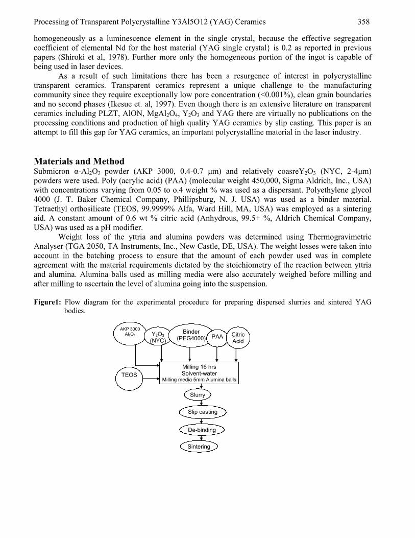
Processing of Transparent Polycrystalline Y3Al5O12 (YAG) Ceramics 358

homogeneously as a luminescence element in the single crystal, because the effective segregation coefficient of elemental Nd for the host material (YAG single crystal is 0.2 as reported in previous papers (Shiroki et al, 1978). Further more only the homogeneous portion of the ingot is capable of being used in laser devices.

As a result of such limitations there has been a resurgence of interest in polycrystalline transparent ceramics. Transparent ceramics represent a unique challenge to the manufacturing community since they require exceptionally low pore concentration (<0.001%), clean grain boundaries and no second phases (Ikesue et. al, 1997). Even though there is an extensive literature on transparent ceramics including PLZT, AlON, MgAl2O4, Y2O3 and YAG there are virtually no publications on the processing conditions and production of high quality YAG ceramics by slip casting. This paper is an attempt to fill this gap for YAG ceramics, an important polycrystalline material in the laser industry. Materials and Method Submicron α-Al2O3 powder (AKP 3000, 0.4-0.7 µm) and relatively coasreY2O3 (NYC, 2-4µm) powders were used. Poly (acrylic acid) (PAA) (molecular weight 450,000, Sigma Aldrich, Inc., USA) with concentrations varying from 0.05 to o.4 weight % was used as a dispersant. Polyethylene glycol 4000 (J. T. Baker Chemical Company, Phillipsburg, N. J. USA) was used as a binder material. Tetraethyl orthosilicate (TEOS, 99.9999% Alfa, Ward Hill, MA, USA) was employed as a sintering aid. A constant amount of 0.6 wt % citric acid (Anhydrous, 99.5+ %, Aldrich Chemical Company, USA) was used as a pH modifier.

Weight loss of the yttria and alumina powders was determined using Thermogravimetric Analyser (TGA 2050, TA Instruments, Inc., New Castle, DE, USA). The weight losses were taken into account in the batching process to ensure that the amount of each powder used was in complete agreement with the material requirements dictated by the stoichiometry of the reaction between yttria and alumina. Alumina balls used as milling media were also accurately weighed before milling and after milling to ascertain the level of alumina going into the suspension. Figure1: Flow diagram for the experimental procedure for preparing dispersed slurries and sintered YAG

bodies.

Milling 16 hrs Solvent-water

Milling media 5mm Alumina balls

AKP 3000 Al2O3

TEOS

Y2O3 (NYC)

Binder (PEG4000) PAA Citric

Acid

Slurry

Slip casting

De-binding

Sintering

359 Kwadwo A. Appiagyei

Table 1: Dispersant (PAA) concentrations (wt. % based on solids content) Sample code Y1 Y2 Y3 Y4 Y5 Y6 PAA wt % 0.1 0.15 0.20 0.25 0.30 0.35

Slurries were prepared as illustrated in the flow diagram in Fig. 1. Detailed information about the dispersant (PAA) concentrations used is as reported in Table 1. After drying the slip cast samples binder burn-out was carried out at 600oC to remove all the organic additives. Sintering was carried out at temperatures in the range of 1750-1800oC for periods ranging between 8-16 hours. The slurries or suspensions were tested to determine their rheological behaviour using rotational stress controlled rheometer ( Carimed CSL 100, New Castle, De, USA). All measurements were done at a constant temperature (25oC) using the cone and plate configuration. Measurements were taken up to a shear rate of 500/s.

X-Ray diffraction analysis was carried out on the sintered sample using XRD(Sintag Inc, USA) at a current in-put of 30mA and a voltage of 35 kv. Microstructural analysis was carried out using scanning electron microscope. Results Figs. 2a and b show the SEM micrographs of the starting powders, AKP 3000 alumina and NYC yttria respectively. The Y2O3 was relatively coarser than the alumina hence the need for long milling to reduce the particle size. The results of TGA analysis for alumina and yttria are as shown in Figs. 3 and 4. Rheological behaviour of colloidal dispersion is among their most important properties. Rheological measurements monitor changes in flow behaviour in response to an applied stress or strain. Results of the shear stress vs. shear rate measurements are as illustrated in Fig. 5.

Figure 2a: SEM Micrograph of APK 3000 Alumina Figure 2b: SEM Micrograph NYC yttria

Processing of Transparent Polycrystalline Y3Al5O12 (YAG) Ceramics 360

Figure 3: TGA of NYC Y2O3

Figure 4: TGA of AKP 3000 Alumina

Fig. 6 shows the X-Ray diffraction of a YAG sintered sample. Fig. 7 is the SEM micrograph of a YAG sample showing the presence of a second phase. Fig. 8 is the energy dispersive analysis (EDAX Analysis) which indicates that the second phase was excess alumina. Figs. 9 and 10 show the SEM of samples made from agglomerated non-Newtonian slurry and that made from a Newtonian-like slurry respectively. The transparency of the sample made from Newtonian-like slurry is shown in Fig.11 and Fig.12 shows the transparency of a sample made from agglomerated non-Newtonian slurry. Discussion Weight changes during the TGA analysis are as shown in Figs. 3 and 4. The difference in the weight losses was taken into consideration during batching to avoid samples that are either alumina or yttria rich. Alumina or yttria rich samples did not give the expected transparency. The reaction between alumina and yttria to form yttrium aluminium garnet (YAG) proceeds according to the chemical equation:

3Y2O3 + 5 Al2O3 → 2Y3Al5O12 (1) From equation 1 the amount of yttria and alumina required for the reaction to proceed

stoichiometrically is: 57.06% and 42.94% respectively. Deviations from this lead to bodies which have either alumina in excess or yttria in excess. A sample typical of alumina excess is as illustrated in Fig. 7. The excess material acts as a second phase and hence as a scattering center (19) which tends to

361 Kwadwo A. Appiagyei

prevent the body from being transparent. Thus, during batching the difference in the weight losses illustrated by Figs. 3 and 4 must be compensated for to enhance a good stoichiometric balance. A weight change of the alumina milling media was determined and this was also compensated for during the batching to avoid any imbalance in the stoichiometric ratio.

Figure 5: The Effect of Dispersant Concentration on the Rheological Behaviour of YAG Suspensions.

0

5

10

15

20

25

0 50 100 150 200 250 300 350 400 450 500Shear rate (1/s)

Shea

r str

ess

(Pa)

Y6

Y5

Y4

Y3

Y2

Y1

Results showing the rheological behaviour of the slurries containing various levels of dispersant is as shown in Fig.5. The apparent viscosity η is related to the applied shear stress τ and the shear rate γ by the following expression:

τ = ηγ (2) Two types of flow behaviour can be observed under steady shear depending on suspension

composition and stability as shown in Fig. 5. Newtonian-like behaviour, the simplest flow response, where viscosity is independent of shear rate is displayed in Fig. 5. With the exception of the slurry which contained 0.1 wt % PAA that exhibited Newtonian flow (Y1) all the rest showed pseudoplastic or shear thinning behaviour. Pseudoplastic or shear thinning behaviour occurs when the viscosity decreases with the shear rate.

Fig. 6 shows the XRD analysis of the sintered samples. All the peaks are YAG peaks indicating that there was a complete transformation of the bodies to the cubic YAG phase.

Figure 6: XRD of YAG sintered sample

0

100

200

300

400

500

600

15 20 25 30 35 40 45 50 55 60 65

2θ/θ

cps

Processing of Transparent Polycrystalline Y3Al5O12 (YAG) Ceramics 362

Figure 7: SEM Micrograph of YAG showing Alumina excess

Figure 8: EDAX Analysis showing the analysis of bright spots in Fig. 7 above

Figure 9: SEM Micrograph of a YAG sample made from agglomerated non-Newtonian slurry

363 Kwadwo A. Appiagyei

Figure. 10: SEM Micrograph of a YAG sample made from a Newtonian-like slurry.

Fig. 8 shows the EDAX analysis of the bright spots (in Fig. 7) which were found to be very rich in alumina. The excess alumina acts as a second phase and therefore a scattering center thus making this sample poor in transparency (Ikesue et al, 1997). Fig. 9 is the SEM micrograph of a sample that was prepared from slurry with pseudo-plastic non-Newtonian characteristics. The density of this sample was very poor (<90%) because of the large pores that evolved as a result of the presence of large agglomerates in the slurry used for casting the sample.

Figure. 11: A picture showing the transparency of a sintered YAG body made from a well dispersed slurry.

Figure 12: A picture showing the transparency of a sample made from a slurry that was not well dispersed.

Processing of Transparent Polycrystalline Y3Al5O12 (YAG) Ceramics 364

Fig.10 is the SEM micrograph of a sample that was prepared from homogeneous Newtonian-like slurry. This sample showed an excellent transparency as illustrated in Fig. 11. Slurries with stoichiometric imbalance and those that were non-Newtonian with agglomerates showed poor transparency as shown in Fig. 12.

From the foregoing it can be concluded that dispersant concentration has a lot of influence on the rheology of the aqueous YAG slurries which in turn influence the transparency of the final product. Well dispersed slurries tend to give transparent samples. Agglomerated slurries, however, tend to give porous samples with very poor transparency. Also samples with incorrect Al2O3/Y2O3 stoichiometric ratios tend to be rich in either alumina or yttria and such samples, irrespective of whether alumina or yttria is in excess, tend to be poor in transparency. Acknowledgement The author, who conducted this research at the Materials Science and Engineering Department at Pennsylvania State University, USA, expresses his sincere gratitude to Prof Gary messing and his research group for providing him with all the needed support and encouragement.

365 Kwadwo A. Appiagyei

References [1] T. H. Maiman, Simulated Optical Radiation in Ruby, Nature (London), 187(August 6) 493-94

(1960) [2] T. H. Maiman, Optical and Microwave- Optical Experiments in Ruby, Phy. Rev. Lett. 4 (11)

564-66 (1960) [3] P. F. Moulton, Spectroscopic and Laser Characteristics of Ti: Al2O3, J. Opt. Soc. Am. B., 3 (1)

125-32 (1986) [4] G. Huber, E. W. Duczynski and K. Petermann, Laser pumping of Ho-, Tm-, Er-doped garnet

lasers at room temperature, IEEE J. Quantum Electron 24(6), 920-23 (1988) [5] T. Y. Fan, G. Huger, R. L. Byer and P. Mitzsch erlich, Spectroscopy and diode laser-pumped

operation of Tm, Ho: YAG, IEEE J. quantum electron, 24 (6) 924-33(1988) [6] J. E. Geusic, H. M. Marcos and L. G. van Uitert, laser oscillation in Nd-doped Yttrium

Aluminum and Gadolinum Garnets, Appl. Phys. Lett., 4 (10) 182-84 (1964). [7] C. Greskovich and K. N. Wood, Fabrication of Transparent ThO2-doped Y2O3, Am. Ceram.

Soc. Bull. 52(5), 473-78 (1973) [8] C. Greskovich and J. P. Chernoch, Polycrystalline Ceramic Laser, J. Appl. Phy., 45 (10) 4599-

606. (1973). [9] C. Greskovich and J. P. Chernoch, Improved Polycrystalline laser, J. Appl. Phys. 45(10) 4495-

502(1974). [10] G. de With and H. J. A. van Dijk, Translucent Y3Al5O12 Ceramics, Mat. Res. Bull. 19(12),

1669-74(1984) [11] C. A. Mudler and G. de With, Translucent Y3Al5O12 Ceramics, Electron microscopy

Characteristics, solid state Ionics, 16, 81-86 (1985). [12] M. Sekita, H. Haneda, T. Yanagitani and S. Shirasaki, Induced Emission Cross Section of

Nd:YAG Ceramics, J. Appl. Phys. 67(1), 453-58(1990). [13] N. Daikuzano, Present and Future of Medical YAG laser, Rev. laser Engineering, 21(8), 894-95

(1993). [14] Hofstetter, K. Rothenbeger, E. Keidtsch et.al., Proceedings of the 4th Congress of the

international Society for laser surgery, vol.10, pp 18-20, Laser Tokyo, Tokyo, Japan, 1981. [15] N. Daikuzono and S. N. Joffe, Artificial sapphire probe for contact photo-coagulation and

tissue vaporization with the Nd: YAG laser Med. Instrum., 19, 173-78(1985). [16] N. Goto and H. Ito, High average power 266nm generation of Nd:YAG laser and its industrial

applications, Rev. laser Eng.,m21(8) 885-93 (1993). [17] K. Ueda and N. Uehara, Frequency stabilization of LD-pumped YAG lasers for

gravitationalwave detection, Rev. Laser Eng., 21 (8), 859-72(1993). [18] K. Shiroki and Y. Kuwano, An effective neodymium segregation coefficient in neodymium-

doped yttrium-aluminium-garnet crystal growth by pulling method, Nippon Kagaku Kaishi, 7, 940-44(1978).

[19] Ikesue, K. Yoshida, T. Yamamoto and I. Yamaga, Optical Scattering center in polycrystalline Nd:YAG laser, J. Am. Ceram. Soc., 80(6) 1517-27(1997).

European Journal of Scientific Research ISSN 1450-216X Vol.15 No.3 (2006), pp. 366-372 © EuroJournals Publishing, Inc. 2006 http://www.eurojournals.com/ejsr.htm

A New Algorithm for Locating Tandem Repeats in a DNA

Sequence

Ziad A. A.Alqadi Faculty of Technological Engineering

Al Balqa Applied University, Amman, Jordan

Musbah Aqel Faculty of Engineering

Applied Science University, Amman, Jordan E-mail: musbahaqel@yahoo.com

Ibrahiem M. M. El-Emary

Faculty of Engineering Al Ahliyya Amman University, Amman, Jordan

E-mail: doctor_ebrahim@yahoo.com

Abstract

An algorithm for locating tandem repeats in DNA sequence is proposed based on string matching techniques to find the repetition of a tandem in a selected DNA sequence. The algorithm was implemented and compared with other algorithms like Boyer-Moore algorithm .Our results show that the proposed algorithm has a better performance in average and worst cases relative to others. Also, the results indicate that the proposed algorithm has less time complexity and decrease in computation time process. Keywords: DNA, BM, TBM, CAT, and TAG

1. Introduction Deoxyribonucleic Acid (DNA) is primary genetic material of all living organisms [1]. Its molecule usually consists of two nucleotide strands connected by base pairs, where the base of DNA is: Adenine (A), Cytosine (C), Guanine (G), and Thymine (T). A DNA sequence is represented by a string of four alphabets: A, C, G, and T as the above based. DNA of all living organisms are collected and kept in a database. A very well known DNA, developed by National center for Biotechnology Information is called Genbank [2], which contains huge information of various biological data. In the field of bioinformatics, similarity search is an important algorithm for analyzing biological data sequences. Basically, it is used to find sequences in a database that parts of it are similar to a query sequence. Design approaches of many matching algorithms, such as: Boyer-Moore (BM) algorithm , modified BM algorithm and Turbo Boyer-Moore algorithm(TBM) are based on dynamic programming [3,4], so, the execution time is proportional to number of comparisons, which depends on the sequence size(n) , and the pattern size (m) [5].

DNA typing, with its extremely high power is used to differentiate one human being from another, that is based on a large body of scientific principles and techniques that are universally

A New Algorithm for Locating Tandem Repeats in a DNA Sequence 367

accepted. These newer molecular techniques permit the study of human variability at the most basic level, that of the genetic material itself, DNA. Standard techniques of population genetics and statistics can be used to interpret the results of forensic DNA typing. Because of the newness of the techniques and their exquisite discriminating power, the courts have subjected DNA evidence to extensive scrutiny.

If the array of DNA markers used for comparison is large enough, the chance that two different persons will share all of them becomes vanishing small. With appropriate DNA test systems, the uniqueness of any individual on the planet (except an identical twin) is likely to be demonstrable in the near future. In the meantime, the justification for an inference that two identical DNA profiles come from the same person rests on probability calculations that employ principles of population genetics. Such calculations are, of course, subject to uncertainty. 2. Basic Genetic Principles Each human body contains an enormous number of cells, all descended by successive divisions from a single fertilized egg. The genetic material, DNA, is in the form of microscopic chromosomes, located in the inner part of the cell, the nucleus. A fertilized egg has 23 pairs of chromosomes; one member of each pair comes from the mother and the other from the father. The two members of a pair are said to be homologous. Before cell division, each chromosome splits into two. Because of the precision of chromosome distribution in the cell-division process, each daughter cell receives identical chromosomes, duplicates of the 46 in the parent cell. Thus, each cell in the body should have the same chromosome makeup [8]. This means that cells from various tissues, such as blood, hair, skin, and semen, have the same DNA content and therefore provide the same forensic information. There are some exceptions to the rule of identical chromosomes in every cell, but they do not affect the conclusion that diverse tissues provide the same information [9].

The most important exception occurs when sperm and eggs are formed. In this process, each reproductive cell receives at random one representative of each pair, or 23 in all. The double number, 46, is restored by fertilization. With the exception of the sex chromosomes, X and Y (the male-determining Y is smaller than the X); the two members of a pair are identical in size and shape. (It might seem puzzling that sperm cells, with only half of the chromosomes, can provide the same information as blood or saliva. The reason is that DNA from many sperm cells is analyzed at once, and collectively all the chromosomes are represented).

A chromosome is a very thin thread of DNA; surrounded by other materials, mainly protein (DNA stands for deoxyribonucleic acid). The DNA in a single chromosome, if stretched out, would be an inch or more in length. Remarkably, all that length is packed into a cell nucleus some 1/1,000 inch in diameter. The DNA is compacted by coils within coils.

The DNA thread is actually double, consisting of two strands twisted to form a helix as shown in Fig.1. Each strand consists of a string of bases held together by a sugar-phosphate backbone. The four bases are abbreviated A, T, G, and C (these stand for Adenine, Thymine, Guanine, and Cytosine, but we shall employ only the abbreviations). In double-stranded DNA, the bases line up in pairs, an A opposite a T and a G opposite a C:

C A T T A G A C T G A T G T A A T C T G A C T A

Thus, if the sequence of bases on one strand is known, the other is determined. Prior to cell division, the double strand splits into two single strands, each containing a single

base at each position. There are free-floating bases in the cell nucleus, and these attach to each single strand according to the A-T, G-C pairing rule. Then they are tied together and zipped up by enzymes.

368 Ziad A. A.Alqadi, Musbah Aqel and Ibrahiem M. M. El-Emary

Figure 1a: Chromosome sketch with a small region expanded to show the double-helical structure of DNA. The steps of the twisted ladder are four kinds of base pairs, AT, TA, GC, or CG.

In this way, each DNA double helix makes a copy of itself. There are then two identical double strands, each half old and half new, and one goes to each daughter cell. That accounts for the uniformity of DNA makeup throughout the body. The total number of base pairs in a set of 23 chromosomes is about 3 billion.

A gene is a stretch of DNA, ranging from a few thousand to tens of thousands of base pairs, that produces a specific product, usually a protein. The order of the four kinds of bases within the gene determines its function. The specific base sequence acts as an encoded message written in three-letter words, each specifying an amino acid (a protein building block). In the diagram above, CAT specifies one amino acid, TAG another, ACT a third, and so on. These amino acids are joined together to make a chain, which folds in various ways to make a three dimensional protein. The gene product may be detected by laboratory methods, as with blood groups, or by some visible manifestation, such as eye color.

The position that a gene occupies along the DNA thread is its locus. In chemical composition, a gene isn’t different from the rest of the DNA in the chromosome. Only it’s having a specific sequence of bases, enabling it to encode a specific protein, makes each gene unique. Genes are interspersed among the rest of the DNA and actually compose only a small fraction of the total. Most of the rest has no known function.

Alternative forms of a gene, for example those producing normal and sickle cell hemoglobin, are called alleles. The word genotype refers to the gene makeup. A person has two genes at each locus, one maternal, one paternal. If there are two alleles, A and a, at a locus, there are three genotypes, AA, Aa, and aa. The word genotype can be extended to any number of loci. In forensic work, the genotype for the group of analyzed loci is called the DNA profile. (We avoid the word fingerprint to prevent confusion with dermal fingerprints). If the same allele is present in both chromosomes of a pair, the person with that pair is homozygous. If the two are different, the person is heterozygous. (The corresponding nouns are homozygote and heterozygote.) Thus, genotypes AA and aa are homozygous and Aa is heterozygous.

Genes on the same chromosome are said to be linked, and they tend to be inherited together. They can become unlinked, however, by the process of crossing over, which involves breakage of two homologous chromosomes at corresponding sites and exchange of partners. Genes that are on no

A New Algorithm for Locating Tandem Repeats in a DNA Sequence 369

homologous chromosomes are inherited independently, as are genes far apart on the same chromosome.

Occasionally, an allele may mutate; that is, it may suddenly change to another allele, with a changed or lost function. When the gene mutates, the new form is copied as faithfully as the original gene, so a mutant gene is as stable as the gene before it is mutated. Most genes mutate very rarely, typically only once in some 100,000 generations, but the rates for different genes differ greatly. Mutations can occur in any part of the body, but our concern is those that occur in the reproductive system and therefore can be transmitted to future generations. 3. Proposed Algorithm for Locating Tandem Repeats In this paper, an algorithm is developed for locating repetitive regions within DNA sequences. Identifying and locating repeats will help biologists learn more about repetitive regions. In addition, computational analysis of DNA sequences becomes increasingly complex when repetitive DNA occurs in the sequences under analysis. Thus, identification of repetitive DNA is a first step towards enabling biologists to understand DNA sequences and computational biologists to solve more complex analysis problems involving DNA sequences [7].

Tandem repeats are one type of repetitive DNA. It is a string of characters which recur consecutively within a larger string. In biological terms, it is a concatenation of basic units within a DNA sequence where the DNA sequence and basic unit are composed of the bases: A, C, G and T.

A tandem repeat can occur at any position in the DNA sequence. It can start with any base in the basic unit but must continue the repeat with the next base in the basic unit. For example, the tandem repeat CAGGCAGGCAGGCAG has a basic unit of GGCA. The region begins with C and continues with A, the next base in the basic unit. (Note: the subsequent base is the first base in the basic unit. This is what is meant by a concatenation of basic units.) Practical issues. 3.1 Description of the Proposed Algorithm

The proposed algorithm requires the following steps to be implemented:- 1. Select the Tandem P with length (m) to be find in a DNA sequence. 2. Select the master DNA sequence F with length (n). 3. Find the locations of P (1) in F. 4. Find the locations of P (m) in F. 5. For each pair of locations P (1) and P (m) calculate the distant between the two locations. 6. Ignore all the distances which are less than m or greater than m. 7. Compare each subsequence of F (with distant = m) with the selected sequence P, if they are equal

then save the position of P(1) as a starting index of the matched sequence. Thus after running this algorithm, we can obtain valuable information which can be used for

finding the similarity and to perform some analysis on DNA sequence.

3.2 Algorithm Implementation

The proposed algorithm uses dynamic programming to locate all tandem repeats which have a basic unit as specified in the input file. The output can be used in conjunction with a graphing program to identify plateaus. These plateaus represent tandem repeat regions. Dynamic Programming is a two -pass process which combines traditional dynamic programming with a second pass to wrap scores within a row. It is the second pass which is critical for identifying tandem repeats.

The following shows some results of detecting tandem in a DNA sequence. We have to notice that there are no modifications in the algorithm in order to perform the way of matching (using the direct match from beginning to end or using the reverse match from end to beginning)

370 Ziad A. A.Alqadi, Musbah Aqel and Ibrahiem M. M. El-Emary

sample sequence one ttaaggaccccatgccctcgaataggcttgagcttgccaattaacgcgcacgggctggccgggcgtataagccaaggtgtagtgaggttgcattatacatgccggcttgtgattaacgcatgccataggacggttaggctcagaacccgcaaccaatacacgtgattttctcgtcccctg

Results for 180 residue sequence "sample sequence one" starting "ttaaggaccc" >match number 1 to "ttaa" ends at position 4 on the direct strand ttaa >match number 2 to "ttaa" ends at position 44 on the direct strand ttaa >match number 3 to "ttaa" ends at position 116 on the direct strand ttaa >match number 4 to "ttaa" ends at position 68 on the reverse strand ttaa >match number 5 to "ttaa" ends at position 140 on the reverse strand ttaa >match number 6 to "ttaa" ends at position 180 on the reverse strand ttaa

sample sequence two aggcgtatgcgatcctgaccatgcaaaactccagcgtaaatacctagccatggcgacacaaggcgcaagacaggagatgacggcgtttagatcggcgaaatattaaagcaaacgacgatgacttcttcgggaaattagttccctactcgtgtactccaattagccataacactgttcgtcaagatatagggggtcacccatgaatgtcctctaaccagaccatttcgttacacgaacgtatct

Results for 243 residue sequence "sample sequence two" starting "aggcgtatgc" >match number 1 to "gat" ends at position 13 on the direct strand gat >match number 2 to "gat" ends at position 78 on the direct strand gat >match number 3 to "gat" ends at position 92 on the direct strand gat >match number 4 to "gat" ends at position 119 on the direct strand gat >match number 5 to "gat" ends at position 185 on the direct strand gat >match number 6 to "gat" ends at position 4 on the reverse strand gat >match number 7 to "gat" ends at position 153 on the reverse strand gat >match number 8 to "gat" ends at position 232 on the reverse strand gat

sample sequence three tactcagggctccagaggtacaagttggtaatcggttaggtgtatcgccgccaggggtgcgtcgtcatgactcggttaga

Results for 80 residue sequence "sample sequence three" starting "tactcagggc" >match number 1 to "tcat" ends at position 68 on the direct strand tcat >match number 2 to "tcat" ends at position 14 on the reverse strand tcat

3.3 Experimental Results

The proposed algorithm was implemented using different DNA sequences in size, and it was compared with TBM algorithm, which was also executed using the same files.

Tables (1-6) show the obtained results, (number of comparisons and CPB (Comparisons per Byte) which is equal the number of comparisons divided by the DNA sequence size).

A New Algorithm for Locating Tandem Repeats in a DNA Sequence 371

Table 1.1: DNA sequence size=103337 P length(m)(Tandem) TBM algorithm TBM CPB Developed algorithm Developed CPB

1 206674 2 99004 0.96 2 162084 1.57 86892 0.84 3 119658 1.16 89232 0.86 4 107856 1.04 89132 0.86

Table 1.2: DNA sequence size=70182 P length(m)(Tandem) TBM algorithm TBM CPB Developed algorithm Developed CPB

1 140364 2 67468 0.96 2 110088 1.57 59034 0.84 3 81276 1.16 60444 0.86 4 73163 1.04 60438 0.86

Table 1.3 DNA sequence size=36578 P length(m)(Tandem) TBM algorithm TBM CPB Developed algorithm Developed CPB

1 73156 2 35248 0.96 2 57373 1.57 30814 0.84 3 42398 1.16 31470 0.86 4 38112 1.04 31588 0.86

Table 1.4: DNA sequence size=19900 P length(m)(Tandem) TBM algorithm TBM CPB Developed algorithm Developed CPB

1 39800 2 19516 0.98 2 31227 1.57 16913 0.85 3 23074 1.16 16996 0.85 4 20696 1.04 17161 0.86

Table 1.5: DNA sequence size=5578 P length(m)(Tandem) TBM algorithm TBM CPB Developed algorithm Developed CPB

1 11156 2 5436 0.97 2 8754 1.57 4791 0.86 3 6444 1.16 4756 0.85 4 5803 1.04 4990 0.89

Table 1.6: DNA sequence size=2480 P length(m)(Tandem) TBM algorithm TBM CPB Developed algorithm Developed CPB

1 4960 2 2436 0.97 2 3870 1.57 2121 0.86 3 2877 1.16 2137 0.85 4 2585 1.04 2219 0.89

372 Ziad A. A.Alqadi, Musbah Aqel and Ibrahiem M. M. El-Emary

4. Conclusions A matching algorithm was proposed based on string matching for locating tandem repeats of DNA sequence. It was implemented and compared with other algorithms like TBM. Our algorithm has shown better performance, and valuable outputs which can be used later for analysis purposes.

The time complicity of the algorithm (worst case) is always less than O(n), and the proposed algorithm decreases the computation times from 1.7 to 2.06 times comparing with TBM algorithm.

Also we can see from the obtained results that the time complexity does not depend on the DNA sequence size, but it depends on the tandem size. References [1] Sirinawin, J. 1995. The Structure and Function of Gene and Chromosome. Essential

Medical Genetics. 3. [2] National Center for Biotechnology Information (NCBI). 2000. Basic Local Alignment Search

Tool (BLAST), http://www.ncbi.nim.nih.gov [3] Crochemore, M., 1997. Off-line Serial Exact String Searching in Pattern Matching Algorithms,

ed. A. Apostolico and Z. Galil, Chapter 1, pp 1-53, Oxford University Press [4] Crochemore, M ., Czumaj, A., Gasieniec, L., Jarominek, S., Lecroq, T., Plandrowski, W., Rytter,

W., 1994, Speeding up Two String Matching Algorithms, Algorithmica 12(4/5):247-267 [5] Sirinawin, J. 1995. The Structure and Function of Gene and Chromosome. Essential

Medical Genetics. 3. [6] Allen R, Balding D, Donnelly P, Friedman R, Kaye D, LaRue L, Park R, Robertson B, Stein A.

1995. Probability and Proof in State v Skipper: an Internet Exchange. Jurimetrics J 35: 277-310.

[7] Fischetti, V.A., etal. ``Identifying Periodic Occurrences of a Template with Applications to Protein Structure.'' . Proceeding of the Third Annual Symposium on Combinatorial Pattern Matching. AprMay 1992. Arizona. pp111120 (Wendt Library) or pp109118 (Debby).

[8] Giegerich, R. and Wheeler D., “Pairwise sequence alighnment”, Biocomputing Hypertext Course Book. www.techfak.uni-bielefeld.de/bcd/Curric/PrwAli/prwali.html, May 21, 1996.

[9] Yang, R. “Multiple Protein /DNA Sequence Alignment with Constraint Programming”. Proceeding of the fourth international conference on the practical application of constraint technology, 4:159-166, 1998.

European Journal of Scientific Research ISSN 1450-216X Vol.15 No.3 (2006), pp. 373-380 © EuroJournals Publishing, Inc. 2006 http://www.eurojournals.com/ejsr.htm

Vibration Analysis using Conversion of Transfer Matrices

Kadhim Hamza Ghlaim Dijlah Colleege University, Mech. Eng. Deptartment

Abstract

A matrix conversion method is proposed to calculate the new eigendata for parameter estimation procedure. The advantages of the method are the applicability to large complex structures, in particular, the concept of breaking up a complicated system into subsystems with simple elastic and dynamic properties, also it is useful one in rendering managible system whose solutions appear obscured in complexity. Since many engineering components are continuous in the way the mass and elasticity is distributed, it is useful to consider such method which involve solving such continuous systems. The objective of the study is to propose a method by which a fore mentioned difficulties can be alleviated. The method will be demonstrated on a realistically complex structural system.

Introduction A common type of system occuring in engineering practic consists of a number of elements linked together end to end in the form of chain, well known examples are continuous beams, turbines, generator shafts, crank shafts, casings,etc. The transfer matrix method (1) is ideally suited to such system. Although the transfer matrix method is suitable for the treatment of branched and coupled system, its application is in advisable for system that lack a predominant chain topology (2). The transfer matrix method analysis has been greatly used by practicing engineers as fully documented in ref (3) to (10). The method becomes too cumbersome when there are too many mass stations or rotors have many bearings, Various schemes have been proposed to overcome the problems because multiplication of matrices makes the algebra grow quickly, so any loss of accuracy in subsequent matrix multiplication may becomes large for complete system. The effect of the loss of accuracy can be eliminated by certain methods (7). Another possibilities is to compute for the shaft separately and join it with bearings through impedance matchings (1,8) in which the shaft is divided into a number of equal lengths, and the mass of each length is concentrated at its centre. In addition, the matrix multiplication of the complete system includes the transfer matrix of the connection points.

Numerical difficulties can arise in using the transfer matrix method when high frequencies are encountered or a large number of elements exist. The difficulty, in common with those found in other methods of analysis, occurs due to the solution depending upon the small difference in large numbers. These large numbers increase with each subsequent matrix multiplication. The transfer matrix method can be modified to overcome this contingency by assuming an initial state vector (9). This vector need not be close to the actual vector since, with one iteration, the vector is extremely near the actual value and if desired this corrected value can be used throughout a second iteration.

Unfortunately none of these methods are convenient for the problem which is to be tackled. This requires all the eigenvalues and eigenvectors of a particular component. The methods outlined above all give approximate values of eigenvalues and eigenvectors. For this reasons a version of transfer matrix technique which could be used in the matrices eigenproblem (10), [A] W=λ [B]W was searched for. Fortunately such a version has been described in this paper where it demonstrates

Vibration Analysis using Conversion of Transfer Matrices 374

how the transfer matrix method can be converted to mass-stiffness matrices and it is quite essential in this work were a specific problem is solved an this technique proved to be so efficient. Development of Transfer Matrix to Produce Mass and Stiffness Matrices

To demonstrate this method let us consider the system shown in Fig 1., in which the bodies on beams are consider to have both mass and rotary inertia and it is assumed to be vibrating with frequency ω .

Consider the equations of Ref (1) page 55 to 58, for node 1 in Fig 1 and Fig (3-A). gives :- R

W1 = 11111 θθθ === LRL andWW

Since 01 =LV The equation of inertia force is

RVWM 112

1 −=ω (1) And Since 01 =LM

The equation of inertia couple is RMI 11

21 −=θω (2)

Applying the equations of state vector to the mass less beam between node 1 and node 2 Fig 1 and Fig 3-B.

RRRRL VEJlM

EJllWW 1

3

1

2

112 62+++−=− θ (3)

RRRL VEJlM

EJl

1

2

112 2++= θθ

(4) RRL lVMM 112 += (5)

RL VV 12 = (6)

Equations (3) and (4) can be manipulated to give :

LRLR

lEJw

lEJW

lEJV 2213231

61212 θ+−= (7)

LRRLR

lEJ

lEJW

lEJW

lEJM 2112221

2466 θθ −−+= (8)

Then equation (5) becomes

LRRLL

lEJ

lEJW

lEJW

lEJM 211222

24266 θθ ++−= (9)

And equation (1) and (2) becomes

LRLR

lEJ

lEJW

lEJW

lEJWM 221223131

21

661212 θθω −−−= (10)

LRRL

lEJ

lEJW

lEJW

lEJI 2112221

21

2466 θθθω ++−= (11)

In a Similar fashion the application of the equations to node 2 and the mass less beam between node 1 and node 3 produces

375 Kadhim Hamza Ghlaim

RL VVWM 2222

2 −=ω (12)

RL MMI 2222

2 −=θω (13) RL WW 22 = (14)

RL22 θθ = (15)

RRRRL VEJlM

EJlWW 2

3

2

2

223 62+++−=− θ (16)

RRRL VEJlM

EJl

2

2

223 2++= θθ (17)

RRL lVMM 223 += (18)

RL VV 23 = (19)

From these equations obtain the following RLRLR

lEJ

lEJW

lEJW

lEJV 223323332

661212 θθ ++−= (20)

LRRLR

lEJ

lEJW

lEJW

lEJM 3222322

2466 θθ +−+= (21)

and

LRRLL

lEJ

lEJW

lEJW

lEJM 3222323

4266 θθ ++−= (22)

Substituting the relevant terms into equations (12) and (13) gives

RLRRL

lEJ

lEJW

lEJW

lEJW

lEJWM 12321323332

22

66122412 θθω +−−+= (23)

and

RLRRL

lEJ

lEJ

lEJW

lEJW

lEJI 13212322

22

22866 θθθθω +++−= (24)

Aplying equations above to node 3 is Similar to the way applied to node 1 because 03 =RM and

03 =RV , then equations reduces to

RLRL

lEJ

lEJW

lEJW

lEJWM 323223333

23

661212 θθω ++−= (25)

LRRL

lEJ

lEJW

lEJW

lEJI 3222323

23

4466 θθθω ++−= (26)

In situation where the moments of inertia are not zero, then equations 10,11,13,24,25, and 26 are written directly in matrix form [A] W = λ [B] W as follows;

Vibration Analysis using Conversion of Transfer Matrices 376

(27)

Where λ = 2ω

Worked Problem In the actual case in fig.2 moments of inertia are zero, M1=M=100 kg, M2 = 2M = 200 kg, M3 = M = 100 kg, EJ = 109 N.m2, L = 1 m

Equations 10,24 and 26 can be manipulated to give

3211 41

23

45 W

lW

lW

l+−=θ (28)

312 21

21 W

lW

l−=θ (29)

1323 41

45

23 W

lW

lW

l−−=θ (30)

Substituting these equations into 10,23 and 25 obtaining the Simultaneous equations

3231312

233

23 W

lEJW

lEJW

lEJWM +−=ω (31)

33231322 3632 W

lEJW

lEJW

lEJWM −+−=ω (32)

33231332

233

23 W

lEJW

lEJW

lEJWM +−=ω (33)

Setting up these equations in matrix form as (A) (W) = λ (B) (W),as where

377 Kadhim Hamza Ghlaim

(34)

For the exit eigenvalues and corresponding eigenvectors, compare the eq.34 and eq.27, where the Solution of this matrix equation will give following eigenvalues and corresponding eigenvectors as follow:

The result obtained for eigenvalue is compared with that used by W. Thomson (11) when applying the principle of conservation of momentum, by applying the equation

⎟⎠⎞

⎜⎝⎛ +=

216

3

nMlEJω ; Where

mMn =

96.7745=∴ω rad / sec

Also same result is obtained by using the transfer matrix method ref (1) Conclusions The method of transfer matrices is thus shown capable of producing the relevant mass and stiffness matrices of a system which is vibrating in two or three dimensional. And by converting the transfer matrics to mass and stiffness matrices, as demonstrated, one able to calculate relatively easily the natural frequencies and mode shapes of the system.

This also provides for better storage and Simpler compilation in general and this technique is used for more complicated systems.

Figure 1: Free Ends Beam with concentrated masses and moment of inertia

Vibration Analysis using Conversion of Transfer Matrices 378

Figure 2: Free Ends Beam with concentrated masses

379 Kadhim Hamza Ghlaim

Figure (3-A): Finite element representation of pipe conveying fluid

Figure (3-B): End forces and deflections for massless beam (Free-body sketch span)

Nomenclature: [ M ] Mass matrix [ K ] Stiffness matrix q Displacement Vector ω Component natural frequency I Moment of inertia EJ Bending stiffness Ө and β Angular displacement R Right hand side L Left hand side K Spring stiffness l Length W Linear displacement

Vibration Analysis using Conversion of Transfer Matrices 380

References [1] E.C. Pestel and F.A leckie, " Matrix methods in elastomechanics" mcgraw-Hill, London,

1963,pp.51-95. [2] R.D. Blevins, "Formulas for natural frequency and mode shape ", van nostrand Reinold

Company, 1979 pp-101-200. [3] S. Rubin, " Transmission matrices for vibration and their relation the admittance and

impedance" journal of engineering for industry, Feb-1964, p.9. [4] R. Uhring, "The Transfer matrix method as method structural Analysis Among others" J. Sound

vib. 1966 4(2) 136-184. [5] R. plunkett, "Mechanical impedance methods" proc. A. S. M. E. colloquium dec. 1958 [6] J. W. lund, "Calculation of stiffness and Damping properties of Gas bearing" J. lubri caution

technology [7] M. blada, "Dynamic properties of turboset Rotors " IVTAM symposium, Lynghy, Denmark,

Dynamics of Rotors, Springer-uerlag, Berlin, 1975, pp 27-55. [8] P. G. Morton, "Analysis of Rotors Supported upon many Bearings ", J. mech-Engineering

Science, 1972, 14 (1), 25-33. [9] R. I. Uclean, "Vibration Analysis Using Transfer Matrices" Conference on vibration in Rotating

systems -14-15 the February 1972, university of Bristol pp.32-42. [10] C. B, Moler and G.W STEWART, An algorithm for generalized matrix eigenprobloms. SIAM

J. numer. Anal, Vol. 10, pp.241-256, 1973. [11] W. T. Thomson. Theory of Vibration with application. 2nd edition, George allen and unwin,

1981. Lo

European Journal of Scientific Research ISSN 1450-216X Vol.15 No.3 (2006), pp. 381-385 © EuroJournals Publishing, Inc. 2006 http://www.eurojournals.com/ejsr.htm

Stigmatization of Leprosy and Epilepsy and the Implication for

Sufferers

Muoboghare, P. A Delta State University, Abraka, Nigeria

Ogege, S. O

Delta State University, Abraka, Nigeria

Abstract Supportive interaction is what the affected persons seek from spouse, relatives,

friends and other members of society. Contrarily, leprosy and epilepsy are socially defined as disreputable whose sufferers possess discreditable attributes. On the basis of this social construction of illness, the experience of sufferers becomes increasingly traumatic, not due to pain, impairment and disfigurement only, but the social devaluation and rejection which find expression in an unbridgeable social gap between sufferers and previously intimate persons, role restrictions, loss of self respect, feelings of helplessness and despondency. The paper addresses the whole issue of stigmatization and its implication on symptom management and social functioning and proffers micro and macro options for coping with and ameliorating stigma and its ravaging effects.

Introduction A large and growing body of literature presents detailed discussions of aetiology, symptomatology, treatment and regimens. This outpouring of information however generally ignores a basic aspect of illness especially those defined as chronic. The ignored aspect borders on how to deal with such ailments like leprosy and epilepsy in social terms.

Leprosy and epilepsy are major health problems that are mostly experienced in developing countries. Leprosy is a chronic disease caused by Mycobacterium leprae, an acid and alcohol fast bacillus. Its most common first symptom is a small but persistent area of impaired sensation or numbness. The bacterium affects the peripheral nerves, the skin and in rare cases, the mucous membrane of the respiratory tract. Infected persons have their nerves damaged causing obvious deformity and disability.

Modern medical conceptualisation of epilepsy sees it as a seizure produced by intermittent electron and chemical impulses to the brain (Govan et al, 1981). The causes of epilepsy are mainly idiopathic as medical investigation of patients with epilepsy reveals no cause in many cases (Cull and Will, 1995). Its classical signs are generalised convulsion and a loss of consciousness (Laidlaw et al, 1993), and according to Temkin (1971) and Pelman (1977), these convulsions, even though appear threatening, are not usually lethal. Common factors that precipitate seizures are sleep deprivation, emotional stress, physical and mental exhaustion, loud noise, flickering light, etc. Timble identifies a life threatening variant of epilepsy known as status epilepticus. It exists when seizure occurs without the patient regaining consciousness between attacks.

Stigmatization of Leprosy and Epilepsy and the Implication for Sufferers 382

Though leprosy and epilepsy manifest symptom variation, they have certain elements in common. Both of them are diseases of ancient origin with causal linkage with disreputability, demonic possession, pernicious acts and necromantic attacks. Patients with both diseases are vulnerable to discreditable responses from family and other members of society, the reason for their classification as disreputable diseases.

What constitutes an issue of sociological attention is not the disfigurement, pains, loss of body mobility and the death trajectory associated with the diseases, but rather, from the alteration of the sufferers’ social relationships and the implication of the alteration on symptom management and identity crisis. Sick Role and Social Reproach Illness generally has a potentially disruptive consequence on group or society. Parsons (1951) argues that in order to prevent this disruptive effect, there exists a set of shared cultural norms known as sick role. The essence of the sick role is to legitimize the deviation caused by the illness. Parsons identifies four components of the sick role in the society and these are,

i. i.The sick person is exempted from normal social responsibilities, at least to the extent it is necessary to get well.

ii. ii.The individual is not held responsible for his or her condition and cannot be expected to recover as an act of will.

iii. The person must recognize that being ill is undesirable and must want to recover. iv. The sick person is obligated to seek and cooperate with expert advice, generally that of a

physician. Sick people are not blamed for their illness but must work towards recovery (Parsons, 1960). Illness experience reveals the inapplicability of the sick role to patients of leprosy and epilepsy

in the Nigerian society. Instead of adhering to blame-free component of the sick role, certain negative impressions and evaluations are used on the lepers and epileptics. Consequently, people proceed to relate with them on the basis of expectations derived from these impressions and evaluations. This interaction mode signifies social reproach, a deviation from the normative principles of the sick role. Goffman (1963), sees this response as the root of stigmatization.

Stigmatization is a fundamental variant of symbolic interactionism. It is an act of negatively evaluating with attributes that differ from other members of society. The attributes (leprosy and epilepsy) per se are not the stigma; rather, it is the definition of the situation or the social perception of the attributes. Becker (1963), sees stigma as the way the significant others perceive and define the attributes. Thus upon diagnosis, the non sufferer perceives the afflicted persons as having scores to settle with preternatural (witches and wizards) and supernatural (ancestral, deity and God) forces, a perception that is deeply rooted in the belief system.

This perception and definition of the attributes significantly impair social relationship and interactions. It is in the light of this that Goffman refers to stigma as a language of relationship. Stigma interferes with what otherwise might have been a normal social relationship because of their undesired differences from what has been attributes.

The diagnosis and apparent manifestation of symptoms induce stigmatization from family and other members of society. At the initial stage of illness, family members and close friends try as much as possible to conceal it from public glare. As soon as the illness gets out of hands and symptoms become conspicuous, interaction becomes characterised by discreditable comments and avoidance. Stigmatization and Coping with Crisis Certain chronic diseases are fraught with a constant threat of grave medical crisis. Diabetics for instance can fall into insulin coma and die. Epileptics may go into convulsion and be killed in fire, pool of water, or traffic accident. The death arising from the crisis of epilepsy lies not in the convulsion but

383 Muoboghare, P. A and Ogege, S. O

in the scene of the convulsion. These crises need to be controlled so as to minimize their impacts on the patients. The onus lies with members of the family and friends to be organised around the sufferer. They must be prepared to read and understand the warning signals or signs that portend the crisis. It is fundamentally the first step in helping the sufferer to cope with the crisis.

Relevant to the issue of crisis is how far they can go before dying, how fast the crises appear, the clarity of the advance warning signals, the probability of recurrence, the complexity of the saving operations and the completeness of recovery from them. Granted that these critical issues are favourably disposed of, the sufferer still has a traumatic moment coping with the crisis.

Instead of getting the needed assistance from family members and friends, the epileptic is abandoned to manage or cope with the crisis alone. During convulsions, non sufferers stay far away from the victim or even ignore him or her. Apart from this unnecessary abandonment, people are also warned, out of ignorance, against touching the victim until he regains consciousness. This behaviour is derived from the cultural heritage which forbids touching the epileptic during crises or the leper for fear of contacting the disease.

Ordinarily, epileptics need not suffer physical deformities but for the crisis environment which makes the patient prone to fatal consequences resulting from convulsions. Epileptics are seen with wounds resulting from burns, cuts from sharp objects and water and traffic accidents due to lack of attention during convulsions. The negative social aspect of it is the embarrassment that may emanate from the crisis. Most epileptics regain consciousness only to discover their nudity in a crowd, the reason for epileptics opting for the back stage in life. In some cases, due to their inability to put up with life in the back stage or solitary life, epileptics contemplate suicide which they feel is a panacea to the mortifying moments in their lives. The Burden of Symptom Management The control of symptom, otherwise known as symptom management, extends beyond the frontiers of medical management and adherence to regimens. Most times, due to lack of proximity to medical facilities, the patient and his family members and friends rely upon their own ingenuity in the management of symptoms.

Central to the issue of symptom management is that the patient will be concerned primarily with whether the illness has any impairment on his functioning capacities or is evidencing disfigurement. Major symptoms may affect habits and subsequently call for the redesigning or reshaping of important aspects of the sufferer’s life style. Reshaping activities could be made possible through the efforts of persons around him. A severely deformed and disabled leprosy patient may decide to carefully arrange every object he needs within arms reach. In the same vein, the epileptic, through the assistance of members of his family, has errands run for him, spends very little time in the kitchen to avoid fire accidents and is often in bed to cushion the effects of a fall.

The interference of the sufferers’ lives with social relationships depends largely on a number of factors. The withdrawal of relatives and friends from sufferers may be due to the excessive demands by the patient in relation to symptom management and reshaping of activities. Also, whether the illness is terminal, publicly visible, unpredictable, degree of pain and the nature of regimen for the management of symptoms, are put into consideration. More importantly, the status or the social worth of the person before and during the illness determines how long relatives, spouse and friends get on with him. The moment the sufferer is not favourably disposed to these critical factors or conditions, the basic target of the patient is defeated. The fundamental aim of leprosy or epilepsy patient is not just to stay alive or to keep the symptoms of the disease under control, but to live as normally as possible in the face of the symptoms.

Stigmatization of Leprosy and Epilepsy and the Implication for Sufferers 384

The Border Limits of Stigmatization and the Sufferers’ Response The collective definitional process in which the leprosy and epilepsy patients are described as possessing discreditable attributes does not leave the sufferer in a passive shape. Rather, the stigmatized actively learn the meaning of their attributes or performance through direct exposure to rejection and disapproval from non-sufferers in society.

The perception of stigma or what the putatively stigmatized think of others in relation to reaction inform their series of response to the reproach. The first response to the collective definition is the evaluation of the self or personal identity. The self concept is the totality of our beliefs and feelings about ourselves. Geca (1982) simply sees the self concept as our perception about who we are and this can only be established in our social encounter with others.

The social construction of self identity is derived from what Cooly (1998) refers to as the looking glass self – the way in which a person’s sense of self is derived from the perception of others. The looking glass self of the sufferers is not who they actually are but rather their perception of how non sufferers see them. It is a three step process.

i. The sufferers’ imagination of how their personalities and appearances will be judged by non sufferers or other members of society.

ii. The perception of how the sufferers think they are being judged. They are judged as possessing discreditable attributes.

iii. Based on the perceived judgement, the sufferers experience what Kendall (2001) refers to as social devaluation – the possession of less social value than others in a group or society. Social devaluation becomes acute as sufferers begin to exit roles that are central to their social identity. As a result of this unfavourable evaluation, the self concept begins to diminish. In the face of social devaluation and diminishing self identity, the sufferers are left with no

option but to eventually recreate their social lives on a daily basis in relation to the situation on ground. Central to the recreation of social life is tactical withdrawal from other members of society or social environment as a strategic measure of impression management. In the process of this situational withdrawal, according to Goffman (1968), an unbridgeable social gap between the sufferers and non sufferers is established.

In furtherance of the situational withdrawal, sufferers go in search of persons with similar health problems. The rational behind this action is for the sufferer to have the desired understanding and support that is lacking in the larger society. However, this experience is prevalent among leprosy patients who can afford to form leper colonies due to their numerical strength. It is in this colony that they adopt the beggarly life style as a survival strategy. Being alluded to severe loss of social contact, and by extension, great social isolation, sufferers of disreputable illness opt for speedy death. This is very common because they see an endless time ahead depending on people who are not readily available, increasing social isolation and a purposeless life. In other words, sufferers prefer suicide to staying alive in acute hopelessness. Conclusion The desire for lepers and epileptics to be normal and live conventional lives is hardly or never achieved even when the leprosy patient is already cured. This is due to the cultural context in which they find themselves. This social experience is as traumatic as the agony of pain, deformities and disabilities associated with leprosy and epilepsy.

Granted that leprosy and epilepsy are analytically similar to deviance because both represent threat to effective role performance, reaction from ‘normals’ ought to be different towards illness due to intentionality or wilfulness that is attributable to deviance and not illness. There is no doubt that the social functioning of the leprosy and epilepsy patient is severely jeopardized. The basic components of social functioning – satisfaction with roles in life, feeling of self worth and positive relationships with others, have been impaired due to stigmatization for faults that are unintentional. Considering the extent of stigma and its attendant impact on the sufferers or patients of leprosy and epilepsy, there are

385 Muoboghare, P. A and Ogege, S. O

two options at their disposal. The first option is to enable the sufferers manage the stigma and the second option is aimed at amelioration or eradication of stigma in society.

The stigmatized sufferers should devise a strategy to meet the problem of the social devaluation they suffer from other members of society. This option consists of two strategies. The first strategy is that sufferers should try as much as possible to avoid the ‘normals’ in society. In other words, they should identify with those who possess discreditable attributes who will not use derogatory comments on them. On the other hand, they can interact with normals who are sympathetic in approach.

The second strategy in the sufferers’ solution to stigma is concealment of their identities. Beside the physical concealment of cloaking the symptoms, the sufferers should as well adjust to the role prescription of the non sufferers. The latter can be achieved through artful striving to play extra roles to demonstrate their normality. It should be noted however, that concealment is limited inter-alia by the extent and the frequency of the symptoms.

The second option is a macro level approach. It involves a major overhaul in the value structure of our society by creating re-socialisation avenues that will inculcate on the normals the need to empathise. People should understand that leprosy and epilepsy are like any other form of ill health that is independent of the sufferer’s intention. Singling the lepers and epileptics out for blame and reproach is not a positive measure; rather, it is a conscience-soothing strategy of doing nothing about the problem of lepers and epileptics. References [1] Becker, H.S. (1963) Outsiders. New York: Free Press [2] Cooley, C.H. (1998) “The Social Self – the Meaning of ‘I’” in Hans Joachin S. (Ed), On Self

and Social Organization. Chicago: Chicago University Press. [3] Cull, R.E. and Will, R.G. (1998) “Diseases of the Nervous System” in Edward, C.R.W. et al

(Eds) Principles and Practice of Medicine. Edinburgh: Churchill Livingstone. [4] Gecas, V. (1982) “The Self Concept” in Ralph, H.T. and James, F.S. (Eds) Annual Review of

Sociology. Palo Alto CA: Annual Reviews. [5] Goffman, E. (1963) Stigma: Notes on the Management of Special Identity. New Jersey: Prentice

Hill. [6] Govan, A.T., Macfarlance, P. and Collander, R. (1985) Pathology Illustrated. London:

Longman. [7] Kendall, E.E. (2001) Sociology in Our Times. Belment CA: Wadsworth Publishing Company. [8] Laidlaw, J., Richen, A. and Chadwick, D. (1993) Textbook of Epilepsy. Edinburgh: Churchill

Livingstone. [9] Parsons, T. (1951) The Social System Glencoe: Free Press. [10] Parsons, T. (1960) “Towards a Healthy Maturity” Journal of Health and Social Behaviours,

Vol. 1. [11] Perlman, L.G. (1977) The Person with Epilepsy: Lifestyle, Needs, Expectation. Chicago:

National Epilepsy League. [12] Temkin, O. (1971) The Falling Sickness. Maryland: John Hopkins Press. [13] Trimble, M.R. (1989) Chronic Epilepsy, its Prognosis and Management. Chrehester: John

Willy and Sons.

European Journal of Scientific Research ISSN 1450-216X Vol.15 No.3 (2006), pp. 386-395 © EuroJournals Publishing, Inc. 2006 http://www.eurojournals.com/ejsr.htm

Low-Power MP3 Decoder Implemented in a Xilinx Virtex-4

FPGA

Mehdi Samin Microelectronic and Microsensor Research Laboratory

Faculty of Electrical and computer Engineering Tabriz University, Tabriz, Iran

E-mail: samin_meh@yahoo.com Tel:+98 411 3845751; Fax: +98 411 3842785

Javad Frounchi

Microelectronic and Microsensor Research Laboratory Faculty of Electrical and computer Engineering

Tabriz University, Tabriz, Iran

Abstract

A multi-processor architecture for MP3 decoder is presented which occupies 56% of a Virtex-4 LX15 FPGA from Xilinx. In order to reduce the power consumption of the decoder, the architecture of each block is customized to perform own special function using different parallel processing techniques. The estimated average power consumption of the MP3 decoder is only 11.17 mW for one mono sound channel and the decoding time of a complete frame is 20.8 ms at a chip clock frequency of 5 MHZ. The power consumption is much lower than the commercial single-chip MP3 decoder. Keywords: MP3 decoder, FPGA, power consumption, multi-processors architecture

1. Introduction The MPEG-1 layer-III (MP3) is a highly compressed digital audio format which can compress down a piece of music to approximately 90% of the original size with virtually indistinguishable quality. During the first years of mp3 usage, software decoders were used to decode the mp3 files, but during the last couple of years hardware decoders were employed to decode the mp3 files saved on a Flash memory and to play them. Power consumption is an essential issue in such systems and they are efforts [1-4] to design dedicated decoders in hardware with low power dissipation and less clock cycles.

In this paper, we purpose a multi-processor architecture for MP3 decoder in which each block is customized to perform own special function and the whole hardware including the block RAMs has been implemented in a Xilinx Virtex-4 FPGA to reduce the power consumption of the decoder. 2. MP3 Decoding Process In the MP3 decoding process during several stages an input bitstream is converted into PCM audio samples which can be sent to an external digital-to-analog converter (DAC) to be played. Each MP3 bitstream is divided into small packages, or frames, where each frame contains 26 ms of music data. A

Low-Power MP3 Decoder Implemented in a Xilinx Virtex-4 FPGA 387

frame contains compressed audio data as well as information about how it should be properly decoded. In the ISO/IEC 11172-3 (MPEG-1 audio) standard [5] audio information sampled from one (mono) or two (stereo) sound channels at 32 kHz, 44.1 kHz or 48 kHz frequencies can be encoded.

In this work, only sampling frequency of 44.1 kHz from one mono sound channel is supported. Extension to other sampling frequencies or multi channel sampling can be easily accommodated in this hardware. In the designed chip, an input bitstream is processed by eight blocks which are implemented independent of each other and the output PCM audio samples are formed at the sampling frequency of 44.1 kHz with the IS2 standard which is compatible with the most Digital to Analogue Converters (DACs). The block diagram of the MP3 decoder is shown in Figure 1. The function of each block and their implementation in hardware are described in the following sections.

Figure 1: The block diagram of the MP3 decoder

2.1. Synchronizer

This block accepts the input MP3 bitstream which consists of frames of 26 ms audio information. Each frame contains compressed audio data and some other information such as header, CRC, and side information with specific format. This information contains basic specifications of the main data, bitstream control, and the nformation which is necessary to decode the compressed data. Therefore, this block receives the input bitstream, partitions the different parts, and finally stores each part at the specific location of the chip main memory. 2.2. Huffman decoder

This block decodes the encoding main data according to Huffman decoding scheme [5]. In this technique for the data with more repetition number fewer bits are allocated. Moreover, the scalefactors used to quantize the audio information are extracted. These factors are used in the next block, requantizer, to rescale the original frequency lines (symbols) into 576 original non-scaled frequency lines. The outputs of this block are divided into three parts: Big-values, Count, and Zeros.

Since audio signals has higher amplitude in low frequencies thus in Big-values section, the levels of frequency lines are normally between -15 and +15. For the values higher than this range, encoded bits, called linbits, are included in input bitstream. In Count section which represents higher frequency lines, the levels of the frequency lines are 1, 0, and -1. The highest frequency lines are present in Zero section with zero level. Figure 2 illustrates the output of Huffman decoder block for

388 Mehdi Samin and Javad Frounchi

one frame. To decode information, 4 tables with constants and 32 additional Huffman tables are used in this block.

Figure 2: The output of Huffman decoder block

To design Huffman decoding block, 32 tables are implemented as Block Select RAM are used. Based on the side information of each frame, one of these tables is used and the whole block is controlled by a control unit. To store constant tables which are quite small, LUTs (Look Up Tables) configured as ROM are used on the chip. Since tables 16 to 23 and 24 to 31are the same, one table for each set of tables is stored. Moreover, with omitting one of the tables which inverts the input only, the number of stored tables is reduced from 32 to 17.

The output information in the form of 576 values of 32 bits is stored in the main memory and the scalefactores are put in a special small memory to be used by the requantiser block. 2.3. Requantiser

Requantiser is one of the MP3 building blocks and we are proposing a VLSI efficient implementation of this block to reduce power consumption. Its main function is to rescale the output samples of the Huffman decode block in order to reconstruct 576 original frequency lines. Two separate equations used to rescale the short and long blocks are as followings:

BA

iii isissignxr −⋅⋅⋅= 22)( 434

(1) for short block:

),(__)(8210

winsfsscalfactormutiplierrscalefactoBwindowinsubblockgagainglobalA

b⋅=⋅−−=

for long block:

)()(__210

sfbpretabpreflagsflscalfactormutiplierrscalefactoBgainglobalA

b ⋅+⋅=−=

where isi is the value of the input to the requantiser block read from the main memory and xri is the rescaled value stored in the memory after calculation. The other parameters are obtained from the side information of each frame.

The datapath of the requantiser is controlled by a Moore-type Finite state machine (FSM) which is optimized in both timing and hardware resources. This has accomplished in this way that in each state, some parts of the quations are calculated and then buffered to the next state therefore each signal will be stable for a long period of time and consequently the power consumption will be reduced. Using this technique, execution time of this block increases slightly.

Low-Power MP3 Decoder Implemented in a Xilinx Virtex-4 FPGA 389

To reduce the calculation time of 34iis , a search table calculated using the MATLAB has been

formed. In order to reduce the table size to 1024 and consequently the size of the ROM implemented as a Block select RAM on the chip by a factor of 8, the following relation is used:

3434

816 i

iisis ⋅= (2)

In this way if the isi value is less than 1024, xri is directly obtained from the search table. Otherwise, isi is divided by 8 and then xri obtained from the table is multiplied by 16. 2.4. Reordering

In the stage MDCT of a decoding process, two types of windowing are used. When long windowing is used, 576 frequency lines are ordered in normal form in increasing order of sub-band frequency. When short windowing is used, three different windows are employed therefore in decoding process the frequency lines must be reordered in normal form in this block. The reordering procedure for short blocks is shown in Figure 3.

Figure 3: Reordering procedure for short blocks

To implement this block, two internal memories are employed. One of these memories is used to store the data from the main memory and the other one includes the corrected addresses to restore the data in the main memory. Using this architecture, very short execution time can be achieved. 2.5. Alias-reduction

To compensate for the alias reduction occurs in encoding process due to non-ideal function of the bandpass filters, in this block adjacent frequency lines are mixed together in 8 butterfly filters and thus the values of all frequency lines except two middle lines are altered. Figure 4 illustrates clearly the alias reduction procedure.

390 Mehdi Samin and Javad Frounchi

Figure 4: Alias reduction procedure

To implement this block, a FSM, a butterfly, and several counters have been employed. One of the limitations of this block is multiplier unit for which a multiplier shared by the other blocks has been used on the chip. There is a trade-off between the execution time and the hardware resources and the parallel structures and buffering of the temporary values are employed. The butterfly coefficients are stored in LUTs configured as ROMs. In order to reduce the execution time of multiplication, operations such as fetching the next values are performed in parallel to multiplication process. 2.6. IMDCT

This block along the next block, polyphase filter Bank, reconstructs time domain samples from the 576 frequency lines. In MP3 process, IMDCT is an 18-point Direct Cosine Transform (DCT) which creates 36 polyphase filter sub-band samples (xi) from 18 frequency lines (Xk) according to the following relation:

)]12)(212(2

cos[12

0

+++π

= ∑−

=

knin

Xxn

kki 36n,ni0 =<≤ (3)

These 36 samples are multiplied to a 36-point window and then are passed to the next block. There are four windows (normal, short, start, and stop) and the window type is determined from the side information of each frame. Since 36 samples are created from 18 frequency lines, there is 50% overlapping of the output data therefore 18 lower samples of the current frame are added with 18 higher samples of the previous frame and the results are 18 output samples of this block. Figure 5 shows the IMDCT operation flow.

Low-Power MP3 Decoder Implemented in a Xilinx Virtex-4 FPGA 391

Figure 5: IMDCT operation flow

To implement the IMDCT block, a direct method or quick DCT techniques can be used. Since DCT is a matrix of multipliers, to realize it in direct method 18×36 multipliers and 17×35 adders are required. Therefore, the direct implementation does not seem a suitable method. On the other hand, the quick methods based on FFT are suitable for DCTs with a length of 2k and for other lengths are quite complicated. Therefore we used some innovative techniques to implement this block.

In the first stage, some of IMDCT-value calculating and windowing for short blocks can be combined in a single multiplication stage thus some of calculation are omitted due to several multiplications to zero value. Moreover, According to relation (3), it is possible to obtained the half of output samples from the other half since

14,...,0,12 −=−= −− nixx ini (4) 143,...,2/,123 −=−= −− nnixx ini (5)

The shared multiplier to perform multiplication and an accumulator instead of the adders are used to implement this block. To reduce the execution time, all cosine and sine values used in IMDCT computation are calculated by the MATLAB and are stored in a Block select RAM. 2.7. Polyphase Filter Bank

This block is the final stage of a MP3 decoding process and generates 32 first output values from the first sub-sample of each sub-band, the next 32 from the second sub-sample and so forth. This operation is repeated 18 times until 576 PCM output for one granule of a frame are computed. Figure 6 shows the polyphase filter flow chart.

392 Mehdi Samin and Javad Frounchi

Figure 6: Polyphase filter flow chart

To implement this block, the polyphase structure is divided into two parts. For the MDCT part, the fast MDCT algorithm proposed by Lee [6] has been used in which a large DCT block is divided into smaller DCT blocks. Thus the multiplier number is reduced from 32×32 to only 80. 2.8. I2S Interface

The decoded data from the MP3 decoder to outside world is transferred serially based on the I2S protocol. The I2S block fetches the data from the main memory and generates the output serially with a format which is supported by many DACs.

According to the I2S standard, the output serial data is in form of 2’s complement number and the MSB is transferred at first. The output serial bus consists of three lines: serial data, channel select, and clock. To realize this block, FIFO_buffer structures are employed. In order to have the output clock frequency of 44.1 kHz, the chip clock should be chosen to be an integer multiple of 44.1 kHz. 3. Synthesis The target hardware of the project is a Virtex-4 LX15 FPGA manufactured by Xilinx. The FPGA features 6144 logic slices and 32 18×18-bit multipliers and 48 18Kb Block Select RAMs. The Xilinx ISE 7.1i has been used to implement and synthesis the MP3 decoder. Table 1 shows the utilization of hardware resources on the chip for each block.

Low-Power MP3 Decoder Implemented in a Xilinx Virtex-4 FPGA 393

Table 1: Utilization of hardware resources Block Flip Flops 4-input LUTs Block RAMs 18x18 Multipliers Synchronizer 298 359 0 0 Huffman 246 1165 4 0 Requantiser 134 995 3 0 Reorder 13 23 7 0 Alias-reduction 114 219 0 0 IMDCT 187 775 4 0 Filter Bank 157 641 4 0 I2S Interface 60 167 1 0 Main memory 107 380 5 0 Controller 257 398 0 0 Multiplier 110 399 0 4 MP3 decoder 1683 5521 28 4

The MP3 decoder chip floorplan is shown in Figure 7. The number of occupied slice is 3457

therefore the MP3 decoder design occupies only 56% of the FPGA.

Figure 7: Floorplan of the MP3 decoder chip

4. Simulation The whole chip has been simulated using ModelSim 6.0 and the execution time of each block is illustrated on Figure 8 and is given in Table 2. Some of the shared resources in the MP3 decoder such as the chip main memory and the shared multiplier are roughly active during the whole decoding time and therefore the execution time of them is overestimated in the Table 2. The total time to decode a complete frame, containing two granules, is 20.8 ms at a chip clock frequency of 5 MHZ. For an output clock frequency of 44.1 kHz, the chip should produce each output sample at 27 ms. It means that this chip can even clocked at a lower speed than 5 MHz.

Figure 8: Simulation results of the MP3 decoder

394 Mehdi Samin and Javad Frounchi

4.1. Power Estimation

As mentioned earlier, the objective of the implementation of a MP3 decoder on a FPGA is to reduce the power consumption. To calculate the power consumption of this design, we have used the XPower Estimator of Xilinx which works based on the clock frequency and the utilized hardware resources. Table 2 gives the power estimation of each block of the designed decoder with Xilinx XPower Estimator Tool [7]. The power consumption of the whole MP3 decoder core chip was calculated by dividing the sum of the energy used by each block to the total execution time. Table 2: Power consumption and execution time of MP3 decoder blocks Block Power consumption (mW) Execution time (us) Synchronizer 2 400 Huffman 5 554 Requantiser 6 672 Reorder 4 230 Anti-alias 4 376 IMDCT 6 2873 Filter bank 5 5300

I2S 2 <10405 Main memory 2 <10405 controller 1 <10405 Multiplier 1 <10405 MP3 decoder 11.17 10405

5. Sound Quality Assessment Based on the ISO/IEC 11172-3 standard, in a standard MP3 decoder the root mean square of the difference between the samples of a reference sound and the decoder outputs must be less than

00000881/02

2)(1 151

0

2 ==−−−

=∑N

kkk yx

N

Figure 9 illustrates the reference samples and the output of the designed decoder as well as the difference between two sets. The root mean square of difference between two sets is 0.0000017 which is well below the permitted error value.

Low-Power MP3 Decoder Implemented in a Xilinx Virtex-4 FPGA 395

Figure 9: The original and decoded samples of a reference sound

6. Conclusions A multi-processor architecture for MP3 decoder has been designed and implemented in a Xilinx Virtex-4 FPGA. In order to reduce the power consumption of the decoder, the architecture of each block is customized to perform own special function using different parallel processing techniques.

The MP3 decoder occupies 56% of a Virtex-4 LX15 FPGA and only 4 of 32 18×18-bit multipliers and 28 of 48 Block Select RAMs are used. The estimated average power consumption of the MP3 decoder is only 11.17 mW for one mono sound channel and the decoding time of a frame is 20.8 ms at a chip clock frequency of 5 MHZ. The average power consumption and the decoding time for two (stereo) sound channels could be roughly increased by a factor of 1.6 and 1.2, respectively. Therefore, the power consumption of our MP3 decoder is much lower than the commercial single-chip MP3 decoder chips [8].

In conclusion, the multi-processor architecture of a MP3 decoder implemented in a FPGA can significantly decrease the power consumption of the decoder that is essential in handheld devices. References [1] S. Gadd and T. Lenart, A hardware accelerated mp3 decoder with bluetooth streaming

capabilities, Master’s thesis, Link¨opings university, Sweden, 2003. [2] A. Ehliar and J. Eilert, A hardware MP3 decoder with low precision floating point intermediate

storage, Master’s thesis, Lund Institute of Technology, Sweden, 2001. [3] V. Britanak, and K.R. Rao , An efficient implementation of the forward and inverse MDCT in

MPEG audio coding, IEEE Signal Processing Letters,. 8 (2001) 48-51. [4] K. Lagerstrom, Design and Implementation of an MPEG-I Layer III Audio Decoder, Master’s

thesis, Chalmers university of Technology, Gothenburg, 2001 [5] ISO/IEC 11172-3:1993 Information technology – Coding of moving pictures and associated

audio for digital storage media at up to about 1,5 Mbit/s, 1993. [6] B.G. Lee, A new algorithm to compute the discrete cosine transform, IEEE transactions on

acoustics, speech and signal processing, 32 (1984) 1243-1245. [7] XPower Estimator (spreadsheet), Available:

http://www.xilinx.com/products/design_resources/power _central/ [8] “MAS 3587F MPEG Layer 3 Audio Encoder/Decoder” data sheet, March 2001, Micronas,

Available: http:// www.micronas.com

European Journal of Scientific Research ISSN 1450-216X Vol.15 No.3 (2006), pp. 396-403 © EuroJournals Publishing, Inc. 2006 http://www.eurojournals.com/ejsr.htm

Acceptable Load Carriage for Primary School Girls

R. Razali Department of Biomedical Engineering, Faculty of Engineering

University of Malaya, 50603, Kuala Lumpur, Malaysia

N. A. Abu Osman Department of Biomedical Engineering, Faculty of Engineering

University of Malaya, 50603, Kuala Lumpur, Malaysia E-mail: azuan@um.edu.my

Tel: (006) 0379676808

H. N. Shasmin Department of Biomedical Engineering, Faculty of Engineering

University of Malaya, 50603, Kuala Lumpur, Malaysia

J. Usman Department of Biomedical Engineering, Faculty of Engineering

University of Malaya, 50603, Kuala Lumpur, Malaysia

W. A. B. Wan Abas Department of Biomedical Engineering, Faculty of Engineering

University of Malaya, 50603, Kuala Lumpur, Malaysia

Abstract

Randomized six primary school girls aged between 9 to 10 years old completed this study at the Motion Analysis Laboratory, Department of Biomedical Engineering, University of Malaya, Malaysia. Three different loads were used (10%, 15% and 20% of their body weight) and 0% was used as control during level walking. The data obtained, both kinetics and kinematics, were analyzed using the Peak Motus® 7.2.4 software from PEAK Performance Technologies® and SPSSÒ version 12.0 software. The results indicated that the peak ground reaction forces increased with increasing backpack loads. The hip and knee flexion/extension increased as the loads increased. The stride length and walking speed decreased, while the cadence showed no significant difference (P>0.05). If the trunk angle is taken as the criterion to determine acceptable backpack loads for children, these loads should not exceed 10% of the children’s body weight. Key words: Backpack; Gait; Kinetics; Kinematics; Ground Reaction Forces, Trunk

Introduction The use of heavy backpacks is common among school children, resulting in complaints of back and shoulder pain reported by school children, parents, and educators. Medical experts advised that the maximum weight for a backpack should not exceed 15% of a child’s total body weight because it can

Acceptable Load Carriage for Primary School Girls 397

cause back problem [1]. According to the Hong Kong Society for Child Health and Development [2], the mean ratio of backpack load was 20.2% of the body weight.

The purpose of this research was to investigate how the increase of backpack loads affects gait and posture among school children, thus to suggest the optimum weight that the primary school children should carry. Kinoshita [3] concluded that by increasing the backpack mass, it will proportionally increased the ground reaction forces (GRF), the gravitational force exerted on the backpack center of mass (COM) also increased, and consequently, the force the backpack is exerting on the lower and upper back during walking.

Goh et al. [4] studied the effects of varying backpack loads on peak forces in the lumbosacral spine during level walking. They found that the lumbosacral forces increased, but the mean trunk angle decreased as the loads increased. Li and Hong [5] and La Fiandra and Harman [6] studied the effect of backpack mass using treadmill. Li and Hong (2004) found the mean trunk inclination angle increased for the load of 15% of the body weight instead of 20% of the body weight backpack mass [7]. According to La Fiandra and Harman [6], the vertical forces and anterior-posterior forces exerted on upper and lower back increased by increasing the backpack mass.

The previous study by Chow et al. [8] investigated on the kinematics effects of increasing the backpack loads. The increment of loads would increase the double support time, but decreased the walking speed and cadence. However, Pascoe et al. [9] stated the cadence would increase, but decreased in stride length with increment of backpack mass. The effect of backpack mass on trunk range of motion was studied by Hong and Cheung [6] and they found that there was no significant effect. However, Li and Hong [5] concluded that the increment of loads would decrease the trunk range of motion. Methods Six female subjects of primary 3 and 4 students were selected to complete this study. Their age was limited to between 9 to 10 years old with their height 128.33±7.7 cm and their weight 26.7±5.1 kg. All the subjects were free from health disorders and physical disabilities. The consent forms with all the information necessary were given to the subjects and their parents to allow participation. The subjects were required to wear dark blue or black T-shirt and tights, wearing shoes and bringing their school bags to the Motion Analysis Laboratory, Department of Biomedical Engineering, University of Malaya, Malaysia.

The questionnaire was designed to gain information about the type of schoolbag used, the method used by the subject to carry her school bag, the means of transport to/from school, and the social background of the subject. The subjects were assigned to carry backpack load of 0, 10, 15, and 20% of their body weight and their anthropometrics measurement were taken. Each subject had to step her foot on the Kistler® Force Platform Type 9281C.

The three dimensional calibration was set up using PEAK Performance Technologies®. The 17 points calibration frame was placed on the Kistler® Force Platform Type 9281C while the global transformation frame (GTF) was put on the edge of the first force plate. The GTF was used to translate and rotate the origin to a position along the plane movement. The four set of 50 Hz shuttered CCTV cameras were ensured to be in a good positioning so that all the calibration points could be viewed by all the cameras.

Anthropometrics measurement was taken and markers placement was done after consent was obtained. In order to get good data, the subject was required to walk in their natural cadence comfortably. The experiment data was captured using four video tapes. Each of the subjects must complete at least five full gait cycles for each load in order to reach steady state. Then, a set of data was selected from these trials based on good force plate readings, gait pattern between trials, and clear marker positions [4]. Synchronization of each trials and digitization was processed using PEAK Performance Technologies® to obtain the kinetics and kinematics result from raw data.

398 R. Razali, N. A. Abu Osman, H. N. Shasmin, J. Usman and W. A. B. Wan Abas

Single factor of Analysis of Variance (ANOVA) was used to examine the effect of the loads (10%, 15%, and 20% of the subjects’ body weight) compared to no load. The statistical significance level of 0.05 was selected. The graphs obtained from the Peak Motus® 7.2.4 software system was filtered using 5 Hz low pass second-order Butterworth filter. Results Questionnaire

The feedback from the students of Brickfields (2) Primary School, Kuala Lumpur, Malaysia was impressing because from 80 primary students, there were 77 respondents. It was concluded that almost of the students went to school by bus, they liked to use double straps backpack, and 67% of primary 5 students and 51% of primary 3 students claimed their backpack as medium, not too heavy, (see Fig. 1). According to S. B. Mohd. Tamrin and R. Hamzah [10], a study was conducted in Seri Serdang in 2001 among 82 primary 2 and 5 students found that 95.2% of school children claimed their school bags as heavy.

Figure 1: Category of Load Carriage among i) Primary 5 Students and ii) Primary 3 Students.

i)

category of load carriage

11, 28%

27, 67%

0, 0%2, 5%

heavymediumlightmissing

ii)

category of load carriage

13, 35%

19, 51%

5, 14%

heavymediumlight

Kinetics

This study focused on the ground reaction forces (GRFs) that consisted of anterior/posterior forces (Fx), medial/lateral forces (Fy), and vertical forces (Fz). All the subjects present the same pattern of GRFs, but in different amplitude value. The result obtained from the Peak Motus® 7.2.4 software indicated that the peak ground reaction forces increased as the loads increased as shown in Fig. 2. The findings of this study showed that vertical forces, Fz increased almost two times when the loads increased up to 20% of the body weight compared to the loads of 10% of body weight, (see Table 1).

Acceptable Load Carriage for Primary School Girls 399

Figure 2: The vertical ground reaction forces (Fz) from sample F7.

vertical forces (N) vs. percentage of stance phase (%)

0

100

200

300

400

500

600

0 20 40 60 80 100 120

percentage of stance phase (%)

vert

ical

forc

es (N

)

Fz, 0%BWFz, 10%BWFz, 15%BWFz, 20%BW

Joint Kinematics

The majority of motion occurs in the sagittal plane during normal gait [11]. Joint kinematics in the sagittal plane consisted of the hip flexion/extension, knee flexion/extension, and ankle dorsiflexion/plantarflexion angle. Generally, the mean angle of hip flexion/extension increased as the loads increased, while the angle produced by each subject indicated that the knee flexion/extension angle increased as the loads increased. The mean angle of ankle during increasing loads showed insignificant changes (P > 0.05). Table 1: The maximum value of the vertical GRF

Backpack loads (% of the body weight) Subjects 0% 10% 15% 20%

F1 216.16 238.23 241.62 255.91 F3 318.04 363.24 402.12 418.07 F4 268.74 308.39 309.13 334.90 F5 235.97 264.49 246.72 246.07 F6 303.44 331.64 369.37 351.22 F7 394.09 435.08 493.51 483.88 Mean±SD 289.41±64.22 323.51±70.82 343.74±97.50 348.34±92.11

All the values are in Newtons Temporal Parameters

It consisted of stride length, cadence, and velocity or walking speed. The mean stride length tended to decrease as the loads increased. The cadence is analyzed using single factor of ANOVA with significant value equals to 0.05. The preliminary data showed that there was no significant difference of cadence when increasing the loads since the F ratio was less than F critical. Only two subjects showed an increasing in cadence approximately 3% as the loads increased as shown in Table 2. The result of walking speed showed undistinguishable changes. The mean walking speed showed a decreasing speed as the loads increased up to 15% of the body weight.

400 R. Razali, N. A. Abu Osman, H. N. Shasmin, J. Usman and W. A. B. Wan Abas

Table 2: The mean of stride length and cadence

Stride length (m) Cadence (steps/min) Subjects Backpack loads (% of the body weight)

0% 10% 15% 20% 0% 10% 15% 20% F1 1.42 1.18 0.79 0.1 200 155.17 209.3 230.77 F3 0.1 0.07 0.28 0.02 209.3 166.67 138.46 272.73 F4 1.26 0.13 0.08 0.09 230.77 257.14 264.71 272.73 F5 0.18 0.41 0.25 0.39 272.73 272.73 281.25 290.32 F6 0.15 0.05 0.06 0.06 236.84 243.24 230.77 225 F7 0.02 0.03 0 0.01 281.25 264.71 264.71 272.73 Mean±SD 0.522±0.638 0.312±0.448 0.243±0.289 0.112±0.141 238.48 226.61 231.53 260.71

Trunk Posture

Trunk angle is defined as a segment-to-reference plane angle between shoulder point and Anterior Superior Iliac Spine (ASIS) point relative to XZ or horizontal plane. All the subjects presented the lower trunk flexion angle: four subjects produced 0º to 10º and two of the subjects produced 23º to 35º of trunk flexion angle. The trunk angle of each subject was analyzed using single factor of ANOVA with significant value of 0.05. There were four subjects who showed a significant difference (P < 0.05) at load of 10% of their body weight, while another two subjects at 15% of their body weight. The mean trunk angle decreased for 10% of the body weight load, but started increasing when the 15% of the body weight load was applied. Discussion Questionnaire

The backpack could be divided into three types; one strap, double straps backpack, and roller bags. The finding showed that most of the students preferred carrying their backpack with both shoulders. Legg et al. [12] found that double strap backpack was associated with less discomfort for pressure on the shoulders (P< 0.01), balance (P< 0.05), and ease of gait (P < 0.05). It is found that most of the students classified their backpack in the medium level of load carriage. However, this study proceeded in order to investigate the effect of the load carriage on the students backpack in gait and posture. Kinetics

The anterior/posterior or horizontal ground reaction forces represent the naturalness of gait patterns by measuring the forces on a ground as the foot stepped onto the force plate (the braking phase) and as it stepped off it (the accelerating phase). The maximum ‘braking’ force showed in negative value of force and maximum propulsion force showed in positive value of force. The medial/lateral forces, Fy is related to the balances during walking, while the vertical forces reflect the accelerations due to gravity as well as the accelerations seen by the camera [13].The vertical forces, Fz showed an increase in value (Newtons) as the loads increased from 10% up to 20%. The first peak of vertical GRF of all the subjects without load represents their body weight in Newton. Joint Kinematics

The angle produced by each subject indicated that the knee flexion/extension angle increased as the loads increased, (see Fig. 3). According to La Fiandra et al. [14], an increase in knee flexion would prevent floor contact during mid swing.

Acceptable Load Carriage for Primary School Girls 401

Figure 3: Stick Figure F7 for Different Loads during Toe Off.

0%bw 10%bw 15%bw 20%bw

Temporal Parameters

According to Kinoshita [3], Pascoe et al. [9], La Fiandra et al. [14], and Nottrodt and Manley [15], the stride length may shorten when the load is increased during fixed speed walking. From this study, the mean stride length tended to decrease as loads increased. This means the subjects tended to take shorter steps while balancing their body posture during carrying backpack. By increasing loads, the flight time will be decreased, thus decreasing the stride length.

The finding of this study showed that there was no significant difference of cadence (P> 0.05) when increasing the loads. However, Pascoe et al. [9] found that there was significant increase in cadence with respect to normal walking when the children walked over ground with backpack.s From preliminary data, only two subjects produced an increase in cadence as the loads increased.

The preferred walking speed was expected to decrease to compensate for the additional energy expenditure required for the load carrying as the weight of the load is increased. The mean walking speed showed a decreasing speed as loads increased up to 15% of the body weight as shown in Table 3. This was because the subjects are trying to minimize the oscillations of their foot while balancing the loads in order to avoid injury. According to Wang et al. [16], carrying a load of 15% of body weight will cause a decreasing in walking speed, since it is related to the need for stability when carrying the loads. Table 3: The mean walking speed/velocity (m/s) of the subject

Backpack loads (% of the body weight) Subjects 0% 10% 15% 20%

F1 0.98 0.54 0.21 0.05 F3 0.07 0.02 0.04 0.02 F4 0.63 0.21 0.07 0.18 F5 0.14 0.71 0.28 0.69 F6 0.15 0.07 0.08 0.16 F7 0.01 0.02 0.04 0.01 Mean speed ±SD 0.33±0.388 0.26±0.295 0.12±0.1 0.185±0.258

All values are in m/s Trunk Posture

Most of the subjects gave a slightly lower trunk flexion angle, this means that they tended to lean forward in order to compensate for the additional energy expenditure required for load carrying and to avoid injury. The result found that the mean trunk angle started increasing when the 15% of the body weight load was applied and the different subjects might adjust their gaits to the loads in different ways, trying to balance the loads during over ground walking [16]. However, Hong et al. [17] found no significant difference in trunk posture with increasing load in carrying backpack during level walking,

402 R. Razali, N. A. Abu Osman, H. N. Shasmin, J. Usman and W. A. B. Wan Abas

but significant differences were found in stairs descent when the load was increased from 0% to 20% of body weight.

To be concluded, the result indicated that the peak ground reaction forces increases with an increasing backpack loads. This study showed that the vertical GRF, Fz increased almost two times when the loads increased up to 20% of body weight compared to the loads of 10% of body weight.The hip and knee flexion/extension increased as the loads increased to prevent floor contact during mid-swing. The stride length and walking speed decreased, while the cadence showed no significant difference (P > 0.05).

If trunk angle is taken as the requirement to determine acceptable backpack loads for children, these loads should not exceed 10% of their body weight as recommended by Sander [18]. This was because the subjects tended to lean forward and minimized the oscillations of their foot in order to compensate for the additional energy expenditure required for load carrying and to avoid injury. Acknowledgements The authors would like to acknowledge Mr. Ong Keng Cheong, the Headmaster of Brickfields (2) Primary School, Kuala Lumpur, Malaysia, and all the primary school girls who participated in the conduct of this study.

Acceptable Load Carriage for Primary School Girls 403

References [1] Looi, E., Cheah R., Tan, V. Overloaded schoolbags. The Star, 7 January. [2] Hong Kong Society for Child Health and Development (1988). The weight of school bags and

its relation to spinal deformity. Hong Kong: The Department of Orthopedic Surgery, University of Hong Kong, The Duchess of Kent Children’s Hospital.

[3] Kinoshita, H. (1985). Effects of different loads and carrying systems on selected biomechanical parameters describing walking gait. Ergonomics 28: 1347-1362.

[4] Goh JH, Thambyah A, Bose K. (1998). Effects of varying backpack loads on peak forces in the lumbosacral spine during walking. Clinical Biomechanics; 13(SI):S26-31.

[5] J. X. Li, and Y. Hong, (2004). Age difference in trunk kinematics during walking with different backpack weights in 6 to 12 year old children.

[6] La Fiandra, M. Harman, E. (2004). The distribution of forces between the upper and lower back during load carriage. Med. Sci. Sports Exerc., pp460-467.

[7] Y. Hong and C. K. Cheung (2003). Gait and posture responses to backpack load during level walking in children; 17:28-33.

[8] Chow, D., Kwok, M., Au-Yang, A., Holmes, A., Cheng, J., Fiona, Wong, M. S. (2005). The effect of backpack load on the gait of normal adolescent girls Ergonomics 48:642-656.

[9] Pascoe, D. D, Pascoe, D. E, Wang, Y. T., Shim, D. M. Influence of carrying book bags on gait cycle and posture of youths. Ergonomics; 40(6):631-41.

[10] S. B. Mohd. Tamrin, R. Hamzah. (2003). Are your children prone to low back pain?. Medic Health Putra; 5:4.

[11] Spivack, B. S. (1995). Evaluation and management of gait disorders. Marcel Dekker, Inc. pp13-19.

[12] Legg, S., Cruz, C., Chaikumarn, M., and Kumar, R. (2002). Efficacy of subjective perceptual methods in comparing between single and double strap backpacks. Human Resource Management.

[13] Winter, D.A. (1991). The biomechanics and motor control of human gait: normal, elderly and pathological. 2nd ed. Waterloo: University of Waterloo.

[14] La Fiandra, M., Wagenaar, R. C., Holt, K. G., Obusek, J. P. (2003). How do load carriage and walking speed influence trunk coordination and stride parameters. Journal of Biomechanics 36:87-95.

[15] Nottrodt, J. W., Manley, P. (1989). Acceptable loads and locomotor patterns selected in different carriage methods. Ergonomics; 32(8):945-57.

[16] Mackenzie, W. G., Sampath, J. S., Kruse, R. W., Neiss, J. S. (2003). Backpacks in children. Clinical Orthopaedics and Related Research 409:78-84.

[17] Hong, Y., Brueggemann, G. (2000). Changes of gait pattern in 10 years old children during treadmill walking with increasing loads. Gait and Posture; 11:245-259.

[18] Sander, M. (1979). Weight of school bags in a Freibury elementary school: recommendations to parents and teachers. Offentliche Gesundheitswesen; 41:251-3.

European Journal of Scientific Research ISSN 1450-216X Vol.15 No.3 (2006), pp. 404-411 © EuroJournals Publishing, Inc. 2006 http://www.eurojournals.com/ejsr.htm

Performance Measurement of Various Modulation Formats in the Presence of Dispersion and Non Linear Effects for WDM

Optical Systems

A.V.Ramprasad Research scholar

Department of Electronics and Communications Engineering College of Engineering, Anna University, Guindy –Chennai- 600 015 INDIA

Email: avramprasad2002@yahoo.co.in

M.Meenakshi Assistant Professor

Department of Electronics and Communications Engineering College of Engineering, Anna University, Guindy –Chennai- 600 015 INDIA

Abstract

Increase in the data rate of fiber optic communication system is limited due to dispersive and nonlinear effects of the fiber medium. In this paper for the first time to the author’s knowledge we have estimated the optimal length of dispersive compensating fiber which is determined by varying the DCF length to obtain high Q factor for various input power levels. Also we have simulated 16 and 32 DWDM channels for the data rate of 10 Gb/s and determined the Q factor for various modulation formats in the presence of dispersion and nonlinear effect. Key words: Dispersion compensating fiber (DCF), Single mode fiber (SMF), Return to

Zero (RZ), Non Return to Zero (NRZ), Q factor, spectral efficiency. Introduction As the need arouse to send the information over longer and longer distances, the fiber optic community developed additional wavelength windows that allowed longer transmission distance. However as the data rate increased and the fiber length increased, limitations due to dispersion in the fiber became impossible. Utilizing a wider bandwidth requires additional amplifiers and other optical components, so raising the spectral efficiency is often the more economical alternative. In an effort to improve spectral efficiency and robustness against transmission impairments, researchers have investigated a variety of binary and non binary modulation techniques in conjunction with various detection techniques like coherent and direct detection. In our earlier work we have analyzed eye opening penalty for various modulation techniques like RZ, NRZ, DPSK DQPSK and it was found that the eye opening penalty does not fluctuate in the case of DPSK and DQPSK scheme which is around and nearer to I dB when the propagation distance span is increased (Ramprasad and Meenakshi 2005).This DPSK detection technique uses an interferometer to convert phase modulation to intensity modulation. We know that increase in data rate causes the nonlinear dispersive effects to act and decreases the Q factor .In literatures we have seen that dispersion compensation unit is placed to compensate the

Performance Measurement of Various Modulation Formats in the Presence of Dispersion and Non Linear Effects for WDM Optical Systems 405

dispersion effects. In this paper we have taken some steps to determine the optimal length of DCF for improving the system performance of 32 channel DWDM system. Also in the second half of the paper we have estimated the Q factor of all the modulation formats in the presence of linear and nonlinear effects.The entire simulation work was done using MATLAB SIMULINK, communication and signal processing toolbox which is the major contribution of the author. Non Linear Effects Fiber nonlinearity limits the transmission distance and overall capacity of the DWDM systems .The major nonlinearities are the Kerr effect, Stimulated Raman scattering, stimulated Brillioun scattering (Agarwal 1995). The Kerr effect leads to Self phase modulation, Cross phase modulation and four wave mixing. In this effect the intensity of the aggregate optical signal perturbs the fiber refractive index, there by modulating the phase of the signal. In DWDM systems, SPM and XPM arise when the phase of the channel is modulated by its own intensity and by the intensity of other channels respectively. Fiber propagation with the kerr effect is modeled using NLSE for a single channel and coupled NLSE for the DWDM systems (Agarwal 1995).In fibers with non zero dispersion, XPM has greater impact than FWM. With constant intensity modulation such as frequency and phase modulation ideally both SPM and XPM cause only time invariant phase shift eliminating both intensity and phase distortion. The most significant negative effects of FWM are parametric gain and crosstalk in long haul multi channel WDM systems. FWM efficiency is maximized at the zero dispersion wavelength and for closely spaced input waves .In order to reduce the FWM effect researchers are utilizing the Non –zero dispersion shifted fiber which has low non-zero dispersion in the WDM operation of 1530 nm -1565 nm .There are various dispersion management schemes and by alternate sections of fiber with equal magnitude but opposite sign dispersion , the net chromatic dispersion of the system can be zero without having any section with zero local dispersion where FWM would occur efficiently. In this work for the first time the optimal length of the DCF is found by simulation and it is used in the DWDM system to improve the Q factor. Simulation Model

Figure 1: Block diagram of N span an optical communication systems.

406 A.V.Ramprasad and M.Meenakshi

Figure 2: Q factor versus input power.

Fig1.shows the simulation model of N span optical communication systems .Fig 2.shows that when there is an increase in the input power the Q factor increases and then decreases due to the dispersion effect .In literatures (Sieben and conradi 1999) we have identified the Dispersion compensation unit for compensation the effect of dispersion and in this paper we have determined the optimal length of DCF in the presence of Four wave mixing effect to improve the Q factor. This dispersion effect can be compensated by the DCF fiber with the Pre and Post compensation .In this figure we have taken the readings for four input power levels of -10 dBm, -5 dBm , 0 dBm , 5 dBm Initially the single mode fiber (SMF) and dispersion compensating fiber ( DCF) lengths are fixed as 80 Kms and 80 Kms respectively(Knudsen et al 2000) .The transmitter is a continuous wave Laser source at a frequency 193.1Thz and Pseudo Random bit sequence of bit rate 10 Gb/s. of modulation type NRZ The Q factor is observed as maximum for the input power level of 5 dBm. The dispersion compensating length is varied for the same length of SMF for determining its optimal length to get maximum transmission efficiency, Table 1: Fiber parameters used in the simulation.

Parameters SMF DCF Length 80 Kms Variable Attenuation 0.2 dB/km 0.25 Db/KM GVD 16 ps/nm/km -72 ps/nm/km Slope 0.08 ps/nm2 0.08 ps/nm2 Effective Area 80 µ2 30 µ2

The Erbium doped fiber amplifier used in our simulation has gain of 20 dB and the noise figure

of 4 dB. The optical Bessel filter prior to the receiver has the detecting frequency of 193.1Thz, Bandwidth of 160 GhZ. The optical receiver has the cut off frequency electrical filter 0.75 * bit rate Hz. In this paper DCF fiber length is varied for various power levels -10 dBm,-5dBm,5 dBm.

Performance Measurement of Various Modulation Formats in the Presence of Dispersion and Non Linear Effects for WDM Optical Systems 407

Figure 3:Q factor Versus Transmission distance for various power levels.

Fig 3.shows that the decrease in Q factor as the dispersion effect increases when the distance is increased for various power levels -10 dbm.-5dbm and 5 dbm. For the case of input power 5 dBm and the maximum Q factor level decreases after the distance of 120 Kms of DCF for a SMf of 80 Kms. For the same transmission distance of 120 Kms the Q factor values are 2.7, 3.8 and 6.5 for -10 dBm , -5 dBm and 5 dBm respectively. Hence comparatively in this work the optimal length of the dispersion compensation fiber to compensate the dispersion and to improve the Q factor is 120 Kms. We have taken in our work that optimal DCF length for a 32 multiplexed DWDM channels the lengths of the fiber are as follows SMF 80 Kms and DCF 120 Kms . Fig.4 shows that for the optimal Dispersion compensating fiber lengths the Q factor is measured and the results shows that the Q factor is not more fluctuated if the transmission distance is increased for an optimal distance of pre and post dispersion compensating fibers for the given length of Single mode fiber ( Anderson and Lyle ) ,

Figure 4: Q factor measurement for various modulations

Dense wavelength Division Multiplexed systems The multiplexed system was simulated as same Fig1.and the Q factor was measured for the DWDM system 32 channels for various modulation formats the measured Eye diagrams are shown in the figures 5 and 6.

408 A.V.Ramprasad and M.Meenakshi

Figure 5: Eye diagram of 32 channel (NRZ Modulation for mat)

Figure 6: Eye diagram of 32 channel (RZ modulation)

Comparison of Various modulation formats Various modulation formats can be compared in terms of the performance (Bosco and Carena 2002) for the nonlinear fiber

Figure 7: Schematic diagram to determine Q factor

Receiver Bessel filer

Photo detector

PRBS NRZ

CW laser

MZM modulator

Q analyser

EDFA +

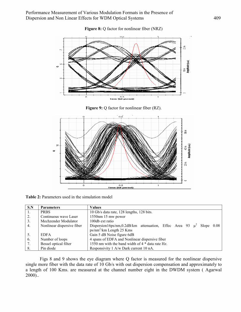
Performance Measurement of Various Modulation Formats in the Presence of Dispersion and Non Linear Effects for WDM Optical Systems 409

Figure 8: Q factor for nonlinear fiber (NRZ)

Figure 9: Q factor for nonlinear fiber (RZ).

Table 2: Parameters used in the simulation model S.N Parameters Values 1. PRBS 10 Gb/s data rate, 128 lengths, 128 bits. 2. Continuous wave Laser 1550nm 15 mw power 3. Mechzender Modulator 100db ext ratio 4. Nonlinear dispersive fiber Dispersion16ps/nm,0.2dB/km attenuation, Effec Area 93 µ2 Slope 0.08

ps/nm2/km Length 25 Kms 5. EDFA Gain 5 dB Noise figure 6dB 6. Number of loops 4 spans of EDFA and Nonlinear dispersive fiber 7. Bessel optical filter 1550 nm with the band width of 4 * data rate Hz. 8. Pin diode Responsivity 1 A/w Dark current 10 nA.

Figs 8 and 9 shows the eye diagram where Q factor is measured for the nonlinear dispersive

single more fiber with the data rate of 10 Gb/s with out dispersion compensation and approximately to a length of 100 Kms. are measured at the channel number eight in the DWDM system ( Agarwal 2000)..

410 A.V.Ramprasad and M.Meenakshi

Results Table 3: comparison of Q factor for RZ and NRZ modulation formats with dispersive and Nonlinear effects

S.N Fiber Type Modulation format Channels Q factor 1. Dispersion compensating NRZ 01 12.753 2. Dispersion compensating RZ 01 16.332 3. Dispersion compensating NRZ 16 7.06 4. Dispersion compensating RZ 16 8.92 5. Dispersion compensating NRZ 32 5.645 6. Dispersion compensating RZ 32 5.567 7. Non linear fiber NRZ 01 7.90 8. Nonlinear fiber RZ 01 15.47

A comparison of various modulation formats for 16 channels DWDM systems are done as

Table 4: Q factor for various modulation formats of Nonlinear fiber. S.N Modulation format Spacings Q factor 1. Return to Zero Equal 1.516 2. Return to Zero Unequal 14. 23 3. Non return to Zero Equal 1.923 4. Non return to Zero Unequal 11.921 5. DPSK Equal 3.15187 6. DPSK Un Equal 18.2323 7. DQPSK Equal 4.2323 8. DQPSK Un Equal 19.999 9. Duobinary Un Equal 20.32 10. RZ duobinary Un equal 22,85

Table 4.shows that Q factor is lower in the case of equal channel spacing this is due to the fact

of FWM effect in the nonlinear dispersive fiber . Discussions In this paper it has been observed that the Q factor can be improved by the modulation scheme either by Return to Zero or Non Return to Zero with the dispersion factor of the transmission medium. Hence in the first half of the paper we have determined an optimal length of the Dispersion compensation fiber to be 120 Kms and for the fixed fiber length we have multiplexed 32 channels and the eye diagram is shown in Figs 5 and 6.Table 3. shows the comparison of RZ and NRZ modulations for two cases with dispersion and non linear effect. It is found that the Q factor for the nonlinear dispersive nature of the fiber for RZ modulation is slightly differed on comparing with the dispersion compensating fiber and conclude that RZ modulations sustain the nonlinearities and dispersive effects than the NRZ modulations Table 4. shows that in the case of equal channel spacing for all the modulation types the Q factor is lower than the Un equal channel spacing this is due to the Non linear effect like Four wave mixing can be suppressed.In the case of 16 DWDM multiplexed channels the modified Duo binary (RZ) format has the highest Q factor in the presence of Non linear effects. Conclusions It was found that the increase in the data rate causes the nonlinear dispersive effects which can be compensated by the compensating fibers and the optimal length of the dispersion compensating length was found and applied to improve the Q factor. It was also observed that by simulation the RZ modulation format can sustain the nonlinear effects at the data rate of 10 Gb/s .On comparing all the

Performance Measurement of Various Modulation Formats in the Presence of Dispersion and Non Linear Effects for WDM Optical Systems 411

major modulation formats it was observed that DPSK and RZ duobinary modulation performs well in the unequal channel spacing systems. References [1] G.P.Agarwal , Non linear optics , 1995 [2] J.Sieben .M,conradi , ‘optical single side band transmission at 10 Gb/s using only electrical

dispersion compensation , Journal of light wave Techology ,IEEE,1999 ,P 1742 [3] A. V. Ramprasad and M.Meenakshi ’A study of ASK and PSK Modulation formats towards

optimal transmission performance in optical communications, Proceedings of International conference on optical networks and communications (ICOCN’05) pp374. Bangkok . Thailand.

[4] A.V.RamPrasad and M.Meenakshi Transmission performance of various modulation formats for nonlinear fiber optic system ”, NCSS 05 A.U. Chennai India June 2005

[5] David R geof ,Chromatic dispersion compensate press Woburn , Massachusetts 2000 [6] G .Bosco and A,Carena ,on the use of NRZ ,RZ and CSRZ modulation formats for UDWM at

40 Gb/s ,in Proc ECOC 2002 paper p 3.7. [7] Anderson and Lyle, Technique for evaluating performance using Q in numerical simulations

exhibiting ISI Electronic letterVol 30, 1994 pp71. [8] G.P.Agarwal, fiber optic communications systems, 2000. [9] I. Morita, K. Tanaka, N. Edagawa, and M. Suzuki, “40 Gbit/s _16 WDM transmission over

2000 km using dispersion managed low-nonlinear fiber span,” in Proc. ECOC’00, Munich, Germany, 2000,.

[10] K. Aikawa, T. Suzuki, T. Suzuki, and A. Wada, “Single-mode optical fiber with effective core area larger than 160 _m ,” in Proc. ECOC’99, Nice, France, 1999, pp. 302–303.

[11] T. Kato, M. Hirano, M. Onishi, and M. Nishimura, “Ultra low nonlinearity low loss pure silica core fiber,” in Proc. OECC’99, Beijing, China, 1999, pp. 1575–1576.

[12] K. Osono, K. Kotani, K. Murakami, Y. Bing, T. Yamazaki, and H. Shimane, “The study of ultra large effective area fiber and mating dispersion slope compensating fiber for dispersion flattened hybrid optical fiber DWDM link,” in Proc. IWCS 2001, Tilburg, The Netherlands, 2001, pp.483–487.

[13] S. N. Knudsen, M. Ø Pedersen, and L. Grüner-Nielsen, “Optimization of dispersion compensating fibers for cabled long-haul applications,” Electron. Lett., vol. 36, pp. 2067–2068, 2000.

[14] O. Y. Takeshita, O. M. Collins, P. C. Massey, and D. J. Costello, “A note on asymmetric turbo-codes,” IEEE Comm. Lett., vol. 3, pp. 69–71, Mar

European Journal of Scientific Research ISSN 1450-216X Vol.15 No.3 (2006), pp. 412-419 © EuroJournals Publishing, Inc. 2006 http://www.eurojournals.com/ejsr.htm

Evaluating the Suitability of Groundcovers in the Arid

Environments of Kuwait

M. Khalil Agriculture and Biodiversity Department

Food Resources and Biological Sciences Division Kuwait Institute for Scientific Research

N. R. Bhat

Agriculture and Biodiversity Department Food Resources and Biological Sciences Division

Kuwait Institute for Scientific Research

M. S. Abdal Agriculture and Biodiversity Department

Food Resources and Biological Sciences Division Kuwait Institute for Scientific Research

R. Grina

Agriculture and Biodiversity Department Food Resources and Biological Sciences Division

Kuwait Institute for Scientific Research

L. Al-Mulla Agriculture and Biodiversity Department

Food Resources and Biological Sciences Division Kuwait Institute for Scientific Research

S. Al-Dossery

Agriculture and Biodiversity Department Food Resources and Biological Sciences Division

Kuwait Institute for Scientific Research

R. Bellen Agriculture and Biodiversity Department

Food Resources and Biological Sciences Division Kuwait Institute for Scientific Research

R. Cruz

Agriculture and Biodiversity Department Food Resources and Biological Sciences Division

Kuwait Institute for Scientific Research

Evaluating the Suitability of Groundcovers in the Arid Environments of Kuwait 413

G. D’Cruz Agriculture and Biodiversity Department

Food Resources and Biological Sciences Division Kuwait Institute for Scientific Research

J. George

Agriculture and Biodiversity Department Food Resources and Biological Sciences Division

Kuwait Institute for Scientific Research

A. Christopher Agriculture and Biodiversity Department

Food Resources and Biological Sciences Division Kuwait Institute for Scientific Research

Abstract

Kuwait is an extremely hot, dry country. Kuwait is an arid country with high. The average daily temperature is about 33°C. Temperatures are even higher during the summer months between May and October, while the humidity is very low. It almost never rains during the summer. Temperatures are more moderate in winter. This is when Kuwait receives its annual rainfall of 25 to 175 millimeters. Sandstorms are common and can last several days. There is very little fresh water in Kuwait. Desalination plants, which distill fresh water from salt water, were built in order to provide the country with enough water. Groundcovers are low growing plants that spread quickly to from a dense cover. These groundcovers are used for reducing the loss of ground water through evaporation. This study was conducted on six ground covers and their performance in the climate of Kuwait was evaluated. It was observed that three out of the six selected ground covers could not withstand the varying temperatures in summer as well as in winter. The plant species like Rhagodia spinescens and Furcraea gigantea showed good growth rate and Allamanda cathartica showed a negative growth rate. The ground covers Hardenbergia comptoniana, Duranta repens goldiana and Lonicera japonica had 0 % survival percentage at the termination of the study. Key Words: Groundcover, desalination, evapo-transpiration, survival percentage, growth

rate Introduction In the arid land of Kuwait we have extreme climatic conditions accompanied by severe sandstorms due to loose structured, sandy nature of the soil. Simultaneously evaporation is very high in Kuwait particularly during summer. At the same time there is a good interest within Kuwait for soil and water conservation and greenery of the country to improve life and the environment (Suleiman and Abdal, 2002). Conservation of both water and soil is an essential concept for Kuwait’s local environment, as water availability, in arid country as Kuwait, is limited and most soils are eroded and native plants are disappearing. Thus it is obvious to control the loss of soil as well as to conserve water. The ground cover plays an important role in conserving the soil and water. Moreover ground covers add beauty to the landscape.

Ground covers are low-growing plants that spread quickly to form a dense cover. They absorb heat, moisture, dust and control erosion. Ground covers vary in form leaf size, color and in texture.

414 M. Khalil, N. R. Bhat, M. S. Abdal, R. Grina, L. Al-Mulla, S. Al-Dossery, R. Bellen, R. Cruz, G. D’Cruz, J. George and A. Christopher

Ground covers can provide a change in foliage structure or add color to landscaped beds. By covering the ground with a carpet of vegetation the ground cover prevents the germination of weeds (Khalil et al., 2006). It acts as an insulating cover for the soil, keeping it cooler in the summer and warmer in the winter. The ground cover is living mulch that helps to build up humus level in the soil. Grass is the best known ground cover, but grass is not suited to all conditions. Other ground cover plants should be used where grass is difficult to grow and maintain. When planted under trees, ground covers reduce the possibility of mower damage to the base of the tree (Relf and Appleton, 1999). Soil erosion models stimulate the reduction in soil loss by incorporating the effect of above ground biomass. But in reality the reduction in soil loss is due to the combined effect of both roots and above ground biomass (Gyssels and Poesen, 2003).

For this study six ground cover species were selected and they were planted in two sites namely, inland site which is away from the vicinity of sea and coastal site near to the sea as the name indicates. They were tested for their growth performance under the harsh climates of Kuwait. Materials and methods Six ground cover species namely Rhagodia spinescens, Allamanda catharicta, Hardenbergia comptoniana, Duranta repens goldiana, Furcraea gigantea and Lonicera japonica were selected for screening for their suitability to Kuwait’s climatic conditions. The land was thoroughly prepared before planting. All weeds, trash, rocks and other debris were cleared and removed from the sites. Chemical analysis of water was also done prior to planting. In both the sites 30 cm of the top layer was back filled with agricultural soil and peat moss. The sites were fine graded and leveled. Soil was disinfected and weed treated. Soil was irrigated before planting to leach salts from the soil and was followed by a drying period of two days. The hardened plants were then transplanted in the field and a complete randomized block design was used. The transplanted plants were medium in size and had a healthy green appearance.

A complete randomized block design with five replications of all experimental plant species in both sites was used. Optimum cultural practices were carried out for the transplanted plants. Ground covers were fertilized with complex fertilizer at the rate of four teaspoons full per square meter area, raked and covered with soil. The lawn area is being maintained by cutting the grass using a lawn mower. The lawn grass is being irrigated with treated-waste-water using the sprinkler irrigation system. Experimental plant species were covered with shade net to protect the plants from high temperature and hot winds. Irrigation water amounts were regulated to meet the plants requirements according to the season. Data on survival, plant height, stem diameter and visual observations were documented on bi-monthly basis. Results and Discussion The means, standard deviation, survival percentages and growth rates were calculated data for the data collected. Table1 shows the survival percentages of the plants in both inland and coastal site, and Fig. 1 is the graphical representation of the same. It was observed that the plant species Hardenbergia comptoniana, Duranta repens goldiana and Lonicera japonica died in the inland site depicting its unsuitability to the harsh weather in Kuwait. Though some of these plants survived in the coastal site, they had very low survival percentages ranging from 20 to 60 %. Rhagodia spinescens and Furcraea gigantea exhibited good survival percentages of 100 % in both the sites. Allamanda cathartica was found to be moderately tolerant to the hot season.

The growth rates of the groundcovers in Table 2 indicate that Rhagodia spinescens had a good growth rates both in the inland and coastal site. In the Coastal site this plant exhibited a growth rate of 272.83 % (Fig. 2). This plant is well adapted for the dry weather condition in prevailing in Kuwait. The growth rate ranged between 40.66-54.61% for the groundcover Furcraea gigantea. Although the plant

Evaluating the Suitability of Groundcovers in the Arid Environments of Kuwait 415

Lonicera japonica survived in the coastal site it had a very low growth rate showing its unsuitability for adaptation in the desert conditions. Table 3 represents the plant caliper of the ground covers. It was observed that among the ground covers the plant Furcraea gigantea has the thickest caliper. It was evident from the Table 4 that Rhagodia spinescens plant exhibited a good plant spread. Table 1 indicates that during the hot season only the plants Rhagodia spinescens and Furcraea gigantean showed excellent growth. During summer the plant Duranta repens goldiana showed drying and burning of the plants. But in winter (Table 6) the plant started developing new shoots and leaves. All these results indicated that the best selected plant for the arid condition is Rhagodia spinescens followed by Furcraea gigantea.

Figure 1: The survival percentages of groundcover plants in the inland and coastal site.

0

20

40

60

80

100

120

Rhag

odia

spin

esce

ns

Alla

man

daca

thar

tica

Har

denb

ergi

aco

mpt

onia

na

Dur

anta

repe

ns

gold

iana

Furc

raea

giga

ntea

Loni

cera

japo

nica

Plant Species

Surv

ival

Per

cent

age

Inland SiteCoastalSite

416 M. Khalil, N. R. Bhat, M. S. Abdal, R. Grina, L. Al-Mulla, S. Al-Dossery, R. Bellen, R. Cruz, G. D’Cruz, J. George and A. Christopher

Figure 2: The growth rate of groundcovers in the inland and coastal site.

-50.00

0.00

50.00

100.00

150.00

200.00

250.00

300.00

Rhag

odia

spin

esce

ns

Alla

man

daca

thar

tica

Har

denb

ergi

aco

mpt

onia

na

Dur

anta

repe

ns

gold

iana

Furc

raea

giga

ntea

Loni

cera

japo

nica

Plant Species

Gro

wth

Rat

e (%

)Inland SiteCoastal Site

Table 1: The Plant Survival of the Groundcovers both in the Inland and Coastal Site

Survival (%) Plant Species Inland Coastal Rhagodia spinescens 100 100 Allamanda cathartica 60 80 Hardenbergia comptoniana 0 0 Duranta repens goldiana 0 20 Furcraea gigantea 100 100 Lonicera japonica 0 60

Evaluating the Suitability of Groundcovers in the Arid Environments of Kuwait 417

Table 2: Mean, Standard Deviation and Growth Rate of Groundcovers in both Inland and Coastal Site

Initial 120 DAP 240 DAP 360 DAP 420 DAP Latin Name Mean (mm)

SD Mean (mm)

SD Mean (mm)

SD Mean SD Mean SD Growth

rate

Inland Rhagodia spinescens 37.20 8.29 78.80 5.81 100.80 6.83 102.00 8.12 100.80 6.83 173.91 Allamanda cathartica 66.80 22.10 62.20 24.43 58.00 42.23 65.67 42.45 58.00 42.23 -6.15 Hardenbergia comptoniana 17.67 7.46 Dead Dead Dead Dead Dead Dead Dead Dead Dead Duranta repens goldiana 18.80 6.30 Dead Dead Dead Dead Dead Dead Dead Dead Dead Furcraea gigantea 31.80 8.23 39.40 5.90 43.60 3.85 42.60 3.78 43.60 3.85 54.61 Lonicera japonica 21.60 5.41 11.00 1.41 Dead Dead Dead Dead Dead Dead Dead Coastal Rhagodia spinescens 36.80 3.70 59.80 4.76 177.80 14.34 135.80 8.11 137.20 6.83 272.83 Allamanda cathartica 61.80 23.85 59.80 26.75 68.25 18.55 74.00 14.12 63.75 15.59 3.16 Hardenbergia comptoniana 7.00 2.00 58.00 39.50 Dead Dead Dead Dead Dead Dead Dead Duranta repens goldiana 18.40 3.65 14.50 3.54 Dead Dead 26.50 3.54 31.00 2.83 68.48 Furcraea gigantea 28.20 0.84 26.80 1.48 32.20 7.73 39.00 5.79 39.67 7.02 40.66 Lonicera japonica 22.60 5.46 24.60 5.55 27.40 4.45 21.67 2.08 20.33 0.58 -10.03

DAP= Days after Planting Table 3: Mean and Standard Deviation of Plant Caliper of the Groundcovers in both Inland and Coastal Site

Initial 120 DAP 240 DAP 360 DAP 420 DAP Latin Name Mean (mm)

SD Mean (mm)

SD Mean (mm)

SD Mean SD Mean (mm)

SD

Inland Rhagodia spinescens 4.20 0.45 6.00 0.00 10.20 1.30 19.00 1.22 19.40 1.14 Allamanda cathartica 4.40 0.55 6.20 0.45 6.20 0.45 7.33 0.58 7.33 0.58 Hardenbergia comptoniana 2.00 0.00 2.33 0.58 Dead Dead Dead Dead Dead Dead Duranta repens goldiana 2.80 0.84 4.67 0.58 5.00 0.00 Dead Dead Dead Dead Furcraea gigantea 41.50 7.23 41.60 7.23 45.20 5.54 47.40 5.22 47.60 4.83 Lonicera japonica 3.20 0.45 4.20 0.45 6.20 0.84 Dead Dead Dead Dead Coastal Rhagodia spinescens 4.00 0.00 6.40 1.14 16.40 0.55 21.00 0.71 21.60 1.14 Allamanda cathartica 5.20 1.30 6.20 1.10 6.50 1.00 8.25 0.96 8.25 0.96 Hardenbergia comptoniana 2.00 0.00 2.00 0.00 Dead Dead Dead Dead Dead Dead Duranta repens goldiana 5.20 1.30 5.00 1.41 Dead Dead 8.00 1.41 9.00 1.41 Furcraea gigantea 29.00 4.80 29.00 4.80 36.20 3.90 48.60 6.19 50.67 5.51 Lonicera japonica 4.20 1.79 4.60 1.34 22.20 32.35 8.33 1.53 8.33 1.53

DAP= Days after Planting

418 M. Khalil, N. R. Bhat, M. S. Abdal, R. Grina, L. Al-Mulla, S. Al-Dossery, R. Bellen, R. Cruz, G. D’Cruz, J. George and A. Christopher

Table 4: Mean and Standard Deviation of Plant Cover of the Groundcovers in both Inland and Coastal Site

90 DAP 180 DAP 240 DAP 360 DAP 420 DAP Latin Name Mean (mm)

SD Mean (mm)

SD Mean (mm)

SD Mean SD Mean SD

Inland Rhagodia spinescens 22.40 2.30 65.40 6.11 70.20 6.98 117.60 12.42 119.80 12.79 Allamanda cathartica 12.00 1.22 9.40 4.98 16.60 13.94 21.00 24.76 17.33 24.85 Hardenbergia comptoniana

13.67 4.73 23.00 0.00 Dead Dead Dead Dead Dead Dead

Duranta repens goldiana 9.67 4.93 10.00 0.00 14.00 0.00 Dead Dead Dead Dead Furcraea gigantea 35.80 5.07 37.40 4.83 35.00 3.87 43.60 2.88 45.40 2.30 Lonicera japonica 27.20 4.92 39.80 1.64 49.20 4.92 Dead Dead Dead Dead Coastal Rhagodia spinescens 63.40 7.27 137.80 137.80 199.20 12.44 180.40 8.08 180.60 8.65 Allamanda cathartica 12.80 3.90 15.20 15.20 33.25 17.50 40.75 16.42 32.00 10.74 Hardenbergia comptoniana

20.00 7.52 32.40 32.40 Dead Dead Dead Dead Dead Dead

Duranta repens goldiana 18.00 4.24 14.00 14.00 Dead Dead 35.50 3.54 36.00 5.66 Furcraea gigantea 34.20 3.05 34.20 34.20 37.60 7.02 49.00 7.97 54.00 8.72 Lonicera japonica 24.80 4.87 53.20 53.20 59.40 4.34 28.00 6.00 28.33 3.79

DAP= Days after Planting Table 5: The effect of High Temperature on the Growth and Nature of the Experimental Plant Name of plant Effects of High Temperature Rhagodia spinescens Excellent growth. Increase in the size of the plant. Flowers still remain in the plant. Allamanda cathartica The tips of leaves dried. Leaves show acute chlorosis. The main stem turned to pale red.

The leaves of the plant show curling towards inner side. Harenbergia comptoniana Total drying of plants. The tip of the branches first dried and later it spread to the base. Duranta repens goldiana Drying and burning of plants were noticed. Furcraea gigantea New healthy shoots are coming. Excellent growth. The increase in size of collar region

shows its healthy nature. Lonicera japonica The tips of leaves were dried. The prostrate branches running in the ground were

completely dried, leading to decrease in plant cover. Increase in size of leaves. Table 6: The effect of Low Temperature on the Growth and Nature of the Experimental Plant Name of plant Effects of High Temperature Rhagodia spinescens Excellent growth. Good, extensive growth of foliage gives the plant a bushy appearance.

The plants produced flowers. Allamanda catharicta Plants showed loss of vigor. The growing part was dried from top downwards. Leaves

from the upper part were dried and shredded. Hardenbergia comptoniana Total loss due to high temperature in summer. Duranta repens goldiana Excellent growth. The leaves were well developed and showed characteristic golden

yellow color. Formations of lateral branches lead to development of more luxurious leaves.

Furcraea gigantea Very good growth. No effect of cold on the growth and development. Increase in size of the collar region as well as the size of leaves were noticed.

Lonicera japonica Dried lateral branches. As the season progressed, the newly formed leaves showed drying and shredding.

Acknowledgement The project team would like to thank the Kuwait Foundation for the Advancement of Sciences for their financial support of the study; as well as the management of the Kuwait Institute for Scientific Research for their continued support and interest in the project.

Evaluating the Suitability of Groundcovers in the Arid Environments of Kuwait 419

References [1] Gyssels, G. and J. Poesen. 2003 The importance of plant root characteristics in controlling

concentrated flow erosion rates. Earth Surface Processes and Landforms. 28: 371-384. [2] Khalil, M., N.R. Bhat, L.A. Al-Mulla, S. Al-Dossery, R. Bellen, M. Al-Zalzalah, G. D’Cruz

and R. Cruz. 2006. Evaluation of new ornamental plants for use in Kuwait’s landscape and demonstration gardens establishment (FA024C). Kuwait Institute for Scientific Research, Progress Report No. V. KISR 8084, Kuwait.

[3] Suleiman M. K. and M. S. Abdal. 2002. Water availability for the greening of Kuwait. 2002. Limnologica - Ecology and Management of Inland Waters. Volume 32(4) pp. 322-328.

[4] Relf, D. and B. Appleton. 1999. Selecting landscape plants; groundcovers. Environmental Horticulture. Virginia Cooperative Extension, Publication 426-609.

European Journal of Scientific Research ISSN 1450-216X Vol.15 No.3 (2006), pp. 420-426 © EuroJournals Publishing, Inc. 2006 http://www.eurojournals.com/ejsr.htm

Evaluation and Screening of Suitable Vines for the Arid

Conditions of Kuwait

M. K. Suleiman Agriculture and Biodiversity Department

Food Resources and Biological Sciences Division Kuwait Institute for Scientific Research

N. R. Bhat

Agriculture and Biodiversity Department Food Resources and Biological Sciences Division

Kuwait Institute for Scientific Research

M. S. Abdal Agriculture and Biodiversity Department

Food Resources and Biological Sciences Division Kuwait Institute for Scientific Research

L. Al-Mulla

Agriculture and Biodiversity Department Food Resources and Biological Sciences Division

Kuwait Institute for Scientific Research

R. Grina Agriculture and Biodiversity Department

Food Resources and Biological Sciences Division Kuwait Institute for Scientific Research

S. Al-Dossery

Agriculture and Biodiversity Department Food Resources and Biological Sciences Division

Kuwait Institute for Scientific Research

R. Bellen Agriculture and Biodiversity Department

Food Resources and Biological Sciences Division Kuwait Institute for Scientific Research

R. Cruz

Agriculture and Biodiversity Department Food Resources and Biological Sciences Division

Kuwait Institute for Scientific Research

Evaluation and Screening of Suitable Vines for the Arid Conditions of Kuwait 421

G. D’Cruz Agriculture and Biodiversity Department

Food Resources and Biological Sciences Division Kuwait Institute for Scientific Research

J. George

Agriculture and Biodiversity Department Food Resources and Biological Sciences Division

Kuwait Institute for Scientific Research

A. Christopher Agriculture and Biodiversity Department

Food Resources and Biological Sciences Division Kuwait Institute for Scientific Research

Abstract

Vines offer an interesting variation in plant form. They are valuable in the landscape for their practical and aesthetic qualities. If vines are to be satisfactory in the landscape, they must be well adapted to the environment in which they are to be grown. Especially in Kuwait, where the atmospheric temperature is too high during the months of June to August and frost and cold winds during the winter months, it is important to adapt the suitable vines that are compatible with other components of landscapes. With this view in mind a study was initiated on eight species of vines namely, Clematis microphylla, Clerodendrum thomsoniae, Cryptostegia grandiflora, Ficus pumila, Hardenbergia violacea, Ipomoea horsfalliae, Pandorea jasminoides, and Petrea volubilis were tested in the inland and coastal sites. These vines were subjected to the arid climates of Kuwait and evaluated for their suitability. It was observed that the except Cryptostegia grandiflora, all other vines species were susceptible to the harsh weather prevailed during the summer in Kuwait. Four vine species had 0 % survival percentage. Ipomoea horsfalliae and Petrea volubilis exhibited a negative growth rate and Pandorea jasminoides was found to have a slow growth rate. Keywords: Vines, landscape, aesthetic quality, frost, harsh weather, survival percentage,

growth rate. Introduction Kuwait is an arid country with harsh climate, where the temperature means range from 8o to 44o in January and July respectively. The soil is sandy in texture. To ensure successful landscape, one should consider the type of soil, water quality and availability. Desert soil in general are short of organic matter, sandy with sparse vegetation, low in nitrogen, low in phosphorus, alkaline due to high content of calcium and often contains sodium (Khalil et al, 2003). The selection of plants best suited to these types of soils and climate is an important criteria. Along with trees, shrubs and ground cover, vine is also an important component of landscape gardening.

Vines include all plants, whether woody or herbaceous, that requires some support for their development. Vines are versatile and can grow quickly as a groundcover, a screen in trellis, a cascade of foliage and flowers against a wall, a leafy cover on an arbor, or a climber on a wall or a tree (Harris, 1992). Vines can form excellent screen plants for fences, and add appeal when grown on trees or shrubs. Combined with overhead structure, vines can provide delightful shade areas. They also perform

422 M. K. Suleiman, N. R. Bhat, M. S. Abdal, L. Al-Mulla, R. Grina, S. Al-Dossery, R. Bellen, R. Cruz, G. D’Cruz, J. George and A. Christophe

well as windbreaks. There are annual and perennial vines, woody and herbaceous vines, evergreen and deciduous vine, flowering vines and vines grown primarily for their foliage. We may use vines in several ways. They include using on walls or other overhead structures and as groundcovers. The trees, shrubs and vines have some effects on the space cooling requirements of a building in a warm humid environment (Parker, 1981).

The study was conducted in the urban demonstration garden in Kuwait (coastal site) and in a commercial garden (inland site). The eight species of vines listed in Table 1 were tested for their suitability to the harsh climates of Kuwait was evaluated. These plants were imported from Australia and India. The plant species were known to survive under similar climatic conditions in their respective countries. Materials and Methods Eight vines namely, Clematis microphylla, Clerodendrum thomsoniae, Cryptostegia grandiflora, Ficus pumila, Hardenbergia violacea, Ipomoea horsfalliae, Pandorea jasminoides, and Petrea volubilis were selected for screening for their suitability to Kuwait’s climatic conditions. The land was thoroughly prepared before planting. All weeds, trash, rocks and other debris were cleared and removed from the sites. Chemical analysis of water was also done prior to planting. 30 cm of the top layer was back filled with agricultural soil and peat moss. The sites were fine graded and leveled. Soil was disinfected and weed treated. Soil was irrigated before planting to leach salts from the soil and was followed by a drying period of two days. The plants after were allowed to harden in the greenhouses before planting in the field. The hardened plants were then transplanted in the field and a complete randomized block design was used. The transplanted plants were medium in size and had a healthy green appearance.

A complete randomized block design with five replications of all experimental plant species in both sites was used. Optimum cultural practices were carried out for the transplanted plants. The vines were trailed on the supports such as fence, bamboo stalks and tied. The unwanted and dried branches were removed. Experimental plant species were covered with shade net to protect the plants from high temperature and hot winds. Irrigation water amounts were regulated to meet the plants requirements according to the season. Data on survival, plant height, stem diameter and visual observations were documented on bi-monthly basis. Results and Discussion The data on plant height, plant girth, plant canopy and other visual observations were tabulated and their mean and standard deviation were calculated. It was observed that the vine Cryptostegia grandiflora showed hundred percent survivals both in the inland and coastal site (Table 1). Ipomea horsfalliae also showed about 40 % survival in the inland site. All other plant species died indicating their unsuitability to Kuwait’s weather. In the coastal site the plants Ipomea horsfalliae and Pandorea jasminoides showed cent percent survival. Clematis microphylla, Clerodendrum thomsoniae and Hardenbergia violacea died in the coastal site. A graphical representation of the survival percentages of the vines are presented in Fig 1.

Table 2 indicates the mean plant height, standard deviation and growth rate of the vines in the inland and in the coastal site. The vine Cryptostegia grandiflora exhibited the highest growth rate of 178.90% and 213.76% in the inland and coastal site respectively (Fig 2).In the inland site the species Ipomea horsfalliae showed negative growth rate. All other plants died in this site due to the extreme heat in summer.The vine species Ipomoea horsfalliae and Petrea volubilis exhibited negative growth rate in the costal site. Pandorea jasminoides showed very slow growth rate in summer. Table 3 represents the plant caliper and table 4 is the plant canopy of the experimental plants in both sites. The effect of temperature on the growth and development of the vines are indicated in Table 5 and 6.

Evaluation and Screening of Suitable Vines for the Arid Conditions of Kuwait 423

Table 1: The Survival Percentages of Vines in the Coastal Site and Inland Site

Plant Species Inland Site Coastal Site Clematis microphylla 0 0 Clerodendrum thomsoniae 0 0 Cryptostegia grandiflora 100 100 Ficus pumila 0 40 Hardenbergia violacea 0 0 Ipomea horsfalliae 40 100 Pandorea jasminoides 0 100 Petrea volubilis 0 40

Table 2: Mean, Standard Deviation and Growth Rate of Vines in the Inland and Coastal Site

Initial 120 DAP 240 DAP 360 DAP 420 DAP Growth rate

Mean SD Mean SD Mean SD Mean SD Mean SD Inland Site Clematis microphylla 13.40 4.67 17.00 14.28 Dead Dead Dead Dead Dead Dead Dead Clerodendrum thomsoniae 27.80 12.54 33.20 9.44 17.50 7.78 Dead Dead Dead Dead Dead Cryptostegia grandiflora 79.20 10.57 85.40 10.57 162.20 41.17 182.80 25.81 182.40 25.24 178.90 Ficus pumila 15.00 9.27 32.50 17.68 40.00 0.00 Dead Dead Dead Dead Dead Hardenbergia violacea 26.40 10.88 43.60 10.01 Dead Dead Dead Dead Dead Dead Dead Ipomea horsfalliae 60.60 36.15 48.60 37.13 76.75 78.64 Dead Dead 22.00 1.41 -46.60 Pandorea jasminoides 14.20 5.50 24.50 23.33 62.50 43.13 Dead Dead Dead Dead Dead Petrea volubilis 40.60 6.88 46.67 14.22 50.50 13.44 Dead Dead Dead Dead Dead Coastal Site Clematis microphylla 17.60 9.32 138.20 48.39 10.80 4.60 Dead Dead Dead Dead Dead Clerodendrum thomsoniae 22.40 9.71 27.20 10.83 Dead Dead Dead Dead Dead Dead Dead Cryptostegia grandiflora 65.40 7.13 91.80 11.34 191.20 71.91 231.20 65.17 205.20 59.81 213.76 Ficus pumila 7.00 1.41 14.80 4.97 19.00 4.64 Dead Dead Dead Dead Dead Hardenbergia violacea 39.60 16.74 63.80 22.08 Dead Dead Dead Dead Dead Dead Dead Ipomoea horsfalliae 41.20 65.34 17.40 5.32 105.40 64.64 17.00 7.81 14.50 7.78 -64.81 Pandorea jasminoides 42.40 21.52 44.40 13.90 70.40 59.63 52.60 15.50 56.25 8.10 32.67 Petrea volubilis 43.20 15.17 48.60 18.51 46.00 17.05 32.00 19.80 31.50 21.92 -27.08

DAP= Days after Planting, SD= Standard Deviation, Growth rate= Final Height-Initial Height x 100 Initial Height

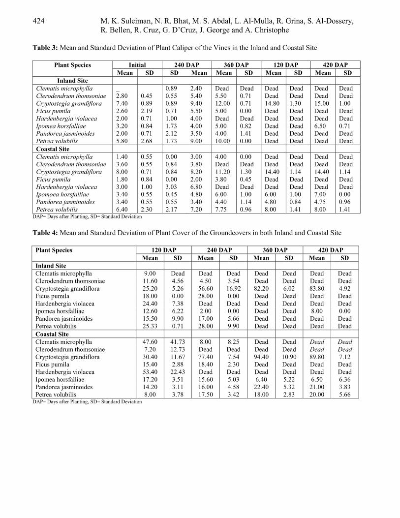
424 M. K. Suleiman, N. R. Bhat, M. S. Abdal, L. Al-Mulla, R. Grina, S. Al-Dossery, R. Bellen, R. Cruz, G. D’Cruz, J. George and A. Christophe

Table 3: Mean and Standard Deviation of Plant Caliper of the Vines in the Inland and Coastal Site

Initial 240 DAP 360 DAP 120 DAP 420 DAP Plant Species Mean SD SD Mean Mean SD Mean SD Mean SD

Inland Site Clematis microphylla _ 0.89 2.40 Dead Dead Dead Dead Dead Dead Clerodendrum thomsoniae 2.80 0.45 0.55 5.40 5.50 0.71 Dead Dead Dead Dead Cryptostegia grandiflora 7.40 0.89 0.89 9.40 12.00 0.71 14.80 1.30 15.00 1.00 Ficus pumila 2.60 2.19 0.71 5.50 5.00 0.00 Dead Dead Dead Dead Hardenbergia violacea 2.00 0.71 1.00 4.00 Dead Dead Dead Dead Dead Dead Ipomea horsfalliae 3.20 0.84 1.73 4.00 5.00 0.82 Dead Dead 6.50 0.71 Pandorea jasminoides 2.00 0.71 2.12 3.50 4.00 1.41 Dead Dead Dead Dead Petrea volubilis 5.80 2.68 1.73 9.00 10.00 0.00 Dead Dead Dead Dead Coastal Site Clematis microphylla 1.40 0.55 0.00 3.00 4.00 0.00 Dead Dead Dead Dead Clerodendrum thomsoniae 3.60 0.55 0.84 3.80 Dead Dead Dead Dead Dead Dead Cryptostegia grandiflora 8.00 0.71 0.84 8.20 11.20 1.30 14.40 1.14 14.40 1.14 Ficus pumila 1.80 0.84 0.00 2.00 3.80 0.45 Dead Dead Dead Dead Hardenbergia violacea 3.00 1.00 3.03 6.80 Dead Dead Dead Dead Dead Dead Ipomoea horsfalliae 3.40 0.55 0.45 4.80 6.00 1.00 6.00 1.00 7.00 0.00 Pandorea jasminoides 3.40 0.55 0.55 3.40 4.40 1.14 4.80 0.84 4.75 0.96 Petrea volubilis 6.40 2.30 2.17 7.20 7.75 0.96 8.00 1.41 8.00 1.41

DAP= Days after Planting, SD= Standard Deviation Table 4: Mean and Standard Deviation of Plant Cover of the Groundcovers in both Inland and Coastal Site

120 DAP 240 DAP 360 DAP 420 DAP Plant Species Mean SD Mean SD Mean SD Mean SD

Inland Site Clematis microphylla 9.00 Dead Dead Dead Dead Dead Dead Dead Clerodendrum thomsoniae 11.60 4.56 4.50 3.54 Dead Dead Dead Dead Cryptostegia grandiflora 25.20 5.26 56.60 16.92 82.20 6.02 83.80 4.92 Ficus pumila 18.00 0.00 28.00 0.00 Dead Dead Dead Dead Hardenbergia violacea 24.40 7.38 Dead Dead Dead Dead Dead Dead Ipomea horsfalliae 12.60 6.22 2.00 0.00 Dead Dead 8.00 0.00 Pandorea jasminoides 15.50 9.90 17.00 5.66 Dead Dead Dead Dead Petrea volubilis 25.33 0.71 28.00 9.90 Dead Dead Dead Dead Coastal Site Clematis microphylla 47.60 41.73 8.00 8.25 Dead Dead Dead Dead Clerodendrum thomsoniae 7.20 12.73 Dead Dead Dead Dead Dead Dead Cryptostegia grandiflora 30.40 11.67 77.40 7.54 94.40 10.90 89.80 7.12 Ficus pumila 15.40 2.88 18.40 2.30 Dead Dead Dead Dead Hardenbergia violacea 53.40 22.43 Dead Dead Dead Dead Dead Dead Ipomea horsfalliae 17.20 3.51 15.60 5.03 6.40 5.22 6.50 6.36 Pandorea jasminoides 14.20 3.11 16.00 4.58 22.40 5.32 21.00 3.83 Petrea volubilis 8.00 3.78 17.50 3.42 18.00 2.83 20.00 5.66

DAP= Days after Planting, SD= Standard Deviation

Evaluation and Screening of Suitable Vines for the Arid Conditions of Kuwait 425

Figure 1: The survival percentages of groundcover plants in the inland and coastal site.

0

20

40

60

80

100

120

Cle

mat

ism

icro

phyl

la

Cle

rode

ndru

mth

omso

niae

Cry

ptos

tegi

agr

andi

flora

Ficu

s pum

ila

Har

denb

ergi

avi

olac

ea

Ipom

eaho

rsfa

lliae

Pand

orea

jasm

inoi

des

Petr

eavo

lubi

lis

Plant Species

Surv

ival

(%)

Inland SiteCoastalSite

Figure 2: The growth rate of groundcovers in the inland and coastal site.

-100.00

-50.00

0.00

50.00

100.00

150.00

200.00

250.00

Cle

mat

ism

icro

phyl

la

Cle

rode

ndru

mth

omso

niae

Cry

ptos

tegi

agr

andi

flora

Ficu

s pum

ila

Har

denb

ergi

avi

olac

ea

Ipom

eaho

rsfa

lliae

Pand

orea

jasm

inoi

des

Petr

eavo

lubi

lis

Plant Species

Gro

wth

Rat

e (%

)

Inland SiteCoastal Site

426 M. K. Suleiman, N. R. Bhat, M. S. Abdal, L. Al-Mulla, R. Grina, S. Al-Dossery, R. Bellen, R. Cruz, G. D’Cruz, J. George and A. Christophe

Table 5: Effect of High Temperature on the Growth and Nature of Original Experimental Plants

Plant Species Effects of Low Temperature Clematis microphylla Total drying of plants due to excess heat. Could not with stand high temperature for

continuous periods. Clerodendrum thomsoniae Total loss of plants. Cryptostegia grandiflora Excellent growth. More branches from all parts of main stem, which are trailing actively.

Elongation of the inter-nodal region leads to increase in height of plants. The branches were growing at a faster rate than the main stem.

Ficus pumila No growth. Total drying of leaves and branches. Hardenbergia violacea After a luxurious growth, plants were dead due to high temperature. The leaves first turn to

pale green and then complete drying. Ipomoea horsfalliae Total drying of the leaves, but the vines remained healthy. The drying of vines starts from

the tips leading to decrease in plant cover. But new growths can be seen from leaf axils. Pandorea jasminoides Not much effect. Drying of leaves can be seen. Petrea volubilis Drying can be seen on the margins of the leaves. New growth can be seen on stem axils.

The plants lost their vigor and health. Table 6: Effect of Low Temperature on the Growth and Nature of Original Experimental Plants

Plant Species Effects of Low Temperature Clematis microphylla Total loss during summer. Clerodendrum thomsoniae Total loss of plants. Cryptostegia grandiflora Shredding of leaves from main stem. Healthy shoots were coming from the base. Upper

part of the main stem was dried. New leaves were very healthy. Ficus pumila Total loss during summer. Hardenbergia violacea Total loss during summer due to high temperature. Ipomoea horsfalliae The wine length was reduced substantially due to the drying of wines. The leaves were

dried. Pandorea jasminoides Almost retarded growth. The leaves showed chlorosis. The wine length was reduced. Petrea volubilis Good growth. New leaves were coming.

Acknowledgement The project team would like to thank the Kuwait Foundation for the Advancement of Sciences for their financial support of the study; as well as the management of the Kuwait Institute for Scientific Research for their continued support and interest in the project. References [1] Khalil, M. and R.H. Grina. 2003. Evaluation of new ornamental plants for use in Kuwait’s

landscape and demonstration gardens establishment. Proposal KISR 6759 [2] Harris, R. W. 1992. Arboriculture: Integrated management of landscape trees shrubs and vines.

2nd edition. Prentice Hall Incorporated, Englewood Cliffs, New Jersey [3] Parker, J.H. 1982. Landscape elements and climate parameters in energy conservation design.

Proceedings of American Society of Forestry. Pp: 364-368

View publication statsView publication stats