european summe r sym posium in financia l … - firm characteristics... · associated with the...

F

Leo

Th

EURO

Firm C

onid Kog

The views exporgani

PEAN S

Charac

an (MIT S

pressed in thisation(s), no

SUMME

cteristDat

Sloan Sc

his paper areor of CEPR, w

ER SYM

GenerStudy C

Monday

tics ana-Mini

chool of M

e those of thewhich takes

MPOSIU

rously hosCenter Ger

y 15-26 Ju

nd Eming Ex

Managem

Board)

e author(s) anno institution

M IN FI

sted by rzensee

uly 2013

piricaxperim

ment) and

nd not thosenal policy pos

NANCIA

l Factoment

*Mary Ti

e of the fundinsitions.

AL MAR

or Mod

ian (Fede

ng

RKETS

dels: a

eral Rese

a

erve

Firm Characteristics and Empirical Factor Models: aData-Mining Experiment∗

Leonid Kogan †

Mary Tian ‡

June 2013

Abstract

“A three-factor model using the momentum and cashflow-to-price factors explains 14well-known asset pricing anomalies.” Our data-mining experiment provides a backdropagainst which such claims can be evaluated. We construct three-factor linear pricingmodels that match return spreads associated with as many as 14 out of 27 commonlyused firm characteristics over the 1971-2011 sample. We form target assets by sortingfirms into ten portfolios on each of the chosen characteristics and form candidate pricingfactors as long-short positions in the extreme decile portfolios. Our analysis exhaustsall possible 351 three-factor models, consisting of two characteristic-based factors inaddition to the market portfolio. 71% and 48% of the examined factor models matcha larger fraction of the target return cross-sections than the CAPM or the Fama-French three-factor model, respectively. We find that the relative performance of thecomplete set of three-factor models is highly sensitive to the sample choice and thefactor construction methodology. Our results highlight the challenges of evaluatingempirical factor models.

Keywords: Anomalies, Factor Model, Data-mining, Firm Characteristic

JEL Classification: G12

∗We thank seminar participants at the Finance Forum workshop at the Federal Reserve Board of Gov-ernors. The views in this paper are solely the responsibility of the authors and should not be interpretedas reflecting the views of the Board of Governors of the Federal Reserve System or of any other personassociated with the Federal Reserve System.

†NBER and MIT Sloan School of Management, [email protected].

‡Division of International Finance, Federal Reserve Board of Governors, [email protected].

1 Introduction

Empirical asset pricing literature has documented many examples of firm characteristics

being able to predict future stock returns. When not accounted for by standard asset pric-

ing models, such patterns are often interpreted as anomalous. It is challenging to develop

meaningful theoretical explanations of the observed patterns in returns.1 In contrast, the

long-short portfolios constructed by sorting firms on various characteristics – the “c-factors”,

often named after the sorting variable – provide readily available inputs into empirical factor

models. By searching through the firm characteristics known to be associated with large

spreads in stock returns, it is relatively easy to construct seemingly successful empirical

factor pricing models.

When we hear of a new c-factor model withN factors that “explains”M of the well-known

anomalies, how should we evaluate such a result? Is there a quantitative threshold for the M -

to-N ratio, above which such a result strongly points to an economically important source

of systematic risk, even without a solid theoretical foundation? The ease of construction

of c-factor models and virtually unlimited freedom in selecting test assets provide fertile

ground for data mining.2 In this paper we quantify just how easy it is to generate seemingly

successful empirical c-factor models. Our findings imply that it is extremely difficult to

evaluate factor pricing models based solely on their pricing performance, and one must

emphasize the theoretical and empirical foundation for their economic mechanism.

We systematically data-mine the 1971-2011 historical sample under a specific set of rules

designed to be representative of commonly used empirical procedures. We consider 27 firm

characteristics proposed in the literature as predictive variables for stock returns (see section

2 and Appendix A for the list of the characteristics, with references to the relevant litera-

1“Meaningful” is an important qualifier here: it is not difficult to come up with an ad hoc ex-post ra-tionalization of why a particular firm characteristic may proxy for exposure to a risk factor. A compellingtheoretical explanation should identify the economic mechanism giving rise to such a factor, provide alter-native testable implications of this mechanism, and contain a rationale for why other firm characteristics arecorrelated with firms’ exposures to the proposed risk factor.

2Many studies in the literature warn of the dangers of data mining biases, particularly in the contextof return predictability, e.g., Black (1993), Lo and MacKinlay (1990), Ferson (1996), Lewellen, Nagel, andShanken (2010), Novy-Marx (2012).

1

ture). Some of these characteristics have been proposed as candidate empirical proxies for

systematic risk exposures, others as likely proxies for mispricing. A firm characteristic simply

needs to be a subject of an academic publication in order to be included in our data-mining

exercise.

We rank firms into ten portfolios based on each of the 27 characteristics and define the

associated return factors as return differences between the tenth and the first decile portfolios.

We then tabulate the pricing performance of all possible three- and four-factor models, each

consisting of the market portfolio and two or three factors respectively, chosen out of the set

of 27. We thus consider a total of 351 alternative three-factor models, and 2,925 four-factor

models.

If a pricing model is not rejected by testing it against a cross-section of portfolios sorted

on a particular firm characteristic, we say that this model matches such a cross-section. We

find that it is relatively easy to construct a three-factor model that match more than half

of the 25 target cross-sections of returns over the full sample (we exclude the cross-sections

used to form the model factors from the set of target cross-sections).

The best-performing model over the entire sample, by the total number of matched

cross-sections, includes the factors based on momentum and the cash flow-to-price ratio.

It matches 14 out of 25 return cross-sections. Each of the top-twenty models reported in

Table 5 matches return cross-sections based on each of 11 or more different characteristics.3

Four-factor models achieve slightly better coverage, with the top model matching 14 out of

24 cross-sections, and the worst of the top-twenty models matching 13. For comparison, the

CAPM and the Fama and French (1993) three-factor model match seven and eight out of 27

return cross-sections, respectively (we do not exclude any test assets when evaluating these

reference models).

As expected in a data mining exercise, performance of the c-factor models tends to be

fragile. It is highly sensitive to the sample period choice and the details of the factor construc-

tion. In particular, there is virtually no correlation between the relative model performance

3We summarize performance of all 351 models in an on-line document, http://tinyurl.com/d43mf3h.

2

http://tinyurl.com/d43mf3h

in the first and the second halves of the 1971-2011 sample period. Likewise, using a two-way

sort on firm stock market capitalization (size) and characteristics to construct model return

factors, an often used empirical procedure, similarly scrambles the relative model rankings.

Such lack of stability suggests that our data-snooping algorithm tends to pick spurious win-

ners among the set of all possible models without revealing a robust underlying risk structure

in returns. This does not mean that all of the better-performing models in our analysis are

spurious and theoretically unjustifiable. Some of the many models we enumerate in this

study are likely to capture economically meaningful sources of risk – we just cannot identify

which of them do, based solely on the models’ pricing performance.

This paper is organized as follows. Section 2 describes the data and methodology. Sec-

tion 3 examines the overall factor structure of characteristic-sorted portfolios and the abil-

ity of c-factor models to capture cross-sectional differences in average returns on various

characteristic-sorted portfolios. Section 4 concludes.

2 Data and Methodology

In this section, we describe the data used in our analysis and our empirical methodology.

Data on annual and quarterly firm fundamentals are from Compustat. Monthly data on

firm-level stock returns, shares outstanding, and volume are from the Center for Research

in Security Prices (CRSP) database. Aggregate market liquidity data are from Pastor and

Stambaugh (2003). Our sample period is 1971-2011, with subsample periods 1971-1991 and

1992-2011.

We consider a total of 27 firm characteristics, which we informally partition into seven

groups:

1. valuation: size (SIZE), book-to-market (BM), dividend-to-price (DP), earnings-to-

price (EP), cash flow-to-price (CP);

2. investment: investment-to-assets (IA), asset growth (AG), accruals (AC), abnormal

investment(AI), net operating assets (NOA), investment-to-capital (IK), investment

3

growth (IG);

3. prior returns: momentum (MOM), long-term reversal (LTR);

4. earnings: return on assets (ROA), standardized unexpected earnings (SUE), return on

equity (ROE), sales growth (SG);

5. financial distress: Ohlson score (OS), market leverage (LEV);

6. external financing: net stock issues (NSI), composite issuance (CI);

7. other: organization capital (OK), liquidity risk (LIQ), turnover (TO), idiosyncratic

return volatility (VOL), market beta (BETA).4

The definitions and construction of the characteristics are contained in Appendix A.

After dropping all firms in the financial sector (SIC 6000-6999), we sort remaining firms

into ten portfolios with respect to each characteristic, thus performing 27 independent one-

way sorts. We sort firms every year in June with respect to the underlying characteristic

and then compute value-weighted returns of each portfolio from July to June of the next

year.5 We take the difference in value-weighted returns of the high and low portfolios (decile

10 minus decile 1) to form 27 characteristic return factors.6 Alternatively, we also construct

factors by doing a sequential double-sort on size and then the characteristic: firms are

separated into either big or small firms, and subsequently within each group, sorted into ten

portfolios with respect to the characteristic. Then, we construct each factor as the equal-

weighted average of the high minus low portfolio within the big and small size group. Our

4Strictly speaking, market beta is a measure of risk, and is not what is typically taken as a firm charac-teristic. We include market beta as one of the sorting variables because of the recent resurgence of interestin the failure of CAPM to price the market-beta sorted portfolios (e.g., Black, Jensen, and Scholes, 1972;Frazzini and Pedersen, 2011; Baker, Bradley, and Wurgler, 2011). Similarly, idiosyncratic return volatilityis a return statistic rather than a firm characteristic observable at a point in time. We include idiosyncraticvolatility because of its striking ability to forecast future stock returns, e.g., Ang, Hodrick, Xing, and Zhang(2006).

5The following are exceptions: following the original papers, we sort monthly on idiosyncratic volatility,market beta, momentum, long-term reversal, and turnover, and compute value-weighted returns for thefollowing month. We sort on liquidity beta at the end of every December and compute returns for thefollowing calendar year, following Pastor and Stambaugh (2003).

6 In particular, to be consistent, we construct the size and book-to-market factors in this manner, whichwe call SIZE and BM , instead of using the standard Fama-French factors SMB and HML.

4

base set of results use factors constructed from the one-way sort; we compare results using

the alternative double-sort factor construction in Section 3.3.

We create three-factor models by taking the market portfolio and choosing two factors

among our 27 return factors. Overall, this generates a universe of 351 linear three-factor

models. In addition to the complete list of all possible three-factor empirical models, we

also consider the CAPM; the Fama-French three-factor model; and a model consisting of

the market portfolio and the first two principal component vectors from the span of the 27

factor returns. While CAPM is perhaps the most commonly used theoretical benchmark,

the other two models are empirical factor models.

We test each factor model’s ability to match the average return differences across port-

folios sorted on each characteristic using a standard time-series regression framework. In

particular, following Gibbons, Ross, and Shanken (1989), for each characteristic we regress

excess returns on the ten characteristic-sorted portfolios on the returns of the three factors:

rin − rf = αi + βin,MKT (rMKT − rf ) + βin,jrj + βin,krk + εin, (1)

where i = 1, ..., 10 indexes the decile portfolios sorted on the characteristic number n, n =

1, ..., 27; j and k are the c-factors formed on characteristics j and k respectively, j < k. We

perform the Gibbons et al. (1989) F-test of the hypothesis that α1 = α2 = · · · = α10 = 0.

We say that a three-factor model using c-factors j and k is able to match, or capture, the

cross-section of returns on portfolios sorted on characteristic n if the p-value of the F-test,

pFn,j,k, exceeds ten percent.

For each three-factor model, we exclude the target cross-sections based on the two charac-

teristics used to create the c-factor portfolios. Thus, for each three-factor model consisting of

the market portfolio and two c-factors, we run the time-series regression over the remaining

25 sets of characteristic-sorted decile portfolios. We then compute a measure of the fraction

of all the cross-sections that each factor model is able to match.

We consider two measures of performance, each defined as a weighted sum over the

5

matched cross-sections:∑27n=1,n6=j,n6=k 1[pFn,j,k>0.1]wn∑27

n′=1,n′ 6=j,n′ 6=k wn′.

For each of the measures, we define the weights wn as:

1. (Equal-weighted) Each characteristic gets an equal weight of 1/25.

2. (Characteristic Matching Frequency) Each characteristic’s weight equals 1 minus the

proportion of factor models that can match the cross-section based on this character-

istic,

wn = 1−∑27{j=1,k=2},j<k,j 6=n,k 6=n 1[pFn,j,k>0.1]

#{j, k : 1 ≤ j ≤ 26, 2 ≤ k ≤ 27, j < k, j 6= n, k 6= n}

= 1−∑27{j=1,k=2},j<k,j 6=n,k 6=n 1[pFn,j,k>0.1]

325.

In the first method, the fraction of matched return cross-sections is simply the number

of return cross-sections the model can match divided by the total number of target cross-

sections.

The second weighting scheme places higher weight on the “harder-to-explain” cross-

sections, the cross-sections that are matched by fewer c-factor models. Our motivation for

this is two-fold. First, this construction is intended to alleviate the effect of double-counting

caused by the fact that some of the return factors we consider are constructed using closely

related firm characteristics, and thus may not be viewed as truly distinct. Placing a higher

weight on the harder-to-match cross-sections reduces the relative performance ranking of the

models that include c-factors closely related to several other characteristics. Second, c-factor

models that match a number of return cross-sections that are viewed as challenging, i.e.,

are rarely matched by the models proposed thus far, are likely to receive more attention in

the literature. Our second weighted measure places higher premium on the mechanically

constructed models with such attention-grabbing potential.7

7If a particular pattern in returns is firmly viewed as a true anomaly that is not supposed to be explained

6

Unless otherwise specified, our results utilize the first weighting method.

3 Properties of Empirical Factor Models

In this section we present the summary statistics of the characteristic-based factor portfolios,

examine the ability of linear factor models to capture average returns on these factors, and

show which of the factors are the hardest to reconcile with empirical factor models.

3.1 Characteristic-sorted portfolios

We present summary statistics of 27 characteristic-based factor portfolios in Table 1. For each

firm characteristic cn, n = 1, ..., 27, we first form decile portfolios sorted in order of increasing

characteristic value. All portfolios are value-weighted. We then form the empirical cn-factor,

which is long the top-decile portfolio, and short the bottom-decile portfolio.

For each c-factor, we present the estimates of average returns (Panel A), CAPM alphas

(Panel B), and Fama-French alphas (Panel C), together with corresponding t-statistics. All

numbers are estimated with monthly data. The table contains the full sample and subsample

results.

The first set of results (moving vertically down the table) covers return factors related to

firm valuation. This includes the following firm characteristics: firm market capitalization

(SIZE), book-to-market ratio (BM), dividend-to-price ratio (DP), earnings-to-price ratio

(EP), and cash flow-to-price ratio (CP). Return factors based on BM, EP, and CP generate

a statistically significant spread in average returns, which is not captured by the CAPM

model.

The second set of characteristics is related to firms’ investment and physical assets. This

set includes return factors based on investment-to-assets ratios (IA), asset growth (AG), ac-

cruals (AC), abnormal investment (AI), net operating assets (NOA), investment over capital

(IK), and investment growth (IG). Several of the investment-related characteristics forecast

by systematic risk, matching such a cross-section may be seen as evidence against a proposed factor modelbeing risk-based. We abstract from this consideration in our definition of our second performance measure.

7

future stock returns. Qualitatively, firms with relatively high investment relative to assets

tend to have lower future returns. Factors based on IA, AG, and AC show the strongest

effects, which are not captured by CAPM nor by the Fama-French model. These effects

persist over both subsamples, although they are somewhat stronger in the first-half of the

sample. The factors based on IK and IG have lower statistical significance. The IK factor

violates the CAPM over the entire sample and each of the subsamples, while the IG factor

is less robust: its return premium is captured by the CAPM in the first-half of the sample.

The Fama-French model fits the average returns on both of these factors reasonably well.

The next set includes factors related to prior returns: return momentum (MOM) and

long-term reversal (LTR). Returns on the MOM factor are large on average, much larger in

the first half of the sample than in the second. Momentum returns are not captured by the

CAPM and the Fama-French model. Returns on the LTR factor are smaller on average, and

do not violate the CAPM and the Fama-French model.

The next set of factors is related to firms’ earnings. This covers return on assets (ROA),

standardized unexpected earnings (SUE), return on equity (ROE), and sales growth (SG).

Firms with high ROA or high SUE tend to have higher average returns, which is not fully

captured by the CAPM and the Fama-French model. For ROA, the patterns are robust

across the subsamples, while the patterns for SUE have higher statistical significance in the

first subsample. ROE produces weaker patterns of the same sign. Sales growth predicts

stock returns with the opposite sign to the other earnings-based characteristics. SG returns

violate the CAPM over the entire sample, but are captured by the Fama-French model.

The next set of factors is related to financial distress, sorting firms on their Ohlson score

(OS) and market leverage (LEV). OS predicts returns with a negative sign. The magnitude

of the average returns of this factor is large, with statistically significant CAPM and Fama-

French alphas of -1% per month over the entire and subsample periods. LEV predicts

returns with a positive sign and a weakly-significant CAPM alpha of 0.5% per month. The

Fama-French model captures the returns on the LEV factor.

The next two factors are related to external financing: net stock issues (NSI) and com-

posite issuance (CI). Both characteristics predict returns negatively, and the resulting factor

8

returns violate both the CAPM and the Fama-French model in both sub-samples and over

the entire sample.

The last group contains several firm characteristics that are not immediately related to

each other nor to the characteristics covered above. These include organizational capital

(OK), liquidity risk (LIQ), turnover (TO), idiosyncratic return volatility (VOL), and market

beta (BETA). VOL factor returns are negative, extremely large (-1.4% monthly), and violate

both models in both sub-samples. BETA factor has insignificant average returns but weakly

significant CAPM alphas.

3.2 Factor structure of characteristic-sorted portfolios

After observing the average return patterns, we next examine to what extent return factors

are related to each other, via principal component analyses (Tables 2 through 4) and factor

correlation maps (Figure 1).

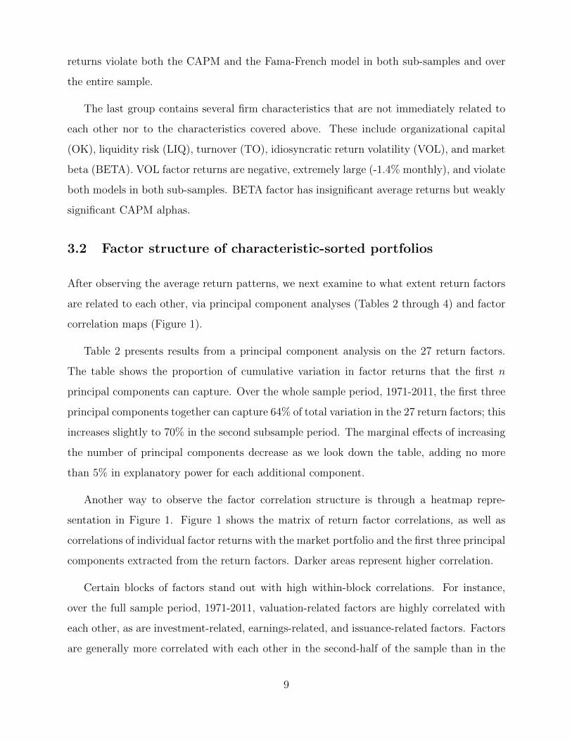
Table 2 presents results from a principal component analysis on the 27 return factors.

The table shows the proportion of cumulative variation in factor returns that the first n

principal components can capture. Over the whole sample period, 1971-2011, the first three

principal components together can capture 64% of total variation in the 27 return factors; this

increases slightly to 70% in the second subsample period. The marginal effects of increasing

the number of principal components decrease as we look down the table, adding no more

than 5% in explanatory power for each additional component.

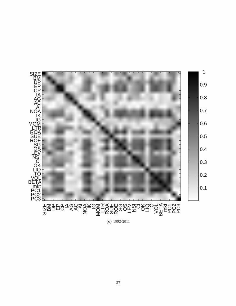
Another way to observe the factor correlation structure is through a heatmap repre-

sentation in Figure 1. Figure 1 shows the matrix of return factor correlations, as well as

correlations of individual factor returns with the market portfolio and the first three principal

components extracted from the return factors. Darker areas represent higher correlation.

Certain blocks of factors stand out with high within-block correlations. For instance,

over the full sample period, 1971-2011, valuation-related factors are highly correlated with

each other, as are investment-related, earnings-related, and issuance-related factors. Factors

are generally more correlated with each other in the second-half of the sample than in the

9

first. This is consistent with better performance of empirical pricing models in the second-

half of the sample, which we discuss below. Some factors stand out as having relatively

low correlation with all other factors. These include accruals (AC), momentum (MOM),

standardized unexpected earnings (SUE), and liquidity risk (LIQ).

Overall, we conclude that there is a substantial degree of comovement among the 27 fac-

tors, indicated both by the high amount of total variance explained by the first three principal

components of the covariance matrix, and by the correlation patterns among economically

related groups of factors.

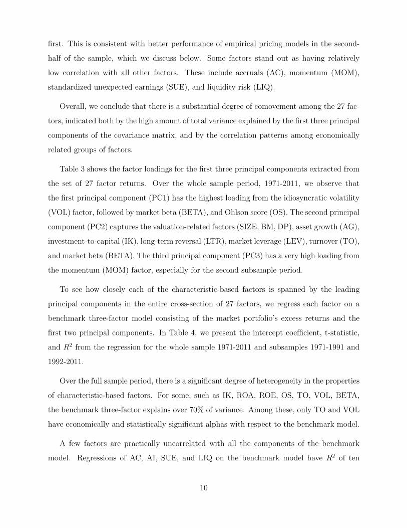
Table 3 shows the factor loadings for the first three principal components extracted from

the set of 27 factor returns. Over the whole sample period, 1971-2011, we observe that

the first principal component (PC1) has the highest loading from the idiosyncratic volatility

(VOL) factor, followed by market beta (BETA), and Ohlson score (OS). The second principal

component (PC2) captures the valuation-related factors (SIZE, BM, DP), asset growth (AG),

investment-to-capital (IK), long-term reversal (LTR), market leverage (LEV), turnover (TO),

and market beta (BETA). The third principal component (PC3) has a very high loading from

the momentum (MOM) factor, especially for the second subsample period.

To see how closely each of the characteristic-based factors is spanned by the leading

principal components in the entire cross-section of 27 factors, we regress each factor on a

benchmark three-factor model consisting of the market portfolio’s excess returns and the

first two principal components. In Table 4, we present the intercept coefficient, t-statistic,

and R2 from the regression for the whole sample 1971-2011 and subsamples 1971-1991 and

1992-2011.

Over the full sample period, there is a significant degree of heterogeneity in the properties

of characteristic-based factors. For some, such as IK, ROA, ROE, OS, TO, VOL, BETA,

the benchmark three-factor explains over 70% of variance. Among these, only TO and VOL

have economically and statistically significant alphas with respect to the benchmark model.

A few factors are practically uncorrelated with all the components of the benchmark

model. Regressions of AC, AI, SUE, and LIQ on the benchmark model have R2 of ten

10

percent or less. All of these except AI have significant alphas with respect to the benchmark

model. The results in Table 4 are largely robust over the two subsamples.

In summary, our analysis of factor correlation suggests that certain groups of characteristic-

based factors can be effectively related to a low-dimensional factor model, but the overall

pattern of results indicates that there is significant remaining heterogeneity among the fac-

tors that a parsimonious model may not be able to capture. In the following section we

further quantify these observations.

3.3 Pricing performance of empirical factor models

In this section, we evaluate the empirical performance of all possible c-factor models con-

structed based on our set of 27 characteristics. As we show in the previous section, the

corresponding 27 c-factors exhibit a non-trivial factor structure. Therefore, several of the

three-factor models may potentially account for the observed average returns differences

within many of the 27 characteristic-sorted portfolio cross-sections. Moreover, since we do

not impose any prior theoretical restrictions on the admissible models, mining through all of

351 possible three-factor models is likely to unearth a few with particularly good in-sample

performance. Thus, while some of the empirical relations between the 27 c-factors are due to

fundamental economic links and therefore the observed performance of such c-factor mod-

els can be grounded in standard theory, it is also clear that the best observed in-sample

performance of c-factor models benefits from a positive bias introduced by data-mining.

Our data-mining exercise is explicit and exhaustive across the space of the 27 charac-

teristics we consider. One can therefore get a sense of the level of performance that can

be achieved by a mechanical search across all candidate models. Evaluating the empirical

c-factor models proposed in the literature is a lot harder because of the lack of information

on how the c-factors and the test portfolios have been chosen among all the possible alter-

natives. This is not necessarily a targeted critique of specific studies; data snooping is a well

known and hard-to-control side-effect of the research process dynamics at the community

level.

11

Table 5 lists twenty best-performing c-factor models, where performance is measured by

the equal-weighted performance measure defined in Section 2. Over the full sample period,

the most successful model uses momentum and cashflow-to-price (CP) factors, and captures

return differences associated with 56% of the considered characteristics (a total of 14 out of

25 test cross-sections). The model ranked in the twentieth place includes return on assets

(ROA) and cashflow-to-price (CP) factors, fitting 44% of the characteristic-sorted cross-

sections. In comparison, the single-factor CAPM and the Fama-French three-factor model,

span 26% (7) and 30% (8) of the characteristics, placing them behind 71% and 48% of all

possible three-factor models in this universe.

The bottom line is that over the 1971-2011 sample period, many randomly constructed

empirical three-factor models comfortably “outperform” both the CAPM and the Fama-

French model, by capturing average return differences among sorted portfolios of as many

as fourteen characteristics on our list.

Over the second half of the sample, three-factor models fit average returns on the

characteristic-sorted portfolios much better than over the full sample, with the best-performing

models matching as many as 84% of the test cross-sections, same as for the first-half of the

sample. The relatively high “success” rate over shorter samples is to be expected, given the

lower statistical power to reject the null of zero model alphas in shorter samples. What is in-

formative is whether the same models tend to exhibit high success rates over the sub-samples;

we investigate such model stability below.

Figure 2 displays the distribution of performance across the c-factor models over the full

sample and the two subsample periods. We use both the equal-weighted method and the

characteristic matching frequency method to measure model performance (see the definitions

in Section 2). For comparison, we indicate the relative performance ranking of the CAPM

and the Fama-French three-factor model relative to all the three-factor models we consider.

Over the full sample (panel (a)), the median-performing three-factor model is able to match

28% of the 25 target portfolio cross-sections, while the median factor model in the first and

second-half sample (panel (c) and (e)) matches 44% and 56% respectively. The Fama-French

model outperforms the CAPM model over the first half of the full sample while substantially

12

underperforming the CAPM over the second half.

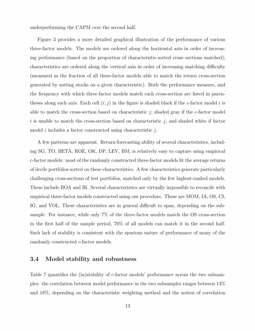
Figure 3 provides a more detailed graphical illustration of the performance of various

three-factor models. The models are ordered along the horizontal axis in order of increas-

ing performance (based on the proportion of characteristic-sorted cross–sections matched);

characteristics are ordered along the vertical axis in order of increasing matching difficulty

(measured as the fraction of all three-factor models able to match the return cross-section

generated by sorting stocks on a given characteristic). Both the performance measure, and

the frequency with which three-factor models match each cross-section are listed in paren-

theses along each axis. Each cell (i, j) in the figure is shaded black if the c-factor model i is

able to match the cross-section based on characteristic j; shaded gray if the c-factor model

i is unable to match the cross-section based on characteristic j, and shaded white if factor

model i includes a factor constructed using characteristic j.

A few patterns are apparent. Return-forecasting ability of several characteristics, includ-

ing SG, TO, BETA, ROE, OK, DP, LEV, BM, is relatively easy to capture using empirical

c-factor models: most of the randomly constructed three-factor models fit the average returns

of decile portfolios sorted on these characteristics. A few characteristics generate particularly

challenging cross-sections of test portfolios, matched only by the few highest-ranked models.

These include ROA and IK. Several characteristics are virtually impossible to reconcile with

empirical three-factor models constructed using our procedure. These are MOM, IA, OS, CI,

IG, and VOL. These characteristics are in general difficult to span, depending on the sub-

sample. For instance, while only 7% of the three-factor models match the OS cross-section

in the first half of the sample period, 70% of all models can match it in the second half.

Such lack of stability is consistent with the spurious nature of performance of many of the

randomly constructed c-factor models.

3.4 Model stability and robustness

Table 7 quantifies the (in)stability of c-factor models’ performance across the two subsam-

ples: the correlation between model performance in the two subsamples ranges between 13%

and 18%, depending on the characteristic weighting method and the notion of correlation

13

statistic. The low degree of correlation in relative model performance across the two sub-

samples is partly due to the sampling errors, but it also suggests that performance of many

models in our set may be spurious.

Another possibility for data-mining is associated with the choice of the empirical proce-

dure for return factor construction. Thus far we have used a straightforward procedure for

constructing return factors as long-short portfolios of the top and bottom deciles of stocks

sorted on each characteristic. One popular alternative approach, following Fama and French

(1993), prescribes a two-dimensional sort: first on firm size and then on a characteristic (in

case of Fama and French (1993), the characteristic is the book-to-market ratio). We apply

a conceptually similar approach in our setting. Specifically, for each characteristic, we first

sort firms into big and small (big firms are above the median in market capitalization, small

firms are below), form 10-1 long-short portfolios within each size class, and then average the

returns on the two long-short portfolios to construct a return factor.

In Table 9, we report cross-sectional correlations of performance between the 351 em-

pirical factor models formed using our univariate factor construction method and the cor-

responding models with factors formed via the double-sorting procedure. While there is no

strong theoretical rationale for using one method of factor construction over the other, the

correlation in empirical model performance across the two methods of forming return factors

is strikingly low, in the range of 22% to 27% over the full sample. In Tables 10 and 11 we

report very different top-twenty and bottom-twenty factor model lists compared to Tables 5

and 6.

We can also compare overall factor model performance using the original one-dimensional

sort factor construction (Figure 3 panel A) and the double-sort factor construction (Figure

4). While we observed in Table 9 a low correlation in model performance across the two

factor construction methods, the relative predictability of characteristics is very similar.

Characteristics that were captured by a large proportion of factor models in Figure 3 are

also captured by a significant number of models in Figure 4. These range from the return on

assets (ROA) characteristic at 37% to the organization capital (OK) characteristic at 60%.

Similarly, investment-to-capital (IK) also appears to be spanned only by the highest-ranked

14

models. Finally, the same list of characteristics remain the most difficult to span: IA, SIZE,

AG, AC, NSI, MOM, VOL, IG, and CI all remain at 5% or less.

We also examine the improvement in model performance caused by moving from a three

to four factor pricing model. We repeat our analysis by considering the universe of 2,925

four-factor models, consisting of the market portfolio and three c-factors based on our list of

27 firm characteristics. We present the results for four-factor models in Appendix B.

The best-performing four-factor model in Table B.1 is able to match 58% of the 24 target

cross-sections, only 2% higher than the best performing three-factor model in Table 5. Many

of the twenty best-performing four-factor models add factors constructed on momentum

(MOM), standardized unexpected earnings (SUE), and asset growth (AG) to one of the

top-performing three-factor models. All of these additions are based on characteristics that

present the most challenge to the three-factor c-models, as we show in Figure 3. Adding such

factors to the three-factor models produces a slight mechanical improvement in performance

by excluding the corresponding cross-section from the set of test portfolios. Beyond that,

the improvement is minimal: most challenging cross-sections have little correlation with each

other or with other c-factors, and therefore it is not possible to capture many additional

cross-sections by introducing a fourth c-factor.

To clarify whether the instability of the factor models is due to the sorted portfolios being

too heavily affected by the smallest firms in our sample, we repeat the key elements of our

analysis of three-factor models on a subsample restricted to 80% of firms with the largest

market capitalization. Overall, we draw very similar conclusions from this subsample as we

do from the full-sample analysis. We summarize the results in Appendix C. As we see in

Table C.2, average returns on the considered empirical factors and their CAPM and Fama-

French alphas are largely similar between the restricted and the full sample of firms. Figure

C.1 shows that the CAPM and the Fama-French three-factor model are close to the median

in their performance relative to all possible three-factor models. Figure C.2 shows significant

similarities to Figure 3: roughly the same set of characteristics is difficult to capture with c-

factor models in the restricted sample as in the full sample, and the characteristics captured

by a large fraction of all possible models are also similar.

15

According to Table C.1, c-factor model performance in a sub-sample excluding the small-

est firms is highly correlated with that in the full sample, although the top 20 and the bottom

20 models are largely different for the restricted sample of largest firms (Tables C.3, C.4).

Model performance is also highly sensitive to the performance measurement convention, as

we show in Table C.5, even more so than over the full sample.

4 Conclusion

The potential hazards of data-mining are well known. Our findings show just how difficult it

is to judge the performance of empirically constructed factor pricing models when both the

return factors and the target cross-sections of assets are chosen in a virtually unrestricted

manner. Starting with a set of 27 commonly used firm characteristics, we show that randomly

constructed characteristic-based factor models can match as many as 56% (14) of the target

return cross-sections over the 1971-2011 sample period.

While the impressive performance of some of the models we consider is spurious, some

models must indeed capture economically meaningful sources of risk. Distinguishing one set

from the other purely based on empirical performance seems difficult. If the factors included

in a theoretically grounded risk-factor model are some of the many possible c-factors, such

a model is likely to be defeated in a pure performance horse-race by the spuriously picked

champions. The winner in such a horse-race is not necessarily a superior risk model. For

example, the momentum factor (MOM) appears in the best-performing three-factor model

for the full sample, and eight (five) of the top twenty portfolios over the first (second) half of

the sample. Yet, without a convincing attribution of the return spread on the momentum-

sorted portfolios to a well-understood source of risk, it is difficult to interpret momentum as

a primitive risk factor of first-order economic importance.

Other situations may be more ambiguous, and one may be able to offer at least a tentative

ex-post theoretical justification for the top-performing model. Such theory-mining can add

a patina of false legitimacy to the spurious pricing models, exacerbating the effects of data-

mining. For example, the top-performing model based on the momentum (MOM) and

16

the cashflow-to-price (CP) factors suggests some tantalizing possibilities for straddling the

behavioral and neoclassical asset pricing paradigms to “motivate” a hybrid pricing model

with empirical performance that is literally second to none. Needless to say, a superficial

theory adds no more value than a spurious empirical result.

In summary, our analysis lends further support to the notion that to distinguish mean-

ingful pricing models from the spurious ones, we should place less weight on the number of

seemingly anomalous return cross-sections the models are able to match, and instead closely

scrutinize the theoretical plausibility and empirical evidence in favor or against their main

economic mechanisms.

17

References

Ang, A., R. Hodrick, Y. Xing, and X. Zhang (2006). The cross-section of volatility and

expected returns. Journal of Finance 61 (1), 259–299.

Baker, M., B. Bradley, and J. Wurgler (2011). Benchmarks as limits to arbitrage: under-

standing the low-volatility anomaly. Financial Analysts Journal 67, 40–54.

Ball, R. and P. Brown (1968). An empirical evaluation of accounting income numbers.

Journal of Accounting Research 6 (2), 159–178.

Banz, R. W. (1981). The relationship between return and market value of common stocks.

Journal of Financial Economics 9, 3–18.

Basu, S. (1977). Investment performance of common stocks in relation to their price-earnings

ratios: a test of the efficient market hypothesis. Journal of Finance 32 (3), 663–682.

Basu, S. (1983). The relationship between earnings’ yield, market value and return for nyse

common stocks. Journal of Financial Economics 12, 129–156.

Bernard, V. L. and J. K. Thomas (1989). Post-earnings-announcement drift: delayed price

response or risk premium? Journal of Accounting Research 27, 1–36.

Bhandari, L. C. (1988). Debt/equity ratio and expected common stock returns: empirical

evidence. Journal of Finance 43 (2), 507–528.

Black, F. (1993). Beta and return. Journal of Political Economy 20, 8–18.

Black, F., M. C. Jensen, and M. S. Scholes (1972). Studies in the Theory of Capital Markets,

Chapter The Capital Asset Pricing Model: Some Empirical Tests. Praeger Publishers Inc.

Chan, L. K. C., Y. Hamao, and J. Lakonishok (1991). Fundamentals and stock returns in

japan. Jouranl of Finance 46 (5), 1739–1764.

Chan, L. K. C., N. Jegadeesh, and J. Lakonishok (1996). Momentum strategies. Journal of

Finance 51 (5), 1681–1713.

18

Chen, L., R. Novy-Marx, and L. Zhang (2010). An alternative three-factor model. working

paper.

Cohen, R. B., P. A. Gompers, and T. Vuolteenaho (2002). Who underreacts to cash-flow

news? evidence from trading between individuals and institutions. Journal of Financial

Economics 66, 409–462.

Cooper, M. J., H. Gulen, and M. J. Schill (2008). Asset growth and the cross-section of

stock returns. Journal of Finance 63 (4), 1609–1651.

Daniel, K. and S. Titman (2006). Market reactions to tangible and intangible information.

Journal of Finance 61 (4), 1605–1643.

DeBondt, W. F. and R. Thaler (1985). Does the stock market overreact? Journal of

Finance 40 (3), 793–805.

Eisfeldt, A. and D. Papanikolaou (2012). Organization capital and the cross-section of

expected returns. Journal of Finance. working paper.

Fairfield, P. M., J. S. Whisenant, and T. L. Yohn (2003). Accrued earnings and growth:

implications for future profitability and market mispricing. The Accounting Review 78

(1), 353–371.

Fama, E. F. and K. French (1993). Common risk factors in the returns on stocks and bonds.

Journal of Financial Economics 33 (1), 3–56.

Fama, E. F. and K. R. French (1992). The cross-section of expected stock returns. Journal

of Finance 47 (2), 427–465.

Fama, E. F. and K. R. French (1996). Multifactor explanations of asset pricing anomalies.

Journal of Finance 51 (1), 55–84.

Fama, E. F. and K. R. French (2006). Profitability, investment and average returns. Journal

of Financial Economics 82, 491–518.

Fama, E. F. and K. R. French (2008). Dissecting anomalies. Journal of Finance 63 (4),

1653–1678.

19

Ferson, W. (1996). Warning: Attribute-sorted portfolios can be hazardous to your research.

In S. Saitou, K. Sawaki, and K. Kubota (Eds.), Modern Finance Theory and its Applica-

tions, pp. 21–32. Center for Academic Societies, Osaka, Japan.

Frazzini, A. and L. Pedersen (2011, October). Betting against beta. working paper.

Gibbons, M. R., S. A. Ross, and J. Shanken (1989). A test of the efficiency of a given

portfolio. Econometrica 57 (5), 1121–1152.

Haugen, R. A. and N. L. Baker (1996). Commonality in the determinants of expected stock

returns. Journal of Financial Economics 41, 401–439.

Hirshleifer, D., K. Hou, S. H. Teoh, and Y. Zhang (2004). Do investors overvalue firms with

bloated balance sheets? Journal of Accounting and Economics 38, 297–331.

Ikenberry, D., J. Lakonishok, and T. Vermaelen (1995). Market underreaction to open market

share repurchases. Journal of Financial Economics 39, 181–208.

Jegadeesh, N. and S. Titman (1993). Returns to buying winners and selling losers: implica-

tions for stock market efficiency. Journal of Finance 48 (1), 65–91.

Lakonishok, J., A. Shleifer, and R. W. Vishny (1994). Contrarian investment, extrapolation,

and risk. Journal of Finance 49 (5), 1541–1578.

Lee, C. M. and B. Swaminathan (2000). Price momentum and trading volume. Journal of

Finance 55 (5), 2017–2069.

Lewellen, J. (2011). The cross-section of expected stock returns. working paper.

Lewellen, J., S. Nagel, and J. Shanken (2010). A skeptical appraisal of asset-pricing tests.

Journal of Financial Economics 96, 175–194.

Litzenberger, R. H. and K. Ramaswamy (1982). The effects of dividends on common stock

prices: tax effects or information effects? Journal of Finance 37 (2), 429–443.

Lo, A. W. and A. C. MacKinlay (1990). Data-snooping biases in tests of financial asset

pricing models. Review of Financial Studies 3 (3), 431–467.

20

Loughran, T. and J. R. Ritter (1995). The new issues puzzle. Journal of Finance 50 (1),

23–51.

Lyandres, E., L. Sun, and L. Zhang (2008). The new issues puzzle: testing the investment-

based explanation. Review of Financial Studies 21 (6), 2825–2855.

Miller, M. H. and M. S. Scholes (1982). Dividends and taxes: some empirical evidence.

Journal of Political Economy 90 (6), 1118–1141.

Novy-Marx, R. (2012, May). Pseudo-predictability in conditional asset pricing tests: ex-

plaining anomaly performance with politics, the weather, global warming, sunspots, and

the stars. working paper.

Ohlson, J. A. (1980). Financial ratios and the probabilistic prediction of bankruptcy. Journal

of Accounting Research 18 (1), 109–131.

Pastor, L. and R. F. Stambaugh (2003). Liquidity risk and expected stock returns. Journal

of Political Economy 111 (3), 642–685.

Piotroski, J. (2000). Value investing: the use of historical financial statement information to

separate winners from losers. Journal of Accounting Research 38, 1–51.

Pontiff, J. and A. Woodgate (2008). Share issuance and cross-sectional returns. Journal of

Finance 63 (2), 921–945.

Rosenberg, B., K. Reid, and R. Lanstein (1985). Persuasive evidence of market inefficiency.

Journal of Portfolio Management 11, 9–17.

Sloan, R. G. (1996). Do stock prices fully reflect information in accruals and cash flows

about future earnings? The Accounting Review 71 (3), 289–315.

Titman, S., K. J. Wei, and F. Xie (2004). Capital investments and stock returns. Journal

of Financial and Quantitative Analysis 39 (4), 677–700.

Xing, Y. (2008). Interpreting the value effect through the q-theory: an empirical investiga-

tion. Review of Financial Studies 21 (4), 1767–1795.

21

Tables and Figures

Table 1 contains the monthly value-weighted average returns, CAPM alphas, and Fama-French alphas for the 27 characteristic-based return factors, over the whole and subsample periods. Factors are the high minus low portfolio from sorting firms into tenportfolios with respect to the underlying firm characteristic. Abbreviations are as follows: size (SIZE), book-to-market (BM),dividend-to-price (DP), earnings-to-price (EP), cash flow-to-price (CP), investment-to-assets (IA), asset growth (AG), accruals(AC), abnormal investment (AI), net operating assets (NOA), investment-to-capital (IK), investment growth (IG), momentum(MOM), long-term reversal (LTR), return on assets (ROA), standardized unexpected earnings (SUE), return on equity (ROE),sales growth (SG), Ohlson score (OS), market leverage (LEV), net stock issues (NSI), composite issuance (CI), organizationcapital (OK), liquidity risk (LIQ), turnover (TO), idiosyncratic volatility (VOL), and market beta (BETA).

Table 1: Characteristics Factors: Summary Statistics

Panel A: Average Returns1971-2011 1971-1991 1992-2011

Characteristic ret t stat ret t stat ret t statSIZE -0.005 -1.81 -0.003 -0.92 -0.006 -1.60BM 0.004 2.18 0.005 1.53 0.004 1.60DP 0.002 0.87 0.001 0.33 0.003 0.91EP 0.007 2.71 0.010 2.95 0.004 1.00CP 0.009 3.49 0.014 4.53 0.004 0.95IA -0.007 -4.37 -0.008 -3.26 -0.007 -2.91AG -0.007 -3.15 -0.006 -2.19 -0.007 -2.27AC -0.006 -2.75 -0.004 -1.40 -0.008 -2.43AI -0.001 -0.84 0.001 0.30 -0.003 -1.40NOA 0.001 0.29 0.003 0.96 -0.002 -0.35IK -0.003 -1.11 -0.005 -1.57 -0.002 -0.35IG -0.004 -2.33 -0.002 -1.12 -0.006 -2.05MOM 0.017 4.41 0.025 6.17 0.009 1.35LTR -0.003 -1.02 -0.002 -0.54 -0.004 -0.88ROA 0.008 2.59 0.007 2.16 0.009 1.69SUE 0.006 2.96 0.007 3.18 0.006 1.59ROE 0.004 1.14 0.006 1.64 0.001 0.27SG -0.002 -1.14 -0.003 -1.04 -0.002 -0.58OS -0.007 -2.01 -0.007 -1.71 -0.007 -1.22LEV 0.004 1.91 0.003 0.97 0.005 1.78NSI -0.005 -3.70 -0.005 -3.07 -0.005 -2.32CI -0.005 -2.57 -0.004 -1.54 -0.006 -2.07OK -0.001 -0.20 -0.001 -0.20 -0.001 -0.11LIQ 0.004 1.78 0.003 1.10 0.004 1.41TO -0.001 -0.36 -0.001 -0.37 -0.001 -0.17VOL -0.014 -3.31 -0.019 -4.69 -0.008 -1.12BETA 0.000 -0.06 0.000 -0.02 0.000 -0.06

22

Panel B: CAPM alpha1971-2011 1971-1991 1992-2011

Characteristic alpha t stat alpha t stat alpha t statSIZE -0.005 -1.56 -0.003 -0.89 -0.006 -1.28BM 0.005 2.48 0.006 1.91 0.004 1.50DP 0.004 2.18 0.003 1.37 0.005 1.69EP 0.009 3.43 0.012 3.19 0.006 1.66CP 0.011 3.98 0.015 4.41 0.006 1.53IA -0.008 -4.19 -0.008 -3.06 -0.007 -2.84AG -0.007 -3.16 -0.007 -2.21 -0.008 -2.28AC -0.006 -3.15 -0.005 -2.24 -0.007 -2.30AI -0.001 -0.67 0.001 0.42 -0.003 -1.52NOA 0.003 1.01 0.005 1.29 0.001 0.27IK -0.006 -2.12 -0.006 -2.68 -0.006 -1.14IG -0.005 -2.38 -0.002 -1.15 -0.007 -2.17MOM 0.018 5.10 0.025 6.42 0.012 1.95LTR -0.003 -0.87 -0.002 -0.56 -0.003 -0.60ROA 0.010 3.25 0.008 2.24 0.013 2.66SUE 0.007 2.23 0.007 2.95 0.008 1.33ROE 0.006 1.73 0.006 1.64 0.006 1.17SG -0.004 -1.97 -0.004 -1.44 -0.004 -1.37OS -0.009 -2.63 -0.009 -1.83 -0.011 -2.00LEV 0.005 1.99 0.004 1.06 0.006 1.66NSI -0.006 -3.61 -0.005 -3.00 -0.007 -2.65CI -0.007 -3.99 -0.005 -2.36 -0.009 -3.29OK -0.003 -0.92 -0.002 -0.60 -0.004 -0.76LIQ 0.004 1.66 0.004 1.34 0.003 0.97TO -0.005 -1.83 -0.004 -1.52 -0.005 -1.22VOL -0.018 -4.58 -0.021 -5.12 -0.015 -2.41BETA -0.006 -1.78 -0.004 -1.08 -0.009 -1.70

23

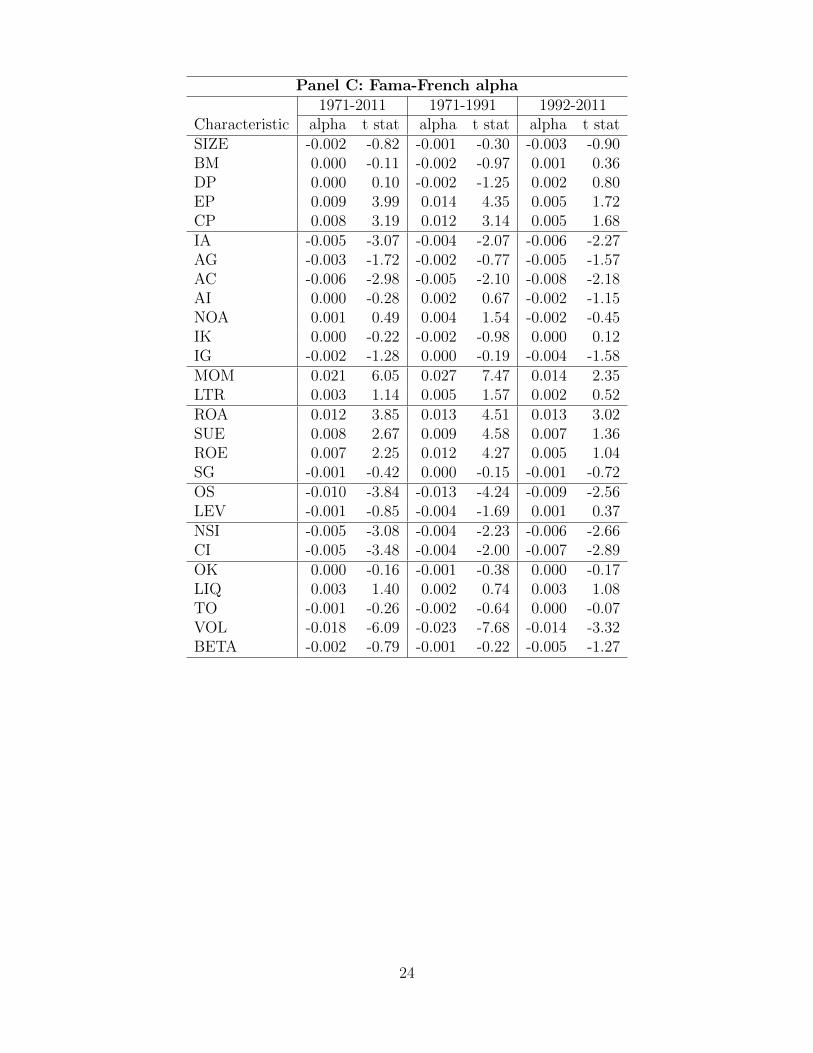
Panel C: Fama-French alpha1971-2011 1971-1991 1992-2011

Characteristic alpha t stat alpha t stat alpha t statSIZE -0.002 -0.82 -0.001 -0.30 -0.003 -0.90BM 0.000 -0.11 -0.002 -0.97 0.001 0.36DP 0.000 0.10 -0.002 -1.25 0.002 0.80EP 0.009 3.99 0.014 4.35 0.005 1.72CP 0.008 3.19 0.012 3.14 0.005 1.68IA -0.005 -3.07 -0.004 -2.07 -0.006 -2.27AG -0.003 -1.72 -0.002 -0.77 -0.005 -1.57AC -0.006 -2.98 -0.005 -2.10 -0.008 -2.18AI 0.000 -0.28 0.002 0.67 -0.002 -1.15NOA 0.001 0.49 0.004 1.54 -0.002 -0.45IK 0.000 -0.22 -0.002 -0.98 0.000 0.12IG -0.002 -1.28 0.000 -0.19 -0.004 -1.58MOM 0.021 6.05 0.027 7.47 0.014 2.35LTR 0.003 1.14 0.005 1.57 0.002 0.52ROA 0.012 3.85 0.013 4.51 0.013 3.02SUE 0.008 2.67 0.009 4.58 0.007 1.36ROE 0.007 2.25 0.012 4.27 0.005 1.04SG -0.001 -0.42 0.000 -0.15 -0.001 -0.72OS -0.010 -3.84 -0.013 -4.24 -0.009 -2.56LEV -0.001 -0.85 -0.004 -1.69 0.001 0.37NSI -0.005 -3.08 -0.004 -2.23 -0.006 -2.66CI -0.005 -3.48 -0.004 -2.00 -0.007 -2.89OK 0.000 -0.16 -0.001 -0.38 0.000 -0.17LIQ 0.003 1.40 0.002 0.74 0.003 1.08TO -0.001 -0.26 -0.002 -0.64 0.000 -0.07VOL -0.018 -6.09 -0.023 -7.68 -0.014 -3.32BETA -0.002 -0.79 -0.001 -0.22 -0.005 -1.27

24

Table 2: Variation Explained: Principal-Component Analysis of Return Factors

PC 1971-2011 1971-1991 1992-20111 0.41 0.31 0.492 0.56 0.52 0.613 0.64 0.60 0.704 0.69 0.66 0.755 0.73 0.71 0.786 0.76 0.75 0.817 0.79 0.78 0.838 0.81 0.81 0.859 0.83 0.83 0.8710 0.85 0.85 0.8811 0.86 0.87 0.9012 0.88 0.88 0.9113 0.89 0.90 0.9214 0.91 0.91 0.9315 0.92 0.92 0.9416 0.93 0.93 0.9517 0.94 0.94 0.9618 0.95 0.95 0.9619 0.96 0.96 0.9720 0.96 0.96 0.9821 0.97 0.97 0.9822 0.98 0.98 0.9923 0.98 0.98 0.9924 0.99 0.99 0.9925 0.99 0.99 1.0026 1.00 1.00 1.0027 1 1 1

Table 2 presents results from a principal component analysis on the 27 characteristic-based return factors. Factors are the highminus low portfolio from sorting firms into ten portfolios with respect to the underlying firm characteristic. The table showsthe proportion of cumulative variation that the first n principal components can capture. Results are presented over the wholesample period 1971-2011 and subsamples 1971-1991 and 1992-2011.

25

Table 3: Principal-Component Factor Loadings

1971-2011 1971-1991 1992-2011PC1 PC2 PC3 PC1 PC2 PC3 PC1 PC2 PC3

SIZE -0.17 0.25 -0.12 -0.30 0.05 0.10 -0.13 0.28 -0.12BM -0.03 -0.25 0.01 0.15 -0.28 0.33 -0.04 -0.16 0.00DP -0.12 -0.24 -0.01 0.01 -0.34 0.14 -0.11 -0.19 0.02EP -0.21 0.09 0.05 -0.24 -0.08 0.23 -0.19 0.13 0.02CP -0.18 -0.03 0.03 -0.02 -0.16 0.45 -0.20 0.12 -0.06IA 0.00 0.17 -0.11 -0.09 0.15 0.00 0.01 0.15 -0.12AG -0.01 0.28 -0.10 -0.17 0.18 0.04 0.02 0.29 -0.11AC 0.01 0.06 -0.04 0.08 0.15 0.11 -0.03 0.06 0.00AI -0.04 0.06 -0.13 -0.08 -0.01 -0.04 -0.03 0.07 -0.14NOA -0.23 -0.04 -0.18 -0.24 -0.17 -0.03 -0.20 -0.11 -0.17IK 0.23 0.27 -0.06 0.02 0.29 -0.11 0.25 0.27 -0.06IG 0.03 0.14 -0.10 -0.04 0.08 -0.02 0.05 0.19 -0.12MOM -0.12 0.20 0.90 -0.17 0.08 0.33 -0.11 0.30 0.86LTR -0.14 0.39 -0.12 -0.30 0.20 0.04 -0.11 0.44 -0.23ROA -0.29 0.18 0.02 -0.29 0.07 0.10 -0.30 0.15 0.00SUE -0.07 0.07 0.13 -0.09 0.05 0.05 -0.06 0.05 0.12ROE -0.27 0.19 -0.09 -0.31 0.08 -0.01 -0.28 0.14 -0.07SG 0.13 0.16 -0.02 -0.02 0.21 0.00 0.14 0.11 0.02OS 0.34 -0.18 0.16 0.43 0.04 -0.04 0.31 -0.15 0.17LEV -0.03 -0.30 -0.03 0.19 -0.24 0.31 -0.06 -0.25 -0.03NSI 0.08 0.06 0.00 -0.01 0.06 -0.11 0.09 0.04 0.02CI 0.13 0.09 -0.06 0.08 0.18 -0.17 0.13 0.06 -0.06OK 0.25 0.08 0.12 0.19 0.18 -0.10 0.25 0.10 0.15LIQ 0.02 0.00 -0.03 0.01 -0.11 -0.23 0.04 0.11 -0.05TO 0.24 0.25 0.05 0.10 0.35 0.25 0.25 0.25 0.02VOL 0.41 -0.10 -0.03 0.36 0.14 0.17 0.41 -0.15 -0.05BETA 0.36 0.31 -0.08 0.11 0.44 0.40 0.39 0.25 -0.13

Table 3 presents factor loadings for the first three principal components extracted from the set of 27 factor returns. Loadingsare shown for the whole sample period 1971-2011 and subsamples 1971-1991 and 1992-2011.

Characteristic abbreviations are as follows: size (SIZE), book-to-market (BM), dividend-to-price (DP), earnings-to-price (EP),cash flow-to-price (CP), investment-to-assets (IA), asset growth (AG), accruals (AC), abnormal investment (AI), net operatingassets (NOA), investment-to-capital (IK), investment growth (IG), momentum (MOM), long-term reversal (LTR), return onassets (ROA), standardized unexpected earnings (SUE), return on equity (ROE), sales growth (SG), Ohlson score (OS), marketleverage (LEV), net stock issues (NSI), composite issuance (CI), organization capital (OK), liquidity risk (LIQ), turnover (TO),idiosyncratic return volatility (VOL), and market beta (BETA). Details on characteristic definitions and construction is inAppendix A.

26

Table 4: Factor Regression on the Principal-Component Model

1971-2011 1971-1991 1992-2011factor alpha t stat R2 alpha t stat R2 alpha t stat R2

SIZE -0.009 -4.56 0.59 -0.012 -4.40 0.68 -0.009 -3.00 0.57BM 0.002 1.39 0.49 0.002 0.99 0.63 0.001 0.66 0.37DP 0.000 -0.03 0.54 -0.003 -1.19 0.63 0.001 0.38 0.50EP 0.004 1.92 0.56 0.006 1.88 0.47 0.001 0.63 0.64CP 0.004 1.85 0.40 0.010 2.88 0.15 0.001 0.20 0.65IA -0.007 -4.35 0.31 -0.007 -3.36 0.37 -0.006 -2.75 0.24AG -0.005 -3.24 0.51 -0.006 -3.11 0.55 -0.006 -2.29 0.45AC -0.007 -2.78 0.03 -0.002 -0.70 0.25 -0.008 -2.13 0.04AI -0.002 -1.23 0.09 -0.001 -0.23 0.11 -0.004 -2.06 0.09NOA -0.005 -2.20 0.57 -0.005 -1.96 0.67 -0.006 -2.16 0.59IK 0.003 1.77 0.77 0.000 -0.11 0.57 0.004 1.71 0.85IG -0.002 -1.51 0.23 -0.001 -0.32 0.14 -0.005 -1.98 0.30MOM 0.017 3.82 0.16 0.023 5.76 0.16 0.012 1.85 0.21LTR -0.004 -2.17 0.69 -0.004 -1.73 0.68 -0.003 -1.23 0.69ROA 0.003 1.61 0.75 0.004 1.66 0.63 0.005 2.20 0.81SUE 0.006 2.07 0.10 0.006 2.73 0.19 0.007 1.24 0.08ROE -0.001 -0.68 0.74 0.002 0.78 0.72 -0.002 -0.52 0.76SG 0.001 0.75 0.50 0.000 -0.07 0.34 0.002 0.89 0.65OS 0.000 0.15 0.81 0.003 1.39 0.83 -0.001 -0.46 0.80LEV 0.001 0.53 0.60 0.001 0.39 0.62 0.001 0.75 0.57NSI -0.003 -2.17 0.29 -0.004 -2.11 0.08 -0.004 -1.78 0.44CI -0.003 -1.84 0.44 0.000 -0.04 0.39 -0.005 -2.16 0.51OK 0.006 3.04 0.66 0.007 2.64 0.57 0.005 1.76 0.71LIQ 0.005 2.05 0.01 0.003 0.85 0.08 0.004 1.39 0.12TO 0.003 2.14 0.79 0.003 1.39 0.67 0.003 1.84 0.87VOL -0.006 -2.98 0.82 -0.011 -4.09 0.73 -0.004 -1.20 0.85BETA 0.004 1.75 0.78 0.005 1.60 0.64 0.001 0.33 0.85

Table 4 presents results from regressing the characteristic-based return factors on the benchmark three-factor model, consistingof the market portfolio and the first two principal component vectors of the return factors. Factors are the high minus low port-folio from sorting firms into ten portfolios with respect to the underlying firm characteristic. The alpha coefficient, t-statistic,and R2 from the regression is shown in the table for the whole sample period 1971-2011 and subsamples 1971-1991 and 1992-2011.


27

Table 5: Top 20 Performing Factor Models

1971-2011 1971-1991 1992-2011C1 C2 prop C1 C2 prop C1 C2 prop

1 MOM CP 0.56 MOM IA 0.84 AG SUE 0.842 SUE CP 0.56 MOM CP 0.84 AG EP 0.843 SIZE VOL 0.52 MOM IK 0.80 AG CP 0.844 AG CP 0.52 MOM LTR 0.72 SUE CI 0.805 AI CP 0.52 MOM AG 0.72 SIZE VOL 0.766 CP IG 0.52 IA SUE 0.72 BM SUE 0.767 BM SUE 0.48 IA EP 0.72 MOM NSI 0.768 EP CP 0.48 OS AG 0.72 ROA AG 0.769 EP IG 0.48 BM MOM 0.68 AG VOL 0.7610 EP LIQ 0.48 MOM LEV 0.68 SUE LEV 0.7611 AC CP 0.48 MOM LIQ 0.68 SUE AC 0.7612 ROE CP 0.48 IA OS 0.68 CI LIQ 0.7613 NOA CP 0.48 AC CP 0.68 CP IG 0.7614 CP LIQ 0.48 AI CP 0.68 BM MOM 0.7215 BM MOM 0.44 NOA CP 0.68 MOM SUE 0.7216 BM CP 0.44 NOA IK 0.68 MOM LEV 0.7217 MOM OS 0.44 CP IG 0.68 MOM CI 0.7218 MOM EP 0.44 CP LIQ 0.68 LTR VOL 0.7219 MOM VOL 0.44 IA ROA 0.64 OS IG 0.7220 ROA CP 0.44 ROA CP 0.64 NSI SUE 0.72

Table 5 lists the characteristic-based factors that constitute the top twenty linear factor models, in terms of the proportion ofremaining characteristics they can capture, via the equal-weighted method. We say that a factor model M captures, or spans,a characteristic C, if the p-value from the Gibbons et al. (1989) F-test of joint significance of abnormal average return withrespect to M across the ten sorted portfolios on C is above 10%. Top factor models are shown for the whole sample period1971-2011 and subsamples 1971-1991 and 1992-2011.

The universe of factor models is all three-factor models consisting of the market portfolio and two characteristic return factors(C1, C2) from our list of 27. Characteristic abbreviations are as follows: size (SIZE), book-to-market (BM), dividend-to-price(DP), earnings-to-price (EP), cash flow-to-price (CP), investment-to-assets (IA), asset growth (AG), accruals (AC), abnormalinvestment (AI), net operating assets (NOA), investment-to-capital (IK), investment growth (IG), momentum (MOM), long-term reversal (LTR), return on assets (ROA), standardized unexpected earnings (SUE), return on equity (ROE), sales growth(SG), Ohlson score (OS), market leverage(LEV), net stock issues (NSI), composite issuance (CI), organization capital (OK),liquidity risk (LIQ), turnover (TO), idiosyncratic return volatility (VOL), and market beta (BETA). Details on characteristicdefinitions and construction is in Appendix A.

28

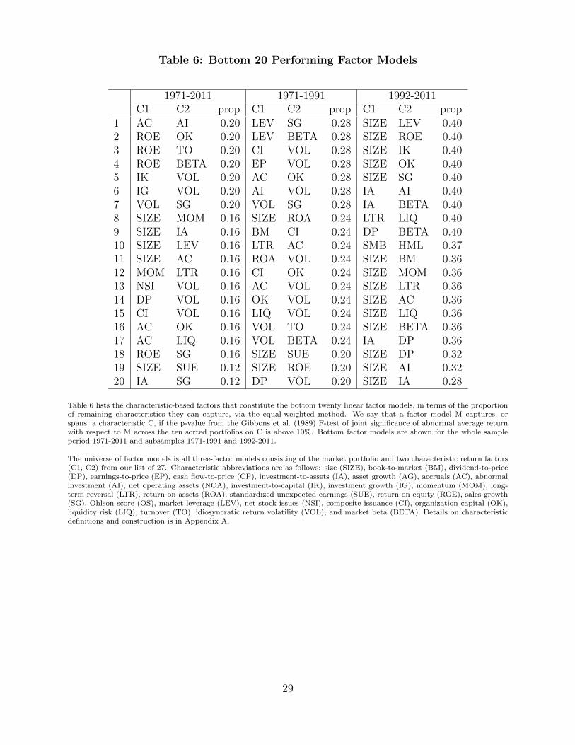
Table 6: Bottom 20 Performing Factor Models


1 AC AI 0.20 LEV SG 0.28 SIZE LEV 0.402 ROE OK 0.20 LEV BETA 0.28 SIZE ROE 0.403 ROE TO 0.20 CI VOL 0.28 SIZE IK 0.404 ROE BETA 0.20 EP VOL 0.28 SIZE OK 0.405 IK VOL 0.20 AC OK 0.28 SIZE SG 0.406 IG VOL 0.20 AI VOL 0.28 IA AI 0.407 VOL SG 0.20 VOL SG 0.28 IA BETA 0.408 SIZE MOM 0.16 SIZE ROA 0.24 LTR LIQ 0.409 SIZE IA 0.16 BM CI 0.24 DP BETA 0.4010 SIZE LEV 0.16 LTR AC 0.24 SMB HML 0.3711 SIZE AC 0.16 ROA VOL 0.24 SIZE BM 0.3612 MOM LTR 0.16 CI OK 0.24 SIZE MOM 0.3613 NSI VOL 0.16 AC VOL 0.24 SIZE LTR 0.3614 DP VOL 0.16 OK VOL 0.24 SIZE AC 0.3615 CI VOL 0.16 LIQ VOL 0.24 SIZE LIQ 0.3616 AC OK 0.16 VOL TO 0.24 SIZE BETA 0.3617 AC LIQ 0.16 VOL BETA 0.24 IA DP 0.3618 ROE SG 0.16 SIZE SUE 0.20 SIZE DP 0.3219 SIZE SUE 0.12 SIZE ROE 0.20 SIZE AI 0.3220 IA SG 0.12 DP VOL 0.20 SIZE IA 0.28

Table 6 lists the characteristic-based factors that constitute the bottom twenty linear factor models, in terms of the proportionof remaining characteristics they can capture, via the equal-weighted method. We say that a factor model M captures, orspans, a characteristic C, if the p-value from the Gibbons et al. (1989) F-test of joint significance of abnormal average returnwith respect to M across the ten sorted portfolios on C is above 10%. Bottom factor models are shown for the whole sampleperiod 1971-2011 and subsamples 1971-1991 and 1992-2011.

The universe of factor models is all three-factor models consisting of the market portfolio and two characteristic return factors(C1, C2) from our list of 27. Characteristic abbreviations are as follows: size (SIZE), book-to-market (BM), dividend-to-price(DP), earnings-to-price (EP), cash flow-to-price (CP), investment-to-assets (IA), asset growth (AG), accruals (AC), abnormalinvestment (AI), net operating assets (NOA), investment-to-capital (IK), investment growth (IG), momentum (MOM), long-term reversal (LTR), return on assets (ROA), standardized unexpected earnings (SUE), return on equity (ROE), sales growth(SG), Ohlson score (OS), market leverage (LEV), net stock issues (NSI), composite issuance (CI), organization capital (OK),liquidity risk (LIQ), turnover (TO), idiosyncratic return volatility (VOL), and market beta (BETA). Details on characteristicdefinitions and construction is in Appendix A.

29

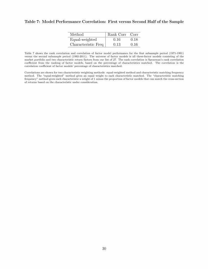
Table 7: Model Performance Correlation: First versus Second Half of the Sample

Method Rank Corr CorrEqual-weighted 0.16 0.18Characteristic Freq 0.13 0.16

Table 7 shows the rank correlation and correlation of factor model performance for the first subsample period (1971-1991)versus the second subsample period (1992-2011). The universe of factor models is all three-factor models consisting of themarket portfolio and two characteristic return factors from our list of 27. The rank correlation is Spearman’s rank correlationcoefficient from the ranking of factor models, based on the percentage of characteristics matched. The correlation is thecorrelation coefficient of factor models’ percentage of characteristics matched.

Correlations are shown for two characteristic weighting methods: equal-weighted method and characteristic matching frequencymethod. The “equal-weighted” method gives an equal weight to each characteristic matched. The “characteristic matchingfrequency” method gives each characteristic a weight of 1 minus the proportion of factor models that can match the cross-sectionof returns based on the characteristic under consideration.

30

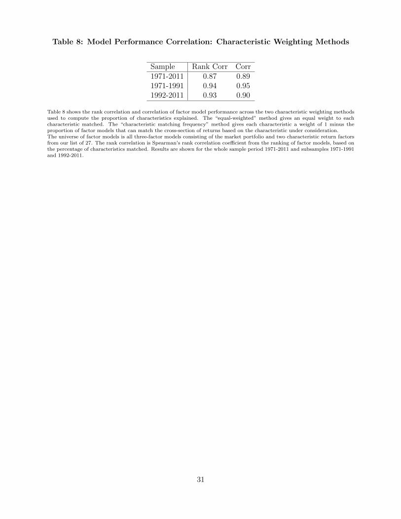
Table 8: Model Performance Correlation: Characteristic Weighting Methods

Sample Rank Corr Corr1971-2011 0.87 0.891971-1991 0.94 0.951992-2011 0.93 0.90

Table 8 shows the rank correlation and correlation of factor model performance across the two characteristic weighting methodsused to compute the proportion of characteristics explained. The “equal-weighted” method gives an equal weight to eachcharacteristic matched. The “characteristic matching frequency” method gives each characteristic a weight of 1 minus theproportion of factor models that can match the cross-section of returns based on the characteristic under consideration.The universe of factor models is all three-factor models consisting of the market portfolio and two characteristic return factorsfrom our list of 27. The rank correlation is Spearman’s rank correlation coefficient from the ranking of factor models, based onthe percentage of characteristics matched. Results are shown for the whole sample period 1971-2011 and subsamples 1971-1991and 1992-2011.

31

Table 9: Model Performance Correlation: Factor Construction

1971-2011 1971-1991 1992-2011Method rank corr corr rank corr corr rank corr corrEqual-weighted 0.26 0.27 0.42 0.43 0.35 0.38Characteristic Freq 0.22 0.24 0.41 0.44 0.24 0.17

Table 9 shows the rank correlation and correlation of factor model performance across the two different methods to constructcharacteristic-based return factors. The default method is to construct the factor as the high minus low portfolio of a one-waysort. The second method is to construct the factor as the equal-weighed average of the high minus low portfolio within the bigand small size group, from a double-sort first on size and then the characteristic.

The universe of factor models is all three-factor models consisting of the market portfolio and two characteristic return factorsfrom our list of 27. The rank correlation is Spearman’s rank correlation coefficient from the ranking of factor models, basedon the percentage of characteristics matched. The correlation is the correlation coefficient of factor models’ percentage ofcharacteristics matched.

Correlations are shown for two characteristic weighting methods, equal-weighted method and characteristic matching frequencymethod, as well as for the whole sample period 1971-2011 and subsamples 1971-1991 and 1992-2011. The “equal-weighted”method gives an equal weight to each characteristic matched. The “characteristic matching frequency” method gives eachcharacteristic a weight of 1 minus the proportion of factor models that can match the cross-section of returns based on thecharacteristic under consideration.

32

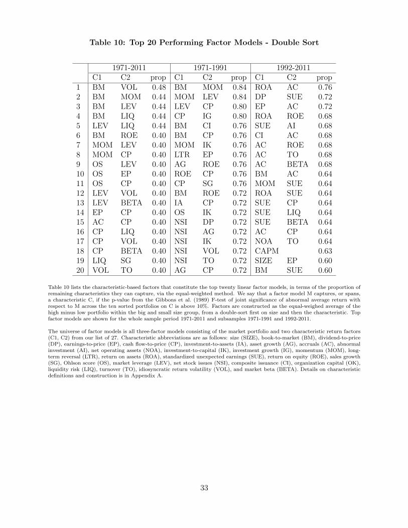
Table 10: Top 20 Performing Factor Models - Double Sort


1 BM VOL 0.48 BM MOM 0.84 ROA AC 0.762 BM MOM 0.44 MOM LEV 0.84 DP SUE 0.723 BM LEV 0.44 LEV CP 0.80 EP AC 0.724 BM LIQ 0.44 CP IG 0.80 ROA ROE 0.685 LEV LIQ 0.44 BM CI 0.76 SUE AI 0.686 BM ROE 0.40 BM CP 0.76 CI AC 0.687 MOM LEV 0.40 MOM IK 0.76 AC ROE 0.688 MOM CP 0.40 LTR EP 0.76 AC TO 0.689 OS LEV 0.40 AG ROE 0.76 AC BETA 0.6810 OS EP 0.40 ROE CP 0.76 BM AC 0.6411 OS CP 0.40 CP SG 0.76 MOM SUE 0.6412 LEV VOL 0.40 BM ROE 0.72 ROA SUE 0.6413 LEV BETA 0.40 IA CP 0.72 SUE CP 0.6414 EP CP 0.40 OS IK 0.72 SUE LIQ 0.6415 AC CP 0.40 NSI DP 0.72 SUE BETA 0.6416 CP LIQ 0.40 NSI AG 0.72 AC CP 0.6417 CP VOL 0.40 NSI IK 0.72 NOA TO 0.6418 CP BETA 0.40 NSI VOL 0.72 CAPM 0.6319 LIQ SG 0.40 NSI TO 0.72 SIZE EP 0.6020 VOL TO 0.40 AG CP 0.72 BM SUE 0.60

Table 10 lists the characteristic-based factors that constitute the top twenty linear factor models, in terms of the proportion ofremaining characteristics they can capture, via the equal-weighted method. We say that a factor model M captures, or spans,a characteristic C, if the p-value from the Gibbons et al. (1989) F-test of joint significance of abnormal average return withrespect to M across the ten sorted portfolios on C is above 10%. Factors are constructed as the equal-weighed average of thehigh minus low portfolio within the big and small size group, from a double-sort first on size and then the characteristic. Topfactor models are shown for the whole sample period 1971-2011 and subsamples 1971-1991 and 1992-2011.


33

Table 11: Bottom 20 Performing Factor Models - Double Sort


1 CI IG 0.08 OS SUE 0.20 LTR NSI 0.202 AC AI 0.08 SUE AC 0.20 LTR CI 0.203 AC LIQ 0.08 SUE IG 0.20 LTR BETA 0.204 SIZE MOM 0.04 SUE LIQ 0.20 NSI NOA 0.205 SIZE SUE 0.04 SUE TO 0.20 AG CI 0.206 BM IA 0.04 NOA OK 0.20 AG AC 0.207 MOM NSI 0.04 SIZE LTR 0.16 AG LIQ 0.208 IA ROA 0.04 SIZE ROE 0.16 SIZE LTR 0.169 IA DP 0.04 ROA SUE 0.16 SIZE DP 0.1610 IA SUE 0.04 ROA AC 0.16 SIZE AG 0.1611 IA CI 0.04 SUE EP 0.16 SIZE AC 0.1612 IA ROE 0.04 SUE ROE 0.16 SIZE AI 0.1613 IA VOL 0.04 SUE OK 0.16 SIZE LIQ 0.1614 ROA IK 0.04 SUE VOL 0.16 MOM IA 0.1615 NSI SUE 0.04 SUE BETA 0.16 IA NSI 0.1616 NSI LEV 0.04 SIZE ROA 0.12 IA AG 0.1617 NSI AI 0.04 DP SUE 0.12 IA AC 0.1618 NSI TO 0.04 SUE CI 0.12 SIZE MOM 0.1219 AG CI 0.04 SUE NOA 0.12 SIZE IA 0.1220 ROA NSI 0.00 SIZE SUE 0.04 IA CI 0.12

Table 11 lists the characteristic-based factors that constitute the bottom twenty linear factor models, in terms of the proportionof remaining characteristics they can capture, via the equal-weighted method. We say that a factor model M captures,or spans, a characteristic C, if the p-value from the Gibbons et al. (1989) F-test of joint significance of abnormal averagereturn with respect to M across the ten sorted portfolios on C is above 10%. Factors are constructed as the equal-weighedaverage of the high minus low portfolio within the big and small size group, from a double-sort first on size and then thecharacteristic. Bottom factor models are shown for the whole sample period 1971-2011 and subsamples 1971-1991 and 1992-2011.


34

Figure 1: Factor Correlation

Figure 1 shows a heatmap representation of the correlation matrix for the 27 characteristic-based factors, the market portfolio,and the first three principal components extracted from the return factors. The magnitude of correlations is represented in thefigure, with darker areas representing higher correlation.

Factors are the high minus low portfolio from sorting firms into ten portfolios with respect to the underlying firm characteristic.Characteristic abbreviations are as follows: size (SIZE), book-to-market (BM), dividend-to-price (DP), earnings-to-price (EP),cash flow-to-price (CP), investment-to-assets (IA), asset growth (AG), accruals (AC), abnormal investment (AI), net operatingassets (NOA), investment-to-capital (IK), investment growth (IG), momentum (MOM), long-term reversal (LTR), return onassets (ROA), standardized unexpected earnings (SUE), return on equity (ROE), sales growth (SG), Ohlson score (OS), marketleverage(LEV), net stock issues (NSI), composite issuance (CI), organization capital (OK), liquidity risk (LIQ), turnover (TO),idiosyncratic return volatility (VOL), and market beta (BETA). Details on characteristic definitions and construction is inAppendix A.

(a) 1971-2011

SIZ

EB

M DP

EP

CP IA AG

AC AI

NO

A IK IGM

OM

LTR

RO

AS

UE

RO

ES

GO

SLE

VN

SI

CI

OK

LIQ TO

VO

LB

ET

Am

ktP

C1

PC

2P

C3

SIZEBMDPEPCPIA

AGACAI

NOAIKIG

MOMLTR

ROASUEROE

SGOS

LEVNSI

CIOKLIQTO

VOLBETA

mktPC1PC2PC3

0.1

0.2

0.3

0.4

0.5

0.6

0.7

0.8

0.9

1

35

SIZ

EB

M DP

EP

CP IA AG

AC AI

NO

A IK IGM

OM

LTR

RO

AS

UE

RO

ES

GO

SLE

VN

SI

CI

OK

LIQ TO

VO

LB

ET

Am

ktP

C1

PC

2P

C3

SIZEBMDPEPCPIA

AGACAI

NOAIKIG

MOMLTR

ROASUEROE

SGOS

LEVNSI

CIOKLIQTO

VOLBETA

mktPC1PC2PC3

0.1

0.2

0.3

0.4

0.5

0.6

0.7

0.8

0.9

1

(b) 1971-1991

36

SIZ

EB

M DP

EP

CP IA AG

AC AI

NO

A IK IGM

OM

LTR

RO

AS

UE

RO

ES

GO

SLE

VN

SI

CI

OK

LIQ TO

VO

LB

ET

Am

ktP

C1

PC

2P

C3

SIZEBMDPEPCPIA

AGACAI

NOAIKIG

MOMLTR

ROASUEROE

SGOS

LEVNSI

CIOKLIQTO

VOLBETA

mktPC1PC2PC3

0.1

0.2

0.3

0.4

0.5

0.6

0.7

0.8

0.9

1

(c) 1992-2011

37

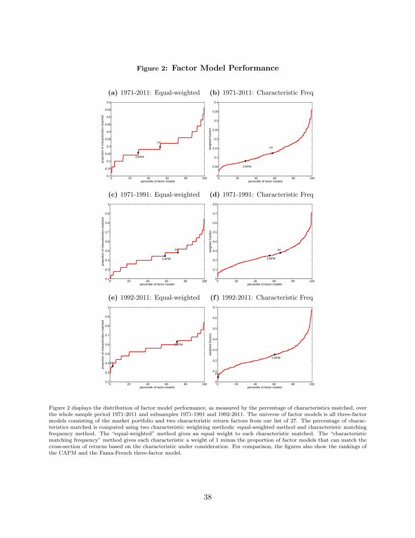
Figure 2: Factor Model Performance

(a) 1971-2011: Equal-weighted

0 20 40 60 80 1000.1

0.15

0.2

0.25

0.3

0.35

0.4

0.45

0.5

0.55

0.6

CAPM

FF

percentile of factor models

prop

ortio

n of

cha

ract

eris

tics

mat

ched

(b) 1971-2011: Characteristic Freq

0 20 40 60 80 1000

0.05

0.1

0.15

0.2

0.25

0.3

0.35

0.4

CAPM

FF


wei

ghte

d fr

actio

n

(c) 1971-1991: Equal-weighted

0 20 40 60 80 1000.2

0.3

0.4

0.5

0.6

0.7

0.8

0.9

1

CAPM

FF


prop

ortio

n of

cha

ract

eris

tics

mat

ched

(d) 1971-1991: Characteristic Freq

0 20 40 60 80 1000

0.1

0.2

0.3

0.4

0.5

0.6

0.7

0.8

CAPM

FF


wei

ghte

d fr

actio

n

(e) 1992-2011: Equal-weighted

0 20 40 60 80 1000.2

0.3

0.4

0.5

0.6

0.7

0.8

0.9

1

CAPM

FF


prop

ortio

n of

cha

ract

eris

tics

mat

ched

(f) 1992-2011: Characteristic Freq

0 20 40 60 80 1000

0.1

0.2

0.3

0.4

0.5

0.6

0.7

CAPM

FF


wei

ghte

d fr

actio

n

Figure 2 displays the distribution of factor model performance, as measured by the percentage of characteristics matched, overthe whole sample period 1971-2011 and subsamples 1971-1991 and 1992-2011. The universe of factor models is all three-factormodels consisting of the market portfolio and two characteristic return factors from our list of 27. The percentage of charac-teristics matched is computed using two characteristic weighting methods: equal-weighted method and characteristic matchingfrequency method. The “equal-weighted” method gives an equal weight to each characteristic matched. The “characteristicmatching frequency” method gives each characteristic a weight of 1 minus the proportion of factor models that can match thecross-section of returns based on the characteristic under consideration. For comparison, the figures also show the rankings ofthe CAPM and the Fama-French three-factor model.

38

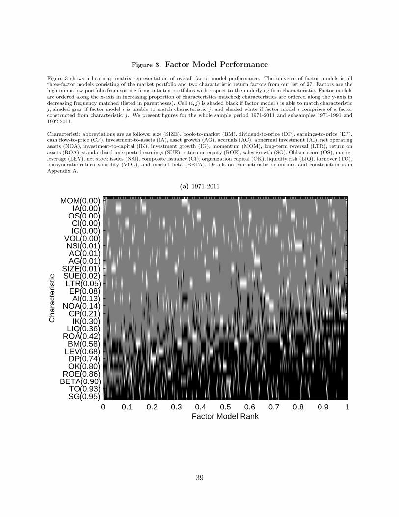
Figure 3: Factor Model Performance

Figure 3 shows a heatmap matrix representation of overall factor model performance. The universe of factor models is allthree-factor models consisting of the market portfolio and two characteristic return factors from our list of 27. Factors are thehigh minus low portfolio from sorting firms into ten portfolios with respect to the underlying firm characteristic. Factor modelsare ordered along the x-axis in increasing proportion of characteristics matched; characteristics are ordered along the y-axis indecreasing frequency matched (listed in parentheses). Cell (i, j) is shaded black if factor model i is able to match characteristicj, shaded gray if factor model i is unable to match characteristic j, and shaded white if factor model i comprises of a factorconstructed from characteristic j. We present figures for the whole sample period 1971-2011 and subsamples 1971-1991 and1992-2011.


(a) 1971-2011

Cha

ract

eris

tic

Factor Model Rank0 0.1 0.2 0.3 0.4 0.5 0.6 0.7 0.8 0.9 1

MOM(0.00)IA(0.00)

OS(0.00)CI(0.00)IG(0.00)

VOL(0.00)NSI(0.01)AC(0.01)AG(0.01)

SIZE(0.01)SUE(0.02)LTR(0.05)EP(0.08)AI(0.13)

NOA(0.14)CP(0.21)IK(0.30)

LIQ(0.36)ROA(0.42)

BM(0.58)LEV(0.68)DP(0.74)OK(0.80)

ROE(0.86)BETA(0.90)

TO(0.93)SG(0.95)

39

Cha

ract

eris

tic


SIZE(0.00)MOM(0.00)VOL(0.00)

CP(0.05)OS(0.07)EP(0.09)

NOA(0.15)IK(0.21)IA(0.25)

AG(0.25)AI(0.28)

NSI(0.29)SUE(0.34)

CI(0.41)ROE(0.47)

IG(0.48)LEV(0.55)BM(0.56)

ROA(0.63)AC(0.64)DP(0.77)

LTR(0.86)BETA(0.86)

OK(0.91)SG(0.92)TO(0.98)LIQ(1.00)

(b) 1971-1991

40

Cha

ract

eris

tic


LTR(0.00)SUE(0.00)

AG(0.00)IG(0.02)CI(0.05)

NSI(0.08)TO(0.11)EP(0.14)

VOL(0.42)AC(0.50)IA(0.51)

ROA(0.53)AI(0.55)

SIZE(0.62)OS(0.70)CP(0.78)

NOA(0.80)OK(0.81)

MOM(0.90)ROE(0.91)

SG(0.93)IK(0.98)

BETA(0.99)LIQ(1.00)BM(1.00)DP(1.00)

LEV(1.00)

(c) 1992-2011

41

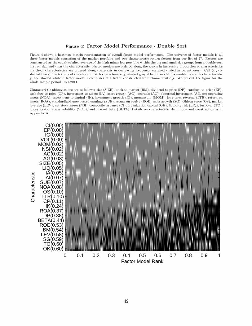
Figure 4: Factor Model Performance - Double Sort

Figure 4 shows a heatmap matrix representation of overall factor model performance. The universe of factor models is allthree-factor models consisting of the market portfolio and two characteristic return factors from our list of 27. Factors areconstructed as the equal-weighed average of the high minus low portfolio within the big and small size group, from a double-sortfirst on size and then the characteristic. Factor models are ordered along the x-axis in increasing proportion of characteristicsmatched; characteristics are ordered along the y-axis in decreasing frequency matched (listed in parentheses). Cell (i, j) isshaded black if factor model i is able to match characteristic j, shaded gray if factor model i is unable to match characteristicj, and shaded white if factor model i comprises of a factor constructed from characteristic j. We present the figure for thewhole sample period 1971-2011.


Cha

ract

eris

tic


CI(0.00)EP(0.00)IG(0.00)

VOL(0.00)MOM(0.02)

NSI(0.02)AC(0.02)AG(0.03)

SIZE(0.05)LIQ(0.05)

IA(0.05)AI(0.07)

SUE(0.07)NOA(0.08)

OS(0.10)LTR(0.10)CP(0.11)IK(0.24)

ROA(0.37)DP(0.38)

BETA(0.44)ROE(0.53)

BM(0.54)LEV(0.58)SG(0.59)TO(0.60)OK(0.60)

42

A Appendix: Construction of Characteristics

We provide details on the definitions and construction of 27 firm characteristics.

A.1 Valuation

Size (SIZE)

Stocks with low market capitalization have abnormally high average returns (Banz (1981), Fama and French (1992)). Size isdefined to be the log of market capitalization.

Book-to-Market (BM)

Stocks with high book-to-market have abnormally high average returns (Rosenberg, Reid, and Lanstein (1985), Chan, Hamao,and Lakonishok (1991), Fama and French (1992)). The effect remains after controlling for many other variables and is strongestamong smaller stocks (Fama and French (1993), Fama and French (2008)).

Dividend-to-Price (DP)

There is a positive association between stock returns and dividend yield (Litzenberger and Ramaswamy (1982), Miller andScholes (1982)). However, more recently, it has been shown that dividend yield has little predictive power for future returns(Lewellen (2011)).

Earnings-to-Price (EP)

Stocks with high earnings-to-price have abnormally high average returns (Basu (1977), Basu (1983)). The effect seems to besubsumed by size and book-to-market (Fama and French (1992), Fama and French (1996)). The earnings measure is totalearnings before extraordinary items.

Cash Flow-to-Price (CP)

Stocks with high cash flow-to-price ratios have abnormally high average returns. Cash flow is total earnings before extraordinaryitems, plus equity’s share of depreciation, plus deferred taxes if available.

A.2 Investment

Investment-to-Assets (IA)

Stocks with low investment-to-assets ratios have abnormally high average returns (Lyandres, Sun, and Zhang (2008), Chen,Novy-Marx, and Zhang (2010)). Following Chen et al. (2010), we define investment-to-assets as the annual change in property,plant, and equipment (Compustat item PPEGT) plus annual change in total inventories (Compustat item INVT) divided bylagged total assets (Compustat item AT).

Asset Growth (AG)

Stocks with low asset growth have abnormally high average returns (Cooper, Gulen, and Schill (2008)). The effect is not veryrobust to sorting within different size groups and is absent for large stocks (Fama and French (2008)). Asset growth is thepercentage change in total assets (Compustat item AT).

43

Accruals (AC)

Stocks with low accruals have abnormally high average returns (Sloan (1996)). Accruals is the change in current assets(Compustat item ACT) minus the change in cash and short-term investments (Compustat item CASH) minus the change incurrent total liabilities (Compustat item LCT) plus the change in debt in current liabilities (Compustat item DLC) plus thechange in income taxes payable (Compustat item TXP) minus depreciation and amortization (Compustat item DP). All of thisis divided by the average of total assets (Compustat item AT) over fiscal year t− 1 and t− 2.

Abnormal Investment (AI)

Stocks with low abnormal investment have abnormally high average returns (Fairfield, Whisenant, and Yohn (2003), Titman,Wei, and Xie (2004)). Abnormal investment is the deviation of current investment from the past three year moving average.Investment is defined to be the ratio of capital expenditure (Compustat item CAPX) over the net sales turnover ratio (Compustatitem SALE).

Net Operating Assets (NOA)

Stocks with low net operating assets have abnormally high average returns (Hirshleifer, Hou, Teoh, and Zhang (2004)). Netoperating assets is defined as follows:

NOA(t) = [AT (t− 1)− CHE(t− 1)]− [AT (t− 1)−DLC(t− 1)

−DLTT (t− 1)−MIB(t− 1)− PSTK(t− 1)− CEQ(t− 1)]

where AT is total assets, CHE is cash and short-term investments, DLC is debt in current liabilities, DLTT is long term debt,MIB is non-controlling interest, PSTK is preferred capital stock, and CEQ is common equity.

Investment-to-Capital (IK)

Stocks with low investment-to-capital ratios have abnormally high average returns (Xing (2008)). Investment to capital is theratio of capital expenditure (Compustat item CAPX) over property, plant, and equipment (Compustat item PPENT).

Investment Growth (IG)

Stocks with low investment growth rates have abnormally high average returns (Xing (2008)). Investment growth is thepercentage change in capital expenditure (Compustat item CAPX).

A.3 Prior Returns

Momentum (MOM)

Stocks with high returns over the last year have abnormally high average returns for the next few months (Jegadeesh andTitman (1993), Chan, Jegadeesh, and Lakonishok (1996)). The effect is robust to sorting within different size groups (Famaand French (2008)). Momentum in month t is defined as the cumulated continuously compounded stock return from montht− 12 to month t− 2.

Long-term Reversal (LTR)

Stocks with low returns over the past 3-5 years have abnormally high average returns (DeBondt and Thaler (1985)). The effectis not present after accounting for the Fama French factors (Fama and French (1996)). Long-term reversal in month t is definedas the cumulated continuously compounded stock return from month t− 60 to month t− 13.

44

A.4 Earnings

Return on Assets (ROA)

Stocks with high return on assets have abnormally high average returns (Chen et al. (2010)). Return on assets is defined to bethe ratio of income before extraordinary items (Compustat item IBQ) over total assets (Compustat item ATQ).

Standardized unexpected earnings (SUE)

Post-earnings announcement drift is the tendency for a stock’s returns to drift in the direction of an earnings surprise for severalweeks after an earnings announcement. Stocks with high SUE have abnormally high average returns (Ball and Brown (1968),Bernard and Thomas (1989)). SUE is defined to be the change in the most recently announced quarterly earnings per share(Compustat item EPSPIQ) from its announced value four quarters ago divided by the standard deviation of the change inquarterly earnings over the prior eight quarters.

Return on Equity (ROE)

More profitable firms have abnormally high average returns (Haugen and Baker (1996), Cohen, Gompers, and Vuolteenaho(2002), Piotroski (2000), Fama and French (2006)). The effect is not as robust as there is little evidence that unprofitablefirms have unusually low returns (Fama and French (2008)). Return on equity is defined to be the ratio of equity income overbook value of equity. Equity income is income before extraordinary items (Compustat item IB) minus preferred dividends(Compustat item DVP) plus deferred income taxes (Compustat item TXDI), if available.

Sales Growth (SG)

Stocks with low past sales growth have abnormally high average returns (Lakonishok, Shleifer, and Vishny (1994)). Sales growthis the percent change in net sales over turnover (Compustat item SALE).

A.5 Financial Distress

Ohlson Score (OS)

Stocks with lower Ohlson score (lower probability of default) have abnormally high average returns. OS is computed usingModel One Table 4 of Ohlson (1980).

Market Leverage (LEV)

Stocks with higher market leverage have abnormally high average returns (Bhandari (1988)). The predictive power of leverageis subsumed by the book to market effect in returns (Fama and French (1992)). Market leverage is the ratio of total assets(Compustat item AT) over the market value of equity.

A.6 External Financing

Net Stock Issues (NSI)

Stocks with low net stock issues have abnormally high average returns (Fama and French (2008), Pontiff and Woodgate (2008)),where returns after stock repurchases are high (Ikenberry, Lakonishok, and Vermaelen (1995)) and returns after stock issuesare low (Loughran and Ritter (1995)). Net stock issues is the log of the ratio of split-adjusted shares outstanding at fiscal yearend t− 1 and t− 2. Split-adjusted shares outstanding is the product of common shares outstanding (Compustat item CSHO)and the cumulative adjustment factor (Compustat item ADJEXC).

45

Composite Issuance (CI)

Stocks with low composite issuance have abnormally high average returns (Daniel and Titman (2006)). The five year compositeissuance measure is defined as:

ι(t− τ) = log(MEt

MEt−τ)− r(t− τ, t)

where r(t − τ, t) is the cumulative log return on the stock from the last trading day of calendar year t − 6 to the last tradingday of calendar year t− 1, and ME(t) (ME(t− τ)) is total market equity on the last trading day of calendar year t (t− 6).

A.7 Other

Organization Capital (OK)

Eisfeldt and Papanikolaou (2012) find that firms with more organization capital relative to industry peers outperform firmswith less organization capital. The stock of organization capital is (1-depreciation rate) of organization capital from one periodbefore plus the deflated value of selling, general, and administrative expenses (Compustat item XSGA). Following the originalpaper, we sort on the ratio of organization capital to physical capital.

Liquidity Risk (LIQ)

Firms with high liquidity betas have higher returns than firms with low liquidity betas (Pastor and Stambaugh (2003)). Liquiditybeta is measured as the loading on innovations in aggregate liquidity, in a regression of excess returns on the Fama French threefactors and aggregate liquidity innovation.

Turnover (TO)

Average turnover over the past 3-12 months is negatively related to subsequent returns (Lee and Swaminathan (2000)). Turnoveris defined to be the ratio of shares traded over shares outstanding.

Idiosyncratic Return Volatility (VOL)

Ang et al. (2006) find that firms with high idiosyncratic return volatility have abnormally low returns. Idiosyncratic volatilityis measured as the standard deviation of residuals from a regression of daily excess returns on the Fama French three factormodel.

Market Beta (BETA)

Frazzini and Pedersen (2011) find that a portfolio long on assets with high market betas and short on assets with low marketbetas exhibits significantly negative risk-adjusted returns. Market beta is estimated as the sum of the coefficients from regressingan asset’s daily excess returns on current and lagged excess returns of the market portfolio, with lags up to 5 trading days.

46

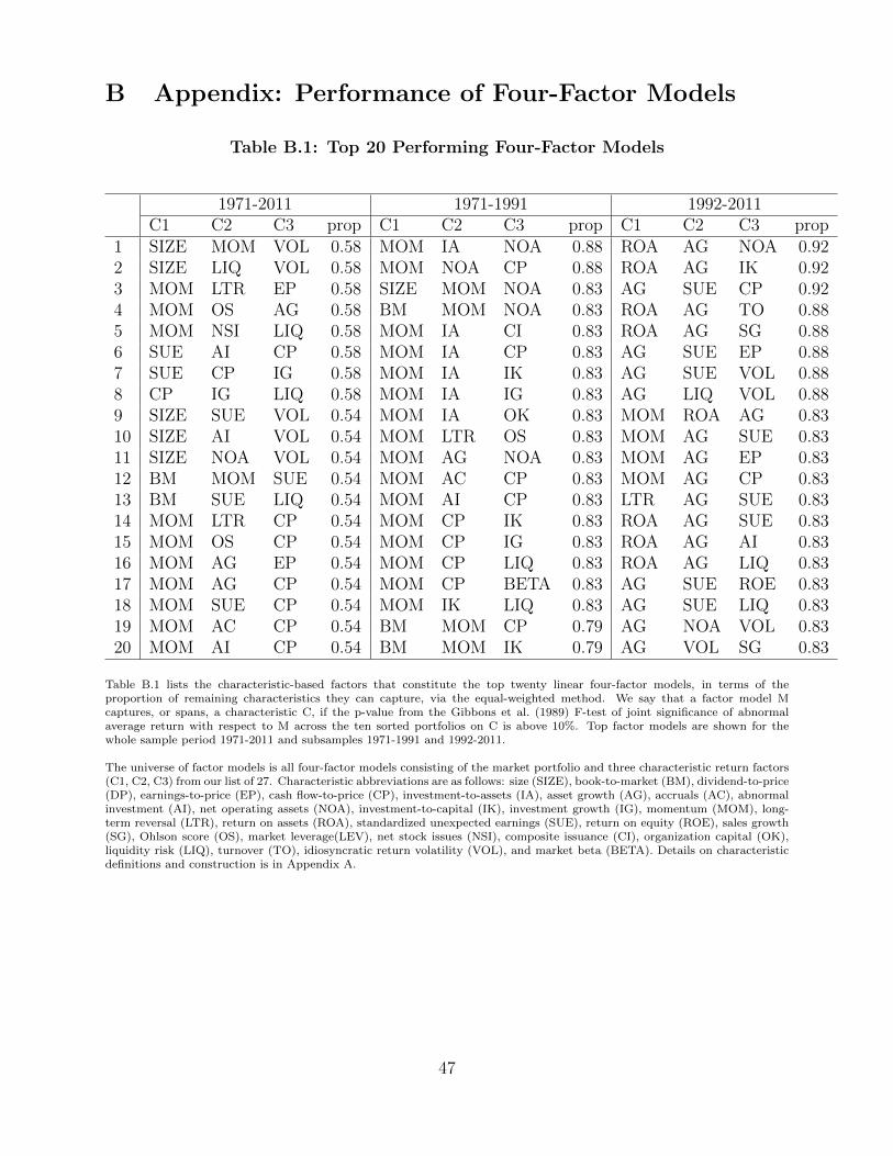
B Appendix: Performance of Four-Factor Models

Table B.1: Top 20 Performing Four-Factor Models

1971-2011 1971-1991 1992-2011C1 C2 C3 prop C1 C2 C3 prop C1 C2 C3 prop

1 SIZE MOM VOL 0.58 MOM IA NOA 0.88 ROA AG NOA 0.922 SIZE LIQ VOL 0.58 MOM NOA CP 0.88 ROA AG IK 0.923 MOM LTR EP 0.58 SIZE MOM NOA 0.83 AG SUE CP 0.924 MOM OS AG 0.58 BM MOM NOA 0.83 ROA AG TO 0.885 MOM NSI LIQ 0.58 MOM IA CI 0.83 ROA AG SG 0.886 SUE AI CP 0.58 MOM IA CP 0.83 AG SUE EP 0.887 SUE CP IG 0.58 MOM IA IK 0.83 AG SUE VOL 0.888 CP IG LIQ 0.58 MOM IA IG 0.83 AG LIQ VOL 0.889 SIZE SUE VOL 0.54 MOM IA OK 0.83 MOM ROA AG 0.8310 SIZE AI VOL 0.54 MOM LTR OS 0.83 MOM AG SUE 0.8311 SIZE NOA VOL 0.54 MOM AG NOA 0.83 MOM AG EP 0.8312 BM MOM SUE 0.54 MOM AC CP 0.83 MOM AG CP 0.8313 BM SUE LIQ 0.54 MOM AI CP 0.83 LTR AG SUE 0.8314 MOM LTR CP 0.54 MOM CP IK 0.83 ROA AG SUE 0.8315 MOM OS CP 0.54 MOM CP IG 0.83 ROA AG AI 0.8316 MOM AG EP 0.54 MOM CP LIQ 0.83 ROA AG LIQ 0.8317 MOM AG CP 0.54 MOM CP BETA 0.83 AG SUE ROE 0.8318 MOM SUE CP 0.54 MOM IK LIQ 0.83 AG SUE LIQ 0.8319 MOM AC CP 0.54 BM MOM CP 0.79 AG NOA VOL 0.8320 MOM AI CP 0.54 BM MOM IK 0.79 AG VOL SG 0.83

Table B.1 lists the characteristic-based factors that constitute the top twenty linear four-factor models, in terms of theproportion of remaining characteristics they can capture, via the equal-weighted method. We say that a factor model Mcaptures, or spans, a characteristic C, if the p-value from the Gibbons et al. (1989) F-test of joint significance of abnormalaverage return with respect to M across the ten sorted portfolios on C is above 10%. Top factor models are shown for thewhole sample period 1971-2011 and subsamples 1971-1991 and 1992-2011.

The universe of factor models is all four-factor models consisting of the market portfolio and three characteristic return factors(C1, C2, C3) from our list of 27. Characteristic abbreviations are as follows: size (SIZE), book-to-market (BM), dividend-to-price(DP), earnings-to-price (EP), cash flow-to-price (CP), investment-to-assets (IA), asset growth (AG), accruals (AC), abnormalinvestment (AI), net operating assets (NOA), investment-to-capital (IK), investment growth (IG), momentum (MOM), long-term reversal (LTR), return on assets (ROA), standardized unexpected earnings (SUE), return on equity (ROE), sales growth(SG), Ohlson score (OS), market leverage(LEV), net stock issues (NSI), composite issuance (CI), organization capital (OK),liquidity risk (LIQ), turnover (TO), idiosyncratic return volatility (VOL), and market beta (BETA). Details on characteristicdefinitions and construction is in Appendix A.

47

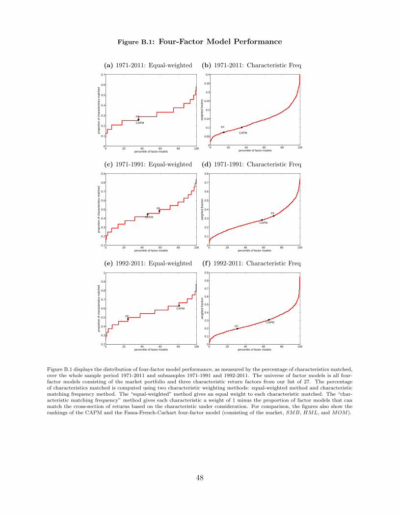
Figure B.1: Four-Factor Model Performance


0 20 40 60 80 1000

0.1

0.2

0.3

0.4

0.5

0.6

0.7

CAPM

FF


prop

ortio

n of

cha

ract

eris

tics

mat

ched


0 20 40 60 80 1000

0.05

0.1

0.15

0.2

0.25

0.3

0.35

0.4

CAPM

FF


wei

ghte

d fr

actio

n


0 20 40 60 80 1000.1

0.2

0.3

0.4

0.5

0.6

0.7

0.8

0.9

CAPM

FF


prop

ortio

n of

cha

ract

eris

tics

mat

ched


0 20 40 60 80 1000

0.1

0.2

0.3

0.4

0.5

0.6

0.7

0.8

CAPM

FF


wei

ghte

d fr

actio

n


0 20 40 60 80 1000.2

0.3

0.4

0.5

0.6

0.7

0.8

0.9

1

CAPM

FF


prop

ortio

n of

cha

ract

eris

tics

mat

ched


0 20 40 60 80 1000

0.1

0.2

0.3

0.4

0.5

0.6

0.7

0.8

0.9

CAPMFF


wei

ghte

d fr

actio

n

Figure B.1 displays the distribution of four-factor model performance, as measured by the percentage of characteristics matched,over the whole sample period 1971-2011 and subsamples 1971-1991 and 1992-2011. The universe of factor models is all four-factor models consisting of the market portfolio and three characteristic return factors from our list of 27. The percentageof characteristics matched is computed using two characteristic weighting methods: equal-weighted method and characteristicmatching frequency method. The “equal-weighted” method gives an equal weight to each characteristic matched. The “char-acteristic matching frequency” method gives each characteristic a weight of 1 minus the proportion of factor models that canmatch the cross-section of returns based on the characteristic under consideration. For comparison, the figures also show therankings of the CAPM and the Fama-French-Carhart four-factor model (consisting of the market, SMB, HML, and MOM).

48

Figure B.2: Four-Factor Model Performance

Figure B.2 shows a heatmap matrix representation of overall factor model performance. The universe of factor models is allfour-factor models consisting of the market portfolio and three characteristic return factors from our list of 27. Factors are thehigh minus low portfolio from sorting firms into ten portfolios with respect to the underlying firm characteristic. Factor modelsare ordered along the x-axis in increasing proportion of characteristics matched; characteristics are ordered along the y-axis indecreasing frequency matched (listed in parentheses). Cell (i, j) is shaded black if factor model i is able to match characteristicj, shaded gray if factor model i is unable to match characteristic j, and shaded white if factor model i comprises of a factorconstructed from characteristic j. We present figures for the whole sample period 1971-2011 and subsamples 1971-1991 and1992-2011.


(a) 1971-2011

Cha

ract

eris

tic


MOM(0.00)IA(0.00)CI(0.00)

VOL(0.00)IG(0.00)

SIZE(0.00)AC(0.01)AG(0.02)OS(0.02)NSI(0.02)

SUE(0.03)NOA(0.07)LTR(0.07)

AI(0.10)EP(0.12)LIQ(0.26)CP(0.33)IK(0.42)

ROA(0.50)BM(0.61)OK(0.63)

LEV(0.68)DP(0.79)

ROE(0.84)TO(0.90)SG(0.90)

BETA(0.91)

49

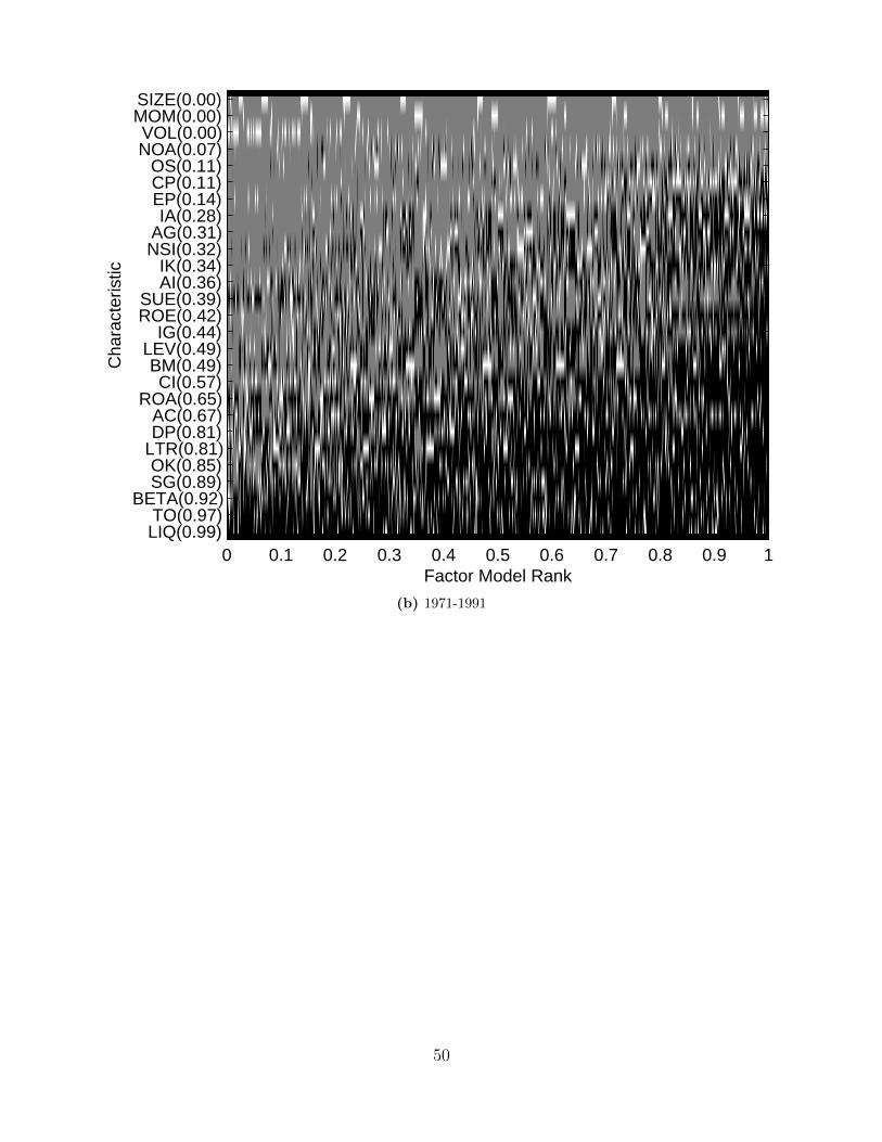
Cha

ract

eris

tic


SIZE(0.00)MOM(0.00)VOL(0.00)NOA(0.07)

OS(0.11)CP(0.11)EP(0.14)IA(0.28)

AG(0.31)NSI(0.32)

IK(0.34)AI(0.36)

SUE(0.39)ROE(0.42)

IG(0.44)LEV(0.49)BM(0.49)CI(0.57)

ROA(0.65)AC(0.67)DP(0.81)

LTR(0.81)OK(0.85)SG(0.89)

BETA(0.92)TO(0.97)LIQ(0.99)

(b) 1971-1991

50

Cha

ract

eris

tic


LTR(0.00)AG(0.01)

SUE(0.01)IG(0.04)CI(0.09)

NSI(0.14)TO(0.14)EP(0.28)

VOL(0.35)AI(0.45)

SIZE(0.48)ROA(0.49)

IA(0.52)AC(0.53)OK(0.58)OS(0.67)

NOA(0.74)CP(0.79)

MOM(0.83)SG(0.87)

ROE(0.91)LIQ(0.98)

IK(1.00)DP(1.00)

BETA(1.00)BM(1.00)

LEV(1.00)

(c) 1992-2011

51

C Appendix: Performance of Three-Factor Models Formed

Over the Largest 80 % of Firms

Table C.1: Model Performance Correlation: Largest 80% of Firms

1971-2011 1971-1991 1992-2011Method rank corr corr rank corr corr rank corr corrEqual-weighted 0.67 0.70 0.78 0.81 0.69 0.72Characteristic Freq 0.61 0.66 0.70 0.78 0.67 0.65

Table C.1 shows the rank correlation and correlation of factor model performance when factors are constructed from only thelargest 80% of firms versus the standard construction when we do not restrict firm size.

The universe of factor models is all three-factor models consisting of the market portfolio and two characteristic return factorsfrom our list of 27. The rank correlation is Spearman’s rank correlation coefficient from the ranking of factor models, basedon the percentage of characteristics matched. The correlation is the correlation coefficient of factor models’ percentage ofcharacteristics matched.

Correlations are shown for two characteristic weighting methods, equal-weighted method and characteristic matching frequencymethod, as well as for the whole sample period 1971-2011 and subsamples 1971-1991 and 1992-2011. The “equal-weighted”method gives an equal weight to each characteristic matched. The “characteristic matching frequency” method gives eachcharacteristic a weight of 1 minus the proportion of factor models that can match the cross-section of returns based on thecharacteristic under consideration.

52

Table C.2: Characteristics Factors: Summary Statistics - Largest 80% of FirmsTable C.2 contains the monthly value-weighted average returns, CAPM alphas, and Fama-French alphas for the 27 characteristic-based return factors, over the whole and subsample periods. Factors are the high minus low portfolio from sorting the largest80% of firms into ten portfolios with respect to the underlying firm characteristic. Abbreviations: size (SIZE), book-to-market(BM), dividend-to-price (DP), earnings-to-price (EP), cash flow-to-price (CP), investment-to-assets (IA), asset growth (AG),accruals (AC), abnormal investment (AI), net operating assets (NOA), investment-to-capital (IK), investment growth (IG),momentum (MOM), long-term reversal (LTR), return on assets (ROA), standardized unexpected earnings (SUE), return onequity (ROE), sales growth (SG), Ohlson score (OS), market leverage (LEV), net stock issues (NSI), composite issuance (CI),organization capital (OK), liquidity risk (LIQ), turnover (TO), idiosyncratic volatility (VOL), and market beta (BETA).

Panel A: Average Returns1971-2011 1971-1991 1992-2011

Characteristic ret t stat ret t stat ret t statSIZE -0.002 -0.87 0.002 0.48 -0.006 -1.55BM 0.005 2.35 0.005 1.53 0.005 1.87DP 0.002 0.96 0.002 0.58 0.003 0.78EP 0.005 2.30 0.008 2.95 0.002 0.64CP 0.009 3.51 0.012 4.24 0.005 1.32IA -0.007 -4.31 -0.007 -3.10 -0.007 -2.98AG -0.007 -3.44 -0.006 -2.27 -0.008 -2.58AC -0.005 -2.84 -0.004 -1.62 -0.007 -2.38AI -0.002 -1.09 0.000 -0.21 -0.003 -1.22NOA 0.001 0.23 0.003 0.81 -0.001 -0.29IK -0.003 -1.19 -0.004 -1.48 -0.003 -0.50IG -0.004 -2.26 -0.003 -1.72 -0.005 -1.59MOM 0.016 4.22 0.021 5.28 0.010 1.58LTR -0.003 -1.28 -0.002 -0.56 -0.005 -1.22ROA 0.009 2.86 0.007 2.15 0.010 2.00SUE 0.001 0.71 0.007 3.26 -0.005 -1.72ROE 0.002 0.63 0.003 1.12 0.000 0.04SG -0.002 -1.14 -0.003 -1.14 -0.002 -0.53OS -0.008 -2.40 -0.008 -2.09 -0.008 -1.47LEV 0.004 1.69 0.003 0.92 0.005 1.47NSI -0.005 -3.94 -0.006 -3.96 -0.005 -2.09CI -0.005 -2.83 -0.005 -1.82 -0.006 -2.17OK -0.002 -0.57 -0.001 -0.37 -0.002 -0.44LIQ 0.004 1.93 0.002 0.60 0.006 2.11TO -0.001 -0.48 -0.002 -0.47 -0.001 -0.26VOL -0.012 -3.00 -0.018 -4.76 -0.006 -0.80BETA -0.001 -0.18 -0.001 -0.22 -0.001 -0.08

53

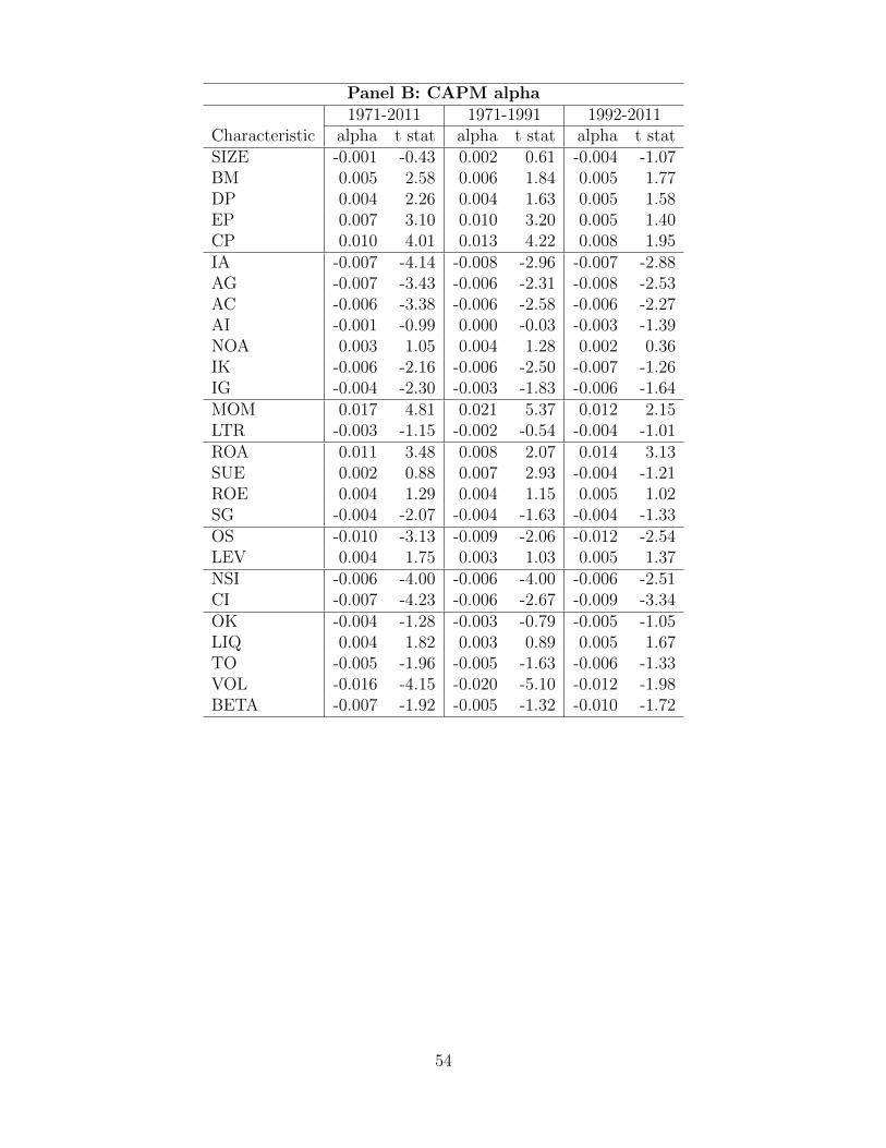
Panel B: CAPM alpha1971-2011 1971-1991 1992-2011

Characteristic alpha t stat alpha t stat alpha t statSIZE -0.001 -0.43 0.002 0.61 -0.004 -1.07BM 0.005 2.58 0.006 1.84 0.005 1.77DP 0.004 2.26 0.004 1.63 0.005 1.58EP 0.007 3.10 0.010 3.20 0.005 1.40CP 0.010 4.01 0.013 4.22 0.008 1.95IA -0.007 -4.14 -0.008 -2.96 -0.007 -2.88AG -0.007 -3.43 -0.006 -2.31 -0.008 -2.53AC -0.006 -3.38 -0.006 -2.58 -0.006 -2.27AI -0.001 -0.99 0.000 -0.03 -0.003 -1.39NOA 0.003 1.05 0.004 1.28 0.002 0.36IK -0.006 -2.16 -0.006 -2.50 -0.007 -1.26IG -0.004 -2.30 -0.003 -1.83 -0.006 -1.64MOM 0.017 4.81 0.021 5.37 0.012 2.15LTR -0.003 -1.15 -0.002 -0.54 -0.004 -1.01ROA 0.011 3.48 0.008 2.07 0.014 3.13SUE 0.002 0.88 0.007 2.93 -0.004 -1.21ROE 0.004 1.29 0.004 1.15 0.005 1.02SG -0.004 -2.07 -0.004 -1.63 -0.004 -1.33OS -0.010 -3.13 -0.009 -2.06 -0.012 -2.54LEV 0.004 1.75 0.003 1.03 0.005 1.37NSI -0.006 -4.00 -0.006 -4.00 -0.006 -2.51CI -0.007 -4.23 -0.006 -2.67 -0.009 -3.34OK -0.004 -1.28 -0.003 -0.79 -0.005 -1.05LIQ 0.004 1.82 0.003 0.89 0.005 1.67TO -0.005 -1.96 -0.005 -1.63 -0.006 -1.33VOL -0.016 -4.15 -0.020 -5.10 -0.012 -1.98BETA -0.007 -1.92 -0.005 -1.32 -0.010 -1.72

54

Panel C: Fama-French alpha1971-2011 1971-1991 1992-2011

Characteristic alpha t stat alpha t stat alpha t statSIZE 0.002 1.10 0.005 2.60 -0.001 -0.54BM 0.000 -0.08 -0.002 -1.25 0.001 0.63DP 0.000 0.22 -0.002 -0.83 0.002 0.66EP 0.007 3.10 0.010 3.40 0.004 1.43CP 0.007 3.01 0.008 2.77 0.006 2.19IA -0.005 -3.17 -0.004 -1.90 -0.006 -2.42AG -0.003 -1.88 -0.001 -0.80 -0.005 -1.82AC -0.006 -3.37 -0.005 -2.50 -0.007 -2.24AI -0.001 -0.53 0.001 0.40 -0.002 -1.04NOA 0.001 0.41 0.003 1.37 -0.001 -0.37IK 0.000 -0.21 -0.001 -0.61 0.000 -0.14IG -0.002 -1.01 -0.001 -0.78 -0.002 -0.81MOM 0.019 5.55 0.023 6.24 0.014 2.43LTR 0.002 1.10 0.005 1.74 0.001 0.27ROA 0.012 4.28 0.012 4.57 0.014 3.61SUE 0.003 1.49 0.010 4.43 -0.003 -1.04ROE 0.005 1.87 0.009 3.82 0.004 1.00SG -0.001 -0.59 -0.001 -0.32 -0.001 -0.68OS -0.011 -4.65 -0.012 -4.70 -0.012 -3.85LEV -0.002 -1.43 -0.004 -1.89 -0.001 -0.24NSI -0.005 -3.28 -0.005 -2.92 -0.006 -2.53CI -0.006 -3.76 -0.004 -2.33 -0.007 -2.96OK -0.001 -0.66 -0.001 -0.56 -0.002 -0.66LIQ 0.003 1.43 0.000 0.14 0.005 1.78TO -0.001 -0.53 -0.002 -0.78 -0.001 -0.34VOL -0.016 -5.63 -0.022 -7.97 -0.011 -2.68BETA -0.003 -1.01 -0.002 -0.56 -0.006 -1.36

55

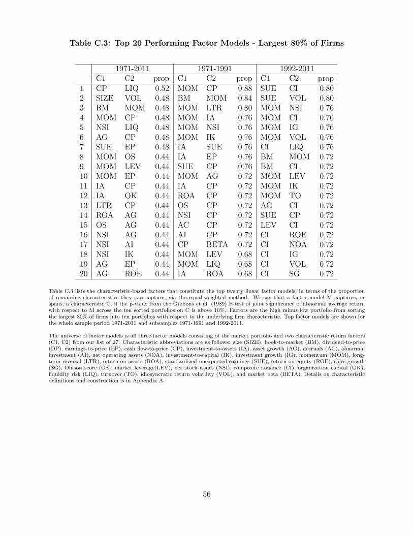
Table C.3: Top 20 Performing Factor Models - Largest 80% of Firms


1 CP LIQ 0.52 MOM CP 0.88 SUE CI 0.802 SIZE VOL 0.48 BM MOM 0.84 SUE VOL 0.803 BM MOM 0.48 MOM LTR 0.80 MOM NSI 0.764 MOM CP 0.48 MOM IA 0.76 MOM CI 0.765 NSI LIQ 0.48 MOM NSI 0.76 MOM IG 0.766 AG CP 0.48 MOM IK 0.76 MOM VOL 0.767 SUE EP 0.48 IA SUE 0.76 CI LIQ 0.768 MOM OS 0.44 IA EP 0.76 BM MOM 0.729 MOM LEV 0.44 SUE CP 0.76 BM CI 0.7210 MOM EP 0.44 MOM AG 0.72 MOM LEV 0.7211 IA CP 0.44 IA CP 0.72 MOM IK 0.7212 IA OK 0.44 ROA CP 0.72 MOM TO 0.7213 LTR CP 0.44 OS CP 0.72 AG CI 0.7214 ROA AG 0.44 NSI CP 0.72 SUE CP 0.7215 OS AG 0.44 AC CP 0.72 LEV CI 0.7216 NSI AG 0.44 AI CP 0.72 CI ROE 0.7217 NSI AI 0.44 CP BETA 0.72 CI NOA 0.7218 NSI IK 0.44 MOM LEV 0.68 CI IG 0.7219 AG EP 0.44 MOM LIQ 0.68 CI VOL 0.7220 AG ROE 0.44 IA ROA 0.68 CI SG 0.72

Table C.3 lists the characteristic-based factors that constitute the top twenty linear factor models, in terms of the proportionof remaining characteristics they can capture, via the equal-weighted method. We say that a factor model M captures, orspans, a characteristic C, if the p-value from the Gibbons et al. (1989) F-test of joint significance of abnormal average returnwith respect to M across the ten sorted portfolios on C is above 10%. Factors are the high minus low portfolio from sortingthe largest 80% of firms into ten portfolios with respect to the underlying firm characteristic. Top factor models are shown forthe whole sample period 1971-2011 and subsamples 1971-1991 and 1992-2011.

The universe of factor models is all three-factor models consisting of the market portfolio and two characteristic return factors(C1, C2) from our list of 27. Characteristic abbreviations are as follows: size (SIZE), book-to-market (BM), dividend-to-price(DP), earnings-to-price (EP), cash flow-to-price (CP), investment-to-assets (IA), asset growth (AG), accruals (AC), abnormalinvestment (AI), net operating assets (NOA), investment-to-capital (IK), investment growth (IG), momentum (MOM), long-term reversal (LTR), return on assets (ROA), standardized unexpected earnings (SUE), return on equity (ROE), sales growth(SG), Ohlson score (OS), market leverage(LEV), net stock issues (NSI), composite issuance (CI), organization capital (OK),liquidity risk (LIQ), turnover (TO), idiosyncratic return volatility (VOL), and market beta (BETA). Details on characteristicdefinitions and construction is in Appendix A.

56

Table C.4: Bottom 20 Performing Factor Models - Largest 80% of Firms


1 ROA CI 0.20 ROA CI 0.24 SIZE SUE 0.362 OS OK 0.20 OS VOL 0.24 SIZE LEV 0.363 DP SUE 0.20 SUE VOL 0.24 SIZE NOA 0.364 DP AC 0.20 CI ROE 0.24 SIZE IK 0.365 DP ROE 0.20 CI OK 0.24 SIZE IG 0.366 DP VOL 0.20 ROE OK 0.24 SIZE BETA 0.367 DP TO 0.20 ROE VOL 0.24 IA LTR 0.368 DP BETA 0.20 IG VOL 0.24 IA SUE 0.369 CI VOL 0.20 LIQ VOL 0.24 IA AC 0.3610 ROE TO 0.20 VOL SG 0.24 IA IK 0.3611 ROE BETA 0.20 MOM VOL 0.20 IA BETA 0.3612 IK VOL 0.20 ROA VOL 0.20 SIZE LTR 0.3213 OK BETA 0.20 DP VOL 0.20 SIZE DP 0.3214 SG BETA 0.20 CI VOL 0.20 SIZE ROE 0.3215 SIZE MOM 0.16 AC VOL 0.20 SIZE AI 0.3216 SIZE SUE 0.16 OK VOL 0.20 IA AI 0.3217 SIZE AI 0.16 VOL TO 0.20 IA NOA 0.3218 NSI VOL 0.16 VOL BETA 0.20 IA SG 0.3219 SIZE AC 0.12 BM VOL 0.16 IA DP 0.2820 ROA VOL 0.12 LEV VOL 0.16 SIZE IA 0.20

Table C.4 lists the characteristic-based factors that constitute the bottom twenty linear factor models, in terms of theproportion of remaining characteristics they can capture, via the equal-weighted method. We say that a factor model Mcaptures, or spans, a characteristic C, if the p-value from the Gibbons et al. (1989) F-test of joint significance of abnormalaverage return with respect to M across the ten sorted portfolios on C is above 10%. Factors are the high minus low portfoliofrom sorting the largest 80% of firms into ten portfolios with respect to the underlying firm characteristic. Bottom factormodels are shown for the whole sample period 1971-2011 and subsamples 1971-1991 and 1992-2011.


57

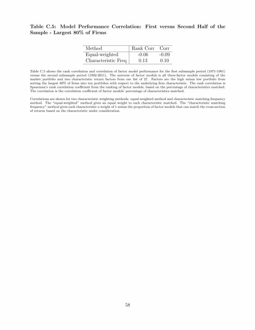
Table C.5: Model Performance Correlation: First versus Second Half of theSample - Largest 80% of Firms

Method Rank Corr CorrEqual-weighted -0.06 -0.09Characteristic Freq 0.13 0.10

Table C.5 shows the rank correlation and correlation of factor model performance for the first subsample period (1971-1991)versus the second subsample period (1992-2011). The universe of factor models is all three-factor models consisting of themarket portfolio and two characteristic return factors from our list of 27. Factors are the high minus low portfolio fromsorting the largest 80% of firms into ten portfolios with respect to the underlying firm characteristic. The rank correlation isSpearman’s rank correlation coefficient from the ranking of factor models, based on the percentage of characteristics matched.The correlation is the correlation coefficient of factor models’ percentage of characteristics matched.

Correlations are shown for two characteristic weighting methods: equal-weighted method and characteristic matching frequencymethod. The “equal-weighted” method gives an equal weight to each characteristic matched. The “characteristic matchingfrequency” method gives each characteristic a weight of 1 minus the proportion of factor models that can match the cross-sectionof returns based on the characteristic under consideration.

58

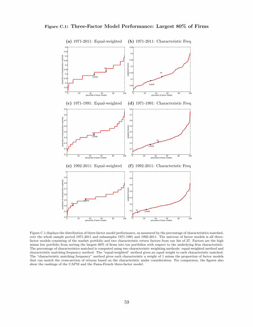
Figure C.1: Three-Factor Model Performance: Largest 80% of Firms


0 20 40 60 80 1000.1

0.15

0.2

0.25

0.3

0.35

0.4

0.45

0.5

0.55

0.6

CAPM

FF


prop

ortio

n of

cha

ract

eris

tics

mat

ched


0 20 40 60 80 1000

0.05

0.1

0.15

0.2

0.25

0.3

0.35

CAPM

FF


wei

ghte

d fr

actio

n


0 20 40 60 80 1000.1

0.2

0.3

0.4

0.5

0.6

0.7

0.8

0.9

CAPM

FF


prop

ortio

n of

cha

ract

eris

tics

mat

ched


0 20 40 60 80 1000

0.1

0.2

0.3

0.4

0.5

0.6

0.7

0.8

CAPM

FF


wei

ghte

d fr

actio

n


0 20 40 60 80 1000.2

0.3

0.4

0.5

0.6

0.7

0.8

0.9

1

CAPM

FF


prop

ortio

n of

cha

ract

eris

tics

mat

ched


0 20 40 60 80 1000

0.1

0.2

0.3

0.4

0.5

0.6

0.7

CAPMFF


wei

ghte

d fr

actio

n

Figure C.1 displays the distribution of three-factor model performance, as measured by the percentage of characteristics matched,over the whole sample period 1971-2011 and subsamples 1971-1991 and 1992-2011. The universe of factor models is all three-factor models consisting of the market portfolio and two characteristic return factors from our list of 27. Factors are the highminus low portfolio from sorting the largest 80% of firms into ten portfolios with respect to the underlying firm characteristic.The percentage of characteristics matched is computed using two characteristic weighting methods: equal-weighted method andcharacteristic matching frequency method. The “equal-weighted” method gives an equal weight to each characteristic matched.The “characteristic matching frequency” method gives each characteristic a weight of 1 minus the proportion of factor modelsthat can match the cross-section of returns based on the characteristic under consideration. For comparison, the figures alsoshow the rankings of the CAPM and the Fama-French three-factor model.

59

Figure C.2: Three-Factor Model Performance: Largest 80% of Firms

Figure C.2 shows a heatmap matrix representation of overall factor model performance. The universe of factor models is allthree-factor models consisting of the market portfolio and two characteristic return factors from our list of 27. Factors arethe high minus low portfolio from sorting the largest 80% of firms into ten portfolios with respect to the underlying firmcharacteristic. Factor models are ordered along the x-axis in increasing proportion of characteristics matched; characteristicsare ordered along the y-axis in decreasing frequency matched (listed in parentheses). Cell (i, j) is shaded black if factor modeli is able to match characteristic j, shaded gray if factor model i is unable to match characteristic j, and shaded white if factormodel i comprises of a factor constructed from characteristic j. We present figures for the whole sample period 1971-2011 andsubsamples 1971-1991 and 1992-2011.


(a) 1971-2011

Cha

ract

eris

tic


MOM(0.00)IA(0.00)

OS(0.00)NSI(0.00)

CI(0.00)AI(0.00)IG(0.00)

VOL(0.00)AC(0.01)

SUE(0.02)AG(0.05)

LTR(0.06)LIQ(0.11)EP(0.17)

NOA(0.26)BM(0.27)CP(0.31)IK(0.32)

ROA(0.34)LEV(0.39)OK(0.62)

SIZE(0.80)BETA(0.92)

DP(0.93)ROE(0.94)

SG(0.94)TO(0.97)

60

Cha

ract

eris

tic


MOM(0.00)OS(0.00)

VOL(0.00)NOA(0.02)

CP(0.05)NSI(0.08)EP(0.18)

SUE(0.18)IA(0.19)AI(0.26)

BETA(0.27)CI(0.38)

SIZE(0.40)AG(0.45)BM(0.48)

IK(0.56)ROA(0.62)ROE(0.68)

IG(0.73)LEV(0.78)DP(0.84)OK(0.87)

LTR(0.88)SG(0.90)AC(0.93)LIQ(0.99)TO(1.00)

(b) 1971-1991

61

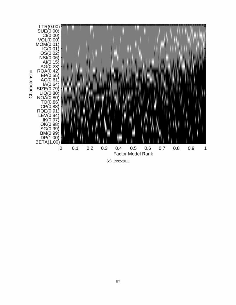
Cha

ract

eris

tic


LTR(0.00)SUE(0.00)

CI(0.00)VOL(0.00)

MOM(0.01)IG(0.01)

OS(0.02)NSI(0.06)

AI(0.15)AG(0.23)

ROA(0.42)EP(0.55)AC(0.61)IA(0.64)

SIZE(0.79)LIQ(0.80)

NOA(0.80)TO(0.86)CP(0.88)

ROE(0.91)LEV(0.94)

IK(0.97)OK(0.98)SG(0.99)BM(0.99)DP(1.00)

BETA(1.00)

(c) 1992-2011

62

european summe r sym posium in financia l … - firm characteristics... · associated with the...

Documents