european summer symposium in international macroeconomics ... · the –rm level between price and...

Euro

pean

Sum

mer

Sym

posi

um in

Inte

rnat

iona

l M

acro

econ

omic

s (E

SSIM

) 200

8

Hos

ted

by

Ban

co d

e E

spañ

a

Tarr

agon

a, S

pain

; 20-

25 M

ay 2

008

We

are

grat

eful

to th

e B

anco

de

Esp

aña

for t

heir

finan

cial

and

org

aniz

atio

nal s

uppo

rt.

Th

e vi

ews

expr

esse

d in

this

pap

er a

re th

ose

of th

e au

thor

(s) a

nd n

ot th

ose

of th

e fu

ndin

g or

gani

zatio

n(s)

or o

f CE

PR

, whi

ch ta

kes

no

inst

itutio

nal p

olic

y po

sitio

ns.

Infla

tion

dyna

mic

s w

ith S

earc

h an

d M

atch

ing

in

the

Labo

ur M

arke

t: A

Sur

vey

of A

ltern

ativ

e Sp

ecifi

catio

ns

Kai

Chr

isto

ffel,

Jam

es C

osta

in, G

rego

ry d

e W

alqu

e, K

eith

Kue

ster

, Tob

ias

Linz

ert,

S

teph

en M

illard

and

Oliv

ier P

ierra

rd

In�ation dynamics with search and matching in the

labour market: A survey of alternative

speci�cations

Kai Christo¤el, James Costain, Gregory de Walque, Keith Kuester,

Tobias Linzert, Stephen Millard and Olivier Pierrard*

May 14, 2008

Abstract

This paper reviews recent approaches to modeling the labour market, and

assesses their implications for in�ation dynamics through both their e¤ect on

marginal cost and on price-setting behavior. In a search and matching environ-

ment, we consider the following modeling setups: right-to-manage bargaining vs.

e¢ cient bargaining, wage stickiness in new and existing matches, interactions at

the �rm level between price and wage-setting, alternative forms of hiring fric-

tions, search on-the-job and endogenous job separation. In particular, we look

at the impact of these various modelling choices on the determinants of marginal

cost and in�ation dynamics, and provide the underlying intuition.

JEL Classi�cation System: E31,E32,E24,J64

Keywords: In�ation Dynamics, Labour Market, Business Cycle, Real Rigidities.

*Correspondence and a¢ liations: Christo¤el, Kuester and Linzert: European Central Bank, Kaiser-straße 29, 60311 Frankfurt, Germany; e-mail: kai.christo¤[email protected], [email protected], [email protected]. Costain: División de Investigación, Servicio de Estudios, Banco de España, CalleAlcalá 50, E-28014 Madrid; email: [email protected]. de Walque: National Bank of Belgium Re-search Department, Boulevard de Berlaymont 14, B-1000 Brussels, email: [email protected]: Bank of England, Threadneedle Street, London EC2R 8AH, UK, email: [email protected]. Pierrard: Banque Centrale du Luxembourg, 2, boulevard Royal, L-2983 Lux-embourg, email: [email protected].

Without implication, we would like to thank Raf Wouters for taking the initiative in suggesting thisproject and participants in the Eurosystem Wage Dynamics Network for helpful comments. The WageDynamics Network is a joint research network by the ECB and Eurosystem national central banks.The views expressed in this paper are those of the authors and do not necessarily re�ect the views heldby the European Central Bank, any other central bank in the Eurosystem or the Bank of England.

1

1 Introduction and motivation

Central banks are typically charged with maintaining price stability, often de�ned by

a target for in�ation. But in order to achieve this, it is important to understand what

the dynamics of in�ation are: in particular, what are the nature of nominal and real

frictions associated with the adjustments of prices in the economy and how do these

frictions a¤ect the response of in�ation to shocks. The answer to this question will

have an important bearing for the monetary transmission mechanism as well as what

a central bank can and should seek to achieve.

A long tradition in monetary economics assigned labour market frictions and, in par-

ticular wage-setting frictions, a central role in in�ation dynamics; see, e.g., Ball and

Romer (1990), Christiano et al. (2005). The rationale was that labour market fric-

tions altered either aggregate marginal cost or the �rms�price-setting behaviour for

given marginal cost.1 An active strand of research has recently set out to model the

labour market more explicitly in a New Keynesian environment, most often opting for

variants of the Mortensen and Pissarides (1994) model of search and matching fric-

tions. The variety of implications is stunning. Some have, for example, argued that

accounting for equilibrium unemployment increases the resilience of marginal cost, and

hence in�ation, to shocks by adding a pool of slack resources; see, e.g., Trigari (2005)

and Walsh (2005). Others, e.g., Krause and Lubik (2007), conclude that contrary to

received wisdom wage rigidity does not impact on in�ation inertia.2

This paper surveys the existing modeling approaches. It explains their implications

for the behavior of marginal cost and in�ation, and highlights which of the particular

features of each modeling approach drive the results. A key aim is to give a structure

to the rich variety of existing literature, and to distill the policy-relevant features.3

Technically, we take a plain New Keynesian model with search and matching frictions as

our starting point. As the baseline, we choose the e¢ cient bargaining version of Trigari

(2006). Building on this, we replace certain assumptions on the labor market structure

by others, one at a time. We consider the following variants: right-to-manage (instead

of e¢ cient) bargaining (Trigari, 2006), stickiness of wages in these setups (Gertler and

Trigari, 2006; Christo¤el and Linzert, 2005) di¤erentiating between stickiness in new

1Thus, the labour market was seen as a source of �real rigidities�. For an overview of the extensiveliterature on real rigidities more generally, see Woodford (2003).

2Another strand of iterature has been concerned with normative implications, such as the designof optimal monetary policy; see, e.g., Blanchard and Gali (2006), Faia (2008), Tang (2006).

3Other papers, largely sparked by Shimer�s (2005) critique, seek to improve the modeling or cal-ibration of the labour market per se, and are not necessarily concerned with nominal frictions, e.g.,Gertler and Trigari (2006), Fujita and Ramey (2005), Yashiv (2006). In this paper, we take up someof the suggestions made in these papers, as �through their implications for the behavior of wages and(un)employment �they also imply changes in the behavior of marginal cost.

2

matches and existing matches (Bodart et al., 2005; Bodart et al., 2006), interactions at

the �rm-level between price and wage-setting (Kuester, 2007; Sveen and Weinke, 2007;

Thomas, 2008), alternative forms of vacancy posting costs (Yashiv, 2006) and the hiring

process (Fujita and Ramey, 2005), search on-the-job (Krause and Lubik, 2006; van

Zandweghe, 2006) and endogenous separation (den Haan et al., 2000; Zanetti, 2007).

In particular, we look at the impact of these variants on marginal cost and in�ation.

In each of the cases we provide intuition for the e¤ect that a speci�c modi�cation of

the baseline model has on in�ation dynamics.

In the New Keynesian model, the response of in�ation to a given shock (such as a

monetary policy shock) is determined both by the response of real marginal cost to

that shock and by the reactions of �rms to a given change in real marginal cost.

Models that imply large and immediate responses of real (marginal) wages to shocks

will not match the sluggish response of in�ation observed in empirical research (see

Appendix A for a summary) unless other real rigidities induce �rms not to pass such

changes in costs through to their customers, or unless real wages do not fully drive all

of marginal cost. For this reason, throughout the paper, we trace the impact of the

respective modeling approach on the form and behaviour of marginal cost and on the

�rms�price setting behaviour and analyse in which respect each approach improves

upon the standard New Keynesian framework in accounting for a sluggish response of

in�ation to monetary shocks.

Our �ndings are as follows. We show, �rst, that the baseline model predicts a response

of in�ation that is too large relative to the data, as a result of the large and immediate

response of real marginal cost. This would suggest either that the labour market is

not an important source of real rigidities or that the speci�c way of modeling the

labour market was not appropriate. Indeed, when combined with a �right-to-manage�

assumption for the determination of hours, staggered wages at the level of the match

help to smooth the reaction of the marginal wage resulting in a smaller response to

shocks of marginal cost and in�ation. In�ation responds even less to shocks when

accounting for the �rm-speci�c nature of labour in the search and matching model.

This, however, also had implications for the response of unemployment and vacancies

that took it further away from the data in these dimentions. While variations of the

hiring costs empirically only had a small impact on in�ation dynamics, we found that

both search on-the-job and endogenous separation reduce the response of in�ation to

shocks, though our results based on endogenous job destruction depended critically on

the calibration of the model.

The rest of the paper is structured as follows. In section 2, we lay out the baseline

model, which is Trigari�s (2006) e¢ cient bargaining setup. We highlight which are the

3

features of the model that will be changed subsequently. In section 3, we calibrate the

baseline model using euro area data and compare the responses of in�ation (and wages

and unemployment) to a monetary policy shock in the model with the responses to the

same shock in euro area data. Subsequently, we assess to which extent this response is

an artefact of the modeling approach, and assess whether other speci�cations reverse

that �nding. In section 4 we consider the e¤ects of having �right-to-manage�bargaining

and section 5 adds nominal wage rigidities for new and existing jobs, exploring how

these rigidities interact with the bargaining scheme. Section 6 considers what happens

if wages and prices are set simultaneously in the presence of �rm-speci�c labour. Section

7 allows for new hires being productive immediately and not only with a one-period

delay. In section 8 we discuss the e¤ects of varying the free-entry condition and vacancy

costs. Sections 9 and 10 consider other margins along which adjustment can occur in

the labour market: section 9 discussing on-the-job search and section 10 discussing

endogenous job destruction. Section 11 concludes. An appendix presents empirical

evidence on monetary transmission in the euro area.

2 The baseline model

In this section we lay out those aspects which we use as our baseline for the analysis.

The baseline is a simpli�ed version of Trigari�s (2006) e¢ cient bargaining setup. Some

of these aspects will remain �xed throughout the analysis, while some will be replaced

by other modeling assumptions. We point to the dimensions in which we vary the

baseline as we proceed.

2.1 Households, consumption and saving

We assume that there is a continuum of workers indexed by j on the unit interval who

supply a homogeneous type of labour. Only a proportion nt of them are employed. We

adopt a representative �or large�household interpretation so that the unemployment

rate ut is identical at the household or at the aggregate level. As shown by Merz

(1995), the representative household assumption amounts to allowing for the existence

of state contingent securities o¤ering workers insurance against di¤erences in their

speci�c labour income. Household members (workers) share their labour income, i.e.,

wage and unemployment bene�ts, before choosing per capita consumption and bond

holdings.

The representative household�s total real income is therefore equal to the aggregate

income

Yt = nt � wt � ht + (1� nt) � b+t . (1)

4

Labour income is made of the sum of hourly wages and unemployment bene�t b,

weighted by total hours worked and unemployment, respectively.4 As shareholders,

households also receive the pro�ts t generated by the monopolistic competitive retail

�rms and the intermediate producers fo labor services.

Workers hold their �nancial wealth in the form of bonds Bt. Bonds are one-period

securities with price 1=rt, where rt is the nominal interest rate. The budget constraint

faced by the representative household may be written as

Btrt � pt

+ ct + tt =Bt�1pt

+ Yt (2)

where ct represents aggregate consumption, tt are lump-sum taxes payable and pt is

the consumer price index.

We assume separability between leisure and consumption in the instantaneous utility

function, implying that all workers share the same marginal utility of wealth and choose

the same optimal consumption, be they employed or not. A worker�s utility can be

written as

U (cjt; hjt) =c1��cjt

1� �c� �

h1+�jt

1 + �(3)

with �c � 1; � > 0; � � 0. Let Ht(j) be the value function of worker j. If we

momentarily leave aside the labour supply decision, which is taken by the household

as a whole, worker j�s maximization program is

Ht(j) = maxcjt;Bjt+1

fU (cjt; hjt ) + � � EtHt+1(j)g

st: (2)

The worker�s optimal and saving decision coincide with those of his peers and are

derived from the following �rst order conditions:

�tpt

= � rt � Et��t+1pt+1

�, (4)

�t = c��ct . (5)

This block will not be altered in the variants that we present.

4b could alternatively be interpreted as the income generated by the domestic activities of anunemployed worker.

5

2.2 Firms

The baseline is a three sector economy. Firms in the �nal good sector, assumed to

be a competitive market, produce a homogeneous �nal good used for consumption.

The �nal homogeneous good is made from di¤erentiated goods which are produced

by monopolistic retailers. Retailers simply buy a homogeneous good from intermedi-

ate producers and transform them one for one into di¤erentiated goods at no cost.

Intermediate producers are perfectly competitive. They produce the intermediate ho-

mogeneous good with labour as the only input. They can hire at most one worker and

in order to �nd him/her, they post vacancies.

Final good sectorWe assume a continuum of di¤erentiated goods indexed by i on the unit interval. Final

good �rms aggregate the di¤erentiated goods yrt (i) produced by the retailers using a

Dixit-Stiglitz technology

yt =

�Z 1

0

[yrt (i)]�p di

�1=�pwith �p 2 (0; 1) (6)

where 1=�p represents the retailers�gross price mark-up while 1=(1 � �p) is the elas-

ticity of substitution between intermediate di¤erentiated goods. Each �nal good �rm

maximises pro�t, leading to the following demand for intermediate good i

yrt (i) =

�pt(i)

pt

� 1�p�1

yt (7)

where pt is the �nal good price, obtained by aggregation of the retailers prices

pt =

�Z 1

0

[pt(i)]�p

�p�1 di

��p�1�p

. (8)

The modeling of the �nal good sector will remain �xed throughout the paper.

Monopolistic retailers and price settingGiven the demand yrt (i) retail �rm i faces for its product, it buys a homogeneous

intermediate labour good at nominal price ptxt per unit and transforms it one for one

into a di¤erentiated product. Its real pro�t is

rt (i) =pt(i)� ptxt

pt� yrt (i)

At each period, a fraction 1��p of retail �rms sets a new price p�t (i). This price prevails

6

j periods later with probability �jp. The price setting �rms maximise the discounted

�ows of expected real pro�ts using a discount rate consistent with the pricing kernel

for nominal returns used by the shareholders-households. All the price setting �rms

face the same optimization problem, implying that they all choose the same new price

p�t . Pro�t maximization results in the following �rst-order condition

Et1Xj=0

��p�j � �t+j

�t�yrt+j(i)

pt+j��p�t �

1

�ppt+jxt+j

�= 0 (9)

Given the de�nition of the price index (8), its law of motion is

p

�p�p�1t = (1� �p) � (p�t )

�p�p�1 + �p � p

�p�p�1t�1 (10)

Combining (9) and (10) and log-linearising the resulting expressions around steady

state enables us to derive the New Keynesian Phillips Curve

�̂t = �Et�̂t+1 +

�1� �p

� �1� ��p

��p

x̂t , (11)

where �t = pt=pt�1 is the in�ation rate while hats denote percentage deviations from

steady state. This expression makes clear that, for a given response of in�ation to

movements in real marginal cost �which will depend on �p �the response of in�ation to

a given shock will depend on how real marginal cost responds to that shock. Within

the period of the shock, output can only be increased by increasing the number of

hours worked per worker; so the cost of increasing hours worked will determine the

immediate response of in�ation to shocks.

One-worker intermediate labor�services �rmsIn the baseline, we consider a continuum of intermediate producers uniformly distrib-

uted and selling their output in a competitive market. Their only factor of production

is labour, and labour e¢ ciency is decreasing with hours, so that h hours supplied by

one worker produce only h� units of e¢ cient labour, � < 1. Keeping the Mortensen

and Pissarides (1999) assumption, intermediate producers can hire at most one worker

so that their production is either zero or

ylt(o) = [ht(o)]� with � < 1 ,

where o indicates match o. As will be clear later, as long as wages are �exible, every

�rm pays the same wage which implies the same working time. We defer the wage

bargaining to the next section. In the baseline the labor-services sector and price-

7

setting �rms are linked through competive markets for the labor service. In section 6,

we assess the implications for in�ation dynamics once these two sectors are merged so

that there are interactions between wage and price setting at the level of the individual

�rm.

2.3 The labour market

The labor market is organized such that it links the intermediate labor-services �rm

and the workers.

Labour market �owsLet nt represent the total number of jobs. Normalising the total labour force to one

yields the following accounting identity:

nt + ut = 1 (12)

where ut denotes the number of unemployed, all of which are job-seekers. Letmt denote

the number of new �rm-worker matches. We assume that the number of matches is a

function of the number of job vacancies vt and e¤ective job seekers ut, and we consider

the following linear homogeneous matching function:

mt = �m u#t v1�#t (13)

with �m > 0 and # 2 (0; 1). Models with search on-the-job (section 9) modify the

matching function to depend also on the number of searchers on the job. In the baseline,

the probability an unemployed worker �nds a job is given by

st =mt

ut(14)

while the probability that a �rm �lls a vacancy is given by

qt =mt

vt. (15)

An exogenous proportion � of �rm-worker relationships ends each period, which implies

the following employment dynamics:

nt = (1� �) � nt�1 +mt�1 . (16)

In the baseline therefore employment is predetermined, while hours per worker are free

to adjust contemporaneously. This means that marginal costs are in the �rst period in-

8

�uenced exclusively by the marginal cost of an additional hour worked on the intensive

margin. We ease this assumption in section 7, where we allow for contemporaneous

hiring, and in section 10, which looks at endogenous separation.

Value of a job and of a vacancy for an intermediate labor-services producerThroughout the paper, �rms and workers engage in wage bargaining. This bargain-

ing distributes the rents that arise once a match is formed to both the �rm and the

worker.We denote by Jt and Vt, respectively, the asset value of a job and of a vacancy

at period t, dropping match index i for convenience:

Jt = yltxt � htwt + Et

��(1� �)

�t+1�t

Jt+1

�, (17)

Vt = �kvt + Et��t+1�t

[qtJt+1 + (1� qt)Vt+1]

�, (18)

where kvt represents the per-period hiring cost (in units of the consumption good).

Value of a job and value of unemployment for a householdFor a worker�s family, which bargains on his behalf, the value of a new job is given by

Wt = htwt ��

�t

h1+�t

1 + �+ Et

��t+1�t

[(1� �) Wt+1 + � Ut+1]

�; (19)

where Ut represents the present value of being unemployed at period t. Formally,

Ut = b+ Et

��t+1�t

[st Wt+1 + (1� st) Ut+1]

�: (20)

2.4 Wage bargaining

In this section, we discuss the bargaining over wages and hours between workers and

�rms once a match has been formed. We will focus here on a bargaining scheme that is

e¢ cient, i.e., in which the bargained wage maximizes the joint surplus of the �rm and

the worker. Also, in the baseline we abstract from any wage rigidity. We will look at a

di¤erent, right-to-manage bargaining scheme in section 4, and will analyze in section

5 what real wage rigidity means for in�ation and unemployment dynamics.

Baseline: e¢ cient bargaining over wages and hoursUnder e¢ cient bargaining, hours and wages are bargained over simultaneously and

�rms and workers maximise the joint surplus of the �rm-worker pair. As a result,

9

the decision for hours worked is independent of the wage actually set, as long as the

wage is within the bargaining set, as stressed by Hall (2005). In our model, e¢ ciency

requires that the marginal gain to the labor �rm of an additional hour worked (the

�rm�s marginal value product of labour, xtmplt) is the same as the marginal cost to

the worker of that hour (his marginal rate of substitution between consumption and

leisure, mrst). In other words, the �rm will at the margin compensate the worker

at his subjective price for work. This makes clear that this subjective price of work

determines the marginal wage and is essential for the marginal costs of producing labor

services, while the average wage rate, wt, will be unrelated to that marginal wage and,

thus, to real marginal cost.5

In particular, we assume that �rms and workers use Nash bargaining to determine both

wages and hours. The outcome of the bargaining process is obtained by maximization

of the Nash product:

maxwt;ht

(Wt � Ut)� � (Jt � Vt)

1�� : (21)

The �rst term of the Nash product is the surplus a worker obtains from a job, raised to

the worker�s relative bargaining power � 2 (0; 1). The second term is the �rm surplus,raised to the �rm�s relative bargaining power 1� �.

The �rst-order condition for wages is

� � (Jt � Vt) �dWt

dwt+ (1� �) � (Wt � Ut) �

dJtdwt

= 0 . (22)

The �rst-order condition for hours is

� � (Jt � Vt) �dWt

dht+ (1� �) � (Wt � Ut) �

dJtdht

= 0 . (23)

Combining these two optimality conditions, we get

dJtdht

� dWt

dwt=dJtdwt

� dWt

dht(24)

Under e¢ cient bargaining, the solution of (24) simpli�es to

�

�th�t = xt�h

��1t = �

xtylt

ht: (25)

5Putting it di¤erently, the average hourly wage in this bargaining setup is not a su¢ cient statisticfor the marginal wage. Fixing the average hourly wage rate leaves the marginal wage schedule stillindeterminate. This di¤ers from a the right-to-manage bargaining setup that we introduce in section4.

10

This shows that the individual matches�wage is not allocational for hours, that is

@ht=@wt = 0. Note that xt, the price of labor services, coincides with the marginal

costs of price-setting �rms. Rearranging above equation

xt =�h�t�t

�h��1t

:=mrstmplt

(26)

highlights the implications of e¢ cient bargaining for marginal costs (and in�ation).

Real marginal cost will equal the worker�s marginal rate of substitution between con-

sumption and leisure (mrst) divided by the real marginal product of labour (mplt).

Both of these will, in turn, depend on hours worked per employee. Again, the key

point is that the cost of an extra hour�s work will be given by the marginal wage, which

coincides with mrst; and not the average real wage, measured by wt.

This bargaining procedure is said to be �e¢ cient� because it results in hours that

maximise the joint surplus of the match, that is Jt+Wt�Ut�Vt. Since the wage is notallocational for hours, the �rst-order condition (22) for the wage bargaining simpli�es

to

� � (Jt � Vt) = (1� �) � (Wt � Ut) (27)

which states that each of the contracting parties receives a share of the total surplus

proportional to its relative bargaining power.

2.5 Vacancy posting

In order to �nd a worker, and so in order to produce, labor �rms have to post a vacancy

�rst. In the baseline we follow the most common assumptions in the literature, namely

that vacancy posting costs are constant over the cycle in real terms and that these costs

keep open a vacancy for just one period. Both of these assumptions will be relaxed

individually in section 8.

Baseline: free entry condition and constant recurrent vacancy posting costsIn the baseline model, we assume free entry in the market for vacancies. This implies

that in equilibrium the value of a vacancy is Vt = 0 in every period t. Furthermore,

assuming that the vacancy posting cost kvt is constant over the cycle at value �, as in

the standard Mortensen and Pissarides (1999) framework, the equation for the asset

value of a vacancy (18) can be recast as:

� = qt Et

��t+1�t

Jt+1

�. (28)

11

Total vacancy costs are given by �vt, and the average cost per hiring is �=qt. Using

this, the value of a job for a �rm simpli�es to

Jt = ylt � xt � ht � wt + (1� �) � �qt. (29)

From equations (28) and (29), one easily obtains the dynamic representation of the

average cost per hire

�

qt= Et

��t+1�t

�ylt+1 � xt+1 � ht+1 � wt+1 + (1� �) � �

qt+1

��(30)

which determines job creation in the model. Substituting (17), (19) and (20) into (27)

while taking (28) into account, we obtain the following wage equation

ht � wt = � � ylt � xt + (1� �) � �

�t� h

1+�t

1 + �+ b+

� � �1� �

� �t

!(31)

where �t = vtutrepresents labour market tightness. Intuitively, in these equations the

wage is a weighted sum of a worker�s value to the �rm �i.e., the value of his output �

and the value of his outside option �consisting of the utility he gains from his leisure,

his unemployment bene�t and the present discounted value of his expected gains from

search, which will be higher the easier it is to �nd a job (i.e., the tighter is the labour

market).6

2.6 Monetary policy, �scal policy and market clearing

Throughout the paper we assume that monetary policy is conducted according to the

following Taylor rule

r̂t = �r � r̂t�1 + (1� �r) � �� ̂t�1 + �mt (33)

whith �r � 0 and �� > 1 and �mt is an i.i.d. normally distributed interest rate shock.Lump-sum taxes, tt; are set so as to balance the budget period by period, there is no

autonomous government spending.

6Alternatively, we can use the hours equation (25) to rewrite the wage equation in a form that isuseful for eliminating hours and wages from (30):

ht � wt = ��t + (1� �)b+�� +

� (1� �)1 + �

�xty

lt (32)

12

Equilibrium in the �nal goods market implies7

yt = ct : (34)

2.7 Summary

To sum up, the baseline model consists of the following equations: (4), (5), (12), (13),

(14), (15), (16), (9), (10), (33), (34), (25), (30) and (31).

3 Stylized facts and the baseline economy

The aim of this paper is to elicit the role of speci�c labor market frictions for the

behaviour of marginal cost and in�ation. In order to obtain a measure of the empirical

relevance of the frictions, we compare the responses to a monetary policy easing in the

respective model variant to stylized facts for the euro area. We start by discussing the

calibration of the models. Thereafter we present stylized facts regarding the e¤ects of

monetary policy in the euro area (in section 3.2) and highlight the shortcomings of the

baseline model in that regard (in section 3.3).

3.1 Calibration of the model economies

In order to put all approaches on the same footing, the calibration is harmonised as

much as possible. The calibration matches salient features of the euro area between

1984 and 2006. See, e.g., Christo¤el et al. (2008) for a description of the underlying

data, further references for the calibrated values, and a comparison of the euro area

and the U.S. labour market. Table 1 presents the assigned common parameter values.

The time-discount factor, �, is chosen to match an average annual real rate of 3.3%.

We set � to 10, implying an elasticity of substitution for labour of 0.1, in line with �

but at the lower end of �microeconomic studies for the euro area.8 The value of the

risk aversion coe¢ cient is set to �c = 1:5, following Smets and Wouters (2003).

Turning to the labour good sector and the labour markets, we set � = 0:99, so there

are almost constant-returns to hours per employee.9 On monthly data ranging to

7We assume that vacancy posting costs are taxes which are rebated lump-sum to the consumersand which do not require real ressources.

8The elasticity of inter-temporal substitution of labor, 1/�, is small in most microeconomic studies(between 0 and 0.5) for the euro area, see Evers, Mooij, and Vuuren (2005) for details, who reportstatistics based on a meta sample as well as estimates based on Dutch data.

9Our model does not contain capital. In some of the variants, there is thus a trade-o¤ betweenobtaining a reasonable labour share (of around 60%) and small ex post pro�ts associated with jobs.

13

Value Explanation

Preferences� .992 Time-discount factor (matches annual real rate of 3.3 percent).� 10 Labor supply elasticity of 0.1.�c 1.5 Risk aversion.

Bargaining, Intermediate Producers and Labor Market� .99 Labor elasticity of production (close to constant-returns-to-scale).# .6 Elasticity of matches with respect to unemployment.� .5 Bargaining power of workers�w .83 Calvo stickiness wages (avg. wage duration 6 qtrs), where applicable.

Monopolistic Retail Sector and Price Setting�p 1.1 Price-markup of 10 percent.�p .75 Calvo stickiness of prices (average duration of 4 qrts).

Monetary Policy � 1.5 Response to in�ation in Taylor rule. R .85 Interest rate smoothing coe¢ cient in Taylor rule.

Table 1: Parameters and their calibrated values. The Table reports calibratedparameter values that are identical over the di¤erent modeling approaches. The model is calibratedto the euro area from 1984Q1 to 2006Q4.

the early 1990s, Burda and Wyplosz (1994) estimate an elasticity of matches with

respect to unemployment of # = 0:7 for France, Germany and Spain. Petrongolo and

Pissarides (2001) survey estimates of the matching function for European countries

and for the U.S. and conclude that a range from # = 0:5 to # = 0:7 is admissible.

We select the midpoint, setting # = 0:6. The bargaining power of workers is set to a

conventional value of � = 0:5.

For the variants that involve wage stickiness, we follow recent evidence collected by

the Eurosystem Wage Dynamics Network,du Caju et al. (2008),.which reports average

wage contract durations for various euro area countries between one and three years.

Where applicable, we therefore set the degree of nominal wage rigidity to �w = 0:83;

which implies an average wage duration of 6 quarters.

In the price-setting sector, we calibrate the markup to a conventional value of 10%,

so �p = 1=1:1 (in the Dixit-Stiglitz setup this implies a price-elasticity of demand

of � = 11). For the average contract duration of prices we use the results of the

Eurosystem In�ation Persistence Network and set the corresponding Calvo parameter

We opt to �t the latter, and choose � = 0:99 instead of a lower value.

14

to �p = 0:75, see Alvarez et al. (2005), which amounts to an average price duration of

4 quarters. As is conventional, we set the response of monetary policy to in�ation to

� = 1:5, and allow for interest rate smoothing by setting R = 0:85.

In addition to these direct parameterizations, we chose to ensure that steady state

values for certain endogenous variables coincide across the di¤erent setups. The target

values for these variables, shown Table 2, thereby implicitly de�ne the values of the

remaining model parameters.

Value Explanationu 9% Unemployment rateq 70% Probability of �nding a workerh 1 Hours worked per employee.bwh

65% Unemployment bene�ts replacement rate.� .06 Quarterly separation rate.

Table 2: Calibration Targets. The table reports cali-brated parameter values. The model is calibrated to the euro areafrom 1984Q1 to 2006Q4.

The steady state unemployment rate is targeted to be u = 9%, in line with the average

of the euro area unemployment rate over the sample 1984 to 2006. We target a

probability of �nding a worker when having opened a vacancy of q = 0:7, in line with

the euro area evidence collected in Christo¤el et al. (2008). Our target for steady state

hours worked per employee is h = 1. We set the replacement income b so as to ensure

that the replacement rate in steady state in each of the variants conforms with the

net replacement rates published by the OECD in its set of �Bene�ts and Wages�data.

This replacement rate is bwh= 65%. Finally, the evidence collected in Christo¤el et

al. (2008) and Hobijn and Sahin (2007) points.to quarterly separation rates, from a

worker �ow perspective, of � = 6%:

3.2 Stylized facts �the transmission of monetary policy

In the following, we assess each of the di¤erent modeling variants against �ve sylized

facts regarding the monetary transmission in the euro area. These facts are based on

VAR evidence that we generated ourselves, and a survey of the literature,.see Appendix

A for details. These facts are:

In response to a monetary shock that causes interest rates to fall by 100bps in annu-

alized percentage terms,

Fact 1: output rises signi�cantly above its steady state. Depending on the study the

peak response varies between 0.3 and 0.7 percentage points.

15

Fact 2: in�ation rises. The peak increase in year-on-year in�ation lies between 0.2 and

0.3 percentage points.

Fact 3: wages per employee also rise but by less than output (in percentage terms).

Fact 4: employment rises signi�cantly, and unemployment falls. Unemployment falls by

3% to 4.5% (number of heads), and the unemployment rate falls by 0.25 to 0.4

percentage points.

Fact 5: most of the adjustment in labour is borne by the number of employees rather

than by hours worked per employee. Some uncertainty surrounds this statement,

though, as the data for hours worked in the euro area are of relatively poor

quality.10

Indeed, while signi�cant di¤erences exist in the microstructure of the economy, and

the labor market in particular, between the euro area and the U.S. the above stylized

facts happen to be consistent also with the evidence for the U.S., cp. e.g. Christiano

et al. (2005), Angeloni et al. (2003) and Trigari (2005).

3.3 E¤ects of a monetary policy shock in the baseline

Figure 1 reports the response of the economy to a monetary easing, where the impulse

is an exogenous one percentage point reduction in the nominal interest rate.

As can be seen from Figure 1, in�ation responds far to strongly to the monetary easing

while output e¤ects are of the appropriate size. The strong response of in�ation comes

from the fact that real marginal cost are very volatile in this baseline. To see this, recall

that real marginal cost for price setting �rms here determined by the cost of increasing

hours worked by each worker. Under e¢ cient bargaining, these marginal costs were

given by the marginal rate of substitution (divided by the marginal product of labor),

so

xt =�

�t

h1+�t

�ylt=

�h�t�t

�h��1t

:=mrstmplt

: (35)

10For example, no quarterly series for actual hours worked exists for the euro area, or individuallyfor all its member states. The measured response of hours worked (and hours per worker) thereforenaturally is based on proxy series, cp. Appendix A.

16

Note in particular, that the average wage rate wt does not have a direct bearing on

marginal cost. Given near constant returns to scale (� close to unity), the marginal

product of labor, mplt, will be little e¤ected. The percentage change in real marginal

cost will therefore be driven by the response of the marginal rate of substitution, mrst.

This in turn depends on the percentage change in the marginal utility of consumption

and, fundamentally, on the response of hours per worker, where the latter is ampli�ed

� times. Given our calibration, this implies a strong response of real marginal cost to

an increase in hours worked and output. Therefore, in�ation responds too much to the

monetary easing.

So, in order to better match in�ation dynamics relative to the benchmark model, we

will need to alter features of the model that a¤ect the response of real marginal cost

to shocks, either by removing the link between the marginal rate of substitution and

real marginal cost or by altering the model such the pass-through of marginal costs

to price-setting is a¤ected, [or by allowing for more margins of immediate adjustment

than hours per employee]

Given the setup of the model, employment and unemployment can only respond to

monetary policy shocks with a lag. Their eventual response will be determined by the

job creation condition, (30). As illustrated in Figure 1, above, in the baseline model

the real wage responds substantially to the monetary policy shock. The result of this

is that the incentive for a �rm to post a vacancy will not respond by much, and so

employment and unemployment will not respond by much either, which is reminiscent

of Shimer�s (2005) puzzle that unemployment is not volatile enough an RBC version

of this model relative to the data. Trigari (2006) highlights that solving the Shimer

puzzle in the benchmark model also helps to reduce the response of in�ation. At the

moment that more of the labour adjustment needed to produce the additional output

is provided through the extensive (number of employees) margin, also the intensive

(hours per employee) margin reacts by less, which curbs the rise in the marginal rate

of substitution and thus the rise in marginal costs. Indeed wage rigidity, the topic of

section 5, helps in this respect for the same reason that Hall (2005) emphasizes in an

RBC context.

4 Right-to-manage bargaining

In this section, we consider an alternative process for bargaining over wages and hours.

In particular, we follow Trigari (2006) and use a �right-to-manage�assumption for the

bargaining process. In this setup, �rst the wage rate is agreed upon and then the �rm

17

chooses hours worked at that going wage rate so as to maximise pro�ts.11 This setup

is very much in tune with the standard New Keynesian practice, e.g. Christiano et al.

(2005) and Smets and Wouters (2003), since as a result the average and marginal wage

rate in the economy coincide. The measured average wage rate, wt ,will now have a

direct e¤ect on marginal costs and in�ation dynamics.

In the case of right-to-manage, the demand for labour is determined by the optimising

condition that the cost of the marginal hour is equal to its bene�ts, i.e., that the hourly

wage is equal to the marginal value product of an hour worked:

xt�h��1t = wt () xt =

wtht�ylt

=wtmplt

: (36)

The right-to-manage assumption radically modi�es the composition of real marginal

cost. Under e¢ cient bargaining, real marginal cost depend essentially on hours and

the marginal utility of consumption. Under right-to-manage, the hourly wage becomes

an essential element of real marginal cost, opening what is called the �wage channel�

in the literature (Christo¤el et al., 2008, Trigari, 2006). Therefore, the response of

marginal cost and in�ation to shocks will depend entirely upon the response of the

bargained hourly wage to shocks.12

This notwithstanding, the e¤ect of the right-to-manage assumption on the marginal

cost and in�ation in equilibrium is a priori unclear. The major di¤erence to the e¢ cient

bargaining assumption is that the choice of hours depends directly on the average wage,

and that @ht=@wt < 0. This a¤ects the wage bargaining. Wage equation (22) becomes

� � t � Jt = (1� �) � (Wt � Ut) (37)

with

t =1

1� �

�mrst

xt �mplt� �

�=

1

1� �

��ht

1+��

��txt� �

�. (38)

This means that the relative bargaining power of the workers in the wage negociation is

modi�ed by t: expressions (37) and (38) display that it increases with hours worked.13

11So the bargaining, contrary to (21), is conducted only over the wage; [maxw (Wt � Ut)� �(Jt � Vt)1��]; anticipating the pro�t-maximizing choice of hours per worker by the �rm at the laterstage.12In general equilibrium this does, of course, not mean that the marginal rate of substitution plays

no role in in�ation dynamics whatsoever under right-to-manage. There is still an indirect in�uenceof the marginal rate of substitution on in�ation through its e¤ect on the wage rate and the wagebargaining.13If we keep the free entry assumption and constant recurrent vacancy posting costs, equation (28)

still holds. The value of a job for a �rm (29) and the dynamic of the average cost per hiring (30) canbe simpli�ed by replacing xtylt by htwt=�.

18

The more inelastic the labour supply at the intensive margin (the larger parameter

�), the stronger this e¤ect. Indeed, if the disutility parameter � is large enough,

the average wage will tend to be more responsive under right-to-manage than under

e¢ cient bargaining because of the strong relative bargaining power e¤ect. It is less

clear, however, whether this also implies that the marginal cost are more responsive.

In both cases, these are given by the marginal wage. Under right-to-manage this

coincides with the average wage, wt, which is more responsive than the average wage

would be under e¢ cient bargaining. Under e¢ cient bargaining, however, the marginal

wage, given by mrst, which there is already more responsive than the average wage

(cp. black solid line in Figure 2).

Figure 2 compares the response of the economy to a monetary shock under both bar-

gaining schemes. As above logic suggests, the average hourly wage rate, wt; responds

more strongly (and in fact much too strongly in view of the stylized facts) to a mone-

tary easing under right-to-manage. Still, the marginal wage rates (which determine the

marginal cost of �rms) show a very similar movement under both bargaining schemes,

as can be witnessed in the similar response of marginal cost under the two schemes,

leaving the response of in�ation to a monetary policy shock essentially, unchanged.

The di¤erent response in the average wage rate caused by the bargaining power e¤ect

does, however, imply di¤erences in the response of unemployment. The average wage

rate responds by more under right-to-manage and thus leaves relatively less of the

increased revenue in the hand of the �rms, thereby reduces hiring incentives. As a

consequence, this leads to a smaller response of employment under right-to-manage

than under e¢ cient bargaining. 14

We conclude that the bargaining scheme in itself has little implications for in�ation

dynamics. As the next section shows, however, di¤erent bargaining schemes can hold

fundamentally di¤erent implications for the e¤ect of wage rigidity on in�ation dynam-

ics.

14This in turn leads to slightly more recourse to the intensive margin under right-to-manage thanunder e¢ cient bargaining, which reinforces the increase in the wage and thus marginal costs. As canbe seen from Figure 2, however, quantitatively the e¤ect on hours per employee is not large.

19

0.00.10.20.30.40.5

0 4 8 12Quarters after shock

Percentage deviationfrom trend

baseline

Output

0.00.51.01.52.02.5


Percentage points(ann.)

baseline

Inflation

1.00.80.60.40.20.0


Percentage dev.from trend

baseline

Unemployment(heads)

1.21.00.80.60.40.20.0

0 4 8 12


baseline

Interest rate

Quarters after shock

0.00.10.20.30.40.5



baseline

Hours perworker

0.0

1.0

2.0

3.0

4.0



baseline

Real wageper hour

0.0

1.0

2.0

3.0

4.0



baseline

Vacancies

0.01.02.03.04.05.06.0



baseline

Real marginalcost

0.0

1.0

2.0

3.0

4.0



baseline

Real wage peremployee

Figure 1: Impulse responses to a monetary easing in the baseline econ-omy. Shown are impulse responses to an unanticipated 100 bps reduction in the quarterly nominalinterest rate in quarter 0 for the baseline economy (cp. section 2). All entries are in percentage

deviations from steady state. Interest rates and in�ation rates are reported in annualized terms.

20

0.00.10.20.30.40.5



righttomanagebaseline

Output

0.00.51.01.52.02.5




Inflation

1.00.80.60.40.20.0



righttomanage

baseline

Unemployment(heads)

1.00.80.60.40.20.0

0 4 8 12



Interest rate


0.00.10.20.30.40.5



righttomanage

baseline

Hours perworker

0.01.02.03.04.05.06.0



righttomanage

baseline

Real wageper hour

0.0

1.0

2.0

3.0

4.0



righttomanage

baseline

Vacancies

0.01.02.03.04.05.06.0



righttomanage

baseline

Real marginalcost

0.01.02.03.04.05.06.0



righttomanage

baseline


righttomanage

baseline

Figure 2: Impulse responses to a monetary easing �baseline vs. right-to-manage. Shown are impulse responses to an unanticipated 100 bps reduction in the quarterlynominal interest rate in quarter 0. All entries are in percentage deviations from steady state. Interest

rates and in�ation rates are reported in annualized terms. The black solid line marks the baseline

response with e¢ cient bargaining. The red dashed line shows the response under right-to-manage

bargaining.

21

5 Wage rigidity

A cornerstone of the main-stream New Keynesian framework is that average wage rates

and their stickiness are instrumental for in�ation dynamics, see, e.g., Christiano et al.

(2005).15 This section of the paper discusses the role of wage stickiness for in�ation

dynamics.

The question for this paper is whether or not, once the labour market is modeled

explicitly, the insight that observed (average) wage rates and their stickiness matter

for in�ation dynamics may cease to be true, as has been argued by Krause and Lubik

(2008). This section will �nd that the bargaining setup matters. The reason is that

wage rigidity is typically formulated in terms of the average wage rate, and already

the previous section argued that in the right-to-manage setup the (average) wage rate

and the (marginal) wage rate coincide, while under e¢ cient bargaining they do not.

Much of the discussion is contained one way or another in the related New Keynesian

literature such as Trigari (2006), Christo¤el and Linzert (2005), Christo¤el and Kuester

(2008), and Krause and Lubik (2008).

In the following, we de�ne wages stickiness loosely as hourly wage rates, which react

less to the cyclical conditions than they would do absent wage stickiness. The role of

wage stickiness for in�ation dynamics depends on the type of wage bargaining along

which the economy is organised (e¢ cient vs. right-to-manage) as well as on the fact

whether wage stickiness a¤ects only existing matches or also new matches (and thus the

hiring incentives of �rms). It is less sensitive to whether wage rigidity a¤ects nominal

or real wages.

Wage rigidity may a¤ect existing matches, new hires, or bothIn this section we allow for nominal wage rigidities. We suppose that in each period

only a fraction (1��ow) of all existing wage contracts is renegotiated. New hires are paideither the existing nominal contract wage from the previous period (with respective

probabilities �nw)16 or they freely negotiate the wage (with probability 1 � �nw). Full

15In the current context, wage rigidity has also been found to matter in a real business cycle context.In a model with e¢ cient bargaining, Hall (2005) shows that the Shimer (2005) puzzle of too littleadjustment on the extensive margin in the Mortensen and Pissarides framework can be circumventedby introducing wage rigidity. The reason is that rigid wages mean that increases in revenue to alarge extent translate into increases in pro�ts which increasing the cyclicality of hiring incentives overthe cycle. Bodart, Pierrard and Sneessens (2005) and Gertler and Trigari (2006) show that in thiscontext it is particularly important that wage rigidity holds for newly created jobs.16These matches draw a wage from the previous period�s wage distribution. The rationale for

this assumption, following Gertler and Trigari (2006), lies in interpreting a match as one positionin a multiworker �rm. While every period there may be new hires for some positions, these �rmsmay adjust they overall pay-scale only infrequently. There is currently a discussion whether there isevidence in the data that wages of new hires are sticky. Pissarides (2007) and Haefke, Sonntag, andvan Rens (2007), for example, �nd little empirical support for wage stickiness for new hires.

22

nominal wage �exibility obtains for �ow = �nw = 0.

Even though the wage bargaining will be discussed in detail later, it is important at

this stage to stress that all the ��rm-worker�pairs that are given the opportunity to

(re)-negotiate their wage contract face the same problem and therefore set the same

wage. Because wage negotiation is time-dependent, di¤erent workers may be paid

di¤erent wages and can supply di¤erent hours, even though they are otherwise ex-ante

identical. Let w�t represent the real value of the nominal wage negotiated at time

t while wt is the real value of the average hourly wage.

5.1 E¢ cient bargaining

Under e¢ cient bargaining, as long as wage stickiness a¤ects only existing matches, it

does not have any bearing on real marginal cost, or for that matter on in�ation. The

reason is that the average wage rate is not allocative but rather splits the surplus of

the match among the two parties. In particular, even when �xing the average hourly

wage rate, this does not �x the hourly wage rate schedule! As part of an e¢ cient

bargaining agreement, the relevant section of marginal wages can be freely set in a

state-contingent way even if average wage rates are �xed. In this case, as we showed

earlier, real marginal cost will equal the workers�marginal rate of substitution divided

by their marginal product and will be independent of the average wage rate. For that

reason, wage rigidity, if it only a¤ects existing matches, does not have a bearing on

in�ation dynamics if bargaining is e¢ cient.

Matters change if wage stickiness a¤ects the wages of prospective new hires. As the

vacancy posting condition equation (30) makes clear, hiring incentives depend on the

expected pro�ts of �rms. Wages are important in allocating the surplus of the match

among �rms and workers. As Hall (2005) notes, wage stickiness in new matches

enhances the cyclicality of job creation by altering the share of revenue left to �rms

over the cycle.17

Since hiring incentives are a¤ected, however, future marginal costs and, thus, in�a-

tion will be a¤ected. The reason is that the hiring behaviour of �rms in�uences the

economy-wide relative use of the extensive margin and the intensive margin of employ-

ment and this will have a direct bearing on marginal costs, as a result of the decreasing

returns to hours worked per employee, � � 1, and the increasing marginal disutility

of work � > 0. (See also Trigari (2006).) Wage stickiness, insofar as it a¤ects new

matches, makes hiring more responsive to a monetary easing. This means that the

17So as to justify stickiness of wages for new hires, Gertler and Trigari (2006), for example, assumethat some of the new matches cannot bargain about their wage. Their rationale is that jobs are locatedwithin bigger (multi-worker) �rms, which adjust their pay-scale only infrequently.

23

demand-driven increase in labour input is borne more by the number of employees

rather than by hours worked. As a result, the average worker works fewer hours than

in the absence of wage stickiness. This means that the marginal rate of substitution

rises less strongly, and also that the marginal product of labour falls less strongly. So,

wage stickiness for new hires, through its e¤ect on employment, makes marginal costs

(and thus in�ation) less responsive to a monetary easing.

In the baseline setup, employment only reacts with a lag, cf. equation (16). The initial

response of hours per employee to a monetary easing is therefore largely unmodi�ed

with respect to the baseline. The expected larger reaction of employment occurs with

a delay of one period. This leads to a quicker drop of the hours response, lowering the

persistence of the marginal cost and in�ation reactions. While through the weaker re-

sponse as of the time of the monetary easing of expected future marginal costs in�ation

reacts less than in the absence of wage rigidity, quantitatively the di¤erences are tiny,

as Figure 3 illustrates. Section 7 assesses the case when the baseline is modi�ed to

allow for contemporaneous hiring, so employment is jump variable.

24

0.10.00.10.20.30.40.5



EB all wages sticky

EB flexible wage

Output

EB old wages sticky

0.00.51.01.52.02.5



EB flexible wage

Inflation

EB all wages sticky

EB old wages sticky

2.0

1.5

1.0

0.5

0.0



Unemployment(heads)

EB old sticky

EB all wages sticky

EB flexible

1.00.80.60.40.20.0

0 4 8 12


Interest rate


EB flex

EB all wages stickyEB old sticky

0.00.10.20.30.40.5



Hours perworker

EB flexible wagesEB old sticky

EB all wages sticky1.0

0.0

1.0

2.0

3.0



Avg. realwage per hour

EB flexible wage

EB all wages sticky

EB old wages sticky

0.0

2.0

4.0

6.0

8.0



Vacancies

EB flexEB old wages sticky

EB all wages sticky

0.01.02.03.04.05.06.0



Real marginalcost

EB all wages sticky

EB old wages stickyEB flexible wage

0.0

1.0

2.0

3.0

4.0




EB all wages stickyEB old wages sticky

EB flexible wages

efficient bargaining all wages are sticky, ξwo=ξwn= 0.83

efficient bargaining flexible wages (baseline)

efficient bargaining wages of existing matches sticky, ξwo= 0.83, ξwn= 0

Figure 3: monetary easing �Efficient Bargaining and wage rigidity oldand new hires. Shown are impulse responses to an unanticipated 100 bps reduction in the

quarterly nominal interest rate in quarter 0. All entries are in percentage deviations from steady

state. Interest rates and in�ation rates are reported in annualized terms. The black solid line marks

the baseline response. A red dashed line marks the response when both wages of new hires and of old

matches are sticky. The green dotted line shows the response when only wages of old hires are sticky.

25

5.2 Right-to-manage bargaining

Section 4 already highlighted that right-to-manage it implies a close relationship be-

tween worked hours and wage. In particular, if the wage of a worker has been bargained

i periods ago, he or she will work

ht(w�t�i) =

�� xt

w�t�i� ptpt�i

� 11��

= ht�i(w�t�i) �

�� xt

xt�i� ptpt�i

� 11��

(39)

hours. Here w�t�i =wn;�t�ipt. wn;�t�i is the nominal wage rate negotiated i periods ago, which

for some matches will continue to prevail today.

The asset value of a job clearly depends on the bargained wage. Adopting the viewpoint

of an intermediate producer, we denote Jt(w�t�j) the asset value in period t of a job

with a wage that was bargained i periods ago. Ex ante, the asset value of a new match

for the �rm can be written as

Jt = (1� �nw) Jt(w�t ) + �nw Jt(wt�1) (40)

and the asset value of a vacant job Vt is still given by equation (18), i.e., the vacancy

posting condition is not modi�ed.

From the household point of view, the value of a job with a wage bargained i periods

ago is Wt(w�t�i)� Ut := Wt(w

�t�i). Wt(w

�t�i) de�nes the household surplus in order to

shorten notation.

All the (re-)negotiating �rm-worker couples face the same problem and therefore choose

the same wage w�t through the usual Nash bargaining procedure

maxw�t

[Wt(w�t )]

� � [Jt(w�t )]1��

The �rst-order condition is identical to (22), but the staggered wage setting complicates

somewhat the total derivatives with respect to wage:

dXt(w�t )

dw�t=@Xt(w

�t )

@w�t+ Et

1Xi=0

@Xt(w�t )

@ht+i(w�t )

@ht+i(w�t )

@w�t, for X = fJ;Wg .

Combining these expressions with (39), we may compute

� � J(w�t ) � 0t = (1� �) � Wt(w�t ) (41)

26

with

0t =1

1� �

2664� � ht(w�t )1+��txt�

EtP1

i=0 (�(1� �)�ow)ihxt+ixt

pt+ipt

i 1+�1��

EtP1

i=0 (�(1� �)�ow)ihxt+ixt

�pt+1pt

��i 11��

� �

3775 .One easily veri�es that for �ow = 0,

0t is equal to t we obtained for right-to-manage

in the case of wage �exibility (cf. equation (38)). Note that the Calvo structure of

the wage negotiation strongly decreases the bargaining power of the workers. Indeed,

if more working time is needed in the aggregate economy, the �rms can get it cheaply

from the workers who are prevented from bargaining over their wages.

E¤ects of a monetary policy shockFigure 4 shows the response of a monetary easing in the right-to-manage model of

the previous section (solid line) and two alternatives with nominal wage rigidities. The

dashed line shows the case in which only wages in existing matches are sticky, �ow = 0:83

and �nw = 0; and the dotted line refers to the case in which wage rigidity also a¤ects

new matches, �ow = �nw = 0:83:

Three observations are in order. First and foremost, the combination of the right-to-

manage bargaining with nominal wage stickiness produces much more sticky wages.

These translate into a more reasonable response of in�ation, and into in�ation per-

sistence. In other words, the combination of sticky wages with �right-to-manage�

bargaining is able to generate a magnitude of the response of in�ation to a monetary

policy shock that is in line with the stylized facts. This follows directly from the fact

that in right-to-manage bargaining, there is a direct cost channel from wages to mar-

ginal cost to in�ation. Second, the responses are very similar for the two cases of

wage rigidity. Whether wage rigidity a¤ects also new match does not matter much

for in�ation dynamics. For a similar point, see Christo¤el and Kuester (2008). Third,

unemployment reacts less to the shock than under the alternative of �exible wages.

The third observation contrasts sharply with results obtained by Hall (2005), Bodart,

Pierrard and Sneessens (2005) or Gertler and Trigari (2006) in models with e¢ cient bar-

gaining. These authors show that wage stickiness for newly created jobs (�nw) increases

strongly the volatility of the expected value of a new job to the �rm and therefore

increases the response of vacancies and employment.

On the one hand, equation (40) suggests that under right-to-manage the incentive to

post vacancies will be a¤ected by wage rigidity (when the �nw > 0) in the same way.

By making the average wage rate less responsive to the cycle, the expected value of

27

a new job for a �rm will a priori be more sensitive to the cyclical conditions since

the wage reacts less to the cyclical movement. The larger �nw; therefore, the more

cyclical one would expect the �rms� incentive to post vacancies to be. Yet, there

is an opposing general equilibrium e¤ect under right-to-manage. Wage stickiness for

existing hires, �ow > 0; (and possibly also for new hires) works against more �uctuations

of unemployment. The more sticky wages of existing matches are, the more willing will

be existing �rms to demand additional hours worked from their employees for any given

price of the labor good. In equilibrium, this puts downward pressure on the price of

the labor good, xt;relative to a case without wage stickiness. This in turn reduces the

prospective revenue associated with new hires and works to reduce hiring 18

From the moment intermediate producers are given full �exibility to adjust hours,

the expected value of a vacancy varies much less than if it wasn�t the case: hours

�exibility allows them to compensate for the wage stickiness. From the workers point

of view, they anticipate that small wage adjustments will be compensated by huge

(about 1=(1 � �) larger) hours adjustments in the opposite direction, and this e¤ect

is particularly strong with � = 10. These two forces combine to produce small wage

adjustments through Nash bargaining and all the adjustment occurs on hours.

Several solutions can be considered for this shortcoming. Christo¤el and Kuester

(2007) introduce a �xed cost in the production function of the labour �rm in order to

amplify its pro�t �uctuations and make the asset value of a job much more procyclical.

De Walque et al. (2008) analyse an economy where workers are endowed with positive

bargaining power over hours (but not necessarily equal to that they have over wages).

There is a range of value for the hours bargaining power such that it reduces strongly

the �exibility along the intensive margin without a¤ecting the wage channel.

18It should be stressed that this is an implication of right-to-manage and not of the existence of anintensive margin of adjustment. The same would not hold true under e¢ cient bargaining, where wagestickiness in existing matches alone does not alter the incentives to demand hours per worker; again,this is due to the average (sticky) wage rate not being a su¢ cient statistic of the marginal wage rateunder e¢ cient bargaining.

28

0.00.20.40.60.81.01.2



RTM all wages sticky

RTM flexible wage

Output

RTM old wages sticky

0.50.00.51.01.52.02.5



RTM flexible wage

Inflation


RTM old wages sticky0.8

0.6

0.4

0.2

0.0



Unemployment(heads)

RTM old sticky


RTM flexible

1.00.80.60.40.20.0

0 4 8 12


Interest rate


RTM flex


RTM old sticky

0.00.20.40.60.81.01.2



Hours perworker

RTM flex

RTM old sticky


1.0

1.0

3.0

5.0

7.0



Avg. real wageper hour

RTM flexible wage

RTM all wages stickyRTM old sticky

0.00.51.01.52.02.53.0



Vacancies

RTM flexRTM old wages sticky


1.0

1.0

3.0

5.0

7.0



Real marginalcost


RTM flexible wage

0.01.02.03.04.05.06.0





RTM flex

righttomanage all wages are sticky, ξwo=ξwn= 0.83

righttomanage flexible wages

righttomanage, wages of existing matches sticky, ξwo= 0.83, ξwn= 0

Figure 4: Impulse responses to a monetary easing right-to-manage withwage rigidity. Shown are impulse responses to an unanticipated 100 bps reduction in the

quarterly nominal interest rate in quarter 0. All entries are in percentage deviations from steady

state. Interest rates and in�ation rates are reported in annualized terms. The black solid line shows

the response in the right-to-manage model in the absence of wage rigidity. The red dashed line shows

the response when all wages are sticky. The green dotted line shows the case in which wage rigidity

a¤ects only existing matches.

29

6 Real rigidities arising at the individual �rm

The baseline model assumes that price-setting �rms can buy labour goods, ylt; in a

competitive factor market at cost xt per unit. They then transform this into a dif-

ferentiated product.19 Due to this assumption, price-setting �rms�marginal cost are

independent of their own output level. In that setup only if aggregate marginal costs

are more rigid will in�ation be more rigid. Following Kuester (2007), this section

instead emphasises real rigidities arising at the individual �rm level over and above

the real rigidities arising at the aggregate level. Related papers are Sveen and Weinke

(2007) and Thomas (2008).

This section merges the intermediate labour good sector with the retail sector. Firms

that set prices also engage directly in hiring and in wage negotiations. The presence of

search and matching frictions in the labour market means that a worker in this economy

temporarily constitutes a �rm-speci�c factor of production to the �rm at which he is

employed.20 This, in turn, means that a �rm�s price-setting has an e¤ect not only on

the demand that the �rm faces but also on the wage demand of its worker, and thus

on the �rm�s own marginal costs.

As a consequence, for any given behaviour of aggregate marginal costs, �rms are in-

duced to adjust prices by less. The mechanism at work is the following. Consider an

aggregate shock that all else equal would imply an increase in the marginal cost of

all �rms. A �rm that can re-optimise its price passes part of the cost increase on to

consumers. The increase in its price causes a fall in demand. This fall in demand

will be the stronger the more price-elastic is demand, i.e., the larger is � :=�p�p�1

. In

turn hours worked at the �rm fall (they fall by more the more the production function

exhibits decreasing returns to scale, i.e., the smaller �). So, in sum, hours worked fall

the more in response to a price increase, the larger � and the smaller �.

If workers have an increasing marginal disutility of work, i.e., � > 0, this fall in hours

worked leads to a reduction in the worker�s marginal disutility of work. Therefore, at

the time of deciding on the price it sets, the �rm anticipates that the price increase

would induce an e¤ect that balances the original increase of marginal costs: workers

19As in our baseline model, the majority of studies assumes that �explicitly or implicitly �wagenegotiations are independent of the demand situation of individual price-setting �rms. Trigari (2006),for example, entertains the two-sector structure. A working paper version of Krause and Lubik (2007)assumed that the disutility of work is linear, i.e. � = 0, so the worker did not demand a higher hourlywage rate when the work-load in terms of hours worked increases. This implicitly induces the samebehavior of �rms as in a two-sector structure. Their published version does not allow for an intensivemargin.20In the intermediate labor sector of the baseline model, workers also constituted a temporarily

�rmspeci�c production factor. By assumption, however, this sector operated under perfect competitionand �exible prices.

30

take part of the original cost increase onto their books by accepting lower marginal

wage rates. As a consequence, price setting �rms decide to move their prices by less

for any given behaviour of aggregate marginal costs than in the baseline model.21 This

e¤ect on the price-setting behaviour of �rms curbs in�ation relative to the benchmark

model. 22

The Phillips curve

Technically, the analysis keeps with one-worker �rms and assumes that each �rm-

worker pair produces one variety of the di¤erentiated good. Workers and �rms Nash-

bargain about the wage rate and the price (which determines demand, hours worked

and disutility of work).23 In what follows, we consider the special case in which nominal

wage rates are renegotiated whenever prices are. The economic mechanism underlying

the increase in real rigidities however also obtains if wages are bargained on a period-

by-period basis and when product variety is �xed, as Sveen and Weinke (2007) and

Thomas (2008) show in setups with multi-worker �rms. The Phillips curve in the

modi�ed model economy reads as follows:

b�t = �(1� �)Et fb�t+1g+ 1� �p�p

�1� �(1� �)�p

�� 1

1 + ��[(1� �) + �]

�bxt: (42)

As in the baseline Phillips curve, equation (11), the driving term bxt = dmrst �dmpltrepresents average marginal cost in the economy. Yet, there is an additional term

dampening the pass-through of marginal cost on in�ation (underlined). As the above

discussion suggested, the more price-elastic is demand (the larger is �), the more curved

the marginal disutility of labour is (the larger �) and the faster the returns to hours

per employee decrease at the �rm level (the smaller �), the less will �rms adjust prices

to aggregate shocks, and the weaker will therefore be the response of in�ation to its

aggregate driving forces. 24

21With decreasing returns to labor, a further factor works to directly curb the e¤ect of shocks onmarginal costs and thus in�ation. As hours worked fall, the marginal product of labor rises �andit rises the more quickly the smaller is �. In our calibration, with � close to 1, this e¤ect is small,however.22It seems important to distinguish between real rigidities arising at the aggregate level and real

rigidities arising at the individual �rm level. For real rigidities arising at the aggregate level, as in Balland Romer (1990), prices (and thus in�ation) will respond the less to shocks the less (the aggregatecomponent of) marginal cost responds to these shocks. For real rigidities arising at the individual�rm level, prices will respond the less to shocks the more (the �rm-speci�c component of) any �rm�smarginal cost rises with demand. For a further exposition, see also Woodford (2003, Chapter 3).23The same allocation could be achieved by having �rm and worker simultaneously bargain about

the wage and hours worked as in the baseline, while imposing the constraint that the implied marketclearing price exhibits nominal stickiness.24This �nding is robust. A further di¤erence appears, which hinges on keeping the one worker

31

Response to a monetary policy easing

Figure 5 compares the impulse response to a monetary

easing in the baseline model (blue solid line) to the model with �rm-speci�c labour

(dashed purple line). The additional factor pre-multiplying the aggregate driving

forces of in�ation in the Phillips curve (42) is equal ton

11+ �

�[(1��)+�]

o= 0:009. As

a result, in�ation reacts considerably less to the monetary shock when allowing for

�rm-speci�c labour, bringing the response more in line with the stylized facts. In

turn, this implies that the monetary easing provides more stimulus, which translates

into a response of output that is larger than in the baseline and closer to the sylized

facts. Since the monetary easing is more expansionary under the �rm-speci�c labour

speci�cation than in the baseline average marginal costs rise by more than in the

baseline. Despite this rise in average marginal costs, however, the response of in�ation

to the monetary easing is much attenuated.

setup. In above Phillips curve price-setting �rms discount the future more intensively than in (11), atrate �(1� �). The reason is that hiring activity drives ex-ante pro�ts to zero so any �rm loosing itsworker will cease to make pure pro�ts. Consequently, future in�ation receives less weight re�ectingthe possibility of separation from the worker. This result is speci�c to the assumption of one-worker�rms as in Kuester (2007) and would not be present with multi-worker �rms and �xed product varietyas in Sveen and Weinke (2007) and Thomas (2008).

32

0.00.20.40.60.81.01.2



firmspecificlabour

baseline

Output

0.00.51.01.52.02.5



baseline

Inflation

firmspecificlabour

1.00.80.60.40.20.00.2



baseline

Unemployment(heads)

firmspecificlabour

1.00.80.60.40.20.0

0 4 8 12


baseline

Interest rate


firmspecificlabour

0.00.20.40.60.81.01.2



baseline

Avg. hours perworker

firmspecificlabour

0.0

1.0

2.0

3.0

4.0



baseline

Avg. real wageper hour

firmspecificlabour

0.0

1.0

2.0

3.0

4.0



baseline

Vacancies

firmspecificlabour

0.0

5.0

10.0

15.0



baseline

Real marginalcost

firmspecificlabour

0.0

1.0

2.0

3.0

4.0



firmspecific labour

baseline


firmspecific labourbaseline

Figure 5: Impulse responses to a monetary easing �Firmspecific labourvs baseline. Shown are impulse responses to an unanticipated 100 bps reduction in the quarterlynominal interest rate in quarter 0. All entries are in percentage deviations from steady state. Interest

rates and in�ation rates are reported in annualized terms. The black solid line shows the response

in the e¢ cient bargaining baseline, which separates price setting and wage setting in two di¤erent

sectors. The red dashed line shows the response of the economy when these two sectors are merged.

33

7 Contemporaneous Hiring

The variants of the search model discussed above assume that there is one period lag

between the posting of a vacancy and the production of a successful match between

�rms and workers. Given that the time period is set to be one quarter it is useful to

look at a variant allowing for contemporaneous hiring. Following Walsh and Ravenna

we assume the following timing. At the beginning of each period �rms and workers are

hit by a separation shock. All �rms that are not matched with a worker can then post

vacancies where the successful matches become productive in the same period. This

timing assumption implies the following �ow values:

Jt = yltxt � htwt + Et

��(1� �+ �qt+1)

�t+1�t

Jt+1

�, (43)

Vt = �kvt + qtJt + Et

��t+1�t

[(1� qt)Vt+1]

�, (44)

The �ow values of an existing job and the �ow value of posting a vacncy are de�ned

with respect to the situation after the realization of the separation shock and before

the decision on the posting of vacancies.

Wt = htwt ��

�t

h1+�t

1 + �+ Et

��t+1�t

[(1� �+ �st+1) Wt+1 + �(1� st+1) Ut+1]

�; (45)

Ut = b+ Et

��t+1�t

[st+1 Wt+1 + (1� st+1) Ut+1]

�: (46)

It is important to note that the �ow value of being employed and the �ow value of

being unemployed are de�ned with respect to the end of the period after the formation

of the current period matches.

The introduction of contemporaneous hiring has a direct impact on marginal costs.25

First, the property that matches become productive in the period moves the labor

adjustments from the intensive to the extensive margin. The reaction of employment

is considerable more pronounced and the reaction of hours per worker is lower than in

the baseline. Furthermore the more pronounced reaction of unemployment increases

labor market tightness and puts upward pressure on wages. [To be completed.]

25Whether or not allowing for contemporaneous hiring quantitatively changes the behaviour ofmarginal costs in general equilibrium is not clear ex ante. Given the forward-looking nature of thePhillips Curve, in�ation today will depend on current and expected future marginal cost. Currentmarginal cost change when allowing for contemporaneous hiring, while future marginal cost continueto depend on the ease with which �rms can hire workers.

34

8 Variants of vacancy posting process

Vacancy creation in response to the business cycle is essential for determining the re-

sponse of the intensive versus the extensive margin of labour adjustment. As discussed

in section 3.3, this in turn has a bearing on the response of marginal wages, marginal

cost and in�ation over the business cycle. For example, if vacancies and hiring are more

responsive in reaction to shocks, this means that in a boom an expansion of labour

input is engineered more through a rise in employment than through a rise in hours

per employee. As a result, the marginal wages do not rise as quickly and marginal cost

and in�ation react less than in the baseline.

This section studies the implications of two modi�cations of the vacancy posting process

which have been introduced in the RBC literature on frictional unemployment with

the aim to help the Mortensen and Pissarides model reproduce labour market stylised

facts. The �rst modi�cation, following Yashiv (2006), draws on the intuition that it is

easier to incorporate a worker into a company when there already is ample employment.

This modi�cation therefore assumes that vacancy posting costs are not constant as in

the baseline but that they are a decreasing function of the number of employees.26

If, as in Gertler and Trigari (2006), we only retain this form of vacancy costs, the

dynamics of hiring become independent of the labour market tightness vtutand this

helps to increase the volatility and persistence of employment dynamics. The second

modi�cation, following Fujita and Ramey (2005), concerns the free entry condition.

Previously, paying the vacancy cost kept the vacancy open for just one period. One

may reasonably assume that opening a vacancy for the �rst time is much more costly

than keeping it open thereafter. The modi�cation therefore assumes that vacancy

costs are paid only once and that the vacancy then remains open inde�nitely until

�lled. This generates a more persistent response of vacancies and hiring, and should

therefore a¤ect in�ation persistence. Note that the two modi�cations of the vacancy

costs that we consider have in common that they yield countercyclical costs per hire.

8.1 Employment adjustment costs convex in the hiring rate

In the �rst variant of the model, we keep the free entry condition for vacancies but drop

the assumption of a �xed recurrent vacancy posting cost. Instead, we follow Gertler

and Trigari (2006) and assume that total hiring costs are a quadratic function of the

hiring rate. The idea is that hiring costs not only increase with the number of new

26The rationale mimicks that for investment adjustment costs in the related literature. The time costof incorporating or training a new employee decreases with the existing labour force much the sameway as the cost of installing an additional unit of �xed capital, due to disruptions in the productionprocess, say, falls with the existing capital stock.

35

hires, but also with the proportion of new hires with respect to exisiting jobs. This

represents the costs incurred in integrating the new workers into the existing labour

force (e.g., training costs).27 Adopting these authors�formulation, we write

kvt vt =

�mt

nt

�2nt (47)

where we assume that the total hiring cost is shared equally among all the �rms that

posted a vacancy, be they �lled or not. kvt is the cost per vacancy, vt are the number

of vacancies, mt the newly formed matches and nt is employment. qt =mt

vtis the

probability to recruit once a vacancy is opened. Transforming (47), we have that

kvt =qt = mt

nt. The cost per hiring (left-hand side) is therefore proportional to the

hiring rate mt

nt, and is clearly decreasing with employment. This assumption is in sharp

contrast to the baseline. Indeed, in the baseline case the cost per hiring is �=qt which

typically increases with nt due to the congestion e¤ect which is associated with the

search and matching process.

Using the free entry condition Vt = 0 and substituting for kvt , equations (28), (29)

and (30) are left unmodi�ed but for the substitution of �=qt by mt=nt, so that the

dynamics of the job creation condition will be determined by the hiring rate instead

of the probability of �lling a vacancy. This has the consequence that mt is determined

in the model independently of the matching equation (13). In this sense, the model is

a model of hiring under convex adjustment cost, where the cost is independent of the

labour market tightness. The only role of the matching function is to generate a series

for vacancies which is consistent with the hiring rate. In other words, the dynamics of

the model is simply disconnected from the matching equation (but for vacancies).28

How will this variable recurrent vacancy posting cost mechanism a¤ect the model? As

already argued, convex employment adjustment costs lead to a reduction of these costs

as employment increase. If a shock positively a¤ects employment, this mechanism

will enhance the volatility of employment as well as its persistence compared to the

baseline. In particular, job creation is not altered by the congestion e¤ect typical of

search and matching models.

What are the consequences of this for in�ation? Under e¢ cient bargaining, this change

will not have any e¤ect on the initial response of real marginal cost to shocks since it

will be determined by the marginal rate of substitution for hours (una¤ected by changes

27The rationale for this way of modeling again is in understanding a match as one job in large,multi-worker �rms. In this case �rms face costs to adjust their labor force in the same way they couldface costs to adjust capital. The reason why costs per hiring decrease with the labour force is simplythat more employment eases the integration of new hires.28We are indebted to Thijs van Rens for this forceful remark.

36

in the costs of adjusting employment). But, since hiring is increased in this model

relative to the benchmark, future real marginal costs should be reduced, lessening the

e¤ect of the shock on in�ation. It could also be the case that the high and persistent

increase in employment would help to rapidly decrease the initial strong demand for

hours. The combination of these two e¤ects would imply a less persistent reaction of

marginal cost and, so, a smaller response of in�ation.

Empirically, however, in our calibration the e¤ect is limited. Figure 6 (below) suggests

that the dynamics of marginal cost and in�ation look very much alike the baseline.

This suggests that the e¤ect on current marginal cost greatly outweighs any e¤ect on

future marginal cost.

8.2 Vacancy as a sunk cost

In the second variant of the model, we abandon the free entry condition assumption, so

that Vt 6= 0 and we drop the recurrent cost, so that kvt = 0. Instead, as in Fujita andRamey (2005), �rms pay a sunk cost K only once when they post a new vacancy. This

has the e¤ect to transform vacancies into a stock instead of a �ow variable, and enhance

its persistence. The initial goal of these authors was to reproduce the hump shaped

response of vacancies. However, in our setting, one might expect that persistence in

vacancies and employment will a¤ect the pro�le of the hours response and therefore

in�ation dynamics via the marginal rate of substitution. It is actually di¢ cult to assess

a priori whether this should imply more or less in�ation persistence with respect to the

baseline since it will also depend on the e¤ect on employment volatility.

The sunk cost may di¤er across �rms. We assume K follows a continuous distribution

of which f(K) represents the density function and F (K) the cumulative distribution.

Every period, all the �rms that have neither a worker nor vacancy draw a sunk cost

out of the K distribution. Among these, all the �rms endowed with a sunk cost lower

than

SCt = Et

��t+1�t

��qtJt+1 + (1� qt)SCt+1

��will post a vacancy.

Denoting the newly posted vacancies by vnt , we obtain that

vnt = F (SCt)

and the law of motion of vacancies is:

vt = (1� qt�1) vt�1 + vnt : (48)

37

Let us assume that the cumulative distribution is a linear function of the sunk cost

F (K) = { � (K � �k) , { > 0

where �k � 0 is the lower sunk cost in the distribution while { is a slope parameter. Ofcourse, the lower (resp. higher) parameter �k (resp. {) is, the higher the number ofnew vacancies and the more volatile employment. Finally, total vacancy posting costs

are given by:

{Z Vt

�k

K � dK = {

SC

2

t � �k22

!(49)

Note that in this variant, no equation of the baseline model is modi�ed but the vacancy

posting cost. The corresponding wage equation is obtained by substituting (17), (19)

and (20) into (27) and cannot be further simpli�ed. However, adding (48) to the

model clearly introduces sluggishness in the vacancy dynamics and will help produce

the empirically observed hump in vacancies.

The dynamics implied by this variant of the baseline model are illustrated on Figure 6

(dotted black line). The simulation is build under the following calibration: �k = 0:3

anf { = 1. For this calibration, the variant leads to more persistence in vacancies andemployment, at the cost of a reduction in volatility. Increasing {, employment getsmore volatile but this also reduces strongly the persistence in the vacancies dynamics

(this case is not displayed on Figure 6 for readability). There is, essentially, no e¤ect

on the dynamic response of in�ation to the shock. Again, the intuition is that under

e¢ cient bargaining, this change will not have any e¤ect on the initial response of real

marginal cost to shocks since it will be determined by the marginal rate of substitu-

tion for hours, which will be una¤ected by the introduction of sunk costs in vacancy

posting. As for the previous variant, it seems that the e¤ect on the current marginal

cost dominates those on future marginal cost. This again indicates that the combi-

nation of e¢ cient bargaining with the assumption of pre-determined employment in a

model with hours prevents in�ation dynamics to be a¤ected by labour market evolu-

tions. Interestingly, the cost per hiring is even more countercyclical than in the convex

adjustment cost for employment variant. This is however not su¢ cient to produce

an equivalent volatility and persistence to employment: the congestion e¤ect plays an

important role here, while we argued earlier that it is not the case for the variant with

adjustment cost convex in the hiring rate.

38

0.00.10.20.30.40.5



sunk vacancy costbaseline

Output

convex vacancy cost

0.00.51.01.52.02.5



Inflation

1.21.00.80.60.40.20.0



Unemployment(heads)

sunk cost

baselineconvex vacancy cost

1.00.80.60.40.20.0

0 4 8 12


Interest rate


baseline

convex vacancy costsunk vacancy cost

0.10.00.10.20.30.40.5



Hours perworker

1.00.01.02.03.04.0



Real wageper hour

0.01.02.03.04.05.0



Vacancies

convex vacancy cost

baselinesunk vacancy cost

1.0

1.0

3.0

5.0

7.0



Real marginalcost

3.01.50.01.53.04.56.0



Hiring costsper new hire

sunk cost

baselineconvex vacancy cost

convex vacancy posting costbaselinesunk vacancy cost

Figure 6: Impulse responses to a monetary easing when allowing fordifferent vacancy posting costs than in the baseline and differentvacancy creation technology. Shown are impulse responses to an unanticipated 100 bpsreduction in the quarterly nominal interest rate in quarter 0. All entries are in percentage deviations

from steady state. Interest rates and in�ation rates are reported in annualized terms. The solid line

shows the response in the baseline which features constant costs per vacancy over the cycle, and in

which these costs keep open a vacancy for exactly one period. The red dashed line represent the

response in the variant with adjustment costs convex in the hiring rate. The green dotted line is the

response in the variant where vacany costs are sunk.

39

9 On-the-job search

Up to this point, we have assumed that only unemployed workers can search with

the result that only they enter the matching function and can be matched up with

vacancies. But, in reality, currently-employed workers spend at least some of their

time looking around for alternative job opportunities. The result of this is that job-

to-job movements form a large part of all job destruction and creation.29

The models of Krause and Lubik (2006) and van Zandweghe (2006) introduce these

ideas in a simple way. In their models, jobs come in two types: �good�jobs (that pay

higher wages) and �bad�jobs (that pay lower wages). Aggregate output is produced

using workers employed in both types of job. The presence of these two types of job

creates an incentive for workers employed in bad jobs to search for good jobs. So, good

�rms are able to recruit from a pool of workers that includes both those unemployed

workers who are searching for good jobs, ug;t, and those currently employed in bad jobs,

et = �tnb;t, where �t is the search intensity of employed workers and nb;t is employment

in the bad sector. Given this, the relevant measure of labour market tightness for the

�good�sector will be ~�t = vtug;t+et

, where ug;t is unemployment of good sector workers.

This measure of market tightness will likely be less volatile than the measure in the

baseline model withhout search on-the-job, which was given by �t = vtut: The reason is

that et will be procyclical.

In a boom more new vacancies will be posted than if there were no on-the-job search;

since employment in the �bad�sector is procyclical, the number of searching workers

will also be procyclical increasing the likelihood of �lling a vacancy in a boom relative

to the model with no on-the-job search. The �rst-order condition for employed search

intensity will be given by:

� ��1t = �1�� (1� �)�m;g

�vg;t

ug;t+et

�1�#��

�g�m;g

�vg;t

ug;t+et

�#� �b

�m;b

�vb;tub;t

�#� (50)

where ��t is the cost of searching with intensity �t. As can be seen, as more vacancies are

posted, employed workers to increase their search intensity which will lower expected

hiring costs and increase the incentive to post vacancies even further. That is, the

rising search activity of the employed in a boom forms an additional resource in the

matching function that helps to keep hiring costs more stable. The model predicts

that job-to-job �ows rise in booms, in line with the data.

29In the United States and the United Kingdom, job-to-job �ows account for around 50% of all jobseparations (Akerlof et al., 1988; Gomes, 2007) although there is some evidence that the proportionis smaller than this in euro area countries, see Contini and Revelli (1997).

40

But what does all this imply for in�ation dynamics? In the model with on-the-job

search (and in the baseline model), the New Keynesian Phillips Curve will be given by

(11). Given that �nal output is assumed to be a Cobb-Douglas function of output in

each of the two sectors, real marginal cost will be given by:

xt =

�xg;t1� !

�1�! �xb;t!

�!(51)

where ! denotes the share of the output of �bad�jobs in �nal output. With e¢ cient

bargaining over hours, real marginal cost in each sector will again be equal to the

marginal rate of substitution divided by the marginal product of labour in that sector:

xg;t =�

�t

h1+�g;t

�ylg;t(52)

and

xb;t =�

�t

h1+�b;t

�ylb;t(53)

So the response of real marginal cost to demand shocks will depend upon the response

of hours to such shocks. For the same reasons as in the baseline model, we would

expect the response of hours, hence real marginal cost, to be quite large. But, on-

the-job search leads to a reduced response in hiring costs in response to shocks; this

will reduce the response of future real marginal cost to shocks. Which of these e¤ects

dominates will be an empirical question.

Figure 7 shows the e¤ects if a one percentage point cut in nominal interest rates in the

on-the-job search model and compares these with the baseline model.30 In the model

with on-the-job search, this cut in interest rates leads to an immediate rise in output

of about 0.5% and in in�ation of about 2 percentage points. The response of in�ation

is clearly too great and too quick relative to the data and is only slightly smaller than

the in�ation response in the baseline model. In turn, this is because of the large and

immediate 6% rise in real marginal cost in response to this shock, o¤set only slightly

by the lower response of real marginal cost in future periods relative to the baseline.

In other words, this mechanism has failed to dampen the response of marginal cost to

the rise in output with the result that it fails to dampen the response of in�ation to

the shock. So, on-the-job search only slightly helps the model explain the response of

in�ation to demand shocks.

30We use the same parameters and steady state as for the baseline model.

41

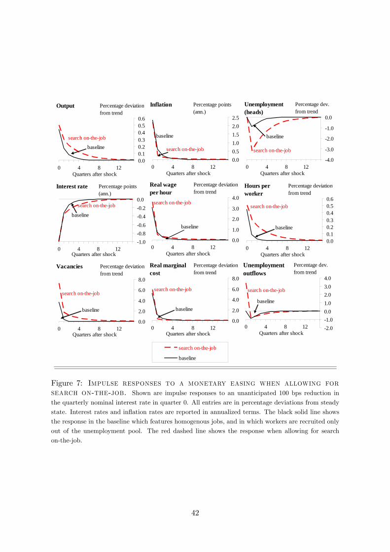
0.00.10.20.30.40.50.6



search onthejob

baseline

Output

0.00.51.01.52.02.5



search onthejob

baseline

Inflation

4.0

3.0

2.0

1.0

0.0



search onthejob

baseline

Unemployment(heads)

1.00.80.60.40.20.0

0 4 8 12


search onthejob

baseline

Interest rate


0.00.10.20.30.40.50.6



search onthejob

baseline

Hours perworker

0.0

1.0

2.0

3.0

4.0



search onthejob

baseline

Real wageper hour

0.0

2.0

4.0

6.0

8.0



search onthejob

baseline

Vacancies

0.0

2.0

4.0

6.0

8.0



search onthejob

baseline

Real marginalcost

2.01.00.01.02.03.04.0



search onthejob

baseline

Unemploymentoutflows

search onthejob

baseline

Figure 7: Impulse responses to a monetary easing when allowing forsearch on-the-job. Shown are impulse responses to an unanticipated 100 bps reduction in

the quarterly nominal interest rate in quarter 0. All entries are in percentage deviations from steady

state. Interest rates and in�ation rates are reported in annualized terms. The black solid line shows

the response in the baseline which features homogenous jobs, and in which workers are recruited only

out of the unemployment pool. The red dashed line shows the response when allowing for search

on-the-job.

42

10 Endogenous job destruction

So far we have treated job separation as an exogenous process occurring at a constant

rate of 6% per quarter. In this we follow much of the literature on frictional labor

markets, which assumes exogenous separation for several reasons: it makes the model

easier to solve; it makes the model easier to calibrate; and it implies a robust negative

correlation between unemployment and vacancies, whereas the Beveridge curve often

disappears in models that endogenize separation.

However, it is disturbing to represent such an important economic decision by an ex-

ogenous constant, so in this section we incorporate an endogenous component into the

separation process. The most obvious motive for endogenizing separation is that the

separation rate rises in recessions (in spite of recent US evidence from Shimer (2005B)

and Hall (2005B) that this countercyclicality is less pronounced than was previously

believed). Sources of evidence for countercyclical separation in Europe include Burda

and Wyplosz (1994); Garibaldi (1998), who shows a negative correlation between job

creation and destruction; and Fredriksen (2003) and D�Addio and Rosholm (2005), who

�nd a negative e¤ect of GDP growth on individual separation rates. Moreover, endog-

enizing separation imposes an additional �rst-order condition related to the separation

margin and thus further restricts the model�s predicted dynamics. It may also help

provide some of the missing variability in unemployment, as Costain and Jansen (2006)

and Mortensen and Nagypal (2007) point out, especially if endogenous separation ap-

plies to newly formed jobs as well as to continuing jobs.31 When endogenous separation

is derived from idiosyncratic productivity shocks, it may also have interesting implica-

tions for productivity and wage dynamics, since it will give rise to a "cleansing e¤ect"

as low productivity matches are destroyed countercyclically.

As in Mortensen and Pissarides (1994), we endogenize separation by assuming that

each match has an idiosyncratic productivity component which is uncorrelated with

aggregate productivity. Thus, the income produced by a match is given by xtzit"ath�it,

where zit is the match-speci�c productivity component and the rest of the notation

follows that in Section 2.32 We will assume zit is normally distributed with distribution

F , which has mean 1 and standard deviation �z. This distribution will allow us to nest

the exogenous search model as a special case of our endogenous search model associated

with �z �! 0.33 We will call the reservation productivity at which separation occurs

31Mortensen and Nagypal (2007) also discuss (exogenous) �uctuations in the job destruction rateas a possible driving force for unemployment �uctuations.32Assuming the idiosyncratic and aggregate productivity components zit and "at enter multiplica-

tively implies that they enter additively in logs, as in the calibration exercise in Sec. 5 of Mortensenand Pissarides (1994).33We will choose parameters such that continuation is optimal for z = 1, implying a reservation

43

zt.

Following den Haan, Ramey, and Watson (2000), we assume zit is iid. That is, zit is

uncorrelated with the aggregate shock xt, it is uncorrelated across individual matches

i, and most importantly it is uncorrelated over time. This matters because it simpli�es

the state space of the model: the equilibrium distribution of productivity is just a

truncated version of the underlying exogenous distribution F . If instead zit were cor-

related over time, high productivity matches would be more likely to survive than low

productivity matches, and we would have to keep track of the endogenous evolution

of the productivity distribution over time. This would require heterogeneous agent

solution methods going far beyond the linear methodology employed elsewhere in the

paper.

For continuity with the setup elsewhere in the paper, we still include an exogenous sep-

aration component: at the end of each period, existing matches separate for exogenous

reasons with probability �x. Allowing for productivity shocks with distribution F in

all periods, and reservation productivity zt, the employment dynamics are:

nt = (1� F (zt)) [(1� �x)nt�1 +mt�1] . (54)

The fraction of jobs surviving between periods t � 1 and t is therefore 1 � �t �(1� F (zt)) (1 � �x). The total number of worker-�rm pairs that meet at the end

of t � 1 is mt�1 = �m v#t�1 u1�#t�1 , where ut�1 = 1 � nt�1 but the number that actually

enter into production at the start of t is only (1� F (zt))mt�1.

The rest of the model has the structure spelled out in Sections 2-3. In particular, we as-

sume e¢ cient bargaining, as in Sec. 3.1, which now implies that both wages and hours

will depend on the match-speci�c productivity shock zit. Thus in the analogue to equa-

tion (17), a matched �rm�s value function is a function of the shock, Jt (zit), and its �ow

of revenues is xtzit"atht(zit)��wt(zit)ht(zit). A matched worker�s value functionWt (zit)

also depends on the shock; the worker�s �ow payo¤s are wt(zit)ht(zit)��1t �1+�

ht(zit)1+�.

On the right-hand side of all the Bellman equations there will therefore be expectations

of future values with respect to zit+1.

E¢ cient bargaining over hours gives a �rst-order condition which is equivalent to (26),

except that it also takes into account the idiosyncratic productivity shock:

ht (z) = (�xt"at�t=�)

11+�� z

11+�� Htz

11+�� (55)

productivity strictly less than one. In the limit as �z �! 0, the fraction separating endogenouslygoes to zero and the mean of z for continuing matches goes to one. Therefore in this limit theadditional �rst-order condition serves only to de�ne the separation threshold, which has no e¤ect onthe remaining equations of the model.

44

Thus hours are proportional to z1

1+�� with the time-varying factor of proportionality

Ht, which will help us aggregate hours and wages. As in Sec. 3.2, the �rst-order

conditions from e¢ cient bargaining can be manipulated to obtain a simpli�ed wage

equation like (32):

wt (z)ht (z) = ��t + (1� �) b+

�� +

� (1� �)

1 + �

�xtzit"

atht(zit)

�

If we make the substitution

ctnt= "at

Z 1

zt

zht (z) dF (z)

then the expected labor income of an employed worker simpli�es to

(1� F (zt))�1Z 1

zt

wt (z)ht (z) dF (z) = ��t+(1� �) b+

�� +

� (1� �)

1 + �

�xtct

(1� F (zt))nt

This substitution allows us to eliminate all integrals over z from the rest of the equi-

librium conditions. In particular, the job creation Euler equation analogous to (30)

becomes

�

qt= Et

(��t+1�t

"(1��)(1+��)

1+�xt+1ct+1nt+1

��1� F

�zt+1

��(��t+1 + (1� �) b) +

�1� �t+1

��qt+1

#)(56)

The reservation productivity zt satis�es the job destruction equation Jt (zt) = 0. Elim-

inating the wage and expected future values from the Bellman equation for J , the job

destruction equation can be written as

(1� �) (1 + �� )

1 + �xt"

atH

�t z

1+�1+��t � ��t � (1� �) b+ (1� �x)

�

qt= 0 (57)

Calibrating this version of the model requires us to determine what fraction of sepa-

rations are endogenous. Davis and Haltiwanger (1995) roughly calculated the fraction

of endogenous separations in US data by comparing �rm-level job destruction (which

they argue should re�ect changes in �rms�labor demand, and therefore map into the

model�s endogenous component) with total worker separation �ows (which are larger,

and should include worker-initiated changes in employment status which they map

into the model�s exogenous component). They �nd that the endogenous component is

roughly 40% of the total, which is the number we will use here. Then for any standard

deviation �z of the idiosyncratic shock, we can calculate z = F�1 (0:4 � 0:06), assuming6% total separation �ows as before, and from z we can calculate all the integrals over

45

z that appear in the equations.

Next, we can back out the other parameters as before: the coe¢ cient �m can be deduced

from observed job �ows; � can be chosen so that the hours bargaining condition (55) is

satis�ed; � is then chosen for consistency with the job creation equation (56). Finally,

we can choose the unemployment income b so that the job destruction equation (57)

holds. This makes the replacement ratio endogenous, so this calibration strategy will

not automatically generate the same replacement rate used in previous sections of the

paper. Therefore, we report a comparison between the endogenous search model and

a simulation of the exogenous search model under the replacement ratio derived from

the endogenous search calculation.

When we calibrate the model for endogenous search, assuming the standard devia-

tion of the idiosyncratic shock is �z = 0:1, we obtain a replacement rate of 84.18%.

Therefore Figure 8 compares these endogenous search results to the exogenous search

model under a replacement rate of 84.18%. With endogenous search, a one-standard

deviation decrease in interest rates causes the separation rate to fall by 15%. Thus,

unemployment reacts immediately to a monetary shock, whereas it exhibits a one pe-

riod lag in the case of exogenous search, and overall this leads to greater variation in

unemployment over time in the case of endogenous search. On the other hand, the

availability of the job destruction margin relaxes the vacancy margin so much that it

goes in the wrong direction: a decrease in interest rates causes vacancies to fall in the

endogenous search model. Also, the availability of the job destruction margin permits

substitution away from the hours margin, so hours increase less than in the exogenous

search case. With less need to increase hours and vacancies, the rise in wages is two

orders of magnitude smaller than it is under exogenous search, and therefore real mar-

ginal cost and in�ation are less volatile too. Higher unemployment volatility together

with lower in�ation volatility are both improvements in the model�s �t to the data, but

the fact that vacancies now go the wrong way relative to unemployment is a serious

problem for this version of the model.

This simulation was based on an arbitrary value of the standard deviation of the idio-

syncratic shock (�z = 0:1). To better determine �z, it would be natural to search for

a value of �z that yields the same replacement ratio used in the baseline model. Inter-

estingly, though, a search over �z reveals regions of qualitatively di¤erent behavior. A

small increase in �z decreases the replacement ratio, bringing it closer to the 65% value

in the baseline model, without qualitative changes in the impulse response functions.

But as we raise �z to 0.4, we come to a region in which equilibrium is indeterminate

(we will not attempt to characterize the model�s behavior in this region). A further

increase, to �z = 0:5, again results in a determinate equilibrium, but one which behaves

46

very di¤erently, as illustrated in Figure 9. In this case, a monetary stimulus causes

labor to increase along all margins: separation falls, while vacancies and hours rise.

We again plot the endogenous search impulse responses together with those of the

exogenous search model under the same replacement ratio. However, this is hard to

see from the graphs, because the impulse responses from endogenous and exogenous

search lie almost directly on top of each other. The reason is that the variation driven by

vacancies is far more signi�cant than that caused by changes in separation rates in this

parameterization. Moreover, since the parameters of the exogenous and endogenous

search cases have been chosen to give the same steady state unemployment rate and

replacement ratio, they have the same surplus in steady state, so that productivity

shocks cause nearly identical variation in vacancies in both cases.

A similar �nding has been reported by Mortensen and Nagypal (2007). They show

observational equivalence of appropriately parameterized endogenous and exogenous

search models with respect to certain statistics (such as the relation between the

volatility of tightness and that of aggregate productivity shocks). While their model

has �exible prices instead of the New Keynesian features considered here, it assumes

a very similar labor market structure, so the intuition for the result is similar: if we

parameterize the steady states of the exogenous and endogenous search models so that

the unemployment rate and replacement ratio are the same, then they will have the

same surplus, and therefore similar hiring incentives.

47

0.0

0.2

0.4

0.6

0.8



endogenous separation

exogenous separation

Output

0.0

0.5

1.0

1.5

2.0




exogenousseparation

Inflation

4.0

3.0

2.0

1.0

0.0





Unemployment(heads)

1.00.80.60.40.20.0

0 4 8 12



exogenousseparation

Interest rate


0.0

0.2

0.4

0.6

0.8




exogenousseparation

Hours perworker

0.01.02.03.04.05.06.0



endogenousseparation

exogenousseparation

Real wageper hour

5.00.05.010.015.020.0





Vacancies

0.02.04.06.08.010.0




exogenousseparation

Real marginalcost

4.02.00.02.04.06.08.0






endogenous separationexogenous separation (baseline)

Figure 8: Impulse responses to a monetary easing, model with endogenousseparation vs. model with exogenous separation. Shown are impulse responses toan unanticipated 100 bps reduction in the quarterly nominal interest rate in quarter 0. All entries are

in percentage deviations from steady state. Interest rates and in�ation rates are reported in annualized

terms. The black solid line refers to the response in a model, which features only exogenous separation

between �rms and workers. Apart from slight di¤erences in the calibration (described in the main

text body) this resembles the baseline model. The red dashed line marks the responses when allowing

for endogenous separation. Shown is the case with a low standard deviation of the idiosyncratic

technology shock, �z = 0:1:

48

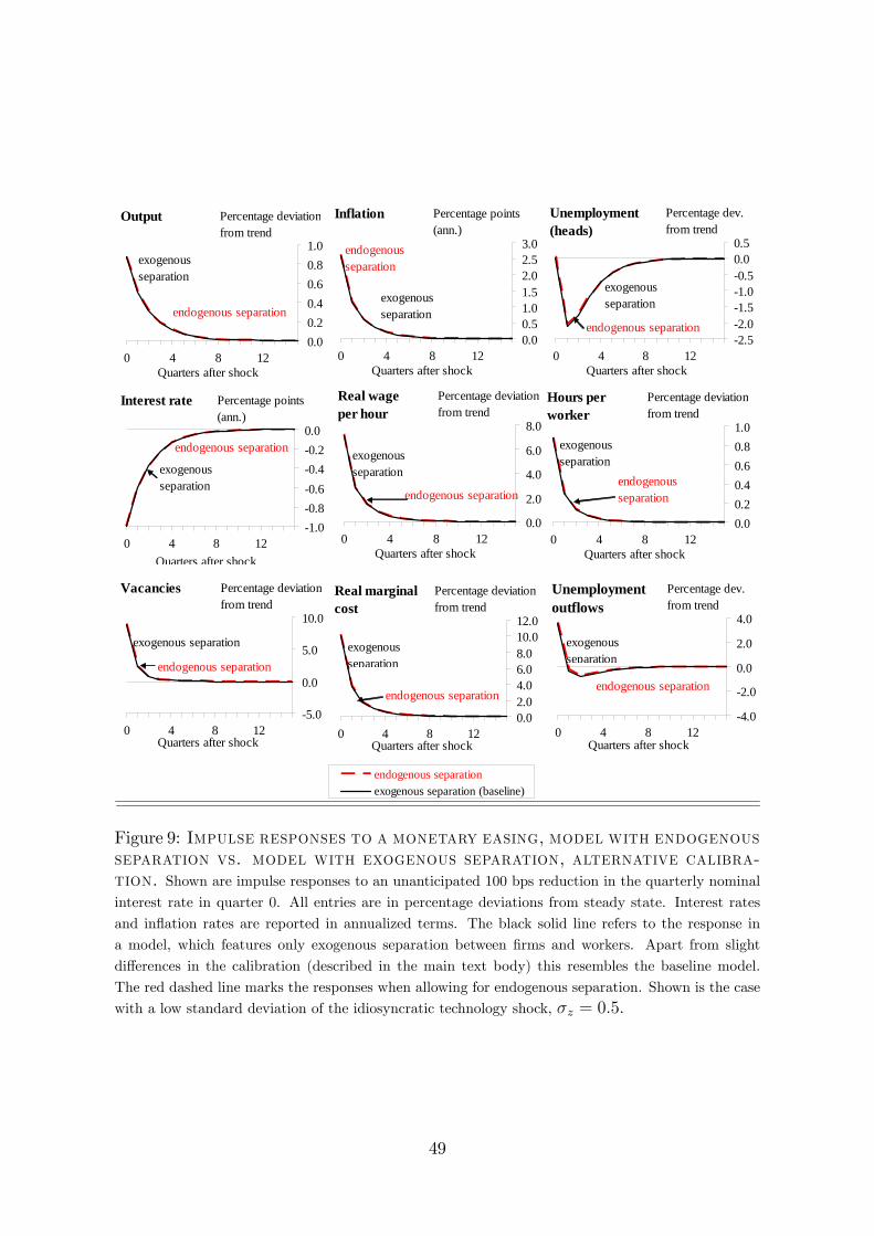
0.00.20.40.60.81.0




exogenousseparation

Output

0.00.51.01.52.02.53.0




exogenousseparation

Inflation

2.52.01.51.00.50.00.5




exogenousseparation

Unemployment(heads)

1.00.80.60.40.20.0

0 4 8 12



exogenousseparation

Interest rate


0.00.20.40.60.81.0




exogenousseparation

Hours perworker

0.0

2.0

4.0

6.0

8.0




exogenousseparation

Real wageper hour

5.0

0.0

5.0

10.0





Vacancies

0.02.04.06.08.010.012.0




exogenousseparation

Real marginalcost

4.0

2.0

0.0

2.0

4.0




exogenousseparation


endogenous separationexogenous separation (baseline)

Figure 9: Impulse responses to a monetary easing, model with endogenousseparation vs. model with exogenous separation, alternative calibra-tion. Shown are impulse responses to an unanticipated 100 bps reduction in the quarterly nominalinterest rate in quarter 0. All entries are in percentage deviations from steady state. Interest rates

and in�ation rates are reported in annualized terms. The black solid line refers to the response in

a model, which features only exogenous separation between �rms and workers. Apart from slight

di¤erences in the calibration (described in the main text body) this resembles the baseline model.

The red dashed line marks the responses when allowing for endogenous separation. Shown is the case

with a low standard deviation of the idiosyncratic technology shock, �z = 0:5:

49

11 Conclusions

In this paper, we have assessed the ability of a host of New Keynesian models with

alternative labour market speci�cations to explain in�ation dynamics. We �rst used

a standard New Keynesian model with search and matching to show that such models

typically generate a response of in�ation to nominal shocks that is much too large

relative to the data. We then considered some alternative speci�cations.

We �rst considered the addition of wage rigidity. Under e¢ cient bargaining, wage

stickiness in existing jobs has no e¤ect since average wages are non-allocative in this

set up. But, if the nominal wage of newly-created jobs is sticky, then there will be

an e¤ect. In this case, the existing wage rate will a¤ect real marginal cost, since

the wage paid to new hires a¤ects hiring incentives. With real marginal cost sticky,

in�ation will respond less to nominal shocks. Perhaps more interestingly, we found

that nominal wage rigidity can have a further role in a monetary model. Combined

with a �right-to-manage�assumption for the determination of hours (which implies a

direct channel from wages to in�ation), staggered wages at the level of the match will

help to smooth the reaction of the aggregate wage resulting in a smaller response to

shocks of marginal cost and in�ation. When we then combined this nominal rigidity

with the real rigidity of �rm-speci�c labour, we found that prices respond less to shocks

the more any �rm�s marginal costs respond to a change of the �rm�s price. Hence, the

response of in�ation to nominal shocks is reduced if the marginal disutility of work is

increasing in hours worked and/or there are decreasing returns to labour; both these

conditions hold in our calibrated model.

We then looked at variants of the model in which hiring costs were either proportional

to the hiring rate or sunk (i.e., unrelated to the number of vacancies opened). We

found that neither of these modi�cations a¤ected the response of in�ation to nominal

shocks, which was still too large. We then considered two other margins along which

adjustment can occur in the labour market: on-the-job search and endogenous job

destruction. We found that both features could help reduce the response of in�ation

to shocks, though our results based on endogenous job destruction depended critically

on the calibration of the model.

In summary, we found that a model with sticky nominal wages when combined with

right-to-manage bargaining was best able to capture unemployment volatility and the

response of in�ation to nominal shock. In that setup it was largely irrelevant whether

wage stickiness a¤ected only existing matches or also new matches. [More nuancedhere?] The current paper therefore �nds that if the labour market were to matter forin�ation dynamics, it would most likely be the case for the above reasons. We have

not been able to make a clear case, however, that the labour market would necessarily

50

matter for in�ation dynamics. The reason is the lack of micro-evidence to discern

di¤erent modeling strategies.

For future work, it would therefore be interesting to put the mechanisms that we have

explored to a test from micro-economic perspective. Work on wage stickiness for new

hires that has recently been conducted, e.g., by Haefke et al. (2007) is a �rst step in that

direction. Micro-evidence on bargaining and contractual arrangements regarding state

contingency of the wage, overtime payments and premia, overtime accounts and non-

wage components of compensation would be a valuable further step towards discerning

the di¤erent labour market setups.

References

[1] Akerlof, G., A. Rose and J. Yellen (1988), �Job switching and job satis-faction in the US labor market�, Brookings Papers on Economic Activity, Vol. 2,

pages 495-594.

[2] Alvarez, L., E. Dhyne, M. Hoeberichts, C. Kwapil, H. Le Bihan, P.Lünnemann, F. Martins, R. Sabbatini, H. Stahl, P. Vermeulen, and J.Vilmunen (2006), �Sticky prices in the euro area: a summary of new microevidence�, Journal of the European Economic Association, 4, 575�584.

[3] Angeloni, I., A. Kashyap, B. Mojon and D. Terlizzese (2003), �The outputcomposition puzzle: a di¤erence in the monetary transmission mechanism in the

euro area and United States�, Journal of Money, Credit, and Banking, Vol. 35,

No. 6 , 1265�1306.

[4] Ball, L., and D. Romer (1990), �Real rigidities and the non-neutrality ofmoney�, Review of Economic Studies, 57(2), 183-203.

[5] Bernanke, B., J. Boivin and P. Eliasz (2005), �Measuring the e¤ects of

monetary policy: a factor-augmented vector autoregressive (FAVAR) approach�,

Quarterly Journal of Economics, 120(1), 387-422.

[6] Blanchard, O., and J. Gali (2006), �A New Keynesian model with unemploy-ment�, National Bank of Belgium Working Paper No. 92.

[7] Blanchard, O., and J. Gali (2007), �Real wage rigidities and the New Key-nesian model�, Journal of Money, Credit and Banking, Vol. 39(1), 35-65.

51

[8] Bodart, V., G. de Walque, O. Pierrard, H. Sneessens, and R. Wouters(2006), �Nominal wage rigidities in a New Keynesian model with frictional unem-ployment�, IZA Discussion Paper No. 2528.

[9] Bodart, V., O. Pierrard and H. Sneessens (2005), �Calvo wages in a searchunemployment model�, DNB Working Paper No. 68.

[10] Burda, M., and C. Wyplosz (1994), �Gross worker and job �ows in Europe�European Economic Review, 38(6), 1287�1315.

[11] Christiano, L., M. Eichenbaum, and C. Evans (2005), �Nominal rigidi-ties and the dynamic e¤ects of a shock to monetary policy�, Journal of Political

Economy, Vol. 113, pages 1-45.

[12] Christo¤el, K., K. Kuester and T. Linzert (2008), �The Role of labourMarkets for Euro Area Monetary Policy�, mimeo. European Central Bank.

[13] Christo¤el, K., and T. Linzert (2005), �The role of real wage rigidity andlabour markets frictions for unemployment and in�ation dynamics�, ECB Working

paper No. 556.

[14] Christo¤el, K. and K. Kuester (2008), �Resuscitating the wage channelin models with unemployment �uctuations�, forthcoming Journal of Monetary

Economics.

[15] Contini, B., and R. Revelli (1997), �Gross �ows vs. net �ows in the labormarket: What is there to be learned?�, Labour Economics, Vol. 4, pages 245-63.

[16] den Haan, W., G. Ramey, and J. Watson (2000), �Job destruction andpropagation of shocks�, American Economic Review, Vol. 90(3), pages 482-498.

[17] Druant, M., S. Fabiani, I. Hernando, C. Kwapil, B. Landau, C.Loupias, F. Martins, T.Y. Matha, R. Sabbatini, H. Stahl and A.C.J.Stokman (2006), �The pricing behaviour of �rms in the Euro Area: new surveyevidence�, International Journal of Central Banking, Vol. 2(3), pages 3-47.

[18] du Caju, P., E. Gautier, D. Momferatou, and M. Ward-Warmedinger(2008), �Institutional features of wage bargaining in 22 EU countries, the US andJapan�, mimeo. European Central Bank, Frankfurt am Main.

[19] Evers, M., R. A. D. Mooij, and D. J. V. Vuuren (2005):, �What explainsthe variation in estimates of labour supply elasticities?�, CESifo Working Paper

No. 1633, CESifo, Munich.

52

[20] Faia, E. (2008), �Optimal monetary policy rules with labour market frictions�,forthcoming Journal of Economics Dynamics and Control.

[21] Fujita, S., and G. Ramey (2005), �The dynamic beveridge curve�, FederalReserve Bank of Philadelphia Working Paper No. 05-22.

[22] Gali, J., M. Gertler and D. Lopez-Salido (2001), �European in�ationdynamics�, European Economic Review, Vol. 45, pages 1,237-70.

[23] Gertler, M. and A. Trigari (2006), �Unemployment �uctuations with stag-gered Nash wage bargaining�, NBER Working Paper No. 12498..

[24] Gomes, P. (2007), �Labour market �ows in the United Kingdom�, Bank of Eng-land, mimeo.

[25] Haefke, C., M. Sonntag, and T. van Rens (2007), �Wage rigidity and jobCreation �, mimeo. Universitat Pompeu Fabra.

[26] Hall, R. E. (2005), �Employment �uctuations with equilibrium wage stickiness�,American Economic Review, Vol. 95(1), pages 50-65.

[27] Hall, R.E. and P.R. Milgrom (2007), �The limited in�uence of unemploy-ment on the wage bargain�, Stanford University, mimeo.

[28] Hobijn, B., and A. Sahin (2007), �Job-Finding and Separation Rates in theOECD�, Sta¤ Report no. 298, Federal Reserve Bank of New York.

[29] Krause, M., and T. Lubik (2006), �The cyclical upgrading of labour andon-the-job search�, Labour Economics, Vol. 13, pages 459-77.

[30] Krause, M., and T. Lubik (2007), �The (ir)relevance of real wage rigidity inthe New Keynesian model with search frictions�, Journal of Monetary Economics,

Vol. 54 (3), pages 706-27.

[31] Kuester, K. (2007), �Real price and wage rigidities in a model with matchingfrictions�, European Central Bank Working Paper No. 720.

[32] McCallum, A., and F. Smets (2008), �Real wages and monetary policy trans-mission in the euro area�, mimeo. European Central Bank.

[33] Merz, M. (1995), �Search in the labour market and the real business cycle�,Journal of Monetary Economics, Vol. 36, pages 269-300.

53

[34] Millard, S. and C. Ellis (2007), �Price setting and in�ation dynamics: thestate of the art�, Bank of England, mimeo.

[35] Mojon, B., and G. Peersman (2003). �A VAR description of the e¤ects of

monetary policy in the individual countries of the euro area�, In: Monetary Policy

Transmission in the Euro Area, edited by I. Angeloni, A. Kashyap, and B. Mojon,

pp. 56�74. Cambridge, UK: Cambridge University Press.

[36] Mortensen, D., and C. Pissarides (1994), �Job creation and job destructionin the theory of unemployment�, Review of Economic Studies, Vol. 61, No.3, pages

397-415.

[37] Mortensen, D., and C. Pissarides (1999), �Job reallocation, employment�uctuations and unemployment�, in Handbook of Macroeconomics, ed. by J. Tay-

lor and M. Woodford, Vol. 1, chap. 18, pages 1171-12228. Amsterdam: North-

Holland.

[38] Normandin, M. (2006), �The e¤ects of monetary-policy shocks on real wages:a multi-country investigation�, Cahiers de recherche 06-04, Institut d�économie

appliquée HEC Montréal.

[39] Okun, A. M. (1973), �Upward mobility in a high-pressure economy�, BrookingsPapers on Economic Activity, Vol. 1, pages 207-52.

[40] Peersman, G., and F. Smets (2003), �The monetary transmission mecha-

nism in the euro area: more evidence from VAR analysis�, In: Monetary Policy

Transmission in the Euro Area, edited by I. Angeloni, A. Kashyap, and B. Mojon,

pp. 36�55. Cambridge, UK: Cambridge University Press.

[41] Peersman, G., and R. Straub (2007), �Putting the New Keynesian model toa test�, mimeo. European Central Bank.

[42] Petrongolo, B., and C. A. Pissarides (2001), �Looking into the black box:a survey of the matching function�, Journal of Economic Literature, 2001(2), 390�

431.

[43] Pissarides, C. A. (2007), �The unemployment volatility puzzle: is wage sticki-ness the answer?�, mimeo. London School of Economics.

[44] Ravenna, F., and C. Walsh (2007), �Vacancies, unemployment and the

Phillips curve�, mimeo, University of California at Santa Cruz.

54

[45] Shimer, R. (2005), �The cyclical behaviour of equilibrium unemployment and

vacancies�, American Economic Review, Vol. 95, pages 25-49.

[46] Smets, F., and R. Wouters (2003): �An estimated stochastic dynamic generalequilibrium model of the euro area�, Journal of the European Economic Associa-

tion, 1(5), 1123-75.

[47] Sveen, T., and L. Weinke (2007), �In�ation dynamics and labour marketdynamics revisited �, Kiel Working Papers No. 1368, Kiel Institute for the World

Economy.

[48] Tang, J.-H. (2006), �Optimal monetary policy in a New Keynesian model withjob search�, mimeo. National Tsing-Hua University, Taiwan.

[49] Thomas, C. (2008), �Search frictions, real rigidities and in�ation dynamics �,mimeo. Banco de España, February 2008.

[50] Trigari, A. (2005), �Equilibrium unemployment, job �ows, and in�ation dy-

namics�, Bocconi University Working Paper No. 268.

[51] Trigari,A. (2006), �The role of search frictions and bargaining for in�ationdynamics�, Bocconi University Working Paper No. 268.

[52] van Zandweghe, W. (2006), �On-the-job search, sticky prices and persistence�,Tepper School of Business, mimeo.

[53] Walsh, C. (2005), �labour market search, sticky prices, and interest rate policies,�Review of Economic Dynamics, 8, 829-849.

[54] Woodford, M. (2003), �Interest and prices�, Princeton University Press: Prince-ton.

[55] Yashiv, E. (2006), �Evaluating the performance of the search and matchingmodel�, European Economic Review, 50(May), 909-936.

[56] Zanetti, F. (2007), �Labour market institutions and aggregate �uctuations in asearch and matching model�, Bank of England Working Paper No. 333.

12 Appendix A: further evidence on monetary trans-

mission in the euro area

In the paper, we benchmarked the di¤erent approaches to modelling the labor market

against �ve stylized facts about the transmission of monetary policy in the euro area.

55

This section presents the background evidence from which we deduced these stylized

facts.34

Figure 1 prints the impulse responses of euro area aggregates to a 100bps monetary

shock (an easing) in McCallum and Smets (2008),35 who estimate a Factor-Augmented

VAR following the methodology of Bernanke et al. (2005). Also shown are the bound-

aries of bootstrapped 90% con�dence intervals. According to this evidence, a monetary

2.01.00.01.02.03.0

0 4 8 12


Percentagedeviationfrom trend

Output

1.0

0.5

0.0

0.5

0 4 8 12


Quarteronquarter,percentage points (ann.)

Inflation

15.010.05.00.05.010.0

0 4 8 12


Percentagedeviation fromtrend

Unemployment

1.51.00.50.00.51.0

0 4 8 12



InterestRate

0.00.20.40.60.8


Percentagedeviationfrom trend


Figure 10: Impulse responses to an unanticipated monetary shock in theeuro area, source: McCallum and Smets (2008). Depicted are responses to a

100 bps monetary easing (annualized nominal rates). Charts refer to the euro area. The sample

is 1987Q1 to 2005Q4. Top row (from left to right): response of real GDP (in percentage deviation

from trend), quarter-on-quarter GDP in�ation (in annualized percentage points), unemployment (in

percentage deviation from trend). Note: shown is the response of log unemployment (heads), log(ut).

Bottom row: response of nominal interest rate (in annualized percentage points) and the real wage

per employee (in percentage deviation from trend). Source: McCallum, Smets (2008), reprinted with

the author�s permission.

easing stimulates the economy. At its peak, output has risen by about 0.8% above

steady state. In�ation increases, too, but in a muted manner. The peak increase in

quarter-on-quarter GDP in�ation is about 25bps (in annualized terms). As a conse-

34A number of studies have examined the response of real and nominal variables in the euro areato a monetary shock using alternative identi�cation mechanisms. For early evidence on the euro areaas a whole, see e.g. Peersman and Smets (2003) and Angeloni et al. (2003). More recent papers areMcCallum and Smets (2008) and Peersman and Straub (2007). For evidence country by country seee.g. Mojon and Peersman (2003) and Normandin (2006).35Their data comprise quarterly euro area aggregates and a number of euro-area country-speci�c

series from 1987Q1 to 2005Q4, as well as foreign series.

56

quence of higher demand, the number unemployed people, i.e., unemployment, falls

by 3%.36 The increase in economic activity also translates into an increase in the real

wage per employee. That increase is about half the size of the increase in output, but

is very persistent.

Complementing this evidence, Figure 11 reports our own estimates of the monetary

transmission in the euro area. The sample starts in 1987Q1 as in McCallum and Smets

(2008), and runs through 2006Q4. We estimated a standard VAR(4) in the variables

shown in the graphs, and identi�ed the monetary shock through the oft-used recursive

ordering scheme. For details see the notes to Figure 11. According to these estimates,

an unanticipated monetary easing induces a longer-lived deviation of nominal rates

from the baseline than in McCallum and Smets (2008) and, as a result, most responses

are more persistent. With regard to amplitudes, the evidence is robust, however. A

monetary easing by 100bps causes a notable increase in output of about 0.8% at its

peak, and an increase in real wages per employee of about half that size (which is,

again, very persistent). Unemployment, according to our estimates, falls by 6% below

steady state.37 At the same time, the increase in in�ation remains contained, with

(GDP) in�ation remaining below 0.4 percentage points in annualized terms.

In the above estimation, we resort to the same proxy for hours worked in the euro

area as used by Christo¤el et al. (2008).38 When using this series to infer hourly wage

rates and hours worked per employee, the results suggest that changes at the extensive

margin are more relevant for labor adjustment than hours worked per employee. Hours

worked per employee react very little throughout the period (and if anything, they fall),

while the number of employees is more responsive. See the �rst two panels of Figure

12. As a result, the increase in wages per employee depicted in Figure 11 is mainly

attributed to a slow but persistent increase in hourly wages instead of an increase in

hours per worker, see Figure 12. Due to the limitations of the euro area data with

respect to hours worked or hourly wages, however, the responses in Figure 12 �while

indicative �should be taken with a relatively large grain of salt.

Table 3, �nally, summarizes the impulse responses reported above, and augments these

by evidence of three further studies. Angeloni et al. (2003) report impulse responses

36This refers to unemployment, not to unemployment rates in percentage points. The depictedfall in unemployment corresponds to a fall in unemployment rates of about .27 percentage points.Unemployment is calculated in a model-consistent from the response in employment, which McCallumand Smets report, by assuming that the labor force does not react to a monetary easing, and thataverage unemployment rates are 9%37This translates into a reduction in unemployment rates of about .54 percentage points.38Unfortunately, harmonized quarterly series for hours worked do not exist for the euro area. The

proxy uses the quarterly real GDP series for the euro area to interpolate annual EU-Klems data ontotal hours worked in the euro area.

57

1.00.50.00.51.01.52.0

0 4 8 12



Output

15.0

10.0

5.0

0.0

5.0

0 4 8 12



Unemployment

0.5

0.0

0.5

1.0

0 4 8 12



Real wageper employee

0.5

0.00.5

1.01.5

2.0



Total hoursworked

2.0

1.0

0.0

1.0

2.0

0 4 8 12


Percentagepoints (ann)

Interest rate

1.0

0.5

0.0

0.5

1.0

0 4 8 12


Quarteronquarter,percentage points(ann.)

Inflationrate

Figure 11: Impulse responses to an unanticipated monetary shock �ownestimates. Underlying the results is a VAR(4) estimated on above data (taken from the AWM data

set except four hours worked, which is taken from Christo¤el et al., 2008). The sample is 1987Q1 to

2006Q4, identi�cation relies on the usual Cholesky decomposition. The data was de-trended variable

by variable prior to running the VAR. For real variables, we allow for a trend, and a break in the

trend plus a level shift in 1991Q1 so as to accommodate German reuni�cation. In�ation and mominal

interest rates were regressed on a linear trend, which breaks after 1998Q4 in order to account for the

disin�ation in the euro area prior to the introduction of the common currency, and the constancy of

the in�ation objective thereafter. Dotted lines mark asymptotic 90% con�dence intervals (5% and

95% bounds).

for the euro area based on various identi�cation schemes for the monetary shock in a

VAR. So do Peersman and Smets (2003). The Table, in addition, collects evidence of

a recent study by Peersman and Straub (2007) who identify a monetary shock (and

other shocks) based on sign restrictions, which were derived from a prototypical New

Keynesian model. The Table summarizes the maximum amplitudes of the variables

following the monetary shock. Most of the studies imply that after the initial shock,

nominal rates fall somewhat further before being tightened. In order harmonize the

studies, all responses have been normalized by the maximum easing of the nominal

interest rate that these studies report.

58

0.5

0.0

0.5

1.0

0 4 8 12



Real wageper hour

Quarters after shock0.6

0.4

0.2

0.0

0.2

0.4

0 4 8 12



Hours perworker

0.50.00.51.01.52.02.5



Employment(heads)

Figure 12: Impulse responses of hours and wages to a monetary shock �own estimates. Shown are the responses of employment, hours per employee and the real wagerate. The VAR is the same as in Figure 11, except that the a measure of hours per worker and of the

real hour wage rate replaces the measures for total hours worked and the real wage per employee.

Out-put

In�. Un-empl.

Empl. Realwagesperempl.

Realwageperhour

Totalhourswor-ked

Hoursperempl.

McCallum,Smets (1) 0.7 0.2 -2.9 0.3 0.4 � � �Own VAR (2) 0.6 0.3 -4.5 0.4 0.3 0.4 0.9 0.04

Peersman,Straub (3) 0.3 0.2 -2.8 0.3 0.3 0.3 0.3 0

Angeloni et al. (4) 0.5 0.2 -3.3 0.3 � � � �Peersman,Smets (5) 0.5 0.2 -3.3 0.3 � � � �

Table 3: Peak responses to a monetary easing in the literature. Mostof the studies imply that after the initial easing, nominal rates fall somewhat further before theytighten. In order harmonize the studies, all responses have been normalized by the maximum easingof the nominal interest rate that these studies report (which in all studies occurs one quarter afterthe shock). Entries in small type refer to numbers that have been deduced indirectly as describedbelow. (1): McCallum and Smets (2008) report the response of employment. The response forunemployment is inferred from the �gure for employment assuming a constant labor force andan average unemployment rate of 9%. (2): Own VAR: hours worked data for the euro area issubject to measurement errors as stated in the main text. (3): Peersman and Straub (2007) onlyreport the response of total hours worked, but state that responses are similar when employmentis used. We thus report the same response of employment as for total hours worked. The responsefor unemployment is inferred as in (1). Similarly, hourly wage rates and hours per employee areinferred from this statement. (4): Peersman, Smets (2003): sample 1980-1998. Entries are basedon their Fig. 2.1 and Fig. 2.8. The response for unemployment is inferred as in note (1). (5):Angeloni et al. (2003) report the response of the unemployment rate (see their Table 6). Theresponse of unemployment reported here is obtained using an unemployment rate of 9%. Figuresfor employment were obtained accordingly. Results for the Angeloni et al. paper are averages overdi¤erent speci�cations for the sample 1980-2001. Only the response of consumer prices is reported.Results were read-o¤ the Figures and Tables in their paper.

59

european summer symposium in international macroeconomics ... · the –rm level between price and...

Documents