eurostat review on ational accounts and …
TRANSCRIPT

EUROSTAT REVIEWON NATIONAL ACCOUNTSAND MACROECONOMIC INDICATORS1/2018


EUROSTAT REVIEWON NATIONAL ACCOUNTS
AND MACROECONOMIC INDICATORS 1/2018

Printed by Imprimerie Centrale in LuxembourgManuscript completed in June 2018
Neither the European Commission nor any person acting on behalf of the Commission is responsible for the use that might be made of the following information.
Luxembourg: Publications Office of the European Union, 2018
© European Union, 2018Reuse is authorised provided the source is acknowledged. The reuse policy of European Commission documents is regulated by Decision 2011/833/EU (OJ L 330, 14.12.2011, p. 39).
For any use or reproduction of photos or other material that is not under the EU copyright, permission must be sought directly from the copyright holders.For more information, please consult: http://ec.europa.eu/eurostat/about/policies/copyright
The information and views set out in this publication are those of the authors and do not necessarily reflect the official opinion of the European Union. Neither the European Union institutions and bodies nor any person acting on their behalf may be held responsible for the use which may be made of the information contained herein.
Theme: Economy and financeCollection: Statistical books
Print ISSN 2443-7832 Cat.: KS-GP-18-001-EN-CPDF ISSN 1977-978X Cat.: KS-GP-18-001-EN-N

Contents
EURONA — Eurostat Review on National Accounts and Macroeconomic Indicators 3
Contents
Editorial 5
R&D capitalisation: where did we go wrong? Mark de Haan and Joseph Haynes 7
How to measure hedonic property price indexes better Mick Silver 35
Mixed-form indices: a study of their properties Bert M. Balk 67
Dynamic pricing as a challenge for consumer price statistics Christian Blaudow and Florian Burg 79
In memoriam: Peter Hill (1929-2017) 95

Aims and scope
EURONA — Eurostat Review on National Accounts and Macroeconomic Indicators4
Aims and scopeEURONA is an open access, peer-reviewed, scholarly journal dedicated to National Accounts and Macroeconomic Indicators. EURONA aims at providing a platform for researchers, scholars, producers and users of macroeconomic statistics to exchange their research findings, thereby facilitating and promoting the advancement of National Accounts and Macroeconomic Indicators.
EURONA publishes empirical and theoretical articles within the scope of National Accounts and Macroeconomic Indicators, as well as articles on important policy uses of these statistics. They may relate to both users’ and producers’ interests, present subjects of general relevance or investigate specific topics.
EURONA is non-partisan and applies the highest standards to its content, by emphasising research integrity, high ethical standards, validity of the findings and cutting edge results. EURONA gives room to all viewpoints.
The articles published in EURONA do not necessarily reflect the views or policies of the European Commission.
Website: http://ec.europa.eu/eurostat/web/national-accounts/publications/eurona
Contact: [email protected]
EditorsPaul Konijn (1), Eurostat
Editorial boardSilke Stapel-Weber, Eurostat
Albert Braakmann, Statistisches Bundesamt
Gerard Eding, Centraal Bureau voor de Statistiek
Rosmundur Gudnason, Statistics Iceland
Robert Inklaar, University of Groningen, the Netherlands
Sanjiv Mahajan, Office for National Statistics
Gabriel Quiros, International Monetary Fund
Philippe Stauffer, Federal Statistical Office
Peter van de Ven, Organisation for Economic Co-operation and Development(1) [email protected]

Editorial
EURONA — Eurostat Review on National Accounts and Macroeconomic Indicators 5
Editorial
Three of the four articles in this issue of EURONA were presented at the meeting of the Ottawa group on price indices in Germany, May 2017. The Ottawa group is one of the so-called ‘city groups’ that work under the auspices of the United Nations Statistical Commission and has been discussing and developing the theory and practice of price indices since 1994.
Mick Silver’s article discusses the measurement of (residential and commercial) property price indices. The main difficulties in measuring property price indices are the infrequency of transactions and the heterogeneity of properties. Hedonic regression methods are recommended in such circumstances and the author discusses the best practices to apply these methods.
Christian Blaudow and Florian Burg discuss the challenges posed to consumer price statistics by the increase in dynamic pricing practices for consumer price indices. Dynamic pricing refers to the frequent and automated adaptation of prices charged for products (mainly sold online) in reaction to, for example, changes in demand or supply. The authors analyse data obtained by web scraping, in other words, the automatic collection of price data on the internet, to examine the extent of such practices.
One session of the 2017 Ottawa group meeting was dedicated to the memory of Peter von der Lippe (1942-2016), who devoted his working life to economic statistics with a special interest for price indices. He was especially passionate about the subject of chain indices, of which he was one of the most vocal opponents. Bert Balk’s commemorative paper deals with ‘mixed-form’ indices, in other words, indices that behave as direct (fixed base) indices in the short run (on a monthly basis) but as chain indices over the long run (on an annual basis).
However, this issue opens with an article from Mark de Haan and Joseph Haynes on an important and topical national accounts issue: the capitalisation of research and development expenditures, specifically in the context of globalisation. The main question is how to decide, in a world of global value chains, at which location a specific intellectual property product (for example, an R&D asset) is used in production. The authors describe and analyse two specific cases of multinational enterprises that clearly demonstrate the challenges and risks for the quality of economic statistics. To mitigate these risks, the authors conclude that enhanced cooperation and data sharing between national statistical institutes is necessary.
Finally, the issue closes by paying tribute to T. Peter Hill (1929-2017), who made numerous contributions to national accounts and price statistics during his career, most notably as the driving force behind the SNA 1993. The obituary, written by his son Robert J. Hill, is reproduced courtesy of the Review of Income and Wealth.
Paul Konijn
Editor of EURONA
Editorial


1 R&D capitalisation: where did we go wrong?MARK DE HAAN, JOSEPH HAYNES (1)
Abstract: this paper is an attempt to contribute to the discussion of research and development (R&D) capitalisation in the system of national accounts. The paper first spells out under which conditions knowledge creation truly leads to fixed assets in the national accounts sense.
As a next step, R&D capitalisation is examined in the context of globalisation. One of the serious problems that multinational enterprise (MNE) groups present for macro-economic measurement is the issue of assigning economic ownership of R&D, and intellectual property (IP) more generally, to the various fractions of a global value chain and therefore to domestic economies. This is an issue for which international guidance is currently incomplete and still under research by national accountants. In this paper the discussion of IP focuses largely on R&D.
By analysing real world companies and their production processes this paper aims to highlight some of the issues with the current recording treatment around IP. This translation of information on the MNE group’s business structure to the national accounts framework will give an indication of real world distortions that national accountants may encounter when measuring the activities of MNE groups on a domestic economy basis.
All the information contained within this paper relating to these MNE groups is taken from previously published publically available sources. There may be deficiencies in the way the characteristics of these MNE group structures are being revealed by these sources. We nevertheless take these available sources as the starting point of this paper with the main purpose of highlighting the complexities of recording these structures in the national accounts.
This paper offers a number of proposals for improvements though definite solutions to the issues are not possible in one paper alone. Perhaps the greatest contribution of this paper is in highlighting clearly the need for openness and data sharing between national statistics institutes (NSIs). Accurate recording of the activities of MNE groups requires cooperation and data sharing at a far greater level than NSIs have previously been willing to do.
JEL codes: E01, F62
Keywords: national accounts, intellectual property, globalisation
(1) National accounts department, Statistics Netherlands.

R&D capitalisation: where did we go wrong?
EURONA — Eurostat Review on National Accounts and Macroeconomic Indicators8
1
1. Introduction
(2) The misplaced conceptual argument in which public R&D is compared with public infrastructure is discussed later on in this paper.
A significant innovation in the latest System of National Accounts (SNA) update (2008 SNA) was the capitalisation of expenditure on research and development (R&D). In the process of the SNA update, Statistics Netherlands produced several papers on this issue (de Haan and van Rooijen-Horsten (2004) and van Rooijen-Horsten et al. (2007)). These papers highlighted several data issues such as: the translation of Frascati Manual (OECD (2015)) based R&D statistics to national accounts data; assessing service lives of R&D assets; and dealing with possible overlaps between R&D and computer software. This kind of guidance was later formalised in the OECD’s Handbook on Deriving Capital Measures of Intellectual Property Products (2009). While the 1993 SNA implementation included the introduction of computer software capitalisation for which the first country results showed a disparity of applied methods and results, the introduction of R&D capitalisation was ‘managed’ in a more careful way. Unfortunately, we cannot conclude that R&D capitalisation in the national accounts has been totally successful.
In the papers produced by Statistics Netherlands, two conceptual concerns were brought to attention:
• R&D in the public domain does not necessarily comply with the general definition of an asset in the SNA sense. Economic ownership of public knowledge cannot be claimed by one particular economic agent;
• Guidance on how to account for R&D flows and stocks inside multinational enterprises (MNEs) is totally lacking.
Supporters of the first proposition (for example, representatives from Statistics Denmark, Statistics Netherlands and the United Kingdom’s Office for National Statistics) ’lost the battle’. Ultimately, it was decided that R&D expenditure, both public and private, should be treated equally as fixed assets in the 2008 SNA. The arguments supporting this choice were pragmatic rather than conceptual. Our impression is still that publicly available knowledge contrasts with the general SNA definition of an economic asset (2). This broad demarcation of R&D assets is also ambiguous and creates implausible outcomes. Therefore, we revisit this issue in the subsequent section of this paper before moving on to the issue of globalisation.
In recent years, a second issue on R&D within MNE groups and globalisation has received increasing attention. For national accountants, one of the key challenges of economic globalisation is explaining how capital services of intellectual property (IP) enter globally organised production chains. Several developments are complicating this globalisation puzzle. Firstly, the international fragmentation of production chains, inside or outside MNE structures, may imply that business functions such as R&D and software development (in other words, product development and design, development of software inputs) are being separated and (spatially) disconnected from the process of physical transformation (the actual manufacturing of the good embedding the IP). Secondly, production chain fragmentation may also enter the stages of physical transformation. Examples of highly fractured and specialised manufacturing webs are those found in the automobile or aircraft industries.

R&D capitalisation: where did we go wrong?
EURONA — Eurostat Review on National Accounts and Macroeconomic Indicators 9
1Nowadays, some manufacturers entirely offshore the physical transformation stages of production; such ‘production arrangers’ are also called factoryless goods producers (FGPs). The issue of FGPs was intensively discussed in the UNECE task force on global production (2015). Questions about their economic classification and the kinds of transaction these companies are generally engaged in were, unfortunately, not brought to a final conclusion. Both issues are closely linked to recording R&D or, more generally, IP flows and stocks.
R&D capitalisation suggests that IP products can be accounted for like any other fixed asset in the national accounts. Our view on globalisation is that this is not the case. This point is picked up in Section 3 of this paper.
An additional complicating factor is that IP, or intangible assets more broadly, may become a vehicle for tax planning. MNE groups may locate their IP and report related IP revenues (in other words, royalties) in low tax jurisdictions and subsequently charge affiliated companies, which report substantive shares of the group’s turnover, for the use of the IP. Such tax planning arrangements may involve a range of special purpose entities (SPEs) located in a variety of countries. A national accountant is usually able to observe only fragments of the tax planning arrangement and is easily misled by the information being obtained at the level of individual SPEs, or other entities in a tax planning arrangement. Judgements on substance or divergences in legal vis-à-vis economic ownership are extremely difficult. This is the main issue covered in Section 4.
Section 5 winds up with (tentative) conclusions and suggestions for future work.
2. The wheel of knowledge and IP creationKnowledge cannot be valued in money terms. Any attempt to do so is doomed to fail as the importance of knowledge to society cannot be comprehensively evaluated in terms of all ‘capital services’ obtained by society from our common knowledge base. One crucial characteristic of knowledge is its use for purely scientific reasons, in other words, building up new knowledge. Knowledge creation inherently depends on existing knowledge. We call this the ‘wheel of knowledge’ (which also happens to be a videogame).
Another important problem to confront is that knowledge itself does not depreciate. Codified knowledge may get lost in the course of catastrophic losses (for example, a fire in a library or a computer crash), which is according to the SNA not the same as depreciation. Crucial too in the process of knowledge creation is that the complementary tacit knowledge, or human capital, is being maintained, or even expanded, by our educational systems.
In the process of developing an electric automobile for the 21st century one cannot say that the required knowledge obtained in ancient times, say the invention of a wheel millennia ago, is less significant to the car than more recent inventions, for example, the development of powerful batteries. As such, we cannot argue that the invention of a wheel is at this point of time (partly or fully) depreciated. We are still enjoying, as ever, the fine properties of a wheel.

R&D capitalisation: where did we go wrong?
EURONA — Eurostat Review on National Accounts and Macroeconomic Indicators10
1Equally, we cannot say that contributions from ancient philosophers like Pythagoras or Socrates to contemporary thinking have become less relevant and should therefore be depreciated. But, if knowledge does not depreciate then the ‘wheel of knowledge’ becomes larger and larger, year after year.
How does this thinking contribute to national accounting? The last two versions (1993, 2008) of the SNA underscored rightfully the increasing significance of knowledge as a production factor. Business value and profits increasingly rely on tacit knowledge (human capital) and codified knowledge (IP products). This is why computer software, artistic originals, mineral exploration and R&D were included in the SNA list of fixed assets (not human capital which is another story).
This issue of whether IP products have equal properties as other (tangible) fixed assets is picked up in the subsequent sections of this paper. The minimum requirement is that IP products should comply with the general definition of an asset: they are subject to economic ownership and provide future benefits to their owner. In addition, a fixed asset must be the outcome of production.
With respect to intangible assets these conditions should be given careful consideration. In relation to R&D performed by businesses we can safely assume that companies are able to claim the benefits from the R&D they fund or carry out themselves. As high-tech companies may spend up to 10 % of their turnover on R&D, it is quite likely that these companies will be receiving a reasonable return to R&D capital and are capable of claiming R&D ownership by patenting or other ways of limiting access.
In the context of globalisation, this paper explains that at the level of a multinational enterprise the concepts of ownership and obtaining related benefits are conceptually sound and applicable. When stepping down to the level of affiliated companies, or when assessing ownership and R&D returns at the level of the country where these affiliates are resident, both concepts become fuzzy and less easily applicable.
We think this is a serious issue. If national accountants are not able to explain how R&D is linked to production and output, they are not capable of accounting properly for R&D flows and stocks. These concerns are picked up in the subsequent sections of this paper.
De Haan et al. (2004) raised the question of what are the conditions under which R&D complies with the general SNA asset definition (at least at the level of a multinational enterprise). They concluded that due to the exclusive access to knowledge acquired from R&D, the owner may exert a certain level of market power which has a clear and distinct market value. This knowledge may be translated into products with, in the eyes of the consumer, unique and much appreciated properties, not found in the products offered by rival suppliers. The service obtained from knowledge assets will deteriorate in line with the loss in monopolistic power that the owner will inevitably experience over time. Competitors will eventually be able to copy the invention or may develop variants themselves, by way of new R&D projects, with product properties which outperform previous product innovations.
This loss in market power causes the knowledge asset to depreciate over time. This depreciation is by definition the outcome of obsolescence as R&D or IP generally will not be subject to wear and tear. The knowledge itself will not disappear, it may generate a positive

R&D capitalisation: where did we go wrong?
EURONA — Eurostat Review on National Accounts and Macroeconomic Indicators 11
1contribution to society for many years, yet its commercial value will inevitably decline. This distinction between knowledge and its possible commercial value is of crucial importance. The knowledge as obtained from R&D will not depreciate. However, access exclusiveness and its potential commercial value will depreciate. Depreciation refers to the fact that a patent (or exclusive user rights more generally) is time limited and the progression of technology inevitably implies advancing obsolescence.
As a thought experiment it may be worth considering the (part fictional) story of the discovery of penicillin by Alexander Fleming and his refusal to take out a patent, believing that the discovery was too important to limit its use. As national accountants, the question we should be asking is whether the discovery of penicillin therefore led to a fixed asset? If neither Fleming nor anyone else could claim economic ownership and accrue future benefits due to the knowledge being freely available and usable then there is no fixed asset. Instead, there is only knowledge. However, had Fleming opted to obtain a patent then there would have been an economic owner and a fixed asset. This example shows that it is the patent, or more generally obtaining exclusive ownership, that gives rise to the fixed asset and not the knowledge or discovery itself. Where knowledge is not protected by any means, a patent or secrecy, a fixed asset cannot be recognised.
Sharing profitable knowledge incurs a cost as it may delimit the monopolistic power of the initial owner. One should be aware that commercial success is often the combination of codified knowledge (the R&D asset) and tacit knowledge (the complementary human capital required to translate knowledge into successful product blueprints). Copying tacit knowledge may be harder than copying R&D assets. This means that exclusive ownership of scientific knowledge is not necessarily safeguarded by patenting but can equally be obtained by way of secrecy or by exclusive access to the complementary tacit knowledge.
The service lives of patents in the various scientific areas (for example, pharmaceuticals, electronic appliances, information technology (IT)) may be a reasonable proxy for assessing service lives of patented and non-patented R&D projects. This is how many national statistical institutes (NSIs) go about assessing service lives of R&D assets. As unsuccessful projects are unavoidable in the process of seeking commercial success, capitalising expenditure on both successful and unsuccessful projects is defendable in the attempt to approximate the overall market value of business R&D capital.
We have seen that the 2008 SNA recommends all R&D to be capitalised, including business research and non-commercial research (for example, university research). The argument used in the 2008 SNA for also capitalising the latter type of research is that university R&D is a public good which is beneficial to society for a longer time period, similar to public roads or bridges. The arguments below speak against this analogy. The 2008 SNA (paragraph 10.98) explains that ’the knowledge remains an asset as long as its use can create some form of monopoly profit for its owners. When it is no longer protected […] it ceases to be an asset’. Yet, this wording could be read such that the 2008 SNA itself already rejects the idea of publically shared knowledge as an asset in the SNA sense.
First, looking at the resemblance of public research and public bridges or roads there is generally no confusion about economic ownership of the latter (we leave aside the complexity of public-private operations which is not relevant to this discussion). The

R&D capitalisation: where did we go wrong?
EURONA — Eurostat Review on National Accounts and Macroeconomic Indicators12
1government is responsible for maintaining the road and may even be liable for damages to users caused by deficiencies. The government has decision-making power: it may, for example, decide to sell the road to a private operator or put the underlying land to another (public) use. In this sense public infrastructure meets the definition of a fixed asset. This may not always be the case for R&D in the public domain. Once in the public domain the R&D asset has become a pure public good. To consider this more fully we first break down, non-exhaustively, the kinds of research projects that are carried out in the public domain.
Government bodies may conduct scientific research for various reasons. Some of this research may be linked to commercial purposes and may even be patented (for example, supporting agriculture or enhancing the circular economy or, more generally, improving the environmental performance of businesses). This type of research is quite comparable to business R&D. When businesses are able to claim the (commercial) revenues of this public research, one may argue that this R&D has been transferred to them. This exclusivity gives rise to economic ownership and therefore is an indicator that such public R&D should be recorded as a fixed asset. Given its purpose this dedicated R&D is likely to be subject to obsolescence as newer techniques may replace older ones. So, this R&D depreciates in an economically meaningful way. Crucial in this context is whether or not the government unconditionally grants all parties access to this knowledge. If so, the knowledge is in fact a public good and cannot be an economic asset in the SNA sense.
Another example is defence-related research. This research may be performed either by commercial or government bodies. One may expect that this research is conducted under strict secrecy since its key purpose is obtaining a military advantage over (potential) enemies. In relation to dedicated military research there will generally be no misunderstanding about ownership and the beneficiaries of this research. By not publicising such research the government maintains a quasi-monopoly position and is the economic owner of a fixed asset. In the arms race, equal steps taken by potential enemies will inevitably lead to diminishing the defensive advantages of research projects over time, again implying this research can be depreciated in a meaningful way, even though the purpose of this R&D may be (partly) non-commercial.
Another part of R&D performed in the public domain is purely non-commercial, scientific, university-based research. Obviously the origin of scientific research is being claimed by their authors in scientific journals. This is not the same as claiming economic ownership. The main purpose of this research is extending science which requires, among other things, allowing full access to scientific results, for verification purposes or to allow other scholars to build on published findings. The main purpose of university research is feeding scientific debate. In the strict context of university research, notions such as economic ownership and economic revenue become meaningless. Scientific results are shared and applied by others for the sake of conducting new research. Once academic research has been published the revealed knowledge immediately becomes not only a pure public but also a free good (3). A pure public good cannot be a fixed asset as no single owner exists who can claim economic ownership and earn any future benefits. Therefore, this element of public R&D does not meet the definition of a fixed asset as it is not subject to economic ownership.
(3) A public good is one where individuals cannot be effectively excluded from its use, while its use by one individual does not reduce availability to others. Public R&D is also a free good as its use is principally unlimited and not subject to depreciation.

R&D capitalisation: where did we go wrong?
EURONA — Eurostat Review on National Accounts and Macroeconomic Indicators 13
1This paper has already argued that the depreciation of business R&D is the outcome of two factors. First, competitors in the market may catch up (dispersion or sharing of knowledge). Second, new research and innovations may outperform previous innovations which will inevitably lead to its obsolescence. Following this line of thinking one may argue that the R&D assets as owned by companies will eventually be transformed into R&D in the public domain. At that moment the R&D ceases to be an asset in the SNA sense as it has become public knowledge.
This leads to the following conclusions. The main purpose of most academic research is generating public knowledge over which ownership cannot be claimed by one economic agent, not even a government. The outcome (we hesitate to call this revenue) of research is commonly shared by academia. Therefore, academic research, once published, does not meet the definition of an asset. Furthermore, academic research and knowledge in general is not subject to economic depreciation as service lives are, in principle, indefinite. Depreciation functions applied to academic research lack any conceptual underpinning.
The intrinsic inconsistency of such calculations can be underscored by the following representation of a production function of academic research (in ISIC Rev.4 Division 85). In case of public education and research, the SNA convention is to value output (X) as the sum of costs. Let us assume a purely scientific research institute (perhaps allied to a university). Its main current costs are the salaries of researchers (L). According to the 2008 SNA the output of this research institute is R&D which is recorded as gross fixed capital formation. Its depreciation feeds back into the production account of the research institute. We assume that the salaries and labour input are constant over time. We also assume geometric depreciation (d). The production function is represented by equation (1). The capital accumulation function is represented by equation (2).
(1) Xt = L + d × R&D
t
(2) R&Dt = (1−d) × R&D
t−1 + X
t−1
(3) Xt − X
t−1 = d × L
So the remarkable outcome of the SNA convention is that while labour input (L) remains constant over time, each year the R&D output of this research institute will increase linearly by d × L while the R&D capital stock will expand on an annual basis by L.
What is modelled by equations (1) and (2) is the ‘expanding wheel of knowledge’ which has nothing to do with economic accounting. According to equations (1) and (2), government consumption would increase annually by d × L according to the SNA convention of non-market output valued at sum of costs and ignoring labour productivity changes, while intuitively one would agree that given constant labour input the research institute would generate constant output.
In other words, the R&D output of this research institute should be recorded directly as government consumption and not as gross fixed capital formation. It should be emphasised that either the consumption or investment option will have a similar impact on GDP. Though the investment option leads to the undesirable disturbance of recursive GDP additions as the
R&D capitalisation: where did we go wrong?
EURONA — Eurostat Review on National Accounts and Macroeconomic Indicators14
1consumption of fixed capital will additionally add to the output of the government sector, measured as the sum of costs.
(4) http://www.oecd.org/sti/ind/global-value-chains.htm.(5) https://www.digitaltrends.com/mobile/IPhone-cost-what-apple-is-paying/.(6) http://www.aeronewstv.com/en/industry/commercial-aviation/3707-boeing-787-
dreamliner-structure-parts-from-around-the-globe.html.
3. Corporate R&D property and global R&D networks
A. IntroductionAt least two complicating factors limit our understanding of how the services of R&D capital enter the global production chain. The first one is the global fragmentation of production and, within the so-called global value chain, the disconnected supply of physical and intangible inputs. The second is that R&D creation itself can be subject to interlinked global research networks. Both issues are considered in this section.
B. Globally fragmented value chainsGlobal production contrasts with the idea of ‘national’ accounting and this is why so much effort has recently been put into developing guidance supplementing the 2008 SNA (UNECE (2011) and UNECE (2015), Eurostat (2014)). As explained by the OECD, international production, trade and investments are increasingly organised within global value chains, where the different stages of the entire production process, from product design all the way to product distribution and after sales services, are located across different countries (4).
IP and IT play a fundamental, enabling, role in the global value chain. For example, communication networks enable product development and design to be geographically disconnected from goods fabrication.
The well-known value added breakdown of an iPhone indicates that the physical parts and assembling costs represent roughly half the iPhone’s retail price (5). All of the remaining value added generated by the iPhone’s production is connected to intangible inputs such as R&D, design, marketing and presumably activities such as supply-chain management. The income is generated in different regions of the world.
Graphic presentations of global supply chains show well the geographic distribution and clustering of manufactured parts and assembling making up the iPhone, a motor car or an airplane (6). How R&D feeds in to these global value chains is harder to explain. This issue is often ignored as analysis of global production networks often limit themselves to the physical transformation segments of global production.
However, if according to the 2008 SNA R&D is a fixed asset, like any other (tangible) fixed asset, the national accounts should be able to explain which entities inside the MNE structure are actually investing in R&D and consuming the concomitant R&D services. In other words, we

R&D capitalisation: where did we go wrong?
EURONA — Eurostat Review on National Accounts and Macroeconomic Indicators 15
1should be able to explain which (affiliated) entity (in which country) owns the R&D asset and is accountable for its depreciation or more generally the costs of using the R&D asset. Similarly, the accounts should be able to explain how R&D and IP contribute to output and multifactor productivity on a country-by-country basis.
There are several reasons why these questions are difficult to answer:
1. Basic and applied research provide capacity-enhancing technologies which facilitate product innovation but will not directly result in blueprints of new products (7). In other words, in contrast to product development, basic research misses a direct link to the goods and services outputs. This being the case, the head office of an MNE seems to be the most obvious candidate for economic owner of this truly corporate R&D property. It is quite likely that head offices take the (funding) decisions on basic research investments in line with the overall corporate innovation strategy. The latest Frascati Manual (OECD (2015), par. 3.11) confirms this view: ’In large and complex organisations, decisions concerning the strategic direction and financing of R&D activities units tend to occur at a higher organisational level than does the day-to-day management of R&D operations. (...) These decisions can cut across national borders, thus raising a challenge for the statistical authorities and agencies, whose responsibility is often limited to gathering information from resident units’. In other words, allocation of basic and applied research or allocating its capital services, to the goods manufacturers inside the MNE is inherently without economic meaning.
2. R&D is different from most activities performed by a corporation in the process of its operation. Research is typically not performed with the expectation of immediate profit. Instead, it is focused on the long-term profitability of a company. As such, the way in which R&D feeds into the production function is unlike other fixed asset categories. Even for computer software, its presence in a local computer or in the cloud is needed in the course of the transformation process in order to deliver its capital services. Obviously, a similar presence is also required for tangible capital items. In contrast, once a potentially successful recipe for a new medical drug, or the technical design of a new motor car, has been developed, the production process will be set up according to this new blueprint, after which the R&D capital has delivered its contribution to output. This does not imply there is no return to R&D capital involved in the course of producing the medical drug or motor car. However, this different mechanism by which R&D contributes to output implies that the R&D asset is not necessarily found in the balance sheet of the entity engaged in the transformation, in other words, the actual fabrication of the drug or motor car. Instead, the R&D asset may be on the balance sheet of an affiliated company (in a low tax jurisdiction) or may not feature on a balance sheet at all, as corporate accounting rules are generally quite restrictive in capitalising R&D.
3. Inside or outside the MNE group’s scope, a production network is not just the sum of its component parts. Product development and design are activities typically carried out by the arrangers or principal entities inside global production networks. So these entities are often the main R&D investors inside the global value chain. This is also according to the explanation of factoryless goods producers (FGPs) in the Guide to Measuring Global Production (UNECE (2015)). In this regard FGPs and head offices of MNE groups carry out
(7) Basic and applied research represents 20 % of total business R&D in the United States: https://www.nsf.gov/statistics/2017/nsf17320/.

R&D capitalisation: where did we go wrong?
EURONA — Eurostat Review on National Accounts and Macroeconomic Indicators16
1similar tasks: they both manage global supply chains with the aim of optimising network synergy. They are both expected to bring together the intangible and physical stages of global production. The main difference is that FGPs have outsourced the physical transformation activities while inside the MNE these activities are (partly) carried out by affiliated companies. Also different from an FGP, a head office will not necessarily report turnover from sales of goods. Alternatively, this turnover is expected to be reported by one or several of the MNE group’s affiliated goods producers. As product and process innovations obtained from R&D may affect several stages in the production network, from a holistic point of view it seems defendable that the FGP or head office is the typical stage where R&D enters the global production chain. It does not seem feasible to assign R&D inputs to the separate transformation stages in the production chain. One R&D asset, or one piece of knowledge, may lead to multiple product innovations and the enhancing of profits of several business units inside a single MNE group.
4. In the context of an FGP arrangement, R&D may lead to innovations of products assembled and supplied by non-affiliated contract producers in various parts of the world. The value added and profits generated by these contract producers will typically omit the return to R&D assets as their production costs, and thus their output prices, will not include R&D costs. The R&D returns are directly captured by the principal of the global production arrangement. Discussions in the global production taskforce (UNECE (2015)) showed that, in the case of an FGP, national accountants have great difficulties in explaining the nature of the transaction between the contract manufacturer and the principal: the purchase of a good or the purchase of a (manufacturing) service. Our conclusion is that in economic terms the good purchased from the contractor differs fundamentally from the good sold to consumers, even though in physical terms no distinction can be made. This may have implications for the commodity classification in the national accounts and the balance of payments. In the classifications of goods not only are the physical characteristics of the product relevant, but also the conditions under which the product is transferred from one economic owner to another.
5. In the context of an MNE, the output price of the affiliated contract producer may indeed include the return to R&D capital as its output may be directly distributed to end consumers. However, the required R&D assets may, or may not, be found on the balance sheet of the affiliated manufacturer. It is still possible that headquarters, in their role as global production arrangers, provide the R&D inputs, possibly without any intra-company flows of R&D services being observed. In such a situation the R&D profits will be repatriated to the headquarters via property income (dividends or retained earnings).
6. The latter point shows that corporate funding of R&D is not necessarily linked to how and where the R&D is translated into commercial success. Ignoring tax planning for a moment, from the MNE group’s perspective a spatial allocation of generated R&D income is irrelevant as this income will eventually reach the MNE’s shareholders wherever generated. Discussions with a number of R&D managers of Dutch multinational companies led to the conclusion that cost redistribution is not common practice (de Haan & van Rooijen-Horsten (2004)).

R&D capitalisation: where did we go wrong?
EURONA — Eurostat Review on National Accounts and Macroeconomic Indicators 17
17. Ironically, R&D cost accounting (IP-related royalty payments) within the MNE is particularly
observed in the context of tax planning arrangements. Fair competition authorities, tax authorities and statisticians alike have to evaluate to what extent IP cost accounting arrangements have economic substance. Looking at recent events one must conclude that tax planning arrangements of MNE groups may place national accountants in a very difficult position. This issue is further discussed in Section 4 of this paper.
To conclude, (national) IP economic ownership in the context of global production is still not a well understood concept. The arguments above indicate that IP economic ownership seems to usually coincide with the decision-making entities in the global value chain. These are the entities that are expected to manage overall the intangible and tangible inputs of production. However, such a view has several implications that require further examination:
• Assigning economic R&D ownership to headquarters on behalf of the MNE requires, amongst other things, a careful examination of cross-border R&D flows as they are reported in international trade in services statistics. R&D conducted by foreign affiliates may, or may not, be (partly) funded by headquarters (or by sister companies) or may even have been purchased. This means that the practicalities of such an approach need to be carefully thought through. Some guidance is already provided by the Frascati Manual in showing a data collection scheme for R&D expenditure at the MNE level (Figure 11.2 in OECD (2015)).
• The central product classification (CPC) should be further examined to address the economic characteristics and output of contract producers in FGP type arrangements. For example, the CPC should underscore that the iPhone delivered by a contract producer is a totally different product from the iPhone purchased by a consumer.
C. Global R&D networksR&D statistics based on the Frascati Manual (OECD (2015)) provide information on R&D expenditure. This is without any doubt crucial information for the purpose of measuring R&D investment. The assumption that R&D expenditure is overall a reasonable approximation of its commercial benefits is not likely to be replaced by an alternative measurement method. The costs of carrying out R&D and maintaining global R&D networks can be statistically observed in a meaningful way on a country-by-country basis. The allocation of (economic ownership of) investments of R&D networks on a country-by-country basis is a less clear concept. Of course we can assume that the allocation of costs is representative for the allocation of investments but this seems to be a rather shaky assumption.

R&D capitalisation: where did we go wrong?
EURONA — Eurostat Review on National Accounts and Macroeconomic Indicators18
1Global R&D networks within MNE groups are best illustrated with the help of a few real life examples. The technology firm Samsung has over 50 000 employees working in collaboration on R&D spread across multiple R&D centres in South Korea as well as others in Russia, India, China, Israel, Japan, Poland, the United States and the United Kingdom (8). Table 1.1 details some of the R&D activities undertaken by Samsung outside of South Korea.
Another example is Philips, a leading technology company operating in the healthcare and consumer electronics sector and one of the largest Dutch MNE groups, with its headquarters located in the Netherlands. However, Philips also conducts R&D activities across the world as shown in Table 1.2 (9).
(8) http://www.samsung.com/semiconductor/about-us/research-development/.(9) https://www.philips.com/a-w/research/locations.html.
Table 1.1: The Samsung R&D networkResearch institute Country Type of R&D activities
1 Beijing Samsung Telecommunication China Mobile telecommunications standardisation and commercialisation for China
2 Samsung Semiconductor China R&D China Semiconductor packages and solutions
3 Samsung R&D Institute India India System software for digital products, protocols for wired/wireless networks, application and graphic design
4 Samsung Telecom Research Israel Israel Hebrew software for mobile phones
5 Samsung R&D Institute Japan-Yokohama Japan Core next-generation parts and components, digital technologies
6 Samsung R&D Institute Poland Poland STB software platform development, EU STB/DTV commercialisation
7 Moscow Samsung Research Centre Russia Optics, software algorithms and other new technologies
8 Samsung R&D Institute United Kingdom United Kingdom Mobile phones and digital TV software
9 Dallas Telecom Laboratory United States Technologies and products for next-generation telecommunication systems
10 Samsung Information Systems America United States Strategic parts and components, core technologies
Table 1.2: The Philips R&D network
Research institute Country Type of R&D activities1 Philips Research Shanghai China Imaging systems
2 Philips Research Suresnes France Healthcare
3 Philips Research Aachen Germany Healthcare
4 Philips Research Hamburg Germany Imaging systems, biological modelling, computer assisted detection
5 Philips Research Asia India Healthcare
6 Philips Research Africa Kenya Healthcare, design, user interface
7 Philips Research Eindhoven Netherlands Healthcare and global headquarters for all R&D
8 Philips Research Cambridge United Kingdom Healthcare
9 Philips Research North America United States Healthcare, artificial intelligence

R&D capitalisation: where did we go wrong?
EURONA — Eurostat Review on National Accounts and Macroeconomic Indicators 19
1Although we did not undertake a full investigation, the literature on R&D management seems to confirm that regional R&D facilities may support local product development as well as the overall MNE’s longer-term research strategy. For example, Papanastassiou and Pearce (2005) find that local R&D laboratories in the United Kingdom are mostly funded by the parent company of the MNE group. This is considered as being powerfully indicative of the manner in which such decentralised operations are now integral to the ways in which these companies seek to apply existing core technologies and to regenerate and broaden the scope of these crucial knowledge competences. It depicts a process of refocusing decentralised R&D away from the short-term objective of assisting particular subsidiaries to apply existing technologies to their specific competitive situation, towards positions integral to the more sustained technological and competitive development of the MNE group. In contrast to independently operating R&D facilities, close cooperation between the regional R&D units within an MNE is expected to provide substantial externalities, in the form of systematic group-level spillover benefits. Central financial participation in the funding of laboratories can be seen as crucial in developing the necessary interdependencies between decentralised R&D units, and in securing the cohesive growth of intra-group knowledge flows.
Some MNE groups like Apple follow quite aggressive strategies in obtaining the knowledge required for strengthening global competitiveness. Recently Apple opened R&D units in Berlin, the French Alps and New Zealand, all in the close neighbourhood of companies with a strong record in certain scientific areas (for example, mapping or augmented reality). In several cases these companies lost employees to Apple soon after Apple opened its new R&D unit (10). This shows that the choice of location of newly-established R&D units is on occasion solely driven by knowledge acquisition, the availability of human capital/tacit knowledge and not by locating the R&D unit close to those MNE affiliates that are supposed to transform the R&D into a product innovation, output and commercial success.
The existence of R&D networks within the MNE structure appears to have similar implications for the national accounts as the existence of fragmented production chains. While the geographical distribution of R&D costs within the MNE structure as reflected by Frascati Manual (OECD (2015)) based statistics is likely to be reasonably well measured, the distribution of (the economic ownership of) the created R&D assets inside the MNE is not well understood. For smaller national firms, there will likely be a strong geographical correlation between R&D activities and the obtained commercial gains. In those cases it is reasonable to assume that the location of R&D activity coincides with R&D asset ownership. However, within the MNE framework this assumption cannot generally be made on solid grounds. As R&D strategies and R&D funding are expected to result from the overall corporate strategy, the choice of considering R&D as genuine corporate property appears attractive. However, as mentioned the practicalities of such a choice should be carefully considered.
When assigning R&D ownership to the head offices one should ensure that the production accounts for each of the MNE group’s entities meaningfully represent the various fragments of production encountered inside the MNE group. For example, each of the accounts should sufficiently support productivity measurement (Schreyer (2018)). This implies that together with R&D ownership, the R&D revenues need to be recorded in the accounts of the head office. Equally, the R&D costs need to be assigned to the MNE groups’ affiliates. This is not a
(10) https://www.bloomberg.com/news/articles/2017-09-21/apple-s-global-web-of-r-d-labs-doubles-as-poaching-operation.

R&D capitalisation: where did we go wrong?
EURONA — Eurostat Review on National Accounts and Macroeconomic Indicators20
1new phenomenon as head offices will more broadly provide all sorts of intra-group services to its affiliates, for example, supply-chain management services, financial services and marketing activities.
One way to allocate all of these costs is by using allocation mechanisms such as the formulary apportionment techniques used by Guvenen et al. (2017). The main goal of Guvenen et al. is to allocate the generated income over those entities in the MNE which are carrying out the actual production activities. This is an attempt to overcome the disturbances caused by tax planning arrangements. In this paper we suggest allocating the sum of ‘overhead costs’, or in other words all intra-group services provided by head offices, to those affiliated companies which carry out part of the genuine economic activities. Obviously such allocation requires a concerted action from all the NSIs involved. The outcome of this exercise should be an economically sound allocation of the MNE group’s value added and gross operating surplus leading to meaningful productivity statistics at the level of individual enterprises or establishments inside the MNE group. This goal corresponds closely to formulary apportionment allocation of profits as carried out by Guvenen et al. Please be aware that the proposed exercise may also help to overcome some of the substantive bilateral asymmetries witnessed for trade in services statistics today. Perhaps a concerted cost allocation of head offices could also overcome some of the disturbances of transfer pricing.
The example presented in the annex to this paper is quite simple as all R&D costs are assigned to one single affiliated company. But in essence it illustrates the cost reallocation proposed in this paper.
4. Intellectual property and tax planningOne may argue that R&D capitalisation in the 2008 SNA revealed (but did not necessarily cause!) the national accounts’ vulnerability to problems arising from globalisation, as MNE groups may use IP assets as vehicles for tax planning. The goal of such tax planning is to shift revenue to units within the MNE structure that are tax resident in low tax jurisdictions, a consequence of which is that MNE groups can minimise their global tax liability. This is often achieved through the use of royalty and licence agreements linked to IP assets. Units of an MNE will typically be required to pay a royalty charge to another unit within the MNE for the right to use assets intrinsic to the production process. In doing so, profit from sales in higher tax jurisdictions can be transferred to units in lower tax jurisdictions, minimising the global tax liability for an MNE. Such constructions are often used by MNE groups in high technology-based industries where R&D and other forms of IP play a crucial role. The lack of a physical presence of IP assets lends themselves to such constructions as they can be easily located and relocated around the world at little cost. Under such conditions, the observable global value chain of MNE groups reflects an artificial, tax-driven, reality rather than what could be considered the true production process reflecting economic substance. We should also note that movable tangible assets such as transportation equipment may also be subject to tax planning arrangements as their (legal) ownership can be assigned to a leasing company resident in a low tax jurisdiction.

R&D capitalisation: where did we go wrong?
EURONA — Eurostat Review on National Accounts and Macroeconomic Indicators 21
1The two real life examples of Google and Nike explored in this section highlight the expected consequences of following, as a national accountant, the legal reality as revealed in source statistics, rather than looking around the legal reality and depicting the MNE group’s real economic substance, which can only be seen once the entire ‘elephant’ has been observed.
It should be emphasised that all information on both cases has been obtained from public sources that have previously been published such as news articles and business reports and does not use information obtained for the purpose of official statistics.
A. The double Irish with a Dutch sandwich (11)
EXPLAINING THE CASE
The ‘double Irish with a Dutch sandwich’ is a name given to a legal business arrangement which is designed to minimise the MNE’s global tax liability. This technique has most prominently been used by technology companies, because these firms can easily shift large portions of profits to other countries by assigning IP rights to subsidiaries abroad. From 2015 onwards, Irish tax legislation no longer allows companies to use the double Irish Dutch sandwich for new tax plans; existing plans can be continued until 2020. The latter may have severe repercussions for national statistics as in response MNE groups may restructure their business and set-up alternative tax planning schemes. Business restructurings may also be a response to recent United States tax reforms.
One of the MNE groups using the double Irish Dutch sandwich construction is Google (12). The main ingredients, which are typical for the double Irish Dutch sandwich recipe, are as follows. The parent company at the top of the corporate hierarchy is Alphabet Inc. This company is based in Mountain View, California (United States). Although most of the ultimate parents of MNE groups using the double Irish Dutch sandwich structure are resident in the United States, this is not necessarily the case. Google Inc. sits below Alphabet Inc. in the hierarchy and is the top of the structure for what can best be described as the everyday Google internet functions such as its search engine, maps, e-mail. A large number of companies operating across the world sit below Google Inc. in the hierarchy.
One of these is Google Ireland Holdings Unlimited, which is an Irish incorporated entity managed and controlled from Bermuda — a common choice. This is a special purpose entity (SPE) registered in Ireland but not liable for tax in Ireland. Rather, it is liable for tax in Bermuda from where it is officially managed and controlled (13). This type of holding company with only holding activities has no physical presence and zero employees, or only sufficient employment to fulfil a strict legal requirement, in other words, the only employees are directors or shareholders who are normally non-Irish residents.
(11) A detailed legal explanation of the double Irish with a Dutch sandwich is given in Brothers, J (2014), ‘From the Double Irish to the Bermuda Triangle’, Tax Analysis.
(12) https://fd.nl/ondernemen/1180304/google-sluisde-vorig-jaar-15-mrd-royalties-door-nederland.
(13) Idem, see footnote (12).

R&D capitalisation: where did we go wrong?
EURONA — Eurostat Review on National Accounts and Macroeconomic Indicators22
1Google Netherlands Holding B.V. is a Dutch resident company. It is an SPE type unit with no employees and no activities other than financing and participating in affiliated companies (14). This Dutch SPE receives royalty payments from Google units in Ireland and Singapore which are directly transferred to Google Ireland Holdings Unlimited, minus a small amount for administrative costs.
Google Ireland Limited is an Irish registered company that undertakes real economic activities in Ireland. It also has a wider role outside Ireland of being the company that closes all deals for Google AdWords across Europe. AdWords represents a large portion of Google’s revenue. It has been estimated that as much as 88 % of Google’s non-U.S. revenue is recorded by Google Ireland Limited (15). Together these Google affiliates, representing the double Irish Dutch sandwich, operate as follows.
Google Ireland Holdings Unlimited owns various IP rights which it licences to Google Netherlands Holding B.V. who in turn then sublicenses these rights to Google Ireland Limited. Google Ireland Limited uses the sublicenses in its production process and generates revenue. In doing so it is liable to pay royalty fees to Google Netherlands Holding B.V. as a result of using the IP.
Google Netherlands Holdings B.V. is also liable to pay royalty fees to Google Ireland Holdings Unlimited on account of the licencing agreement between the two. As such, the royalty payments make their way from Ireland via the Netherlands back to an Irish registered company which is however controlled, managed and liable to pay corporation tax in Bermuda. Google Netherlands Holdings B.V. acts only to channel financial flows between units. In comparison with the value of the royalty flows, little profit remains in the Netherlands.
The Dutch SPE is not an essential hub in the tax planning arrangement. Rather, it is an additional insurance layer against potential withholding tax liabilities arising on direct royalty payments. The zero rate of withholding taxes on incoming and outgoing royalty payments between Ireland and the Netherlands allows this royalty flow to be seen as being taxed already (though at a zero rate) meaning the potential tax liability is therefore removed. Typically, the Dutch SPE will pay virtually identical royalty payments to the Irish holding unit as it receives. In 2015, over 99.9 % of the royalties received by Google Netherlands Holdings B.V. were repaid to Google Ireland Holdings (16). An overview of the Google structure is presented in Figure 1.1.
(14) Google Netherlands Holdings B.V., Annual report 2016.(15) van Geest, van Kleer and Smits (2015), pp. 64.(16) As calculated based on data from Google Netherlands Holding B.V., Annual report 2015,
publically available at www.kvk.nl. Royalties received EUR 14 963 billion, royalties repaid EUR 14 951 billion.

R&D capitalisation: where did we go wrong?
EURONA — Eurostat Review on National Accounts and Macroeconomic Indicators 23
1Figure 1.1: A double Irish Dutch sandwich: the Google case
NATIONAL ACCOUNTS IMPLICATIONS
There are several concerns when translating the information obtained from each of these entities to national accounts statistics.
The arrangement requires that IP ownership is transferred from the ultimate parent (in the United States) to the royalty and licence company in a low tax jurisdiction (Bermuda); in the Google case this is Google Ireland Holdings. This apparent IP transfer raises several questions: for example, would this be an IP purchase/sale, and if so, what would be a representative market value of such an intra-MNE group transaction? But perhaps an even more fundamental issue is whether or not this transaction has economic substance at all. Is Google Ireland Holdings, besides the legal owner, also the economic owner of this IP? One may expect that, despite this arrangement, strategic decisions about IP creation and allocation continue to be made in the United States, even in cases where part of its IP ownership is transferred to an affiliated company abroad. A practical question is whether such international intra-group IP transactions will be recorded in all the countries involved in a symmetrical way. In other words, will the value representing the export of the IP from the United States equal the import value as reported in Bermuda/Ireland?
Another question is the country of residence of Google Ireland Holdings Unlimited, as this company is registered in Ireland but managed and controlled in Bermuda and is also liable
Google Ireland Holdings Unlimited Company• Owns the right of IP use outside the United States• Sub-licenses IP rights to Google Netherlands
Google Ireland Limited• Reports turnover from advertising• Exploits and reports costs of IP
Alphabet/Google Inc.• Controls Google Ireland Holdings• Creates the IP• Grants the right of IP use outside the United States to Google Ireland Holdings
Google Netherlands Holding B.V.• Is granted a sub-licence to the right of IP use• Re-licenses this sub-licence to Google Ireland Limited
Google Asia Paci�c
Royalty payments 2016: EUR12 billion
Royalty payments 2016: EUR 3 billion
Royalty payments 2016: EUR 15 billion
(partial) transfer of IP

R&D capitalisation: where did we go wrong?
EURONA — Eurostat Review on National Accounts and Macroeconomic Indicators24
1for tax in Bermuda. Which country should conceptually be recording this unit in their national accounts and which country is actually doing this?
Google Netherlands Holding B.V. is registered in the Netherlands, files annual returns to the Dutch Chamber of Commerce and is liable for tax in the Netherlands. As Google Netherlands Holding B.V. lacks a domestic parent it must be considered an independent resident institutional unit in the Netherlands. Google Netherlands Holding B.V. is granted a sub-licence for the IP assets but no information of its value is shown in business reports. Google Netherlands Holding B.V. does not carry out significant economic activity from a national accounts perspective, has no employment and appears to do no more than channelling financial flows from one country to another. In doing so it fully acts on behalf of its foreign parent. The inflows of funds equal outflows with a small margin covering local costs. From the point of view of the Netherlands, it is defendable that these inflows and outflows are recorded as financial transactions and not as IP related services imports and exports. But from the point of view of Ireland such a recording would create an asymmetry as Google Ireland Limited is expected to report an import of IP services from the Netherlands. Or perhaps directly from Bermuda?
THE BERMUDA TRIANGLE
Given the residency issue of Google Ireland Holdings Unlimited, there is a relatively high chance that this entity will show up neither in Irish nor in Bermudan statistics. In other words, in the world of statistics the Bermuda triangle appears a real threat. This view is strengthened by simply comparing the value of the royalty transactions involved to the annual GDP figure for Bermuda. In 2015, Bermudan GDP was valued at USD 5.9 billion (17). This amount is far less than the EUR 14.9 billion that Google’s Dutch subsidiary paid in 2016 to its Bermudan subsidiary. The tentative conclusion is that earnings of Google Ireland Holdings Unlimited are not included in Bermudan measures of GDP. The compilers of Bermudan GDP may not view this unit as being resident in Bermuda, or otherwise may not conceive Google Ireland Holdings Unlimited as the producer of IP services with a turnover of EUR 14.9 billion.
The double Irish with a Dutch sandwich strategy is known to be used, or has been used in the past by large companies other than Google. Attempting to extrapolate out from this one case study to quantify with any degree of accuracy what might be the total value of unrecorded GDP is nearly impossible without vast amounts of time and resources. Even then, a wall of corporate secrecy would act as a serious impediment to obtaining good estimates of globally unrecorded output.
Research undertaken in other areas does allow some attempt to be made to come to a ball-park estimate for this global issue. For instance, Garcia-Bernardo et al (2017) analyse global corporate ownership structures from a network analysis approach and in doing so designate certain countries as either sink or conduit financial centres. The authors identify Bermuda as one of the largest sink offshore financial centres in that it is the net recipient of far more foreign capital than would be expected given Bermuda’s level of GDP. The question remains whether this lost income should be recorded in Bermuda’s GDP at all.
(17) Official estimate of Bermudan government, available at: https://www.gov.bm/bermuda-economic-statistics.

R&D capitalisation: where did we go wrong?
EURONA — Eurostat Review on National Accounts and Macroeconomic Indicators 25
1Guvenen et al (2017) attempt to reattribute foreign earnings of United States led MNE groups to study what impact this has on measures of United States output and industry productivity. In doing so, they reattribute earnings from Bermuda to the United States of USD 35 billion which represents the equivalent of almost six times Bermudan GDP. The authors conclude that current United States measures of output suffer from measurement errors as a result of earnings by United States corporations being shifted to countries with relatively low tax rates. The authors also indicate that repatriated earnings from United Kingdom territories in the Caribbean including the British Virgin Islands, Cayman Islands and Turks and Caicos Islands are equal to 4.8 times the GDP of these lands. The largest repatriation, 28 % of the total, is actually from the Netherlands. This shows that the issue of profit shifting does not necessarily have to involve what could be termed the traditional tax paradises.
This paper makes no attempt to put a value on the total of global unreported value added. Rather, it concludes that this total is expected to be substantial. If the coverage of just one MNE in the national accounts alone is responsible for USD 15 billion of missed output then the total of all MNE groups could easily exceed USD 100 billion. Zucman (2015) indicates that profit shifting to low tax jurisdictions outside the United States represents an amount of USD 130 billion. One may expect that most of this capital income will not be reported in any country’s GDP. Compared with global GDP of around USD 75 trillion this unobserved income may still seem small. But as indicated by Guvenen et al. tax planning arrangements may have significant and undesirable effects on macro-economic indicators at a national level.
B. The case of NikeA so-called ‘closed’ Dutch limited partnership, in Dutch a ‘commanditaire vennootschap’ or C.V., is used by several American MNE groups such as Nike, General Electric, Heinz, Caterpillar, Time Warner and Foot Locker (18). The C.V. tax planning route has led to accusations against the Netherlands of being a tax haven for American companies in a similar manner to places such as the Caymans Islands, Switzerland and Bermuda. How the C.V. construction works is explained with the help of another case study, based on Nike.
Once again, IP assets are a key element of this tax planning arrangement. As explained in the UNECE Global Production Guide (2015, paragraph 2.17) the value of sports brands such as Nike may partly originate from R&D, for example, the development of ‘a midsole, the most important part of an athletic shoe, that cushions and protects the foot’. However, it is quite clear that sports brands such as Nike are also the outcome of intensive marketing operations which are — in the strict sense of the 2008 SNA — a non-produced asset. When observing the profit and loss accounts and balance sheets of companies characterised by royalty and licence payments, the distinction between produced and non-produced intangible assets, also in terms of related capital services or royalty receipts, is not easily made. This point is addressed later on in this section.
From a national accounts perspective the case of Nike looks similar to that of Google in that specific units within the MNE own IP assets intrinsic to the production process for which they are reimbursed by other units within the MNE group’s global value chain for the use of
(18) https://thecorrespondent.com/6942/bermuda-guess-again-turns-out-holland-is-the-tax-haven-of-choice-for-us-companies/417639737658-b85252de.

R&D capitalisation: where did we go wrong?
EURONA — Eurostat Review on National Accounts and Macroeconomic Indicators26
1those IP assets. However, Nike does not use Irish registered units but rather a specific type of Dutch legal construction. Nike Innovate C.V. is a subsidiary of the Nike Group and is registered with the Dutch Chamber of Commerce, although its official address is recorded as being in Oregon (United States). The activities of the business are recorded by the Dutch Chamber of Commerce as ‘holding IPP rights, financing R&D and buying-out third party licences’. As reported in the international media, Nike Innovate C.V. is the legal owner of IP assets including trademarks and designs belonging to the Nike Group (19). It is useful to emphasise that purchased marketing assets and goodwill are also assets in the 2008 SNA sense, however they are classified as non-produced and therefore not considered as IP products.
According to Dutch tax law, C.V.’s are not themselves liable to pay Dutch corporate income tax. It is assumed that the sponsor or owner of the C.V. is liable to pay corporate income tax. However, under United States tax law the C.V. is seen as liable for tax in the Netherlands. This misclassification can result in certain C.V.’s being liable for corporate income tax in neither the Netherlands nor the United States. In effect such C.V.’s become stateless (20).
If Nike Innovate C.V. is not liable to pay corporation tax in the Netherlands, it will also not appear in tax data used by Statistics Netherlands for compiling economic statistics. Also, as Nike Innovate C.V. is not registered with an address in the Netherlands, this entity is not surveyed for official statistics. As a result, Nike Innovate C.V. remains uncovered by official statistics for the Netherlands; nor should it be expected that this entity will show up in the statistics of any other country.
The Netherlands also hosts Nike Europe Holding B.V., which is a holding company for other Nike units within Europe including Nike Europe Operations Netherlands B.V. This unit is the European headquarters of Nike with around 2 000 employees in the Netherlands. Nike Europe Holding B.V. has a branch located in Belgium, where the Nike Customer Service Center is located. The customer service centre provides central warehousing activities to its subsidiary Nike Europe Operations Netherlands B.V. which is the owner of the inventory held at the warehouse and which is the main commercial entity of the Nike group in Europe and the Middle East. As explained in the financial report (21), the warehousing activities involve all supply-chain related activities, including receipt, storage, order handling and shipment of Nike products.
The principal business activity of Nike Europe Operations Netherlands B.V. is given as the marketing and selling of athletic footwear, apparel, equipment, accessories and services (22). For the year June 2015 to June 2016 the unit recorded revenues of EUR 8.4 billion, the majority of which were generated outside the Netherlands by its subsidiaries. Nike Europe Operations Netherlands B.V. and its subsidiaries generate revenue by selling goods across Europe and beyond, either directly to consumers, or via independent distributors and licensees.
The revenue of Nike Europe Holding B.V. is solely limited to the services provided by the customer service centre to Nike Europe Operations Netherlands B.V. for which they are reimbursed on a cost plus mark-up basis. For the year from June 2015 to June 2016 this
(19) https://www.irishtimes.com/business/how-nike-slashes-its-tax-bill-between-the-netherlands-and-bermuda-1.3281665.
(20) http://leidenlawblog.nl/articles/what-about-cv-bv-structures-and-state-aid.(21) Nike Europe Holding B.V., Financial report for year ending May 2016, publically available
from www.kvk.nl.(22) Nike European Operations Netherlands B.V., Financial report for year ending May 2016,
publically available from www.kvk.nl.

R&D capitalisation: where did we go wrong?
EURONA — Eurostat Review on National Accounts and Macroeconomic Indicators 27
1revenue is recorded as EUR 262 million. However, Nike Europe Holding B.V. recorded — for the same period — general and administrative expenses of EUR 1 268 billion. Of this EUR 1 017 billion is recorded as trademark royalties, ‘’in connection with the distribution and commercial exploitation of Nike intangible property and Nike marks’ (23). The result of making a royalty payment far in excess of revenue is that Nike Europe Holding B.V. records an operating loss which is then financed by dividends from its subsidiaries and principally from Nike Europe Operations Netherlands B.V. This description of Nike’s operations in the Netherlands reflects the structure and practices that have been in place since November 2012 when Nike Europe Holding B.V entered into ‘a certain agreement in connection with the distribution and commercial exploitation of Nike intangible property and Nike marks’ (24).
Figure 1.2 details the transactions that take place between the units under discussion with additional details taken from the publically available annual reports filed at the Dutch Chamber of Commerce.
Figure 1.2: The Nike case
(23) Idem, see footnote (22).(24) Nike Europe Holding B.V., Financial report for year ending May 2013 publically available from
www.kvk.nl.
Nike Innovate CV• Registered in the Netherlands• Owns certain IP within the Nike Group• Not seen as a resident institutional unit in the Netherlands
Nike Europe Operations Netherlands B.V.• Reports turnover from selling sporting goods• Legal and economic owner of inventory at European distribution centre• Resident institutional unit in the Netherlands
Nike Inc.• Top of global Nike Group• Creates the IP• Grants the right of IP use in Europe to Nike Innovate CV
Nike Europe Holding B.V.• Holding company for Nike subsidiaries in Europe• Operates distribution centre via Belgian branch• Resident institutional unit in the Netherlands
Other subsidiaries
Dividend payments 2015/16: EUR 575 million
Dividend payments 2015/16: EUR 377 million
Royalty payments 2015/16: EUR 1 billion
transfer of IP

R&D capitalisation: where did we go wrong?
EURONA — Eurostat Review on National Accounts and Macroeconomic Indicators28
1The case of a sports shoes manufacturer was also a prominently used example in the UNECE Guide to Measuring Global Production (UNECE (2015)). The example was used to discuss the production arrangements between a principal and contracted foreign suppliers including the more specific issues of merchanting and FGPs. However, the particular issue of IP assets being held in an, as far as national accounts measures are concerned, stateless entity was not discussed. Before the information revealed by the Paradise papers, such an example was simply too bizarre to imagine.
As a commanditaire vennootschap, Nike Innovate C.V. is not required to file annual accounts with the Dutch Chamber of Commerce. Obtaining details on any of this entity’s transactions is therefore difficult. The accounts of Nike Europe Holding B.V. do not reveal the names of the recipients of the royalty payments within the Nike Group. Media reports have identified Nike Innovate C.V. as being the recipient of royalty payments from Nike’s European headquarters in the Netherlands (25).
From a conceptual viewpoint, it is not clear how the income flows related to non-produced intangible assets such as brand names should be recorded in the national accounts. Marketing assets, trademarks and designs fall outside the fixed assets boundary. As explained by BMP6 (paragraph 10.140) trademark revenue, payments for use of brand names, and so forth include aspects of property income (in other words, putting a non-financial non-produced asset at the disposal of another unit) as well as aspects of services (such as the active processes of technical support, product research, marketing, and quality control). The recording of income flows obtained from non-produced intangible assets such as trademarks and brand names is not explicitly addressed in the 2008 SNA.
NATIONAL ACCOUNTS IMPLICATIONS
It is expected that the revenues of the above C.V.’s will not be accounted for in either the GDP of the United States or the Netherlands. This is due to the peculiar tax status of these C.V.’s. The repercussion for statistical measurement is that Nike Innovate C.V. has no resident status. This would imply that the more benign sounding Dutch polder is equally as dangerous to global GDP as the Bermuda triangle; both arrangements function as royalty income sinks. Looking at the substance of the arrangement one would probably argue that the actual economic ownership of the Nike brand name is still in the hands of Nike headquarters in Beaverton, Oregon (United States).
At the same time, one may expect that the service charges for using the Nike brand will be (implicitly) recorded in business surveys as production costs of Nike Europe Operations Netherlands and perhaps of other affiliated companies. Whether these cost charges are ‘at arm’s length’ cannot be assessed.
Also, the 2008 SNA is not particularly clear on whether these expenses should be part of the current cost of production, in other words, intermediate consumption, at all. The Nike case shows that non-produced assets can be put at the disposal of other units for use in their production process. If this is done, the owner of the assets may receive royalty or licence payments in exchange. This can be the case with marketing assets such as trademarks, logos
(25) https://www.theguardian.com/news/2017/nov/06/nike-tax-paradise-papers.

R&D capitalisation: where did we go wrong?
EURONA — Eurostat Review on National Accounts and Macroeconomic Indicators 29
1or brand names. Royalty payments in exchange for the use of marketing assets would differ from those for produced assets as marketing assets are classified in the SNA as non-produced assets. This raises the question of how royalty payments for the use of non-produced assets should be recorded.
Besides loopholes caused by differences in tax policies, the national accounts seem to suffer from a similar kind of mismatch. Entities such as Google Ireland Holdings and Nike Innovate C.V. appear to be stateless in the eyes of the national accountant. This may partly result from differences in how national accountants put in practice the SNA guidelines on, for example, the residency principle of statistical units.
5. ConclusionUnlike Lynch & Thage (2017) we generally support the choice of capitalising R&D expenditure in the national accounts. It is beyond doubt that knowledge investments are crucial for the competitiveness of companies. As successful knowledge investments will generate returns over a range of years, it is difficult to ignore the concept of knowledge capital in the national accounts. Doing so would inevitably diminish the relevance of national accounting.
At the same time we argue that the 2008 SNA approach of R&D capitalisation has gone too far. The 2008 SNA is insufficiently clear in explaining under which conditions knowledge truly represents an economic asset in the SNA sense. As argued in this paper, knowledge becomes an economic asset under the following conditions:
• the economic owner has exclusive ownership over the knowledge;• this exclusive ownership is expected to generate for its owner an economic (competitive)
advantage and a return on investment.
Exclusive ownership enforced by a patent, secrecy or by other means (having access to the complementary tacit knowledge) is, in our opinion, a precondition for the existence of a knowledge asset. As a consequence, capitalisation of freely accessible academic research as recommended in the 2008 SNA should be reconsidered.
Also within the enterprise group the concept of knowledge (R&D) ownership is insufficiently understood. The national accounts methodology does not acknowledge that decisions on R&D programmes and funding are often made by headquarters and affect the entire MNE structure. As such, the international guidelines do not adequately explain how knowledge capital is linked to the MNE and international value chains. For example, the SNA should provide guidance on whether knowledge capital ownership should be identified at the level of the establishment, enterprise or enterprise group. Additional guidance on these general principles is greatly needed. This paper shows that R&D ownership is most easily identified at the level of the enterprise group. Assigning its ownership to lower levels in the MNE structure such as establishments, as is done for other fixed capital asset categories, is not straightforward.

R&D capitalisation: where did we go wrong?
EURONA — Eurostat Review on National Accounts and Macroeconomic Indicators30
1In the national accounts, production is described at the level of establishments or kind-of-activity units. Their classification is according to ISIC. Similarly, a multifactor type productivity analysis usually requires that inputs and outputs of production can be statistically described at the level of establishments. Our impression is that R&D is different from other fixed assets. Particularly within the global value chain, R&D asset ownership is not easily linked to the individual fragments of the global value chain and cannot be assigned to individual ISIC classes. The Frascati Manual (OECD (2015)) recommends collecting R&D statistics at the level of the institutional unit (in other words, the enterprise) and not the kind-of-activity unit. Vancauteren et al. (2018) show that for the analysis of patent ownership the enterprise is essential in the construction of patent datasets as firms tend to register patents (and R&D) under separate enterprise names.
Additionally, the 2008 SNA should provide much more guidance on how to treat R&D (or IP) ownership in the context of tax planning. The UNECE Global Production Guide suggests following legal ownership as a second best alternative. This paper shows that this solution is unsatisfactory from an analytical point of view, as following legal ownership seems to imply that portions of IP related income are not accounted for at all, neither from a national nor global viewpoint.
Finally, this paper shows that official statistics as collected at national level will not necessarily reveal the tax planning arrangements MNE groups are undertaking. Official statistics can only fulfil their key task of informing the public about macro-economic developments if national accountants combine their efforts in making sense of the data collected from internationally operating companies. The work on data sharing that is currently being undertaken is therefore very welcome. Also, one may hope that the OECD Base Erosion and Profit Shifting (BEPS) initiative will provide improved data sources on the activities of MNE groups.
Our recommendations to improve the recording of R&D and IP in national accounts are the following:
• The definition of (R&D) knowledge assets in the SNA requires refinement to explain that freely shared knowledge is not an asset in the SNA sense.
• The issue of R&D asset ownership inside the MNE requires continued investigation. As a starting point it is worth investigating whether R&D ownership could and should be assigned to the enterprise group or its headquarters. This is where decision-making on R&D programmes and budgets often takes place. However, from a statistical measurement point of view this proposal has undoubtedly several practical implications. For example:• As explained in Section 3 this would require modifications in the accounts and close
cooperation between all the NSIs involved. A rerouting of a more limited scope would address the IP transactions of artificial brass plate type royalty and licences companies. A worked example is presented in the annex. The operation increases in complexity once several affiliates or business units inside the MNE group may generate profits which partly originate from the MNE group’s IP. The option of applying cost retribution methods in the national accounts, not only for IP costs but generally for all sorts of intra-group services provided by head offices, should be investigated.
• Another proposed step is assigning the R&D from regional R&D units to headquarters (see Tables 1.1 and 1.2). From the perspective of the country (A) in which this R&D facility is resident the recording of its output would be an export rather than gross fixed capital

R&D capitalisation: where did we go wrong?
EURONA — Eurostat Review on National Accounts and Macroeconomic Indicators 31
1formation. The accounts of country (B) domiciling the headquarters would show the R&D gross fixed capital formation which originates from imports. The R&D would subsequently be depreciated in country (B).
• The extent to which MNE group activities can impact macro-economic statistics may require the need for more radical solutions that go beyond rerouting within the current SNA framework. For example, Rassier (2017) has raised the question of whether MNE group activities would be better recorded in an SNA framework that offers dual presentation measures rather than single measures that conflate operating entities with special purpose entities.
Obviously, all such options require a concerted action on the part of all the countries involved/concerned. Such accounting solutions can only work when national statistical offices start working closely together. In the current information society this should work, particularly when NSIs are able to overcome legal constraints when strictly cooperating within official multinational statistical networks.
• Throughout the world, and of course on a confidential basis, national accountants must start sharing their data and knowledge on MNE groups with the main goal of improving the common understanding of MNE group structures and the recording of MNE group activities on a country by country basis. Recent experiences show that accounting for MNE groups is no longer achievable on an individual country basis. The accurate recording of IP transactions and ownership inside MNE groups requires international statistical coordination in order to avoid the existence of GDP sinks such as the Bermuda triangle and the Dutch polder. International organisations should facilitate such data sharing initiatives: some of them — Eurostat, UNECE and OECD — have already started to do so.
• Statisticians and national accounts compilers should inform the public that tax planning is not only an issue for government revenue but also for official statistics. This may sound naïve as tax base erosion is of course primarily an issue of social fairness in terms of fair tax bill sharing between citizens and companies and in terms of fair corporate competition. However, one of the undesired consequences of non-published arrangements between MNE groups and tax authorities is that statisticians are seriously hampered in their task to inform the public properly on the actual state of economic affairs and the nature of activities that companies are undertaking in their countries.
• National accountants need to be vocally supportive of country-by-country company reporting as recommended in the OECD’s Base Erosion and Profit Shifting prevention initiative as a way to ensure an improved monitoring of national and global economic developments (26).
• Future updates of SNA should consider the recording of non-produced non-financial assets (marketing assets) and royalties earned on them particularly in the context of tax planning strategies within MNE groups. As a minimum, the 2008 SNA should elaborate on the advice of BPM6 for how to deal with income (rent) obtained from the ownership of non-produced assets (in other words, trademarks and marketing assets).
(26) http://www.oecd.org/tax/beps/country-by-country-reporting.htm.

R&D capitalisation: where did we go wrong?
EURONA — Eurostat Review on National Accounts and Macroeconomic Indicators32
1
AcknowledgementsThe authors would like to thank Dirk van den Bergen, Michael Connolly, Tihomira Dimova, Henk Nijmeijer, Paul Konijn, Rami Peltola, Peter van de Ven, Piet Verbiest and two anonymous referees for their excellent comments.
References Brothers, J. (2014) ‘From the Double Irish to the Bermuda Triangle’, Tax Analysis.
Eurostat (2014), Manual on goods sent abroad for processing, Luxembourg.
Garcia-Bernardo, J., J. Fichtner, F. W. Takes and E. M. Heemskerk (2017), ‘Uncovering Offshore Financial Centers: Conduits and Sinks in the Global Corporate Ownership IPP Network’, Scientific Reports, No. 7, Article no. 6246.
van Geest, M., J. van Kleef and H. Smits (2015), Het Belastingparadijs. Waarom niemand hier belasting betaalt - behalve u, Business Contact.
Guvenen, F. et al. (2017), ‘Offshore Profit Shifting and Domestic Productivity Measurement’, National Bureau of Economic Research Working Paper, No. 23324; available at: http://www.nber.org/papers/w23324.
de Haan, M. and M. van Rooijen-Horsten (2004), ‘Measuring R&D Output and Knowledge Capital Formation in Open Economies’, paper prepared for the 28th General Conference of the International Association for Research in Income and Wealth, Cork.
de Haan, M., P. H. van Mulligen, P. van de Ven and K. Zeelenberg (2004), ‘National accounting in the knowledge and information society’, paper prepared for the 28th General Conference of the International Association for Research in Income and Wealth, Cork .
European Commission, IMF, OECD, UN and World Bank (2008), System of National Accounts 2008.
Lynch R. and B. Thage (2017), ‘Maintaining the National Accounts as official statistics’, Review of Income and Wealth, Vol. 63, Issue S2, pp. 411-436.
OECD (2009), Handbook on deriving Capital Measures of Intellectual Property Products.
OECD (2015), Frascati Manual.
Papanastassiou, M. and R. Pearce (2005), ‘Funding sources and the strategic roles of decentralised R&D in multinationals’, R&D Management, Vol. 35, Issue 1.
Rassier, D. (2017), ‘Improving the SNA treatment of multinational enterprises’, Review of Income and Wealth, Vol. 63, Issue S2, pp. 287-320.

R&D capitalisation: where did we go wrong?
EURONA — Eurostat Review on National Accounts and Macroeconomic Indicators 33
1van Rooijen-Horsten, M. M. Tanriseven and M. de Haan (2007), ‘R&D Satellite accounts in the Netherlands: a progress report’, paper prepared for the OECD working party on national accounts (session: measuring capital stock, capital services and productivity), Paris.
Schreyer, P. (2018), ‘Globalisation, Intellectual Property Products and Measurement of GDP: Issues and Some Proposals’, paper for the OECD’s Committee on Statistics and Statistical Policy (CSSP) informal reflection group.
UNECE (2011), The impact of globalization on the National Accounts.
UNECE (2015), A guide to measuring global production.
Vancauteren, M., M. Polder and M. van den Berg (2018), ‘The relationship between tax payments and MNEs patenting activities and implications for real economic activity: evidence from the Netherlands’, paper prepared for the Conference on Research in Income and Wealth, The Challenges of Globalization in the Measurement of National Accounts, Washington D.C.
Zucman, G. (2015), The hidden wealth of nations, The University of Chicago Press.

R&D capitalisation: where did we go wrong?
EURONA — Eurostat Review on National Accounts and Macroeconomic Indicators34
1
Annex 1: Google case — re-routing of IP transactionsThe concerted accounting treatment of Google, as proposed in this paper, would be to identify Alphabet as the genuine producer of the IP services as consumed by Google Ireland Limited (and of course as consumed by any other non-United States Google affiliate). This coincides with the economic ownership of the IP being assigned to Alphabet in the United States (in contrast to its legal ownership). Of course this would imply that Google Ireland Holding is no longer identified as a royalty and licences firm. In fact, both Google Ireland Holding and Google Netherlands Holding would be classified as purely financial vehicles, ‘Other financial intermediaries (S.127)’, with no output. Their main purpose seems to be managing international cash flows on behalf of their mother company.
Legal representation
Alphabet Google Ireland Holding
Google Netherlands Holding
Google Ireland Limited
P.1* 12 P.2 12 P.1 12 P.2 12
AF.2 12 AF.2 12 AF.2 -12
AF.2 -12
Economic interpretation
Alphabet Google Ireland Holding
Google Netherlands Holding
Google Ireland Limited
P.1 12 P.2 12
AF.5 12 AF.2 12 AF.5 12 AF.2 12 AF.2 -12
AF.2 -12

2 How to measure hedonic property price indexes better (1)MICK SILVER (2)
Abstract: Hedonic regressions are used for residential property price index (RPPI) measurement to control for changes in the quality-mix of properties transacted. This paper consolidates the confusing array of existing approaches and methods of implementation. It further develops an innovative form of weighting at the (elementary) level of the individual property and, therefrom, quasi-superlative and superlative formulations that improve on those in the literature. Well-grounded, practical, quasi-superlative RPPIs with dual imputations are devised that are suitable for thin markets and sparse data and not subject to the vagaries of the periodic estimation of hedonic regressions. All of this is with no additional data requirements and suitable for real time production.
JEL codes: C43, E30, E31, R31
Keywords: hedonic regressions, residential property price index, commercial property price index, house price index, superlative index number formula
(1) An earlier version of this paper has been presented at a meeting of the Ottawa Group on 10-12 May 2017 in Eltville am Rhein (Germany).
(2) Formerly Principal Statistical Methodologist, Statistics Department, International Monetary Fund.

How to measure hedonic property price indexes better
EURONA — Eurostat Review on National Accounts and Macroeconomic Indicators36
2
1. Introduction
(3) The methodology is based on a more detailed working paper, Silver (2016).(4) Hill (2013) concludes his survey paper: ‘Hedonic indexes seem to be gradually replacing
repeat sales as the method of choice for constructing quality-adjusted house price indexes. This trend can be attributed to the inherent weaknesses of the repeat sales method (especially its deletion of single-sales data and potential lemons bias) and a combination of the increasing availability of detailed data sets of house prices and characteristics, including geospatial data, increases in computing power, and the development of more sophisticated hedonic models that in particular take account of spatial dependence in the data’. Alternative methods are the repeat sales method, mainly used in the United States, and the sales price appraisal method (SPAR), outlined and surveyed in Eurostat et al. (2013). A survey and evaluation of the impact of methods is provided in Silver (2015).
This paper consolidates existing methods and provides improved practical methods for the timely measurement of hedonic residential property price indexes (RPPIs), though the proposed methods apply equally to hedonic commercial property price indexes (CPPIs). Hedonic regressions are the main mechanism recommended for and used by countries for a crucial aspect of RPPI estimation — preventing changes in the quality-mix of properties transacted translating to price changes (3).
RPPIs and CPPIs are hard to measure. Houses, never mind commercial properties, are infrequently traded and heterogeneous. Average house prices may increase over time, but this may, in part, be due to a change in the quality-mix of the houses transacted. For example, more four-bedroom houses in a better (more expensive) postcode transacted in the current quarter compared with the previous or some distant reference quarter would bias upwards a measure of the change in average house prices. There is a need to measure constant-quality property price changes and while there are alternative approaches the concern of this paper is with the hedonic approach as a recommended method of choice (Hill (2013), pp. 906) (4).
The aim of this paper is to further develop a best practice methodology grounded in both the practical considerations and methodological rigor required for such an important statistic. The methodology proposed is consistent with, but extends the provisions in, the 2013 Handbook on RPPIs (Eurostat et al. (2013)) that form the international standards in this area.
There are three main hedonic approaches to RPPI measurement: the hedonic time dummy approach, the characteristics/repricing approach, and the imputation approach. This follows previous literature in this area including Berndt (1991), Triplett (2006), Silver and Heravi (2007a), Hill (2013), and De Haan and Diewert (2013a). These approaches are outlined in Section 2. A problem is that there are many alternative forms for each approach depending on (i) the functional form of the hedonic regression and aggregation; (ii) the choice of reference, current or some average of the two, period(s) to estimate hedonic coefficients or hold characteristics/weights constant; (iii) whether dual or single imputation is used for prices and/or weights; (iv) whether a direct or indirect formulation is used; (v) the periodicity of the estimation, say monthly/quarterly/annually; (vi) use of chained, rolling window or fixed baskets of characteristics; and more.

How to measure hedonic property price indexes better
EURONA — Eurostat Review on National Accounts and Macroeconomic Indicators 37
2The variety of approaches and myriad forms without a clear path of preferences is unhelpful to compilers. In Section 3 this paper consolidates the approaches to help narrow down the choice of methods compilers face. Quite reasonable specifications of the hedonic regression and aggregation procedure are given that enable an equivalence of results from the characteristics and imputation approach. The paper continues with a focus on the imputation approach. At the end of the paper the choice of methods is considered with a case argued for the use of the weighted hedonic imputation approach against a weighted time dummy approach.
The countrywide practice of hedonic RPPIs suffers from a major defect. Although hedonic regressions are estimated over strata of quite broad locations and types of properties, for example detached houses in a capital city, there is usually no weighting attached to a price change of an individual house. Price changes of more expensive properties are given the same (expenditure) weight as those of cheaper houses. This is an abrogation of a basic principle of price index measurement. In Section 4 we show how weights can be readily attached to individual property price changes. Having done so, a natural next step is to define a superlative hedonic RPPI that makes symmetric use of reference period and current period weights. This is undertaken in two steps by (i) defining hedonic ’quasi-superlative’ and (ii) re-defining ‘hedonic superlative’ RPPIs, to advance on existing formulations in the literature of these target measures. The quasi-superlative formulation is tightly phrased as a component of a hedonic superlative index and its implicit assumptions are readily testable.
In Section 5 we turn to and successfully address the practical problem of measuring weighted (quasi-) superlative RPPIs in real-time without additional data demands. Moreover, we show how the methodology can be best-formulated for sparse data in thin housing markets. RPPI estimation is formulated in a manner that first grounds the hedonic price comparisons in a reference period that is relatively exhaustive of the property mix that arises in subsequent periods. Second, it is developed in a manner that avoids sparse data in thin markets as well as the vagaries and economic cost of regular periodic estimation of hedonic regressions. The issue of estimating a weighted hedonic regression is addressed and returned to in Section 7.
The intention of the paper is to provide a methodology that makes a marked improvement on existing methods. Again, all of this is without additional data and in real time. In achieving all of this, a glitch is found, that is the need for double imputation. A (testable) workaround is provided in Section 6.
In the final part of the analysis, Section 7, we return to look at the weighted time dummy approach and how it fares as a weighted (quasi-) superlative RPPI estimated in thin markets, in comparison with the weighted quasi-superlative imputation RPPI developed in the previous sections.
Throughout the paper the development of RPPI hedonic methods is undertaken for log-linear hedonic specification, although Silver (2016) develops similar results for a linear specification. A clear path of preference in index number choice is provided at the end of the paper.

How to measure hedonic property price indexes better
EURONA — Eurostat Review on National Accounts and Macroeconomic Indicators38
2
2. Measures of hedonic constant quality property price change
(5) Readers are referred to Berndt (1991) and Triplett (2006) for a clear overview of hedonic regression methods, albeit not in the context of house prices, for the real estate sector to Sirmans et al. (2006), on explanatory variables for the hedonic regression to de Haan and Diewert (2013a), Hill and Scholz (2018), and for a land structure decomposition to Diewert and Shimizu (2015).
(6) The log-linear regression output from estimating equation (2.2), that is ln tip on ,
tk iz ,
provides us with the logarithms of the coefficients from the original log-linear formulation in equation (1). Exponents of the estimated coefficients from the output of the software have to be taken if the parameters of the original function in equation (1) are to be
recovered, that is: ( )ˆ ˆexp ln t tk kβ β= .
A. Hedonic regressionsThe starting point is an estimated hedonic regression for (a stratum of) properties in a country. The principles governing the specification and estimation of hedonic regressions are not the subject of this paper (5). The concern of this paper is with how hedonic regressions are used to derive RPPIs.
Throughout the paper, hedonic RPPIs are based on a log(arithmic)-linear—semi-log—hedonic functional form, though similar principles apply to linear, log-log, and more flexible forms. The log-linear form: first, allows for curvature in the relationships say between square footage and price; second, for a multiplicative association between quality characteristics, for example, that possession of a garage and additional bathroom may be worth more than the (linear) sum of the two; and third, is more practical than a log-log form since many characteristics take a zero or one (possession or not of a characteristic) and logarithms cannot be taken of zero values. Silver (2016) provides a detailed exposition of the issues and methods for a linear functional form. Consider a relationship between the price of property i, p
i , and k=1,….,K price-
determining characteristics, ,k iz , along with a constant 0, 1k iz = = , given by:
(1) ,
0
i k
Kz
i k ik
p β ε=
=∏A log-linear hedonic regression equation for (the logarithm of) prices on ,
tk iz characteristics
for period t data is given by:
(2.1) 0 ,1
ln ln ln lnK
t t t t ti k i k i
k
p zβ β ε=
= + +∑An estimated ordinary least squares (OLS) regression equation for equation (1) is given as:
(2.2) 0 ,1
ˆln ln lnK
t t t ti k i k
k
p zβ β=
= +∑
where ˆ tip (and t
ip ) are the predicted (and actual) price of property i in period t; ,tk iz are the
values of each k=1,….,K price-determining characteristics for property i in period t; 0ˆ tβ and
tkβ are the estimated (and actual) coefficients for each characteristic t
kz ; tiε are independent
identically distributed (i.i.d.) errors, using period t data and characteristics (6).
Hedonic RPPIs can be based on: (i) the hedonic time dummy variable, (ii) hedonic characteristics/repricing, or (iii) hedonic imputation approaches. We outline each in turn:

How to measure hedonic property price indexes better
EURONA — Eurostat Review on National Accounts and Macroeconomic Indicators 39
2B. The hedonic time dummy variable approachA single hedonic regression equation is estimated with observations across properties transacted over several time periods, including the reference period 0 and successive subsequent periods t. (The logarithm of) prices of individual properties are regressed on their characteristics and dummy variables for time, taking the values of 1 1iD = if the house is sold in period 1 and zero otherwise; 2 1iD = if the house is sold in period 2 and zero otherwise …, and
1TiD = if the house is sold in period T and zero otherwise. We exclude in this case a period 0
dummy time variable. A log-linear specification for a time dummy variable hedonic regression over periods t=0,1,2,…,T is given by:
(3) 0 ,1 1
ˆ ˆ ˆˆln lnK T
t ti k i k i
k t
p z Dβ β δ= =
= + +∑ ∑
The ˆ tδ are estimates of the proportionate change in price arising from a change between the reference period t=0 — the period not specified as a dummy time variable — and successive periods t=1,..,T having controlled for changes in the quality characteristics via the term
,1
ˆlnK
k i kk
z β=∑ .
In principle, the index, ˆ100 exp( )tδ× requires an adjustment for it to be a consistent (and almost unbiased) approximation of the proportionate impact of the time dummy (7). In practice, the adjustment usually has little effect.
The method implicitly restricts the coefficients on the quality characteristics to be constant over time: for example, for an adjacent period 0 and 1 time dummy hedonic regression, for k=1,…,K, t=0,1: 0 1
k k kβ β β= = and ˆ100 exp( )tδ× is an estimate of the RPPI for period 1 (period 0=100). The extent of this restriction depends on the length of the time period over which the regression is run. If, for example, the regressions are run over quarterly data for a 10-year window, a property price comparison between say the first quarter of 2007 and the first quarter of 2017 with valuations of characteristics held constant may stretch credibility, though this can be alleviated by chained shorter and/or moving windows or adjacent period regressions (Silver (2016)).
C. The hedonic characteristics/repricing approachA hedonic regression is run to determine the price-determining characteristics of properties in a say reference period 0. The average property in period 0 can then be defined as a tied bundle of the averages of each price-determining characteristic, for example, 2.8 bathrooms, 3.3 bedrooms, 0.8 garages, 0.2 transactions in an up-market location, and so forth — our starting point.
These average characteristics are held constant in each period but valued in turn using a period 0 and a period t hedonic regression. The (average) characteristics approach answers the question: what would be the price change of a set of average period t characteristics valued first, at period t hedonic valuations, and second, at period 0 hedonic valuations? A ratio of the results is a constant (period t) quality property price index.
(7) See Kennedy (1981), Van Garderen and Shah (2002), and the note at the end of Hill (2013) for the approximation, shown by Giles (2011) to be accurate, even for quite small samples.
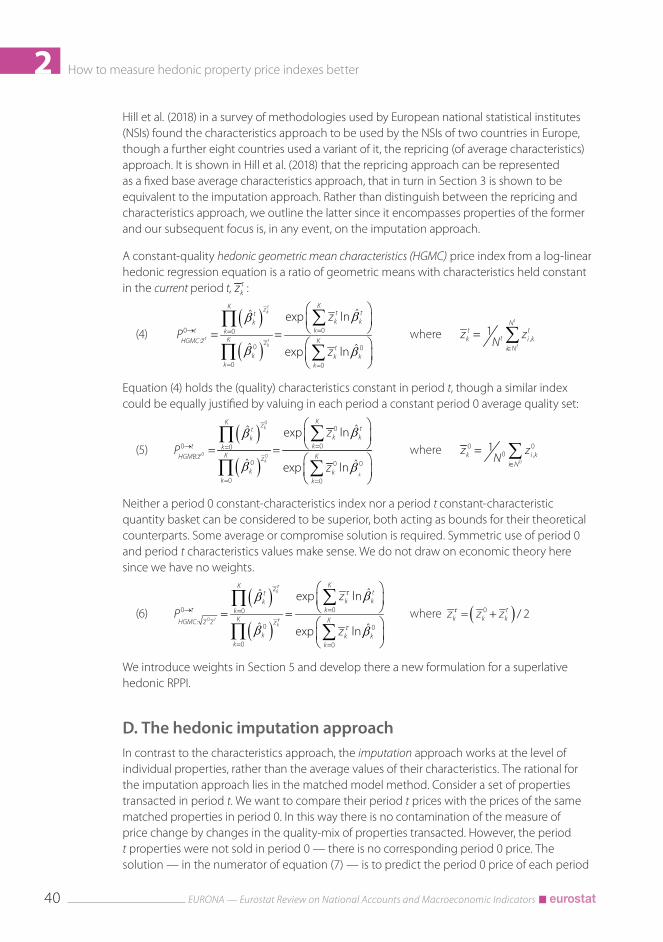
How to measure hedonic property price indexes better
EURONA — Eurostat Review on National Accounts and Macroeconomic Indicators40
2Hill et al. (2018) in a survey of methodologies used by European national statistical institutes (NSIs) found the characteristics approach to be used by the NSIs of two countries in Europe, though a further eight countries used a variant of it, the repricing (of average characteristics) approach. It is shown in Hill et al. (2018) that the repricing approach can be represented as a fixed base average characteristics approach, that in turn in Section 3 is shown to be equivalent to the imputation approach. Rather than distinguish between the repricing and characteristics approach, we outline the latter since it encompasses properties of the former and our subsequent focus is, in any event, on the imputation approach.
A constant-quality hedonic geometric mean characteristics (HGMC) price index from a log-linear hedonic regression equation is a ratio of geometric means with characteristics held constant in the current period t, t
kz :
(4)
( )
( )0 00
:0 0
0 0
ˆˆ exp ln
ˆ ˆexp ln
tk
t tk
KK z t ttk kk
t kkK KHGMC z z
tk k k
k k
zP
z
ββ
β β
→ ==
= =
= =
∑∏
∏ ∑ where ,
1t
t
Nt t
tk i ki N
z zN
∈
= ∑
Equation (4) holds the (quality) characteristics constant in period t, though a similar index could be equally justified by valuing in each period a constant period 0 average quality set:
(5) ( )
( )
0
0 0
0
0 00:
0 0 0
0 0
ˆˆ exp ln
ˆ ˆexp ln
k
k
k
KK z ttk kk
t kkK KHGMB z z
k kk k
zP
z
ββ
β β
→ ==
= =
= =
∑∏
∏ ∑ where
0
0 00 ,
1k i k
i N
z zN
∈
= ∑
Neither a period 0 constant-characteristics index nor a period t constant-characteristic quantity basket can be considered to be superior, both acting as bounds for their theoretical counterparts. Some average or compromise solution is required. Symmetric use of period 0 and period t characteristics values make sense. We do not draw on economic theory here since we have no weights.
(6) ( )
( )0
0 00
:0 0
0 0
ˆˆ exp ln
ˆ ˆexp ln
k
tk
KK z ttk kk
t kkK KHGMC z z z
k k kk k
zP
z
τ
τ
τ
τ
ββ
β β
→ ==
= =
= =
∑∏
∏ ∑ where ( )0 / 2t
k k kz z zτ = +
We introduce weights in Section 5 and develop there a new formulation for a superlative hedonic RPPI.
D. The hedonic imputation approachIn contrast to the characteristics approach, the imputation approach works at the level of individual properties, rather than the average values of their characteristics. The rational for the imputation approach lies in the matched model method. Consider a set of properties transacted in period t. We want to compare their period t prices with the prices of the same matched properties in period 0. In this way there is no contamination of the measure of price change by changes in the quality-mix of properties transacted. However, the period t properties were not sold in period 0 — there is no corresponding period 0 price. The solution — in the numerator of equation (7) — is to predict the period 0 price of each period

How to measure hedonic property price indexes better
EURONA — Eurostat Review on National Accounts and Macroeconomic Indicators 41
2t property. We use a period 0 regression to predict prices of properties sold in period t to answer the counterfactual question: what would a property with period t characteristics have sold for in period 0?
A constant-quality hedonic geometric mean imputation (HGMI) price index is a ratio of the geometric means of prices of individual properties in period t compared with period 0 of properties transacted in the current period t. The value in the numerator of equation (7) is the geometric mean of the period t price of period t price-determining characteristics, ,
ti kz . This
is compared, in the denominator, with the geometric mean of the period 0 predicted price of the self-same period t price-determining characteristics, ,
ti kz . For each property, the quantities
of characteristics are held constant in period t, ,ti kz ; only the characteristic prices change.
Where Nt is the number of properties transacted in period t:
(7) ( )( )
1
01:
00
1 ˆexp lnˆ
1 ˆexp lnˆ
t
ttii tt
ti
t
ttii tt
tt Nt i zi z
t i Ni NHGMI z
Nt i zi z
i Ni N
ppN
P
pp N
→ ∈∈
∈∈
= =
∑∏
∑∏
And a constant period 0 characteristics, 0iz , hedonic imputation HGMI where N0 is the
number of properties transacted in period 0 is given by:
(8) ( )( )
0
0000
0
0
0000
1
00
1:00
0
1 ˆexp lnˆ
1 ˆexp lnˆ
ii
i
ii
tt Ni zi z
t i Ni NHGMI z
Ni zi z
i Ni N
ppN
P
pp N
||→ ∈∈
||∈∈
= =
∑∏
∑∏
DUAL IMPUTATIONS
A natural question arises as to the phrasing of the predicted prices in equations (4) to (8) as dual imputations, that is they use predicted (imputed) prices in both the denominator and numerator — Silver (2001) and de Haan (2004a).
Dual imputation requires a predicted (imputed) price in both the denominator and numerator of equations (7) and (8), and for that matter equations (4), (5) and (6). For example, in equation (7) the single imputation index could be defined to use the actual price in the numerator and predicted price in the denominator. The denominator is a counterfactual price that a transacted property in period t would have sold for in period 0; a hedonic regression in period 0 is required. The logic for the need for dual imputations arises from the possibility of substantial omitted variable bias in the hedonic specification. For example, some cheaper terraced (row) houses may have no front garden, as they open directly onto the street. This poorer feature would be reflected in the actual price (numerator) of a constant period t index, but may be excluded or not properly represented in the hedonic specification and thus predicted price (denominator), unless a separate dummy variable: ‘no front garden’ is included in the hedonic regression. Without the new dummy variable the denominator would be biased upwards and the index downwards. The dual imputation hedonic index may to some extent offset any such upward bias by using predicted prices in both the numerator and denominator. Dual imputations are generally advised for hedonic price indexes, see: Silver and Heravi (2001); Silver (2004); de Haan (2004a); Hill and Melser (2008); Diewert, Heravi and Silver (2009); associated comments, de Haan (2009) and response, Hill (2013); and de Haan and Diewert (2013).

How to measure hedonic property price indexes better
EURONA — Eurostat Review on National Accounts and Macroeconomic Indicators42
2Yet, a feature of the OLS estimator is that the mean of actual prices is equal to the mean
of predicted prices: 0
0 0
0 00 0
1 1ˆi
iii N i N
p pN N∈ ∈
=∑ ∑|z and
1 1ˆ tit t
t tit ti
i N i N
p pN N∈ ∈
=∑ ∑|z
,, and similarly for the
logarithms of prices. Thus while the denominator of equation (7) must be counterfactual and use predicted prices, the numerator of equation (7) can use actual prices — see also de Haan and Diewert (2013), paragraph 5.38. Thus, when using unweighted hedonic imputation indexes or, as we will see, characteristics hedonic indexes, there is no need to estimate hedonic regressions in each period for (7), actual prices can be used in the numerator: equation (7) becomes:
(9) ( )( )
( )( )
1 10
01 1:
00 0
1exp lnˆ
1 ˆexp lnˆ ˆ
t t
tt tii i tt t
ti
t t
tt tii i tt t
t tN Nt i zi z i z
t i Ni N i NHGMI z
N Nt i zi z i z
i Ni N i N
pp pN
P
pp p N
→ ∈∈ ∈
∈∈ ∈
= == =
∑∏ ∏
∑∏ ∏
This is an important result since, using the principles and practice extolled in Section 5, it aids the practical work of compilers, especially in thin housing markets not to have to estimate a hedonic regression equation in each period, but maybe once a year, or every two years and chain the resulting RPPIs together. We return to this issue in Sections 4 and 5 where weighting is considered and double imputation is more problematic.
E. An indirect approach to hedonic price indexesThe indirect approach is not new, as outlined in Triplett (2006). In log-linear form a constant period t hedonic imputation RPPI (8) is given by:
(10) ( )( )
( )( )
( )( )0 0
0 0
0 0
11 10
01 1 1:
0 0 0
ˆˆ ˆ
ˆ ˆ ˆ
tt t
tt tii i tt t
ti
t
ti i it
tt NN Ni zi z i z
t i Ni N i NInGMI z
N N Ni z i z i z
i N i N i N
pp pP
p p p
→ ∈∈ ∈
∈ ∈ ∈
= =
∏∏ ∏
∏ ∏ ∏
In calculating equation (10) we take the change in average prices in the numerator and divide it by the characteristics volume change between periods 0 and t, holding the marginal valuations of these characteristics constant in period 0. This yields a price index with quality characteristics held constant at current period values. A price index with quality characteristics held constant at reference period values can be similarly defined. The time dummy method is an implicit indirect approach measuring the change in average prices (the intercept shift) having controlled for the change in characteristics. De Haan (2004b) and Diewert, Heravi, and Silver (2009) show the equivalence of this indirect hedonic characteristics index to a hedonic time dummy one.
(8) An indirect hedonic characteristics RPPI would take the form of a re-pricing index, see Hill et al. (2018).

How to measure hedonic property price indexes better
EURONA — Eurostat Review on National Accounts and Macroeconomic Indicators 43
2
3. Some equivalencesThe three approaches have different, yet valid, intuitions. Yet, as long as the functional form of the aggregator is aligned to the hedonic regression in the manner shown in Table 2.1 below, the imputation and characteristics approaches yield the same result. This consolidation not only markedly narrows down the choice between approaches but validates the measure as one resulting from quite different intuitions.
Table 2.1: Equivalences of hedonic approachesHedonic regression:
functional formCharacteristics approach:
form of average of characteristicsImputation approach:
form of average of predicted prices
Linear Arithmetic mean Arithmetic meanLog-linear Arithmetic mean Geometric meanLog-log Geometric mean Geometric mean
For a log-linear functional form of a hedonic regression, the requirements are that (i) for the characteristics approach, 0
kz and tkz are arithmetic means of characteristic’s values, the
right-hand-side (RHS) of the hedonic regression, and (ii) for the imputation approach, the ratio of average predicted prices is a ratio of geometric means, the left-hand-side (LHS). Similar equivalences shown in Table 2.1 apply to linear and log-log forms. While Hill and Melser (2008) confine the equivalences to the log-linear hedonic model, they identify the same property:
T3 [a geometric mean of geometric Laspeyres and geometric Paasche hedonic indexes] … has attractive properties when the hedonic takes the log-linear form. The fact that it can be defined in either goods or characteristics space adds flexibility to the way the results can be interpreted. For example, T3 can be interpreted either as measuring the average of the ratios over the two region-periods of the imputed price of each house or as the ratio of the imputed price of the average house. Which perspective is most useful may depend on the context. Hill and Melser (2008, pp. 602).
A log-linear hedonic characteristics price index with constant reference-period average
characteristics, 0
0 00 ,
1k i k
i N
z zN
∈
= ∑ , equals an imputation index for reference period properties:
(11) ( )
( )
0
0
0
0
0 0
0
00,
00 00:
0 0 0 0 0,
0 0 0
1
1
ˆˆˆ exp lnexp ln
ˆ ˆ ˆexp ln exp ln
k
i k
KKK z ttti k kk kk
kt k i NkK KHGMI z Kz
k k k i k kk k k i N
N
N
zzP
z z
βββ
β β β
=→ = ∈=
= = = ∈
= = =
∑∑∑∏
∏ ∑ ∑∑
( )( )
0
0
0
00 0
0
00 0
10,
01
0 0 0,
0
1
1
ˆexp ln ˆ
ˆexp ln ˆ
i
i
Kt t N
i k k i zki N i N
KN
i k k i zki N i N
N
N
z p
z p
β
β
|=∈ ∈
|=∈ ∈
= =
∑∑ ∏
∑∑ ∏
and similarly, average characteristics held constant in the current period t, ,1
t
t ttk i k
i N
z zN
∈
= ∑ is equal to an imputation index for current period t properties:
(12) ( )
( )
( )( )
1
0 01:
0 0
0
ˆ ˆ
ˆ ˆ
ttk
tit
t ti k t
tit
K z tt Nk i z
t k i NKHGMI z z
Nk
i zk i N
pP
p
β
β
|→ = ∈
|= ∈
= =∏∏
∏ ∏

How to measure hedonic property price indexes better
EURONA — Eurostat Review on National Accounts and Macroeconomic Indicators44
2
4. Weights and superlative hedonic price indexes
(9) Griliches (1961, 1964) revived the hedonic approach to the construction of price indexes. Griliches (1971) raised methodological issues that foreshadowed many of the issues of concern in this paper including the need for weighting in regression estimates and the empirical form of the relationship, commenting on the preferred use of the semi-logarithmic form.
(10) Rambaldi and Rao (2013) provide details on hedonic price indexes using democratic (equal) weights as opposed to plutocratic (stock or expenditure-share) weights.
A. Weights in a hedonic RPPISo far we have made no mention of an essential element of index number construction: the weighting of price changes. If one index number formula has a superior weighting, other things being equal, it is preferred. As noted by Griliches (1971, pp. 326): There is no good argument except simplicity for the one-vote-per-model approach to regression analysis (9).
We distinguish between two levels of aggregation: the lower and higher levels. Property price indexes are often stratified by type and location to form more homogeneous strata of properties, say apartments in the capital city. The national or some higher-level index is compiled as a weighted average of the constant-quality price changes of the individual strata indexes. These higher-level strata are very broad, designed to ensure a large sample size is available for the estimation of hedonic regressions within them. At the lower or elementary level constant-quality price indexes are estimated for each stratum, generally as unweighted, that is equally-weighted, indexes. That say a price change of a three-bedroom apartment in an up-market area of a capital city should have the same weight as that of a studio apartment in a down-market area goes against the well-accepted principles, as embodied in international measurement standards (Eurostat et al. (2013), of expenditure-weighted price index numbers. Given the heterogeneity of price changes within these broad strata the absence of weighting systems at the lower level, within strata — at the level of the price change of the individual property — is a major shortcoming. To the author’s knowledge no statistical office currently successfully uses weights except at the crudest higher level.
Weights at the higher and lower levels, as described in Silver (2016), can be the relative values of transactions or stocks of properties for each stratum (10). This choice between the use of ‘transactions’ or ’stocks’ as weights depends on the purpose of the property price index and availability of adequate data on the stock of properties. Fenwick (2013) and Mehrhoff and Triebskorn (2016) outline issues relevant to such a choice, though the concern here is with the methodology for incorporating weights into the lower level within stratum RPPI measurement.
There is literature on elementary price index number formulas based on the needs of consumer, producer and trade price indexes. While some of these results have a bearing on the analysis here, the context differs in important respects. First, the matched prices are predicted constant-quality prices for individual properties. Second, an individual property sold in the reference (current) period has as its matched price in the current (reference) period a counterfactual predicted price. Third, the weight to be attached to each property’s price

How to measure hedonic property price indexes better
EURONA — Eurostat Review on National Accounts and Macroeconomic Indicators 45
2change is its relative expenditure, that is, its price. Fourth, the elementary property price indexes are constant-quality indexes that make use of hedonic (or repeat sales) regressions. The weights given to the property price observations, for a time dummy method, are implicit in the way observations of prices enter into the regression or aggregation formula. We provide an improved mechanism for weighting at this lower elementary level.
In this section we consider three issues which allow us to develop a hedonic superlative price index number; in Section 4B we develop a proposed method for weighting hedonic property price indexes to form what we term as ‘quasi-superlative indexes’. Superlative price index number formulas are less likely to suffer from substitution bias, a bias that results when a single-period fixed basket index is used to estimate a cost of living index. The bias arises because a fixed basket index cannot take account of the effects on the cost of living of the substitutions made by consumers in response to changes in relative prices. In general, the earlier the period of which the basket is used, the greater the upward bias in the index.
Section 4C provides a definition of hedonic superlative price indexes and shows how they differ from the ‘quasi’ formulations in terms of an absence of sample selectivity bias. The quasi-superlative and superlative RPPIs defined in Sections 4B and 4C are derived from a hedonic imputation approach. Section 4D provides equivalent derivations from a hedonic characteristics approach. The formulations derived in Sections 4B and 4C differ from accepted wisdom and in Section 4E we use the, in many ways, seminal paper by Hill and Melser (2008) to show how this formulation improves on the one they advocate, which has been used by others in much subsequent work. In Section 4F we turn to a problem in using weights for the time dummy approach.
B. Quasi-superlative hedonic RPPIsConsider again equation (8); the index is a measure of price change for constant-period 0 characteristics property price indexes:
(13) ( )( )
0
0000
0
00 0
0
11
01 0:
0
ˆ ˆ
ˆ
ii
i
i
t Nt Ni zi zt i N
HGMI zi NN i z
ii N
p pP
pp
||→ ∈
∈ |
∈
= =
∏∏
∏
There are three problems with this measure: (i) property price changes are equally weighted; (ii) the index is based on only the sample of properties transacted in period 0; and (iii) the introduction of explicit weights precludes our previous use of equating average predicted prices to average actual prices, as a means by which dual imputations are introduced. We consider each in turn.
The first task is to apply weights to these price changes. A useful opportunity exists using the imputation approach to explicitly introduce weights at this very lowest level. This approach, to the author’s knowledge, was first proposed in Feenstra (1995) and used by Ioannidis and Silver (1999) in an application, using scanner data, of hedonic methods to quality adjust price indexes for television sets, in Silver and Heravi (2007a), further developed in Diewert, Heravi, and Silver (2009), and in the context of RPPIs, in Hill and Melser (2008).
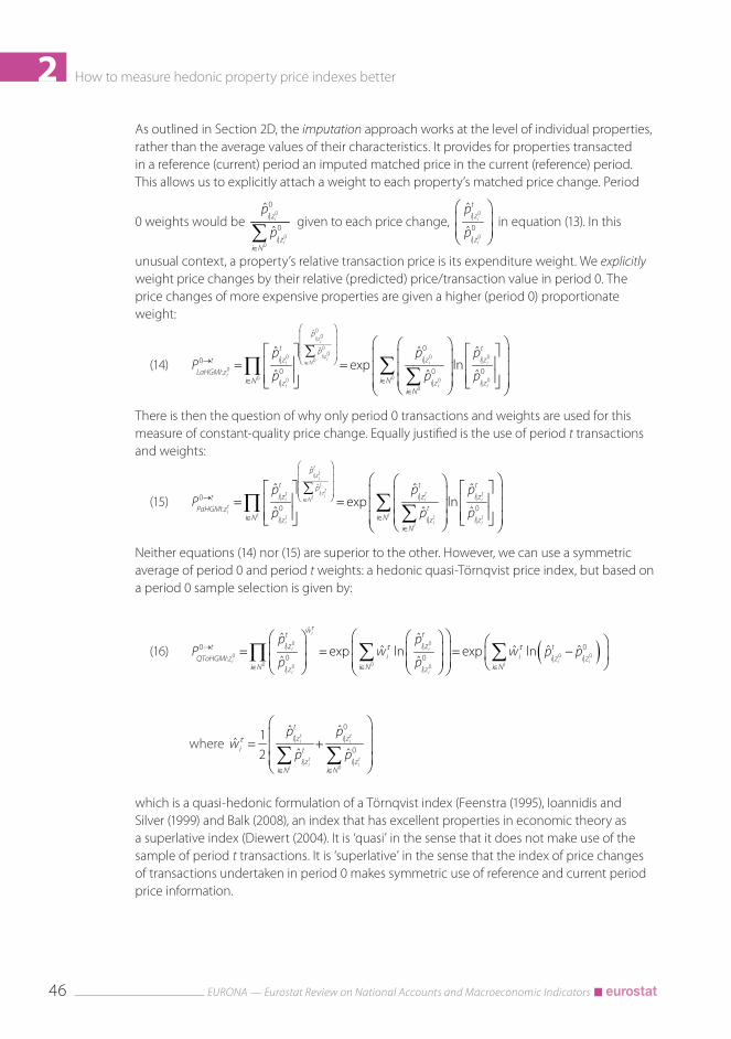
How to measure hedonic property price indexes better
EURONA — Eurostat Review on National Accounts and Macroeconomic Indicators46
2As outlined in Section 2D, the imputation approach works at the level of individual properties, rather than the average values of their characteristics. It provides for properties transacted in a reference (current) period an imputed matched price in the current (reference) period. This allows us to explicitly attach a weight to each property’s matched price change. Period
0 weights would be 0
0
0
0
0
ˆ
ˆi
i
i z
i zi N
p
p|
|∈∑
given to each price change, 0
00
ˆ
ˆi
i
t
i z
i z
p
p|
|
in equation (13). In this
unusual context, a property’s relative transaction price is its expenditure weight. We explicitly weight price changes by their relative (predicted) price/transaction value in period 0. The price changes of more expensive properties are given a higher (period 0) proportionate weight:
(14)
00
00
0 0 00
0
00 0 0 0
0
ˆ
0ˆ0
0 0 0:
ˆ ˆ ˆexp ln
ˆ ˆ ˆ
i zi
i zii i ii N
i
i i i
p
t tpi z i z i zt
LaHGMI zi Ni N i z i z i z
i N
p p pP
p p p
|
|∈
| | |→
∈∈ | | |∈
∑ = =
∑∏ ∑
There is then the question of why only period 0 transactions and weights are used for this measure of constant-quality price change. Equally justified is the use of period t transactions and weights:
(15)
ˆ
ˆ0
0 0:
ˆ ˆ ˆexp ln
ˆ ˆ ˆ
tti zit
ti zt t titi i ii Nti tt t t t
i i it
p
t t tpi z i z i zt
tPaHGMI zi Ni N i z i z i z
i N
p p pP
p p p
|
|∈
| | |→
∈∈ | | |∈
∑ = =
∑∏ ∑
Neither equations (14) nor (15) are superior to the other. However, we can use a symmetric average of period 0 and period t weights: a hedonic quasi-Törnqvist price index, but based on a period 0 sample selection is given by:
(16) ( )0 0
0 0 0
00 0 0
ˆ
0 00 0:
ˆ ˆˆ ˆˆ ˆexp ln exp ln
ˆ ˆ
i
i i
i i iti i
wt t
i z i zt ti iQToHGMI z i z i z
i N i Ni N i z i z
p pP w w p p
p p
τ
τ τ| |→| |
∈ ∈∈ | |
= = = − ∑ ∑∏
where
0
0
0
ˆ ˆ1ˆ
ˆ ˆ2
t ti i
t ti it
t
i z i zi t
i z i zi N i N
p pw
p pτ | |
| |∈ ∈
= + ∑ ∑
which is a quasi-hedonic formulation of a Törnqvist index (Feenstra (1995), Ioannidis and Silver (1999) and Balk (2008), an index that has excellent properties in economic theory as a superlative index (Diewert (2004). It is ‘quasi’ in the sense that it does not make use of the sample of period t transactions. It is ‘superlative’ in the sense that the index of price changes of transactions undertaken in period 0 makes symmetric use of reference and current period price information.

How to measure hedonic property price indexes better
EURONA — Eurostat Review on National Accounts and Macroeconomic Indicators 47
2Equation (16) uses a period 0 sample of transactions. A similar quasi-hedonic Törnqvist index based on period t transactions is given by:
(17) ( )ˆ
0 00 0:
ˆ ˆˆ ˆˆ ˆexp ln exp ln
ˆ ˆ
i
t ti i
t t ti i it tt t t
i i
wt t
i z i zt ti iQToHGMI z i z i z
i N i Ni N i z i z
p pP w w p p
p p
τ
τ τ| |→| |
∈ ∈∈ | |
= = = − ∑ ∑∏
These innovative quasi-hedonic superlative formulas depart from conventional hedonic formulations — Diewert (2003), de Haan (2004a), Silver and Heravi (2005), de Haan and Krsinich (2014, Appendix A) — in which the weights attached to each price change for transactions in period 0 are the relative expenditures in period 0 (for 0i N∈ ) and for period t are the relative expenditures in t, (for ti N∈ ), as opposed to an average of period 0 and t, as in equations (15) and (16).
We note that in using equations (14) to (17), we have a comparison between predicted prices in period 0 and counterfactual predicted prices in period t. We can no longer rely on the OLS property of average predicted prices equalling average actual prices to achieve double imputation. This need to undertake a hedonic regression each current period for equation (16) is revisited in Section 7 with a workaround. We also note that given these predicted prices act as corresponding weights in period t for the price change, it would be wasteful to abandon the thought experiment for the weights but not for the price change. Indeed, abandoning ˆ iwτ in favour of iwτ would remove the analytical power of taking some account of substitution
bias.
C. Hedonic superlative indexes and sample selection biasThe quasi-Törnqvist indexes in equations (16) and (17) were each based on samples of period 0 and t transactions respectively. In both cases, the distinction is not one of substitution bias; it is a sample selection bias. Substitution bias arises, in this context, from using period 0 or period t weights, rather than a symmetric mean of the two period’s expenditure weights, as in a Törnqvist index. The quasi-superlative formulas outlined above make symmetric use of both periods’ weights, but limits the sample to transactions in either period 0 or period t. Our hedonic Törnqvist price index should be based on samples of period 0 and period t transactions.
Some additional notation may help clarify the formulas. Let ( )0S t∩ be the set of properties that are transacted in both periods 0 and t, ( )0S t¬ is the set of properties transacted in period 0 but not period t, and ( )0S t¬ is the set of properties that are transacted in period t but not period 0. The weights for each term are the relative transaction values of these sets of data, that is, where V is the total value of transaction prices (or stocks) for ( )0S t∩ , ( )0S t¬
and ( )0S t¬ , ( 0) (0 ) (0 ) ii S t S t S t
V v∈ ¬ ∩ ¬ ∩ ∩
=∑ ; 0 0t ii tv v¬ ∈ ¬
=∑ ; 0 0t ii tv v¬ ∈¬
=∑ ; and 0 0t ii tv v∩ ∈ ∩
=∑
and iwτ is an arithmetic mean of the weight (relative stock value or transaction (price) value) given to each property in periods 0 and t, that is ( )0ˆ ˆ ˆ1 2 t
i i iw w wτ = + . Bear in mind that we are weighting the price change of each individual property and the weight is the relative

How to measure hedonic property price indexes better
EURONA — Eurostat Review on National Accounts and Macroeconomic Indicators48
2expenditure that equates to the price of the property. In this unusual situation we can use
predicted prices for weights, as argued above:
( ) ( )
( )0
00
0 0
ˆ ˆ1 1ˆ ˆ ˆ
ˆ ˆ2 2
t ti i
t ti i
t
i z i z ti i it
i z i zi S t i S t
p pw w w
p pτ | |
| |∈ ¬ ∈ ¬
= + = + ∑ ∑
.
The hedonic Törnqvist price index is:
(18) ( ) ( ) ( )
0 00
, ,
ˆ ˆˆ
00 0 0:
0 0 0
ˆ ˆ ˆ
ˆ ˆ ˆ
t tti ii
t t ti i i
it t ti i k i k
v vvw wwt t tV VV
i z i z i zt
ToHGMI zi S t i S t i S ti z i z i z
p p pP
p p p
τ ττ
τ
¬ ∩¬ × ××
| | |→
∈ ¬ ∈ ¬ ∈ ∩| | |
= × ×
∏ ∏ ∏
The superlative Törnqvist hedonic price index follows Triplett and McDonald (1977), Diewert (2003), Triplett (2006), de Haan (2004a), and Silver and Heravi (2005) (11). We note that for repeat sales, (0 )S t∩ , we have used a double imputation, that is predicted prices, when actual prices are available. At first sight this goes against the principles of matched models measurement whereby actual prices are compared, say for the price change of a single standard can of Coca-Cola for a consumer price index, the price is compared over time like with like. However, as Hill and Melser (2008) explain:
As far as we are aware, the possibility of always imputing for a repeat observation … has not previously been considered in the literature. For the case of computers, this would be hard to justify since a particular model is the same irrespective of when it is sold. Housing, however, is another matter. There is no guarantee even for a repeat sale that we are comparing like with like. This is because the characteristics of a house may change over time due to renovations or the building of a new shopping center nearby, etc. The only way to be sure that like is compared with like is to double impute all houses (even with repeat sales). Hill and Melser (2008, pp. 600).
Equation (18) has the following features:
• Its general form is a Törnqvist index, a superlative price index — an index number formula with good approximation to a price index without substitution bias.
• It has no sample selectivity bias in that it includes estimates of constant-quality price change using three sets of price observations: (i) transacted in period 0 (but not in period t); (ii) price observations transacted in period t (not in period 0); and (iii) repeat price transactions available in both periods 0 and t.
• The aggregate of each term, that is each set of transactions, is weighted by the expenditure share of that set, for example, if there are few repeat transactions in periods 0 and t, these price changes have a commensurately less weight. This is appropriate for a sample selection issue (12).
(11) This paper acknowledges the contribution from Erwin Diewert (University of British Columbia) who helpfully provided rigorous derivations of these results in a previous working version of Silver and Heravi (2005).
(12) This inclusion of transactions confined to periods 0, t and both periods is akin to issues faced in productivity measurement, with entering, exiting and continuing firms, and cost-of-living measurement with new, obsolete and continuing products as is particularly apparent with the emergence of the digital economy, see Diewert and Feenstra (2017) and Reinsdorf and Schreyer (2017).

How to measure hedonic property price indexes better
EURONA — Eurostat Review on National Accounts and Macroeconomic Indicators 49
2• A dual imputation is used for the constant-quality price change measurement for the
weights and relative predicted values.• We outline later some practical advantages of using a form of equation (16). What is apparent
here is that equation (16) has a sample selectivity bias, but one that can be retrospectively tested by comparison with equation (18), in which it is identified here as a component.
D. And what about a weighted characteristics hedonic index?As long as we adopt appropriate aggregators and functional forms as outlined in Table 2.1, the imputation and characteristics methods give the same result. This holds for weighted and unweighted versions. Were a weighted characteristics approach taken the weights would be introduced, for each transaction, in the measure of the arithmetic mean of the characteristics.
(19) 0
0
0
0
0 0,
00
ˆ
ˆ
i
i
i ki zi N
k
i zi N
p zz
p
|∈
|∈
=∑∑
and ,ˆ
ˆ
tit
tit
t ti ki z
t i Nk t
i zi N
p zz
p
|∈
|∈
=∑∑
The view taken here is that the RPPIs should be weighted and especially so given there is no lack of information for weights at the elementary level. It is more intuitive to compile price indexes as weighted averages of price changes, rather than characteristic values. Thus, the weighted imputation approach is recommended.
E. Alternative hedonic superlative price index number formulasOur formulation of a hedonic superlative index, equation (18), differs from Hill and Melser (2008) — hereafter HM — reiterated in Hill (2013) and used by Rambaldi and Rao(2013) (13). HM (2008, pp. 601-602) derive hedonic Fisher and Törnqvist hedonic price indexes from the imputation and characteristics approach for a semi-logarithmic functional form of a hedonic regression. In an important contribution, they first show how the derivations from the two approaches provide the same results. Second, they solve the absence of matched models (infrequent transactions) by separately considering geometric Laspeyres (for constant period 0 characteristics) and geometric Paasche indexes (for constant period t characteristic), and then taking a geometric mean of the two to derive a superlative hedonic price index. We show both of these below but take issue with their formulation of a hedonic superlative price index compared with our equation (18).
HM (2008, pp. 601) define a geometric, period 0 sample hedonic price index as:
(20)
00
00
00 0
0
0 00 00 0
ˆ ˆ
ˆ ˆ
i zii
i zii ii N
i i
pwt tp
i z i z
i N i Ni z i z
p p
p p
|
|∈
| |
∈ ∈| |
∑ =
∏ ∏ where 0 0
0
0 0 0
i ii i z i z
i N
w p p| |
∈
= ∑
(13) De Haan and Diewert (2013) in the RPPI handbook, Eurostat et al. (2013) have a similar formulation to Hill and Melser (2008) except that it is unweighted.

How to measure hedonic property price indexes better
EURONA — Eurostat Review on National Accounts and Macroeconomic Indicators50
2A geometric, period t index is similarly defined and a superlative formulation is a geometric mean of the period 0 and period t hedonic indexes:
(21) ( ) ( )
0
0
00 0
0 0
ˆ ˆ
ˆ ˆ
ti i
ti i
tii
w wt ti z i z
i S t S t i zi z
p p
p p| |
∈ ¬ ¬ ||
×∏ ∏
This formulation differs from the one proposed in equation (18) in some important respects, including — further points and detail are in Silver (2016): (i) the HM formulation captures the samples of transactions in periods 0 and t, but it does not include the symmetric weights of each transaction, and thus cannot take account of substitution effects; (ii) price changes of period 0 transactions are weighted by 0
iw and price changes of period t transactions by tiw , as
opposed to ˆ iwτ and (iii) the sets of the price changes, ( )0S t¬ and ( )0S t¬ , are not weighted according to their sample sizes. A symmetric mean is taken akin to a superlative index.
F. Use of a weighted least squares (WLS) estimator for the hedonic regression if weights are to be applied in aggregationFinally, a neglected issue for the imputation (and characteristic) approach is the use of a weighted least squares (WLS) estimator for the hedonic regression. Diewert (2005a) in a seminal paper on weighted aggregation in hedonic regression indexes argued for a WLS estimator using expenditure shares as weights. Diewert (2005a) showed that for a bilateral two-period aggregate price comparison with average expenditure shares ( ),0 , 2/i i tw w+ used as weights in a WLS estimator, the estimated price change is equivalent to the superlative Törnqvist index (14). There are two main reasons why this may not work.
LEVERAGE, INFLUENCE, AND ROBUST ESTIMATORS
Silver (2005, Appendix 1) and Silver (2016, Annex 2) (15) raised a concern that observations may have undue influence in a regression for reasons unrelated to their weighting. In a time dummy hedonic regression a property price observation whose characteristics differ markedly from their means — have a relatively high leverage — and whose price is not well predicted by the regression — has a relatively large residual — can have a weight/influence in determining the constant-quality price change that is markedly greater than merited by its singular transaction in OLS or expenditure (price) share in WLS. For example, an atypical six-bedroom (larger) house with high leverage may also have a high residual from the regression, and thus influence in determining the regression coefficients, in spite of expenditure shares being possibly minimal. This undue influence applies even when expenditure-share WLS is used as an estimator.
(14) Further contributions on developing (value-share) weighting systems in regression-based estimates of aggregate price change include Feenstra (1995), Ioannidis and Silver (1999), de Haan (2004 and 2009), Diewert, Heravi and Silver (2009), Ivancic, Diewert, and Fox (2011) and de Haan and Krsinich (2014), and for the cross country-product dummy approach, see Rao (2005).
(15) Much of this is drawn from a 2002 unpublished mimeo by the author, Cardiff University.

How to measure hedonic property price indexes better
EURONA — Eurostat Review on National Accounts and Macroeconomic Indicators 51
2The problem is not just one of observations with high influence having a disproportionate effect on the estimated coefficients and predicted values. High-end properties with low residuals lying on the estimated hedonic surface will have little to no influence on the estimated coefficients, in spite of what may be relatively high expenditures.
Influence statistics, such as Cook’s distance, are a method of discovering influential observations in a multivariate framework. Measures of leverage and residuals are readily available in econometric software (16) and may be used to investigate and remove observations with unduly high influence, but such a process may not be regarded as ’arms-length’.
An alternative approach to the treatment of observations with undue influence (weight) is to use a heteroscedastic-consistent covariance matrix estimator (HCCME). For example, the HC2 estimator replaces the squared OLS residuals 2ˆ iµ by a term that includes the leverage — see also the HC4 estimator proposed by Cribari-Neto (2004) (17). The ith residual is inflated more (less) when its leverage, ih , is large (small) relative to the average of the ih , which is k n , see MacKinnon (2013). Such influence effects are particularly problematic with the use of WLS for the time dummy approach because both the estimation of the regression coefficients and the aggregation of the RPPI are part and parcel of the same process.
More generally, observations with undue influence — in relation to their expenditure (price) — should be detected, examined, and modified/deleted and/or a robust estimator applied with the results contrasted with those estimated by WLS.
WLS is typically used in econometrics to correct for a heteroscedastic error term to achieve more precise parameter estimates. If the error term was homoscedastic prior to weighting, the weighting will induce heteroscedasticity and imprecise estimation, Solon et al. (2015).
(16) For example, EViews 9 User’s guide (2015) provides least squares diagnostics for outlier detection, described in ’Leverage plots’, pp 218 along with six diagnostic statistics/tests of the ‘Influence of an observation’, pp 220.
(17) EViews also has routines for ’Robust least squares’ and details of three robust estimators one of which has as its focus outliers with high leverage. HC2 replaces the squared OLS
residuals with ( )
2ˆ1
i
ih
µ−
and HC4 with( )
2ˆ
1
i
iih
µδ−
where, min(4, )i inhkδ = and n is the number
of observations and k the number of explanatory variables, ˆ iµ the residuals. MacKinnon (2013) notes that a few papers have taken different approaches: Furno (1996) uses residuals based on robust regression instead of OLS residuals in order to minimise the impact of data points with high leverage, see EViews 9 User’s Guide (2015), pp. 387.

How to measure hedonic property price indexes better
EURONA — Eurostat Review on National Accounts and Macroeconomic Indicators52
2
5. Practical problem of appropriate hedonic formulas for thin markets
(18) There are other approaches to the problem of thin markets including (i) estimating a temporally aggregated price index for example, moving from a quarterly to a semiannual or annual index, Geltner (1993) and Bokhari and Geltner (2012); (ii) use of a time-series methodology, such as the Kalman Filter, including Goetzmann (1992), Francke (2008), and Rambaldi and Fletcher (2014); (iii) the inclusion of other related series as explanatory variables in thin markets, Baroni et al. (2007); and (iv) an improvement to the efficiency of the estimator using data on sample sizes, Silver and Graf (2014).
Having defined a hedonic superlative index, our concern is with the development of a best practice, well-grounded practical formula for measuring hedonic property price indexes that are suitable for property markets where properties are heterogeneous and transactions sparse — thin markets (18). It is a concern that would more generally apply to regular hedonic estimation and its vagaries of estimation and specification as would be required for real time compilation, that is, for every current period t. These proposals are grounded in the theoretical framework in the previous sections. Section 5A below reminds us of the results on equivalences and points to a preference for the hedonic imputation approach. Section 5B outlines methods that only require a hedonic regression to be estimated in the reference period, yet still manages to include approximations to a superlative index, and Section 5C outlines the use of an extended reference period in this context. There are three caveats to this: first, in Section 5D, the need for frequent re-estimation of the reference period hedonic regression is outlined and a mechanism for testing the desired frequency of the re-estimation. Second, the methods outlined in Section 5B suffer from having a single imputation; Section 5E provides a workaround and Section 5F provides guidance on estimators for the hedonic regression to be consistent with the weighting system applied.
A. Equivalences We have shown that for reasonable hedonic specifications and the use of appropriate aggregators outlined in Table 2.1 above, the hedonic characteristics and imputation approaches, and indirect approaches all yield the same result. Similar results hold for weighted variants of the measures. There is an axiomatic sense that gives credence to a measure that gives the same results when derived from different, but valid, intuitions; this helps consolidate choice. An imputation approach is proposed since it has a natural formulation when weights are applied. The application of weights requires no new data and can be readily undertaken, as outlined below. A weighted RPPI is preferable to an unweighted one.
B. A hedonic RPPI based only on an estimated regression in the reference periodThe proposed measures below are imputation RPPIs based on a current period sample of period t transactions, as outlined above. They only require a hedonic regression for period 0. Limiting the regression estimation to the reference period is a major advantage. Hedonic regression estimates are subject to the vagaries of specification and estimation procedures, particularly in thin markets. A measure based on a well-grounded regression, especially one

How to measure hedonic property price indexes better
EURONA — Eurostat Review on National Accounts and Macroeconomic Indicators 53
2based on an extended reference period as outlined below, better grounds the index. An unweighted version is equation (22) — taken from equation (7) above:
(22) ( )
( )
1
01:
00
1 ˆexp ln
1 ˆexp lnˆ
ttitt
ti
t
ttii tt
tt Nti i z
t i Ni NHGMI z
Nt i zi z
i Ni N
ppN
P
pp N
→ ∈∈
∈∈
= =
∑∏
∑∏We note that an adjustment for double imputation is not required for the unweighted version
in equation (22). This is because for an OLS regression, 1 1ˆ t
it t
t tit ti
i N i N
p pN N∈ ∈
=∑ ∑|z, and similarly for
the logarithms of prices, a feature that does not carry over to weighted counterparts. In using only a reference period, regression equation (22) is akin to the characteristics-based repricing method used by some European countries, as outlined in Hill et al. (2018). However, these repricing indexes are unweighted. Given the simplicity and efficacy of using weights, equation (22) cannot be recommended (19). Weighted versions are preferred.
A period t weighted version is equation (23) — taken from equation (15) above:
(23) 00 0:
exp lnˆ ˆ
ti
ti
ti Nti tt t t
i it
p
pt t tt i i i
tPaHGMI zi Ni N ii z i z
i N
p p pP
p p p∈
→
∈∈ | |∈
∑ = =
∑∏ ∑
A quasi-superlative version is equation (24), clearly superior to equation (23) — taken from equation (17) above:
(24)
0
0
ˆ/2
ˆˆ 020
ˆexp ln lnˆ
t
t
t t
ti zi itii z ti
i N i N ititt t
i
pp
p ptwJ ti
HIL i i zi Ni N i z
pP p p
p
|
|∈ ∈
+
|∈∈ |
∑ ∑ = = − ∑∏
where 0
0
ˆ1ˆ
ˆ2
tt i
tit t
ti zi
i ti i z
i N i N
ppw
p p|
| |∈ ∈
= + ∑ ∑
Equation (24) while only requiring the estimation of a hedonic regression in the reference period clearly provides an estimate that includes substitution effects for the sample of period t transactions. The thought experiment is of a price change of an individual house: its transaction price in period t compared to what its transaction price would have been in period 0 had it been sold then — a counterfactual price relevant to the needs of RPPI
(19) The characteristics hedonic RPPI requiring a hedonic regression only in the reference period 0 is given by the first two terms of:
( )( )
0 0
0 0
0
00ˆ 0 0 0
0 0 00
ˆexp expexp ln
ˆ ˆ ˆexp ln exp ln exp ln
tk
k
N NKK t tt tt i ik kki N i Nkk
K K KK t t ttk k k k k kk
k k kk
p pzz
z z zz
β
β
β
β β β
∈ ∈==
= = ==
∑ ∑ ∑∏ = = = ∑ ∑ ∑ ∏
Making use of equations (9) and (11), a constant period t, double-imputation, hedonic characteristics RPPI can be measured by simply taking the geometric mean of the actual prices in the numerator which is equal for an OLS regression to that of the predicted prices.

How to measure hedonic property price indexes better
EURONA — Eurostat Review on National Accounts and Macroeconomic Indicators54
2measurement. The phrasing of the weights captures the (approximate) substitution effect being relevant to the price change measured. If the prices of houses in an up-market area rise faster than other houses, the weights will reflect the shift in expenditures since they are tied to the definitions of the price change. Identical results can be derived from a characteristics approach (20).
However, while the weights are appropriate, the price change for the weighted version is a single imputation and for reasons outlined in Section 2D, a workaround is required to develop an approximation to a double imputation. We return to this in Section 5E below.
C. That an extended-current period formulation be used since sparse data is less problematicA major problem in RPPI and CPPI estimation is that of sparse data on heterogeneous properties. However, this can be alleviated by the use of an extended reference period, noted as a useful feature of property price index construction by de Haan and Diewert (2013) (21). Nonetheless, extended periods may not be used for the current period hedonic regression estimation without being to the detriment of the periodicity of the series, for example, a quarterly series becoming bi-annual. This gives further support to the case for reference-period only hedonic regression estimation such as in equations (22) to (24).
There may not be an adequate number of observations and/or variation in the characteristics of the sample of properties transacted in period 0 to enable reliable and pertinent estimates to be made of the coefficients of price-determining characteristics that define properties sold in period t. For example, there may a relatively small number of four-bedroom houses in a prime location sold in period t, but none sold in period 0. The problem of sparse data prevents reliable estimates of the predicted price from a period 0 regression of the period t characteristics (22). The current period formulation can go some way to solving the problem of sparse data simply by defining the reference period 0, for example, for a quarterly series first quarter 2018, second quarter 2018, etc., to be an extended period of say a year with the index referenced as 2017 = 100.0 and centred at mid-2017. As such, the period 0 regression will be more likely to better encompass the characteristics of period t properties.
The advantage of not having to re-estimate a hedonic regression on a periodic basis is well recognised by NSIs in Europe. The repricing variant of the characteristics approach used by eight countries has an extended reference period of a year to establish the average values of the characteristics and the commensurate estimated marginal values from the hedonic regression. The repricing approach allows for this due to its correspondence to the characteristics approach and equivalence to the imputation approach when crafted following the principles in Table 2.1. We continue with the imputation approach.
(20) The interpretation of the characteristics approach is problematic, thus the focus on the imputation approach.
(21) Though de Haan and Diewert (2013) refer to it in the context of an advantage of the indirect method, similar such formulations and advantages apply to the direct imputation and characteristics approach.
(22) More formally, the width (standard error) of a prediction interval from a regression ofony x , for a given value of say x x′= , depends not only on the fit of the regression
— the larger the sample size and dispersion of the explanatory variables, the smaller the interval — but also on the distance the given value of x′ is from the sample mean x . The prediction will be better for values of x′ closer to x , see Maddala and Lahiri (2009).

How to measure hedonic property price indexes better
EURONA — Eurostat Review on National Accounts and Macroeconomic Indicators 55
2D. Sample selectivity biasSince the sample of period t transactions is only used, there may be a sample selectivity bias as explained in Section 4C. Yet equation (18) is a measure of a superlative Törnqvist RPPI for the complete period t sample of transactions; it is quasi-superlative. It would be a relatively trivial matter for a retrospective study to be conducted prior to the adoption of the methodology that compares the results of equation (24) with (18) to ascertain the extent and direction of any such bias. Sample selection bias can be mitigated by frequent re-estimation of the hedonic regression, say every year or two years, and chain-linking the results. This would be akin to rebasing a consumer price index to introduce new weights.
E. Dual imputations of price relatives: a workaroundEquations (23) and (24) differ from their counterpart equations (15) and (17) in that the measure of price change in the latter use dual imputations while the former uses a single imputation. This deficiency in equations (23) and (24) arise from the simple fact that our intention is to avoid estimation of a hedonic regression in the current period. The single imputations in equations (23) and (24) require workarounds so that approximations to predicted prices are used instead of actual prices. Define weights as:
(25) 0
0
0
0 0
0 0 00 0 0
0 0 0
ˆ ˆˆ ˆ; ; ;
ˆ ˆ
ti i
ti i
ti it t
ti z i z ti i
i i ti z i zi ii z i z
i N i N i N i N
p p p pw w w w
p p p p| |
| || |
∈ ∈ ∈ ∈
= = = =∑ ∑ ∑ ∑
A workaround for the predicted value of period t prices for a dual imputation can be seen from equation (26):
(26) ( )
( )( )( )
( )( )
00
0
0
0 0 0
0
ˆ ˆ0
ˆ ˆ00 0
ˆ ˆ
ˆ ˆ
ttti i z i zi i
ti it t
t i ti z i zi it ti it t
w wwt ti i z i z
J i N i N i NHIGL w w w
ii z i zi Ni N i N
p p pP
pp p
| |
| |
| |∈ ∈ ∈
| |∈∈ ∈
= × ≠∏ ∏ ∏
∏∏ ∏
The first term is the single imputation, ‘adjusted’ by the second term which is the ratio of the geometric mean of predicted values in period 0 to that of actual values in period 0, a term readily compiled from the real time data since we have estimated a regression in period 0. This is not equal to our desired measure, the third term in equation (26), but should be a close approximation. The desired expression is the period t ratio of predicted to actual values, that is we are assuming:
(27)
( )( )
( )( )
00
0
0
0
0
ˆ ˆ0
ˆ 0
ˆ ˆt
ti z i zi iti it
ti i
t
w wt
i z i zi N i N
w wti i
i N i N
p p
p p
| |
| |∈ ∈
∈ ∈
=∏ ∏
∏ ∏

How to measure hedonic property price indexes better
EURONA — Eurostat Review on National Accounts and Macroeconomic Indicators56
2The validity of the assumption can be examined over time as the hedonic regression is updated; the more frequent the updates, the more likely the double-imputation workaround is likely to hold. The workaround in equation (26) can also be justified using the indirect method; that is we divide the change in actual average prices by the change in the characteristic mix (23):
(28)
( )
( )
( )( )
( )
( )( )( )
( )( )
000
00 0
0 0 00
0
00
0
0
ˆ ˆ0 0
ˆ ˆˆ 00 00
ˆ0
ˆ ˆ
ˆ ˆˆ
ˆ
ti
t
ttti i i z i zi i
ti it t
t i tt i z i zi z i iit tti ii tt
i zi
i
wti
i Nw ww wt t
i i i z i zJ i N i N i N i N
HIGL w w ww
ii z i zi zi Ni N ii N
w
i zi N
p
p p p pP
pp pp
p
| |
| ||
|
∈
| |∈ ∈ ∈ ∈
| ||∈∈∈
|∈
= = × ≠
∏
∏ ∏ ∏ ∏
∏∏∏
∏tN∈
∏
The first term of equation (28) has integrity in the sense that the ratio of average actual prices between periods 0 and t in the numerator is of actual values, while the ratio in the denominator is a dual imputation of predicted prices.
In Section 2 three hedonic approaches were outlined: the imputation, characteristics, and time dummy approaches. The focus so far has been on the imputation approach as a natural vehicle to introduce weights supported in turn by its equivalence to the characteristics approach. We have neglected the time dummy approach outlined in Section 2A, to which we now turn.
(23) More generally recommended in Silver (2016).
6. What about the time dummy approach (TDA)?
A. IntroductionThe focus on the hedonic imputation approach arose in this paper from: (i) an equivalence between the intuitive hedonic characteristics and imputation approaches to compiling RPPIs. This consolidation strengthened the case for either measure against the time dummy approach (TDA); (ii) that hedonic imputation RPPIs can be readily weighted using current information in real time production — weighting using the TDA is more problematic and less transparent as outlined below; (iii) the weights used in a hedonic imputation approach can take a quasi-superlative form not being prone to substitution bias; (iv) that a quasi-superlative form can be usefully derived for real time compilation that only requires estimation of a hedonic regression in the reference period; and (v) the potential exists to make use of an extended reference period for thin markets, though a TDA can be similarly constructed. The focus on the imputation method is due to its having a more natural intuition for weighting, an innovation of this paper.

How to measure hedonic property price indexes better
EURONA — Eurostat Review on National Accounts and Macroeconomic Indicators 57
2This is neither to negate the advantages of a time dummy hedonic RPPI nor to rule it out as a feasible method. The TDA estimates the change in average prices while controlling for changes in the quality-mix of the characteristics. The TDA has a direct conceptual correspondence to the indirect method. Further, the TDA implicitly uses a dual imputation being concerned with the difference between predicted prices, controlled in the regression for quality-mix change. For thin markets, the estimation period for the hedonic regression can be readily extended by using a larger reference period or a moving window. The TDA also has a natural computational ease integrated into the estimation of a hedonic regression using panel/adjacent period data. Once estimated, the simple addition of time dummy variables provides, via the exponent of the parameter estimates, the RPPI (Section 2B).
B. WeightsThe hedonic imputation (and characteristics) approaches can, unlike the time dummy method, have explicit weights readily and reliably applied in an easy-to-compute manner that can be interpreted in index number theory as a ‘quasi’ hedonic superlative index. Its difference from a full hedonic superlative index — equation (18) minus equation (17) — can be readily computed, identified and understood. Weighting for the TDA is problematic.
Weighting for the TDA can be undertaken using WLS as outlined in Diewert (2005a). The TDA estimates the parameters of the price-determining explanatory variables alongside the estimate of the time dummy parameters, as the basis for the estimated RPPI, as part and parcel of the same process. The use of WLS in the TDA benefits both. However, for reasons of influence and heteroscedasticity, as outlined in Section 4F, WLS may assign the wrong weights and OLS would be the preferred estimator. Solon et al. (2015) shows how OLS may be superior to WLS in determining the estimated parameters.
The weighting in the imputation approach is decoupled: that used for the aggregation is clear, sound and desirable, as outlined in the preceding sections. The weighting for the parameter estimates for the hedonic regression is less so. But we have the flexibility here to explore the efficacy of alternative estimators, of OLS against WLS. This is in sharp contrast to the TDA outlined above.
C. Ratio of averages versus average of ratiosThe TDA has as its implicit measure of price change a ratio of the (geometric) mean of prices for properties whose characteristics are valued at constant period 0 (hedonic) prices and again at constant period t (hedonic) prices. For a WLS, the weights are attached to the individual prices and characteristics in each period. Thus, the weighted hedonic time dummy estimate of the change in log prices is equal to a period t expenditure share weighted average of the quality-adjusted log prices … less a period 0 expenditure share weighted average of the quality-adjusted log prices … (Diewert, Heravi, and Silver (2009), pp. 174). There is no such reasonable price index number formula of this form. The imputation approach calculates weighted average price changes.

How to measure hedonic property price indexes better
EURONA — Eurostat Review on National Accounts and Macroeconomic Indicators58
2D. TransparencyWhile the hedonic imputation (and characteristics) approaches are based on reasonable intuitions, the TDA can only be explained within the context of a regression equation.
A natural question is the extent of the difference between TDA and hedonic imputation indexes. Were this difference simply explained, the use of the TDA could be justified, at least for particular purposes. Diewert, Heravi, and Silver (2009), improving on Silver and Heravi (2007b), have formally determined the factors distinguishing between the results of (adjacent period) time-dummy and hedonic imputation hedonic indexes. It is not straightforward:
If either the weighted average amounts of each characteristic are much the same in the two periods being considered …, or if the expenditure share weighted model characteristics variance covariance matrices are similar across periods, or if the separate weighted hedonic regression quality adjustment factors do not change much across the two periods, then it will not matter much which method is used, which is the new result that is demonstrated in this paper. Diewert, Heravi, and Silver (2009), pp. 180.
E. Estimation of hedonic regression in successive periods: adjacent period and moving windowUnlike the imputation approach, the TDA requires a hedonic regression to be estimated in successive periods. This may be problematic on resource and/or data grounds. The TDA can be based on chained adjacent successive periods, Diewert (2005b), or some moving window of data, O’Hanlon (2011). The adjacent-period hedonic TDA method is reliable in the sense that individual quarter-on-quarter price changes are only determined by the up-to-date data for these periods. It is a version of the rolling window approach that restricts the size of the window to two successive periods. Rolling windows of larger sizes, such as the four quarters, are advantageous when data are sparse and concern exists as to the robustness of regression estimates based on a series of hedonic regressions either due to specification or estimation, including sparse data, issues. However, the longer the window, the smoother will be the series and the longer the lag in tracking turns in the series. The adjacent-period rolling window if faithfully based on a sufficient sample size and well-specified hedonic regression should give timely information about changes in property price inflation that, while seemingly more volatile, are rightly so having not been subjected to what may be undue smoothing (24). There is however, a caveat to this: the use of up-to-date weights, while desirable, can induce an unwarranted chain drift in the RPPI. This is in part an empirical matter dependent on the extent to which prices and expenditures ’bounce’, a covariance term between short-term price changes and weights. Multilateral formulas are a solution to this problem, Ivancic et al. (2011).
(24) There is a case for using a Kalman Filter Smoother (Rambaldi and Fletcher (2014). The Kalman Filter Smoother has been shown in some empirical work to produce relatively stable estimates that need only be estimated sporadically, not each period. It is argued that the indexes based on the Kalman Filter optimally weight current and past information while the rolling window constrains the estimation to the period of the window, two-periods in the case of the adjacent period window, used in the study.

How to measure hedonic property price indexes better
EURONA — Eurostat Review on National Accounts and Macroeconomic Indicators 59
2F. Restriction of coefficientsWe note that the coefficients on the price-determining characteristics for a TDA are restricted to be the same over time: an RPPI for all T time periods between periods 0 and t would restrict 0 1, ...., T
k k k kβ β β β= = = , or 0 1k k kβ β β= = in an adjacent period context; this holding of
coefficients constant is often used as a criticism of the TDA. The imputation approach holds quantities of characteristics constant either at period 0 characteristic values, or at period t characteristic values, equations (8) and (9). However, price indexes can be defined as changes in aggregate nominal values divided by changes in volume — the factor reversal test. In this context, it would be the change in average prices between periods 0 and t divided by the change in the volume of characteristics as given by the indirect approach in equation (10). The driving force behind the indirect measure is the holding 0ˆ ip constant — the 0
kβ — when valuing 0 and t
i iz z ; both the imputation and TDA approaches are built on similar foundations, as shown by Diewert, Heravi, Silver (2009). Where the imputation approach has an advantage in this regard is its ability to decouple the restriction of 0 1
k k kβ β β= = enabling separate RPPI estimates holding 0
kβ constant, and tkβ constant, as in equations (8) and (9), and thus giving
more insight by creating bounds on an averaged restriction.
G. Thin marketsA TDA does not allow for hedonic regressions in thin markets to be only estimated in the reference period, or for that matter, an extended reference period, that excludes the current period. An adjacent period hedonic for say the second quarter against the first quarter in 2017 (Q2-2017/Q1-2017) would require a time dummy hedonic regression estimated using both Q2-2017 and Q1-2017 data, or a rolling monthly index over three months, a regression including January, February and March, 2017, and for the April index, a regression including data for February, March and April, 2017. For thin markets there is the opportunity to extend the price reference period, but only insofar as data in the current period are also included. The Paasche-type quasi-imputation index does not require a regression that includes period t observations. Further supporting arguments for a hedonic imputation index against a TDI are given in Diewert, Heravi, and Silver (2009) and in Silver and Heravi (2007b).
H. Double imputation for the TDA and avoiding asymmetric parameter estimatesThe TDA has an implicit double imputation. Consider this simple illustration of an unweighted regression of price 0,tp on a single explanatory variable, 0,
1tZ , over two periods of data, period
0 and period t. A dummy variable for time is included, D=1 for period t observations and zero otherwise. This allows the intercepts for period 0 and period t to differ. The parameter estimate for 0,
1tZ is constrained to be the same for each period, that is: 0
1 1 1tβ β β= = for the
estimated regression:
(29) 00 1 1 2
ˆ ˆ ˆˆ ip Z Dβ β β= + +

How to measure hedonic property price indexes better
EURONA — Eurostat Review on National Accounts and Macroeconomic Indicators60
2
where 02 0 0
ˆ ˆ ˆtβ β β= − ; that is, equation (29) estimates two regressions, albeit with a common error term, where the coefficient on the dummy variable is an estimate of the difference between period 0 and period t average prices having adjusted for changes in the quality characteristics; this is the TDA. The equations for period t and 0 are:
(30a) 0 1 1ˆ ˆˆ t t t
ip Zβ β= +
(30b) 0 0 00 1 1
ˆ ˆˆ ip Zβ β= +
Subtract equation (30b) from (30a) and rearrange:
(31a) ( ) ( ) ( )0 0 00 0 1 1 1
ˆ ˆ ˆˆ ˆt t ti ip p Z Zβ β β− = − + −
(31b) ( ) ( ) ( )0 0 00 0 1 1 1
ˆ ˆ ˆˆ ˆt t ti ip p Z Zβ β β− = − − −
The difference between the intercepts is the TDA’s estimate of the change in price adjusted for the change in the characteristics. Note first, that the price change is between predicted prices, a dual imputation, and second, that the estimated marginal value of the price-determining characteristic is 1β̂ which is estimated using both period 0 and period t data. We are neither holding 1β̂ constant as a period 0 estimate and deriving an index nor likewise for period t estimates, but cutting to the chase and using some average derived from the two period’s data, as is right and proper.
7. SummaryThere are serious problems linked to properly measuring RPPIs: transactions of properties are infrequent and properties are heterogeneous. Measures of average property price change can be confounded by changes in the quality-mix of properties transacted between the two periods compared. Hedonic regressions have been advocated as the primary method for adjusting measured price changes for the change in the quality-mix of transactions. De Haan and Diewert (2013) outline the three main approaches to using hedonic regressions for this purpose: the time dummy; characteristics/repricing; and imputation approaches. For each of these approaches there are myriad forms, including different forms of weights, sample selection, imputations, aggregators, direct and indirect methods and no straightforward guidelines. We demonstrate equivalencies between the approaches for quite straightforward formulations to narrow down the choice among formula. Real time RPPIs are currently unweighted, which cannot be justified. Of importance is that a methodological framework is established by which weighted hedonic RPPIs are best compiled. We devise an innovative form of weighting for property price indexes and, therefrom, derive quasi-superlative and superlative formulations of these hedonic indexes that improve on those in the literature. Arising from these definitions we develop well-grounded practical measures of hedonic property price inflation suitable for thin markets and sparse data. A formulation is provided that is not subject to the vagaries of the periodic estimation of hedonic regressions. It benefits from an innovative weighting system along with a ’quasi’ superlative formulation that should take account of much of any substitution bias at this level. The ‘quasi’ superlative hedonic formulation is tightly phrased as a component of a hedonic superlative index and its implicit

How to measure hedonic property price indexes better
EURONA — Eurostat Review on National Accounts and Macroeconomic Indicators 61
2assumptions easily testable and not, prima facie, problematic. All of this is without additional data currently used and practically applicable in real time.
Some readers may wonder what the fuss is about. Monetary authorities rightfully give a high priority to monitoring the irrational exuberances of property price inflation. Trends and turning points in property price inflation — bubbles — cannot be relied upon to be explained by the structural underpinnings of the economy. RPPIs need to be internally methodologically sound and reliable. Hedonic regressions are widely used in Europe for RPPI estimation. This paper provides readily applicable methods that can be applied in real time using currently available datasets. Hill et al. (2018) have found a variety of hedonic approaches to be used in Europe. This paper allows the different methods to be identified under a common framework and their pros and cons established. It also pays attention to the practical data and estimation needs that may be problematic for some countries, especially for commercial property price indexes, to which this self-same methodology applies. Yet, more particularly, for the large part, European RPPIs employ unweighted hedonic methods. Unweighted RPPIs are hard to justify.
The methodology outlined above has been rigorously defined as is appropriate for an important economic statistic. While the formula in the paper may appear untoward, the code for their implementation is quite straightforward. The preferred unweighted hedonic imputation index requires three lines of code in STATA and a quasi-superlative one, four lines of code (see Annex 1).
AcknowledgementsThe author would like to thank the following for helpful comments: Erwin Diewert (University of British Columbia), Robert Hill (University of Graz), Claude Lamboray (Statistics Luxembourg) and Fernando Raul Mundaca Hurtado (Central Reserve Bank of Peru).

How to measure hedonic property price indexes better
EURONA — Eurostat Review on National Accounts and Macroeconomic Indicators62
2
ReferencesBaldwin, A. (1990), ‘Seasonal baskets in consumer price indexes’, Journal of Official Statistics, Vol. 6, Issue 3, pp. 251-273.
Balk, B. M. (2008), Price and quantity index numbers, Cambridge University Press, Cambridge.
Baroni, M., F. Barthélémy and M. Mokrane (2007), ‘A PCA repeat sales index for apartment prices in Paris’, Journal of Real Estate Research, Vol. 29, No. 2, pp. 137-158.
Berndt, E. R. (1991), The practice of econometrics: classic and contemporary, Addison Wesley, Reading (MA).
Bokhari, S. and D. Geltner (2012), ‘Estimating real estate price movement for high-frequency tradable indexes in a scarce data environment’, Journal of Real Estate Finance and Economics, Vol. 45, Issue 2, pp. 522-543.
Cribari-Neto, F. (2004), ‘Asymptotic inference under heteroskedasticity of unknown form’, Computational Statistics & Data Analysis, Vol. 45, Issue 2, pp. 215-233.
Diewert, W. E. (2002), ‘The use of weights in hedonic regressions: the measurement of quality-adjusted price changes’, available at: https://www.researchgate.net/publication/238355850_The_Use_of_Weights_in_Hedonic_Regressions_the_Measurement_of_Quality-Adjusted_Price_Changes.
Diewert, W. E. (2003), ‘Hedonic regressions: a review of some resolved issues’, paper presented at the seventh meeting of the Ottawa Group, Paris.
Diewert W. E. (2004), ‘The economic approach to index number theory’, in International Labor Organisation op. cit., Chapters 7 and 8.
Diewert, W. E. (2005a), ‘Weighted country product dummy variable regressions and index number formulae’, Review of Income and Wealth, Vol. 51, Issue 4, pp. 561-570.
Diewert, W. E. (2005b), ‘Adjacent period dummy variable hedonic regressions and bilateral index number theory’, Annales d’Économie et de Statistique, Contributions in memory of Zvi Griliches, No. 79/80, pp. 759-786.
Diewert, W. E., S. Heravi, and M. Silver (2009), ‘Hedonic imputation indexes versus time dummy hedonic indexes’, in Price Index Concepts and Measurement, eds. Diewert W. E., J. Greenlees and C.R. Hulten, National Bureau of Economic Research, University of Chicago Press, Chicago, pp. 278-337.
Diewert, W. E. and C. Shimizu (2015), ‘Residential property price indexes for Tokyo’, Macroeconomic Dynamics, Vol. 19, Issue 8, pp. 1 659-1 714.
Diewert, W. E. and R. Feenstra (2017), ‘Estimating the benefits and costs of new and disappearing products’, Discussion Paper Series No. 17-10, Vancouver School of Economics, University of British Columbia.
Eurostat, International Labor Organisation, International Monetary Fund, Organisation for Economic Co-operation and Development, United Nations Economic Commission for Europe

How to measure hedonic property price indexes better
EURONA — Eurostat Review on National Accounts and Macroeconomic Indicators 63
2and the World Bank (2013), Handbook on residential property prices indexes (RPPIs), European Union, Luxembourg.
Feenstra, R. C. (1995), ‘Exact hedonic price indexes’, Review of Economics and Statistics, Vol. 77, No. 4, pp. 634-653.
Fenwick, D. (2013), ‘Uses of residential property price indexes’, in Eurostat et al. (2013) op. cit., Chapter 2.
Francke, M. K. (2008), ‘The hierarchical trend model’ pp. 164-180 in Mass Appraisal Methods: An International Perspective for Property Valuers, eds. Kauko, T. and M. Damato, RICS Research, Wiley-Blackwell.
Furno, M. (1996), ‘Small sample behavior of a robust heteroskedasticity consistent covariance matrix estimator’, Journal of Statistical Computation and Simulation, Vol. 54, Issue 1-3, pp. 115-128.
Geltner, D. (1993), ‘Temporal aggregation in real estate return indexes’, Journal of the American Real Estate and Urban Economics Association, Vol. 21, No. 2, pp. 141-166.
Goetzmann, W. N. (1992), ‘The accuracy of real estate indexes: repeat sale estimators’, Journal of Real Estate Finance and Economics, Vol. 5, Issue 1, pp. 5-53.
Giles, D. E. (2011), ’Interpreting dummy variables in log-linear regression models: exact distributional results’, Econometrics working paper EWP 1101, Department of Economics, University of Victoria.
Griliches, Z. (1961), ‘Hedonic price indexes for automobiles: an econometric analysis of quality changes’, Government Price Statistics: Hearings before the Subcommittee on Economic Statistics of the Joint Economic Committee’, 87th Congress.
Griliches, Z. (1964), ‘Notes on the measurement of price and quality changes’, in Models of income determination, Studies in Income and Wealth, Vol. 28, National Bureau of Economic Research, Princeton University Press, Princeton (NJ), pp. 381-418.
Griliches, Z. (1971), ‘Hedonic price indexes revisited: some notes on the state of the art’, in Price indexes and quality change, Ed. Griliches Z., Harvard University Press, Cambridge (MA), pp. 3-15.
de Haan, J. (2004a), ‘Direct and indirect time dummy approaches to hedonic price measurement’, Journal of Economic and Social Measurement, Vol. 29, Issue 4, pp. 427-443.
de Haan, J. (2004b), ‘The time dummy index as a special case of the imputation Törnqvist index’, paper presented at the eighth meeting of the Ottawa Group, Helsinki.
de Haan, J. (2009), comment on ’Hedonic imputation versus time dummy hedonic indexes’ and Diewert, E. W., response to Jan de Haan’s comment in Diewert E. W., S. Heravi and M. Silver (2009) op. cit.
de Haan, J. and W.E. Diewert (2013), Hedonic regression methods, in Eurostat et al. (2013) op. cit., Chapter 5.
de Haan, J. and F. Krsinich (2014), ‘Scanner data and the treatment of quality change in non-revisable price indexes’, Journal of Business & Economic Statistics, Vol. 32, Issue 3, pp. 341-358.

How to measure hedonic property price indexes better
EURONA — Eurostat Review on National Accounts and Macroeconomic Indicators64
2Hill, R. J. (2013), ‘Hedonic price indexes for residential housing: a survey, evaluation and taxonomy’, Journal of Economic Surveys, Vol. 27, Issue 5, pp. 879-914.
Hill, R. J. and D. Melser (2008), ‘Hedonic imputation and the price index problem: an application to Housing’, Economic Inquiry, Vol. 46, Issue 4, pp. 593-609.
Hill, R. J. and M. Scholz (2018), ‘Can geospatial data improve house price indexes? A hedonic imputation approach with splines’, Review of Income and Wealth, forthcoming.
Hill, R. J., M. Scholz, C. Shimizu and M. Steurer (2018), ‘An evaluation of the methods used by European countries to compute their official house price indexes’, Economie et Statistique, forthcoming.
Hill, T. P. (1998), ‘The measurement of inflation and changes in the cost of living’, Statistical Journal of the United Nations Economic Commission for Europe, Vol. 15, Issue 1, pp. 37-51.
Ioannidis, C. and M. Silver (1999), ‘Estimating hedonic indexes: an application to U.K. television sets’, Zeitschrift fur Nationalokonomie / Journal of Economics , Vol. 69, No. 1, pp. 70-94.
International Labor Organisation, International Monetary Fund, Organisation for Economic Co-operation and Development, Statistical Office of the European Community, United Nations and World Bank (2004), Consumer price index manual: Theory and Practice, International Labor Organisation, Geneva.
Ivancic, L., W. E. Diewert and K. J. Fox (2011), ‘Scanner data, time aggregation and the construction of price indexes’, Journal of Econometrics, Vol. 161, Issue 1, pp. 24-35.
Kennedy, P. E. (1980), ‘Estimation with correctly interpreted dummy variables in semi logarithmic equations’, American Economic Review, Vol. 71, No. 4, pp. 801.
MacKinnon, J. G. (2013), ‘Thirty years of heteroskedasticity-robust inference’ in Recent Advances and Future Directions in Causality, Prediction, and Specification Analysis: Essays in Honor of Halbert L. White Jr., Eds. Chen, X. and N. R. Swanson, Springer, New York.
Maddala, G.S. and K. Lahiri (2009), Introduction to Econometrics, J. Wiley, Chichester.
Mehrhoff, J. and E. Triebskorn (2016), ‘How should we measure residential property prices to inform policy makers?’, paper presented at the 34th General Conference of the International Association for Research in Income and Wealth, Dresden.
O’Hanlon, N. (2011), ’Constructing a national house price index for Ireland’, Journal of the Statistical and Social Inquiry Society of Ireland, Vol. 40, pp. 167-196.
Okamoto, M. (2001), ‘Midpoint-year basket index as a practical approximation to a superlative index’, paper presented at the sixth meeting of the Ottawa Group, Canberra.
Pakes, A. (2003), ‘A reconsideration of hedonic price indexes with an application to PCs’, The American Economic Review, Vol. 93, No. 5, pp. 1 578-1 596.
Rambaldi, A. N. and C. S. Fletcher (2014), ‘Hedonic imputed property price indexes: the effects of econometric modeling choices’, The Review of Income and Wealth, Vol. 60, Issue S2, pp. 423-448.
Rambaldi, A. N. and D. S. Rao (2013), ‘Econometric modeling and estimation of theoretically consistent housing price indexes’, Centre for Efficiency and Productivity Analysis Working Paper Series, No. WP04/2013, School of Economics, University of Queensland.

How to measure hedonic property price indexes better
EURONA — Eurostat Review on National Accounts and Macroeconomic Indicators 65
2Rao, D. S. (2005), ‘On the equivalence of weighted country product (CPD) method and the Rao system for multilateral price comparisons’, Review of Income and Wealth, Vol. 51, Issue 4, pp. 571–580.
Reinsdorf, M. and P. Schreyer (draft 2017), Measuring Consumer Inflation in a Digital Economy, available at: https://www.business.unsw.edu.au/research-site/centreforappliedeconomicresearch-site/newsandevents-site/workshops-site/Documents/Paul-Schreyer-IMF-Forum-Paper.pdf.
Silver, M. (2004), ‘Quality change and hedonics’, in International Labor Organisation op. cit., Chapter 20.
Silver, M. (2015), ‘The degree and impact of differences in house price index measurement’, Journal of Economic and Social Measurement, Vol. 39, No. 4, pp. 305-328.
Silver, M. (2016), ‘How to better measure hedonic residential property price indexes’, IMF Working Paper WP/16/213, Washington DC.
Silver, M. and B. Graf (2014), ‘Commercial property price indexes: problems of sparse data, spatial spillovers, and weighting’, IMF Working Paper WP/14/72, Washington DC.
Silver, M. and S. Heravi (2001), ‘Scanner data and the measurement of inflation’, Economic Journal, Vol. 111, Issue 472, pp. 383-404.
Silver, M. and S. Heravi (2005), ‘A failure in the measurement of inflation: results from a hedonic and matched experiment using scanner data’, Journal of Business and Economic Statistics, Vol. 23, Issue 3, pp. 269-281.
Silver, M. and S. Heravi (2007a), ‘Different approaches to estimating hedonic indexes’, inHard-to-Measure Goods and Services: Essays in Honor of Zvi Griliches, Eds. E. R. Berndt and C. R. Hulten, National Bureau of Economic Research, University of Chicago Press, Chicago.
Silver, M. and S. Heravi (2007b), ‘The difference between hedonic imputation indexes and time dummy hedonic indexes’, Journal of Business and Economic Statistics, Vol. 25, Issue 2, pp. 239-246.
Sirmans, S., L. MacDonald, D. Macpherson and E. Zietz (2006), ‘The value of housing characteristics: a meta analysis’, The Journal of Real Estate Finance and Economics, Vol. 33, Issue 3, pp. 215-240.
Solon, G., S. J. Haider and J. M. Wooldridge (2015), ‘What are we weighting for?’, Journal of Human Resources, Vol. 50, Issue 2, pp. 301-316.
Triplett, J. E. (2006), Handbook on hedonic indexes and quality adjustments in price indexes special application to information technology products, OECD Publishing, Paris.
Triplett, J. E. and R. J. McDonald (1977), ‘Assessing the quality error in output measures: the case of refrigerators’, Review of Income and Wealth, Vol. 23, Issue 2, pp. 137-156.
Van Garderen, K. J. and C. Shah (2002), ‘Exact interpretation of dummy variables in semi-logarithmic equations, The Econometrics Journal, Vol. 5, Issue 1, pp. 149-159.

How to measure hedonic property price indexes better
EURONA — Eurostat Review on National Accounts and Macroeconomic Indicators66
2
Annex 1: Illustrative code in STATAConsider a semi-log hedonic regression with two variables stacked quarterly data. The regression is estimated over the (extended) first four quarters of data for this simplified case of logarithm of price, lnp, on say postcode (a single variable with 1-100 outcomes), size (in square metres) stacked by quarter. The i.postcode##c.size will include 99 dummy variables for postcodes, a single variable for size, and interaction effects on size for each postcode. Simpler formulations are of course possible and the expression can be easily extended to further variables. STATA has extensive routines for chart/diagnostic tests and measures of heteroscedasticity; multicollinearity; normality of residuals; outliers, leverage, and influence; omitted variables; alternative estimators and more. All of this would serve a compiler in producing a companion paper to the release on the hedonic methodology, to help improve/justify the hedonic model.
The second line predicts lnp of each property transacted in the fifth quarter using the reference period hedonic regression. The third line would provide a mean of the log of the predicted price from which the exponent can be taken to give the denominator of equation (22). The numerator can be readily determined by summarising lnp if quarter==5. Weighted versions require an additional line of code to multiply the fitted/predicted values in the second line by their respective weights as in equation (24).
*Using data lnp postcode size — stacked by quarter
regress lnp i.postcode##c.size if quarter>0 & quarter<5predict lnp5 if quarter==5summarize lnp5

3 Mixed-form indices: a study of their properties (1)BERT M. BALK (2)3
Abstract: this paper reviews the main properties of mixed-form (price) indices, in other words, chained indices which in real time behave as direct (fixed-base) indices. The European Union HICP is used as demonstration material.
JEL codes: C43, E31
Keywords: direct index, chained index, Lowe index, HICP
(1) This paper has been presented at the 15th meeting of the Ottawa Group on price indices on 10-12 May 2017, Eltville am Rhein (Germany) in a session commemorating Peter von der Lippe (1942-2016).
(2) Rotterdam School of Management; Erasmus University.

Mixed-form indices: a study of their properties
EURONA — Eurostat Review on National Accounts and Macroeconomic Indicators68
3
1. IntroductionApart from his many teaching activities, as a result of which we got his 2007 book Index Theory and Price Statistics (3), Peter von der Lippe will be remembered for his life-long struggle against chained indices, as summarised in Chain Indices; A Study in Price Index Theory (von der Lippe (2001)). This book was described by Peter himself as ‘a sort of pamphlet’. As is well-known, the ‘battle between chainers and non-chainers’ has by and large been concluded in favour of the party of ‘chainers’. Their two paradigms have been extensively compared in my 2010 (originally 2004) review article (4), to which not much can be added in terms of novel insights.
A hidden presumption in much of this discussion has been that data are annual (or, more abstractly formulated, the time periods considered are of equal length and price and quantity data of the aggregate studied are available for all the periods). However, most officially compiled indices, such as consumer price indices (CPIs) and producer price indices (PPIs), are monthly, and appear to exhibit a functional form that is a mix of direct and chained elements. A good example is the structure prescribed for the harmonised index of consumer prices (HICP) of the European Union Member States. I could alternatively have used the United Kingdom’s consumer price index, the difference being in the price reference period.
In memory of the lasting contributions of Peter von der Lippe, in the present paper I will study the main properties of such mixed-form indices, thereby using the HICP as demonstration material.
The paper is structured as follows. Section 2 provides the various definitions. Section 3 considers properties, notably those of derived rates of change. Section 4 concludes.
2. DefinitionsA Regulation on harmonised indices of consumer prices and the house price index (the so-called HICP framework Regulation) concerning the HICP, the HICP at constant tax rates (HICP-CT), the owner occupiers’ housing (OOH) costs price index and the house price index (HPI) (5) states in Article 3 (2) that, ‘The harmonised indices shall be annually chain-linked Laspeyres-type indices’. The latter term is defined in Article 2 (14) as follows:
Laspeyres-type index means a price index that measures the average change in prices from the price reference period to a comparison period using expenditure shares from some period prior to the price reference period, and where the expenditure shares are adjusted to reflect the prices of the price reference period.
My reading (6) of this text and concomitant explanations is that ‘Laspeyres-type index’ means Lowe price index (7). What does this mean when a monthly index must be compiled?
(3) Von der Lippe (2007) (4) Balk (2010), see also Balk (2008, Section 3.9)(5) Regulation (EU) 2016/792 of 11 May 2016; Official Journal of the European Union,
L135/11, 24 May 2016.(6) The alternative reading, see below, hinges on the interpretation of the word ‘adjusted’.(7) For generic definitions the reader is referred to ILO (2004, pp. 270) or Balk (2008, pp. 68).

Mixed-form indices: a study of their properties
EURONA — Eurostat Review on National Accounts and Macroeconomic Indicators 69
3
Let the comparison period be month =1,...,12m of year t , and let the price reference period be month 12 (= December) of the preceding year −1t . In the following, such a price reference period will be denoted as month 0 of year t . It is assumed that during the year t the scope of the price index is determined by a set tN of commodities. For any time period τ considered, be it a month or a year, (positive) quantities of commodities will be denoted by τ
nx and (positive) prices by τ
np .
The Lowe price index for the comparison period relative to the price reference period is then compiled as
(1) 0
( , 0 ; ) ,
mt bn n
nt b
n nn
p xP mt t b
p x≡∑∑
where the summations in numerator and denominator run over all the commodities ∈ ,tn N and b is some weight reference period. It is thereby assumed that for all the commodities ∈ tn N the quantities b
nx exist. Notice that (0 , 0 ; ) =1P t t b .
It is important to realise that in this construct, the month of December plays a double role: once every year this month acts as comparison period, but it always acts as a price reference period. To distinguish clearly between these two roles, and to avoid complications, the notation is deliberately chosen as in expression (1). Thus, being in year t and occurring in the numerator of expression (1), December is labelled as =12m , whereas being in year −1t but occurring in the denominator of expression (1) December is labelled as month = 0m of year t . In other words, each year t is considered as consisting of 13 months, running from December of year −1t to December of year t.
If period b would coincide with month 0 of year t then expression (1) would turn into a (genuine) Laspeyres price index. However, it is common practice to choose as weight reference period b a period of 12 consecutive months of consumption or expenditure for some period prior to December of t-1. Thus, b is a function of t, denoted as b = b(t).
If prices are strictly positive, which is usually the case, then the Lowe price index (1) can be rewritten as a weighted arithmetic mean of price relatives of individual commodities,
(2) 00
( , 0 ; ) = ,mt
tb nn t
n n
pP mt t b w
p∑
with weights, adding up to 1, defined as
(3) 0
00
( ).t b
tb tn nn t b
n nn
p xw n N
p x≡ ∈∑

Mixed-form indices: a study of their properties
EURONA — Eurostat Review on National Accounts and Macroeconomic Indicators70
3The weights, defined by expression (3), do not correspond to observable expenditure shares, as they depend on prices and quantities from different time periods. They are called mixed-period weights. However, they are conveniently obtained from the observed annual expenditure shares
( )b b
b tn nn b b
n nn
p xw n N
p x≡ ∈∑
by a procedure known as price-updating, which is carried out as follows:
(4)
0 0
00 0= = ( ).
t tb b bn nn n nb b
tb tn nn t t
b b bn nn n nb b
n nn n
p pw p x
p pw n N
p pw p x
p p
∈
∑ ∑
To make this possible, it is necessary to have the individual price relatives comparing the price reference period 0t to the weight reference period b , 0 /t b
n np p ∈( )tn N . It is interesting to note that price-updating of the expenditure shares — as in the second part of expression (4) — is the same as price-updating of the expenditures themselves — as in the third part of expression (4).
For the sake of completeness, it should be mentioned that the Lowe price index (1) can also be rewritten as a weighted harmonic mean of price relatives of individual commodities,
(5)
11
0( , 0 ; ) = ,
mtmtb nn t
n n
pP mt t b w
p
−− ∑
with weights, adding up to 1, defined as
(6) ( ).mt b
mtb tn nn mt b
n nn
p xw n N
p x≡ ∈∑
These weights can also be obtained by price-updating the period b expenditure shares.
Ideally, the weight reference period ( )b t , used for the computation of the price indices for all the months of year t would be year −1t as this is the most recent calendar year. However, these expenditure shares are generally not yet available with sufficient accuracy early in year t when they are required for the first index number computation. Therefore, the usual strategy is to set ≡ −( ) 2b t t or ≡ −( ) 3b t t , and execute price-updating according to expression (4).
Price-updating as defined here reflects my interpretation of the word ‘adjusted’ in the above quote from the HICP framework Regulation. There is an alternative interpretation, however, defended in the draft HICP methodological manual. This interpretation has two variants. The first emerges when the price relatives 0 /t b
n np p are decomposed as
(7) 0 1 0
1= ( ),
t t ttn n n
b b tn n n
p p pn N
p p p
−
− ∈

Mixed-form indices: a study of their properties
EURONA — Eurostat Review on National Accounts and Macroeconomic Indicators 71
3and one assumes that all −1 / =1t b
n np p . The second variant assumes that the period b weights are equal to the period −1t weights, −1=b t
n nw w ∈( )tn N . In both cases only price-updating from year −1t to month 0t is required.
Either of the two assumptions may or may not be true. If untrue then the interpretation of the weighted mean of price relatives — that is, the right-hand side of expression (2) — as a Lowe price index gets lost.
The Lowe price index as defined by expression (1) is a direct index, comparing each month m of year t to December of the preceding year, −1t . When t moves through time, there results for each year t a series of 13 index numbers, running from December of year −1t (its index number being equal to 1) to December of year t. Notice that the set of commodities tN may vary through time as some goods and services disappear from the market and other goods and services enter the market.
Now these separate annual series can be chained together as a single series of index numbers, which compares month m of year t to some earlier time period, called the index reference period. In the case of the HICP the natural month to use as a linking pin is December. Then the chained index (8)
( , 0 ; ( )) (12( 1), 0( 1); ( 1)) (12( 2), 0( 2); ( 2)) ...P mt t b t P t t b t P t t b t× − − − × − − − ×
(12(0), 00; (0))P b×
compares month m of year t with month 0 of a certain year 0. Recall that month 0 of any year τ is the same as month 12 of year τ −1. Notice that, in principle, each link of this chained index employs a different weight reference period and a different set of commodities. In the expression above month 0 of year 0 serves as index reference period.
It is more convenient, however, to use some calendar year as index reference period. This can be achieved by rescaling the chained index; that is, dividing by the unweighted (arithmetic) mean of the index numbers for the months of year 0. Thus, the final index for month m of year t relative to reference year 0 is defined by
(8)
1
=012
=1
( , 0 ; ( )) (12 , 0 ; ( ))( , 0) .
(1/12) ( 0, 00; (0))
t
c
m
P mt t b t P bP mt
P m b
τ
τ τ τ−
≡∏
∑
This is a typical instance of a mixed-form index. The first factor in the numerator compares month m of year t to month 0 of year t (= month 12 of year −1t ); the second factor in the numerator compares month 12 of year −1t to month 0 of year 0; and the denominator rescales the numerator so that the mean of the year 0 index numbers becomes equal to 1. In real time, that is, moving from January to December of a certain year t only the first factor in the numerator matters; basically ( , 0)cP mt is a direct index, its fixed base being December of year −1t , multiplied by a constant. The constant, however, changes every year. Viewed as a whole, ( , 0)cP mt is a rescaled, chained index.
(8) Where misunderstanding is possible, here and in the following, years and months, such as
−1t or −1m , are put within brackets.
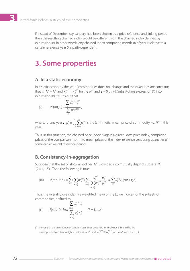
Mixed-form indices: a study of their properties
EURONA — Eurostat Review on National Accounts and Macroeconomic Indicators72
3If instead of December, say, January had been chosen as a price reference and linking period then the resulting chained index would be different from the chained index defined by expression (8). In other words, any chained index comparing month m of year t relative to a certain reference year 0 is path-dependent.
3. Some properties
A. In a static economyIn a static economy the set of commodities does not change and the quantities are constant; that is, τ 0=N N and τ( ) (0)=b b
n nx x for τ∈n N and τ = 0,...,t (9). Substituting expression (1) into expression (8) it turns out that
(9)
(0)
0 (0)( , 0) = ,
mt bn n
c nb
n nn
p xP mt
p x
∑∑
where, for any year τ , 12
1
112
mn n
m
p pτ τ
=
≡ ∑ is the (arithmetic) mean price of commodity τ∈n N in this year.
Thus, in this situation, the chained price index is again a direct Lowe price index, comparing prices of the comparison month to mean prices of the index reference year, using quantities of some earlier weight reference period.
B. Consistency-in-aggregationSuppose that the set of all commodities tN is divided into mutually disjunct subsets t
kN ( =1,..., )k K . Then the following is true:
(10) ( ,0 ; )P mt t b∈ ∈
∈
∑ ∑ ∑ ∑0
00 0
=1
= ( )tb mtK
tb n nn tb t
t tk n nn N n Nk k tn Nk
w pw
w p0
=1
= ( , 0 ; ).K
tbk k
k
w P mt t b∑
Thus, the overall Lowe index is a weighted mean of the Lowe indices for the subsets of commodities, defined as
(11) 0( , 0 ; ) ( =1, ..., ).
mt bn n
tn Nkk t b
n ntn Nk
p x
P mt t b k Kp x
∈
∈
≡∑
∑
(9) Notice that the assumption of constant quantities does neither imply nor is implied by the
assumption of constant weights, that is 0=N Nτ and
( ) (0)=b bn nw wτ
for τ∈n N and τ = 0, ..., .t

Mixed-form indices: a study of their properties
EURONA — Eurostat Review on National Accounts and Macroeconomic Indicators 73
3The weights
(12)
0
0 00
= ( =1, ..., )
t bn n
tn Ntb tb kk n t b
t n nn Nk tn N
p x
w w k Kp x
∈
∈∈
≡∑
∑ ∑
are the mixed-period expenditure shares of the subsets. In other words, the overall Lowe index can be calculated in one stage from the individual commodity price relatives, as in expression (2); or in two stages, as in expression (10): from commodity price relatives to subset Lowe indices and then from these subset indices to the overall index. This is called consistency-in-aggregation (CIA); a very useful property in statistical practice.
Chained indices, however, are not CIA. For such indices, a relation like expression (10) does not exist; in other words, a set of weights (adding up to 1) does not exist, such that
=1
( , 0) = ( , 0),K
c ck k
k
P mt w P mt∑
where ( , 0)ckP mt is the chained price index for subset =1, ...,k K . Only the assumption that the
quantities are constant over the entire time span implies that the chained index exhibits CIA, which does not come as a surprise since any chained Lowe index reduces to a direct Lowe index.
C. Derived measures
MONTHLY CHANGE
The fixed-base nature of a mixed-form index is revealed most clearly when we consider the price change between consecutive months. Thus, the price change between month
−1m and month m of current year t is obtained from the series of chained index numbers ( , 0)cP mτ ( = 0, ..., ; =1, ...,12)t mτ as (10)
(13)
( )
( 1) ( )
( , 0) ( , 0 ; ( ))= = .
(( 1) , 0) (( 1) , 0 ; ( ))
mt b tc n n
nc m t b t
n nn
p xP mt P mt t b t
P m t P m t t b t p x−− −
∑∑
These equalities are obtained respectively by using expression (8) and substituting expression (1). Expression (13) means that the price change between months −1m and m of the same year is measured by a Lowe price index based on quantities of a prior period ( )b t . An important consequence is that if between these two months all the prices change by the same factor, that is, λ −( 1)=mt m t
n np p ( > 0, )tn Nλ ∈ , then the overall price change equals λ (11).
Another consequence is that the overall price change can be written as a weighted arithmetic mean of individual price relatives −( 1)/mt m t
n np p ∈( )tn N .
(10) This is usually presented as a percentage, or a rate of change; that is, ( ( , 0) / (( 1) , 0) 1) 100 %Pc
mt Pc
m t� � � .(11) Put otherwise, ( , 0) / (( 1) , 0)
c cP mt P m t− satisfies the proportionality test.

Mixed-form indices: a study of their properties
EURONA — Eurostat Review on National Accounts and Macroeconomic Indicators74
3ANNUAL CHANGE
We now look at the price change between corresponding months of consecutive years; that is, τ τ −( ,0) / ( ( 1),0)c cP m P m τ( =1,..., ; =1,...,12)t m .Employing expression (8), the price change between months m of years −1t and t is measured as
(14) ( , 0) ( , 0 ; ( )) (12( 1), 0( 1); ( 1))
= .( ( 1), 0) ( ( 1), 0( 1); ( 1))
c
c
P mt P mt t b t P t t b t
P m t P m t t b t
− − −− − − −
By substituting expression (1) we obtain
(15)
− −
− −×−
∑ ∑∑ ∑
( ) 12( 1) ( 1)
0 ( ) ( 1) ( 1)
( ,0)= .
( ( 1),0)
mt b t t b tc n n n n
n nc t b t m t b t
n n n nn n
p x p xP mt
P m t p x p x
The annual price change appears to be the product of two Lowe price indices, each having their own set of quantity weights: the first index compares prices of month m of year t to December of year −1t , and the second index compares prices of December of year −1t to month m of year −1t . The first index is based on the commodity set tN and the second on commodity set −1tN .
If these commodity sets are the same, then expression (15) can be rewritten as
(16)
( ) 0 ( 1)
( 1) ( 1) 0 ( )
( , 0)= ,
( ( 1), 0)
mt b t t b tc n n n n
n nc m t b t t b t
n n n nn n
p x p xP mt
P m t p x p x
−
− − ×−
∑ ∑∑ ∑
where use was made of the fact that −12( 1) 0=t tn np p for all −∈ 1 =t tn N N . The right-hand side
of expression (16) has the form of a value index divided by a quantity index. It is a so-called implicit price index, but not a genuine price index: if in the corresponding months m all the later prices happen to be the same multiple of the former prices, that is, λ −( 1)=mt m t
n np p λ −∈ 1( > 0, = )t tn N N , then the annual price change does not necessarily equal λ . In other
words, the annual price change cannot be written as a weighted mean of the individual price relatives −( 1)/mt m t
n np p .
Nevertheless, it is possible to decompose the annual price change into contributions of the individual commodities and/or contributions of the current and the previous year. The solution suggested by Ribe (1999) amounts to rewriting expression (15) as
(17)
( ) 12( 1) ( 1)
0 ( ) ( 1) ( 1)
( , 0)1= 1
( ( 1), 0)
mt b t t b tc n n n n
n nc t b t m t b t
n n n nn n
p x p xP mt
P m t p x p x
− −
− −
− − × −
∑ ∑∑ ∑
12( 1) ( 1)
( 1) ( 1)1 .
t b tn n
nm t b tn n
n
p x
p x
− −
− −
+ −
∑∑
However, by looking at the structure of the right-hand side it becomes clear that this decomposition is not completely satisfactory. Though the second factor in brackets can be interpreted as previous year’s contribution, and the first factor in brackets likewise as current year’s contribution (and both factors can be decomposed commodity-wise), this first factor is multiplied by previous year’s price change. Thus, there seems to be a trace of double-counting here.

Mixed-form indices: a study of their properties
EURONA — Eurostat Review on National Accounts and Macroeconomic Indicators 75
3A different solution, involving logarithmic means (12), was proposed by Balk (2006). Consider the first factor at the right-hand side of expression (15) and use the logarithmic mean and its linear homogeneity (that is, property (3)) to obtain the following decomposition:
(18) ∈
−
∑∑∑
( )0
0 ( ) 0ln = ,
mt b tmt tn n
mt n nnnt b t t
tn n nn Nn
p xp p
wp x p
where the weights are defined as
0 ( )
0 ( )
1( ).
( ( , 0 ; ( )),1)
t b tmt tn nn t b t
n nn
p xw n N
LM P mt t b t p x≡ ∈
∑
Similarly, decomposing the second factor delivers
(19)
− −− −
−− − −
−∈
−
∑∑∑
12( 1) ( 1)12( 1) ( 1)
( 1)( 1) ( 1) ( 1)
1
ln = ,
t b tt m tn n
m t n nnnm t b t m t
tn n nn Nn
p xp p
wp x p
where the weights are defined as
( 1) ( 1)( 1) 1
( 1) ( 1)
1( ).
( (12( 1), ( 1); ( 1)),1)
m t b tm t tn nn m t b t
n nn
p xw n N
LM P t m t b t p x
− −− −
− −≡ ∈− − − ∑
By combining the two factors it appears that the annual price change can be decomposed as follows:
(20) 0 12( 1) ( 1)
( 1)0 ( 1)
1
( , 0)ln = .
( ( 1), 0)
c mt t t m tmt m tn n n nn nc t m t
t tn nn N n N
P mt p p p pw w
P m t p p
− −−
−−∈ ∈
− −+ −
∑ ∑
Since for any positive real number ≠1a , ln = ( 1) / ( ,1)a a LM a− , the left-hand side of expression (20) is a simple transformation of the inflation rate. In fact, for ≈1a , the usual approximation is ≈ −ln 1a a . The right-hand side of the expression then provides a decomposition of the inflation rate into contributions of the individual commodities, divided with respect to current year t and previous year −1t . The commodities can be grouped into those available in both years, those available in the current year but not in the previous year, and those available in the previous year but not in the current year.
(12) For any two positive real numbers a and b, their logarithmic mean is defined by ( , ) ( ) / ln( / )LM a b a b a b≡ − when ≠a b, and ( , ) .LM a a a≡ It has the following
properties: (1) min( , ) ( , ) max( , );a b LM a b a b≤ ≤ (2) ( , )LM a b is continuous;
(3) ( , ) = ( , )LM a b LM a bλ λ λ λ( >0); (4) ( , ) = ( , )LM a b LM b a ; (5) 1/2
( ) ( , ) ( ) / 2;ab LM a b a b≤ ≤ +
(6) ( , 1)LM a is concave. More details in Balk (2008, pp. 134-136).

Mixed-form indices: a study of their properties
EURONA — Eurostat Review on National Accounts and Macroeconomic Indicators76
3MEAN ANNUAL CHANGE
The annual price change, obtained by comparing the same month of two adjacent years, will generally remove any regularly occurring seasonal variation. To provide a statistic that is robust to both regular and irregular (seasonal) variations, a 12-months moving average of annual price changes is frequently used.
We will consider here in particular the moving average as obtained in December of any year; that is, the mean of ratios
(21) 12
=1
1 ( , 0),
12 ( ( 1), 0)
c
cm
P mt
P m t −∑and compare this with the ratio of mean indices
(22)
12
=112
=1
1( , 0)
12 .1
( ( 1), 0)12
c
m
c
m
P mt
P m t −
∑
∑The last ratio can be given a solid interpretation. To see this, we substitute expression (8) into expression (22). Cancelling common factors in numerator and denominator, we obtain
(23)
12
=112
=1
1( , 0)
12 =1
( ( 1), 0)12
c
m
c
m
P mt
P m t −
∑
∑
12
=112
=1
1( , 0 ; ( ))
12 (12( 1), 0( 1); ( 1)),1
( ( 1), 0( 1); ( 1))12
m
m
P mt t b tP t t b t
P m t t b t− − −
− − −
∑
∑
which after substituting expression (1) thrice becomes
(24)
12
=112
=1
1( , 0)
12 =1
( ( 1), 0)12
c
m
c
m
P mt
P m t −
∑
∑
( )12
0 ( ) 12( 1) ( 1)=1
( 1) ( 1) 0( 1) ( 1)12
0( 1) ( 1)=1
112
=
112
mt b tn n
nt b t t b t
m n n n nn n
m t b t t b tn n n n
n nt b t
m n nn
p x
p x p x
p x p x
p x
− −
− − − −
− −
∑∑ ∑ ∑∑ ∑
∑ ∑
( ) 0 ( 1)
1 ( 1) 0 ( ),
t b t t b tn n n n
n nt b t t b tn n n n
n n
p x p x
p x p x
−
− −
∑ ∑∑ ∑
where 12
1
112
mn n
m
p pτ τ
=
≡ ∑ τ∈( )n N are annual mean prices and it is useful to recall that month 12
of year −1t is the same as month 0 of year t . The final part of expression (24) contains two components. The left factor is a (counterfactual) value index comparing weight reference period ( )b t quantities at mean period t prices to weight reference period −( 1)b t quantities at mean period −1t prices. The right factor is the reciprocal of a (Lowe) quantity index comparing weight reference period ( )b t quantities to those of weight reference period
−( 1)b t . If −( ) = ( 1)b t b t then this factor vanishes.
Summarising, the ratio of annual mean indices in expression (22) may be interpreted as an implicit price index for year t relative to year −1t . If −( ) = ( 1)b t b t then this implicit price index reduces to a Lowe price index.

Mixed-form indices: a study of their properties
EURONA — Eurostat Review on National Accounts and Macroeconomic Indicators 77
3To relate now the mean of annual ratios, expression (21), to the ratio of annual means, expression (22), we proceed as follows. Employing the logarithmic mean, the logarithm of the ratio of annual means can be decomposed as
(25)
12
12=1
12=1
=1
1( , 0)
( , 0)12ln = ln ,1 ( ( 1), 0)( ( 1), 0)
12
cc
mmc
c m
m
P mtP mt
P m tP m t
Ψ − −
∑∑
∑
with
12 12
=1 =1
12
12 12=1
=1 =1
( , 0) ( ( 1), 0),
1 1( , 0) ( ( 1), 0)
12 12( =1, ...,12).
( , 0) ( ( 1), 0),
1 1( , 0) ( ( 1), 0)
12 12
c c
c c
m m m
c c
c cm
m m
P mt P m tLM
P mt P m tm
P mt P m tLM
P mt P m t
− − Ψ ≡ − −
∑ ∑
∑∑ ∑
The weights Ψm are the normalised, mean-over-two-years ratios of monthly price index to annual mean price index, and as such reflect the aggregate seasonal price level pattern.
Now return to the mean of annual ratios in expression (21). Being an arithmetic mean it is greater than or equal to a geometric mean. Thus,
(26) 12 12
=1 =1
1 ( , 0) 1 ( , 0)ln ln =
12 ( ( 1), 0) 12 ( ( 1), 0)
c c
c cm m
P mt P mt
P m t P m t
≥ − −
∑ ∑
12 12
=1 =1
( , 0) 1 ( , 0)ln ln =
( ( 1), 0) 12 ( ( 1), 0)
c cm m
c cm m
P mt P mt
P m t P m t
Ψ − Ψ − − − ∑ ∑
12
12=1
12=1
=1
1( , 0)
1 ( , 0)12ln ln ,1 12 ( ( 1), 0)( ( 1), 0)
12
cc
mmc
c m
m
P mtP mt
P m tP m t
− Ψ − − −
∑∑
∑
where at the last step expression (25) has been used. The term after the minus sign in expression (26) measures the covariance between seasonal price level, as measured by the Ψm , and monthly measured annual price change (between consecutive years),
( , 0) / ( ( 1), 0)c cP mt P m t − . As the latter does not contain any (regular) seasonal pattern, we expect the covariance to be zero. The implication is that the mean of ratios is greater than the ratio of means and, in view of the interpretation of the latter as provided by expression (24), can be said to overstate mean annual price change.

Mixed-form indices: a study of their properties
EURONA — Eurostat Review on National Accounts and Macroeconomic Indicators78
3
4. ConclusionA traditional distinction runs between direct and chained indices. Mixed-form indices share features of these two kinds: in the short run they behave as direct indices, and in the long run as chained indices.
Mixed-form indices usually materialise when monthly indices have to be compiled, typical examples being the HICP and CPIs compiled by national statistical offices. Their mixed form is revealed most clearly when derived measures such as monthly or annual rates of change are considered; the interpretation of these requires some care.
AcknowledgementsThe author would like to thank Jens Mehrhoff, Robert O’Neill and two anonymous referees for their careful reading and constructive comments.
ReferencesBalk, B. M. (2006), ‘Measuring and Decomposing Rates of Inflation Derived from Annually Chained Lowe Indices’, paper presented at the 9th meeting of the Ottawa Group on price indices, 14-16 May 2006, London, available at: www.ottawagroup.org.
Balk, B. M. (2008), Price and Quantity Index Numbers: Models for Measuring Aggregate Change and Difference, Cambridge University Press, New York.
Balk, B. M. (2010), ‘Direct and Chained Indices: A Review of Two Paradigms’, in Price and Productivity Measurement: Vol. 6 — Index Number Theory, edited by Diewert W. E., B. M. Balk, D. Fixler, K. J. Fox and A. O. Nakamura, Trafford Press, available at: www.vancouvervolumes.com and www.indexmeasures.com.
International Labour Office, International Monetary Fund, Organisation for Economic Co-operation and Development, Statistical Office of the European Community, United Nations and World Bank (2004), Consumer price index manual: Theory and practice, International Labour Office, Geneva.
Ribe, M. (1999), Effects of Subcomponents on Chained Price Indices Like the HICPs and the MUICP, mimeo dated 23 September 1999, Statistics Sweden.
von der Lippe, P. (2001), ‘Chain Indices; A Study in Price Index Theory’, Vol. 16, Spectrum of Federal Statistics, Statistisches Bundesamt, Wiesbaden.
von der Lippe, P. (2007), Index Theory and Price Statistics, Peter Lang GmbH, Frankfurt am Main.
4 Dynamic pricing as a challenge for consumer price statistics (1)CHRISTIAN BLAUDOW, FLORIAN BURG (2)
Abstract: the use of automated algorithms allows online shops to change product prices at short notice, depending on various parameters; this type of price-setting is known as dynamic pricing. At present, roughly 10 000 online prices are collected each month by the German Federal Statistical Office (FSO) for the German consumer price index (CPI) and the harmonised index of consumer prices (HICP), but in many cases only one price is observed each month for each product, usually at a given point in time. Dynamic pricing poses a potential challenge to consumer price statistics: to capture the correct monthly average price and to process volatile prices. To understand this challenge, a study on dynamic pricing was conducted in 2017. It was limited to products and online shops that were included in the CPI/HICP sample and used web scraping to collect prices.
Keywords: consumer price index, harmonised index of consumer prices, dynamic pricing, online price collection, web scraping.
(1) This paper has been presented at a meeting of the Ottawa Group on 10-12 May 2017 in Eltville am Rhein (Germany) and was updated in March 2018.
(2) Destatis — the Federal Statistical Office of Germany.

Dynamic pricing as a challenge for consumer price statistics
EURONA — Eurostat Review on National Accounts and Macroeconomic Indicators80
4
1. Introduction
A. What is dynamic pricing?In general, dynamic pricing is the use of automatic algorithms to change prices at short notice due to changes in market conditions or due to parameters indicating a consumer’s willingness to pay.
The phenomenon that prices change rapidly depending on market conditions is of course not new. Prior to the widespread use of e-commerce this was limited to goods and services for which price changes could be announced at little or no cost. For automotive fuels, for instance, prices could be changed several times a day, supported by the use of electronic price signs on the forecourts of petrol stations. Prices also used to change at relatively short intervals for some transport and travel services, such as flights, package holidays or rental cars. Their price strongly depends on the time of booking as well on the time when the service is provided. In the past, booking was mainly done through travel agencies, but nowadays this is done to a large extent using the internet. This development allows for immediate price adjustment due to factors like capacity, or calendar effects such as weekend or Christmas business. To take account of these price changes, price collectors for the German CPI/HICP collect prices several times each month according to a fixed schedule. However, this is time consuming and restricted by staff resources and hence, for some selected products, prices are collected using web scraping techniques.
Besides these special categories of goods and services, dynamic pricing would appear to be a practice of growing importance. Firstly, the phenomenon of dynamic pricing is present in (at least) the German media (Jung (2017); Fischer et al. (2017); Klemm (2017); Hoffmann (2018)). However, the incidence of dynamic pricing and the extent of its use in online markets have not yet been profoundly investigated in scientific literature. Secondly, a market has developed for tools to optimise prices displayed on online websites. Retailers who offer goods and services on websites have the potential to make immediate price changes in order to react to changing market conditions. Major online traders employ their own specialists for optimising their online pricing policy. There are also tools which can be used to observe product prices in online shops and inform small businesses and/or consumers when the price of a certain product falls below a pre-defined threshold. Indeed, the number of online price comparison portals and online price monitoring tools such as Minderest, Patagona, Price2spy and the IBM dynamic pricing tool has increased steadily in recent years. These developments suggest that the phenomenon of dynamic pricing plays an increasing role for online traders and for consumers.
Looking at this phenomenon from the perspective of price statisticians, dynamic pricing makes it more difficult to measure the price developments of products in online shops and — as the online market seems to have gained importance in recent years — leads to new challenges when compiling consumer price indices. Therefore, one of the fundamental

Dynamic pricing as a challenge for consumer price statistics
EURONA — Eurostat Review on National Accounts and Macroeconomic Indicators 81
4questions dealt with in this paper concerns the extent of dynamic pricing. How large and how common is this issue nowadays? For this reason, the goal of the present study was to investigate the frequency and level of price changes of products that are relevant for the compilation of the German CPI/HICP.
Various shops in Germany have recently introduced digital price signs, at least on an experimental basis. If the share of digital price signs further increases, dynamic pricing will not only be an issue for price collection from online shops, but also for price collection in physical (so-called ‘bricks and mortar’) shops. One solution to capture dynamic pricing that is applied in physical shops is to use transaction data (scanner data). Transaction data record the transactions of actual events when consumers buy goods or services. This is a promising, but also challenging approach which is not discussed in this paper. Furthermore, this study is not concerned with the collection of individualised pricing, namely, the practice of offering different prices to different consumers at different times (Schleusener (2016); Remmel (2016)). In particular, individualised pricing describes the phenomenon of trying to charge every customer the individual price that he/she is willing to pay for a certain good based on the (individual) value he/she places on the product at the moment of purchase. This paper deals solely with dynamic pricing and an analysis of dynamic price changes over time.
B. Price collection using the internet for the German CPI/HICPThe basket of goods and services used for the German consumer price statistics contains at its upper level approximately 600 different types of goods and services (Egner (2013)). For the vast majority of these goods and services, a traditional price collection exercise is conducted at physical shops and service providers: a total of more than 300 000 individual price observations are made each month. This traditional price collection is usually conducted at one point during the month, in other words, usually only one price observation is made each month for each product and this is then used for the calculation of average prices which in turn are further used for the calculation of sub-indices up to the overall CPI/HICP. In addition to this traditional price collection, prices are collected for certain goods and especially services that require a more sophisticated survey design (for example, the price of flights or package holidays).
For online shops, the price collection is conducted centrally by the FSO for efficiency reasons. For the majority of goods sold this way, prices are collected manually at one point in time during the month. For the German CPI, weights for different shop types at the level of products were introduced in 2008 (Sandhop (2012)). The overall weight of online shops in all shop types was approximately 5 % for the base year 2010, which is expected to increase in the coming years.
Although the online market is expected to expand further, it is important to note that a much larger amount of prices still refer to goods and services not offered online — or at least they are not offered exclusively online — and that they are therefore not subject to dynamic pricing.

Dynamic pricing as a challenge for consumer price statistics
EURONA — Eurostat Review on National Accounts and Macroeconomic Indicators82
4
2. Set-up of the study
A. Sample designThe sample of products for the present study consists exclusively of products offered by online shops which are observed for the regular monthly price collection for CPI/HICP. These products and online shops are specified by the CPI/HICP framework, with every product in the sample assigned to a COICOP-10-digit heading (3). The sample was composed solely of goods (no services) covering 242 COICOP headings. At the beginning of the study, the sample started with 3 050 products, distributed across 15 online shops: online shops with a relatively large number of price observations and known to have a large market share were selected for the study. As a result of data collection issues (non-availability of products, explained below), the final analysis was based on 2 680 products and 14 online shops. The prices were collected using web scraping techniques. Since a couple of years ago, these techniques have been used by the German FSO for automatically collecting prices from the internet, and an increasing number of national statistical offices make use of these techniques for their online price collection (Griffioen et al. (2014); Nygaard (2015)).
The target of the present study was to investigate the frequency of price changes of products relevant for the German CPI/HICP for a group of online retailers. The automatic collection of price observations was carried out with an hourly rhythm, allowing many price observations to be made. Consequently, a detailed picture emerged of price developments in online shops and the study was able to investigate the incidence of dynamic pricing and the extent of daily and hourly price changes.
B. Technical instruments and procedure for the data collection program (4)The sample’s product input data including product name, shop, COICOP number, COICOP name, unique identifier, product URL (5) and product’s article number was uploaded to an input table of a relational database. In order to access each product’s offer page directly, it was essential to find the URL for each specific product. Another input table was created which included the XPaths (6) of the offer pages for the respective online shops. As such, XPaths for the position of the product name, normal price, special price, article number and product availability were stored only once for each shop. Earlier studies have shown that the use of XPaths instead of using HTML-elements for the extraction of information is the most stable solution.
(3) COICOP: classification of individual consumption of purpose. COICOP-10-digit is the lowest (most detailed) level of the classification used for German consumer price statistics and represents the elementary product groups that form the basis for the price collection exercise for CPIs/HICPs.
(4) For further explanations, see Blaudow (2018).(5) Uniform resource locator (reference to a web resource).(6) XPath is a syntax for defining parts of an XML document; it can be used to navigate through
elements and attributes in an XML document.

Dynamic pricing as a challenge for consumer price statistics
EURONA — Eurostat Review on National Accounts and Macroeconomic Indicators 83
4The procedure for automated price collection was programmed in Java (see Figure 4.1). The web scraping was carried out using a tool called Selenium that controls a web browser; this tool may be installed as a plug-in for a common internet browser and can then be used for recording and replaying procedures within a browser. Additionally, Selenium offers programming interfaces in various languages including Java. Once implemented, the browser is then used to execute the scraping processes as well as to find the relevant positions of information. Selenium only functions as a provider of information and an interface between Java and the browser. The use of an internet browser for retrieving the information from a webpage is very efficient and flawless and had additional advantages. For instance, when using a common internet browser, it is possible to disable scripts (7) on a page and to start and shut down a browser window within a short amount of time. Additionally, browser windows operate completely independently from each other. Therefore, it is possible to run several browser windows for price collection simultaneously. These advantages lead to a huge increase in speed of price collection.
Figure 4.1: Technical set-up
In addition, the project used steadily changing IP addresses. Therefore, the influence of individual consumer behaviour on the price of the product could not be observed. The prices shown on the page are definitely the prices of the shops for any customer and are not individualised prices. It should be noted that this study was not able to investigate the influence of different electronic devices for the price collection since the prices were collected with the same electronic device.
(7) Online shops use different types of scripts, JavaScript foremost, to adjust features on their webpages easily or simply to enable interactive webpages. There are scripts which complicate the extraction of information but in some cases also give additional or even necessary information. In general, the developers of the program tried to disable (forbid) as many scripts as possible to ensure that the process of price extraction ran without any delay due to page loading.
Input Output

Dynamic pricing as a challenge for consumer price statistics
EURONA — Eurostat Review on National Accounts and Macroeconomic Indicators84
4C. Treatment of data gapsThe automated price collection exercise started on 9 December 2016 and lasted until 6 March 2017 in order to have data for almost three months. The main part of the study included an analysis of the frequency of price changes and the volatility of price developments. Originally, the program was supposed to collect prices for a whole year. Unfortunately, over the course of the year, a large number of prices failed to be collected due to non-availability of the products. In order to evaluate a comparable sample after a period of one year, these products which were no longer available would have had to be replaced in a short time, as done for manual price collection. Replacements were not sought, as within the concepts of consumer price statistics they should not be automated at all (or at least not without insightful algorithms, which was not possible within the limits of this study). As a result, if products were not found for a certain period of time, the product was removed from the analysis. For this reason, the evaluation period was shortened to three months for the whole sample of products, as comparability would have been poor if online shops with a large proportion of failed products were included in the analysis alongside online shops with relatively few products that could not be found.
Due to the large number of products and the long time period of the data collection, some gaps in the series of prices occurred. The vast majority of these gaps were caused by technical problems. Therefore, the following post-processing was carried out:
• As long as data gaps were assessed to be temporary (in other words, a price could be scraped again after a certain period of time), imputation was done to have complete series of prices. In most cases, an unsuccessful extraction of a product’s price was caused by a temporary shutdown of the online shop’s webpages due to maintenance. In such cases, the last price found for the product was used to fill the gaps. Several shops use ‘maintenance procedures’ on their websites in order to make general price changes for their products. For this reason, when looking at the time of price changes of every single shop, there is often a cluster of price changes during the night (see Figure 4.3).
• Only price series with at least 50 % of the possible number of price observations were taken into account. Products which had not been observed for at least half of the investigation period were deleted prior to the analysis.
• A manual check was done for products with price increases of at least 500 % as well as for products which experienced excessive price decreases of more than 80 %. In most of these cases, replacements occurred and, in a few cases, the article number of the old product was used for a new product. This was also the case for some products which were removed by an online shop, with customers being redirected to a new webpage that detailed a similar (but not the same) product. These series were not taken into account in the analysis as the products were not identical, even if they were similar from the online shop’s point of view.
• One online shop closed down approximately two months after starting the automated price collection exercise. Since this shop was no longer relevant for the price collection of the CPI/HICP, its historical prices were also excluded from the analysis.
After these data cleansing processes had been applied, 2 680 price series for products in 14 online shops remained in the data set and formed the basis for the analysis. The results presented here for this one-off exercise are anonymised. This anonymisation is not crucial for the analysis. For regular price collection, however, it is very important to know in which shops dynamic pricing is conducted in order to be able to introduce more frequent survey intervals and additional checks at the end of each month.

Dynamic pricing as a challenge for consumer price statistics
EURONA — Eurostat Review on National Accounts and Macroeconomic Indicators 85
4
3. ResultsThis chapter deals with the most important results of the study. At first, the number of price changes for the whole sample is evaluated. Secondly, we compare the online shops with respect to the number of price changes for each product and then continue to assess the volatility of the price changes of these products. The chapter ends with an analysis of the time when price changes are made.
A. Number of price changes during the observed periodWe will first look at the number of price changes for each product during the observation period, split into four categories. From the perspective of consumer price statistics, it is valuable to know how many products change their prices in a way that the manual price collection is not able to capture. The following figure shows the results:
Figure 4.2: Share of products by number of price changes during the observation period
The first two categories — either no price change or one to three price changes during the three-month period of the study — were chosen as (assuming evenly spread price changes) they reflect a similar number of price changes that might be captured if using manual price collection conducted at one point in time during the month.
In general, the unit value price over the entire month is the target price to be collected. If the price changes on average more than once each month, the traditional methods for price collection could perhaps lead to the inclusion of less representative prices (outliers) compared with the unit value; when performing the index calculation the price collector and the index compiler do not know whether the single observed price is representative.
Almost one quarter of the sample was made up of products where the price changed 4-15 times during the course of the study. This frequency of price changes is not entirely captured by the current manual price collection techniques. With a price collection once each month
No price changes43.0 %
1-3 price changes22.1 %
4-15 price changes23.1 %
> 15 price changes11.7 %

Dynamic pricing as a challenge for consumer price statistics
EURONA — Eurostat Review on National Accounts and Macroeconomic Indicators86
4there is a growing risk that the observed price is not representative for the monthly average price of a particular product. A relatively small share of products in the sample (11.7 %) changed price more than 15 times during the observation period; this means that on average they had more than five price changes each month. In general, the higher the number of price changes for each product each month, the more unlikely it is that the current manual price collection is able to observe a representative price for the respective month. Moreover, it is also important to consider the variation of the respective price changes (as we will see in the following section).
Table 4.1 compares online shops with respect to the frequency with which they changed their prices for various products. It shows that the share of products with no price changes or with 1-3 price changes was significantly higher for a majority of online shops (shops 2, 3, 5, 7, 8, 10, 11, 12 and 13) than for the remaining shops. These results indicate that dynamic pricing is only broadly applied by some online shops, whereas for other online shops the frequency of price changes seem to be in a range that is usually captured by the current manual price collection and is not caused by special techniques of dynamic pricing.
Table 4.1: Number and share of price series analysed by the frequency of price changes during the observation period, by online shop
Online shop
Price changes0 1-3 4-15 >15
Total number of price series
(number of price series)
(%)(number of price series)
(%)(number of price series)
(%)(number of price series)
(%)
Shop 1 17 7.91 20 9.30 76 35.35 102 47.44 215
Shop 2 268 47.94 109 19.50 114 20.39 68 12.16 559
Shop 3 105 50.72 54 26.09 44 21.26 4 1.93 207
Shop 4 15 20.55 13 17.81 34 46.58 11 15.07 73
Shop 5 19 32.76 37 63.79 2 3.45 0 0.00 58
Shop 6 21 25.61 21 25.61 30 36.59 10 12.20 82
Shop 7 483 54.39 174 19.59 145 16.33 86 9.68 888
Shop 8 21 84.00 4 16.00 0 0.00 0 0.00 25
Shop 9 6 4.88 36 29.27 60 48.78 21 17.07 123
Shop 10 23 31.51 19 26.03 31 42.47 0 0.00 73
Shop 11 16 29.63 19 35.19 15 27.78 4 7.41 54
Shop 12 59 79.73 11 14.86 1 1.35 3 4.05 74
Shop 13 75 68.81 33 30.28 1 0.92 0 0.00 109
Shop 14 25 17.86 43 30.71 67 47.86 5 3.57 140
Total 1 153 43.02 593 22.13 620 23.13 314 11.72 2 680

Dynamic pricing as a challenge for consumer price statistics
EURONA — Eurostat Review on National Accounts and Macroeconomic Indicators 87
4B. Volatility of pricesThe following analysis is restricted to only those cases in which the price of a product changed more than three times during the observation period; this subset is used to analyse the volatility of prices (see Table 4.2). To measure the volatility of prices, the coefficient of variation was calculated for each price series. The coefficient of variation is a measure of dispersion and was chosen because it is a relative measure that does not depend on the absolute level of prices.
The analysis has an important impact on the assessment of the current way of collecting prices manually. When the volatility of prices is low, dynamic pricing might not be a major problem for measuring inflation (in other words, for the calculation of the CPI/HICP). For example, more than four fifths of the observed products offered by Shop 1 saw their price change at least four times during the observation period (in other words more than once each month on average), while the price of almost half the products sold by online Shop 1 changed more than 15 times (more than 5 times each month on average). By contrast, the coefficient of variation for more than four fifths of the observed products offered by Shop 1 was below 0.1 and was even below 0.05 for 55 % of the observed products. This indicates that dynamic pricing was applied in Shop 1, but that the volatility of prices is in a range that could be captured by an extension of the number of points in time of the current manual price collection method. When the fluctuation in the price of a product has a low coefficient of variation, it is unlikely that an incorrect measurement of the monthly price development will occur when using current methods, as it is unlikely that one observed price is an extreme price for the product in question. For instance, one of the observed products offered by Shop 1 changed its price 1 304 times during the three-month period of the study with a coefficient of variation of just 0.02.
Across all online shops in the sample the coefficient of variation for prices was below 0.1 for two thirds (66 %) of the price series where the price changed more than three times during the three month period of the study, while for 42 % of these price series the coefficient of variation was below 0.05.
By contrast, there are also cases for which the price of a product changed almost every hour and did so with a high coefficient of variation. Two examples are shown in the appendix (see Figure 4.4 and Figure 4.5). Without the use of modern techniques such as web scraping, frequent price changes as shown in both of these figures are impossible to capture. Considering the two examples, seasonality is not apparent and the range of price changes is not explainable.
There were only a few online shops for which a relatively high number of price changes was observed with a relatively high coefficient of variation. For example, in Shop 14, prices changed frequently (see Table 4.1) and with a relatively high coefficient of variation (see Table 4.2).

Dynamic pricing as a challenge for consumer price statistics
EURONA — Eurostat Review on National Accounts and Macroeconomic Indicators88
4Table 4.2: Number of price series for which more than three price changes were recorded during the observation period, by online shop and coefficient of variation
Online shopCoefficient of variation
<0.05 0.05-<0.1 0.1-0.25 >0.25Shop 1 99 46 27 6
Shop 2 67 44 52 19
Shop 3 26 19 2 1
Shop 4 38 7 0 0
Shop 5 0 0 0 2
Shop 6 24 13 3 0
Shop 7 75 40 67 49
Shop 8 0 0 0 0
Shop 9 47 24 9 1
Shop 10 2 18 11 0
Shop 11 11 5 3 0
Shop 12 0 1 1 2
Shop 13 0 0 1 0
Shop 14 5 6 57 4
Total 394 223 233 84
C. Time of price changesLooking at the time of day when price changes occurred (see Figure 4.3), there was a clear pattern with many price changes taking place during the first third of the day, especially between midnight and 1 a.m. This is probably caused by technical reasons: for example, some (more simple) tools used for dynamic pricing only allow price changes once a day; online shops may try to change their prices at a time when there are less consumers shopping online. By contrast, during those periods when most consumers are shopping — the afternoon and evening — it seems clear that online shops avoid changing prices as this is assumed to annoy and/or discourage consumers (Remmel (2016)).
Figure 4.3: Average number of price changes during the observation period, by hour(number)
0
500
1 000
1 500
2 000
2 500
3 000
3 500
0:00
1:00
2:00
3:00
4:00
5:00
6:00
7:00
8:00
9:00
10:0
0
11:0
0
12:0
0
13:0
0
14:0
0
15:0
0
16:0
0
17:0
0
18:0
0
19:0
0
20:0
0
21:0
0
22:0
0
23:0
0
Hour
Dynamic pricing as a challenge for consumer price statistics
EURONA — Eurostat Review on National Accounts and Macroeconomic Indicators 89
4
4. Implications for consumer price statisticsThe information presented in this study about online shops and their price setting behaviour with respect to the frequency of price changes and the volatility of price series is very important for price collectors and price index compilers. With this information, resources for price collection can be managed in a different way, assigning more resources to the collection of prices from online shops which display a high frequency of price changes and a high volatility of prices. Certainly, price setting behaviour has to be monitored on a regular basis which may be done with the help of web scraping.
Applying the results of this study to consumer price statistics provides the following insights:
• There is evidence that at the moment dynamic pricing is only applied to a large extent by relatively few online shops. Dealing with this is a major task to tackle in the near future with improved methods and tools. Web scraping which was used in the present study is a suitable tool to improve the current monthly price collection methods.
• The study has revealed that for two thirds of the products surveyed, the price did not change more than three times during the observation period covering almost three months. Assuming that these price changes are evenly spread over time (in other words, no more than one change in price each month) these price changes are captured by the current manual price collection methods for consumer price statistics (one price observation each month). For the remaining one third of products in the sample, consumer price statistics will have to find ways to collect prices more frequently.
• For the products identified as having 4-15 price changes during the three month period, more frequent manual price collection and additional checks could be an acceptable solution. For the products where prices changed more than 15 times during the three month period, web scraping provides a suitable tool for price collection.
• The frequency with which prices change is not of major concern for the calculation of consumer price indices as long as the coefficient of variation remains below a certain level. Considering products for which the price changed more than three times during the three month period (an average of more than once each month) and where simultaneously the coefficient of variation was more than 0.05, to be not manageable by the means of current manual price collection methods, leads to the outcome that 20 % of the observed prices in this study may lead to an incorrect measurement of the monthly price development.
• Finally, the timing (during the day) of the price changes has to be considered as well. Manual price collection should preferably take place during periods when consumers typically make their purchases, assuming that during those periods the prices are more representative as they tend to be relatively stable. However, this assumption has to be proved through a more in-depth analysis than has done so far.
Moreover, it has to be mentioned that the extension of automated price collection may also pose methodological challenges to statisticians. Replacement products and the corresponding quality adjustments will likely be difficult to automate, especially for technical products. Following the traditional bilateral approach of comparing single products over time,

Dynamic pricing as a challenge for consumer price statistics
EURONA — Eurostat Review on National Accounts and Macroeconomic Indicators90
4replacement products and quality adjustments will likely remain a task for price collectors/product experts. An alternative approach would be the use of multilateral methods, which are not discussed in this paper. Nevertheless, in the near future, the majority of the workload of a price collector will cover the task of plausibility checking, the implementation of replacement products and quality adjustments rather than the actual collection of price data.
Moreover, calculating average prices based on prices scraped at regular intervals (for example, every hour as in the present study) is straightforward only at first sight. It is questionable whether all scraped prices are representative and therefore suitable for the calculation of price indices (Mayhew (2017); Breton et al. (2016); Cavallo (2018)). Indeed, consumers may face prices at a level at which a purchase is unlikely. Against this background, calculating average prices over time based on scraped prices requires the elimination of such outliers and the imputation of missing prices. One possible approach to solve the problem of detecting unusual price quotes is to use transaction data. By doing so, there is no need to calculate average prices or to collect more prices (in case of products with volatile prices). More precisely, only prices of products which actually formed the basis for a purchase by a consumer would enter into the average price calculation; in this case, a complex method of outlier recognition is not necessary.
5. Conclusions and outlookThe main result of the study presented in this paper is that dynamic pricing is in fact currently applied in some online shops. One may draw the conclusion that only larger online retailers can afford the application of complex and high-capacity algorithms. This result can be interpreted positively: it makes it possible to concentrate on the application of new tools (like web scraping) and the introduction of more frequent manual price collection and checks for certain online shops which have a high frequency of price changes and a high volatility of price series. For online shops with low numbers of price changes and low volatility of price series, the current manual price collection method seems to be sufficient.
The use of web scraping presents an efficient way of conducting price collection using the internet in the future, since fewer resources are needed in the medium-term to set up these techniques in comparison with collecting prices manually. However, the extension of automated price collection also poses methodological challenges to statisticians. Replacement products and the corresponding quality adjustments will likely be difficult to automate, especially for technical products.

Dynamic pricing as a challenge for consumer price statistics
EURONA — Eurostat Review on National Accounts and Macroeconomic Indicators 91
4There are numerous aspects worth analysing in more detail in future studies. These include, for instance, the incidence of individualised pricing. In order to analyse this particular phenomenon, it is necessary to create different designs for automated price collection. Exemplary designs may be the use of different devices that may be used when navigating to online shops or the inclusion of different consumption patterns indicated by the pages visited before making a purchase (8). Furthermore, a long-term analysis of online prices collected through manual price collection methods compared with online prices collected using web scraping seems an obvious and instructive area to explore. For this reason, the German FSO is currently working on the implementation of a similar survey, including 10 000 products at roughly 400 online shops. Prices will be collected hourly for an observation period of 12 months and then analysed. The actual price collection will again be performed using web scraping techniques. But this time, where possible, manual and automated replacements will be put in practice for cases where a product disappears. In the end, this long-term analysis will make possible a comparison between online prices collected by manual price collection methods and online prices collected using web scraping.
To sum up, on the basis of the present study, dynamic pricing is an issue to be tackled in the coming years. However, from the perspective of consumer price statistics, two out of three price developments are still captured using traditional price collection methods, while the remaining price developments will have to be captured either through additional manual price collection (more frequent than once a month) or by an increased use of modern tools such as web scraping. There is no need to overstate the influence of dynamic pricing of individual online shops or products on the calculation of the monthly CPIs/HICPs.
(8) For instance, it may make a difference whether a consumer visits a website for a certain product several times before making a purchase. The shop then assumes increased interest for a certain product. The way of reaching the website may also have an influence on the pricing behaviour, as customers can either reach an online shop by directly typing in the URL or by using a search engine. The latter may be interpreted as more price conscious consumer behaviour which results in a lower price being offered. During the manual price collection exercises that are conducted for the German CPI/HICP, cases such as those detailed above have been observed.

Dynamic pricing as a challenge for consumer price statistics
EURONA — Eurostat Review on National Accounts and Macroeconomic Indicators92
4
ReferencesBlaudow, C. (2018), ‘Fortschritte und Herausforderungen beim Web Scraping — Automatisierung von Preiserhebungen im Internet’, Methoden - Verfahren - Entwicklungen, Issue 1, pp. 3.
Breton, R., T. Flower, M. Mayhew, E. Metcalfe, N. Milliken, C. Payne, T. Smith, J. Winton and A. Woods (2016), ‘Research indices using web scraped data: May 2016 update’, Office for National Statistics (ONS).
Cavallo, A. (2018), ‘Scraped data and sticky prices’, Review of Economics and Statistics, Issue 1, pp. 105ff.
Egner, U. (2013), ‘Verbraucherpreisstatistik auf neuer Basis 2010’, Wirtschaft und Statistik, Issue 5, pp. 329ff.
Fischer, M., J. Goebel and H. Hielscher (2017), ‘Der Preis ist heiß’, Wirtschaftswoche, No. 10, pp. 18ff.
Griffioen, R., J. De Haan and L. Willenborg (2014), ‘Collecting clothing data from the Internet’, Statistics Netherlands, The Hague.
Hoffmann, C. (2018), ‘Schwer zu fassen’, Süddeutsche Zeitung from 4 January 2018, pp. 18.
Jung, A. (2017), ‘Die Preis-Frage’, Der Spiegel, No. 9, pp. 76ff.
Klemm, T. (2017), ‘Misstraut der Inflation!‘, Frankfurter Allgemeine Sonntagszeitung, No. 34, pp. 29.
Mayhew, M. (2017), ‘A comparison of index number methodology used on UK web scraped price data’, ONS methodology working paper series, No. 12.
Nygaard, R. (2015), ‘The use of online prices in the Norwegian consumer price index’, paper presented at the 14th meeting of the Ottawa group, Tokyo.
Remmel, J. (2016), ‘Die verbraucherpolitische Perspektive: aktuelle Entwicklungen im Online-Handel’, Wirtschaftsdienst, Issue 12, pp. 875ff.
Sandhop, K. (2012), ‘Geschäftstypengewichtung im Verbraucherpreisindex’, Wirtschaft und Statistik, Issue 3, pp. 266ff.
Schleusener, M. (2016), ‘Dynamisch und personalisiert: Wie entwickelt sich die Preissetzung im Online-Handel?‘, Wirtschaftsdienst, Issue 12, pp. 868ff.

Dynamic pricing as a challenge for consumer price statistics
EURONA — Eurostat Review on National Accounts and Macroeconomic Indicators 93
4
Appendix
Figu
re 4
.4: E
xam
ple
of e
xtre
mel
y fr
eque
nt p
rice
cha
nges
— a
fter
shav
e(E
UR)
Figu
re 4
.5: E
xam
ple
of e
xtre
mel
y fr
eque
nt p
rice
cha
nges
— c
ondo
ms
(EU
R)
11.0
0
13.0
0
15.0
0
17.0
0
19.0
0
21.0
0
23.0
02016-12-09
2016-12-11
2016-12-13
2016-12-15
2016-12-17
2016-12-19
2016-12-21
2016-12-23
2016-12-25
2016-12-27
2016-12-29
2016-12-31
2017-01-02
2017-01-04
2017-01-06
2017-01-08
2017-01-10
2017-01-12
2017-01-14
2017-01-16
2017-01-18
2017-01-20
2017-01-22
2017-01-24
2017-01-26
2017-01-28
8.00
9.00
10.0
0
11.0
0
12.0
0
13.0
0
2016-12-09
2016-12-12
2016-12-15
2016-12-18
2016-12-21
2016-12-24
2016-12-27
2016-12-30
2017-01-02
2017-01-05
2017-01-08
2017-01-11
2017-01-14
2017-01-17
2017-01-20
2017-01-23
2017-01-26
2017-01-29
2017-02-01
2017-02-04
2017-02-07
2017-02-10
2017-02-13
2017-02-16
2017-02-19
2017-02-22
2017-02-25
2017-02-28
2017-03-03
2017-03-06


In memoriam: Peter Hill (1929-2017) (1)
My father T. Peter Hill died on 16 July 2017 in Norwich, England at the age of 88. For many years he was a member of the International Association for Research in Income and Wealth (IARIW), and he served as chairperson of its Council from 1985 to 1987.
Peter was born on 28 June 1929 in St Helens, England. He read philosophy, politics and economics (PPE) at Merton College, Oxford, graduating in 1952. He then worked at the Institute of Statistics at Oxford University from 1952-1961 and as a lecturer in economics at Magdalen College, Oxford from 1958-1961. During 1957-1958, funded by a Rockefeller fellowship, he visited the Cowles Foundation at Yale University, the Survey Research Center at University of Michigan, and Stanford University — all in the United States. While at Oxford, Peter undertook some consulting for the Organisation for Economic Cooperation and Development (OECD), which led to his appointment in 1961 as an administrator in the National Accounts and Economic Growth Division at the OECD in Paris, France. In 1964 he was appointed as a senior lecturer in economics at the University of East Anglia, England. He was promoted to professor in 1967 and served as Dean of the School of Social Studies from 1971-1973, and as pro-vice-chancellor of the university from 1973-1976.
In 1980 he returned to the OECD as head of the statistics division, which was then within the department of economics. Here, Peter focused mainly on national accounts, trade statistics and short-term indicators including prices. From an early stage, Peter was very closely involved in the development of purchasing power parity (PPP) exchange rates, and was instrumental in ensuring close coordination between Eurostat and the OECD. This enabled the provision of PPPs for most developed countries, an exercise that fed into the international comparisons program (ICP), led by the World Bank.
As the process for considering developments in economic statistics devolved to a series of city groups, Peter took his place among the groups of academics and government statisticians interested in pushing forward the boundaries of the field in question for a number of such groups. His contributions to the Ottawa Group on prices and the Canberra Group on Capital Measurement were particularly appreciated.
(1) Re-printed courtesy of the Review of Income and Wealth.

In memoriam: Peter Hill (1929-2017) (1)
EURONA — Eurostat Review on National Accounts and Macroeconomic Indicators96
By 1982 there was considerable momentum to update the 1968 version of the System of National Accounts (SNA) and it was decided that this should be done by the five international agencies most closely concerned with using gross domestic product (GDP) and related measures: Eurostat, the International Monetary Fund (IMF), the OECD, the United Nations (UN) and the World Bank; an inter-secretariat group consisting of representatives of all these organisations was established to oversee the work. Given his established publication record, and the clarity of his prose style, the choice of Peter to be the author of the revised SNA was easily made. As it turned out, the revision was much more extensive than originally envisaged, incorporating an update of not just the 1968 SNA but also several associated handbooks, including one on prices and volumes; the whole task proved too much for one person alone. Although others provided a number of chapters, Peter was responsible for nine and a half out of 21 chapters, including those describing the sequence of accounts showing how income was generated, distributed and redistributed and eventually used for consumption or saved and used for capital formation. He also wrote the chapter on price and volume measures. His text made much easier reading than the 1968 version and much of it was carried forward to the 2008 version of the SNA.
In 1992, following a review of statistics throughout the OECD, it was decided to create a department of statistics and for his last two years before retirement Peter served as its deputy director, while finalising the 1993 SNA which appeared at the very end of 1993.
During this period, Peter also made important contributions to the design of the harmonised index of consumer prices (HICP) in Europe. The HICP, which was established in 1993, was used first as one of the Maastricht criteria that set the rules for the third stage of economic and monetary union (EMU). Since then, the HICP has become one of the key indicators used by the European Central Bank (ECB) for setting monetary policy in the euro area.
Mandatory retirement from the OECD in 1994 was not the end of Peter’s working life. In 1997 and 1998 he served as regional advisor in statistics at the United Nations Economic Commission for Europe (UNECE) in Geneva, Switzerland; his work focused mainly on issues linked to the implementation of the SNA, consumer price indexes and capital stock measurement. After 1998 he undertook a number of consulting jobs, some of which are discussed below.
In addition to his involvement in the 1993 SNA, Peter also wrote a number of reports for international organisations and published numerous academic journal articles over a period spanning 59 years, starting in 1955 and ending in 2014. A list of a selection of his publications (journal articles and reports) is included at the end of this obituary. A common theme of his research was a meticulous analysis of conceptual problems and their implications for economic measurement.
Peter’s early publications focused on the measurement of savings. Indeed, in his first published paper in 1955, he had the good fortune to collaborate with the future Nobel prize winner, Lawrence Klein. He then moved on to analysing the distribution of wages. His paper on this topic in Econometrica (Hill (1959)) contains one of the first applications of dummy variables in economic research.

In memoriam: Peter Hill (1929-2017) (1)
EURONA — Eurostat Review on National Accounts and Macroeconomic Indicators 97
Probably Peter’s most distinctive academic contribution was in the then unfashionable area of services. In a series of papers (Hill (1976, 1999, 2014)), he showed that the discussion over the differences between goods and services in the academic literature had become erroneously confused with a quite different distinction, namely, that between tangible and intangible products. This confusion goes all the way back to Adam Smith’s Wealth of Nations published in 1776, in which services were generally perceived as immaterial or intangible goods that ’perish in the very instant of their performance’ (Book 2, Chapter III). This perception of services is fundamentally flawed: rather, the defining characteristics of services are that output cannot be produced without the agreement and cooperation of the consumer, and that the output does not exist independently of the producer and consumer. Goods, by contrast, do exist independently of producers and consumers, and property rights can therefore be assigned to them. Goods can be tangible or intangible: intangible goods are essentially information of one form or another, such as databases, artistic originals (for example, novels, musical compositions, films), and scientific inventions (for example, design patents). Therefore, Peter recommended replacing the traditional dichotomy between goods and services with a division between tangible goods, intangible goods, and services. This distinction is important since it provides the basic structure by which economic activity can be understood and measured. In addition, in Hill (2014), he emphasised the important distinction between information and knowledge: information is an intangible good while knowledge is not. Knowledge is embodied in people and has to be learned and hence property rights cannot be assigned to it. The topic of intangible goods, and this distinction between information and knowledge, has become highly topical in recent years with the emergence of information technology, the information society and big data.
A related topic of interest to Peter was the demarcation of the boundary between productive and non-productive services in the measurement of GDP (Hill (1979)), and the treatment of non-market services (especially health and education) in GDP. With regard to the latter, he stressed the need to focus on measuring outputs rather than inputs for non-market services (Hill (1975)); this recommendation has since become orthodoxy in the literature.
Another topic of interest to Peter was price indexes. In addition to his role in setting up the OECD’s PPP program, he wrote an authoritative report on PPPs for Eurostat (Hill (1982)). The computation of PPPs is again a topic that has since grown in importance, particularly after the World Bank took over responsibility for the ICP in 2000; Peter served as principal author and editor of the World Bank’s ICP 2005 Manual.
Peter, likewise, contributed to the literature on the measurement of inflation. He served as editor of the Consumer price index manual — theory and practice published in 2004. His academic contributions in this area included a paper on the properties of chained price indexes (Hill (1988)) and the distinction between, and relative merits of, cost-of-goods and cost-of-living indexes (COGIs and COLIs) (Hill (2009)). Peter also co-authored two papers with me on the measurement of income (Hill and Hill (2003)) and international comparisons of living standards (Hill and Hill (2009)).

In memoriam: Peter Hill (1929-2017) (1)
EURONA — Eurostat Review on National Accounts and Macroeconomic Indicators98
Despite his association with statistical organisations, Peter was a conceptual thinker rather than a data person or a bureaucrat. During his time at the OECD, Derek Blades (another former chairman of IARIW) acted effectively as Peter’s deputy and covered the more mundane aspects of his position. Curious as it may seem now, all of Peter’s work on the SNA was written by hand, as he had not then learned to use a computer. At his farewell, Derek defended his position saying it was not true that Peter did not embrace new technology — he had been quite converted to the use of the electric pencil sharpener in the secretaries’ office!
His international work inevitably led to considerable travel and those who knew Peter also knew his favourite restaurants in Luxembourg, Geneva, New York and Washington and were happy to share in his enthusiasm for good food and some red wine. Outside work he was a keen golfer and enjoyed walking in the Swiss Alps, but ultimately his greatest pleasure came from his family. He is survived by his wife, three sons and six grandchildren.
Robert J. Hill (2)
University of Graz
(2) I thank Anne Harrison, Erwin Diewert, Lidia Bratanova and Leila Pathirane for their comments on an earlier draft.

In memoriam: Peter Hill (1929-2017) (1)
EURONA — Eurostat Review on National Accounts and Macroeconomic Indicators 99
SELECTED PUBLICATIONSHill, T. P., L. R. Klein and K. H. Straw (1955), ’The Savings Survey 1953’, Bulletin of the Oxford University Institute of Economics & Statistics, Vol. 17, Issue 1, pp. 89-126.
Hill, T. P. (1955), ’Incomes, Savings and Net Worth: The Savings Survey of 1952-1954’, Bulletin of the Oxford University Institute of Economics & Statistics, Vol. 17, Issue 2, pp. 129-172.
Hill, T. P. and K. G. J. C. Knowles (1956), ’The Variability of Engineering Earnings’, Bulletin of the Oxford University Institute of Economics & Statistics, Vol. 18, Issue 2, pp. 97-139.
Hill, T. P. (1957), ’Expectations and Consumer Behaviour’, Bulletin of the Oxford University Institute of Economics & Statistics, Vol. 19, Issue 2, pp. 137-144.
Hill, T. P. (1959), ’An Analysis of the Distribution of Wages and Salaries in Great Britain’, Econometrica, Vol. 27, No. 3, pp. 355-381.
Hill, T. P. and K. G. J. C. Knowles (1961), ’Wages in Coal Mining’, Bulletin of the Oxford University Institute of Economics & Statistics, Vol. 23, Issue 2, pp. 135-151.
Hill, T. P. (1964), ’Growth and Investment According to International Comparisons’, The Economic Journal, Vol. 74, No. 294, pp. 287-304.
Hill, T. P. and J. McGibbon (1966), ’Growth of Sector Real Product’, Review of Income and Wealth, Vol. 12, Issue 1, pp. 35-55.
Hill, T. P. (1971), The Measurement of Real Product, OECD, Paris.
Hill, T. P. (1975), Price and Volume Measures for Non-Market Services, Statistical Office of the European Communities, Brussels, 1975.
Hill, T. P. (1977), ’On Goods and Services’, Review of Income and Wealth, Vol. 23, Issue 4, pp. 315-338.
Hill, T. P. (1979), ’Do-It-Yourself and GDP’, Review of Income and Wealth, Vol. 25, Issue 1, pp. 31-39.
Hill, T. P. (1979), Manual on National Accounts at Constant Prices, United Nations, New York.
Hill, T. P. (1979), Profits and Rates of Return, OECD, Paris.
Hill, T. P. (1982), Multilateral Measurements of Purchasing Power and Real GDP, Eurostat, Luxembourg.
Hill, T. P. (1988), ’Recent Developments in Index Number Theory and Practice’, OECD Economic Studies, No. 10, pp. 123-148.
Hill, T. P. (1996), Inflation Accounting: A Manual on National Accounting under High Inflation, OECD, Paris.
Hill, T. P. (1999), ’Tangibles, Intangibles and Services: A New Taxonomy for the Classification of Output’, Canadian Journal of Economics, Vol. 32, No. 2, pp. 426-446.
Hill, R. J. and T. P. Hill (2003), ’Expectations, Capital Gains and Income’, Economic Inquiry, Vol. 41, Issue 4, pp. 607-619.

In memoriam: Peter Hill (1929-2017) (1)
EURONA — Eurostat Review on National Accounts and Macroeconomic Indicators100
Hill, R. J. and T. P. Hill (2009), ’Recent Developments in the International Comparison of Prices and Real Output’, Macroeconomic Dynamics, Vol. 13, Issue S2 (Measurement with Theory), pp. 194-217.
Hill, T. P. (2009), ‘Consumption of Own Production and Cost-of-Living Indexes’, in Price Index Concepts and Measurement, W. E. Diewert, J. S. Greenlees, and C. R. Hulten (eds.), National Bureau of Economic Research, Chicago University Press, pp. 429-444.
Hill, T. P. (2014), ’Intangibles and services in economic accounts’, EURONA, No. 1/2014, pp. 59-72.

Getting in touch with the EUIn personAll over the European Union there are hundreds of Europe Direct information centres. You can find the address of the centre nearest you at: http://europa.eu/contact
On the phone or by emailEurope Direct is a service that answers your questions about the European Union. You can contact this service:
- by freephone: 00 800 6 7 8 9 10 11 (certain operators may charge for these calls), - at the following standard number: +32 22999696 or - by email via: http://europa.eu/contact
Finding information about the EUOnlineInformation about the European Union in all the official languages of the EU is available on the Europa website at: http://europa.eu
EU publicationsYou can download or order free and priced EU publications from EU Bookshop at: http://publications.europa.eu/eubookshop. Multiple copies of free publications may be obtained by contacting Europe Direct or your local information centre (see http://europa.eu/contact).
EU law and related documentsFor access to legal information from the EU, including all EU law since 1951 in all the official language versions, go to EUR-Lex at: http://eur-lex.europa.eu
Open data from the EUThe EU Open Data Portal (http://data.europa.eu/euodp) provides access to datasets from the EU. Data can be downloaded and reused for free, both for commercial and non-commercial purposes.

Print: KS-GP-18-001-EN
-CPD
F: KS-GP-18-001-EN
-N