eutrophication: research and application to water...

EUTROPHICATION:

RESEARCH AND APPLICATION TO WATER SUPPLY

Edited by

DAVID W. SUTCLIFFE AND J. GWYNFRYN JONES

Published by the Freshwater Biological Association

Invited papers from a specialised conference held in London

on 10-11 December 1991 by the

Freshwater Biological Association,

The Ferry House, Far Sawrey, Ambleside, Cumbria LA22 OLP

and

International Water Supply Association,

1 Queen Anne's Gate, London SW1H 9BT

© Freshwater Biological Association 1992

ISBN 0-900386-52-5

The predicting power of models for eutrophication

GERRIT VAN STRATEN

Systems and Control Group, Department of Agricultural Engineering and Physics,

AGROTECHNION, Bomenweg 4,6703 HD Wageningen, The Netherlands

Restoration of water-bodies from eutrophication has proved to be extremely difficult. Mathematical models have been used extensively to provide guidance for management decisions. The aim of this paper is to elucidate important problems of using models for predicting environmental changes.

First, the necessity for a proper uncertainty assessment of the model, upon calibration, has not been widely recognized. Predictions must not be a single time trajectory; they should be a band, expressing system uncertainty and natural variability. Availability of this information may alter the decision to be taken.

Second, even with well-calibrated models, there is no guarantee they will give correct projections in situations where the model is used to predict the effects of measures designed to bring the system into an entirely different "operating point", as is typically the case in eutrophication abatement. The concept of educated speculation is introduced to partially overcome this difficulty. Lake Veluwe is used as a case to illustrate the point.

Third, as questions become more detailed, such as "what about expected algal composition", there is a greater probability of running into fundamental problems that are associated with predicting the behaviour of complex non-linear systems. Some of these systems show extreme initial condition sensitivity and even, perhaps, chaotic behaviour, and are therefore fundamentally unpredictable.

Introduction

In eutrophication research, mathematical modelling has been extensively used as a powerful tool to study interactions between various biological components of the aquatic ecosystem, and to determine how these interactions are influenced by non-biological factors such as nutrient availability and light. In this context, mathematical models can be viewed as vehicles to organize the thoughts of a researcher. Hypotheses can be tested on data collected from the system as a whole, and the relative importance of various sub-processes can be assessed in a quantitative way. Through modelling the researcher is forced to formulate detailed process descriptions. This alone is a tremendous help in identifying blind spots in existing knowledge. Also, by sensitivity analysis, additional fundamental process research can be directed in the most economical way.

The use of models for research purposes as indicated above can not be advocated enough. On the other hand, quite a large proportion of eutrophication research is motivated by the desire to provide support for practical control measures. Questions to be answered for control, however, seriously differ from those for research, thus putting different requirements to our models. From a tool to understand, they should now become a tool to predict. In view of the vast amounts of money that may be associated with proposed control measures, it is essential that model results are reliable, and, if possible, accurate. The aim of this paper is to study what we can say about the predictive power of models for eutrophication.

Models for eutrophication 45

Three items will be discussed. First, it is argued that no model results should be presented without a proper analysis of uncertainties arising from model calibration. Both a stochastic and an unknown-but-bounded approach to uncertainty assessment will be demonstrated.

Second, it is argued that even a well-calibrated model does not guarantee a correct prediction when the control measure foreseen will bring the system into a completely different working point, as is often the case in eutrophication abatement. The concept of educated speculation about future parameter values is introduced, as a partial remedy to this problem.

Third, as attention is shifting from predictions about total biomass to the more intricate question of species composition, we run into model equations that are highly non-linear. It will be pointed out that these equations may show chaotic behaviour, or at least extreme initial condition and parameter sensitivity, thus posing fundamental questions of predictability in such systems.

Uncertainty assessment

Prediction uncertainty arises from different sources (e.g. Beck 1987). In this paper we do not consider the uncertainty associated with uncertain future inputs. These effects can be assessed through the generation of proper synthetic input time-series with realistic stochastic properties.

Rather, uncertainties arising from the calibration, i.e. the tuning of the model parameters, are addressed. Although parameters are assumed to have physical meaning, calibration is always necessary, because parameters estimated from measurements in a laboratory situation show large variations, and because model parameters very often refer to lumped state variables. For example, a model specifying diatoms, blue-green algae and green algae requires specific growth rate coefficients for each group, but these simply do not exist as a unique number because they depend upon the actual detailed species composition within each group.

Calibration uncertainties can be accounted for in two ways. If there are sufficient data, a stochastic sub-model may be used to accommodate the remaining, non-explained uncertainty. We explore the potential of the equation error stochastic modelling, which is relatively unknown in the field of eutrophication modelling. If the data are sparse, an alternative is provided by the unknown-but-bounded parameter estimation and uncertainty propagation technique. This will be the subject of the second subsection. The result of either uncertainty analysis will be an uncertainty band around predicted future values of the model's state or output variables.

Equation error stochastic modelling

The usual procedure in calibrating a model is as follows. The model is used to generate output variables. These are then compared to the observations. Subsequently, a parameter search is performed in order to minimize some norm of the difference between model results and observations. Finally, the residual error is plotted as a function of time, and if this still shows clear correlations with itself, or with input data, it is concluded that the model needs revision, because not all dynamics are "explained".

In the research context this procedure seems quite adequate. However, model updating usually requires more state variables, and very often, more input data. When the models must be used for management purposes, there may simply not be time enough for this reductionistic approach. Also, it is not certain that this procedure will indeed lead to better predictions. For instance, replacing a fixed re-aeration term by one dependent upon wind speed will improve the model fit on past data, but will hardly contribute to reducing the future prediction uncertainty, since this is totally dictated by the future wind speeds which will remain unknown.

The procedure outlined above is known as the output error method, i.e. all residual errors between model and data are attributed to the output equations. In equation form:

46 G. van Straten

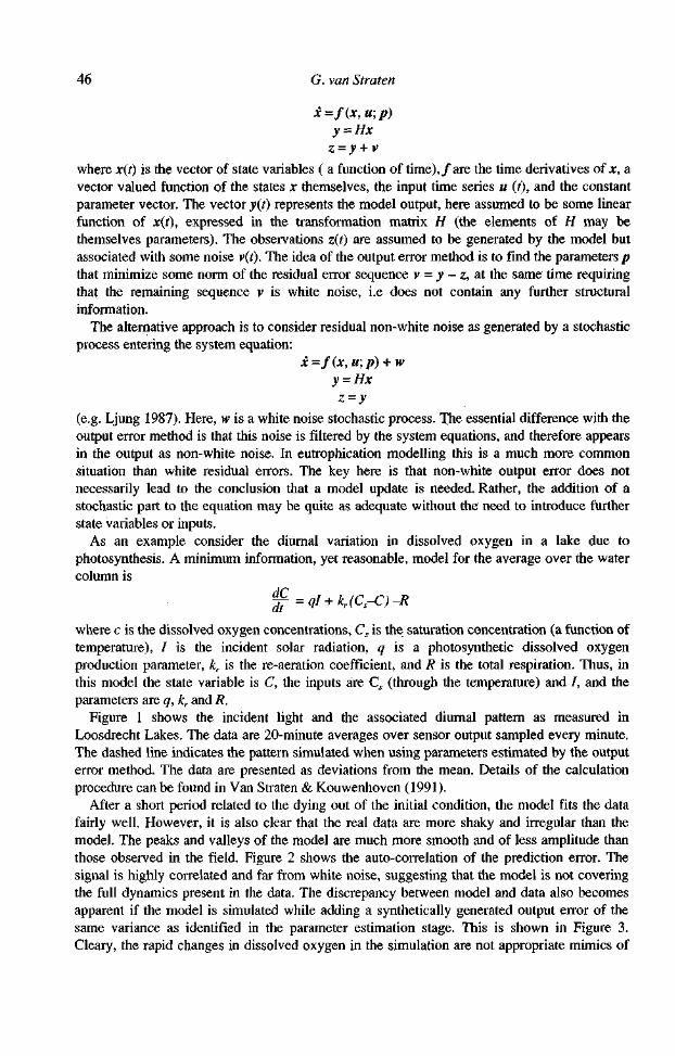
where x(t) is the vector of state variables ( a function of time), f are the time derivatives of x, a vector valued function of the states x themselves, the input time series u (t), and the constant parameter vector. The vector y(t) represents the model output, here assumed to be some linear function of x(t), expressed in the transformation matrix H (the elements of H may be themselves parameters). The observations z(t) are assumed to be generated by the model but associated with some noise v(t). The idea of the output error method is to find the parameters p that minimize some norm of the residual error sequence v = y - z, at the same time requiring that the remaining sequence v is white noise, i.e does not contain any further structural information.

The alternative approach is to consider residual non-white noise as generated by a stochastic process entering the system equation:

(e.g. Ljung 1987). Here, w is a white noise stochastic process. The essential difference with the output error method is that this noise is filtered by the system equations, and therefore appears in the output as non-white noise. In eutrophication modelling this is a much more common situation than white residual errors. The key here is that non-white output error does not necessarily lead to the conclusion that a model update is needed. Rather, the addition of a stochastic part to the equation may be quite as adequate without the need to introduce further state variables or inputs.

As an example consider the diurnal variation in dissolved oxygen in a lake due to photosynthesis. A minimum information, yet reasonable, model for the average over the water column is

where c is the dissolved oxygen concentrations, Cs is the saturation concentration (a function of temperature), I is the incident solar radiation, q is a photosynthetic dissolved oxygen production parameter, kr is the re-aeration coefficient, and R is the total respiration. Thus, in this model the state variable is C, the inputs are Cs (through the temperature) and I, and the parameters are q, kr and R.

Figure 1 shows the incident light and the associated diurnal pattern as measured in Loosdrecht Lakes. The data are 20-minute averages over sensor output sampled every minute. The dashed line indicates the pattern simulated when using parameters estimated by the output error method. The data are presented as deviations from the mean. Details of the calculation procedure can be found in Van Straten & Kouwenhoven (1991).

After a short period related to the dying out of the initial condition, the model fits the data fairly well. However, it is also clear that the real data are more shaky and irregular than the model. The peaks and valleys of the model are much more smooth and of less amplitude than those observed in the field. Figure 2 shows the auto-correlation of the prediction error. The signal is highly correlated and far from white noise, suggesting that the model is not covering the full dynamics present in the data. The discrepancy between model and data also becomes apparent if the model is simulated while adding a synthetically generated output error of the same variance as identified in the parameter estimation stage. This is shown in Figure 3. Cleary, the rapid changes in dissolved oxygen in the simulation are not appropriate mimics of


Figure 1. Solar radiation input (upper) and dissolved oxygen concentration (DO), measured (lower, solid line) and simulated with output error parameter estimates (lower, dashed line). DO (mg 1-1) is shown as deviations from the mean concentration (approximately equal to saturation in this case), plotted against time.

Figure 3. Sample noisy simulation with output error model (broken line) and deviations from the measured mean dissolved oxygen concentration (solid line; as in Fig. 1.)

Figure 2. Correlation of residual error, i.e. difference between one-step-ahead prediction and measured value.

G. van Straten 48

what happens in the field. The usual procedure is now to reject the model and to look for other explanatory factors. In

this case one might think of variations in re-aeration rate due to wind, or horizontal transport of patches of algae by wind-induced currents. A much more complicated model would be needed. As outlined above an alternative, however, would be first to look for other models for the stochastic part of the system's behaviour, for instance in terms of an equation error model:


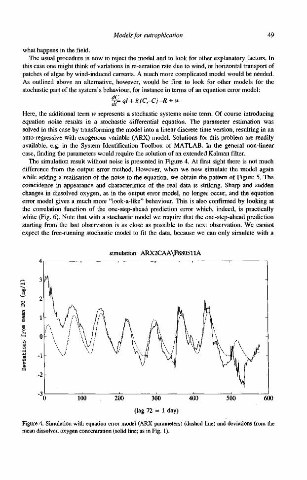
Here, the additional term w represents a stochastic systems noise term. Of course introducing equation noise results in a stochastic differential equation. The parameter estimation was solved in this case by transforming the model into a linear discrete time version, resulting in an auto-regressive with exogenous variable (ARX) model. Solutions for this problem are readily available, e.g. in the System Identification Toolbox of MATLAB. In the general non-linear case, finding the parameters would require the solution of an extended Kalman filter.

The simulation result without noise is presented in Figure 4. At first sight there is not much difference from the output error method. However, when we now simulate the model again while adding a realisation of the noise to the equation, we obtain the pattern of Figure 5. The coincidence in appearance and characteristics of the real data is striking. Sharp and sudden changes in dissolved oxygen, as in the output error model, no longer occur, and the equation error model gives a much more "look-a-like" behaviour. This is also confirmed by looking at the correlation function of the one-step-ahead prediction error which, indeed, is practically white (Fig. 6). Note that with a stochastic model we require that the one-step-ahead prediction starting from the last observation is as close as possible to the next observation. We cannot expect the free-running stochastic model to fit the data, because we can only simulate with a

Figure 4. Simulation with equation error model (ARX parameters) (dashed line) and deviations from the mean dissolved oxygen concentration (solid line; as in Fig. 1).

Figure 6. Correlation of residual error for equation error model.

Figure 5. Sample noisy simulation with equation error model, plotted as deviations from the mean dissolved oxygen concentration (as in Fig. 1).

G. van Straten 50


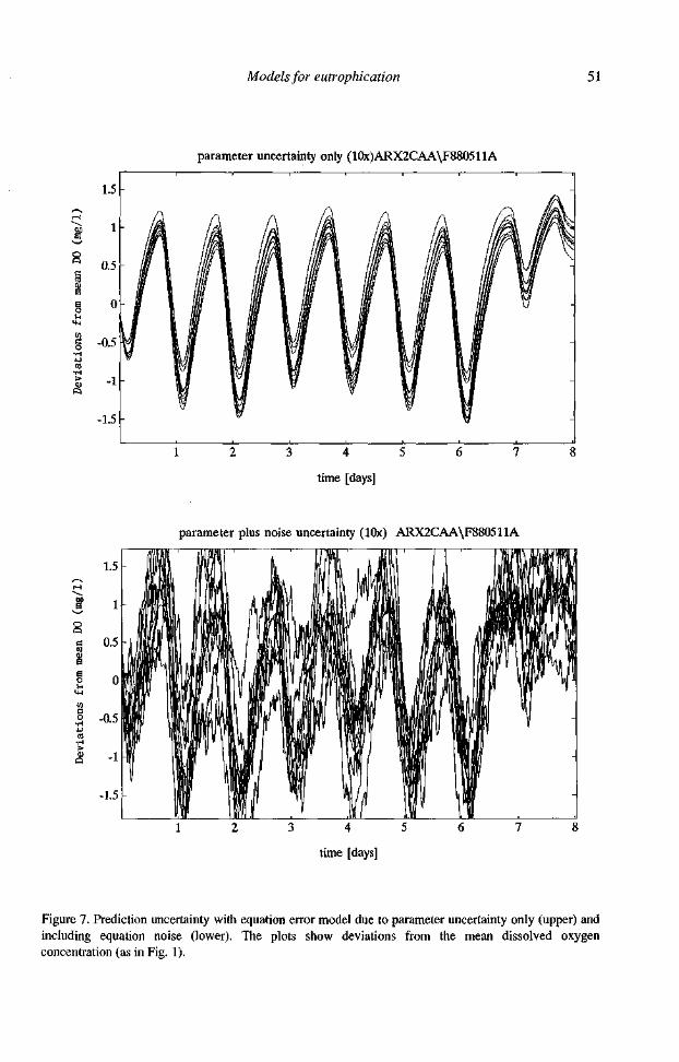
Figure 7. Prediction uncertainty with equation error model due to parameter uncertainty only (upper) and including equation noise (lower). The plots show deviations from the mean dissolved oxygen concentration (as in Fig. 1).

52 G. van Straten

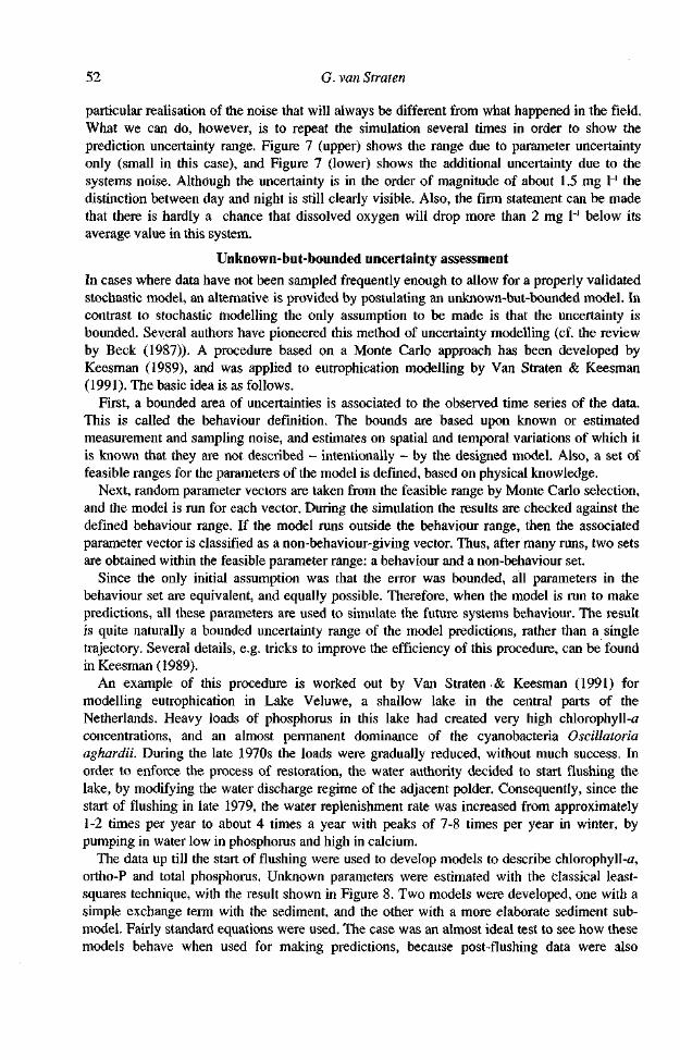
particular realisation of the noise that will always be different from what happened in the field. What we can do, however, is to repeat the simulation several times in order to show the prediction uncertainty range. Figure 7 (upper) shows the range due to parameter uncertainty only (small in this case), and Figure 7 (lower) shows the additional uncertainty due to the systems noise. Although the uncertainty is in the order of magnitude of about 1.5 mg l-1 the distinction between day and night is still clearly visible. Also, the firm statement can be made that there is hardly a chance that dissolved oxygen will drop more than 2 mg l-1 below its average value in this system.

Unknown-but-bounded uncertainty assessment

In cases where data have not been sampled frequently enough to allow for a properly validated stochastic model, an alternative is provided by postulating an unknown-but-bounded model. In contrast to stochastic modelling the only assumption to be made is that the uncertainty is bounded. Several authors have pioneered this method of uncertainty modelling (cf. the review by Beck (1987)). A procedure based on a Monte Carlo approach has been developed by Keesman (1989), and was applied to eutrophication modelling by Van Straten & Keesman (1991). The basic idea is as follows.

First, a bounded area of uncertainties is associated to the observed time series of the data. This is called the behaviour definition. The bounds are based upon known or estimated measurement and sampling noise, and estimates on spatial and temporal variations of which it is known that they are not described - intentionally - by the designed model. Also, a set of feasible ranges for the parameters of the model is defined, based on physical knowledge.

Next, random parameter vectors are taken from the feasible range by Monte Carlo selection, and the model is run for each vector. During the simulation the results are checked against the defined behaviour range. If the model runs outside the behaviour range, then the associated parameter vector is classified as a non-behaviour-giving vector. Thus, after many runs, two sets are obtained within the feasible parameter range: a behaviour and a non-behaviour set.

Since the only initial assumption was that the error was bounded, all parameters in the behaviour set are equivalent, and equally possible. Therefore, when the model is run to make predictions, all these parameters are used to simulate the future systems behaviour. The result is quite naturally a bounded uncertainty range of the model predictions, rather than a single trajectory. Several details, e.g. tricks to improve the efficiency of this procedure, can be found in Keesman (1989).

An example of this procedure is worked out by Van Straten & Keesman (1991) for modelling eutrophication in Lake Veluwe, a shallow lake in the central parts of the Netherlands. Heavy loads of phosphorus in this lake had created very high chlorophyll-a concentrations, and an almost permanent dominance of the cyanobacteria Oscillatoria aghardii. During the late 1970s the loads were gradually reduced, without much success. In order to enforce the process of restoration, the water authority decided to start flushing the lake, by modifying the water discharge regime of the adjacent polder. Consequently, since the start of flushing in late 1979, the water replenishment rate was increased from approximately 1-2 times per year to about 4 times a year with peaks of 7-8 times per year in winter, by pumping in water low in phosphorus and high in calcium.

The data up till the start of flushing were used to develop models to describe chlorophyll-a, ortho-P and total phosphorus. Unknown parameters were estimated with the classical least-squares technique, with the result shown in Figure 8. Two models were developed, one with a simple exchange term with the sediment, and the other with a more elaborate sediment sub-model. Fairly standard equations were used. The case was an almost ideal test to see how these models behave when used for making predictions, because post-flushing data were also

Figure 8. Least-squares fit to measured data (dots) for chlorophyll-a (upper) and orthophosphate-P (lower) in Lake Veluwe, using only the pre-flushing data (1978-1979) fitted to Model I (dashed lines) and Model II (solid lines). Predictions are extrapolated into 1980-1981. Measured data for the latter period are shown in Fig. 9.


G. van Straten 54

Figure 9. Unknown-but-bounded ranges for Model I (dashed lines) and Model II (solid lines). Estimations are based on measured data for pre-flushing period in 1978-1979 (see Fig. 8). Prediction uncertainty for the post-flushing period is also shown against the measured data (dots) for chlorophyll-a (upper) and orthophosphate (PO4-P; lower).


available. Comparing the predictions with actual observations show that the models did not make very accurate predictions, despite a seemingly good fit in the pre-flushing period.

To assess the uncertainties, an unknown-but-bounded approach using the same data was undertaken as well. This is shown in Figure 9. Larger uncertainty areas were obtained for Model I, because the initially set "acceptable" uncertainty band of 300 mg m-3 chlorophyll-a was not sufficient. This shows that uncertainties can be reduced by incorporating more details in the models, at the expense of more state variables and more data (for Model II, sediment dissolved oxygen consumption data were used as well).

The calibration uncertainties propagate into the prediction period, as shown in Figure 9 as well. By assessing uncertainties, it becomes apparent that the seemingly high precision of the deterministic predictions in Figure 8 are not justified. The interpretation of the bands given in Figure 9 is that algal peaks will go down, but that there is still a possibility of fairly large values even after flushing. On the other hand, the plots show that there is, in fact, also a possibility of very low values, not existing before the flushing was effected. So, despite large uncertainties, a manager might have decided that flushing was worth a try, a conclusion not at all apparent when using the best-fit parameters of Figure 8 without uncertainty assessment.

Educated speculation

The example of Lake Veluwe can also serve as an illustration of a problem of considerable interest in predicting environmental change in general (Beck 1991). After all, when implementing measures for eutrophication reduction we intentionally bring the system into another operating point. How can we be sure that we are dealing with the same system as before measures were taken? In the Lake Veluwe case, for instance, flushing introduced large amounts of calcium-rich water. It is quite conceivable that this had a definite effect upon the phosphorus exchange process with the sediment. The reduction of dissolved oxygen consumption due to lower settling of detritus material was taken care of in the model, but not the possible change of adsorptive capacity. Yet, having the model and knowing its assumptions does allow for speculation about non-modelled parameter changes brought about by control, which without a model would not have been possible.

In Figure 10, the results shown from Model I by reducing the apparent phosphorus equilibrium concentration in the sediment to 25% of its original value, as an educated guess of the effect of the larger calcium content of the flushing water. We see that even with the poor Model I this educated speculation leads to a predicted effect of flushing.

Principle problems of prediction in non-linear systems

As long as the questions remain rather crude, such as those related to phosphorus reduction measures, it is still possible to obtain reasonable answers since, after all, the mass balance just determines an upper limit to the biomass that can be sustained at any one moment. However, if we move into the much more intricate question of species composition or the inclusion of higher elements of the food web, things start to be more complicated. The equations used are highly non-linear. As a consequence, such models may exhibit strong initial sensitivity behaviour, catastrophic transitions between pseudo-equilibrium states, and even full chaotic behaviour. Moreover, the cyclic nature makes a proper calibration very difficult. The crux of this short third section of the paper is to make modellers aware of these intrinsic difficulties or even impossibilities of predicting the behaviour of cyclic, non-linear systems, and to stimulate further research in this area.

Nice examples of the effects of non-linearities in ecosystems models are given by Scheffer (1990). The practical interest lies in the options for active biological control. Some of Scheffer's results suggest that the shallow system consisting of algae, almost no zooplankton,

Figure 10. Educated speculation using Model I (see the text). A reduction by 75% of the equilibrium P-concentration due to flushing is assumed. Measured data (dots) are shown for chlorophyll-a (upper) and orthophosphate (PO4-P; lower) for both the pre-flushing and post-flushing periods.

G. van Straten 56


Figure 11. Demonstration of extreme initial condition sensitivity in a simple self-shading model for cyanobacteria in a lake. Solid line A shows algal concentration in equivalent chlorophyll-a units (left-hand scale). Solid line f1 shows the light dependency factor of the vertically and daily averaged growth rate (low in summer due to inhibition). The three plots (a - c) depict the behaviour at slightly different initial concentrations of algae (Ao).

large amounts of white fish, no predatory fish, and a lack of water plants which might serve as shelter, due to the high turbidity brought about by the algae, is the natural end station of a strongly eutrophic situation, and moreover shows a remarkable robustness against load reductions. The results can be qualitatively used to promote fish control as an additional control measure, but it is extremely difficult to quantify the effects, because the dynamics are very sensitive to parameter values, and to the assumed form of the non-linearities.

A very simple model of algal blooms, assuming a light inhibition curve, as is typical for cyanobacteria, with just one single state variable, already exhibits extreme initial condition sensitivity, as is shown in Figure 11 (Van Straten 1986). Very small changes in concentrations in winter-time have a dramatic effect upon the occurrence of algae even three years later. With more species of algae, deterministic chaotic behaviour can easily be demonstrated, and since initial conditions cannot be measured with infinite accuracy, we are facing a fundamental problem of prediction in such systems. The prediction horizon is intrinsically limited, much as in predicting the weather, and if research shows that this is truly the case, then new avenues are needed to reliably use models for ecosystems management.

58 G. van Straten

Conclusions

Model uncertainties should be and can be assessed if model predictions are to be used for management. If sufficient data are available stochastic methods are well suited. Non-white residual error can sometimes conveniently be remedied by supplementing the deterministic model with an equation error type stochastic model, rather than with an output error model. If successful, this procedure is a serious alternative to cumbersome deterministic model updates with larger data demands, more costs and longer development times, which is particularly relevant if the models have to be used for management rather than research.

When data are scarce and of poor quality, the set-theoretic unknown-but-bounded approach offers an attractive alternative to stochastic modelling in order to assess uncertainties. A proper and honest uncertainty assessment upon calibration may well reveal the true - sometimes limited - significance of model forecasts, despite the tendency of these to be on the pessimistic side.

Even when there are large uncertainties, modelling offers advantages over qualitative statements when it comes to making predictions about the systems behaviour under changed management conditions. This is because engineering judgement as well as learning from the lessons of experience can be translated into educated speculation about parameter responses to future measures.

Finally, we should be aware of fundamental problems in predicting detailed time patterns of complicated ecosystems. Due to essential non-linearities we can expect chaotic behaviour and initial condition sensitivity. More research is needed to confront and reconciliate modelling with biological observation and experience based on pattern recognition and extrapolation techniques.

References

Beck, M. B. (1987). Water quality modelling: a review of the analysis of uncertainty. Water Resources Research, 23, 1393-1442.

Beck, M. B. (1991). Forecasting environmental change. Journal of Forecasting, 10, 3-19. Keesman, K. J. (1989). A set-membership approach to the identification and prediction of ill-defined systems:

application to a water quality system. PhD dissertation, University of Twente, Enschede, The Netherlands. Ljung, L. (1987). System Identification; Theory for the User. Prentice Hall, New Jersey. Scheffer, M. (1990). Simple models as useful tools for ecologists. PhD thesis, University of Utrecht, The Netherlands. Van Straten, G. (1986). Identification, uncertainty assessment and prediction in lake eutrophication. PhD thesis,

University of Twente, Enschede, The Netherlands. Van Straten, G. & Keesman, K. J. (1991). Uncertainty propagation and speculation in projective forecasts of

environmental change: a lake-eutrophication example. Journal of Forecasting, 10, 163-190. Van Straten, G. & Kouwenhoven, J. P. M. (1991). Identification of a mechanistic model for the diurnal dissolved

oxygen pattern in lakes with discrete time series analysis. Water Science and Technology, 24, (6), 17-23.

eutrophication: research and application to water...

Documents