Evaluation of Probabilistic Queries over Imprecise Data in

Constantly-Evolving Environments ∗

Reynold Cheng§,† Dmitri V. Kalashnikov‡ Sunil Prabhakar‡§ The Hong Kong Polytechnic University, Hung Hom, Kowloon, Hong Kong

Email: csckcheng@comp.polyu.edu.hk‡ Purdue University, West Lafayette, IN 47907-1398, USA

Email: dvk@uci.edu, sunil@cs.purdue.edu

Abstract

Sensors are often employed to monitor continuously changing entities like locations of moving ob-

jects and temperature. The sensor readings are reported to a database system, and are subsequently

used to answer queries. Due to continuous changes in these values and limited resources (e.g., net-

work bandwidth and battery power), the database may not be able to keep track of the actual values

of the entities. Queries that use these old values may produce incorrect answers. However, if the

degree of uncertainty between the actual data value and the database value is limited, one can place

more confidence in the answers to the queries. More generally, query answers can be augmented with

probabilistic guarantees of the validity of the answers. In this paper, we study probabilistic query

evaluation based on uncertain data. A classification of queries is made based upon the nature of the

result set. For each class, we develop algorithms for computing probabilistic answers, and provide

efficient indexing and numeric solutions. We address the important issue of measuring the quality of

the answers to these queries, and provide algorithms for efficiently pulling data from relevant sensors

or moving objects in order to improve the quality of the executing queries. Extensive experiments∗A shorter version of this paper appeared in SIGMOD 2003 (http://www.cs.purdue.edu/homes/ckcheng/papers/sigmod03.pdf).

This manuscript contains, among others, the following new materials: (1) A new section (Section 5) on efficient evaluation

of probabilistic queries, where disk-based uncertainty indexing and numerical methods are examined; (2) New sets of

experimental results (Section 7) in a more realistic simulation model; (3) A method based on time-series analysis for

obtaining a probability density function in the uncertainty model (Appendix A); (4) Enhancement of probability query

evaluation algorithms to handle special cases of uncertainty in Appendix B; and (3) Discussions on future work in

Section 9, as well as more detailed examples.†Corresponding author.

1

are performed to examine the effectiveness of several data update policies.

Index Terms: Data Uncertainty, Constantly-Evolving Environments, Probabilistic Queries, Query

Quality, Entropy, Data Caching

1 Introduction

Sensors are often used to perform continuous monitoring over the status of an environment. The sensor

readings are then reported to the application for making decisions and answering user queries. For

example, an air-conditioning system in a building may employ temperature sensors to adjust tempera-

ture in each office. An aircraft is equipped with sensors to track the wind speed, and radars are used

to detect and report the aircraft’s location to a military system. These applications usually include a

database or server to which sensor readings are sent. Limited network bandwidth and battery power

imply that it is often not practical for the server to record the exact status of an entity it monitors at

every time instant. In particular, if the value of an entity (e.g., temperature, location) being monitored

is constantly evolving, the recorded data value may differ from the actual value. The correct value of a

sensor’s reading is known only when an update is received, and the database is only an estimate of the

actual state of the environment at most times. Specifically, there is an inherent uncertainty associated

with the constantly-changing sensor data received.

Bound for Current TemperatureRecorded Temperature

Possible Current Temperature

(c)(a) (b)

x x y x y

x0

y

y0y0

x0

y0

y1

x0

x1

Figure 1: Example of sensor data and uncertainty.

This inherent uncertainty of data affects the accuracy of answers to queries. Figure 1(a) illustrates

a query that determines the sensor (either x or y) that reports the lower temperature reading. Based

upon the data available in the database (x0 and y0), the query returns “x” as the result. In reality, the

2

temperature readings could have changed to values x1 and y1, in which case “y” is the correct answer.

Sistla et. al [1] identify this type of data as a dynamic attribute, whose value changes over time even if

it is not explicitly updated in the database. In this example, the database incorrectly assumes that the

recorded value is the actual value and produces incorrect results.

Given the uncertainty of the data, providing meaningful answers appears to be a futile exercise.

However, one can argue that in many applications, the values of objects cannot change drastically in a

short period of time; instead, the degree and/or rate of change of an object may be constrained. For

example, the temperature recorded by a sensor may not change by more than a degree in 5 minutes.

Such information can help solve the problem. Consider the above example again. Suppose we can

provide a guarantee that at the time the query is evaluated, the actual values monitored by x and y

could be no more than some deviations, dx and dy, from x0 and y0, respectively, as shown in Figure

1(b). With this information, we can state with confidence that x yields the minimum value.

In general, the uncertainty of the objects may not allow us to identify a single object that has the

minimum value. For example, in Figure 1(c), both x and y have the possibility of recording the minimum

value since the reading of x may not be lower than that of y. A similar situation exists for other types of

queries such as those that request a numerical value (e.g., “What is the lowest temperature reading?”),

where providing a single value may be infeasible due to the uncertainty in each object’s value. Instead

of providing a definite answer, the database can associate different levels of confidence with each answer

(e.g., as a probability) based upon the uncertainty of the queried objects.

The idea of probabilistic answers to queries over uncertain data in a constantly-changing database

(such as sensors and moving-object database) was briefly studied by Wolfson et. al [2]. They considered

range queries in the context of a moving object database. The objects were assumed to move in straight

lines with a known average speed. The answers to the queries consist of objects’ identities and the

probability that each object is located in the specified range. Cheng et. al [3] considered the problem of

answering probabilistic nearest neighbor queries under a moving-object database model. In this paper

we extend the notion of probabilistic queries to cover a much broader class of queries, which include

aggregate queries that compute answers over a number of objects. We also discuss the importance

of the nature of answers requested by a query (identity of object versus the value). For example,

we show that there is a significant difference between the following two queries: “Which object has

the minimum temperature?” versus “What is the minimum temperature?”. Our proposed uncertainty

model is general and it can be adapted easily to a vast class of applications dealing with constantly-

changing environments. Our techniques are also compatible with common models of uncertainty that

3

have been proposed elsewhere e.g., [2] and [4].

The probabilities in the answer allow the user to place appropriate confidence in the answer as

opposed to having an incorrect answer or no answer at all. Depending upon the application, one may

choose to report only the object with the highest probability as having the minimum value, or only

those objects whose probability exceeds a minimum probability threshold. Our proposed work will be

able to work with any of these models.

Answering aggregate queries like minimum is much more challenging than range queries in the

presence of uncertainty. The answer to a probabilistic range query consists of a set of objects along with

a non-zero probability that the object lies in the query range. Each object’s probability is determined by

the uncertainty of the object’s value and the query range. For aggregate queries, the interplay between

multiple objects is critical. The resulting probabilities are influenced by the uncertainty of other objects’

attribute values. For example, in Figure 1(c) the probability that x has the minimum value is affected

by the relative value and bounds for y. In this paper we investigate how such queries are evaluated,

with the aid of the Velocity-Constrained Index [5] and numerical techniques.

A probabilistic answer also reflects a certain level of uncertainty that results from the uncertainty of

the queried object values. If the uncertainty of all (or some) of the objects was reduced (or eliminated

completely), the uncertainty of the result improves. For example, without any knowledge about the

value of an object, one could arguably state that it falls within a query range with 50% probability.

On the other hand, if the value is known perfectly, one can state with 100% confidence that the object

either falls within or outside the query range. Thus the quality of the result is measured by degree of

ambiguity in the answer. We therefore need metrics to evaluate the quality of a probabilistic answer.

We propose metrics for evaluating the quality of the probabilistic answers. As we shall see, different

metrics are suitable for different classes of queries.

The quality of a query result may not be acceptable for certain applications – a more definite result

may be desirable. Since the poor quality is directly related to the uncertainty in the object values,

one possibility for improving the results is to delay the query until the quality improves. However

this is an unreasonable solution due to the increased query response time. Instead, the database could

request updates from all objects (e.g., sensors) – this solution incurs a heavy load on the resources. In

this paper, we propose to request updates only from objects that are being queried, and furthermore

those that are likely to improve the quality of the query result. We present some heuristics and an

experimental evaluation. These policies attempt to optimize the use of the constrained resource (e.g.,

4

network bandwidth to the server) to improve average query quality. We also examine the relationship

between network bandwidth usage and probabilistic queries, as well as the scenario when queries with

contradicting properties are concurrently executed.

It should be noted that the imprecision in the query answers is inherent in this problem (due to

uncertainty in the actual values of the dynamic attribute), in contrast to the problem of providing

approximate answers for improved performance wherein accuracy is traded for efficiency. To sum up,

the contributions of this paper are:

• A general data model to capture uncertainty of constantly-evolving data;

• A broad classification of probabilistic queries over uncertain data;

• Efficient evaluation techniques for probabilistic queries;

• Metrics for quantifying the quality of answers to probabilistic queries;

• Policies for improving quality of probabilistic answers under resource constraints; and

• Experimental results on performance of probabilistic queries.

The rest of this paper is organized as follows. In Section 2 we describe a general model of uncertainty,

and the concept of probabilistic queries. Sections 3 and 4 discuss the algorithms for evaluating different

kinds of probabilistic queries. In Section 5, indexing and numeric methods for handling practical

issues of query evaluation are discussed. Section 6 discusses quality metrics that are appropriate to

these queries, and proposes update policies that improve the query answer quality. We present an

experimental evaluation of the effectiveness of these update policies in Section 7. Section 8 discusses

related work and Section 9 concludes the paper.

2 Probabilistic Queries

In this section, we describe the model of uncertainty considered in this paper. This is a generic model,

as it can accommodate a large number of application paradigms. Based on this model, we introduce a

number of probabilistic queries.

5

2.1 Uncertainty Model

One popular model for uncertainty for a dynamic attribute is that at any point in time, the actual value

is within a certain bound, d of its last reported value. If the actual value changes further than d, then

the sensor reports its new value to the database and possibly changes d. For example, [2] describes

a moving-object model where the location of an object is a dynamic attribute, and an object reports

its location to the server if its deviation from the last reported location exceeds a threshold. Another

model assumes that the attribute value changes with known speed, but the speed may change each time

the value is reported. Other models include those that have no uncertainty. For example, in [4], the

exact speed and direction of movement of each object are known. This model requires updates at the

server whenever an object’s speed or direction changes.

For the purpose of our discussion, the exact model of uncertainty is unimportant. All that is required

is that at the time of query execution the range of possible values of the attribute of interest are known.

We are interested in queries over some dynamic attribute, a, of a set of database objects, T . Also,

we assume that a is a real-valued attribute, but our models and algorithms can be extended to other

domains e.g., integer, and higher dimensions e.g, 2-D uncertainty and queries in [3]. We denote the

ith object of T by Ti and the value of attribute a of Ti by Ti.a (where i = 1, . . . , |T |). Throughout

this paper, we treat Ti.a’s as independent continuous random variables. The uncertainty of Ti.a can be

characterized by the following two definitions (we use pdf to abbreviate the term “probability density

function”):

Definition 1: An uncertainty interval of Ti.a at time instant t, denoted by Ui(t), is an interval

[li(t), ui(t)] such that li(t) and ui(t) are real-valued functions of t, and that the conditions ui(t) ≥ li(t)

and Ti.a ∈ [li(t), ui(t)] always hold.

Definition 2: An uncertainty pdf of Ti.a at time t, denoted by fi(x, t), is a pdf of a random variable

Ti.a, such that fi(x, t)=0 if x /∈ Ui(t).

Since fi(x, t) is a pdf, it has the property that∫ ui(t)li(t)

fi(x, t)dx = 1. The above definition specifies the

uncertainty of Ti.a at time instant t in terms of a closed interval and the probability distribution of Ti.a

in that interval. Notice that this definition specifies neither how the uncertainty interval evolves over

time, nor what the nature of the pdf fi(x, t) is inside the uncertainty interval. The only requirement

for fi(x, t) is that its value is 0 outside the uncertainty interval. Usually, the scope of uncertainty is

determined by the last recorded value, the time elapsed since its last update, and some application-

6

specific assumptions. For example, one may decide that UA(t) contains all the values within a distance

of (t−tupdate)×v from its last reported value, where tupdate is the time that the last update was obtained,

and v is the maximum rate of change of the value.

A trivial pdf is the uniform distribution i.e., Ti.a is uniformly distributed inside Ui(t). In other

words, fi(x, t) equals to 1/[ui(t)− li(t)] for Ti.a ∈ Ui(t), assuming that ui(t) > li(t). It should be noted

that the uniform distribution represents the worst-case uncertainty, or “the most uncertain” scenario

over a given uncertainty interval. Another example of pdf is the Gaussian distribution. In general,

the exact pdf to be used is application-dependent. If the pdf is not known to the application, or a

more accurate pdf is required, we refer readers to Appendix A for a simple method of pdf estimation.

Finally, for a general pdf that cannot be expressed in arithmetic expressions, it be modeled in the form

of histograms.

2.2 Classification of Probabilistic Queries

We now present a classification of probabilistic queries and examples of common representative queries

for each class. We identify two important dimensions for classifying database queries. First, queries

can be classified according to the nature of the answers. An entity-based query returns a set of objects

that satisfy the condition of the query. A value-based query returns a single value, examples of which

include querying the value of a particular sensor, and computing the average value of a subset of sensor

readings. The second criterion for classifying queries is based on whether “aggregation” is involved.

We use the term aggregation loosely to refer to queries where interplay between objects determines

the result. In the following definitions, the first letter is either E (for entity-based queries) or V (for

value-based queries).

1. Value-based Non-Aggregate Class

This is the simplest type of query in our discussions. It returns an attribute value of an object as

the only answer, and involves no aggregate operators. One example of a probabilistic query for this

class is the VSingleQ:

Definition 3: Probabilistic Single Value Query (VSingleQ) Given an object Tk, a VSingleQ

returns l, u, {p(x) | x ∈ [l, u]} where l, u ∈ % with l ≤ u, and p(x) is the pdf of Tk.a such that p(x) = 0

when x < l or x > u.

An example of VSingleQ is “What is the wind speed recorded by sensor s22?” Observe how this

7

definition expresses the answer in terms of a bounded probabilistic value, instead of a single value. Also

notice that∫ ul p(x)dx = 1.

2. Entity-based Non-Aggregate Class

This type of query returns a set of objects, each of which satisfies the condition(s) of the query,

independent of other objects. A typical example is a query that returns a set of objects satisfying a

user-specified interval:

Definition 4: Probabilistic Range Query (ERQ) Given a closed interval [l, u], where l, u ∈ % and

l ≤ u, an ERQ returns a set of tuples (Ti, pi), where pi is the non-zero probability that Ti.a ∈ [l, u].

An ERQ can be used in sensor networks and location monitoring. An example ERQ is ask which

sensor(s) return temperature values that are within a user-specified interval.

3. Entity-based Aggregate Class

The third class of query returns a set of objects which satisfy an aggregate condition. We present

the definitions of three typical queries for this class.

Definition 5: Probabilistic Minimum (Maximum) Query (EMinQ (EMaxQ)) An EMinQ

(EMaxQ) returns a set R of tuples (Ti, pi), where pi is the non-zero probability that Ti.a is the minimum

(maximum) value of a among all objects in T .

Definition 6: Probabilistic Nearest Neighbor Query (ENNQ) Given a value q ∈ %, an ENNQ

returns a set R of tuples (Ti, pi), where pi is the non-zero probability that |Ti.a − q| is the minimum

among all objects in T .

These queries have wide application in aggregating information in data streams sensor networks.

For example, one may want to acquire the identity of the sensor that yields the maximum temperature

value over a region being monitored by sensors [6]. Nearest neighbor queries have also been widely used

in location databases [7]. Notice that for all these queries the condition∑

Ti∈R pi = 1 holds.

4. Value-based Aggregate Class

The final class involves aggregate operators that return a single value. Examples include:

8

Query Class Entity-based Value-based

Aggregate ENNQ, EMinQ, EMaxQ VAvgQ, VSumQ, VMinQ, VMaxQ

Non-Aggregate ERQ VSingleQ

Answer (Probabilistic) {(Ti, pi) | 1 ≤ i ≤ |T | ∧ pi > 0} l, u, {p(x) | x ∈ [l, u]}

Answer (Non-probabilistic) {Ti | 1 ≤ i ≤ |T |} x | x ∈ $

Table 1: Classification of Probabilistic Queries.

Definition 7: Probabilistic Average (Sum) Query (VAvgQ (VSumQ)) A VAvgQ (VSumQ)

returns l, u, {p(x) | x ∈ [l, u]}, where l, u ∈ % with l ≤ u, X is a random variable for the average (sum)

of the values of a for all objects in T , and p(x) is a pdf of X satisfying p(x) = 0 if x < l or x > u.

Definition 8: Probabilistic Minimum (Maximum) Value Query (VMinQ (VMaxQ)) A VMinQ

(VMaxQ) returns l, u, {p(x) | x ∈ [l, u]} where l, u ∈ % with l ≤ u, X is a random variable for minimum

(maximum) value of a among all objects in T , and p(x) is a pdf of X satisfying p(x) = 0 if x < u or

x > l.

One typical example of these queries is to inquire about the minimum pressure value among all the

sensors in a monitoring sensor network [6]. All these aggregate queries return answers in the form of a

probabilistic distribution p(x) in a closed interval [l, u], such that∫ ul p(x)dx = 1.

Table 1 summarizes the basic properties of the probabilistic queries discussed above. For illustrating

the difference between probabilistic and non-probabilistic queries, the last row of the table lists the forms

of answers expected if probability information is not augmented to the result of the queries e.g., the

non-probabilistic version of EMaxQ is a query that returns object(s) with maximum values based only

on the recorded values of Ti.a.1 It can be seen that the probabilistic queries provide more information

on the answers than their non-probabilistic counterparts.

Example. We illustrate the properties of the probabilistic queries with a simple example. In Figure 2,

readings of four sensors s1, s2, s3 and s4, each with a different uncertainty interval, are being queried at

time t0. Suppose we have a set T of four database objects to record the information of these sensors,

and each object has an attribute a to store the sensor reading. Moreover, assume that for each reading,

its actual value has the same chance of being located at every point in its uncertainty interval, and the

actual value has no chance of lying outside the interval i.e., fsi(x, t0) (where i = 1, . . . , 4) is a bounded

uniform distribution function. Also denote the uncertainty interval of si at time t0 be [lsi , usi ]. A1The non-probabilistic version of EMaxQ may return more than one object if their values are both equal to the maximum

value.

9

Recorded Value

Bound for

Current Value

q

l

us2

s1

s4

s3

Figure 2: Illustrating the probabilistic queries.

VSingleQ applied on s4 at time t0 will give us the result: ls4 , us4 , 1/(us4 − ls4). Now suppose an ERQ

(represented by the interval [l, u]) is invoked at time t0 to find out how likely each reading is inside

[l, u] = [1, 15], and the uncertainty intervals derived from the readings of s1, s2, s3 and s4 at time t0 are

[2, 12], [8, 18], [11, 21] and [25, 30] respectively. Since the reading of s1 is always inside [l, u], , it has a

probability of 1 for satisfying the ERQ. The reading of s4 is always outside [l, u], thus it has a probability

of 0 of being located inside [l, u]. Since Us2(t0) and Us3(t0) partially overlap [l, u], s2 and s3 have some

chance of satisfying the query. In this example, the result of the ERQ is: {(s1, 1), (s2, 0.7), (s3, 0.4)}.

In the same figure, an EMinQ is issued at time t0. We observe that s1 has a high probability of having

the minimum value, because a large portion of the Us1(t0) has a smaller value than others. The reading

of s1 has a high chance of being located in this portion because fs1(x, t) is a uniform distribution. The

reading of s4 does not have any chance of yielding the minimum value, since none of the values inside

Us4(t0) is smaller than others. The result of the EMinQ for this example is: {(s1, 0.7), (s2, 0.2), (s3, 0.1)}.

On the other hand, an EMaxQ will return {(s4, 1)} as the only result, since every value in Us4(t0) is

higher than any readings from any other sensors, and we are assured that s4 yields the maximum value.

An ENNQ with a query value q = 13 is also shown, where the results are: {(s1, 0.2), (s2, 0.5), (s3, 0.3)}.

When a value-based aggregate query is applied to the scenario in Figure 2, a bounded pdf p(x) is

returned. If a VSumQ is issued, the result is a distribution in [ls1 + ls2 + ls3 + ls4 , us1 + us2 + us3 + us4 ];

each x in this interval is the sum of the readings from the four sensors. The result of a VAvgQ is a pdf

in [(ls1 + ls2 + ls3 + ls4)/4, (us1 + us2 + us3 + us4)/4]. The results of VMinQ and VMaxQ are probability

distributions in [ls1 , us1 ] and [ls4 , us4 ] respectively, since only the values in these ranges have a non-zero

probability value of satisfying the queries.

10

3 Evaluating Entity-based Queries

In this section we examine how the probabilistic entity-based queries introduced in the last section

can be answered. We start with the discussion of an ERQ, followed by a more complex algorithm for

answering an ENNQ. We also show how the algorithm for answering an ENNQ can be easily changed

for EMinQ and EMaxQ.

3.1 Evaluation of ERQ

Recall that ERQ returns a set of tuples (Ti, pi) where pi is the non-zero probability that Ti.a is within

a given interval [l, u]. To evaluate an ERQ at time instant t, each object’s pi is computed as follows:

first, the amount of overlap OI between Ui(t) and [l, u] is found (i.e., OI = Ui(t) ∩ [l, u]). 2 If OI has

zero width, we are assured that Ti.a does not lie in [l, u], and thus pi = 0 and Ti will not be included in

the result. Otherwise, we calculate the probability that Ti.a is inside [l, u] by integrating fi(x, t) over

OI (i.e., pi =∫OI fi(x, t)dx), and return the result (Ti, pi) if pi (= 0.

3.2 Evaluation of ENNQ

U4 U4

n4n3

U3

U1

n1

U4

!10T3.aT4.a !15

T5.a

f

f

f

f

f

T1.a 20

(a) (b)

q

(c) (d)

U1

n1

n3

U3

n4

q

q

n4n3

T5.a

q 10

60

T4.aT3.a

U3

n5

n1

T1.a

U1

T2.a

n2

U2

U5

T2.a 25

n2

U2

n2

U2

Figure 3: Illustrating the ENNQ algorithm.

2Appendix B discusses the special case for l = u.

11

Processing an ENNQ involves evaluating the probability of the attribute a of each object Ti being

the closest to (nearest-neighbor of) a value q. Unlike the case of ERQ, we can no longer determine

the probability for an object independent of the other objects. Recall that an ENNQ returns a set of

tuples (Ti, pi) where pi denotes the non-zero probability that Ti has the minimum value of |Ti.a − q|.

Let S be the set of objects to be considered by the ENNQ, and R be the set of tuples returned by the

query. The algorithm presented here consists of three phases: pruning, bounding and evaluation. The

first two phases filter out objects in T whose values of a have no chance of being the closest to q. The

final phase, evaluation, is the core of our solution: for every Ti that remains, the probability that Ti is

the nearest neighbor of q is computed.

1. for i ← 1 to |S| do

(a) if (q ∈ Ui(t)) then Ni ← q

(b) else

i. if (|q − li(t)| < |q − ui(t)|) then Ni ← li(t)

ii. else Ni ← ui(t)

(c) if (|q − li(t)| < |q − ui(t)|) then Fi ← ui(t)

(d) else Fi ← li(t)

2. Let f = mini=1,...,|S||Fi − q| and m = |S|3. for i ← 1 to m do

if (|Ni − q| > f) then S ← S − Ti

4. return S

Figure 4: Algorithm for the Pruning Phase.

1. Pruning Phase. Consider two uncertainty intervals U1(t) and U2(t). If the smallest difference

between U1(t) and q is larger than the largest difference between U2(t) and q, we can immediately

conclude that T1 is not part of the answer to the ENNQ: even if the actual value of T2.a is as far as

possible from q, T1.a still has no chance to be closer to q than T2.a. Based on this observation, we can

eliminate objects from T by the algorithm shown in Figure 4. In this algorithm, Ni and Fi record the

closest and farthest possible values of Ti.a to q, respectively. Steps 1(a) to 1(d) assign proper values to

Ni and Fi. If q is inside interval Ui(t), then Ni is taken as point q itself. Otherwise, Ni is either li(t)

or ui(t), depending on which value is closer to q. Fi is assigned in a similar manner. After this phase,

S contains the minimal set of objects that must be considered by the query; any of them can have a

value of Ti.a closest to q. Figure 3(a) shows the last recorded values of Ti.a in S at time t0, and the

12

uncertainty intervals are shown in Figure 3(b). We also see how T5 is removed from consideration since

there is at least one uncertainty interval completely closer than it. Figure 3(c) shows the result of this

phase.

2. Bounding Phase. For each object in S, we only need to look at its portion of uncertainty interval

located no farther than f from q. We do this conceptually by drawing a bounding interval B of length

2f , centered at q. Any portion of the uncertainty interval outside B can be ignored. Figure 3(c) shows

a bounding interval with length 2f , and Figure 3(d) illustrates the result of this phase.

3. Evaluation Phase. Based on S and the bounding interval B, our aim is to calculate, for each

object in S, the probability that it is the nearest neighbor of q. In the pruning phase, we have already

found Ni, the point in Ui(t) nearest to q. Let us call |Ni − q| by the near distance of Ti, or ni. Denote

the interval with length 2r, centered at q by Iq(r). Also, let Pi(r) be the probability that Ti is located

inside Iq(r), and pri(r) be the pdf of Ri, where Ri = |Ti.a − q|. Figure 5 presents the algorithm.

Note that if Ti.a has no uncertainty i.e., Ui(t) is exactly equal to Ti.a, the evaluation phase algorithm

needs to be modified. This issue will be discussed in Appendix B. For the rest of the discussions, we

will assume non-zero uncertainty.

1. R ← ∅2. Sort the elements in S in ascending order of ni, and

rename the sorted elements in S as T1, T2, . . . , T|S|

3. n|S|+1 ← f

4. for i ← 1 to |S| do

(a) pi ← 0

(b) for j ← i to |S| do

i. p ←∫ nj+1

njpri(r) ·

∏jk=1∧k "=i(1 − Pk(r)) dr

ii. pi ← pi + p

(c) R ← R ∪ (Ti, pi)

5. return R

Figure 5: Algorithm for the Evaluation Phase.

Evaluation of Pi(r) and pri(r). To understand how the evaluation phase works, it is crucial to

know how to obtain Pi(r). As introduced before, Pi(r) is the probability that Ti.a is located inside

13

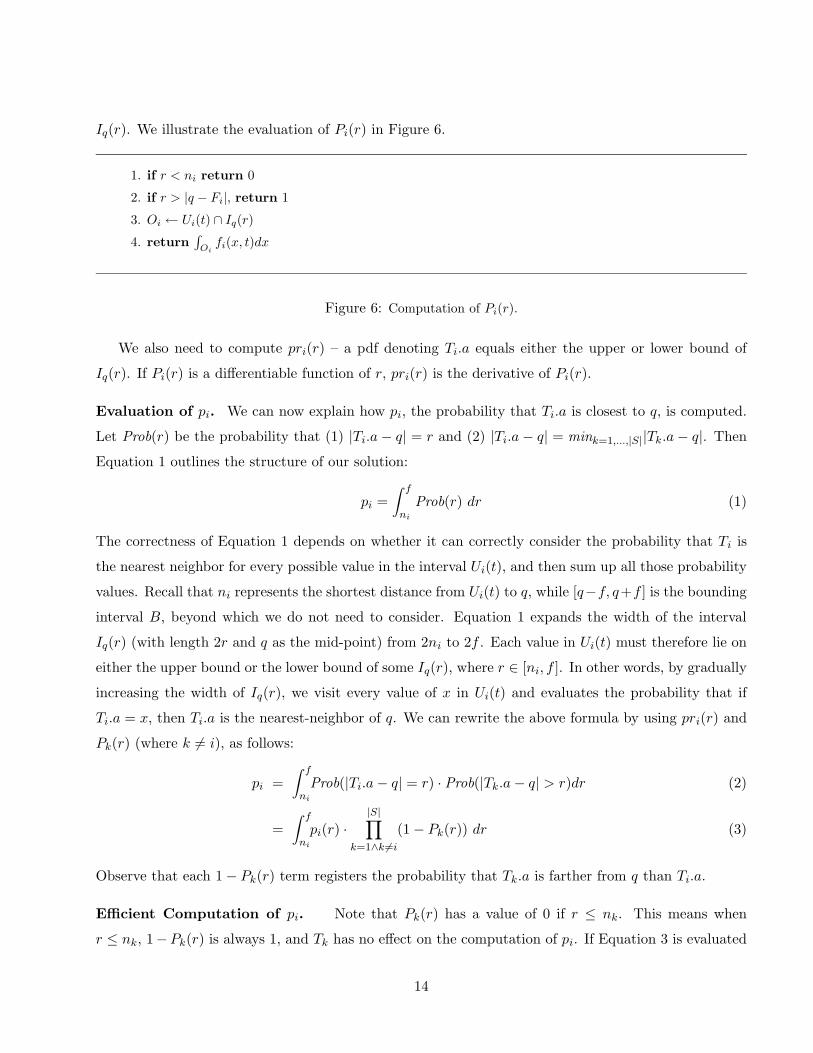
Iq(r). We illustrate the evaluation of Pi(r) in Figure 6.

1. if r < ni return 0

2. if r > |q − Fi|, return 1

3. Oi ← Ui(t) ∩ Iq(r)

4. return∫

Oifi(x, t)dx

Figure 6: Computation of Pi(r).

We also need to compute pri(r) – a pdf denoting Ti.a equals either the upper or lower bound of

Iq(r). If Pi(r) is a differentiable function of r, pri(r) is the derivative of Pi(r).

Evaluation of pi. We can now explain how pi, the probability that Ti.a is closest to q, is computed.

Let Prob(r) be the probability that (1) |Ti.a − q| = r and (2) |Ti.a − q| = mink=1,...,|S||Tk.a − q|. Then

Equation 1 outlines the structure of our solution:

pi =∫ f

ni

Prob(r) dr (1)

The correctness of Equation 1 depends on whether it can correctly consider the probability that Ti is

the nearest neighbor for every possible value in the interval Ui(t), and then sum up all those probability

values. Recall that ni represents the shortest distance from Ui(t) to q, while [q−f, q+f ] is the bounding

interval B, beyond which we do not need to consider. Equation 1 expands the width of the interval

Iq(r) (with length 2r and q as the mid-point) from 2ni to 2f . Each value in Ui(t) must therefore lie on

either the upper bound or the lower bound of some Iq(r), where r ∈ [ni, f ]. In other words, by gradually

increasing the width of Iq(r), we visit every value of x in Ui(t) and evaluates the probability that if

Ti.a = x, then Ti.a is the nearest-neighbor of q. We can rewrite the above formula by using pri(r) and

Pk(r) (where k (= i), as follows:

pi =∫ f

ni

Prob(|Ti.a − q| = r) · Prob(|Tk.a − q| > r)dr (2)

=∫ f

ni

pi(r) ·|S|∏

k=1∧k #=i

(1 − Pk(r)) dr (3)

Observe that each 1 − Pk(r) term registers the probability that Tk.a is farther from q than Ti.a.

Efficient Computation of pi. Note that Pk(r) has a value of 0 if r ≤ nk. This means when

r ≤ nk, 1−Pk(r) is always 1, and Tk has no effect on the computation of pi. If Equation 3 is evaluated

14

numerically, considering all |S|− 1 objects in the∏

term at every integration step can be unnecessarily

expensive.3 Here we present a technique to reduce the number of objects to be evaluated.

The method first sorts the objects according to their near distance from q. Next, the integration

interval [ni, f ] is broken down into a number of intervals, with end points defined by the near distance

of the objects. The probability of an object having a value of a closest to q is then evaluated for each

interval in a way similar to Equation 3, except that we only consider Tk.a with non-zero Pk(r). Then

pi is equal to the sum of the probability values for all these intervals. The final formula for pi becomes:

pi =|S|∑

j=i

∫ nj+1

nj

pri(r) ·j∏

k=1∧k #=i

(1 − Pk(r)) dr

(4)

Here we let n|S|+1 be f . Instead of considering |S| − 1 objects in the∏

term, Equation 4 only

handles j − 1 objects in interval [nj , nj + 1]. This optimization is shown in Figure 5.

Example. Let us use our previous example to illustrate how the evaluation phase works. After 4

objects T1, . . . , T4 were captured (Figure 3(d)), Figure 7 shows the result after these objects have been

sorted in ascending order of their near distance, with the r-axis being the absolute difference of Ti.a

from q, and n5 equals f . The probability pi (that Ti is the nearest neighbor of q) is equal to the integral

of the probability that Ti is the nearest neighbor over the interval [ni, n5].

U4

U3

U2

U1

n2n1 n n3 40 5n = f

r

Figure 7: Illustrating the evaluation phase.

Let us see how we evaluate uncertainty intervals when computing p2. Equation 4 tells us that p2

is evaluated by integrating over [n2, n5]. Since objects are sorted according to ni, we do not need to

consider all 5 of them throughout [n2, n5]. Instead, we split [n2, n5] into 3 sub-intervals, namely [n2, n3],

[n3, n4] and [n4, n5]. Then we only need to consider uncertainty intervals U1, U2 in the range [n2, n3],

U1, U2, U3 in the range [n3, n4], and U1, U2, U3, U4 in the range [n4, n5].3The issues of using numerical integration to compute Equation 3 are discussed again in Section 5.2.

15

For T2 to be the nearest neighbor of q in [n3, n4], we require that (1) T2.a is inside [n3, n4], and,

(2) T1.a and T3.a are farther than T2.a from q. The first condition is captured by pri(r)dr, and the

second one is represented by∏j

k=1∧k #=i(1 − Pk(r)) in Equation 4. Therefore, the probability that T2 is

the nearest neighbor in [n3, n4] is∫ n4n3

pr2(r) · (1 − P1(r)) · (1 − P3(r))dr. The final value of p2 is equal

to the sum of the probability values over the 3 intervals:

p2 =∫ n3n2

pr2(r)(·1−P1(r)) dr +∫ n4n3

pr2(r) ·∏

k=1,3(1−Pk(r)) dr +∫ n5n4

pr2(r) ·∏

k=1,3,4(1−Pk(r)) dr

3.3 Evaluation of EMinQ and EMaxQ

Answering an EMinQ is equivalent to answering an ENNQ with q equal to the minimum lower bound

of all Ui(t) in T . We can therefore modify the ENNQ algorithm to solve an EMinQ by evaluating the

minimum value of li(t) among all uncertainty intervals. Then we set q to that value. We then obtain

the results to the EMinQ by using the same ENNQ algorithm. Solving an EMaxQ is symmetric to

solving an EMinQ in which we set q to the maximum of ui(t).

4 Evaluating Value-based Queries

4.1 Evaluation of VSingleQ

Evaluating a VSingleQ is simple, since by the definition of VSingleQ, only one object, Tk, needs to

be considered. Suppose VSingleQ is executed at time t. Then the answer returned is the uncertainty

information of Tk.a at time t, i.e., lk(t), uk(t) and {fk(x, t)|x ∈ [lk(t), uk(t)]}.

4.2 Evaluation of VSumQ and VAvgQ

Let us first consider the case where we want to find the sum of two random variables with uncertainty

intervals [l1(t), u1(t)] and [l2(t), u2(t)] for objects T1 and T2. Notice that the values in the answer that

have non-zero probability values lie in the range [l1(t)+l2(t), u1(t)+u2(t)]. For any x inside this interval,

p(x) (the pdf of random variable X = T1.a + T2.a) is:

∫ min{u1(t),x−l2(t)}

max{l1(t),x−u2(t)}f1(y, t)f2(x − y, t)dy (5)

16

Suppose y ∈ [l1(t), u1(t)] where f1(y) is non-zero. If x is the sum of T1.a and T2.a, we require that

l2(t) < x − y < u2(t) so that f2(x − y) is non-zero. These two conditions are used to derive the above

integration interval where both f1 and f2 are non-zero.

We can generalize this result for summing the uncertainty intervals of |T | objects by picking two

intervals, summing them up using the above formula, and using the resulting interval to add to another

interval. The process is repeated until we finish adding all the intervals. The resulting interval should

have the following form:

[|T |∑

i=1

li(t),|T |∑

i=1

ui(t)]

VAvgQ is essentially the same as VSumQ except for a division by the number of objects over which

the aggregation is applied.

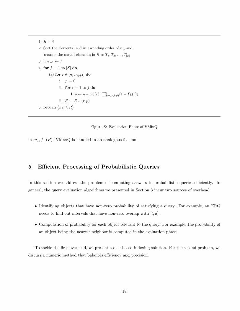
4.3 Evaluation of VMinQ and VMaxQ

To answer a VMinQ, we need to find a lower bound l, an upper bound u, and a pdf p(x) where p(x)

is the pdf of the minimum value of a. Recall from Section 3.3 that in order to answer an EMinQ, we

set q to be the minimum of the lower bound of the uncertainty intervals, and then obtain a bounding

interval B in the bounding phase, within which we explore the uncertainty intervals to find the item

with the minimum value. Interval B is exactly the interval [l, u], since B determines the region where

the possible minimum values are. In order to answer a VMinQ, we can use the first three phases of

EMinQ (projection, pruning, bounding) to find B as the interval [l, u]. The evaluation phase is replaced

by the algorithm shown in Figure 8.

Again, Steps 2 and 3 sort the objects in ascending order of ni. After these steps, B = [n1, f ]

represents the range of possible values. Step 4 evaluates p(r) for some value r sampled in [n1, f ] (the

sampling technique is discussed in Section 5.2). Since we have sorted the uncertainty intervals in

ascending order of ni, we need not consider all |T | objects throughout [n1, f ]. Specifically, for any value

r in the interval [nj , nj+1], we only need to consider objects T1, . . . , Tj in evaluating p(r). Hence for

r ∈ [nj , nj+1], p(r) is given by the following formula:

p(r) =j∑

i=1

(pri(r) ·j∏

k=1∧k #=i

(1 − Pk(r))) (6)

The pair (r, p) represents r, p(r). It is inserted into the set R in Step 4(a)iii. Finally, Step 5 returns the

lower bound (n1), upper bound (f) of the minimum value, and the distribution of the minimum values

17

1. R ← ∅2. Sort the elements in S in ascending order of ni, and

rename the sorted elements in S as T1, T2, . . . , T|S|

3. n|S|+1 ← f

4. for j ← 1 to |S| do

(a) for r ∈ [nj , nj+1] do

i. p ← 0

ii. for i ← 1 to j do

I. p ← p + pri(r) ·∏j

k=1∧k "=i(1 − Pk(r))

iii. R ← R ∪ (r, p)

5. return {n1, f, R}

Figure 8: Evaluation Phase of VMinQ.

in [n1, f ] (R). VMaxQ is handled in an analogous fashion.

5 Efficient Processing of Probabilistic Queries

In this section we address the problem of computing answers to probabilistic queries efficiently. In

general, the query evaluation algorithms we presented in Section 3 incur two sources of overhead:

• Identifying objects that have non-zero probability of satisfying a query. For example, an ERQ

needs to find out intervals that have non-zero overlap with [l, u].

• Computation of probability for each object relevant to the query. For example, the probability of

an object being the nearest neighbor is computed in the evaluation phase.

To tackle the first overhead, we present a disk-based indexing solution. For the second problem, we

discuss a numeric method that balances efficiency and precision.

18

!"#$%&&&

!"#$%&&&

!"#$%&&&

!"#$%&&&

!"#$%&&&'"()* +, -./, -./+,

'"()0 +0 -./, -./+0

+1 -./, -./+1

+2 -./, -./+2&&&

+3 -./, -./+3&&&'"()1

'"()2

'"()3

4,41 40 42 4345 46

7($(

89:!

4,

40

41

42

45

43

46

;(<=>

4(?:!

Figure 9: Structure of VCI.

5.1 Indexing Uncertainty Intervals

The execution time of a query is significantly affected by the number of objects that need to be con-

sidered. With a large database, it is impractical to evaluate each object for answering the query. In

particular, in a large database, it is impractical to retrieve the uncertainty interval for each object and

check whether the object has non-zero probability of satisfying the ERQ. Similarly, we cannot afford

checking every interval to decide the final output in the pruning phase of the ENNQ. It is therefore

important to reduce the number of objects for examination. As with traditional queries, indexes can

be used for this purpose.

Notice that in order to retrieve the required object for a VSingleQ, a disk-based hash table technique

for the IDs of objects e.g., extendible hashing is sufficient for the purpose. For VAvgQ and VSumQ, no

indexes are required because all objects in T have to be examined. Thus we do not discuss further the

indexing issues of these queries. For other queries, we will discuss a special-purpose data structure that

can facilitate their execution.

The key challenge for any indexing solution for uncertainty intervals is the efficient updating of the

index as uncertainty intervals grow (according to li(t) and ui(t)), shrink (due to an update) and then

grow again (with possibly different li(t) and ui(t)). We can view this as the problem of indexing moving

objects in one-dimensional space, where the value of the interested sensor is modeled as the location of

an object moving along a straight line. Also, the index should be simple and general enough to handle

various queries we propose. For these reasons, we have chosen the Velocity-Constrained Index (VCI)

19

originally proposed for indexing moving objects. We only briefly describe its structure and how we use

it for our queries. Interested readers are referred to [5] for further details.

In the VCI, the only restriction imposed on the data values is that the rates of growth of uncertainty

interval bounds (i.e., li(t) and ui(t)) do not exceed a certain threshold. This rate threshold could

potentially be adjusted if the sensor wants to change its value faster than its current maximum rate.

The maximum growing rates of uncertainty intervals of all objects are used in the construction of the

index. The VCI is an one-dimensional R-tree-like index structure. It differs from the R-tree in that each

node has an additional field: Rmax – the maximum possible rate of change over all the objects that fall

under that node. The index is initiated by the sensor values at a given point in time, t0. Construction

is similar to the R-tree except that the field Rmax at every node is always adjusted to ensure that it is

equal to the largest rate of change of Ti.a for all Ti’s in the sub-tree. Upon the split of a node, the Rmax

entry is simply copied to the new node. At the leaf level the maximum growing rate of each indexed

uncertainty interval is stored (not just the maximum growing rate of the leaf node). Figure 9 illustrates

an example of VCI.

As a new sensor update is received, its value is noted in the database (which can be done by using

a secondary index like a hash table). However, no change is made to the VCI. When the index is used

at a later time, t, to process a query, the actual values of the sensors would be different from those

recorded in the index. Also the minimum bounding rectangles (MBR) of the R-tree would not contain

these new values. However, no object under the node in question can have its value change faster than

the maximum rate stored in the node. Thus if we expand the MBR by Rmax(t − t0), the expanded

MBR is guaranteed to contain all the uncertainty intervals under this sub-tree. The index can then be

used without being updated. We can now use the index to retrieve relevant intervals for queries in the

following ways:

ERQ. An ERQ can be performed easily by using a range search with interval [l, u] on the VCI. When

the search reaches the leaf nodes, the uncertainty interval of each object is retrieved to determine

whether it overlaps [l, u].

ENNQ. For an ENNQ, we use an algorithm similar to the well-known nearest-neighbor (NN) algorithm

proposed in [7]. The algorithm uses two measures for each MBR to determine whether or not to search

the sub-tree: mindist and minmaxdist. Given a query point q and an MBR of the index structure, the

mindist between the two is the minimum possible distance between q and any other point in the sub-tree

with that MBR. The minmaxdist is the minimum distance from q for which we can guarantee that at

20

least one point in the sub-tree must be at this distance or closer. This distance is computed based upon

the fact that for an MBR to be minimal there must be at least one object touching each of the edges of

the MBR. When searching for a nearest-neighbor, the algorithm keeps track of the guaranteed minimum

distance from q. This is given by the smallest value of minmaxdist or distance to an actual point seen

so far. Any MBR with a mindist larger than this distance does not need to be searched further.

This algorithm is easily adapted to work with uncertain data using VCI in order to improve the

efficiency of the Pruning Phase of ENNQ. Instead of finding one nearest object, the goal now is to

utilize the VCI to identify the subset of objects that could possibly be the nearest neighbors of q given

their uncertainty intervals. This is exactly the set of objects where their intervals intersect the bounding

interval.

The search algorithm proceeds in exactly the same fashion as the regular NN algorithm [7], except

for the following differences. When it reaches a leaf node, it computes the maximum distance between

points of each uncertainty interval and q. The minimum such value seen so far is called the pruning

distance. Like the conventional NN algorithm during the processing of each index node the algorithm

computes mindist and minmaxdist parameters. These parameters are adjusted to take into account

the fact that sensor values may have changed. Thus mindist (minmaxdist) is reduced (increased) by

Rmax(t − t0), where Rmax is the maximum rate of change stored in the node. During the search, each

sensor that might have its value possibly closer than the pruning distance (based upon the uncertainty

interval of the object) is recorded. At the end of the search these objects are returned as the pruned

set of objects.

EMinQ, EMaxQ, VMinQ and VMaxQ. Recall in Sections 3.3 and 4.3 that all these queries

undergo the pruning phase as an ENNQ, except that q is first set to either the minimum of li(t)’s or

maximum of ui(t)’s. We can use the VCI again to help us set q appropriately. To find the minmum of

li(t)’s, we retrieve the lower bound of the MBR of the root of the VCI (let’s call it lroot). Then q is set

to be lroot − Rmax(t − t0), which is the lowest possible value of all sensors in the index. The maximum

of ui(t)’s can be found in a similar way.

Complexity Analysis. Assume there are N objects and each page has a fanout of F items. The space

and the time complexity for a hash table is O(N/F ) and O(1) respectively. The space complexity of

VCI is exactly the same as an R-tree plus the cost to maintain the current locations. Assume f% fill

factor for the leaves, we get L = ( NFf ) leaves, and logF L + 1 levels which gives us

∑logF Li=0

L(Ff)i = O(N)

nodes in all, plus the cost of storing all current locations, which is no larger than the space needed to

21

hold N coordinates and N integers (IDs of objects).

The time complexity of ERQ using VCI is the same as evaluating a range query using R-tree (except

we have to use the expanded MBRs). The cost of evaluating ENNQ’s pruning phase is also the same

as the evaluation of nearest-neighbor query (NN) using R-tree.

• Best case: height of tree.

• Worst case: all nodes of the tree.

• Average case: depends on the distribution of the data, the query point, and the tree itself (e.g.,

order of insertion), the time since creation and maximum speed of the moving objects. A detailed

cost analysis for range queries that take data factors into account can be found in [8].

5.2 Evaluating Uncertainty Intervals

Once intervals relevant to a query are identified, the next issue is the accurate and efficient computation

of the probability values. One observation about the query evaluation algorithms is that most of them

employ costly integration operations. For example, in an ERQ, pi is evaluated by integrating fi(x, t)

over OI. Queries like ENNQ, EMaxQ and EMinQ also require integration operations frequently (in

Step 4(b)(i) of the evaluation phase). It is thus important to implement these operations carefully to

optimize the query performance. If the algebraic expressions of the functions being integrated (e.g.,

Pi(r) and pri(r)) are simple, we can easily evaluate integrals by hand. If the integration functions are

too difficult to be integrated by hand, we may replace them with mathematical series such as Taylor’s

series. We then truncate the series according to the desired degree of accuracy, and handle possibly

simpler integration expressions.

In some situations we may not even have an algebraic representation of the integral function (e.g.,

fi(x, t) is represented as a histogram). Thus in general, we need numeric integration methods to get

approximate answers. To integrate a function f(x) over an integration interval [a, b], numeric methods

divide the area under the curve of f(x) into small stripes, each with equal width ∆. Then∫ ba f(x)dx is

equal to the sum of the area of the stripes. The answer accuracy depends on the width of the stripe ∆.

One may therefore use ∆ to trade off accuracy and execution time. However, choosing a right value of

∆ for a query can be difficult. In particular, in the evaluation phase of ENNQ, we evaluate integrals

with end points defined by nis. The interval width of each integral can differ, and if ∆ is used to control

the accuracy, then all integrals in the algorithm will employ the same value of ∆. A large ∆ value may

22

not be accurate for a small integration interval, while a small ∆ may make integration using a large

interval unnecessarily slow.

Thus the value of ∆ should not be fixed, and we make it adaptive to the length of the integration

interval instead. We define ε, the inverse of the number of small stripes used by a numeric method:

∆ = integration interval width · ε = [ni+1 − ni] · ε (7)

For example, if ε = 0.1, then 10.1 = 10 stripes are used by the numeric method. If the integration interval

is [2, 4], ∆ = (4 − 2) · 0.1 = 0.2. Therefore, ε controls the precision by adjusting the number of stripes,

and is adaptive to the length of integration interval. We have done some sensitivity experiments on our

simulation data to decide a good value of ε that ensures both precision and efficiency.

Another method to speed up the evaluation phase at the expense of a lesser degree of accuracy is

to reduce the number of candidates after the bounding phase is completed. For example, we can set a

threshold h and remove any uncertainty interval whose fraction of overlap with the bounding interval

is less than h.

6 Quality of Probabilistic Results

We now discuss several metrics for measuring the quality of the results returned by probabilistic queries.

While other metrics may exist (e.g., standard deviation), the metrics described below can serve the

purpose of measuring quality reasonably well. It is interesting to see that different metrics are suitable

for different query classes.

6.1 Entity-Based Non-Aggregate Queries

For queries that belong to the entity-based non-aggregate query class, it suffices to define the quality

metric for each (Ti, pi) individually, independent of other tuples in the result. This is because whether

an object satisfies the query or not is independent of the presence of other objects. We illustrate this

point by explaining how the metric of ERQ is defined.

For an ERQ with query range [l, u], the result is the best if we are sure either Ti.a is completely

inside or outside [l, u]. Uncertainty arises when we are less than 100% sure whether the value of Ti.a

is inside [l, u]. We are confident that Ti.a is inside [l, u] if a large part of Ui(t) overlaps [l, u] i.e., pi

23

is large. Likewise, we are also confident that Ti.a is outside [l, u] if only a very small portion of Ui(t)

overlaps [l, u] i.e., pi is small. The worst case happens when pi is 0.5, where we cannot tell if Ti satisfies

the range query or not. Hence a reasonable metric for the quality of pi is:

|pi − 0.5|0.5

(8)

In Equation 8, we measure the difference between pi and 0.5. Its highest value, which equals 1, is

obtained when pi equals 0 or 1, and its lowest value, which equals 0, occurs when pi equals 0.5. Hence

the value of Equation 8 varies between 0 to 1, and a large value represents good quality. Let us now

define the score of an ERQ:

Score of an ERQ =1|R|

∑

i∈R

|pi − 0.5|0.5

(9)

where R is the set of tuples (Ti, pi) returned by an ERQ. Essentially, Equation 9 evaluates the average

over all tuples in R.

Notice that in defining the metric of ERQ, Equation 8 is defined for each Ti, disregarding other

objects. In general, to define quality metrics for the entity-based non-aggregate query class, we can

define the quality of each object individually. The overall score can then be obtained by averaging the

quality value for each object.

6.2 Entity-Based Aggregate Queries

Contrary to an entity-based non-aggregate query, we observe that for an entity-based aggregate query,

whether an object appears in the result depends on the existence of other objects. For example, consider

the following two sets of answers to an EMinQ: {(T1, 0.6), (T2, 0.4)} and

{(T1, 0.6), (T2, 0.3), (T3, 0.1)}. How can we tell which answer is better? We identify two important

components of quality for this class: entropy and interval width.

Entropy. Let X1, . . . , Xn be all possible messages, with respective non-zero probabilities p(X1), . . . , p(Xn)

such that∑n

i=1 p(Xi) = 1. The entropy of a message X ∈ {X1, . . . , Xn} is:

H(X) =n∑

i=1

p(Xi) log21

p(Xi)(10)

The entropy, H(X), measures the average number of bits required to encode X, or the amount of

information carried in X [9]. If H(X) equals 0, there exists some i such that p(Xi) = 1, and we are

certain that Xi is the message, and there is no uncertainty associated with X. On the other hand,

H(X) attains the maximum value (log2 n) when all the messages are equally likely.

24

Recall that the result to the queries we defined in this class is returned in a set R consisting of tuples

(Ti, pi). We can view R as a set of messages, each of which has a probability pi. Moreover, the property

that∑n

i=1 pi = 1 holds. Then H(R) measures the uncertainty of the answer to these queries; the lower

the value of H(R), the less uncertainty is associated with R.

Bounding Interval. Uncertainty of an answer also depends on another factor: the bounding interval

B. For the queries studied here, all portions of uncertainty intervals that lie within B are considered.

Also notice that the width of B is determined by the width of the uncertainty intervals associated

with objects; a large width of B is the result of large uncertainty intervals. Therefore, if B is small, it

indicates that the uncertainty intervals of objects that participate in the final result of the query are

also small. In the extreme case, when the uncertainty intervals of participant objects have zero width,

the width of B is zero too. The width of B therefore gives us a good indicator of how uncertain a query

answer is.

(a) (b)

U2 U2

(c) (d)

U1

U2U2U1

U1

U1

Figure 10: Illustrating how the entropy and the width of B affect the quality of answers for entity-based aggregate

queries. The four figures show uncertainty intervals (U1(t0) and U2(t0)) inside B. Within the same bounding

interval, (b) has a lower entropy than (a), and (d) has a lower entropy than (c). However, both (c) and (d) have

less uncertainty than (a) and (b) because of smaller bounding intervals.

Figure 10 shows four different scenarios of two uncertainty intervals, U1(t0) and U2(t0), after the

bounding phase for an EMinQ. In (a), U1(t0) is the same as U2(t0). If we assume the uniform distribution

for both uncertainty intervals, both T1 and T2 will have equal probability of having the minimum value

of a. In (b), it is obvious that T2 has a much greater chance than T1 to have the minimum value of a.

By using Equation 10, the answer in (b) enjoys a lower degree of uncertainty than (a).

In (c) and (d), all the uncertainty intervals are half of those in (a) and (b) respectively. Hence (d)

still has a lower entropy value than (c). Since the uncertainty intervals in (c) are smaller than those in

(a), the actual values are more certain than (a). Although both (a) and (c) yield the same probabilistic

result, it is likely that both T1.a and T2.a are close to each other in (c), while T1.a and T2.a can be

25

far apart in (a). For answering an EMinQ, it is more reasonable to get the sensor data in (a) than in

(c), since it is more likely to distinguish which of T1.a and T2.a yields the minimum value in (a) after

an update of the values. As shown in the next section, the lower score achieved in (a) (due to a larger

value of B) can trigger updates more frequently.

The quality of entity-based aggregate queries is thus decided by two factors: (1) entropy H(R) of

the result set, and (2) width of B. Their scores are defined as follows:

Score of an Entity-based Aggregate Query = −H(R) · width of B (11)

Notice that the query answer gets a high score if either H(R) is low, or the width of B is low. In

particular, if either H(R) or the width of B is zero, then the maximum score is 0.

6.3 Value-Based Queries

Recall that the results returned by value-based queries are all in the form l, u, {p(x) | x ∈ [l, u]}, i.e., a

probability distribution of values in interval [l, u]. To measure the quality of such queries, we can use

the concept of differential entropy, defined as follows:

H(X) = −∫ u

lp(x) log2 p(x)dx (12)

where H(X) is the differential entropy of a continuous random variable X with probability density

function p(x) defined in the interval [l, u] [9]. Similar to the notion of entropy, H(X) measures the

uncertainty associated with the value of X. Moreover, H(X) attains the maximum value, log2(u − l)

when X is uniformly distributed in [l, u]. When u−l = 1, H(X) = 0. Therefore, if a random variable has

more uncertainty than a uniform distribution in [0, 1], it will have a positive entropy value; otherwise,

it will have a negative entropy value.

We use differential entropy to measure the quality of value-based queries. Specifically, we apply

Equation 12 to p(x) to measure the uncertainty inherent to the answer. The lower the differential

entropy value, the better quality is the answer. In particular, if there is a value y in [l, u] such that the

value of p(y) is high, then the entropy will be low. We now define the score of a probabilistic value-based

query:

Score of a Value-Based Query = −H(X) (13)

The quality of a value-based query can thus be measured by the uncertainty associated with its result:

the lower the uncertainty, the higher score can be obtained as indicated by Equation 13.

26

6.4 Improving Answer Quality

In this section, we discuss several update policies that can be used to improve the quality of probabilistic

queries, defined in the last section. We assume that the sensors cooperate with the central server i.e.,

a sensor can respond to update requests from the sensor by sending the newest value to the server, as

in the system model described in [10].

Suppose after the execution of a probabilistic query, some slack time is available for the query. The

server can improve the quality of the answers to that query by requesting updates from sensors, so

that the uncertainty intervals of some sensor data are reduced, potentially resulting in an improvement

of the answer quality. Ideally, a system can demand updates from all sensors involved in the query;

however, this is not practical in a limited-bandwidth environment. The issue is, therefore, to improve

the quality with as few updates as possible. Depending on the types of queries, we propose a number

of update policies.

Improving the Quality of ERQ The policy for choosing objects to update for an ERQ is simple:

choose the object with the minimum value computed in Formula 8, with an attempt to improve the

score of ERQ.

Improving the Quality of Other Queries There are two classes of policies. The first type of

policies, called global update policy, focus on the freshness of the whole database.

Glb RR. In this policy, the server picks a sensor to update in a round-robin fashion. The policy

ensures that each item gets a fair chance of being refreshed.

The second batch of policies, called local update policies, refresh data that are only required

by the queries active in the system e.g., the set of objects with uncertainty intervals overlapping the

bounding interval of an EMinQ. The following policies are examples in this group:

1. Loc RR. This policy is basically the same as Glb RR except that only objects that are relevant

to the query are involved. As the set of relevant object changes, it needs to tell the irrelevant

objects to stop sending their updates, and inform the new relevant objects to report.

2. MinMin (MaxMax). An object with its lower (upper) bound of the uncertainty interval equal

to the lower (upper) bound of B is chosen for update. Such an object may have a large chance of

having the minimum (maximum) value. Updating this object is likely to reduce the width of B

and consequently the size of the candidate set. The quality of the result is also improved.

27

3. MaxUnc. This heuristic simply chooses the uncertainty interval with the maximum width to

update, with an attempt to reduce the overlapping of the uncertainty intervals.

4. MinExpEntropy. Another heuristic is to check, for each Ti.a that overlaps B, the effect to the

entropy if we choose to update the value of Ti.a. Suppose once Ti.a is updated, its uncertainty

interval will shrink to a single value. The new uncertainty is then a point in the uncertainty interval

before the update. For each value in the uncertainty interval before the update, we evaluate the

entropy, assuming that Ui(t) shrinks to that value after the update. The mean of these entropy

values is then computed. The object that yields the minimum expected entropy is updated. This

strategy can be expensive to evaluate; we investigate this in Section 7.5.

7 Experimental Results

In this section we experimentally test various update policies described in Section 6.4. We will first

present the simulation model and the parameter values. Then we discuss the experimental results.

7.1 Simulation Model

We conduct a discrete event simulation. The model consists of a server with a fixed network bandwidth

(B messages per second) and 1000 sensors. Each sensor update renews the value and the uncertainty

interval for the sensor stored at the server. Specifically, an update from sensor Ti at time tupdate specifies

the current value of the sensor, Ti.asrv, and the rate, Ti.rsrv at which the uncertainty region (centered

at Ti.asrv) grows. Thus at any time instant, t, following the update, the uncertainty interval (Ui(t)) of

sensor Ti is given by Ti.asrv ± Ti.rsrv × (t− Ti.tupdate). The distribution of values within this interval is

assumed to be uniform.

The actual values of the sensors are modeled as random walks within the normalized domain as in

[10]. The maximum rate of change of individual sensors are uniformly distributed between 0 and Rmax.

At any time instant, the value of a sensor lies within its current uncertainty interval specified by the

last update sent to the server. An update is sent from a sensor when (1) the sensor value is close to the

edge of its current uncertainty region, or (2) requested by a query.

We consider four different queries, namely EMinQ, EMaxQ, VMinQ and VMaxQ. Queries arrive

at the server following the Poisson distribution with arrival rate λq. Unlike [11] where it is assumed

28

that the query processing time is assumed negligible, in this paper we also measure the physical time

required for processing each query. Each query is executed over a subset of sensors of size Nsub. The

subsets are selected randomly following the 80-20 hot-cold distribution (20% of the sensors are selected

80% of the time). The maximum number of concurrent queries is limited to Nq. Each query is allowed

to request at most Nmsg updates from sensors to improve its answer quality. A query is stopped after

a fixed time interval (Tactive). All figures in this section show averages.

Param Default Meaning

D [0, 1] Domain of attribute a

Rmax 0.1 Maximum rate of change of a (sec−1)

Nq 10 Maximum # of concurrent queries

λq 20 Query arrival rate (query/sec)

Nsub 80 Cardinality of query subset

Tactive 5 Query active time (sec)

B 400 Network bandwidth (msg/sec)

Nmsg 5 Maximum # of updates per query

Nconc 1 The # of concurrent updates per query

Table 2: Simulation parameters and default values.

7.2 Accuracy of Computation

0

0.05

0.1

0.15

0.2

0.25

0.3

0 200 400 600 800 1000

MS

E

Number of Steps

Figure 11: Accuracy vs. number of steps

0

0.01

0.02

0.03

0.04

0.05

0.06

0.07

0.08

0 200 400 600 800 1000

Tim

e (

secs)

Number of Steps

Figure 12: Response time vs. number of steps

In the first experiment, we studied the effect of precision of the computation method described in

Section 5.2. We measured the accuracy of the result by mean squared error (MSE in short) between

29

the computed result and the “true result”, which is evaluated using a relatively larger number of (1024)

integration steps.

Figure 11 shows that the accuracy of VMinQ using the MinMin policy drops initially, and then

remains low at 150 steps or more. Figure 12 illustrates the time required for computing a probabilistic

query, which increases as more integration steps are used. For the environmental values here, 150 steps

is a good balance between query accuracy and computation overhead.

7.3 Bandwidth Utilization

In this section we study the effect of utilizing free network bandwidth on the performance of update

policies and the benefit of assigning a fixed amount of bandwidth for refreshing data randomly.

(1) Free bandwidth unused. In this method, only the amount of bandwidth required by an update

policy in Section 6.4 is reserved; the remaining network bandwidth is left unused. That is to say, no

method is used to take advantage of the free bandwidth. It is appropriate in situations where the

battery power of sensors is scarce; they are activated only when necessary. From Figure 13, we observe

that VMinQ scores increase as bandwidth increases with the exception of the Glb RR policy. This is

because with higher bandwidth, updates requested by the queries are received faster. Thus for higher

bandwidth the uncertainty intervals for freshly updated sensors tend to be smaller than those using

lower bandwidth. Smaller uncertainty intervals translate into smaller uncertainty of the result set, and

consequently higher score. Glb RR demands updates for sensors, regardless of whether they are needed

by the queries, and so it performs poorly. Loc RR performs worse than MinMin and MaxUnc because it

does not always update the sensor with the largest uncertainty interval. MinMin is slightly better than

MaxUnc because (1) the uncertainty interval it chooses is at least as large as the width of the bounding

interval, and (2) the value of its attribute a tends to have higher probability of being minimum.

We also measure the performance of an update policy in terms of its query completion time (or

response time). Figure 14 shows the results. We can see that all policies exhibit a performance boost as

bandwidth increases. The reason is that as more bandwidth is available, data in the server is updated

faster. This leads to smaller uncertainty intervals being evaluated by the queries, and allows them to

finish earlier. More importantly, all local policies, which request updates only from sensors that are left

after the pruning phase (MinMin,MaxUnc, Loc RR) , show comparable performance and their results

are significantly better than that of the global policy Glb RR, which can request updates from any

sensor and are negligent of what values are needed by queries.

30

0

2

4

6

8

10

12

14

600/355550/287500/240450/184400/128

VS

co

re

Bandwidth/FreeBandwidth

Glb_RRLoc_RRMinMin

MaxUnc

Figure 13: VMinQ score vs. B (Free Bandwidth

Unused)

0

0.5

1

1.5

2

400/128 450/184 500/240 550/287 600/355

Tim

e (

se

cs)

Bandwidth/FreeBandwidth

Glb_RRLoc_RRMinMin

MaxUnc

Figure 14: VMinQ response time vs. B (Free

bandwidth unused)

0

2

4

6

8

10

12

14

400 450 500 550 600

VS

core

Bandwidth

Glb_RRLoc_RRMinMin

MaxUncMinMin, Bresv=100

Figure 15: VMinQ score vs. B (Free bandwidth

for global update)

0

0.5

1

1.5

2

400 450 500 550 600

Tim

e (

secs)

Bandwidth

Glb_RRLoc_RRMinMin

MaxUncMinMin, Bresv=100

Figure 16: VMinQ response time vs. B (Free

bandwidth for global update)

(2) Free bandwidth for global update. In this policy, a background process on the server utilizes all free

available network bandwidth by requesting updates from randomly selected sensors in order to keep

overall data freshness and reduce uncertainty. Figures 15 and 16 show the results for this policy; their

shapes are analogous to Figures 13 and 14. However, the response times of local update policies are

reduced. Note that this bandwidth utilization policy may result in increased power consumption for

sensors compared to policy (1), and thus may not be applicable in situations where sensor power is

limited.

(3) Fixed bandwidth for global update. This policy is similar to (2) except that it fixes part of the

bandwidth for updating data randomly. The goal is to make sure that data are guaranteed to have a

certain degree of freshness. The policy works well for high bandwidth, but the performance deteriorates

when the bandwidth is low. This can be observed in Figures 15 and 16 for the MinMin curve with fixed

31

-0.3

-0.25

-0.2

-0.15

-0.1

-0.05

0

350 400 450 500 550 600

ES

core

Bandwidth

Loc_RRMinMin

MaxUncGoal Score

Figure 17: EMinQ score, λq = 30, Nsub = 20

(Reaching goal quality)

0

0.005

0.01

0.015

0.02

350 400 450 500 550 600

Tim

e (

secs)

Bandwidth

Loc_RRMinMin

MaxUnc

Figure 18: Response time, λq = 30, Nsub = 20

(Reaching goal quality)

bandwidth (Bresv) equal to 100. Its performance is worse than that of policy (2) because policy (2) only

uses the “true” free bandwidth left for global updates – they will not be carried out if no bandwidth is

left. On the contrary, this policy fixes a portion of bandwidth for global randomized update, even when

there is not enough bandwidth for a local update policy (which we have shown previously that they are

superior to a global update policy).

Due to the superiority of policy (2), we will use it throughout this section.

7.4 Reaching Goal Quality

We examine how well different policies can achieve a quality value with limited amount of time. Fig-

ures 17 and 18 show the results for EMinQ. In these set of experiments we examine how well different

policies can achieve a goal quality score within a given time constraint. For these experiments a query

evaluation is stopped and its results are outputted as soon as the goal quality score of G (e.g., we use

-0.115) is reached. The result for Glb RR is not shown because its score is far below the goal score.

When bandwidth is low, for all shown policies, updates are obtained too slowly to reach the desired

G. However MinMin and MaxUnc are able to reach the goal score using smaller bandwidth value than

that of Loc RR. The reason behind it is that Loc RR may not always choose the sensor with the largest

uncertainty interval to update. Thus the quality improves much slower than in the case of the other

two policies. The response time of Loc RR is also worse than the other two policies.

32

-0.12

-0.1

-0.08

-0.06

-0.04

-0.02

0

400 450 500 550 600

ES

core

Bandwidth

MinExpEntr(2)MinExpEntr(3)MinExpEntr(4)MinExpEntr(8)

Figure 19: EMinQ score, Nsub =30

0

0.05

0.1

0.15

0.2

0.25

0.3

400 450 500 550 600

Tim

e (

secs)

Bandwidth

MinExpEntr(2)MinExpEntr(3)MinExpEntr(4)MinExpEntr(8)

Figure 20: Response time, Nsub =30

7.5 MinExpEntropy

Recall that the sensor selected by MinExpEntropy is the one that has the best expected improvement in

entropy. The policy is costly to evaluate, because in order to compute the expected entropy when getting

an update from a particular sensor, one needs to compute the corresponding integral. Moreover, this is

repeated for each each sensor in Nsub. To improve the performance of the policy, we only approximate

the expected entropy value by using a small number of steps k in the numerical method that computes

the integral. The larger the value of k, the higher the quality of the approximation with the price of

higher processing cost. Figures 19 and 20 show the result of using MinExpEntropy policy for four values

of k. At k=3, the policy performs the best and its performance is comparable to that of MinMin and

MaxUnc, with Nsub equal to 20.

7.6 Running VMinQ and VMaxQ Concurrently

The next experiment studies the effect of having two different types of queries, VMinQ and VMaxQ,

running concurrently in the system.

Figure 21 shows the queries’ average scores against the fraction of VMinQ in the mixture of queries

for various update policies. MaxUnc is used for both VMinQ and VMaxQ. Other policies have names

in the form “x+y”, meaning that policy x is used for VMinQ and policy y is used for VMaxQ.

We observe that the “MinMin + MaxMax” curve shows the best performance since MinMin is the

best update policy for VMinQ (as shown in our previous experiments), and similarly MaxMax is the

best for VMaxQ. MaxUnc is not doing well since it is not the best policy for either VMinQ or VMaxQ.

The “MaxMax + MinMin” policy yields the worst performance as an inappropriate policy is used for

33

8

8.5

9

9.5

10

10.5

11

0 0.25 0.5 0.75 1Fraction of VMinQ (in mix of VMinQ and VMaxQ)

VS

core

MaxUncMinMin + MinMinMinMin + MaxMaxMaxMax + MinMinMaxMax + MaxMax

Figure 21: Score of mix of queries

each query (e.g., MaxMax is used for VMinQ).

An interesting observation is that all curves are concave downwards. When only VMinQ queries are

present, they tend to target similar subsets of sensors, so that sensor values refreshed for one VMinQ

can be reused by another one. As the fraction of VMinQ queries decreases from 1 to 1−δ (0 ≤ δ ≤ 0.5),

the number of VMaxQ queries increases. The sensors that are of interest to these VMaxQ queries

are likely different from those required by the VMinQ queries. Thus the sensors refreshed for VMinQ

queries cannot be reused by the VMaxQ queries, and the system has to spend extra workload to serve

VMaxQ queries. The performance of VMinQ queries deteriorate too, because the data refreshed for the

VMaxQ queries are also not useful to them, and the bandwidth available to them is reduced. When δ

increases, the proportion of “reusable data” available to VMinQ decreases and bandwidth contention

between VMinQ and VMaxQ worsens, resulting in a drop of Vscore. Similarly, we can explain the

Vscore drop as the fraction of VMaxQ is decreased from 1. Consequently, a concave curve is obtained

with the minimum at δ = 0.5.

7.7 A Non-Uniform Distribution

We rerun our experiments with one change: the underlying uncertainty pdf (fi(x, t)) is changed from

the uniform distribution to an arbitrary, non-uniform distribution. Our purpose is to test the robustness

of our generic algorithm over an arbitrary probability distribution function, as well as to examine any

change in the results. Specifically, fi(x, t) has the following form:

34

-0.2

-0.15

-0.1

-0.05

0

400 450 500 550 600

ES

core

Bandwidth

Loc_RRMinMin

MaxUnc

Figure 22: EMinQ score (Non-uniform distribu-

tion)

0

2

4

6

8

10

12

14

400 450 500 550 600

VS

core

Bandwidth

Glb_RRLoc_RRMinMin

MaxUnc

Figure 23: VMinQ Score (Non-uniform distribu-

tion)

fi(x, t) =

0.1/w if x ∈ [li(t), li(t) + w]

0.2/w if x ∈ (li(t) + w, li(t) + 2w]

0.4/w if x ∈ (li(t) + 2w, li(t) + 3w]

0.2/w if x ∈ (li(t) + 3w, li(t) + 4w]

0.1/w if x ∈ (li(t) + 4w, ui(t)]

0 otherwise.

where w is equal to ui(t)−li(t)5 . Notice that the fi(x, t) above conforms to the constraints described in

Definition 2.

We show the effect of network bandwidth on the scores of EMinQ and VMinQ in Figures 22 and

23 respectively. The graph of Glb RR for EMinQ is omitted since its score is much lower than other

policies. We can see that the results resemble closely to our previous graphs: Glb RR is worse than

other local update policies, and MinMin edge other policies in achieving the highest score. Since other

results are also similar to our previous graphs, they are omitted here. We conclude that our findings

are not limited to the uniform distribution; they also hold when an arbitrary distribution (like the one

used in this experiment) is used.

35

8 Related Work

Many researchers have studied approximate answers to queries based on a subset of data. In [12],

Vrbsky et. al studied approximate answers for set-valued queries (where a query answer contains a set

of objects) and single-valued queries (where a query answer contains a single value). An exact answer

E can be approximated by two sets: a certain set C which is the subset of E, and a possible set P such

that C ∪ P is a superset of E. Other techniques like precomputation [13], sampling [14] and synopses

[15] are used to produce statistical results. While these efforts investigate approximate answers based

upon a subset of the (exact) values of the data, our work addresses probabilistic answers based upon

all the (imprecise) values of the data.

The problem of balancing the tradeoff between precision and performance for querying replicated

data was studied by Olston et. al [16, 17, 10]. In their model, the cache in the server cannot keep track

of the exact values of sensor sources due to limited network bandwidth. Instead of storing the actual

value in the server’s cache, an interval for each item is stored, within which the current value must

be located. A query is then answered by using these intervals, together with the actual values fetched

from the sources. In [16], the problem of minimizing the update cost within an error bound specified by

aggregate queries is studied. In [17], algorithms for tuning the intervals of the data items stored in the

cache for best performance are proposed. In [10], the problem of minimizing the divergence between

the server and the sources given a limited amount of bandwidth is discussed.

Khanna et. al [18] extend Olston’s work by proposing an online algorithm that identifies a set of

elements with minimum update cost so that a query can be answered within an error bound. Three

models of precision are discussed: absolute, relative and rank. In the absolute (relative) precision

model, an answer a is called α-precise if the actual value v deviates from a by not more than an additive

(multiplicative) factor of α. The rank precision model is used to deal with selection problems which

identifies an element of rank r: an answer a is called α-precise if the rank of a lies in the interval

[r − α, r + α].

In all the works that we have discussed, the use of probability distribution of values inside the

uncertainty interval as a tool for quantifying uncertainty has not been considered. Discussions of queries

on uncertain data were often limited to the scope of aggregate functions. In contrast, our work adopts

the notion of probability and provides a paradigm for answering general queries involving uncertainty.

Although [2] and [3] also discuss probabilistic queries, they only consider probabilistic range queries

and nearest-neighbor queries in a moving-object database model. We study a more general uncertainty

36

model that can be applied to sensor data, and also define the quality of probabilistic query results

which, to the best of our knowledge, has not been addressed.

In [19], the problem of indexing one-dimensional uncertain data for answering “probabilistic thresh-

old range query” was studied. A probabilistic threshold range query is a probabilistic range query

with an additional requirement that only objects with probability higher than a user-defined value are

qualified as answers. A recent paper in [20] extends the indexing solution to support uncertain data in

high-dimensional space. The problems studied in those papers are different from ours in three aspects:

(1) the uncertainty intervals in those works are time-invariant, while here the uncertainty intervals can

change with time; (2) the probability threshold constraint is not required in this paper; and (3) those

works studied only range queries, while here we present indexing solutions for different classes of queries.

Our work is related to the field of fuzzy, probabilistic and statistical databases. Yazici et al. [21]

discussed a comprehensive characterization of uncertainty for different data types, including fuzzy sets

and fuzzy intervals. Probabilistic databases, such as those discussed in [22, 23, 24], augment a probability

value to each relational tuple to specify its probability of presence. To derive information about data

fuzziness, statistical databases [25] can be employed, which keep track of past histories and provide

information about the current data trend. Most of these works do not consider the issues of constantly-

evolving data and how to handle their inherent uncertainty as discussed in this paper. Also, they focus

on associating linguistics with fuzziness, e.g., defining “fuzzy queries” such as “Which employee has a

low salary?”, while our work is about uncertainty in the numerical domain.

The quality of a query for a probabilistic database is discussed in [26], where an “observed” database

is augmented with a probability function on the truth values of a set of atomic statements about the

database. They also assume the actual database is known, which is not the case in our paper. While

the quality (or “reliability”) is measured in terms of the difference of the observed database from the

actual database, the quality metrics defined in our paper do not use the actual database as the basis of

comparison.

9 Conclusions and Future Work

In this paper we studied the problem of augmenting probability information to queries over uncertain

data. We propose a flexible model of uncertainty, which is defined by (1) a lower and upper bound, and

(2) a pdf of the values inside the bounds. We then explain how probabilistic queries can be classified in

37

two dimensions, based on whether they are aggregate or non-aggregate queries, and whether they are

entity- or value-based. Algorithms for computing typical queries in each query class are demonstrated.

Moreover, efficient data structures (i.e., uncertainty index) and computation methods are introduced.

We also present metrics for measuring quality of answers to these queries.

We proposed and evaluated experimentally several update heuristics for improving the quality of

results. Our results highlight the benefit of using local updates policies over the global ones which can

request updates from any sensors, including those irrelevant to the queries. We also illustrated different

ways of utilizing free network bandwidth to improve data freshness, at the cost of higher sensor power

consumption. We compared different update heuristics, and showed their effectiveness for a mix of

different queries executed concurrently.. We illustrated that our algorithms and results are applicable

to arbitrary distribution functions.

Our next step is to study other interesting queries on uncertain data, such as reverse neighbor queries

and joins. We will also examine the processing of probabilistic threshold query – a probabilistic query

with a probability threshold λ where only objects with probability values greater than λ are included

in the answers. We have already studied probabilistic threshold range queries in [19] and [20]. We

are looking for optimization methods that can speed up the evaluation of other probabilistic threshold

queries.

Acknowledgments

Portions of this work were supported by NSF CAREER grant IIS-9985019, NSF grant 0010044-CCR,

NSF grant 9988339-CCR and Intel PhD Fellowship.

References

[1] P. A. Sistla, O. Wolfson, S. Chamberlain, S. Dao, Querying the uncertain position of moving objects, in:

Temporal Databases: Research and Practice, 1998.

[2] O. Wolfson, P. Sistla, S. Chamberlain, Y. Yesha, Updating and querying databases that track mobile units,

Distributed and Parallel Databases 7 (3).

[3] R. Cheng, S. Prabhakar, D. V. Kalashnikov, Querying imprecise data in moving object environments, in:

Proc. of the 19th IEEE Intl. Conf. on Data Engineering, India, 2003.

38

[4] D. Pfoser, C. Jensen, Querying the trajectories of on-line mobile objects, in: ACM International Workshop

on Data Engineering for Wireless and Mobile Access (MobiDE), 2001.

[5] S. Prabhakar, Y. Xia, D. Kalashnikov, W. Aref, S. Hambrusch, Query indexing and velocity constrained

indexing: Scalable techniques for continuous queries on moving objects, IEEE Transactions on Computers,

Special section on data management and mobile computing 51 (10).

[6] A. Deshpande, C. Guestrin, S. Madden, J. Hellerstein, W. Hong, Model-driven data acquisition in sensor

networks, in: Proc. of the 30th Intl. Conf. on Very Large Data Bases, 2004.

[7] N. Roussopoulos, S. Kelley, F. Vincent, Nearest neighbor queries, in: Proc. ACM SIGMOD Int. Conf. on

Management of Data, San Jose, CA, 1995, pp. 71–79.

[8] Y. Theodoridis, T. Sellis, A model for the prediction of R-tree performance, in: Proc. ACM PODS, 1996,

pp. 161–171.

[9] C. Shannon, The Mathematical Theory of Communication, University of Illinois Press, 1949.

[10] C. Olston, J. Widom, Best-effort cache synchronization with source cooperation, in: Proc. of the ACM

SIGMOD 2002 Intl. Conf. on Management of Data, 2002, pp. 73–84.

[11] R. Cheng, D. Kalashnikov, S. Prabhakar, Evaluating probabilistic queries over imprecise data, in: Proc. of

the ACM SIGMOD Intl. Conf. on Management of Data, 2003.

[12] S. V. Vrbsky, J. W. S. Liu, Producing approximate answers to set- and single-valued queries, The Journal

of Systems and Software 27 (3).

[13] V. Poosala, V. Ganti, Fast approximate query answering using precomputed statistics, in: Proc. of the 15th

Intl. Conf. on Data Engineering, 1999, p. 252.

[14] P. Gibbons, Y. Matias, New sampling-based summary statistics for improving approximate query answers,

in: Proc. of the ACM SIGMOD Intl. Conf. on Management of Data, 1998.

[15] S. Acharya, P. Gibbons, V. Poosala, S. Ramaswamy, Join synopses for approximate query answering, in:

Proc. of the ACM SIGMOD Intl. Conf. on Management of Data, 1999.

[16] C. Olston, J. Widom, Offering a precision-performance tradeoff for aggregation queries over replicated data,

in: Proc. of the 26th Intl. Conf. on Very Large Data Bases, 2000.

[17] C. Olston, B. T. Loo, J. Widom, Adaptive precision setting for cached approximate values, in: Proc. of the

ACM SIGMOD 2001 Intl. Conf. on Management of Data, 2001.

[18] S. Khanna, W. Tan, On computing functions with uncertainty, in: 20th ACM Symposium on Principles of

Database Systems, 2001.

[19] R. Cheng, Y. Xia, S. Prabhakar, R. Shah, J. Vitter, Efficient indexing methods for probabilistic threshold

queries over uncertain data, in: Proc. of the 30th Intl. Conf. on Very Large Data Bases, 2004.

39

[20] Y. Tao, R. Cheng, X. Xiao, W. Ngai, B. Kao, S. Prabhakar, Indexing multi-dimensional uncertain data with

arbitrary probability density functions, in: Proc. of the 31st Intl. Conf. on Very Large Data Bases, 2005.

[21] A. Yazici, A. Soysal, B. Buckles, F. Petry, Uncertainty in a nested relational database model, Elsevier Data

and Knowledge Engineering 30 (1999).

[22] D. Barbara, H. Garcia-Molina, D. Porter, The management of probabilistic data, IEEE Trans. Knowledge

and Data Engineering 4 (5).

[23] L. Lakshmanan, N. Leone, R. Ross, V. Subrahmanian, Probview: a flexible probabilistic database system,

ACM Trans. Database Syst. 22 (3).

[24] N. Dalvi, D. Suciu, Efficient query evaluation on probabilistic databases, in: Proc. of the 30th VLDB

Conference, 2004.

[25] A. Shoshani, OLAP and statistical databases: similarities and differences, in: Proc. ACM PODS, 1997.

[26] E. Gradel, Y. Gurevich, C. Hirsch, The complexity of query reliability, in: Proc. ACM PODS, 1998.

[27] C. Chatfield, The analysis of time series an introduction, Chapman and Hall, 1989.

[28] H. Kantz, T. Schreiber, Nonlinear time series analysis, Cambridge University Press, 1999.

[29] C. Chatfield, Time-series forecasting, Chapman and Hall/CRC, 2000.

[30] P. Brockwell, R. Davis, Introduction to Time Series and Forecasting, Springer, 2002.

A Inferring probability density function

In this paper, we assume the probability density functions for the current values of sensors (fi(x, t))

are available. What can we do if this information is not readily known? In this section, we briefly

discuss a method for predicting (or “inferring”) pdfs from history information. The reader is reminded

that the problem of inferring pdfs is itself an interesting and rich topic. More details can be found in

[27, 28, 29, 30].

Currently, there is no generic solution that is applicable to all situations. Instead, active participation

of an expert in time series analysis is required, who tries different methods and possibly utilizes some

domain-specific knowledge. A time series is a set of observations xt, each of which being recorded at

a specific time t. In this paper, we deal with a “discrete time series” – the ones in which the set of

times when observations are made is discrete. The time series analysis utilizes the notion of a time

series model, i.e. it assumes that xt is a realization of a sequence of random variables Xt and studies

the statistical properties of this sequence, e.g. first and second order moments, and joint distributions.

40

One of the objective in analyzing a time series, which is the most relevant to us, is prediction (aka

forecasting) – study of future values of time series. The analyst would try to decompose the series Xt

into components which are easier to study. This might possibly require applying several transformations

first, e.g. considering a new time series produced by taking log of values xt.

Below we briefly present one approach for analyzing time series (for more advanced approaches,

where the values depend on many external factors, the reader is referred to [27, 28, 29, 30]). For the case

of the classical decomposition model, Xt can be represented as mt+st+Yt, where mt is a slowly changing

function showing the trend in the series, st is the seasonal component – a function with known period

and Yt is a random variable called random noise component or the residuals. Usually, Yt is required

to conform to certain restrictions e.g., Yt is a stationary time series. Knowing that Yt is a stationary

time series would allow the analyst to use a specific mathematical apparatus for further analysis. The

simplest methods for estimating the trend component mt include (1) a finite moving average filter, (2)

exponential smoothing, and (3) curve fitting/regression. In the case of a finite moving average filter

mt is estimated as 11+2q

∑+qi=−q xt+i. For exponential smoothing, mt is estimated as αxt + (1 − α)mt−1,

where α is a parameter such that α ∈ (0, 1). When the curve fitting method is used for estimating mt,

the analyst makes certain assumptions about the curve, e.g. assume that is a polynomial of a certain

degree, and then use the least square estimation method to get the curve parameters, e.g. the coefficient

of the polynomial, that would result in the best fit. Similarly, there are methods for estimating the

seasonal component st and inferring properties of the residuals Yt. Note that the knowledge of all the

components of such a decomposition allows us to estimate pdfs of interest. For example, if mt is 2t + 1,

st is sin(t) and Yt ∼ N(0, 1), then we can predict pdf at time 100: pdf(100, x) ∼ N(201 + sin(100), 1).

In the model assumed in this paper, the sensor sends updates periodically to the server. Each update

includes the current value of the sensor. Between the current and previous updates the sensor could

have have done several measurements, in which case it can send not only its current value but also all

the values it stored for the period from the previous update till the current update. This would allow

to create a better estimation of the pdf, using approaches such as the one described above.

To know more about the time series analysis, the reader is referred to an introductory book [27]

and a book by Kantz et al [28], where the material presented in this section is described in detail.

Forecasting issues are discussed in [29, 30].

41

B Attribute Values with Zero Uncertainty

An attribute value is said to have zero uncertainty if it has no uncertainty at time t i.e., at time t, Ui(t)

is the last recorded value of Ti.a. Here we discuss how to change our solutions for this kind of attribute

values.

B.1 Evaluation of ERQ

The ERQ algorithm in Section 3.1 evaluates the overlapping interval OI of Ui(t) and [l, u]. If Ui(t) is

a point, then the width of OI is zero, and the algorithm will fail to detect that Ui(t) overlaps [l, u]. To

handle this case, we test whether Ui(t) is a point first. If this is true, we further examine if Ui(t) lies

within [l, u]; if so, we can immediately conclude that Ui(t) overlaps [l, u] and return (Ti, 1). Otherwise,

(Ti, pi) is simply not returned.

B.2 Evaluation of ENNQ, EMinQ and EMaxQ

Recall that Pi(r) is the probability that Ui(t) lies in Iq(r). If Ui(t) is a point and is contained inside

Iq(r), Pi(r) equals to 1. We can then write Pi(r) as follows:

Pi(r) =

0 r < |q − Ui(t)|

1 otherwise

which is a step function and its derivative, pri(r), is undefined. Thus we cannot use pri(r) in Step

4(b)(i) of the evaluation phase in the ENNQ, EMinQ or EMaxQ algorithm. To solve this problem, we

insert the routine in Figure 24 before Step 4(a). The additional steps evaluate the probability pi that

all other objects in S have values of a farther from q than Ui(t) does, i.e.,

pi =|S|∏

j=1∧j #=i

(1 − Pj(|q − Ui(t)|))

When two or more attribute values have zero uncertainty and with the same value, they have the

same probability of being the nearest neighbor of q. This is catered by a counter called samept that

counts the number of zero-uncertainty attributes with the same value of a. Their probability is then

evaluated as pi/samept.

42

if Ui(t) is a point then

i. pi ← 1

ii. samept ← 1

iii. for j ← 1 to |S| do

A. if j '= i then

I. if Uj(t) '= Ui(t) then

pi ← pi · (1 − Pj(|q − Ui(t)|)II. else samept ← samept + 1

iv. R ← R ∪ (Ti, pi/samept)

v. skip Steps 4(a) to (c) and continue Step 4

Figure 24: Routine for handling zero uncertainty.

B.3 Evaluation of VMinQ and VMaxQ

The evaluation of these two queries involves pri(r) (Step 4 of Figure 8), which is again undefined for zero-

uncertainty attribute values. Notice that a zero-uncertainty attribute i must obey |q−Ui(t)| = f . Also,

if a zero-uncertainty attribute has a value of x, then its probability of being the minimum (maximum)

contributes to the probability that x is the minimum (maximum) value. Thus, we can use the result of

B.2 and replace Step 4(a)(ii)(I) by the following:

if Ui(t) is a point

then p ← p + (∏j

k=1∧k #=i(1 − Pk(f)))/samept

else p ← p + pri(r) ·∏j

k=1∧k #=i(1 − Pk(r))

43