evaluating aerosols impacts on numerical weather prediction · evaluating aerosols impacts on...

Evaluating aerosols impacts on Numerical Weather Prediction

Update 13 March 2014

Saulo [email protected]

1

outline

• Introduction• Briefreviewoftheproposedcasestudies• Centersparticipantsandabriefdescriptionoftheirmodelingsystems

• Preliminaryresultsforcases1and2.• PresentationofECMWFfindings• Webpageandmiscellaneous• Discussionandfollow‐up

29th‐WGNE ‐ 13march2014

Introduction

• Thisprojectaimstoimproveourunderstandingaboutthefollowingquestions:

• Howimportantareaerosolsforpredictingthephysicalsystem(NWP,seasonal,climate)asdistinctfrompredictingtheaerosolsthemselves?

• Howimportantisatmosphericmodelqualityforairqualityforecasting?

• WhatarethecurrentcapabilitiesofNWPmodelstosimulate

aerosolimpactsonweatherprediction?


The general outline of the proposed work is:

• SelectstrongorpersistenteventsofaerosolpollutionworldwidethatcouldbefairlyrepresentedinthecurrentNWPmodelallowingtheevaluationofaerosolimpactsonweatherprediction.

• Performmodelrunsbothincludingandnotthefeedbackfromtheaerosolinteractionwithradiationandclouds.

• EvaluatemodelperformanceintermsofAODsimulationcomparedtoobservations(e.g.AERONET/MODISdata)oranyotherrelatedaerosolobservationavailable.

• Evaluateaerosolimpactsonthemodelresultsregarding2‐metertemperatureanddewpointtemperature,10‐meterwinddirectionandmagnitude,rainfall,surfaceenergybudget,etc.


Quickly review of the Quickly review of the proposed cases studiesproposed cases studies

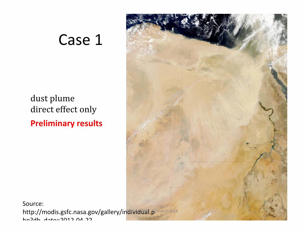
Case 1: Dust storm over Egypt (18 April 2012)

Experiment set‐up• Aerosol effects: forecast with and without interactive aerosols,

limited to direct effect only. Each participant defines if the aerosols fields will be climatological or prognostic.

• Duration and time period: 10 days, April 13‐23 2012.

• Length: 10 days forecasts from the 00UTC or 1200UTC analysis with and without interactive aerosols.

• Center of the model domain (for limited area models): 300 E, 250 N

• Model configuration should be compatible with the configuration of the operational system used currently for NWP.

• Initial and boundary conditions for meteo fields can be provided upon demand by ECMWF (eg MACC fields including aerosols) for the limited area models.

Figure 1. The dust storm case (source: http://modis.gsfc.nasa.gov/gallery/individual.php?db_date=2012‐04‐2229th‐WGNE ‐ 13march2014

Case 1: Model evaluation and Protocols


Case 2: Extreme pollution in Beijing (12‐16 January 2013)


includingdirectandindirecteffects.• Ideallyfourexperimentsshouldbeperformed:

• Duration and time period: 14 days, from January 7 to January 21 2012• Length: 10 days forecasts from the 00UTC or 1200UTC analysis with

and without interactive aerosols. • Center of the model domain (for limited area models): 1160 E, 400 N• Model configuration should be compatible with the configuration of

the operational system used currently for NWP. • Initial and boundary conditions for meteo fields will be provided upon

demand by ECMWF (eg MACC) for the limited area models.

Figure 2. Picture of a hazy day in Beijing, China, January 14, 2013 (Source: http://news.yahoo.com/photos/china‐s‐air‐pollution‐problem‐slideshow/).


Case 3: Persistent biomass burning smoke in Brazil –the SAMBBA case


includingdirectandindirecteffects.• Ideallyfourexperimentsshouldbeperformed:

• Duration and time period: 10 days, 05‐15 September 2012• Length: minimum of 3 days forecasts from the 00UTC or 1200UTC

analysis with and without interactive aerosols. • Center of the model domain (for limited area models): 600 W, 100 S• Model configuration should be compatible with the configuration of

the operational system used currently for NWP. • Initial and boundary conditions for meteo fields can be provided upon

by ECMWF (eg MACC) for the limited area models.

Figure 3. Up: Fire counts location and accumulated for September 2012 (source:http://www.inpe.br/queimadas/). Down: Monthly average of aerosol optical depth at 550 nm from MODIS for September 2012 (source: http://disc.sci.gsfc.nasa.gov/giovanni). The dots with the initials RB, PV, … denote AERONET site locations.


Participants


X = data not yet available for processing or analyzed

Centersparticipantsandageneraldescriptionoftheirmodelingsystems**


** Appendix 3 contains more detailed information.

Centersparticipantsandageneraldescriptionoftheirmodelingsystems:

GlobalScale

• NASA/Goddard – GEOS‐5 with GOCART aerosol model.– GOCART bulk model for dust, sea‐salt, sulfates, carbonaceous– Global, 25 km, 72 levels, top at 0.01hPa

• JMA– MASINGAR mk‐2 aerosol model + MRI‐AGCM3 (dynamics)– 2‐moment bulk cloud model w/ explicit aerosol effects– Interactive components: sulfate, BC, organics, sea‐salt and dust.– Prescribed emissions from MACCity and GFAS 1.0– Global TL319L40, top at 0.4 hPa

• NCEP– NOAA/NCEP Global Forecast System (GFS)– Radiation based on Rapid Radiative Transfer Models (RRTM)– A climatological aerosol distribution at 5° resolution (Hess et al., 1998)– Only consider direct radiative effect.– Global model T574L64, top at 0.32 hPa.

Centersparticipantsandageneraldescriptionoftheirmodelingsystems:

LimitedAreaModels

• Meteo‐France and Met. Service of Algeria– ALADIN LAM coupled with Dust Entrainment and Deposition (DEAD) model. – Dust transport and optical properties are calculated using the three‐moment Organic

Inorganic Log‐normal Aerosol Model (ORILAM) (Tulet et al. 2005)– Radiation RRTM for LW and FMR for SW.– Only direct effect. – Resolution 7.5 x 7.5 km and 70 levels– IC/BC from ARPEGE global model. – Case 1 only.

• CPTEC/Brazil– BRAMS LAM coupled with the CCATT aerosol‐chemistry model.– Focus on biomass burning aerosol (Case 3)– Brazilian biomass burning emission model coupled with an interactive plumerise model– Direct effect using CARMA radiation parameterization– Indirect effect included at 2‐moment bulk cloud scheme (under development)– Indirect effect included at cumulus convection scheme – Resolution: 10 x 10 km, 50 levels– IC/BC from GFS + MACC

• To be completed with – ECMWF model– Barcelona Supercomputer Ctr. model– WRF/Chem at NOAA– …

Case 1

dustplumedirecteffectonly

Source: http://modis.gsfc.nasa.gov/gallery/individual.php?db date=2012‐04‐22


Preliminary results

MISR and MODIS AOD (550nm) 18apr2012

Source: Giovanni /NASA

1.5

0.6

0.5

>2


~ 1.


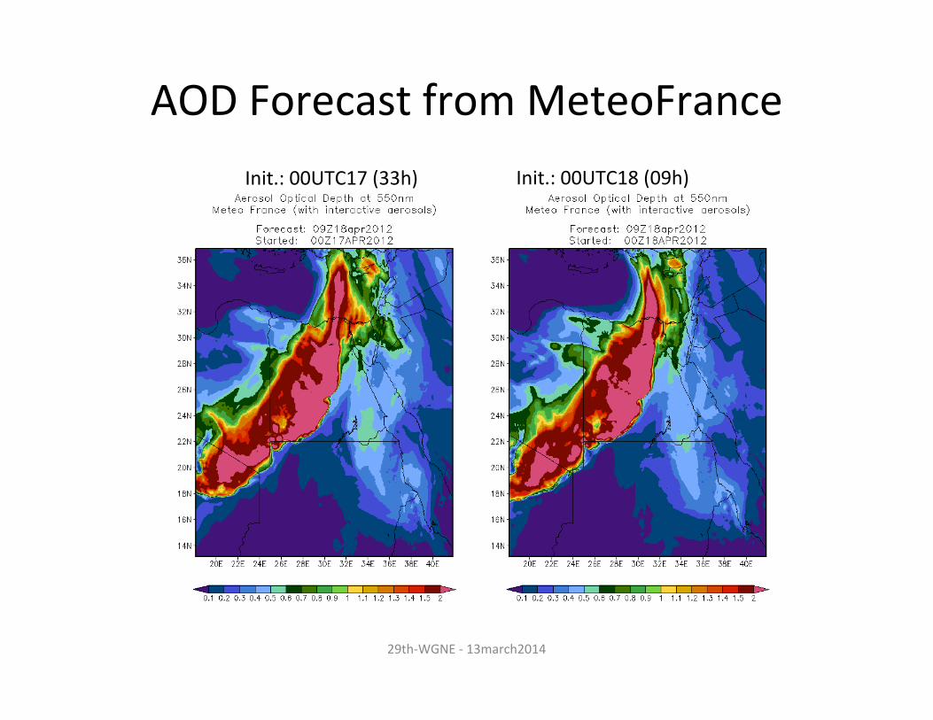
CASE 1 – DUSTJMA and NASA AOD (550 nm) FCT

AOD Forecast from JMA09UTC18Apr2012

Init.: 00UTC16 (57h) Init.: 00UTC17 (33h) Init.: 00UTC18 (09h)


AOD Forecast from NASA


Init.: 00UTC16 (57h) Init.: 00UTC17 (33h) Init.: 00UTC18 (09h)

AOD Forecast from MeteoFrance


Init.: 00UTC17 (33h) Init.: 00UTC18 (09h)

Climatological AOD from NCEP


AOD at 550nm

Inter‐comparison


NCEP JMA

NASA MeteoFrance

• NCEP : climatology does not capture the strong event (as expected).

• JMA/NASA/MF have similar pattern in terms of spatial distribution.

• AOD values : MF > JMA > NASA

Column Integrated mass of dust:Inter‐comparison


JMA

JMA

NASA MeteoFrance

1. Large differences on the dust mass: from 20 g/m2 JMA for max 4 g/m2 NASA2. MeteoFrance: we need to check the units3. NCEP does not have this prognostic

Impacts on weather forecasting

• Radiativeshortwavefluxatsurface• Airtemperatureat2m• Windmagnitudeat10m


Rad. short wave at surface from JMAInit: 00Z17APRIL – Fct: 09Z18APRIL (33h)


(W m‐2)

Rad SW with aer Rad SW (aer) – (no‐aer)

Location of the plume

Weak effect?

Large AOD but a weak effect? RAD SW: (aer) – (no‐aer) is not large as should be expected

evaluating aerosols impacts on numerical weather prediction · evaluating aerosols impacts on...

Documents