evaluating aquacrop model to improve crop water ... · evaluating aquacrop model to improve crop...

Available online at www.pelagiaresearchlibrary.com

Pelagia Research Library

Advances in Applied Science Research, 2014, 5(5):293-304

ISSN: 0976-8610 CODEN (USA): AASRFC

293 Pelagia Research Library

Evaluating AquaCrop model to improve crop water productivity at North Delta soils, Egypt

Ahmed M. Saad*, Marwa G. Mohamed and Gamal A. El-Sanat

Agriculture Research Center, Soil, Water and Environment Research Institute, Soil improvement

and Conservation Department, 9 Cairo University Street, Giza, Egypt _____________________________________________________________________________________________

ABSTRACT AquaCrop model (version 4) was validated using data from two field experiments conducted at North Delta (Sakha and El-Hamoul Districts) during the summer seasons of 2012 and 2013. Maize cross 321 variety was sown to study the effect of deficit irrigation, nitrogen fertilization and soil mulching on maize water productivity. After that, AquaCrop model was validated using such data by different statistical indicators such as coefficient of determination( R2),normalized root mean square error ( NRMSE),degree of agreement (D )and efficiency (E). Results indicated that, AquaCrop software was able to simulate well maize water productivity under different irrigation regimes, nitrogen fertilization levels and mulching application at North Delta. Where, under non saline soil conditions (Sakha location) values of R2, NRMSE, D and E were 0.88, 0.36, 0.98 and 0.99 % respectively. While, under saline soil conditions ( El-Hamoul location) values were 0.88, 15.5, 0.12 and 0.77 % for R2, NRMSE, D and E respectively. Data also, showed that, under non saline soil, the highest value of water productivity was obtained by irrigation at 36 days after post planting irrigation ,then irrigation at 70 % depletion from soil available water, non limiting nitrogen fertilization and adding plastic mulching. While, under saline soil conditions, irrigation at 26 days after post planting irrigation, then irrigation at 50 % depletion from soil available water, near optimal nitrogen fertilization and plastic mulching gave the best value of water productivity. Key words: Deficit irrigation, Model, Mulching, Statistical indicators ,Validation _____________________________________________________________________________________________

INTRODUCTION

There are an urgent need to increase crop water productivity (WP), due to the sharp declining in water resources allocated to agriculture and continuing population increase [1]. This should include the employment of techniques and practices that deliver a more accurate supply of water to crops. Furthermore, there is a need to quantify the impact of the water limitation on crop productivity. Therefore, the necessity to develop a crop simulation models was arisen to use the existing knowledge of yield responses to water supply and quantify that in term of yield losses. Nitrogen fertilization plays a key role in plant growth, yield and hence crop water productivity. This nutrient element is recognized in maize production as the first major nutrient that begins to limit normal plant growth. It has received more study and attention than any other nutrient. Mulch is usually applied towards the beginning of the growing season, and is often reapplied as necessary. It serves initially to warm the soil helping it retain heat which is lost during the night. This allows early seedling of cereal crops and encourages faster growth. As the season progress, mulch stabilizes the soil temperature and moisture, and prevents sunlight from germinating weed seeds [2]. Maize is one of the most widely consumed cereal crops grown worldwide under different environmental conditions. The growing global population puts more strain for increased cereal production in the next decades to feed this population which greatly drive the global water demand for different purposes. Meanwhile humankind has to cope with the predicted impacts of future climate change on water resources availability especially in the arid and semi-arid regions. Irrigated agriculture is hence under high pressure to increase the water use efficiency during these

Ahmed M. Saad et al Adv. Appl. Sci. Res., 2014, 5(5):293-304 _____________________________________________________________________________


conditions. For this purpose several techniques and models have been developed to simulate the current and future scenarios for future planning and management of the water resources. AquaCrop is among such models which reliably simulate achievable yields of major crops as a function of water consumption under rainfed, supplemental, deficit, and full irrigation conditions, with comparatively less data demand [3]. The first crop chosen to parameterize and test the new FAO AquaCrop model was maize [4]. Also, it was used for growth simulation of cotton [5], sunflower [3], barley, [6], and Teff (Eragrostis tef), under different water regimes. The results of these experiments showed that the AquaCrop model can be used to explore management options and improve water productivity. AquaCrop has been developed to provide an easy – to –use modeling tool to an ample range of users ( farmers, agricultural consultants, water managers and policymakers) interested in attainable crop biomass and harvestable yield under different scenarios of water and nutrient input [3]. The model focuses on water input as the most limiting factor of crop growth, especially in arid and semi arid regions where water stress varies in intensity, duration, and time of occurrence [7], [8]. AquaCrop has a simple, user friendly structure, and employs 33 crop input parameters that can be observed easily in the field; for example, the percentage of canopy cover instead of leaf area index (LAI) and other biomass –related physiological inputs; numerical and/ or descriptive characterization of crop water stress tolerance, soil texture, and nutrient input. In fact, it is expected that this simple structure and reduced number of parameters could facilitate model calibration and utilization for different crops and under different management strategies. Notwithstanding the reduction and simplification of the input variables, the model maintains a significant number of main output data, including the simulation of canopy cover, biomass and soil water components over the whole growing cycle, and the final harvestable yield [3] ,[9].Therefore, the objectives of this study could be summarized as follows: (1): Evaluating AquaCrop model (version 4) under Egyptian soil conditions; (2): Improving crop water productivity under different treatments such as, irrigation regime, soil mulching, nitrogen fertilization and soil salinity.

MATERIALS AND METHODS

2.1. Sites and climate of the experimental field: The experiments were conducted on 2012 and 2013 at two experimental fields of North Delta (Egypt), Kafr El-Sheikh Governorate ( Sakha and El-Hamoul). The first experimental field was located in Sakha District ( non saline soil), 31º 03 latitude, and 30º 57 longitude. While, the second experimental field was conducted in El-Hamoul District represent saline soil , 31º 18 N and 31º 75 E. Soil texture was clay in both fields of experiment. Values of field capacity were 40.8 % and 41.8 % for both non saline and saline soil respectively. Also, permanent wilting point percentages were 20.3 and 21.2 % for non saline and saline soil respectively. The area is characterized by a typical Mediterranean climate, with a hot and dry summer season. Weather data, including daily values of air temperature and humidity, wind speed and sunshine were collected at the agro meteorological station of Sakha agriculture research station, located about 50 m from Sakha location and 3000 m from El-Hamoul location. Data in (Table 1) show the climatic data in such locations during the summer seasons of 2012 and 2013.

Table 1: Main values of meteorological data during maize growing seasons 2012 and 2013

Months Mean temperature, Cº Relative humidity, % Wind speed, km day-1 Sunshine, hours May 25.7 61.38 240 11.0 June 29.3 68.3 207 12.5 July 29.1 71.19 180 12.3

August 28.0 69.58 170 11.5 September 25.8 66.30 175 10.4

Some properties of the studied soils before cultivation are shown in Table.2. 2.2. Cultural practices and basic treatments: Pure maize (Zea Mays,L.) cross hybrid 321 variety was planted with cropping density 5.0 plants per m2 in May 2012 and 2013 and harvested around september for both field experiments. Weeds were controlled by integrated weed management strategies that were standard of the region. The experiments, set according to a randomized block design with three replicates, including the following treatments: (1): Withholding in irrigation intervals after post planting irrigation by (15,26 and 36 days), only for the first irrigate after post planting irrigation.,(2): Irrigation at different levels of depletion from soil available water by D1 (30 %), D2 (50%) and D3 (70%) through all over the season after previous withholding intervals., (3): Four levels of nitrogen fertilization N1 (non limiting), N2 ( near optimal), N3 (moderate), and N4 (poor)., (4): Two types of soil mulching i.e (plastic mulching and organic mulching).



Table 2: Some physical and chemical properties of the studied soils before cultivation

Soil properties Normal soil Saline soil

Ph

ysic

al p

rope

rtie

s Sand % 16.9 16.56 Silt % 26.5 23.64 Clay % 56.5 59.8 Soil texture clay clay Field capacity,% 40.8 41.8 Wilting point, % 20.3 21.2 Bulk density,Mg m-3 1.24 1.38 Organic matter, % 1.85 1.55

Che

mic

al p

rop

ert

ies

CaCO3, % 2.45 4.4 pH* 7.65 8.0 EC **, dS m-1 1.88 5.6 Ca++ meq l-1 3.72 13.0 Mg++ meq l-1 2.08 12.3 Na+ meq l-1 12.8 30.1 K+ meq l-1 0.20 0.6 CO3

-- meq l-1 0.00 0.0 HCO3

- meq l-1 5.4 4.0 CL- meq l-1 8.90 22.7 SO4-- meq l-1 4.5 29.3 Available Nitrogen, mgkg-1 50.6 30.1 Available phosphorus. mgkg-1 16.3 10.0 Available potassium,mgkg-1 489.5 650

* pH was determined in soil: water suspension (1:2.5). ** EC was determined in soil paste extract.

2.3. Description of AquaCrop model: AquaCrop is a new water-driven crop growth model [3],[9]. The biomass growth rate is linearly proportional to transpiration through the following equation: AGB = WP × Tc/ET° here AGB is the aboveground biomass rate; WP is the water productivity (biomass per unit of accumulated water transpired); Tc is the crop transpiration; and ETº is the reference evapotranspiration,used to normalize Tc .

Soil water balance is performed on a daily basis including the processes of ifiltration, runoff, deep percolation, crop uptake, evaporation, transpiration, and capillary rise. The model keeps track of the rainfall and irrigation, and seperates evaporation from transpiration through the percentage of canopy cover as described in detail by [9]. AquaCrop does not calculate ETº , and it is one of the weather inputs in the model. In this study, ETº data were estimated from the nearby meteorological station using the FAO Penman-Monteith approach. AquaCrop relates its soil-crop- atmosphere components through its soil and its water balance, the atmosphere (rainfall, temperature, evapotranspiration, and carbon dioxide concentration) and crop conditions ( phenology,crop cover, root depth, biomass production and harvestable yield) and field management (irrigation, fertility and field agronomic practices) components [9],[3]. 2.4. Methods of model validation and evaluation: The model validations were based on the comparison between simulated (predicted) and observed (measured) data for all treatments. In particular, the following crop growth parameters were analyzed: (I): maize grain yield, and (II): maize water productivity. For such aim,several statistical indicators are available to evaluate the performance of a model [10]. Each has its own strengths and weaknesses, which means that the use of an ensemble of different indicators is necessary to sufficiently assess the performance of the model [11]and[12]. In the equations, Oi and Pi are the observations and predictions respectively, and their averages and n the number of observations. 1- Coefficient of determination (R2): The coefficient of determination r² is defined as the squared value of the pearson correlation coefficient. R² signifies the proportion of the variance in measured data explained by the model, or can also be interpreted as the squared ratio between covariance and the multiplied standard deviations of the observations and predictions. It ranges from 0 to 1, with values close to 1 indicating a good agreement, and typically values greater than 0.5 are considered acceptable in watershed simulations [13].

Ahmed M. Saad et al _____________________________________________________________________________

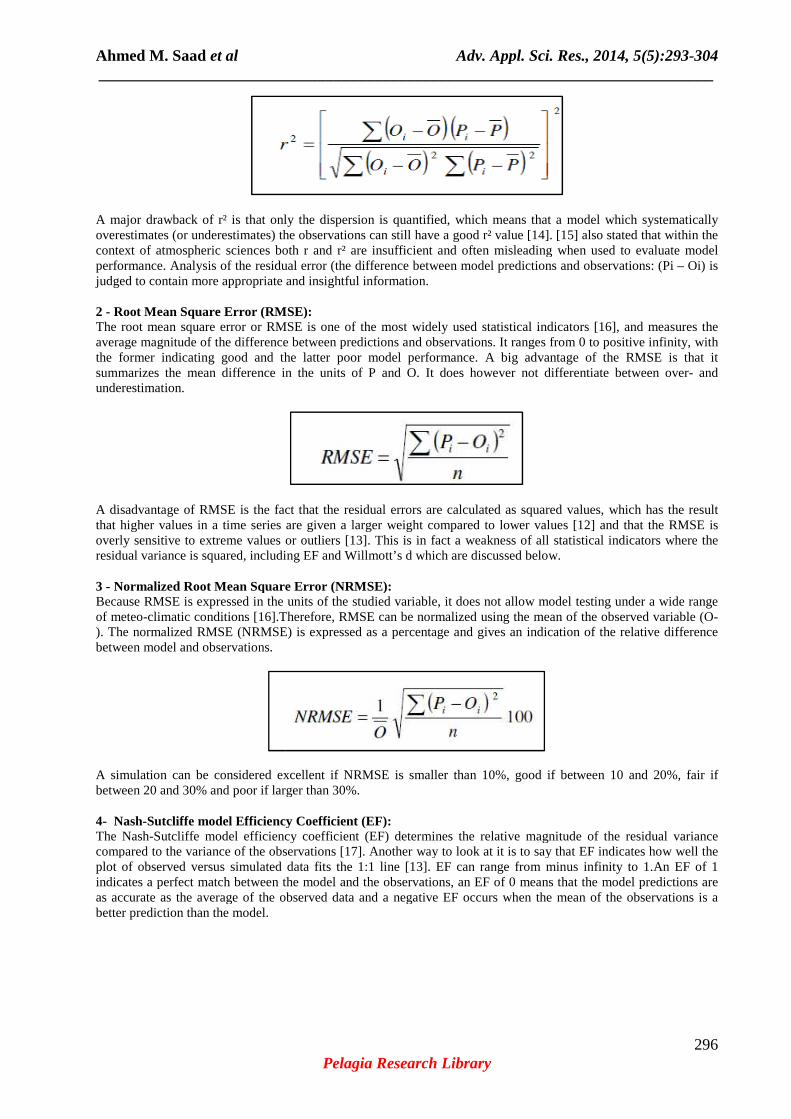
A major drawback of r² is that only the dispersion is quantified, which means that a model which systematically overestimates (or underestimates) the observations can still have a good r² value context of atmospheric sciences both r and r² are insufficient and often misleading when used to evaluate model performance. Analysis of the residual error (the difference between model predictions and observations: (Pi judged to contain more appropriate and insightful in 2 - Root Mean Square Error (RMSE):The root mean square error or RMSE is one of the most widely used statistical indicators average magnitude of the difference between predictions and observations. It ranges from 0 to the former indicating good and the latter poor model performance. A big advantage of the RMSE is that it summarizes the mean difference in the units of P and O. It does however not differentiate between overunderestimation.

A disadvantage of RMSE is the fact that the residual errors are calculated as squared values, which has the result that higher values in a time series are given a larger weight compared to lower values overly sensitive to extreme values or outliersresidual variance is squared, including EF and Willmott’s d which are discussed below. 3 - Normalized Root Mean Square Error (NRMSE):Because RMSE is expressed in the units of the studied variable, it does not allow model testing under a wide range of meteo-climatic conditions [16].Therefore, RMSE can be normalized using the mean of the observed variable (O). The normalized RMSE (NRMSE)between model and observations.

A simulation can be considered excellent if NRMSE is smaller than 10%, good if between 10 and 20%, fair if between 20 and 30% and poor if larger than 30%. 4- Nash-Sutcliffe model Efficiency The Nash-Sutcliffe model efficiency coefficient (EF) determines the relative magnitude of the residual variance compared to the variance of the observations plot of observed versus simulated data fits the 1:1 line indicates a perfect match between the model and the observations, an EF of as accurate as the average of the observed data and a negative EF occurs when the mean of the observations is a better prediction than the model.

Adv. Appl. Sci. Res., 2014, 5(5):_____________________________________________________________________________

Pelagia Research Library

major drawback of r² is that only the dispersion is quantified, which means that a model which systematically overestimates (or underestimates) the observations can still have a good r² value [14]. [15

iences both r and r² are insufficient and often misleading when used to evaluate model performance. Analysis of the residual error (the difference between model predictions and observations: (Pi judged to contain more appropriate and insightful information.

Root Mean Square Error (RMSE): The root mean square error or RMSE is one of the most widely used statistical indicators average magnitude of the difference between predictions and observations. It ranges from 0 to the former indicating good and the latter poor model performance. A big advantage of the RMSE is that it summarizes the mean difference in the units of P and O. It does however not differentiate between over

A disadvantage of RMSE is the fact that the residual errors are calculated as squared values, which has the result that higher values in a time series are given a larger weight compared to lower values

e values or outliers [13]. This is in fact a weakness of all statistical indicators where the residual variance is squared, including EF and Willmott’s d which are discussed below.

Normalized Root Mean Square Error (NRMSE): Because RMSE is expressed in the units of the studied variable, it does not allow model testing under a wide range

.Therefore, RMSE can be normalized using the mean of the observed variable (O). The normalized RMSE (NRMSE) is expressed as a percentage and gives an indication of the

A simulation can be considered excellent if NRMSE is smaller than 10%, good if between 10 and 20%, fair if arger than 30%.

fficiency Coefficient (EF): Sutcliffe model efficiency coefficient (EF) determines the relative magnitude of the residual variance

compared to the variance of the observations [17]. Another way to look at it is to say that EF indicates how well the plot of observed versus simulated data fits the 1:1 line [13]. EF can range from minus infinity to 1.An EF of 1 indicates a perfect match between the model and the observations, an EF of 0 means that the model predictions are as accurate as the average of the observed data and a negative EF occurs when the mean of the observations is a

Adv. Appl. Sci. Res., 2014, 5(5):293-304 _____________________________________________________________________________

296

major drawback of r² is that only the dispersion is quantified, which means that a model which systematically [15] also stated that within the

iences both r and r² are insufficient and often misleading when used to evaluate model performance. Analysis of the residual error (the difference between model predictions and observations: (Pi – Oi) is

The root mean square error or RMSE is one of the most widely used statistical indicators [16], and measures the average magnitude of the difference between predictions and observations. It ranges from 0 to positive infinity, with the former indicating good and the latter poor model performance. A big advantage of the RMSE is that it summarizes the mean difference in the units of P and O. It does however not differentiate between over- and

A disadvantage of RMSE is the fact that the residual errors are calculated as squared values, which has the result that higher values in a time series are given a larger weight compared to lower values [12] and that the RMSE is

. This is in fact a weakness of all statistical indicators where the

Because RMSE is expressed in the units of the studied variable, it does not allow model testing under a wide range .Therefore, RMSE can be normalized using the mean of the observed variable (O-

is expressed as a percentage and gives an indication of the relative difference

A simulation can be considered excellent if NRMSE is smaller than 10%, good if between 10 and 20%, fair if

Sutcliffe model efficiency coefficient (EF) determines the relative magnitude of the residual variance . Another way to look at it is to say that EF indicates how well the

. EF can range from minus infinity to 1.An EF of 1 0 means that the model predictions are

as accurate as the average of the observed data and a negative EF occurs when the mean of the observations is a



EF is very commonly used, which means that there is a large number of reported values available in literature [13]. However, like r², EF is not very sensitive to systematic over- or underestimations by the model [14]. 5 - Willmott’s index of agreement (d) : The index of agreement was proposed by [15] to measure the degree to which the observed data are approached by the predicted data. It represents the ratio between the mean square error and the “potential error”, which is defined as the sum of the squared absolute values of the distances from the predicted values to the mean observed value and distances from the observed values to the mean observed value [11]. It overcomes the insensitivity of r² and EF to systematic over- or underestimations by the model [12], [11]. It ranges between 0 and 1, with 0 indicating no agreement and 1 indicating a perfect agreement between the predicted and observed data.

A disadvantages of d is that relatively high values may be obtained (over 0.65) even when the model performs poorly, and that despite the intentions of [15] d is still not very sensitive to systemic over- or underestimations [14].

RESULTS AND DISCUSSION

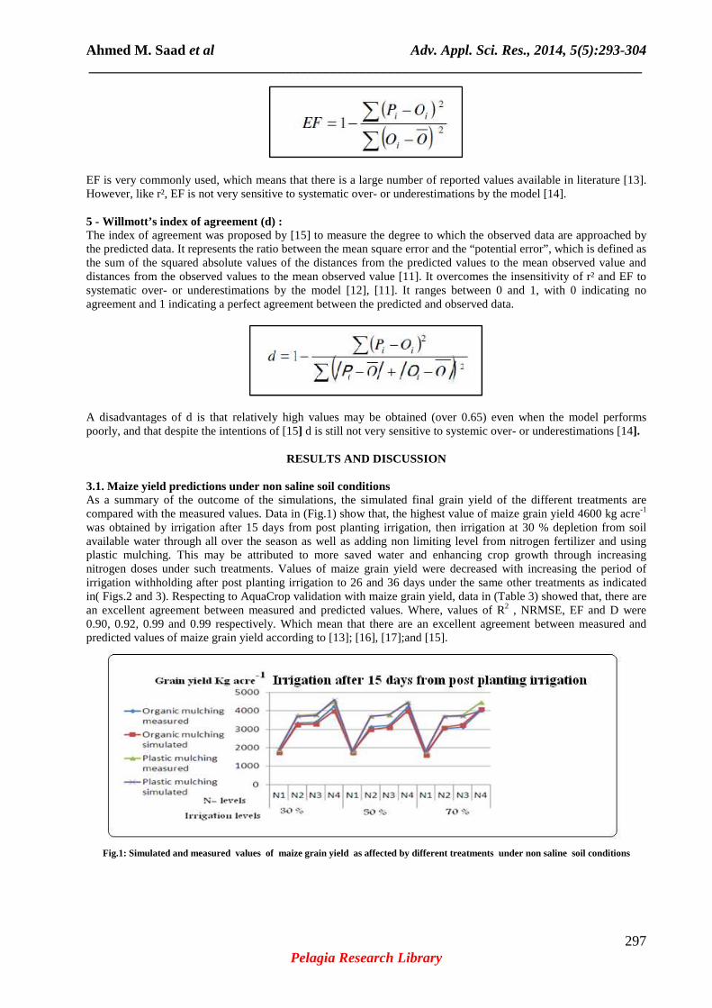
3.1. Maize yield predictions under non saline soil conditions As a summary of the outcome of the simulations, the simulated final grain yield of the different treatments are compared with the measured values. Data in (Fig.1) show that, the highest value of maize grain yield 4600 kg acre-1 was obtained by irrigation after 15 days from post planting irrigation, then irrigation at 30 % depletion from soil available water through all over the season as well as adding non limiting level from nitrogen fertilizer and using plastic mulching. This may be attributed to more saved water and enhancing crop growth through increasing nitrogen doses under such treatments. Values of maize grain yield were decreased with increasing the period of irrigation withholding after post planting irrigation to 26 and 36 days under the same other treatments as indicated in( Figs.2 and 3). Respecting to AquaCrop validation with maize grain yield, data in (Table 3) showed that, there are an excellent agreement between measured and predicted values. Where, values of R2 , NRMSE, EF and D were 0.90, 0.92, 0.99 and 0.99 respectively. Which mean that there are an excellent agreement between measured and predicted values of maize grain yield according to [13]; [16], [17];and [15].

Fig.1: Simulated and measured values of maize grain yield as affected by different treatments under non saline soil conditions





Table 3: Evaluating AquaCrop model with maize grain yield under different treatments in non saline soil conditions

Statistical indicators

Treatments Elapsed time after post

planting irrigation Irrigation at different levels of

depletion from soil available water Nitrogen fertilization

levels Soil

mulching 15 days 30 % Non limiting Plastic 26 days 50 % Near optimal Organic 36 days 70 % Moderate

Poor R2 0.90

NRMSE 0.92 EF 0.99 D 0.99

3.2. Maize water productivity prediction under non saline soil conditions As shown in (Figs 4,5 and 6), values of WP were increased with using plastic mulching, level of non limiting nitrogen fertilizer, and application of deficit irrigation. Where, the highest predicted value of WP 2.10 kg m-3 was obtained by irrigation after 36 days from post planting irrigation then irrigation at 70 % depletion from soil available water, as well as adding level of non limiting nitrogen fertilizer and using plastic mulching as compared to other treatments. Such increase in WP may be due to the following reasons: 1. Water loss through evaporation is reduced due to using plastic mulching. 2. The negative effect of drought stress during specific phonological stages on biomass partitioning between reproductive and vegetative biomass (harvest index [18], [19]and [20] is avoided, which stabilizes or increases the number of reproductive organs and/or the individual mass or reproductive organs (filling) [21].



3. WP for the net assimilation of biomass as follow:

With biomass in the numerator and with ETa in the denominator is increased as drought stress is mitigated or crops become more hardened. This effect is thought to be rather limited given the conservative behavior or biomass growth in response to transpiration [22]and[23]. 4. WP for the net assimilation of biomass is increased due to the synergy between irrigation and fertilization [24]. This includes cases where irrigation is reduced if fertilizer levels and native fertility are low [ 25]. 5. Negative agronomic conditions are avoided during crop growth, such as pests, diseases, anaerobic conditions in the root zone due to water logging, etc. [26]and [25]. Data in (Table 4) showed an excellent agreement between measured and predicted values of WP under different treatments. Where, R2 value was 0.88 which achieve a good agreement according to [13], NRMSE value was less than 10 %, values of EF and D were 0.98 and 0.99 respectively. Therefore, AquaCrop model was able to simulate maize water productivity under non saline soil conditions.

Fig.4: Simulated and measured values of maize water productivity as affected by different treatments under non saline soil conditions





Table 4: Evaluating AquaCrop model with maize water productivity under different treatments in non saline soil conditions





levels Soil


Poor R2 0.88

NRMSE 0.36 EF 0.98 D 0.99

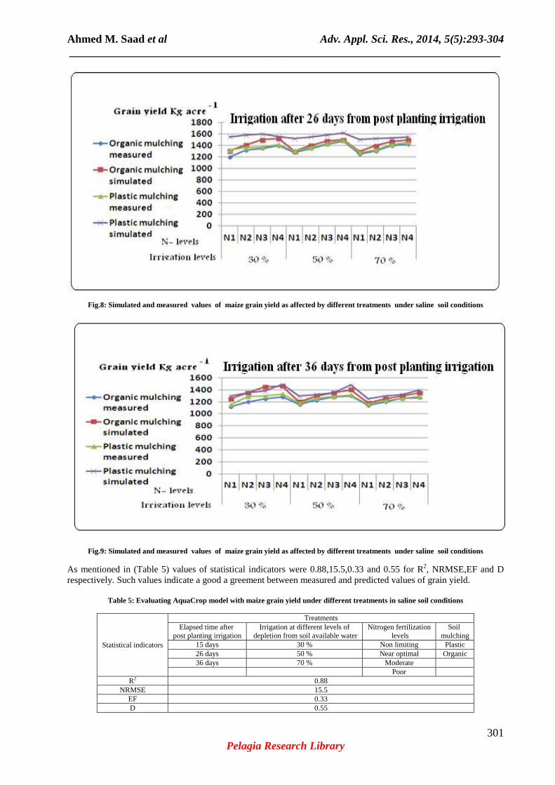
3.3. Prediction of maize grain yield under saline soil conditions AquaCrop model (version 4) uses the calculation procedure presented in Budget [27], [28],[29]and[30] to simulate salt movement and retention in the soil profile. The highest predicted value of maize grain yield under salinity conditions 1700 kg acre-1 was obtained by irrigation after 15 days from post planting irrigation followed by irrigation at 30 % depletion from soil available water as well as using plastic mulching and level of non limiting from nitrogen fertilizer, as shown in (Fig.7). Values of maize grain yield were decreased with increasing the period of irrigation intervals after post planting irrigation as indicated in (Figs.8 and 9).

Fig.7: Simulated and measured values of maize grain yield as affected by different treatments under saline soil conditions





As mentioned in (Table 5) values of statistical indicators were 0.88,15.5,0.33 and 0.55 for R2, NRMSE,EF and D respectively. Such values indicate a good a greement between measured and predicted values of grain yield.

Table 5: Evaluating AquaCrop model with maize grain yield under different treatments in saline soil conditions


Treatments Elapsed time after

post planting irrigation Irrigation at different levels of


levels Soil


Poor R2 0.88

NRMSE 15.5 EF 0.33 D 0.55



3.4. Prediction of maize water productivity under saline soil conditions Values of WP were increased due to increasing nitrogen fertilization, proper irrigation management and using plastic mulching as shown in (Figs.10,11 and 12). Where, the highest value of WP 0.78 kg m-3 was obtained by irrigation after 26 days from post planting irrigation followed by irrigation at 50 % depletion from soil available water in addition to using plastic mulching and adding level of non limiting from nitrogen fertilizer. Respecting to AquaCrop evaluation under this condition. Data presented in (Table 6) report that, there are a good agreement between measured and predicted values of WP. Where, values of R2, NRMSE,EF and D were 0.88, 15.5, 0.12 and 0.77 respectively. Therefore, AquaCrop model could be used adequately under these conditions to predict crop water productivity with different treatments like irrigation, fertilization and field practice management.

Fig.10: Simulated and measured values of maize water productivity as affected by different treatments under saline soil conditions


Table 6: Evaluating AquaCrop model with maize water productivity under different treatments in saline soil conditions





levels Soil


Poor R2 0.88

NRMSE 15.5 EF 0.12 D 0.77




CONCLUSION

AquaCrop software (version,4) was able to simulate well grain yield and water productivity of maize crop under different treatments such as irrigation regimes, nitrogen fertilization, soil salinity and soil mulching at North delta soils (Egypt). Therefore, this model can be used as a decision support tool in increasing water productivity by project managers, consultants, irrigation engineers and farmers. In other words, this model can be used to simulate the water management effects on yield and handle managements that increase water productivity. Also, the highest value of maize water productivity was achieved by irrigation after 36 days post planting irrigation, then irrigation at 70 % depletion from soil available water as well as applying both non limiting nitrogen fertilizer and plastic mulching, under non saline soil conditions. While, under saline soil conditions, the highest value of crop water productivity was obtained by irrigation after 26 days from post planting irrigation then irrigation at 50 % depletion from soil available water through season in addition to adding moderate nitrogen fertilizer and plastic mulching. Acknowledgments This research has been undertaken with the support and collaboration from a wide range of individuals and institutions. I would like to express my sincere thanks to especially to Prof.Dr. Pasquale Steduto (FAO, land and water division, Rome, Italy) the essential member of AquaCrop preparing team , who supported me with many updated information of AquaCrop (version 4). Research funded by Agriculture Research Center, Egypt and carried out in North Delta region (Kafr El-Sheikh Governorate), Egypt.

REFERENCES

[1] Kijne, J.W., Barker, R., Molden, D. Water Productivity in Agriculture: Limits and Opportunities for Improvement, Comprehensive Assessment of Water Management in Agriculture Series, No. 1 International Water Management Institute, Srilanka, 2003. [2] Louise; B. B., James, B. America`s garden book, New York, Macmillan USA, P.768, 1996. [3] Steduto, P., Hsiao,T.C., Raes,D., Fereres, E. Aquacrop. Agron. J. 2009, 101: 426-437. [4] Hsiao, T. C., Heng ,L., Steduto,P., Rojas – lara, R ., Ferese,E. Agron. J., 2009, 101( 3): 448 – 459. [5] Farahani, H., Izzi, G., Oweis,T. Y. Agron. J., 2009, 101:469–476. [6] Araya, A., Solomon,H., Kiros, M. H., Afewerk, K., Taddese, D. Ann. Rev. Plant Physiol., 1973, 24: 519-570. [8] Bradford, K.J., Hsiao, T.C. Physiological responses to moderate water stress. In OL Lange, PS Nobel, CB Osmond, H Ziegler, eds, Encyclopedia of Plant Physiology, New Series, Vol 12b. Springer Verlag, New York, 1982, pp 263-324. [9] Raes, D., Steduto,P., Hsiao, T.C., Fereres,E. Agron. J., 2009, 101:438–447. [10] Loague, K., Green,R.E. J. Cantam. Hydrol., 1991, 7: 51-73. [11] Willmott, C. J. On the evaluation of model performance in physical geography. In Spatial Statistics and Models, Gaile GL, Willmott CJ (eds). D. Reidel: Boston. 443–460, 1984. [12] Legates, D. R., McCabe, G. J. Water Resources Research, 1999, 35, 233–241. [13] Moriasi, D. N., Arnold, J. G., Liew, M. W. V., Bingner, R. L., Harmel ,R. D., Veith,T. L. Transactions Of The ASABE, 2007, 50, 885–900. [14] Krause, P., Boyle, D. P., Bäse, F. Advances In Geosciences, 2005, 89–97.



[15] Willmott, C. J. Bulletin American Meteorological Society 63, 1309–1313, 1982. [16] Jacovides, C. P., Kontoyiannis, H. Agricu Water Manag. J, 1995: 27, 365–371. [17] Nash, J.E., Sutcliffe,J.V. J. Hydrol., 1970, 10: 282–290. [18] Fereres, E., Soriano, M. A. J. Exp. Bot., 2007, 58: 147-159. [19] Hsiao,T.C., Steduto,P., Fereres,E. Irrigate.Sci., 2007, 25,209-231. [20] Reynolds , M., Tuberosa, R. Current opinion in plant Biology, 2008,11: 171-179. [21] Karam,F., Kabalan,R., Briedi,J., Rouphael,Y., Oweis, T. Agric . water Manag.,Elsiver, Netherlands , 2009,96(4):603 – 615. [22] De Wit, C.T. Transpiration and Crop Yields. Versl. Landbouwk. Onderz. 64.6Pudoc, Wageningen, 1958. [23] Steduto, P., Hsiao,T.C., Fereres,E. Irrig. Sci., 2007, 25: 189-207. [24] Steduto, P., Albrizio,R. Agric. For. Meteorol., 2005, 130: 269-281. [25] Geerts, S., Raes, D., Garcia,M., Vacher,J., Mamani,R., Mendoza,J., Huanca,R., Morales, B., Miranda, R., Cusicanqui, J., Eur. J. Agron., 2008, 28, 427–436. [26] Pereira ,L. S., Cordery, I., Lacovides, I. Technical Documents in Hydrology No.58, 2002. [27] Raes, D., Van Goidsenhoven, B., Goris,K., Samain B., De Pauw , E., El Baba , M., Tubail, K. , Ismael, J., De Nys,E. BUDGET, a management tool for assessing salt accumulation in the root zone under irrigation. In: A.A. soares and H.M. Saturnino (Editors) Environment-Water: Competitive Use and Conservation Strategies for Water and natural resources. International Commission on Irrigation and Drainage (ICID), Fortaleza, Brazil:244-252, 2001. [28] Raes, D. BUDGET, a soil water and salt balance model: reference manual. K.U.Leuven, Belgium, 80 pp, 2002. [29] De Nys, E, Raes,D., Le Gal, P.Y, Cordeiro,G., Speelman,S., J. of Irrig and Drain Eng, 2005, (131, 4): 351 – 357. [30] Raes, D., Geerts, S., Kipkorir, E., Wellens, J., and Sahli, A. Agricultural Water Management, 2006, 81(3): 335-357.