evaluating benefi t guarantees in social security benefi t guarantees in social security march...
TRANSCRIPT
Congressional Budget Offi ce
Background Paper
THE CONGRESS OF THE UNITED STATES
Evaluating Benefi t Guarantees inSocial Security
March 2006

Evaluating Benefit Guarantees inSocial Security:
A Background Paper
March 2006
CBO
The Congress of th
e United States O Congressional Budget Office
Note
Numbers in the tables and text of this paper may not sum to totals because ofrounding.

PrefaceSome proposals to modify the Social Security system by incorporating individual accounts would also require that beneficiaries receive a guaranteed minimum benefit, regardless of the accounts’ investment performance. The Congressional Budget Office (CBO) has developed the capacity to analyze the value of such guarantees and their potential cost to the government. This background paper demonstrates how benefit guarantees can be evaluated using two complementary approaches and discusses how to interpret the results. In keeping with CBO’s mandate to provide objective, nonpar-tisan analysis, the paper makes no policy recommendations.
Sven Sinclair, Deborah Lucas, Amy Rehder Harris, Michael Simpson, and Julie Topoleski prepared this paper under the supervision of Robert Dennis, Douglas Hamilton, John Sabelhaus, and Bruce Vavrichek. Wendy Kiska assisted with model development and computations. Paul Cullinan, Shinichi Nishiyama, Benjamin Page, and Marvin Phaup provided helpful comments, as did Kent Smetters of the Univer-sity of Pennsylvania. (The assistance of external reviewers implies no responsibility for the final product, which rests solely with CBO.)
Loretta Lettner edited the paper, and Christian Spoor proofread it. Maureen Costantino prepared the paper for publication. Lenny Skutnik produced the printed copies, and Annette Kalicki and Simone Thomas prepared the electronic version for CBO’s Web site (www.cbo.gov).
Donald B. MarronActing Director
March 2006

Contents
Introduction and Summary 1How Benefit Guarantees Would Work 1Approaches to Analyzing Benefit Guarantees 2Results of the Analysis 6
CBO’s Display of Risk in Social Security Proposals 6
Alternative Ways to Display the Risk Associated with Benefit Guarantees 7Estimating the Distribution of Future Payouts 9Estimating the Market Value of Guarantees 10
Guarantee Analysis in an Illustrative Proposal 12
Probabilities and Ranges of Outcomes 14
Market Values 16
Comparison of the Alternative Approaches 17
Conclusions 20
Appendix A: Options-Pricing Principles and the Discounting of RiskyCash Flows 23
Appendix B: Estimations of Guarantee Costs with 2 Percent Accounts 31
v

Tables
1.
Changes in the Present Value of Payments over a 75-YearHorizon for Illustrative Proposals with 4 Percent IndividualAccounts and Guarantees 17B-1.
Changes in the Present Value of Payments over a 75-YearHorizon for Illustrative Proposals with 2 Percent IndividualAccounts and Guarantees 32Figures
1.
Potential Distribution of Participants Receiving Guarantees on4 Percent Individual Accounts with a 100 Percent BenefitGuarantee 152.
Potential Distribution of Total Guarantee Outlays for 4 Percent Individual Accounts with a 100 Percent BenefitGuarantee 163.
Potential Distribution of Total Guarantee Outlays for4 Percent Individual Accounts with a 100 Percent BenefitGuarantee 184.
Potential Guarantee Costs for 4 Percent Individual Accountswith a 100 Percent Benefit Guarantee Under Two Approaches 195.
Potential Value of Guarantees on 4 Percent Individual Accountswith a 100 Percent Benefit Guarantee, 2000 Cohort, Across the Earnings Distribution 20A-1.
Values in Lattice Example 2 28Boxes
1.
What Would It Mean to Guarantee Benefits in Mandatory FederalPrograms? 42.
CBO’s Long-Term Model 8vi

Introduction and SummaryMany proposals to change Social Security include provisions that would introduce individual accounts to the program. Although the proposals differ in significant ways, they share one main feature: the amount of income available from an account at the beneficiary’s retirement would depend on contributions made to the account and the rate of return earned by assets held in the account, minus deductions for administra-tive costs.
The income from such accounts could be uncertain, which has sparked interest in having the government provide some sort of guarantees to participants. This Congres-sional Budget Office (CBO) background paper discusses methods for estimating the cost of such guarantees to the government.
How Benefit Guarantees Would WorkMany of the proposals that would introduce individual accounts would redirect a por-tion of Social Security payroll tax revenues to fully or partially finance the new ac-counts. To balance the resulting reduction in revenues, such proposals would typically reduce traditional Social Security benefits.1 Therefore, depending on the size of the benefit reduction and the investment performance of the account, an individual par-ticipant’s total benefit (the sum of the traditional benefit and income from the partic-ipant’s account) could be higher or lower than it would have been under the current system.
A number of the proposals would allow workers to invest a portion of the funds in their account in corporate stocks, typically through broadly diversified mutual funds. Proponents of individual accounts often emphasize the expected returns. Historically, stocks have yielded a higher rate of return than fixed-income securities, such as Trea-sury bonds. From 1926 to 2000, for example, the real (inflation-adjusted) rate of re-turn on large-company stocks averaged 7 percentage points more than the real rate of return on three-month Treasury bills.2 However, investments in stocks also carry cor-respondingly higher risks. According to historical data, over a period of 10 years, in-vestors face about a 25 percent chance of realizing lower returns from holding stocks in the Standard & Poor’s 500 than from holding 10-year Treasury notes.
Concerns about risk—especially if the introduction of individual accounts was ac-companied by a reduction in traditional benefits—have motivated discussions about providing some type of government-funded benefit guarantee for account holders. For example, the government might guarantee that the retirement income of workers
1. There are other reasons for reducing benefits, including efforts to improve the solvency of the Social Security system. Although some proposals combine solvency improvements with the intro-duction of individual accounts, those provisions are independent of each other. The analysis of guarantees in this paper does not depend on whether a given proposal would otherwise address the system’s solvency.
2. Congressional Budget Office, Social Security: A Primer (September 2001).
1
who participated in individual accounts was never less than the level of traditional benefits. If the accounts performed well enough to provide more than that guaranteed minimum, retirees would keep the gains; if the accounts did not reach that level, the government would make up the difference. Because the account holder would not face any risk of becoming worse off than he or she would be with traditional bene-fits—and could become better off—the average amount of income that the account holder could expect in retirement would be higher than what he or she would have otherwise received. In other words, the guarantee, on average, would represent an en-hancement of benefits.
Guarantees also could be designed in other ways. They could provide less-than-full protection, shielding the participants from only the worst outcomes. Or, instead of providing a minimum level of income (as in the first example), the government could guarantee a minimum rate of return on the assets in the accounts.
Despite their differences, the types of guarantees described above would all confer value to account holders by partially or fully protecting them from risk. In some cases, as previously noted, they would also provide a direct benefit enhancement. However, the increased benefits to account holders would create a corresponding cost for the federal government. Whenever an account fell short of promised benefits, the govern-ment—and, implicitly, taxpayers—would make up the difference. (Such a scenario would not imply a contractual obligation for the government; like other benefits, a system of guaranteed benefits could be altered by subsequent legislation. In its analysis of the value of guarantees and their future costs, however, CBO has assumed that the guarantees would be sustained. See Box 1 for a more detailed discussion of what guar-anteeing benefits in mandatory federal programs might entail.)
The net budgetary impact of a typical individual-account proposal with guarantees thus would involve three components: any change in the traditional Social Security defined benefit; any change in baseline tax revenues or outlays associated with fund-ing the accounts; and the cost of the guarantee itself. This paper focuses only on methods of evaluating the guarantee cost.
Approaches to Analyzing Benefit GuaranteesAn analysis of benefit guarantees can address various questions: How likely is the guarantee to be invoked? When will the guarantee be triggered? What will the amounts and timing of future payouts be? And finally, what will be the economic value to the beneficiaries (and the cost to the government) of the guarantee? Each of those questions refers to a different quantitative aspect of benefit guarantees.
Benefit guarantees are an example of a type of legislative proposal that CBO has sometimes characterized as “one-sided bets.”3 If assets in individual accounts earned
3. See Congressional Budget Office, Estimating the Costs of One-Sided Bets: How CBO Analyzes Propos-als with Asymmetric Uncertainties (October 1999).
2

low returns, guarantees could result in significant costs to the budget and thus to tax-payers. By contrast, if assets performed sufficiently well there would be no corre-sponding gain for the budget or for taxpayers. Some one-sided bets, such as insurance against natural disasters, have outcomes that do not depend on the performance of the economy. The payouts on benefit guarantees, however, would depend on the per-formance of financial markets and hence would involve market risk. Guarantee pay-outs would be highest when the stock market, wealth, and income were at low levels, which is when money is most valuable. Private insurers and investors would require compensation to assume such market risk.4
This paper illustrates two approaches to quantifying the effects of guarantees: one projects future cash flows and the other estimates the present value of those cash flows in market-value terms. The first approach determines the probability distribution of future annual guarantee payouts and estimates how often and by how much low re-turns on individual accounts could trigger guarantee payouts. The second approach estimates the market value of the benefit guarantee using an options-pricing method that incorporates the cost of market risk.5
To illustrate the distribution of future payouts and their present market value, this paper focuses on a hypothetical policy proposal. The proposal would redirect 4 per-cent of taxable earnings (about one-third of Social Security payroll taxes) into individ-ual accounts, reduce traditional Social Security benefits to roughly match the lower revenues by 2080, and provide account holders with a guarantee. The reduction in traditional benefits would be phased in over time, which implies that an imbalance would remain during the transition. Moreover, the reduced benefits would not cover the costs of the guarantee.
The guarantee for that hypothetical proposal could be set up in various ways. This paper considers a particularly simple design in which the guarantee would provide a specified fraction—100 percent, 90 percent, or 80 percent—of currently scheduled benefits. Guaranteeing 100 percent of scheduled benefits would be a significant en-hancement of benefits above current law for workers who retired after the Social Secu-
4. For a discussion of market risk and its effect on one-sided-bet-style proposals, see Congressional Budget Office, Estimating the Value of Subsidies for Federal Loans and Loan Guarantees (August 2004).
5. Options-pricing methods were first devised by Fischer Black, Myron Scholes, and Robert Merton. See Fischer Black and Myron S. Scholes, “The Pricing of Options and Corporate Liabilities,” Jour-nal of Political Economy, vol. 81, no. 3 (1973), pp. 637-654; and Robert Merton, “Theory of Ratio-nal Option Pricing,” Bell Journal of Economics, vol. 4, no. 1 (1973), pp. 141-183. For a thorough but accessible standard text, see John C. Hull, Options, Futures, and Other Derivatives, 3rd ed. (Upper Saddle River, N.J.: Prentice Hall, 2002). For a rigorous synopsis of the theory of derivative prices, see Darrell Duffie, Dynamic Asset Pricing Theory, 3rd ed. (Princeton, N.J.: Princeton Univer-sity Press, 2001).
3
rity trust funds were exhausted. CBO projects that under current law, the trust funds will be depleted by 2052 and that in the year after, the Social Security Administration will have resources to pay, on average, only about 78 percent of currently scheduled benefits.6 By contrast, workers retiring today would receive the full amount of sched-uled benefits under current law, so that an 80 percent or 90 percent guarantee would provide them with only partial protection against the risk of lower returns on theiraccount.
Box 1.
What Would It Mean to Guarantee Benefits inMandatory Federal Programs?
6. In subsequent years, the percentage of scheduled benefits that could be financed by the trust funds’ available revenue would gradually decline from 78 percent. See Congressional Budget Office, Updated Long-Term Projections for Social Security (March 2005).
As policymakers have considered plans to integrate individual accounts with traditional Social Security benefits, they have also considered providing a guar-anteed minimum benefit to limit the effects of potentially adverse outcomes for beneficiaries. However, it is difficult to assess the meaning of those guaran-tees. Some guarantees might have more political force than legal validity, in the sense that future Congresses could be hesitant to enact reductions in benefits that were based on accounts established in the name of an individual.
There are two potential qualifications to the legal validity of guarantees. First, to the extent that there is a guarantee of currently scheduled benefits irrespec-tive of amounts contained in individual accounts, current provisions of the So-cial Security Act may limit that guarantee. The act specifies that benefits are payable only from the Federal Old Age and Survivors Insurance Trust Fund and the Federal Disability Insurance Trust Fund. If those funds proved insuffi-cient, benefit payments in excess of those available in individual accounts could be reduced unless the Congress provided other sources of appropriated funds.
Second, in the absence of a clear contractual obligation or other property right, individuals may not have a legally enforceable right to payments from funds placed in accounts in their names. The Supreme Court has held that individu-als covered by the current Social Security system do not accrue rights in benefit payments that the Congress cannot change in response to evolving economic and social conditions.1 In its analysis, the Court emphasized that eligibility for
1. Flemming v. Nestor, 363 U.S. 603, 610 (1960).
4
An alternative guarantee could be designed that was based on the benefits payable un-der current law. It would be based on scheduled benefits until the trust funds were ex-hausted, but after that, it would be based on the reduced level of payable benefits. However, estimating the costs of such a guarantee would require making additional assumptions. It is uncertain how the Social Security Administration would respond to the exhaustion of the trust funds and how the agency would allocate the reductions in benefits across various birth and income cohorts.
Box 1.
Continued
benefits and the amount of benefits “do not in any true sense depend upon contribution to the program through the payment of taxes, but rather on the earnings record of the primary beneficiary.” For that reason, the Court charac-terized covered employees’ interests in benefits as “noncontractual,” which “cannot be soundly analogized to that of the holder of an annuity, whose right to benefits is bottomed on his contractual premium payments.”
As the Supreme Court acknowledged in United States v. Winstar, the federal government does have some capacity to make agreements binding future Con-gresses by creating vested rights, but the “extent of that capacity, to be sure, re-mains somewhat obscure.”2 Certainly, to the extent that people contribute vol-untarily to their individual accounts and have a measure of control over the funds through investment decisions or otherwise, it would be likely that the agreed level of benefits payable from those accounts could not be reduced. Conversely, to the extent that amounts are allocated from the general fund or the Social Security trust funds to individual accounts over which the individu-als have little or no control, interests in the accounts would resemble noncon-tractual benefits under a social welfare program.
Despite the qualifications surrounding the legal standing of guarantees, the Congressional Budget Office’s (CBO’s) analyses generally assume that nofuture legislative action will ensue. Thus, in its analysis of the value of guaran-tees and their future costs, CBO has assumed that the guarantees would besustained.
2. 518 U.S. 839, 876 (1996).
5

Results of the AnalysisDepending on their size and scope, the guarantees illustrated in this paper could be costly. With accounts funded at 4 percent of payroll, there would be an estimated 10 percent chance that a guarantee of 100 percent of currently scheduled benefits would require the government to pay out more than 0.8 percent of gross domestic product (GDP) in 2080. The financial market would value the total cost of providing such a guarantee over 75 years at $1.9 trillion in 2005 dollars. To put those numbers in per-spective, the imbalance between Social Security’s revenues and scheduled benefits is expected to equal just under 2.0 percent of GDP in 2080, and the present value of the imbalance over the next 75 years is estimated at about $1.9 trillion.7
If the guarantee was reduced to 80 percent of currently scheduled benefits, there would be an estimated 10 percent chance that the government would pay out more than 0.25 percent of GDP in 2080. The financial market’s valuation of the cost of such a guarantee over 75 years would be $400 billion in 2005 dollars.
CBO’s Display of Risk in Social Security ProposalsAll long-term projections are uncertain. Part of the challenge of projecting revenues and outlays in a program like Social Security is estimating the range of possible out-comes and describing that range in a useful way. Looking at expected outcomes is only part of the story; the economic impact of uncertainty associated with those out-comes is also central to the analysis.
Before turning to the evaluation of benefit guarantees, this section discusses how CBO has displayed uncertainty in its previous analyses of Social Security proposals.8 Many of those proposals have included provisions for individual accounts that would allow participants to invest in risky assets, such as corporate stocks. In its analysis of proposals that involve such investments, CBO displayed the information about un-certainty and its costs in two ways.
The first display shows the distribution of a proposal’s potential costs in each ensuing year. The distribution is generated using one of CBO’s Social Security models to sim-
7. The present-value imbalance is an estimate of the difference between the present values of future outlays and revenues of the Social Security program over a given time horizon. A 75-year horizon is used in the annual reports of the Social Security trustees. The fact that the estimates of the cost of providing a 100 percent guarantee and of Social Security’s fiscal imbalance are both $1.9 trillion is purely coincidental. The two estimates would not be equal with a different time horizon or with a differently designed proposal.
8. See Congressional Budget Office, Long-Term Analysis of the Liebman-MacGuineas-Samwick Social Security Proposal, letter to the Honorable Jim Kolbe (February 2006), Updated Long-Term Projec-tions for Social Security (March 2005), Long-Term Analysis of the Diamond-Orszag Social Security Plan (December 2004), Long-Term Analysis of H.R. 3821, the Bipartisan Retirement Security Act of 2004 (July 2004), Long-Term Analysis of Plan 2 of the President’s Commission to Strengthen Social Security (July 2004), and The Outlook for Social Security (June 2004).
6

ulate the system’s finances with different demographic and economic assumptions for key variables, including financial returns (see Box 2). Those different assumptions are based largely on the variation of, and correlation between, variables observed in the historical record. For example, the model uses historical average returns for various fi-nancial assets and the observed volatility that surrounds those returns. For each simu-lation, a different path of asset returns is randomly drawn. Because the estimates will vary from “bad” to “good” (for example, from low to high cumulative asset returns), an evaluation of the entire set of simulations is necessary to draw inferences about a policy’s effects. Together, the projections provide a probability distribution of future outcomes, including benefits to individuals as well as inflows and outflows to and from the government.
In the second display, CBO presents a measure of a proposal’s costs that reflects the market’s valuation of the risk associated with the assets held in individual accounts.9 In that display, CBO sets all economic and demographic variables to their baseline values and sets returns on all financial assets equal to the Treasury rate of interest.10 Because investors demand compensation for bearing risk, risky portfolios deliver higher average returns than do safer Treasury assets, and the difference between those returns is the market’s measure of the value of the risk being assumed. In other words, when the market evaluates future cash flows from stocks, it discounts the expected flows at a rate equal to the expected return on those assets. Thus, a representation of risky accounts that reflects the market’s valuation of risk should either discount the higher expected future balances at the higher rate or omit both the higher returnand the evaluation of risk from the calculations. The two methods are equivalent in the sense that they produce the same present value of assets; CBO uses the secondapproach.
The two displays that CBO has presented in its past analyses provide complementary pieces of information, and each offers insights about policy effects. The probability distributions of outcomes can be used to compute the chances that benefits would be higher or lower under the policy proposal than under the baseline. The results thatincorporate the market valuation of risk condense the possible range of outcomes into a single path that can be compared with similarly estimated paths under alternativepolicies.
Alternative Ways to Display the Risk Associated with Benefit GuaranteesCBO’s evaluation of risk in a proposal that includes benefit guarantees employs ap-proaches similar to those the agency uses to display investment risk generally. How-
9. Many statistics could be chosen to summarize the distribution, such as the expected (mean) outcome, the median, or the most likely outcome. Using the market value, however, gives the sum-mary projection a clear economic interpretation.
10. This is sometimes described as a certainty-equivalent presentation of value.
7
Box 2.
CBO’s Long-Term ModelThe Congressional Budget Office (CBO) generates long-term projections of the Social Security system in part by using a microsimulation model embedded within a macrodemographic framework.1 The basic design principle behind the microsimulation component is first to generate realistic demographic and economic outcomes for a large representative sample of the population and then to apply the detailed rules of the Social Security program to solve for the system’s financial and distributional outcomes. The microsample and mi-crotransition processes are combined to project Social Security taxes and bene-fits for the representative sample over the next 100 years.2 For each year, the system’s aggregate annual inflows and outflows are the weighted sum of taxes paid and benefits received by the sample of individuals.
The goal of the macrodemographic model is to generate values for the eco-nomic and demographic variables that feed into the microsimulation model. The demographic inputs are the rate of mortality improvement across detailed age and sex groups, the overall fertility rate, the level of immigration, and rates of disability incidence and termination. The economic inputs are inflation, the unemployment rate, total factor productivity, the gap between the Treasury in-terest rate and the average return on capital, nonwage, nontax compensation as a percentage of total compensation, and the gap between consumer price infla-tion and the gross domestic product deflator. For simulations involving invest-ment in corporate securities, probability distributions for the value of returns on corporate stocks and bonds are also generated.3
1. For a more thorough description, see Congressional Budget Office, Quantifying Uncer-tainty in the Analysis of Long-Term Social Security Projections (November 2005).
2. The microtransition processes are described in detail in a series of technical and working papers available on CBO’s Web site, www.cbo.gov. For a discussion of the marital transi-tion processes, see Josh O’Harra and John Sabelhaus, “Projecting Longitudinal Marriage Patterns for Long-Run Policy Analysis,” Technical Paper 2002-2 (October 2002). For a discussion of the labor force participation and earnings projections see Amy Rehder Harris and John Sabelhaus, “Projecting Longitudinal Earnings Patterns for Long-Run Policy Analysis,” Technical Paper 2003-2 (April 2003). And for a discussion of mate-matching algorithms, see Kevin Perese, “Mate Matching for Microsimulation Models,” Technical Paper 2002-3 (November 2002).
3. For a description of the model used in these computations, see Josh O’Harra, John Sabel-haus, and Michael Simpson, “Overview of the Congressional Budget Office Long-Term (CBOLT) Policy Simulation Model,” Technical Paper 2004-1 (January 2004).
8
ever, because of their high degree of asymmetry, guarantees complicate the usual anal-ysis of the uncertainty that surrounds financial returns. For individual accounts, out-comes depend directly on projected returns: when returns are low, balances are low; likewise, when returns are high, balances are high. Guarantees provide payments only when returns are low—when a small individual-account balance combined with the Social Security benefit fails to provide retirement income equal to or greater than the guaranteed benefit.
Such asymmetry in future cash flows can be illustrated by examining the distribution of outcomes and the fraction of times the guarantee is invoked or the size of payouts when it is invoked. However, to summarize the cost of the guarantee in a single num-ber—present value—it is not enough to use expected values of future payouts; the cost of market risk assumed by the guarantor, which also contributes to the total cost, has to be considered as well. One approach to quantifying the value of risk is recogniz-ing that guarantees are a type of put option and employing standard financial options-pricing methods to estimate their value. The option price captures the market’s valua-tion of transferring the risk of potential bad outcomes onto future taxpayers.
Estimating the Distribution of Future PayoutsTo estimate the distribution of future payouts that might arise from a guarantee, assumptions for the demographic and economic inputs of CBO’s model for each year in the simulation are randomly drawn from the probability distributions of historical values. Although any one of the resulting time paths (scenarios) is feasible, for the approach to provide useful information, the process must be repeated many times and the results considered collectively. That analysis estimates how likely the guarantee is to be invoked or how likely the guarantee payouts are to exceed a given amount.
Annual guarantee payouts are estimated for each time path based on the realization of individual-account investments, annuitized at retirement, relative to the guaranteed benefit. Investment returns are projected using historical average returns and the ob-served volatility surrounding those returns for the relevant portfolio of financial assets. At retirement, each beneficiary’s annual Social Security retirement income is com-puted as the sum of the annuitized value of his or her individual account plus any re-maining traditional Social Security benefit.11 If Social Security retirement income was less than the guaranteed benefit, a guarantee payment equal to the gap between the two would be paid to that individual in each year of his or her retirement. If Social Se-curity retirement income was equal to or greater than the guaranteed benefit, no guar-antee payment would be made. In each year, total guarantee payments to individuals would be summed to calculate the additional annual cash outflow from the govern-ment, reflecting the fact that the benefit to individuals would carry a corresponding cost to taxpayers.
11. The analysis assumes that married beneficiaries are required to purchase joint and survivor annu-ities with their individual-account assets at the time they claim Social Security retirement benefits. All benefits tied to the retirement benefit are assumed to be guaranteed.
9

Those calculations produce probability distributions for various statistics, including the share of beneficiaries projected to receive guarantees in any future year and total guarantee payouts over time. CBO displays the uncertainty attached to benefit guar-antees in a manner parallel to that for any policy involving investment in financial as-sets, with the additional step of evaluating whether the guarantee would be invoked at retirement. From those distributions, simple summary statistics may be calculated, such as the mean projected guarantee payout in any future year and the variance around that mean.
Estimating the Market Value of GuaranteesAlthough the distributions described above capture the variability of future payouts across various possible scenarios, they do not incorporate a market valuation of the associated costs of risk. Because they do not summarize the value of a guarantee in one number, they do not permit an evaluation of trade-offs between guarantees and other policy choices. To make such an evaluation, one would need to assign a value today to a policy of contingent guarantee payouts in the future.
As previously noted, benefit guarantees are a type of put option. A put option gives the holder the right, but not the obligation, to sell an asset at a prespecified price, or “strike price,” on a prespecified exercise date.12 In the case of a put option on a com-mon stock, the option would pay nothing if the price of the stock exceeded the strike price; however, if the underlying stock price was below the strike price on the exercise date, the holder of the put option would receive the difference between the stock price and the strike price. In other words, for a fixed fee (the price of the option), the put option protects its holder against the risk that the stock price will fall below the strike price.
In the case of an individual-account guarantee, the option would effectively be written on the portfolio of assets held in the participant’s account. The strike price would be the value of the guaranteed benefit, and the exercise date would be the account holder’s retirement date. The guarantee would pay nothing if the annuitized account plus any traditional Social Security benefit exceeded the guaranteed benefit; but it would make up the difference if the annuitized account plus any traditional Social Security benefit provided less income than the guaranteed benefit. The option price would capture, in a single number, the market value today of potential guarantee payments in the future.
If the guarantee depended on scheduled benefit formulas, the strike price itself would be uncertain, and that uncertainty would affect the value of the guarantee. For a given
12. Generally, the option may be exercised on any of a specified set of dates, at the holder’s discretion, until its expiration date, when the holder’s right ceases. So-called American options can be exercised at any time until the expiration date. By contrast, so-called European options can be exercised only on the expiration date; thus, if such options are exercised at all, the exercise date coincides with the expiration date. In this example, the guarantee closely approximates a European option.
10

beneficiary, the strike price would depend on a number of uncertain variables, among the most important of which would be wage history. At the beginning of a worker’s career, his or her future wages, and therefore future Social Security benefits, are un-known. Workers with higher wages would make larger individual-account contribu-tions and accumulate larger accounts; however, their scheduled benefits and hence the strike price—the amount that must be accumulated in the account in order to pay the guaranteed benefit—would also be higher. Moreover, if account contributions were proportional to wages, and the benefit formula continued to provide different replace-ment rates at different levels of earnings, the account values and strike prices would not respond in the same proportion to a change in wages. Further, correlation be-tween wage growth and stock returns would affect the market risk associated with the guarantee and thus its value.
In principle, there are several ways to implement the options-pricing approach, and each should produce similar results.13 As a practical matter, calculating an option value for each individual in CBO’s long-term Social Security microsimulation model would greatly increase computation time. Instead, CBO grouped similar individuals in the microsimulation model and represented each group by a single agent, assumed to have the group’s average age/earnings profile and average scheduled benefit. Al-though averaging across individuals’ earnings paths introduces a downward bias in the estimated value of the guarantee, CBO found that the bias is insignificant if each birth cohort is divided into 10 groups (or deciles) according to earnings.14
The value of the guarantee for each agent representing a group would then be the present value of the amount by which the annuitized individual account plus any re-maining traditional benefit fell short of the guaranteed benefit. The valuation is im-plemented with an options-pricing model that uses a risk-neutral Monte Carlo simu-lation method with 40,000 random paths of 36 steps per year. (For more details on that procedure, see Appendix A.) The only financial asset parameters necessary for the estimation are the short-term Treasury interest rate (estimated at 3.3 percent) and stock market volatility (20.1 percent per year), which were chosen to correspond to the values currently used in CBO’s microsimulation analyses.
For participants now in the workforce, the option values were computed as of the day of enactment and summed over the representative workers within each birth-year cohort. For future cohorts of workers, the guarantee value was similarly computed as
13. See, for example, George G. Pennacchi, “The Value of Guarantees on Pension Fund Returns,” Journal of Risk and Insurance, vol. 66, no. 2 (November 1999), pp. 219-237, and Marie-Eve Lachance and Olivia Mitchell, “Guaranteeing Individual Accounts,” American Economic Review, vol. 93, no. 2 (May 2003), pp. 257-260.
14. Because of the nonlinearity of options, an option on the average account is worth less than the average of options on individual accounts. However, if only similar accounts are averaged, the dif-ference will be small. The approximation is accurate to within 5 percent with just eight to 10 classes per birth cohort.
11
of the age at which the cohort entered the workforce and started accumulating account balances. Because the analysis in this example is limited to 75 years, the value of benefits that would be paid beyond the 75-year horizon was not included in the calculations. Aggregation over cohorts requires that all present values be expressed as of the same date. Thus, to compute the total value of the guarantee, the options value for each future cohort is first discounted to 2005 (the assumed enactment date) using the Treasury rate. Summing the present values of guarantees for all cohorts—current as well as future workers—yields the total guarantee value.
That aggregated present value of the guarantee represents both the gain to beneficia-ries and the corresponding cost of taxpayers’ contingent obligations at the time the guarantee is enacted. However, Social Security’s finances are often analyzed on a year-by-year cash basis. Therefore, it is useful to convert the present value of guarantees into annual values that can be compared with projections of Social Security inflows and outflows. Such values simply convert the present value into a series of cash flows over time. Since they, by definition, collectively match the present value of the guar-antee, they are referred to as the equivalent annual guarantee costs.
There are many ways to convert a present value into a stream of future payments with an equal present value. To produce cash flows that match both the timing and present value of the actual guarantee payments, the equivalent annual guarantee costs are as-sumed to begin when an individual first claims Social Security retirement benefits. Further, for a given beneficiary, the equivalent annual guarantee cost is set equal to a constant fraction of the guaranteed benefit. That fraction is chosen to equate the present value of the stream of annual guarantee payments with the estimated present value of the guarantee, as of the same date. To calculate annual totals, costs in each year are summed across individuals. That method treats the guarantee as an annuity given to a beneficiary at the same time as the retirement benefit, so that the values can be added to retirement benefits and addressed in a similar way as in previous distribu-tional analyses of policy changes.15 Other ways of accounting for the guarantees, such as calculating an annual accrual charge, would involve using a different timing con-vention for the recognition of a liability.
Guarantee Analysis in an Illustrative ProposalIn order to demonstrate the application of the two methods used to evaluate benefit guarantees, an illustrative policy proposal is considered. The proposal involves redi-recting 4 percent of payroll (or 37.7 percent of Social Security payroll taxes) into indi-vidual accounts and reducing traditional retirement benefits to close the gap between annual outlays for the Old-Age and Survivors Insurance program (excluding guaran-
15. See Congressional Budget Office, Long-Term Analysis of the Liebman-MacGuineas-Samwick Social Security Proposal, letter to the Honorable Jim Kolbe, Long-Term Analysis of H.R. 3821, Long-Term Analysis of the Diamond-Orszag Social Security Plan, and Long-Term Analysis of Plan 2 of the President’s Commission to Strengthen Social Security.
12

tee payments) and revenues by 2080. At the same time, participants would be guaran-teed retirement benefits that equal 100 percent, 90 percent, or 80 percent of currently scheduled Social Security benefits.16 (However, because of a long transitional period during which outlays exceed revenues, the reduction in outlays over the 75-year pe-riod is less, in present value, than the reduction in revenues. A deficit also remains for the Disability Insurance program since disability benefits are not reduced.)17
The details of the illustrative proposal are as follows: workers born in 1950 or later would redirect 4 percent of their taxable earnings into individual accounts starting in 2005. All accounts are invested in the same diversified portfolio with 70 percent stocks and 30 percent Treasury bonds.18 Old-Age Insurance (OAI) benefits are re-duced to about 44 percent of currently scheduled benefits for workers who participate in the individual accounts during their entire career—namely those workers born in 1983 or later. For people already in the workforce at the introduction of the accounts, the reduction is phased in. The earliest participating cohort, people born in 1950, faces a 10 percent reduction. The benefit reductions for intervening cohorts is deter-mined by a straight-line interpolation between the points for 1950 and 1983 cohorts. For disabled workers, the relevant benefit reduction for their cohort is applied when they convert to OAI benefits at the normal retirement age. When benefits are claimed, account balances are fully annuitized and that annuity value is added to the reduced OAI benefit and compared with the guaranteed benefit.
Proposals could allow varying degrees of portfolio choice. In this analysis, however, individuals are assumed to have no control over the portfolio composition of their accounts, thus eliminating the moral hazard that would exist if investment choices were allowed. The guarantee provides an incentive for beneficiaries to hold a riskier portfolio because they are not bearing the additional risk. That risk is transferred to the government through the benefit guarantee. Depending on the specifics of a pro-posal and the types of choices available to participants, moral hazard could signifi-cantly increase the cost.
This analysis assumes 100 percent participation in the accounts. In the case of a 100 percent guarantee, every participant would receive, in every possible circumstance, an
16. Because the system under current law is not expected to have sufficient resources to pay scheduled benefits fully over the 75-year period, a 100 percent guarantee would represent an enhancement of benefits relative to current law.
17. Those conclusions are based on a simulation using the Social Security trustees’ 2004 intermediate demographic assumptions and the Congressional Budget Office’s January 2005 economic assump-tions.
18. Stock returns are estimated using a random returns (or “white noise”) lognormal process. Data for modeling returns for large-company stocks are from Ibbotson Associates, 2004 Yearbook: Market Results for 1926-2003 (Chicago: Ibbotson Associates, 2004) and are available back to 1926. The exact period used to measure the average and variance of yields matters. The calibration is based on data from 1955 to 2003.
13
equal or higher benefit than is available under the current system, so there would be no reason not to participate. With lower guaranteed benefits, some participants might opt out. But the fraction that opted out would probably be small because the guaran-teed benefit would, for most future participants, still exceed the payments projected under current law.
Probabilities and Ranges of OutcomesFor the illustrative proposal described above, CBO estimated probability distributions for the share of beneficiaries that are projected to receive guarantee payouts in any year, the size of those payouts, and the total projected outlays for the guarantee, assuming the guarantee ranged from 80 percent to 100 percent. In order to keep the illustrative proposal simple, the guarantees are related to currently scheduled benefits; but their relation to benefits that the system is projected to be able to pay under cur-rent law is more complex. CBO projects that Social Security will be able to pay only 78 percent of scheduled benefits in 2053, the year after projected trust fund exhaus-tion. Therefore, a 100 percent guarantee would represent a benefit enhancement rela-tive to current law.19 Under an 80 percent guarantee, cohorts retiring after the trust funds were exhausted would also receive a benefit enhancement (although a much smaller one); but an 80 percent guarantee would not fully replace current-law benefits for retirees in earlier cohorts.
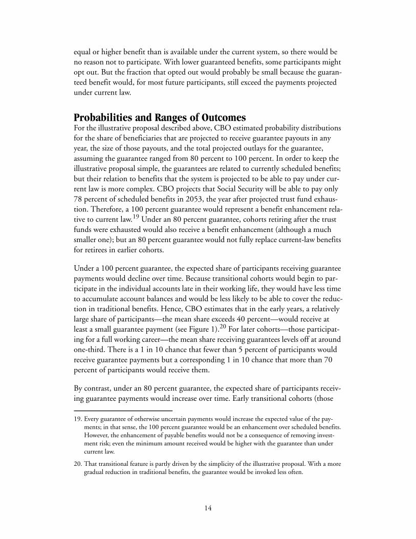
Under a 100 percent guarantee, the expected share of participants receiving guarantee payments would decline over time. Because transitional cohorts would begin to par-ticipate in the individual accounts late in their working life, they would have less time to accumulate account balances and would be less likely to be able to cover the reduc-tion in traditional benefits. Hence, CBO estimates that in the early years, a relatively large share of participants—the mean share exceeds 40 percent—would receive at least a small guarantee payment (see Figure 1).20 For later cohorts—those participat-ing for a full working career—the mean share receiving guarantees levels off at around one-third. There is a 1 in 10 chance that fewer than 5 percent of participants would receive guarantee payments but a corresponding 1 in 10 chance that more than 70 percent of participants would receive them.
By contrast, under an 80 percent guarantee, the expected share of participants receiv-ing guarantee payments would increase over time. Early transitional cohorts (those
19. Every guarantee of otherwise uncertain payments would increase the expected value of the pay-ments; in that sense, the 100 percent guarantee would be an enhancement over scheduled benefits. However, the enhancement of payable benefits would not be a consequence of removing invest-ment risk; even the minimum amount received would be higher with the guarantee than under current law.
20. That transitional feature is partly driven by the simplicity of the illustrative proposal. With a more gradual reduction in traditional benefits, the guarantee would be invoked less often.
14
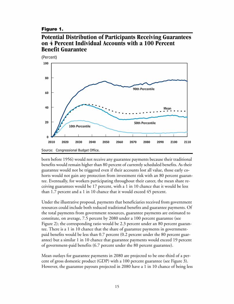
Figure 1.
Potential Distribution of Participants Receiving Guarantees on 4 Percent Individual Accounts with a 100 PercentBenefit Guarantee(Percent)
Source: Congressional Budget Office.
born before 1956) would not receive any guarantee payments because their traditional benefits would remain higher than 80 percent of currently scheduled benefits. As their guarantee would not be triggered even if their accounts lost all value, those early co-horts would not gain any protection from investment risk with an 80 percent guaran-tee. Eventually, for workers participating throughout their career, the mean share re-ceiving guarantees would be 17 percent, with a 1 in 10 chance that it would be less than 1.7 percent and a 1 in 10 chance that it would exceed 45 percent.
Under the illustrative proposal, payments that beneficiaries received from government resources could include both reduced traditional benefits and guarantee payments. Of the total payments from government resources, guarantee payments are estimated to constitute, on average, 7.5 percent by 2080 under a 100 percent guarantee (see Figure 2); the corresponding ratio would be 2.3 percent under an 80 percent guaran-tee. There is a 1 in 10 chance that the share of guarantee payments in government-paid benefits would be less than 0.7 percent (0.2 percent under the 80 percent guar-antee) but a similar 1 in 10 chance that guarantee payments would exceed 19 percent of government-paid benefits (6.7 percent under the 80 percent guarantee).
Mean outlays for guarantee payments in 2080 are projected to be one-third of a per-cent of gross domestic product (GDP) with a 100 percent guarantee (see Figure 3). However, the guarantee payouts projected in 2080 have a 1 in 10 chance of being less
2010 2020 2030 2040 2050 2060 2070 2080 2090 2100 2110
0
20
40
60
80
100
90th Percentile
50th Percentile10th Percentile
Mean
15

Figure 2.
Potential Distribution of Payouts from Benefit Guarantees as a Share of Total Social Security Benefits for 4 Percent Individual Accounts with a 100 Percent Benefit Guarantee(Percent)
Source: Congressional Budget Office.
than 0.02 percent and a 1 in 10 chance of exceeding 0.8 percent of GDP. With an 80 percent guarantee, mean outlays for guarantee payments are projected to be 0.1 percent of GDP in 2080, with the corresponding range of likely outcomes spanning 0.005 percent to 0.3 percent of GDP. To put those numbers in perspective, the imbal-ance between revenues and scheduled benefits in Social Security is expected to be just under 2.0 percent of GDP in 2080.
Market ValuesThe market value of the guarantee to beneficiaries today is calculated using options-pricing techniques. An 80 percent guarantee in the illustrative proposal with 4 percent individual accounts has a present market value of $0.4 trillion over a 75-year horizon (see Table 1). As the percentage of benefits that is guaranteed increases, the projected cost rises steeply. The guarantee cost, over the same horizon, reaches $0.9 trillion un-der a 90 percent guarantee and $1.9 trillion under a 100 percent guarantee.
To put those numbers in perspective, they could be compared to the present value of the imbalance between revenues and scheduled benefits in Social Security over the
2010 2020 2030 2040 2050 2060 2070 2080 2090 2100 2110
0
5
10
15
20
25
90th Percentile
50th Percentile
10th Percentile
Mean
16
Figure 3.
Potential Distribution of Total Guarantee Outlays for 4 Percent Individual Accounts with a 100 Percent Benefit Guarantee(Percentage of gross domestic product)
Source: Congressional Budget Office.
same period. CBO has estimated the present-value imbalance over the next 75 years to be about $1.9 trillion.21
The high sensitivity of the guarantee cost to the level of guaranteed benefits parallels the commonly observed high sensitivity of financial option prices to the strike price. A similar explanation, relating the guarantee to benefits under current law, can pro-vide some intuitive understanding of the sensitivity. As mentioned before, a 100 per-cent guarantee represents a benefit enhancement relative to current law. Its cost can thus be thought of as comprising two components, one being the cost of implicitly enhancing benefits and the other being the cost of assuming market risk. (For a paral-lel analysis using 2 percent individual accounts, see Appendix B.)
Comparison of the Alternative ApproachesThe difference in outcomes projected with and without consideration of the cost of market risk can be seen by comparing projected annual flows of the government’s
21. The fact that the estimates of the cost of providing a 100 percent guarantee and of Social Security’s fiscal imbalance are both $1.9 trillion is coincidental. The two estimates might not be equal with a different time horizon or with a differently designed proposal.
2010 2020 2030 2040 2050 2060 2070 2080 2090 2100 2110
0.0
0.2
0.4
0.6
0.8
1.0
90th Percentile
50th Percentile
10th Percentile
Mean
0
17

Table 1.
Changes in the Present Value of Payments over a 75-YearHorizon for Illustrative Proposals with 4 Percent Individual Accounts and Guarantees (Trillions of 2005 dollars)
Source: Congressional Budget Office.
a. The projected reduction in traditional benefits is measured against a baseline of scheduled ben-efits. However, the Social Security trust funds are not projected to be able to pay scheduled ben-efits throughout the 75-year horizon. Thus, the reduction would be smaller if measured relative to the current-law baseline.
b. Market values of guarantees are estimated using options-pricing techniques. After the trust funds were exhausted, beneficiaries in all cases would receive higher total benefits than are pro-jected under current law. With the 100 percent guarantee, all beneficiaries who were alive after the trust funds were exhausted would receive higher lifetime benefits than under current law, and no beneficiary would receive less.
guarantee cost with the expected guarantee payments calculated from the projected distributions of future outcomes. Under the illustrative proposal with a 100 percent guarantee, benefits paid out as guarantees are expected to total, on average, 0.3 per-cent of GDP in 2080. The equivalent annual cost, based on the options-pricing esti-mate, is three times that amount (see Figure 4). That difference arises from the fact that the distribution of future guarantee payments does not capture the value of the risk that is shifted from beneficiaries to the government (and thus to the taxpayers) when the government introduces a guarantee. The difference between the two lines represents the cost of that risk. In the market, certain future payments represented by the higher (solid) line would have the same price as the guarantee described in this paper, with mean payments represented by the lower (dashed) line.22
22. Several studies have suggested an alternative approach to assigning a flow of market-valued guaran-tee costs. In that approach, the distribution of future payouts is generated in a manner similar to the first method described in this paper, but with the expected rate of return on stocks set equal to the Treasury rate of return. That way, the estimated average annual government payouts under the guarantee reflect the market valuation of the risk. Theoretically, and in simulations, that approach leads to estimated guaranteed costs that match the estimates from the options-pricing model. See Pennacchi, “The Value of Guarantees on Pension Fund Returns,” and Lachance and Mitchell, “Guaranteeing Individual Accounts.”
-6.2 -6.2 -6.28.0 8.0 8.00.4 0.9 1.9___ ___ ___
Net difference 2.2 2.7 3.7
Difference from Scheduled-Benefits Baseline
Outlays to individual accountsMarket value of guaranteesb
Reduction in traditional benefitsa
Guaranteed Percentage of Scheduled Benefits80 90 100
18
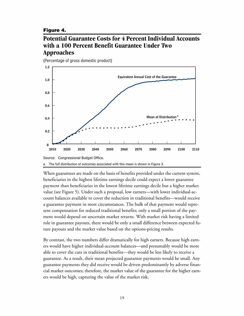
Figure 4.
Potential Guarantee Costs for 4 Percent Individual Accounts with a 100 Percent Benefit Guarantee Under Two Approaches(Percentage of gross domestic product)
Source: Congressional Budget Office.
a. The full distribution of outcomes associated with this mean is shown in Figure 3.
When guarantees are made on the basis of benefits provided under the current system, beneficiaries in the highest lifetime earnings decile could expect a lower guarantee payment than beneficiaries in the lowest lifetime earnings decile but a higher market value (see Figure 5). Under such a proposal, low earners—with lower individual-ac-count balances available to cover the reduction in traditional benefits—would receive a guarantee payment in most circumstances. The bulk of that payment would repre-sent compensation for reduced traditional benefits; only a small portion of the pay-ment would depend on uncertain market returns. With market risk having a limited role in guarantee payouts, there would be only a small difference between expected fu-ture payouts and the market value based on the options-pricing results.
By contrast, the two numbers differ dramatically for high earners. Because high earn-ers would have higher individual-account balances—and presumably would be more able to cover the cuts in traditional benefits—they would be less likely to receive a guarantee. As a result, their mean projected guarantee payments would be small. Any guarantee payments they did receive would be driven predominantly by adverse finan-cial market outcomes; therefore, the market value of the guarantee for the higher earn-ers would be high, capturing the value of the market risk.
2010 2020 2030 2040 2050 2060 2070 2080 2090 2100 2110
0.0
0.2
0.4
0.6
0.8
1.0
1.2
0
Mean of Distribution a
Equivalent Annual Cost of the Guarantee
19
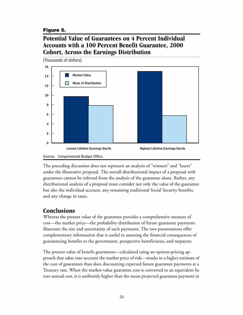
Figure 5.
Potential Value of Guarantees on 4 Percent Individual Accounts with a 100 Percent Benefit Guarantee, 2000 Cohort, Across the Earnings Distribution(Thousands of dollars)
Source: Congressional Budget Office.
The preceding discussion does not represent an analysis of “winners” and “losers” under the illustrative proposal. The overall distributional impact of a proposal with guarantees cannot be inferred from the analysis of the guarantee alone. Rather, any distributional analysis of a proposal must consider not only the value of the guarantee but also the individual account, any remaining traditional Social Security benefits, and any change in taxes.
ConclusionsWhereas the present value of the guarantee provides a comprehensive measure of cost—the market price—the probability distribution of future guarantee payments illustrates the size and uncertainty of such payments. The two presentations offer complementary information that is useful in assessing the financial consequences of guaranteeing benefits to the government, prospective beneficiaries, and taxpayers.
The present value of benefit guarantees—calculated using an options-pricing ap-proach that takes into account the market price of risk—results in a higher estimate of the cost of guarantees than does discounting expected future guarantee payments at a Treasury rate. When the market-value guarantee cost is converted to an equivalent fu-ture annual cost, it is uniformly higher than the mean projected guarantee payment in
Lowest Lifetime Earnings Decile Highest Lifetime Earnings Decile
0
2
4
6
8
10
12
14
16
Market Value
Mean of Distribution
20

the corresponding year, with the difference resulting from the inclusion of market risk in calculations based on market prices.
This paper illustrates two approaches that CBO would use to estimate the effects of guarantees under a simple hypothetical policy. It demonstrates the general order of magnitude of the benefits and costs associated with providing guarantees; however, it should not be assumed that the specific quantitative results can be applied to different plans. The value of guarantees is highly nonlinear, especially in the level of guaranteed benefits. Moreover, that value critically depends on the extent to which traditional Social Security benefits would be reduced under a given proposal with individual accounts. For that reason, these results cannot be extrapolated to plans with different guarantee percentages or different reductions in traditional benefits. Instead, each plan would need to be examined on its own using both of the methods described in this paper.
21


Appendix A:Options-Pricing Principles and the Discounting of Risky Cash Flows
Options pricing is based on the idea of dynamic hedging and the principle of no riskless arbitrage (usually shortened to “no arbitrage”). Dynamic hedging involves set-ting up a replicating portfolio (a portfolio that consists of securities of known values) so that its returns over a short period exactly match the option’s returns for any given scenario. As time passes, the replicating portfolio changes; dynamic hedging assumes rebalancing the portfolio continuously to match the instantaneous returns of the op-tion and its replicating portfolio. Under the principle of no arbitrage, two securities with identical returns must have identical prices; otherwise, by selling the more ex-pensive and buying the cheaper of the two, it would be possible to make profits with zero investment—an opportunity that cannot persist in an efficient market. There-fore, as long as it is possible to evaluate the price of the replicating portfolio, the price of the option can be uniquely determined.
The power of no-arbitrage pricing lies in its being independent of the purchaser’s (or seller’s) aversion to risk. As long as the securities included in the replicating portfolio are priced correctly, the option price will be unique and correct as well. In practice, that condition usually reduces to the requirement that the underlying security and a risk-free bond have well-defined market prices or, alternatively, known and well-de-fined fair values.
The widely used Black-Scholes formula derives from those principles and provides the price of a European option (one that can be exercised only at the specified expiration time), with a fixed strike price, on a stock that pays no dividends and whose price fol-lows a lognormal process (geometric Brownian motion). In practice, many options do not satisfy those restrictions, and numerical methods are used for pricing. The most popular classes of those methods are the binomial lattice and Monte Carlo methods.1
Binomial Lattice MethodsA lattice consists of a number of states (nodes), characterized by time and the price of the underlying security (stock, say). In each step (period) of the process, representing a short time interval, at any given node there are two possible outcomes—an “up” or “down” movement—with defined probabilities. A scenario of stock-price movements
1. For a more complete treatment of computational methods in pricing financial derivatives, see Robert L. McDonald, Derivatives Markets (Boston: Addison-Wesley, 2003).
23

is a path through the lattice. A binomial lattice has nodes chosen in such a way that the up movement from one node leads to the same next-period node as the down movement from the next-higher node. That structure limits the number of nodes—a useful feature for computational efficiency. As the number of steps increases (and the time intervals shorten), the lattice approximates the lognormal process implicit in the Black-Scholes formula. Indeed, for any option that can be priced by the formula, the two methods converge to the same result in the limit of infinitely many infinitesimally short steps.
Lattice methods are more flexible than analytic formulas. They are easily generalized to value options that can be exercised early (American options), options with multiple cash flows (either dividend payments or gradual investment over time), those with a stochastic (uncertain) strike price, and so on. For the purposes of this paper, periodic investments and stochastic strike price are particularly important.
Suppose there is a one-period put option on an underlying stock with a current (time 0) price, S, of $100 and two possible time 1 prices: $110 with a probability of 0.8 and $90 with a probability of 0.2. Let the strike price, K, be $98. What is the price of the put at time 0?
If the stock is worth $110 at time 1 (an up state), the put expires with no value. In the down state, the stock is worth $90 and the put is worth P = K – S = $8. To determine the price at time 0, the $8 figure must be multiplied by 0.2, the probability of the down state, as well as discounted to time 0. The result is 8 × 0.2 / (1 + r), where r is the appropriate rate of interest. The value of r is one of the most important questions in options-pricing theory.
Monte Carlo MethodsThe most obvious way to use a binomial lattice is to evaluate an option at its expira-tion date in all states and work backward through the lattice, computing the values at all nodes. That method works well if the lattice is fairly small (if it has relatively few periods). But for larger lattices, that method can result in prohibitively long computa-tion times (for instance, a lattice with 1,000 periods has 500,500 nodes). An alterna-tive method is to generate random outcomes (paths) of up-and-down movements and evaluate only the sample of nodes included in those paths. As in other applications, the methods that use randomly generated paths and average the results over those paths are called Monte Carlo methods.
Additionally, Monte Carlo methods can avoid using a lattice altogether and generate random sizes of up-and-down steps from a continuous distribution.
As opposed to straightforward lattice methods, Monte Carlo methods compute values along a path going forward, rather than backward. Backward computation is pre-
24

cluded by the fact that not all future states have been computed by the time a given node is evaluated.
Proper Discounting and Risk-Neutral ValuationA naïve approach to discounting might follow the logic of simple capital budgeting: uncertain cash flows can be represented by their expected value but discounted at a higher rate, which reflects the fact that they are less desirable to risk-averse investors than are certain cash flows with the same expected value. Although that reasoning is correct for comparing a firm’s investment opportunities, it fails in options valuation in a financial market because it creates opportunities for riskless arbitrage.
One might be tempted, perhaps, to use the expected return on the stock (6 percent in the above example) as the discount rate. The expected return is, after all, the rate that properly prices the underlying stock. This approach would result in the put price of 8 × 0.2/1.06 = 1.51. Is that price sustainable in an efficient market?
Consider a risk-free security—such as a short-term, zero-coupon, government bond—with a period rate of return of 2 percent. If one unit of the bond pays $100 at maturity (time 1), its price at time 0 is 100/1.02 = 98.04. Now consider an investor who, at time 0, buys 0.44 units of this bond and sells short 0.4 shares of stock. At time 1, the investor has $44 in bonds and owes, for the short sale of stock, either $44 (in the up state) or $36 (in the down state). The total value of the portfolio at time 1 is $8 in the down state and zero in the up state—exactly the same as the put option. This is the replicating portfolio alluded to earlier. It is important to note that the port-folio and the put option have identical values on a state-by-state basis, not merely equal probability distributions of values. The option’s cash flows are indistinguishable from those of its replicating portfolio; hence, their prices must be equal.
However, the price of the replicating portfolio is known to be 44/1.02 – 40 = 3.14, which is the price of the put. That price is more than double the price calculated earlier.
Why was the first calculation wrong? Using the 6 percent rate for discounting is not justifiable. The put does not have the same risk characteristics as the underlying stock. It differs from the stock in three important ways, all of which affect its value:
B The volatility of option returns is much greater than the volatility of stock returns. In this example, the stock price changes by 10 percent up or down from time 0 to time 1; the put value changes by 100 percent down and by even more up (155 per-cent when computed correctly, 430 percent in the naïve attempt).
B The volatility of the option changes as the value of the underlying stock changes relative to the strike price. That will become more apparent in the next example, but it is obvious that this option would have had a certain value of zero if the strike
25
price had been below $90 and a value mirroring the stock price (with a constant offset) if the strike price had been above $110.
B The put price is dependent on the underlying price, and the two securities together can form a perfect hedge for stock-price movements below the strike price. Conse-quently, as an addition to a portfolio, the put actually reduces risk.
By itself, the first point would suggest the need for using a higher discount rate. The last property would suggest the need for a lower rate. The second one makes the dis-count rate (in the more general case with more than one period) path-dependent and, hence, usually intractable. Together, those considerations help explain why the naïve approach is wrong, but they do not help determine the proper rate.
The solution is based on a simple but powerful insight: if the option and its replicat-ing portfolio have identical cash flows, any investor would find their values equal. Here, “any investor” can mean, among other things, having any level of risk aversion. But if that is true for any level of risk aversion, it is true for zero risk aversion as well. Thus, the use of a replicating portfolio allows the option to be priced from the per-spective of a risk-neutral investor. Moreover, price identity based on replication would hold even if all market participants were risk-neutral. Thus, the computation of the option price can proceed as if the market were operating in a risk-neutral world.
In a risk-neutral world, however, investors would not demand compensation for risk, so risky securities would not yield a higher rate of return. In other words, every secu-rity would have the same rate of return, the risk-free rate.2 That property avoids the problem arising from the second point above: option returns that change over time and across paths.
This insight implies that options pricing should start with a preparatory step: adjust-ing the rates of return on any risky securities involved. The binomial lattice (or Monte Carlo steps) must be consistent with risk-neutral valuation, so the expected rate of re-turn on the underlying stock must equal the risk-free rate. At the same time, the vola-tility of its returns must be preserved because that volatility is a key determinant of the option price. If the up and down steps were of equal sizes in the first place, it would suffice to change the associated probabilities. Only after that step can the evaluation on the lattice be done as described earlier, and the final values can then be discounted using the risk-free rate.
In this example, the stock’s expected return in the risk-free world would have to be 2 percent. That behavior can be achieved by changing the up probability to 0.6 (and consequently, the down probability to 0.4). As a result, the put would be worth $8 at time 1 with probability 0.4, which then must be discounted to time 0 using the risk-
2. Note that the actual risk aversion is still reflected in the prices of ordinary (as opposed to derivative) assets, such as stocks, and that this analysis takes those prices as given.
26
free rate of 2 percent. Consequently, the price is 8 × 0.4/1.02 = 3.14, as already com-puted using a replicating portfolio.3
An Example of Pricing a Put OptionThe previous section showed how to construct a basic building block of options pric-ing, but it involved too few states to demonstrate the dynamic aspect of replicating portfolios and the path-dependent volatility of options. This section extends the lat-tice by another period (see Figure A-1). The put option is on the same stock, the strike price remains $98, but the expiration time is now 2. The option is European, meaning that it cannot be exercised before expiration.
For times 0 and 1, the lattice looks just as it did in the previous example (the risk-neu-tral version, of course). In the next period, the stock can go up or down from each of the two time 1 nodes. Assuming constant volatility, all movements will again be ±10 percent. Thus, from the up node ($110), the stock can go up again, to $121, or down, to $99. From the down node ($90), it can go up to $99 or down to $81. Note that up-down and down-up paths result in the same value, which can be represented as a single node. (That is the recombination property of binomial lattices.)
Pricing is straightforward. The only final state with a positive put value is the down-down state, wherein the put is worth $98 – $81 = $17. The (risk-neutral) probability of that outcome is 0.42 = 0.16, and the price, discounted to time 0, is thus 17 × 0.16 / 1.022 = 2.61438.
It is instructive to see what happens to the put as the uncertainty is gradually resolved. If the first movement is up, the put price at time 1 will be exactly zero, as it will expire without value in either of the final states reachable from the up node. If the first movement is down, the put price at time 1 will be 17 × 0.4/1.02 = 6.66667. That is the price for which the holder of the put could sell in an efficient market. If the holder could exercise the option then, he or she would prefer to do so, as it would be worth $8, but early exercise is not allowed for this option. (If early exercise were allowed, it would increase the value of the put at time 1, which in turn would increase its value at time 0.) The replicating portfolio at this node would involve selling short 17/18ths of
3. The continuous-time version of the described risk-neutral approach is built into the Black-Scholes formula. That is why input parameters in Black-Scholes include the risk-free rate and the volatility of stock, but not the expected rate of return on stock. The option price can also be computed on a lattice using real-world returns and probabilities instead of resorting to the risk-neutral-world con-cept. However, using that approach requires knowing the option prices in all future states attain-able from the node being computed. That, in turn, requires backward computation on a lattice and precludes the use of computationally more efficient Monte Carlo methods. The final result for the option price is the same with the risk-neutral measure as it is with the real-world measure because the methods are mathematically equivalent; therefore, the computationally more efficient method is preferable.
27
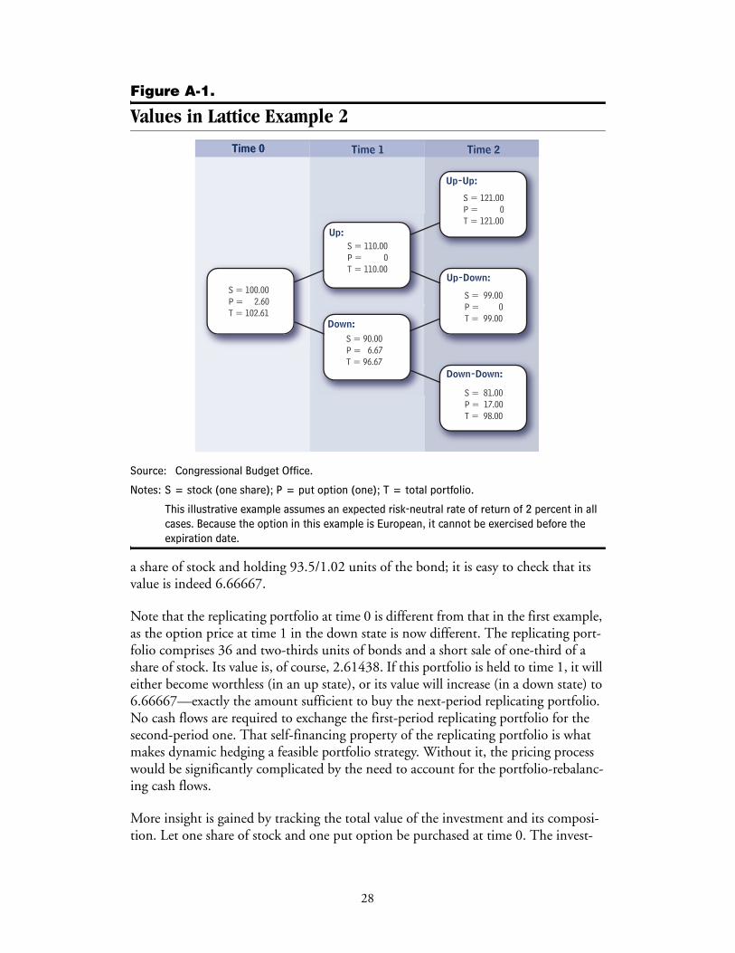
Figure A-1.
Values in Lattice Example 2
Source: Congressional Budget Office.
Notes: S = stock (one share); P = put option (one); T = total portfolio.
This illustrative example assumes an expected risk-neutral rate of return of 2 percent in all cases. Because the option in this example is European, it cannot be exercised before the expiration date.
a share of stock and holding 93.5/1.02 units of the bond; it is easy to check that its value is indeed 6.66667.
Note that the replicating portfolio at time 0 is different from that in the first example, as the option price at time 1 in the down state is now different. The replicating port-folio comprises 36 and two-thirds units of bonds and a short sale of one-third of a share of stock. Its value is, of course, 2.61438. If this portfolio is held to time 1, it will either become worthless (in an up state), or its value will increase (in a down state) to 6.66667—exactly the amount sufficient to buy the next-period replicating portfolio. No cash flows are required to exchange the first-period replicating portfolio for the second-period one. That self-financing property of the replicating portfolio is what makes dynamic hedging a feasible portfolio strategy. Without it, the pricing process would be significantly complicated by the need to account for the portfolio-rebalanc-ing cash flows.
More insight is gained by tracking the total value of the investment and its composi-tion. Let one share of stock and one put option be purchased at time 0. The invest-
Time 0Time 0 Time 1 Time 2
S = 100.00P = 2.60T = 102.61
S = 110.00P = 0T = 110.00
Up:
Down:S = 90.00P = 6.67T = 96.67
Up-Up:
S = 121.00P = 0T = 121.00
Up-Down:
S = 99.00P = 0T = 99.00
Down-Down:
S = 81.00P = 17.00T = 98.00
28

ment will follow one of 4 paths given by the nodes in Figure A-1. On an expected-value basis, the put loses value as time passes. That outcome is to be expected, aspart of an option’s value derives from uncertainty captured by time to expiration. However, the stock return more than makes up for the put option’s loss, and the total portfolio is always expected to earn more than the risk-free rate, as long as its return is uncertain.
Moreover, the expected rate of return on the total portfolio increases with uncertainty, just as one would expect. However, the uncertainty of that return varies widely: its standard deviation is 5.2 percent at time 0, 8 percent at time 1 in the up state, and 0.41 percent in the down state. Indeed, the risk premium (over the risk-free rate) is proportional to the standard deviation, indicating that the price of risk is constant. No such consistency would have been obtained by a naïve approach such as that described in conjunction with the first example.
29


Appendix B:Estimations of Guarantee Costs with
2 Percent Accounts
To test the sensitivity of the options-pricing projections to a simple change of scale, the Congressional Budget Office also examined a hypothetical proposal in which 2 percent rather than 4 percent of taxable earnings was redirected from the Social Security Trust Funds to individual accounts. In that case, the traditional portion of the Social Security benefit would be reduced to about 72 percent of scheduled bene-fits in the long run. Thus, the reduction, relative to currently scheduled benefits, would be exactly half the reduction in the 4 percent plan. The reduction would also be halved for transitional cohorts, so that traditional benefits would be reduced by 5 percent for the 1950 cohort.
With a 100 percent guarantee, the cost of the guarantee would be half as much in the 2 percent plan as in the 4 percent plan. In that special case, the cost is proportional to the size of the redirection (see Table B-1). However, two special conditions present in that example are necessary to maintain that proportionality. First, the 100 percent guarantee level is critical; second, in the design of the illustrative proposal, tax redirec-tions and benefit cuts are tied together and scaled proportionally. If either of those two conditions is relaxed, the proportionality of costs to the size of tax redirection no longer holds. When guaranteed income levels are lowered, the cost falls more rapidly in the plan with the smaller individual account redirection because the cut in tradi-tional benefits is smaller. Thus, by definition, the possible gap between those benefits and any guarantee is smaller.
31

Table B-1.
Changes in the Present Value of Payments over a 75-YearHorizon for Illustrative Proposals with 2 Percent Individual Accounts and Guarantees(Trillions of 2005 dollars)
Source: Congressional Budget Office.
Note: * = absolute value of less than $50 billion.
a. The projected reduction in traditional benefits is measured against a baseline of scheduled ben-efits. However, the Social Security trust funds are not projected to be able to pay scheduled ben-efits throughout the 75-year horizon. Thus, the reduction would be smaller if measured relative to the current-law baseline.
b. Market values of guarantees are estimated using options-pricing techniques. After the trust funds were exhausted, beneficiaries in all cases would receive higher total benefits than are pro-jected under current law. With the 100 percent guarantee, all beneficiaries who were alive after the trust funds were exhausted would receive higher lifetime benefits than under current law, and no beneficiary would receive less.
-3.1 -3.1 -3.14.0 4.0 4.0
* 0.2 0.9___ ___ ___Net difference 0.9 1.1 1.8
80 90 100Guaranteed Percentage of Scheduled Benefits
Reduction in traditional benefitsa
Outlays to individual accountsMarket value of guaranteesb
Difference from Scheduled-Benefits Baseline
32