Evaluating Density Forecasts: Is Sharpness Needed?

James Mitchell1 and Kenneth F. Wallis2

1National Institute of Economic and Social Research

[J.Mitchell@niesr.ac.uk]

2University of Warwick [K.F.Wallis@warwick.ac.uk]

First version, 26 August 2008 Summary. In a recent article Gneiting, Balabdaoui and Raftery (Journal of the Royal Statistical Society B, 2007) propose the criterion of sharpness for the evaluation of predictive distributions or density forecasts. They motivate their proposal by an example in which standard evaluation procedures based on probability integral transforms cannot distinguish between the ideal forecast and several competing forecasts. In this paper we show that their example has some unrealistic features which make it an insecure foundation for their argument that existing calibration procedures are inadequate in practice. We present an alternative, more realistic example in which relevant statistical methods provide the required discrimination between competing forecasts, and argue that there is no need for a subsidiary criterion of sharpness. Keywords: Calibration; Density forecast; Predictive distribution; Probability integral transform; Tests of autocorrelation; Tests of fit JEL Classification numbers: C22, C53 Acknowledgments Some preliminary results were presented at the Oxford Forecasting and Decision Analysis Group, March 2008. We are grateful to seminar participants and Tilmann Gneiting for helpful comments. James Mitchell also acknowledges support by the ESRC under award RES-000-22-1390.

1. Introduction

Forecasts for an uncertain future are increasingly presented probabilistically. Tay and Wallis

(2000) survey applications in macroeconomics and finance, and in a recent editorial Gneiting

(2008) urges further efforts. When the focus of attention is the future value of a continuous

random variable, the presentation of a density forecast or predictive distribution – an estimate

of the probability distribution of the possible future values of the variable – represents a

complete description of forecast uncertainty. It is then important to be able to assess the

reliability of forecasters’ statements about this uncertainty. Dawid’s prequential principle is

that assessments should be based on the forecast-observation pairs only; this ‘has an obvious

analogy with the Likelihood Principle, in asserting the irrelevance of hypothetical forecasts

that might have been issued in circumstances that did not, in fact, come about’ (Dawid, 1984,

p.281). A standard approach is to calculate the probability integral transform values of the

outcomes in the forecast distributions, and assessment rests on ‘the question of whether

[such] a sequence “looks like” a random sample from U[0,1]’ (p.281; quotation marks in the

original). If so, the forecasts are said to be well-calibrated.

In a recent article, Gneiting, Balabdaoui and Raftery (2007) propose the paradigm of

maximising the sharpness of the predictive distributions subject to calibration for the

evaluation of forecasts. Sharpness refers to the concentration of the predictive distributions

and is a property of the forecasts only, although the condition of calibration remains a

property of the forecast-observation pairs. They motivate their argument by an example in

which four different forecasts are shown, in a simulation experiment, to produce uniform

probability integral transforms, hence this requirement cannot distinguish between them.

Since one of them is the ‘ideal’ or correct forecast, ‘this is a disconcerting result’ (2007,

p.245), which leads to the authors’ argument that there is a need for additional criteria.

However their example has two unrealistic features, from the point of view of practical

forecast evaluation, which make it an insecure foundation on which to base their claim that

existing evaluation methods are inadequate. One concerns their approach to forecast

combination, while the second is the absence of a time dimension. Our first purpose in this

paper is to elaborate these shortcomings. We then show that, in more realistic settings, the

‘disconcerting result’ no longer applies and the calibration requirement as posed by Dawid

can indeed distinguish the ‘ideal’ forecast from its competitors. Hence we question the

perceived need for the sharpness criterion.

1

The rest of the paper proceeds as follows. Section 2 briefly describes the statistical

framework for the problem at hand. Section 3 presents the example of Gneiting, Balabdaoui

and Raftery (2007), hereafter GBR, and disputes the conclusions they draw from it. Section 4

presents a second example, and shows how existing statistical methods facilitate density

forecast evaluation and comparison. Section 5 concludes.

2. The statistical framework

We consider probabilistic forecasts in the form of predictive cumulative distribution

functions (CDFs) . These may be based on statistical models, supplemented by

expert judgment. The outcome is a random variable with distribution , which

represents the true data-generating process. If

, 1, 2,...tF t =

tX tG

tF Gt= for all t, GBR speak of the ‘ideal’

forecaster; in economic forecasting this is commonly referred to as a ‘rational’ or ‘full-

information’ forecast.

In making forecasts for the future, Dawid’s prequential forecaster, at any time t, with

the values of the sequence ( )tx ( )( )1 2, ,...,t

tX X X=X to hand, issues a forecast distribution

for the next observation 1tF + 1tX + . As noted above, the standard tool for assessing forecast

performance on the basis of the forecast-observation pairs is the sequence of probability

integral transform (PIT) values

( )t t tp F x= .

If coincides with , , then the tF tG 1, 2,...t = stp are independent uniform U[0,1] variables.

An advantage of basing forecast evaluation on the PIT values is that it is not necessary to

specify , real or hypothesised. Uniformity is often assessed in an exploratory manner, by

inspection of histograms of PIT values, for example, while formal tests of goodness-of-fit are

also available, as are tests of independence. Smith (1985) describes diagnostic checks that

can be applied to a range of time-series models, while Diebold, Gunther and Tay (1998)

introduce these procedures to the econometrics literature and provide a full proof of the

iidU[0,1] result.

tG

2

GBR define probabilistic calibration of the sequence relative to the sequence

as the condition

tF tG

( )1

1

1 ( ) for all (0,1)T

t tt

G F p p pT

−

=→ ∈∑ . (1)

Their theorem 2 (2007, p.252) shows that probabilistic calibration is equivalent to the

uniformity of the PIT values. Intuitively, and dropping time subscripts for convenience,

given a CDF and the transformation ( )G x ( )p F x= , the standard change-of-variable

approach gives the CDF ( )H p , say, as the expression inside the summation in equation (1):

if ( )H p = p then p has a uniform distribution. Condition (1) is a convenient device for

checking probabilistic calibration in circumstances where is known, as in simulation

experiments or theoretical exercises which require the data-generating process to be

specified. We note, however, that neither this definition nor any other discussion of the

theoretical framework in Section 2 of GBR’s article makes any reference to the independence

component of the proposition discussed in the preceding paragraph, although occasional

references appear elsewhere in the article.

tG

3. GBR’s example

The scenario for the simulation study is that, each period, nature draws a standard normal

random number tµ and specifies the data-generating distribution . Four

competing forecasts are constructed. The ideal forecaster conditions on the current state and

issues the forecast

( ,1t tG N µ= )

ttF G= . The ‘climatological’ forecaster, having historical experience in

mind, takes the unconditional distribution (0,2)tF N= as their probabilistic forecast. The

remaining two forecasts are combined forecasts, motivated by an example of Hamill (2001).

Hamill’s forecaster is a master forecaster who assigns the forecasting problem with equal

probability to any of three student forecasters, each of whom is forecasting incorrectly: one

has a negative bias, one has a positive bias, and the third has excessive variability. Thus the

forecast distribution is ( )2,t t tN µ δ σ+ , where ( )2, (0.5,1), ( 0.5,1) or (0,1.69)t tδ σ = − , each

with probability one-third. Similarly GBR’s ‘unfocused’ forecaster observes the current state

but adds a distributional bias as a mixture component, giving the forecast distribution

3

( ) ( ){ }0.5 ,1 ,1t t tN Nµ µ τ+ + where 1tτ = ± , each with probability one-half. With 10,000

random draws of tx from , GBR obtain the PIT histograms for the four forecasters shown

in Fig. 1 (reproduced from the original).

tG

The four PIT histograms are ‘essentially uniform’, which ‘is a disconcerting result’ (2007, p.

245), because these PIT histograms cannot distinguish the ideal from the competing forecasts.

However panels (c) and (d) of Fig. 1 are the result of an unusual approach to forecast

combination. In panel (c), for example, the unfocused forecaster is treated as two separate

forecasters, whose PIT histograms are combined to give the result shown. The forecast

issued is either ( ) ( ){ }0.5 ,1 1,1t tN Nµ µ+ + or ( ) ( ){ }0.5 ,1 1,1t tN Nµ µ+ − , and GBR

calculate the PIT of a given outcome in the relevant distribution. Thus an observer is

assumed to know which of the two forecasts was issued at a given point in time, and is

thereby able to split the sample into two independent sub-samples and calculate two separate

PIT histograms, one for each component forecaster. Similarly, what is shown in panel (d) of

Fig. 1 is the average of three separate PIT histograms, one for each of the three student

forecasters: again an observer is implicitly assumed to know which student issued a given

forecast, and the three student forecasters are being separately evaluated. We reproduce

GBR’s experiment to obtain the corresponding PIT histograms of the component forecasters.

Fig. 2 shows the two resulting PIT histograms that are combined to produce panel (c) of their

4

Fig.1, shown above, and the three histograms that produce panel (d). Each panel of Fig. 2

shows departures from uniformity, as expected, and an observer would conclude that none of

the forecasts is satisfactory. It is not clear what practical interest then resides in combining

the component histograms.

Fig. 2. Component PIT histograms for the unfocused forecaster [panel (c) of Fig.1] and Hamill’s forecaster [panel (d) of Fig.1]

On the other hand the presentation of the problem by GBR indicates that it is the

performance of a single forecaster that is the focus of attention in each case – Hamill’s master

forecaster or their unfocused forecaster. If the forecasts in the former case are to be treated as

5

a single series by an observer who regards this as the master forecaster’s output, without

being able to identify which student produced which forecast, then the appropriate combined

forecast to study is given as the superposition of the component conditional forecasts, in other

words as a finite mixture distribution, in the sense of Everitt and Hand (1981), for example.

And likewise for the unfocused forecaster. Accordingly we replicate the simulation

experiment with the appropriate finite mixture distribution representing these two forecasters,

namely:

unfocused: ( ) ( ){ } ( ) ( ){ }0.25 ,1 1,1 0.25 ,1 1,1t t t t tF N N N Nµ µ µ µ= + − + + + (2)

Hamill: ( ) ( ) (0.33 0.5,1 0.33 0.5,1 0.33 ,1.69t t t tF N N Nµ µ= + + − + )µ . (3)

This produces the less disconcerting results shown in Fig. 3: these PIT histograms can indeed

distinguish forecasts (c) and (d) from the ideal forecast. Their forecast variances are too

large, so that the tails of the forecast densities contain too few of the observations and the PIT

histograms are correspondingly hump-shaped.

Fig. 3. Our PIT histograms for (a) the ideal forecaster, (b) the climatological forecaster, (c) the unfocused forecaster and (d) Hamill’s forecaster

6

The condition in equation (1) also allows us to verify that, with this interpretation,

neither the unfocused forecaster nor Hamill’s forecaster is probabilistically calibrated,

contrary to GBR’s claims. For the unfocused forecast mixture distribution (2) we follow

their approach and equate the limit in (1) to the typical term evaluated at 0tµ = . Consider

the pth quantile, , namely the value x such that 1( )F p−

0.5 ( ) 0.25 ( 1) 0.25 ( 1)x x xΦ + Φ − + Φ + = p ,

where Φ is the standard normal CDF. For such a value, is it the case that ?

For we have in both distributions by symmetry of the normal distribution. But

in all other cases the condition fails. Take

( ) ( )G x x p= Φ =

0.5p = 0x =

1x = , for example. Then

( ) 0.5 0.8413 0.25 0.5 0.25 0.9772 0.79F x = × + × + × = .

That is, . But , contrary to their claim of probabilistic

calibration. Similarly representing Hamill’s forecaster as the mixture distribution (3), the pth

quantile satisfies

1(0.79) 1F− = (1) 0.8413 0.79G = ≠

1 1 1( )3 2 2 1.3

xF x x x p⎧ ⎫⎛ ⎞ ⎛ ⎞ ⎛ ⎞= Φ − +Φ + +Φ =⎨ ⎬⎜ ⎟ ⎜ ⎟ ⎜ ⎟⎝ ⎠ ⎝ ⎠ ⎝ ⎠⎩ ⎭

.

With we obtain , whereas 1.3x = ( ) 0.8645F x = (1.3) (1.3) 0.9032G = Φ = . The deviation of

0.0387 exceeds the maximum claimed deviation of 0.0032, calculated by GBR to support

their statement that “the probabilistic calibration condition is violated, but only slightly so,

resulting in deceptively uniform PIT histograms”. Their calculations are based on averaging

(mixing) the pth quantiles of the component distributions. Again this is an unusual approach

to forecast combination, and it does not in general give the pth quantile of the mixture

distribution.

The climatological or unconditional forecaster is then the remaining forecaster who

cannot be distinguished from the ideal forecaster by their PIT histograms. However the GBR

example is concerned with forecasting white noise, whereas time dependence that gives

simple criteria for distinguishing between conditional and unconditional forecasts is a feature

of more typical forecasting problems. Their example has the same structure as an example

given by Granger (1983), in a paper entitled “Forecasting white noise”. However Granger’s

formulation takes an explicit time-series forecasting perspective: “if 1t t tx y − e= + where

are independent, pure white noise series, then if is observable, , t ty e ty tx will be pure

7

white noise but forecastable ... Thus, tx is not forecastable just from its own past but

becomes forecastable when past values of are added to the information set” (1983, p.308).

From a practical forecasting perspective, in discrete time, the assumption in GBR’s example

that the state variable

ty

tµ is observable could be made explicit via a similar timing

convention. Equally, however, forecasting a white noise process is scarcely a representative

example in time-series forecasting, and to better motivate a fuller discussion of relevant

criteria we introduce time dependence via a simple autoregressive process.

4. Forecasting an autoregressive process

Consider the Gaussian AR(2) data generating process

( )21 1 2 2 , ~ 0,t t t t tY Y Y N εφ φ ε ε σ− −= + + .

The true or ‘ideal’ forecast distribution of given observations tY 1ty − and and

knowledge of parameter values is

2ty −

( )21 1 2 2,t t tG N y y εφ φ σ− −= + .

The ‘climatological’ or unconditional probability forecast is

( )20,U t yF N σ=

where ( )2 21 1 2 21 yεσ φ ρ φ ρ σ= − − , 1, 2i i and ρ = , are autocorrelation coefficients:

( )1 1 21ρ φ φ= − and 2 1 1 2ρ φ ρ φ= + .

We consider a variant forecaster who assumes that the data are generated by a first-

order autoregression and issues the forecast

( )21 1 1,t tF N y 1ρ σ−=

while, with the same assumption, a second variant is subject to a one-period data delay, so the

forecast is

( )22 2 2,t tF N y 2ρ σ−= ,

8

where ( )2 21 11 y

2σ ρ σ= − and ( )222

21 yσ 2ρ σ−= . We assume that these forecasters use least-

squares regression of y on lagged y to estimate the relevant coefficient and associated residual

variance, but as above we neglect parameter estimation error and use the corresponding ‘true’

values.

Finally, an ‘average’ forecaster knows that combining can often be of benefit and so

constructs the equally-weighted combined forecast

( ) ( )2 21 1 1 2 2 20.5 , 0.5 ,Ct t tF N y N yρ σ ρ− −= + σ ,

which is an example of a finite mixture distribution, as above. The composite information set

for the combined density forecast is identical to the information set of the true forecast

density: both contain the same two observations. However the combined forecast uses the

information inefficiently, relative to the true forecast. It yields, despite the fact that we know

the true distribution is Gaussian, a mixture normal density forecast.

We assess the performance of these five forecasts in a further simulation study, using

a variety of evaluation criteria discussed in turn below. To assess the effect of time

dependence on the performance of these criteria we consider four pairs of values of the

autoregressive parameters 1φ and 2φ , as shown in Table 1. Each delivers a stationary AR(2)

process, with differing degrees of autocorrelation, also as shown in Table 1. Case (2) exhibits

rather less persistence than is observed in the variables for which central banks often publish

density forecasts, namely inflation and GDP growth. The structure of case (3) is such that the

AR(1) forecast coincides with the unconditional forecast , while the AR(lag) forecast

coincides with the ideal forecast , thus the combined forecast is a combination of

the correct conditional and unconditional forecasts in this case. We report results based on

500 replications and a sample size

1tF UtF

2tF tG CtF

150T = , which is typical of applications in

macroeconomics.

4.1. PIT histograms

We first present histograms of PIT values, to allow an informal assessment of their

uniformity and hence of probabilistic calibration in GBR’s sense. We note that the assumed

distributions of the density forecasts, in respect of their normality and their first two moments

9

conditional on the information on which they are based, are correct for all but the

combination forecast. The results presented in Fig. 4 are then completely as expected.

The PIT histograms in the first four columns of Fig. 4 are ‘essentially uniform’ and

cannot distinguish the ideal forecast from its first three competitors. Its fourth competitor, the

combination forecast, has too great a variance in all cases, hence all four PIT histograms in

the last column of Fig. 4 have a humped shape. This is most striking in case (3) where, of the

two components in the combination, the AR(1) forecast, here the unconditional forecast, has

an error variance which exceeds that of the AR(lag) or ideal forecast by a factor of ten.

Fig. 4. PIT histograms in Cases 1-4 for (a*) the ideal forecaster, (b*) the climatological forecaster, (c*) the AR(1) forecaster, (d*) the ARlag forecaster and (e*) the combination

forecaster

4.2. Goodness-of-fit tests

Formal tests of goodness-of-fit can be based on the PIT values tp or on the values given by

their inverse normal transformation, ( )1tz −= Φ tp , where ( )Φ ⋅ is the standard normal

distribution function (Smith, 1985; Berkowitz, 2001). If tp is iidU(0,1), then is iidN(0,1). tz

10

The advantages of this second transformation are that there are more tests available for

normality, it is easier to test autocorrelation under normality than uniformity, and the normal

likelihood can be used to construct likelihood ratio tests. In the present exercise four of the

density forecasts are explicitly based on the normal distribution; here the double

transformation returns as the standardised value of the outcome , which could be

calculated directly.

tz ty

We consider the classical Kolmogorov-Smirnov (KS) and Anderson-Darling (AD)

tests for uniformity, together with the Doornik-Hansen (DH) test for normality (Doornik and

Hansen, 1994). These are all based on random sampling assumptions, and there are no

general results about their performance under autocorrelation. Table 2 reports the rejection

percentages for each of these goodness-of-fit tests at the nominal 5% level for each of the five

density forecasts. For the KS and AD tests we use simulated critical values for the sample

size of 150, while the DH test statistic is approximately distributed as chi-square with two

degrees of freedom under the null.

The results show that the goodness-of-fit tests tend not to reject any of the conditional

forecasts. The rejection rates for the ideal forecasts, which have white noise errors, are not

significantly different from the nominal 5% level. Autocorrelation clearly affects the

performance of the tests for the two variant forecasts and their combination, but, in general,

the rejection rate is not greatly increased. The unconditional or ‘climatological’ forecasts

have the greatest error autocorrelation, and this is associated with a substantial increase in the

rejection rates of the goodness-of-fit tests. In case (3) the AR(1) forecast and the

unconditional forecast coincide, and the high rejection rate in this case also spills over to the

combined forecast. In other cases these tests suggest that the combined forecast’s normal

mixture distribution appears not to deviate too much from normality. The results in the last

row suggest that the AD test has greater power than the KS test, which is consistent with

results obtained by Noceti, Smith and Hodges (2003) in the white noise case.

4.3. Autocorrelation tests

Test of independence can be based on the tp or series, as noted above. For the PIT series

we consider the Ljung-Box (LB) test, based on autocorrelation coefficients up to lag four,

approximately distributed as chi-square with four degrees of freedom under the null. For

tz

11

their inverse normal transforms we consider a widely used parametric test due to Berkowitz

(2001) which, under a maintained hypothesis of normality, tests jointly for correct mean and

variance (‘goodness-of-fit’), and independence. It is a likelihood ratio test, denoted Bk

below, approximately distributed as chi-square with three degrees of freedom. For the

independence component of the joint null hypothesis the alternative is that follows an

AR(1) process. In the present exercise the mean and variance of differ from (0,1) only in

the case of the combination forecast, thus for the first four forecasts the test is, in effect, a test

of the first-order autocorrelation coefficient of the point forecast errors.

tz

tz

The results in Table 3 show that adding a test of independence to the evaluation tool-

kit immediately enables us to distinguish the ideal forecast from the competing forecasts.

The rejection rates for the ideal forecasts are close to the nominal size of the (asymptotic)

tests. For the other forecasts the tests have good power: in case (1), a relatively persistent

series, there are no Type 2 errors in our 500 replications for any of the competing forecasts.

This is also true of the unconditional forecasts in cases (3) and (4). Whereas Figure 4 might

be thought to represent a ‘disconcerting result’ since it does not distinguish the ideal forecast

from three of its competitors, we see that considering both components of the calibration

requirement, namely independence and uniformity of the PITs, delivers the desired

discrimination between forecasts.

4.4. Scoring rules and distance measures

Scoring rules evaluate the quality of density forecasts by assigning a numerical score based

on the forecast and the subsequent realisation of the variable. A popular choice, originally

proposed by Good (1952), is the logarithmic score

( ) (log log )j t jtS y f y= t

for forecast density jtf . To a Bayesian the score is the predictive likelihood, and if two

forecasts are being compared, the log Bayes factor is the difference in their logarithmic

scores. If one of the forecasts is the true density , then the expected difference in their

logarithmic scores is the Kullback-Leibler information criterion (KLIC) or distance measure

tg

{ }KLIC log ( ) log ( )t t t jtE g y f y= − t

where the expectation is taken in the true distribution. In a similar manner to the use of the

mean error or bias in a point forecast, the KLIC can be interpreted as a density forecast error.

12

Replacing E by a sample average, and using transformed variables , a KLIC-based test is

used for density forecast evaluation by Bao, Lee and Saltoglu (2004, 2007) and Mitchell and

Hall (2005).

tz

In the present exercise, with density forecasts based on normal distributions, the

expected logarithmic score is a simple function of the forecast variance (‘sharpness’), namely

{ } ( )21 12 2log ( ) log 2j jE f y πσ= − − .

For the combination forecast, with a normal mixture distribution, we calculate the

corresponding expectation by numerical integration. Table 4 then reports the KLIC value

together with the average logarithmic score for each forecast (both multiplied by 100); with

the present sample size and number of replications the simulation-based average score

scarcely deviates from the expected score calculated analytically.

Since the KLIC of a given forecast is the difference between its logarithmic score and

that of the ideal forecast, the two criteria in Table 4 rank the forecasts identically. The

differences reflect the value of the information used by each forecast in each case. The

unconditional or climatological forecast uses no information from past data and is ranked last,

but this is least costly in case (2), where the data are least persistent. The AR(1) and ARlag

forecasts use only a single past observation and occupy intermediate ranks, as does their

equally-weighted combination. In each of cases (2) and (4) the two AR forecasts perform

rather similarly, and their equally-weighted combination achieves an improvement. On the

other hand in cases (1) and (3) the two AR forecasts have rather different scores so the

optimal weights for a combined forecast are rather different from equality, and the equally-

weighted combination takes an intermediate value.

In this example well-established criteria provided an adequate basis for distinguishing

between competing forecasts, and there is no need for an additional criterion, such as their

sharpness, to evaluate density forecasts. In any event GBR’s proposal is based on the

paradigm of maximising sharpness subject to calibration, and with calibration interpreted as

the requirement that the PITs ‘look like’ a random sample from U[0,1], we find that this

condition is not met by any of the ideal forecast’s competitors in our example, so in this

paradigm the question of their sharpness is redundant.

13

5. Conclusion

In the example which motivates GBR’s proposal to address perceived limitations in existing

evaluation criteria for density forecasts, the standard approach based on PITs cannot

distinguish between the ideal forecast and its competitors. That approach consists of

assessments of the independence and uniformity of the time series of PIT values, but the first

part of this requirement is irrelevant to their example, because it has no time dimension. This

is a surprising omission in an article that opens with the statement that ‘A major human desire

is to make forecasts for the future’. An artificial construct in which there is no connection

between present and future is an insecure foundation for the claim that existing evaluation

criteria are inadequate. In our alternative example, in which the variable we wish to forecast

exhibits typical time dependence, we show that joint assessment of the two components of

the calibration criterion can indeed distinguish between the ideal forecast and its competitors.

Thus calibration, fully implemented, is sufficient for the purpose, and there is no need for a

subsidiary criterion of sharpness.

14

References

Bao, Y., Lee, T-H. and Saltoglu, B. (2007). Comparing density forecast models. J.

Forecast., 26, 203-225. First circulated as ‘A test for density forecast comparison with applications to risk management’, University of California, Riverside, 2004.

Berkowitz, J. (2001). Testing density forecasts, with applications to risk management. J.

Bus. Econ. Statist., 19, 465-474. Dawid, A.P. (1984). Statistical theory: the prequential approach. J. R. Statist. Soc. A, 147,

278-290. Diebold, F.X., Gunther, T.A. and Tay, A.S. (1998). Evaluating density forecasts with

applications to financial risk management. Int. Econ. Rev., 39, 863-883. Doornik, J A. and Hansen, H. (1994). An omnibus test for univariate and multivariate

normality. Discussion Paper, Nuffield College, Oxford. Everitt, B.S. and Hand, D.J. (1981). Finite Mixture Distributions. London: Chapman and

Hall. Gneiting, T. (2008). Editorial: probabilistic forecasting. J. R. Statist. Soc. A, 171, 319-321. Gneiting, T., Balabdaoui, F. and Raftery, A.E. (2007). Probabilistic forecasts, calibration and

sharpness. J. R. Statist. Soc. B, 69, 243-268. Good, I.J. (1952). Rational decisions. J. R. Statist. Soc. B, 14, 107-114. Granger, C.W.J. (1983). Forecasting white noise. In Applied Time Series Analysis of

Economic Data (A. Zellner, ed.), pp.308-314. Economic Research Report ER-5, US Bureau of the Census.

Hamill, T.M. (2001). Interpretation of rank histograms for verifying ensemble forecasts.

Mnthly Weath. Rev., 129, 550-560. Mitchell, J. and Hall, S.G. (2005). Evaluating, comparing and combining density forecasts

using the KLIC with an application to the Bank of England and NIESR ‘fan’ charts of inflation. Oxf. Bull. Econ. Statist., 67, 995-1033.

Noceti, P., Smith, J. and Hodges, S. (2003). An evaluation of tests of distributional forecasts.

J. Forecast., 22, 447-455. Smith, J.Q. (1985). Diagnostic checks of non-standard time series models. J. Forecast., 4,

283-291. Tay, A.S. and Wallis, K.F. (2000). Density forecasting: a survey. J. Forecast., 19, 235-254.

Reprinted in A Companion to Economic Forecasting (M.P. Clements and D.F. Hendry, eds), pp.45-68. Oxford: Blackwell, 2002.

15

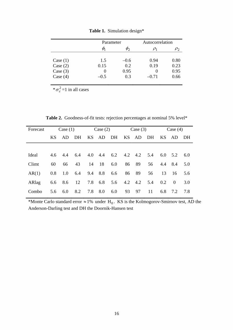
Table 1. Simulation design*

Parameter Autocorrelation 1φ 2φ 1ρ 2ρ Case (1) 1.5 –0.6 0.94 0.80 Case (2) 0.15 0.2 0.19 0.23 Case (3) 0 0.95 0 0.95 Case (4) –0.5 0.3 –0.71 0.66

* 2εσ =1 in all cases

Table 2. Goodness-of-fit tests: rejection percentages at nominal 5% level*

Forecast Case (1) Case (2) Case (3) Case (4)

KS AD DH KS AD DH KS AD DH KS AD DH

Ideal 4.6 4.4 6.4 4.0 4.4 6.2 4.2 4.2 5.4 6.0 5.2 6.0

Climt 60 66 43 14 18 6.0 86 89 56 4.4 8.4 5.0

AR(1) 0.8 1.0 6.4 9.4 8.8 6.6 86 89 56 13 16 5.6

ARlag 6.6 8.6 12 7.8 6.8 5.6 4.2 4.2 5.4 0.2 0 3.0

Combo 5.6 6.0 8.2 7.8 8.0 6.0 93 97 11 6.8 7.2 7.8

*Monte Carlo standard error under H . KS is the Kolmogorov-Smirnov test, AD the Anderson-Darling test and DH the Doornik-Hansen test

1%≈ 0

16

Table 3. Tests of independence: error autocorrelations and rejection percentages

Forecast Case (1) Case (2) Case (3) Case (4)

1( )eρ LB Bk 1( )eρ LB Bk 2( )*eρ LB Bk 1( )eρ LB Bk

Ideal 0 4.4 4.2 0 3.8 4.6 0 6.2 5.6 0 5.2 3.4

Climt .94 100 100 .19 68 53 .95 100 99 –.71 100 100

AR(1) .56 100 100 –.04 43 17 .95 100 99 .21 78 62

ARlag .77 100 100 .15 24 30 0 6.2 5.6 –.35 99 97

Combo .73 100 100 .06 16 14 .80 98 100 –.16 35 62

* 1 ( ) 0eρ = for all forecasts in Case 3. LB is the Ljung-Box test and Bk the likelihood ratio test of Berkowitz (2001)

Table 4. Additional evaluation criteria: KLIC and (negative) average logarithmic score

Forecast Case (1) Case (2) Case (3) Case (4)

KLIC –logS KLIC –logS KLIC –logS KLIC –logS

Ideal 0 142 0 142 0 142 0 142

Climt 128 270 3.83 145 117 258 39.6 182

AR(1) 22 164 2.04 144 117 258 4.8 147

ARlag 75 217 1.16 143 0 142 11.9 154

Combo 43 185 0.71 142 35 177 3.3 145

17