Evaluating Forecast Performance with State Dependence∗

Florens Odendahl1, Barbara Rossi2, and Tatevik Sekhposyan3

1Banco de España†2Universitat Pompeu Fabra, Barcelona GSE and CREI‡

3Texas A&M University§

July 18, 2021

Abstract

We propose a novel forecast evaluation methodology to assess models’ absolute and relativeforecasting performance when it is a state-dependent function of economic variables. Inour framework, the forecasting performance, measured by a forecast error loss function, ismodeled via a hard or smooth threshold model with unknown threshold values. Existingtests either assume a constant out-of-sample forecast performance or use non-parametric tech-niques robust to time-variation; consequently, they may lack power against state-dependentpredictability. Our tests can be applied to relative forecast comparisons, forecast encompassing,forecast efficiency, and, more generally, moment-based tests of forecast evaluation. MonteCarlo results suggest that our proposed tests perform well in finite samples and have betterpower than existing tests in selecting the best forecast or assessing its efficiency in the presenceof state dependence. Our tests uncover “pockets of predictability” in U.S. equity premia;although the term spread is not a useful predictor on average over the sample, it forecastssignificantly better than the benchmark forecast when real GDP growth is low. In addition, wefind that leading indicators, such as measures of vacancy postings and new orders for durablegoods, improve the forecasts of U.S. industrial production when financial conditions are tight.

Keywords: State dependence; Forecast evaluation; Predictive ability testing; Moment-basedtests; Pockets of predictability.JEL codes: C52, C53, E17, G17.

∗We thank Lukas Hoesch and the participants of the International Institute of Forecasters Macroeconomic Forecastingwebinar for useful comments and suggestions. The views expressed herein are those of the authors and should not beattributed to the Banco de España or the Eurosystem. This project has received funding from the European ResearchCouncil (ERC) under the European Union’s Horizon 2020 research and innovation programme (grant agreement No615608) and the Spanish Ministry of Economy and Competitiveness, Grant ECO2015-68136-P and FEDER, UE. TheBarcelona GSE acknowledges financial support from the Spanish Ministry of Economy and Competitiveness throughthe Severo Ochoa Programme for Centers of Excellence in R&D (SEV-2015-0063). Part of this project was completedwhile Florens Odendahl was employed at the Banque de France, while Tatevik Sekhposyan was a visiting fellow atthe Federal Reserve Bank of San Francisco and the authors would like to thank the respective institutions for theirassistance that made this research possible.†Address: Calle de Alcalá 48, 28014 Madrid, Spain. Email: florens.odendahl@bde.es.‡Address: c/Ramon Trias Fargas 25/27, 08005 Barcelona, Spain. Email: barbara.rossi@upf.edu.§Address: 4228 TAMU, College Station, TX 77843, USA. Email: tsekhposyan@tamu.edu.

1 Introduction

Decision-makers face an abundance of candidate forecasting models, and, starting with Dieboldand Mariano (1995) and West (1996), the literature has proposed a variety of forecast comparisontests to guide forecasters in choosing the model. However, usually, no single model emergesas the best overall; typically, the forecasting performance is prone to instabilities and, therefore,depends on the sample. One possible explanation is that the economic mechanisms that generatethe data are time-varying such that a given model is better in some periods and worse in others,resulting in a state-dependent (or more generally, non-linear) forecasting performance. Theseempirical findings also hold when evaluating the absolute forecasting performance.

In this paper, we propose a new forecast comparison test as well as, more generally, moment-based forecast evaluation tests (such as rationality, efficiency, and encompassing) that havepower against the alternative of state dependence in the forecasting performance. The statedependence is assumed to take the parametric form of a threshold model, i.e. the relativeforecasting performance is a non-linear function of an economic observable variable and arespective threshold. We consider both hard threshold models as well as logistic smooth thresholdand exponential smooth threshold models. Importantly, we allow the value of the thresholdto be unknown and estimate it alongside the testing procedure. Existing tests either focus onconstant relative out-of-sample performance (Giacomini and White, 2006) or use non-parametrictechniques to detect time-varying deviations from equal performance (Giacomini and Rossi, 2010;Amisano and Giacomini, 2007); we show that the latter approaches may lack power against thealternative of parametric state dependence.

Our paper is the first to model state dependence in the form of a hard or smooth thresholdmodel directly on the forecasting performance. While Hansen’s (1996b) test detects non-linearitiesin-sample, our test instead allows forecasters to evaluate the out-of-sample predictive ability when itmay be state-dependent. Testing in the presence of an unknown threshold requires non-standardstatistics since the nuisance parameter (the threshold) is present only under the alternative;therefore, the standard Wald, Likelihood ratio, and Lagrange multiplier tests do not have theusual asymptotic chi-square distribution (Davies, 1977, 1987). While in some cases there mightbe an economic justification for selecting an ad-hoc threshold value and treating it as known,this is not generally the case, and allowing for an unknown threshold makes our approachbroadly applicable. There are several differences between our approach and Hansen’s (1996b): forexample, when evaluating the relative forecasting performance (i) we apply the threshold modeldirectly to the relative predictive performance, measured by the forecast loss differential, and (ii)we test for a zero expected forecast performance differential, while Hansen (1996b) leaves theexpected value unspecified under the null hypothesis. Consequently, we jointly test whether theout-of-sample average relative forecasting performance is different from zero as well as whetherit is state-dependent.

While our focus is on the loss differential, the leading evaluation approach in applied work,our methodology more generally applies to other forecast evaluation tests that are implementedwith moment conditions. For instance, tests of efficiency and encompassing can be formulated interms of moment conditions.

We investigate the finite sample performance of our tests with Monte Carlo simulations. Our

1

simulations suggest, for example, that our proposed tests are well-sized and have better poweragainst the alternative of an unequal and state-dependent forecasting performance relative tothe existing tests. These results continue to hold even when the state variable is observed withmeasurement error (see in the Online Appendix).

There are several reasons why considering state dependence in the forecast error losses/lossdifferentials is interesting. First, it allows the forecaster to impose the null hypothesis directly onthe object of interest. While it is true that the researcher can potentially consider state dependencein the forecasting models directly, satisfactory in-sample fit does not necessarily translate tosatisfactory out-of-sample performance. Therefore, studying the object of interest (i.e. the forecasterror loss) directly is useful. Second, studying forecast error losses/loss differentials makes ourframework applicable to the case when the forecasting model is known as well as the case whenit is not known (as in widely used survey forecasts). Third, in the case of multivariate models ormodels with many predictors, the researcher faces the problem of selecting the predictors thatare state-dependent; this problem does not arise when directly studying the losses with respectto the target variable of interest. Last, parsimonious linear models are used extensively in theforecasting literature. Our tests allow us to evaluate these models against state dependence in atheoretically coherent framework. The test results guide the researcher on how to modify theoriginal forecasting models and their estimation technique, as well as on how to select models forprediction at a given point in time.

Our paper contributes to the recent literature on forecast evaluation (Diebold and Mariano,1995; West, 1996; Clark and McCracken, 2001; Clark and West, 2006, 2007; Giacomini and White,2006; Giacomini and Rossi, 2010). In particular, Giacomini and White (2006) (GW henceforth)show the validity of the asymptotic Normal distribution for the out-of-sample test of equalpredictive ability proposed by Diebold and Mariano (1995) (DM henceforth) when the underlyingforecasting models are estimated using a rolling window estimation scheme and the data satisfycertain mixing properties.1 Following their framework, our testing procedure similarly relies ona rolling window estimation scheme to preserve the parameter estimation error asymptotically.Hence, we compare forecasting methods rather than forecasting models. However, while GWfocus on the null hypothesis of an equal out-of-sample predictive ability, on average, our testallows for state dependence on the conditioning variables, i.e. we test for deviations from thenull hypothesis in sub-samples identified by state variables. Importantly, we do not require theconditioning variable itself to explain the forecasting performance (although it could) but only toindicate the state, i.e. the magnitude of the predictive ability within a state can be independentof the conditioning variable. Our paper is also related to Giacomini and Rossi (2010), whichallows the relative forecasting performance to be prone to instabilities, using a non-parametrictime-variation approach based on the rolling/recursive window estimation of a local GW test.As a result, their test has good power against smooth and persistent changes but, as we show, itmight lack power against the switches of a state-dependent model.

Several papers in the literature (Stock and Watson, 2009; Rapach et al., 2010; Neely et al., 2014;Dotsey et al., 2018; Granziera and Sekhposyan, 2019) evaluate forecast performance in subsamples,where the subsamples are identified conditional on some economic variable being smaller orlarger than an ad-hoc threshold. For instance, Stock and Watson (2009) analyze the forecasting

1Hereafter, we refer to the DM test under the conditions of Giacomini and White (2006) as the GW test.

2

ability of Phillips curve models for U.S. inflation and conclude, from plotting the loss differential,that the forecasting performance depends on the unemployment gap: “when the unemploymentgap exceeds 1.5 in absolute value, the Phillips curve forecasts improve substantially upon theUC-SV [unobserved component with stochastic volatility] model.” (Stock and Watson, 2009).Rapach et al. (2010) investigate equity return predictability during different states of the businesscycle by using the“good, normal, and bad times” classification of GDP growth from Liew andVassalou (2000). Our methodology, instead, systematically tests for potential state dependencewithout having to know or assume the threshold value.

We demonstrate the usefulness of our methodology in two empirical applications. First, wecompare models that predict U.S. equity premia from 1966 to 2011. As noted in Pesaran andTimmermann (1995) and Rapach and Wohar (2006), financial return predictability is typicallytime-varying and appears only in sub-samples.2 Instabilities in forecasting performances in otherfinancial variables are widespread as well: Paye and Timmermann (2006), for instance, cannotreject the presence of structural breaks in stock return predictive regressions and Rossi (2006,2013b) finds similar results for exchange rate returns. As summarized in Timmermann (2008),“... there appear to be pockets in time where there is modest evidence of local predictability;(...) the best forecasting method can be expected to vary over time, and there are likely to beperiods of model breakdown where no approach seems to work”. In our empirical results, we dofind evidence of state-dependent predictive ability. When forecasting stock market returns, weshow the usefulness of our test statistic for detecting pockets of predictability. Furthermore, ourapproach can shed light on which factors create such pockets. More in detail, our benchmarkmodel is an in-sample mean, re-estimated in real-time rolling windows, whereas the competitormodels use the financial variables from Welch and Goyal’s (2008) comprehensive dataset ofpredictors. We find evidence of state dependence in the relative forecasting performance, wherethe state dependence is a function of the business cycle, measured by the monthly real GDPgrowth estimate of Koop et al. (2020): in periods of above-average GDP growth, the economicmodel tends to underperform relative to the benchmark model. However, in periods of lowgrowth, forecasting with the term spread, defined as the difference between the long-term andthe T-bill yields, leads to forecast improvements. On the other hand, the GW and Fluctuation testscannot reject the null hypothesis of equal forecasting ability and fail to uncover such pockets ofpredictability.3 Our result that the spread is a useful predictor during times of low GDP growthis also in line with a recent study of Moench and Stein (2021), who reach a similar conclusionusing a very different approach.

Second, we evaluate U.S. industrial production forecasts from January 1971 to December 2019.The choice of our state variable, the adjusted National Financial Conditions Index (ANFCI) com-puted by the Chicago Fed, is motivated by the work of Adrian et al. (2019). They demonstrated theimportance of financial conditions for forecasting the distribution of output growth, particularlytail risk, advocating for a non-linear relationship between financial stability and macroeconomicperformance. We find that certain leading indicators such as measures of vacancy postings andnew orders for durable goods are particularly useful (relative to parsimonious autoregressivebenchmarks) for forecasting U.S. industrial production when financial conditions, measured by

2See Goyal and Welch (2003); Welch and Goyal (2008) for a related discussion.3Note that the forecasting gains using the financial predictors are small and that any large deviations from equal

predictive ability in favor of the economic models would imply strong violations of the rational expectations hypothesis.

3

the ANFCI, are tight.Our paper is further related to Harvey et al. (2021) and Inoue and Rossi (2015), who also

propose methodologies to study time-variation in predictive regressions. There are severaldifferences with their methodologies, however. As indicated before, our tests are designed forout-of-sample forecast evaluation, while Harvey et al. (2021) and Inoue and Rossi (2015) considertesting the significance of a specific predictor in-sample, which does not necessarily imply betterout-of-sample performance. Most importantly, our method allows the researcher to shed lighton the economic causes behind the changes in the models‘ predictive ability since the variationin the forecasting performance is linked to the economic variables that define the states. On theother hand, Harvey et al. (2021) and Inoue and Rossi (2015) propose a sequential procedure asopposed to the one-shot evaluation proposed in this paper. The sequential procedure is tailoredto monitor the predictive performance in real-time. Our one-shot procedure, on the other hand,evaluates the out-of-sample forecasting performance historically, yet still allows picking the bestperforming model depending on the identified state at the end of the sample.

The paper is organized as follows. Section 2 formalizes our null hypothesis, introduces ourtest statistics, and describes the challenges that arise when testing for state dependence in relativeforecasting performance. Section 3 evaluates the size and power of our proposed procedure infinite samples via Monte Carlo simulations. Section 4 investigates the existence of pockets ofpredictability in financial data and Section 5 investigates state dependence in the relative forecastperformance of models predicting U.S. industrial production. Section 6 concludes.

2 Testing for state dependence: methodology

We first describe the model and the null hypothesis. We further provide illustrative examples ofhow state-dependence in forecast losses can arise. Then, we introduce the necessary notation, thetechnical assumptions, and the test statistic.

2.1 The General framework

Let f (1)t+h|t(At, At−1, ..., At−R+1; β(1)t,R) and f (2)t+h|t(At, At−1, ..., At−R+1; β

(2)t,R) denote two measurable

functions, which provide the forecasts of two competing models, labeled (1) and (2), where tdenotes the forecast origin, h denotes the forecast horizon, and the vector of stochastic processesAt = (Yt, Zt) contains the variable of interest Yt and the column vector of predictors Zt. In turn,β(i)t,R denotes the vector of estimated parameters at time t of model “i”(i = 1, 2) using a rolling

window estimation scheme of size R ≤ R < ∞ and data At, ..., At−R+1.4 Henceforth, we simplywrite f (1)t+h|t and f (2)t+h|t. Importantly, note that the function f (i)t+h|t can denote either a point or a

density forecast. Finally, let f (i)t+h|t denote the forecast under the true but unknown parameter

value β(i).Let Lt+h|t

(Yt+h, f (i)t+h|t

)denote a loss function, which evaluates the prediction f (i)t+h|t of Yt+h.

The loss functions we allow for are quite general and encompass the quadratic loss (which givesrise to a Mean Squared Forecast Error, MSFE, measure of predictive ability), asymmetric losses(such as the lin-lin loss), as well as the log score and Continuous Rank Probability Score (CRPS)

4The window size R is assumed to be the same across the two models for notational convenience only.

4

for density forecasts. We define the forecast error loss of interest to the researcher as Lt+h|t. Notethat Lt+h|t denotes our object of interest, which can be different from the loss function Lt+h|t(·)itself. For instance, when the researcher is interested in the relative predictive ability under theMSFE loss function, Lt+h|t is the difference of the squared forecast errors; while in the case offorecast efficiency, Lt+h|t denotes the relevant moment condition. We describe this in more detail

below. Note that Lt+h|t is a function of the estimated parameters β(i)t,R and the rolling window size

R. As we assume that the parameters are estimated over a rolling and finite window size, the lossdifferential compares forecasting methods rather than forecasting models.

We allow the forecast error loss to evolve over time according to a non-linear model (Teräsvirta,2006):

Lt+h|t = X′tµ + X′tθ · G(St; ϕ) + ut+h, (1)

where Xt and St are explanatory variables, ϕ is a vector of parameters, ut+h is an error term andG(·) is allowed to be a non-linear function. In eq. (1), µ and θ denote the parameters of interest,the vector Xt is a k1 dimensional column vector that denotes economic observables and a constant,St denotes the economic observable that introduces the state dependence, ϕ denotes the unknownthreshold, ut+h is the error term. For the remainder, St is assumed to be a scalar. In Appendix A.2we discuss the possibility of several candidate variables for St and how to extend the testingprocedure to account for that. Potential serial correlation can be accounted for by including lagsof Lt+h|t, which are allowed, but not required, to also be a function of the threshold indicator. St

is a stochastic process, assumed to be continuous and allowed to be a subvector of Xt. Also notethat not all elements of Xt must enter the equation non-linearly.

The non-linear model in equation (1) allows for a wide range of models which includes time-varying parameter models as long as the time-variation is a parametric function of an observableSt. Note that our framework does not allow St to be unobservable; for example, this rules out thecase of Markov switching models which we separately discuss in Section 2.5. We also show inMonte Carlo simulations that our test has power in cases where only a noisy measure, St, of St isavailable; for instance, in the case where St is an estimate of the true but unobserved variable St.

In particular, the model classes we consider encompass several interesting cases for G(St; ϕ).The first case is a threshold regression (TR) model:

TR: G(St; ϕ) = 1 (St ≥ γ) , where ϕ = γ, (2)

i.e. the effect of Xt on Lt+h|t changes if St is above the threshold γ. The second case is the logisticsmooth threshold regression (LSTR) model:

LSTR: G(St; ϕ) =(1 + exp{−τ(St − γ)}

)−1, where ϕ = (γ, τ), (3)

with 0 < τ < ∞ and the effect of Xt on Lt+h|t changes smoothly if St is either above or below athreshold γ and the smoothness of the function is controlled by τ. The third case is an exponentialsmooth threshold regression (ESTR) model:

ESTR: G(St; ϕ) = 1− exp{−τ(St − γ)2}, where ϕ = (γ, τ), (4)

with 0 < τ < ∞ and the effect of Xt on Lt+h|t changes smoothly if St is either above or below a

5

threshold γ, where τ controls the smoothness of the change. We give more details below abouthow to choose the grid for γ. In the following, we refer to a smooth threshold regression model(STR) whenever the function G(·) has no discontinuity.

Figure 1 plots the functional forms of the TR, LSTR, and ESTR models. The TR and LSTRare similar, with the difference being that the LSTR is smooth and the TR has a kink at γ. Bothmodels are useful in cases where the delta losses change when the threshold indicator variableis larger (smaller) than γ. For instance, Rapach et al. (2010) find pockets of predictability forU.S. equity premia when U.S. GDP growth is low. The ESTR instead is most useful wheneverthreshold effects are present for deviations from an “equilibrium condition”, independently ofthe direction. For instance, Stock and Watson (2009) conclude from visual inspection that thePhillips curve model outperforms a benchmark model whenever the unemployment gap deviatesstrongly from its steady state value of zero, i.e. when the unemployment gap is particularly largeor small.

Figure 1: Functional forms of TR, LSTR, and ESTR

(a) TR vs. LSTR (b) TR vs. ESTR

Note: Panel (a) plots the LSTR, eq. (3), for two different values of τ against the TR, eq. (2). Panel (b) plots the ESTR, eq.(4), for two different values of τ against the TR. γ is set equal to zero in both plots. The y-axis denotes the functionvalue, G(St; ϕ). The x-axis denotes the value of St.

We aim at evaluating forecasting models’ predictive performance while being able to detectpossible additive non-linearities in the form of a hard or smooth threshold model. Our nullhypothesis of equal predictive ability at each point in time is:

E(Lt+h|t|Xt, St

)= 0 ∀t, (5)

versus the alternativeE(Lt+h|t|Xt, St

)= X′tµ + X′tθ · G(St; ϕ). (6)

The null and alternative hypotheses involve µ and θ and become H0 : µ = θ = 0 andHA : µ 6= 0, θ 6= 0 respectively. Note that the null hypothesis defined in eq. (5) holds conditionallyon Xt and St, and, therefore, by the law of iterated expectations, also unconditionally: E(Lt+h|t) = 0.Our test has power against either µ or θ or both jointly deviating from zero under the alternative,

6

i.e. either a constant non-equal predictive ability or a state-dependent (or non-linear) predictiveability or both.5 Importantly, we allow the nuisance parameter ϕ to be unknown. Therefore,testing for the null hypothesis described in equation (5) is subject to the problem of a nuisanceparameter that is present only under the alternative, which makes standard asymptotic inferenceinvalid (Davies, 1977, 1987; Hansen, 1996b).

Before describing our proposed test statistics, we want to emphasize two points. First, al-though the assumption of an unknown ϕ comes at the cost of non-standard inference, it bringsthe large benefit that it allows the researcher to test over a range of values, instead of having tochoose an arbitrary value. This is particularly important in practice because an ad-hoc choice forϕ can be detrimental to the power of detecting state dependence. In practice, when working withthe TR, LSTR or ESTR model, we recommend to formulate γ in terms of the empirical distributionfunction Ξn(·) of St such that the indicator becomes 1

(Ξn(St) ≥ γ

), with γ ∈ Γ = [0, 1] and

Ξ−1n (γ) provides the threshold in units of St (Hansen, 1996b). This is particularly useful when

implementing the model in statistical programs, as it allows formulating a unit-free grid for γ.Following Hansen (1996b) and others, we restrict γ to be away from the boundaries and choose,for instance, Γ = [0.15, 0.85]. Therefore, when we express the bounds of the threshold value interms of St, its lower and upper bounds are St = Ξ−1

n (0.15) and St = Ξ−1n (0.85) respectively. In

other words, restricting the values of γ to Γ = [0.15, 0.85] refers to the lower 15th and upper 85thpercentile of the empirical cumulative distribution function (cdf) of St; importantly, the restrictionof Γ = [0.15, 0.85] does not refer to a time index where we have to leave the endpoints out, i.e.detection of a change of the state is possible in real-time using our method.

Tests of equal predictive ability: Tests of equal predictive ability are implemented by letting

Lt+h|t = ∆Lt+h|t ≡ Lt+h|t

(Yt+h|t, f (1)t+h|t

)− Lt+h|t

(Yt+h|t, f (2)t+h|t

). (7)

The following specification of eq. (1) is of particular interest in the forecast comparison case, as itspecifies state dependence that is a function solely of St and does not depend on any additionalobservables Xt:

∆Lt+h|t = µ + θ · G(St; ϕ) + ut+h. (8)

The specification in eq. (8) contains as special cases the standard Diebold and Mariano (1995) andGiacomini and White (2006) tests for equal predictive ability, and, unlike the latter, is capable ofdetecting periods of unequal performance that depend on St in a non-linear fashion.

Tests of forecast encompassing: While our leading case is the loss differential, as it is widelyused in applied work, our methodology can also be applied to the moment conditions of forecastencompassing tests. Let εt+h|t,1 = Yt+h − f (1)t+h|t and εt+h|t,2 = Yt+h − f (2)t+h|t. To test whether model(1) encompasses model (2), we define

Lt+h|t = ENCt+h|t ≡ ε2t+h|t,1 − εt+h|t,1εt+h|t,2. (9)

Then, to test our null hypothesis that the forecast of model one encompasses the forecast of

5Note that the case of µ = θ 6= 0 is a valid alternative and merely represents the joint presence of a non-equal andnon-linear predictive ability.

7

model two, the following specification is of particular interest:

ENCt+h|t = µ + θ · G(St; ϕ) + ut+h. (10)

As in the case of the loss differential in eq. (8), the null and alternative hypothesis in the forecastencompassing test in eq. (10) involve µ and θ and become H0 : µ = θ = 0 and HA : µ 6= 0, θ 6= 0respectively.

Tests of forecast optimality: Tests of forecast optimality include tests of forecast unbiasednessand efficiency. In those cases, only the forecast error loss of one model is evaluated (e.g. modeli). Tests of forecast unbiasedness and forecast efficiency, respectively, can be formulated as amoment-based test by defining

Lt+h|t = UBt+h|t ≡ yt+h − f (i)t+h|t and Lt+h|t = FEt+h|t ≡(yt+h − f (i)t+h|t

)· f (i)t+h|t, (11)

and can be tested using the specification:

UBt+h|t = µ + θ · G (St; ϕ) + ut+h and FEt+h|t = µ + θ · G (St; ϕ) + ut+h. (12)

In both cases, the null hypothesis of unbiasedness and efficiency, respectively, is implementedby µ = θ = 0. In the Online Appendix, we show Monte Carlo simulation results for forecastefficiency tests.

2.2 Examples of thresholds in the loss differential

In this subsection, we discuss two simple analytical examples of how threshold-type effects in thelosses can arise.

Example one: A first example is based on a DGP that includes a common component. Inparticular, two observable variables, yt and xt, are driven by a common component, ct, andunpredictable idiosyncratic components, et and ηt, respectively:

yt+1 = α + ct+1 + et+1, xt+1 = ct+1 + ηt+1, ct+1 = ρct + vt+1, (13)

where α is a constant, et+1 ∼iid N(0, σ2e ), ηt+1 ∼iid N(0, σ2

η), the subscript iid denotes inde-pendently and identically distributed random variables, and |ρ| < 1. Importantly, vt+1 ∼N(0, σ2

v,t+1), i.e. it is an independent variable and the variance is time-varying with σ2v,t+1 =

σ2v,1 + G(St+1; ϕ)σ2

v,2, where σv,1, σv,2 > 0, and σ2v = E(v2

t ) is the unconditional variance of vt.St ∼iid N(0, 1) determines the variance of the shocks to the common component and since σ2

v,t+1

is unobservable, St+1 is a proxy variable that is indicating the strength of the common component.Let the two forecasts (calculated using the true parameter values) be

f (1)t+1|t = α and f (2)t+1|t = α + ρxt. (14)

Note that, unconditionally, E(c2t ) = σ2

v /(1− ρ2). We start by considering the case where thereis no parameter estimation error such that the forecast error is given by εt+1|t,i = yt+1 − f (i)t+1|t.

8

Then, the unconditional expected value of the squared forecast error difference takes the form

E[ε2t+1|t,1 − ε2

t+1|t,2] = ρ2σ2v /(1− ρ2)︸ ︷︷ ︸

misspecification of model one

− ρ2σ2η .︸ ︷︷ ︸

misspecification of model two(15)

In other words, if the models are equally misspecified, their expected squared forecast errordifference is zero.

Conditionally on St, we have that

E[ε2t+1|t,1 − ε2

t+1|t,2|St] = ρ2(σ2v /(1− ρ2)− σ2

η)︸ ︷︷ ︸unconditional difference

+ ρ2(σ2v,1 + G(St; ϕ)σ2

v,2 − σ2v )︸ ︷︷ ︸

state-dependent difference

,(16)

i.e. the conditional expected squared forecast error difference is a non-linear function of St,independently of the expected value of the unconditional squared forecast error difference. Inother words, eq. (16) exemplifies how a loss differential with the dynamics proposed in eq. (8)can arise.

In practice, the parameter estimation error affects forecast errors: let εt+1|t,i = yt+1 − f (i)t+1|tdenote the forecast error when parameters are estimated. In this case, we obtain the followingexpected loss differential:

E(∆Lt+1|t) =E[ε2t+1|t,1 − ε2

t+1|t,2] = ρ2(σ2v /(1− ρ2)− σ2

η)︸ ︷︷ ︸due to misspecification

+Παt,R,(1)−Παt,R,(2)

−Πρt,R,(2)︸ ︷︷ ︸due to parameter estimation error

,(17)

where Παt,R,(1)captures the contribution of the parameter estimation error6 associated with the

estimated constant of model (1) to the expected loss differential, and Παt,R,(2)and Πρt,R,(2)

capturethe contribution of the parameter estimation error of the estimated constant and the slopeparameter of model (2); the expressions for Παt,R,(1)

, Παt,R,(2), and Πρt,R,(2)

are given in the OnlineAppendix.

The expected value of the loss differential is now a function of the relative model misspecifica-tion as well as the parameter estimation error. For instance, a larger misspecification of model(1), σ2

v /(1− ρ2) > σ2η , can be compensated by a relatively smaller contributions of the parameter

estimation error, Παt,R,(1)< Παt,R,(2)

+ Πρt,R,(2), such that the expected loss differential is equal to

zero.The expected value of the loss differential, conditionally on St, is then

E(∆Lt+1|t|St) =ρ2(

σ2v /(1− ρ2)− σ2

η

)+ ρ2

(σ2

v,1 + G(St; ϕ)σ2v,2 − σ2

v

)+ Π(St)

αt,R,(1)−Π(St)

αt,R,(2)−Π(St)

ρt,R,(2)+ Π(⊥St)

αt,R,(1)−Π(⊥St)

αt,R,(2)−Π(⊥St)

ρt,R,(2),

(18)

where the superscripts (St) and (⊥ St) denote dependence on and independence of St, respec-tively. Note that while the first line of eq. (18) is necessarily different from zero for some valuesof St, the terms of the parameter estimation error in the second line may dampen or amplifythis effect. In particular, if Π(⊥St)

αt,R,(1)−Π(⊥St)

αt,R,(2)−Π(⊥St)

ρt,R,(2)is large relative to the other terms in eq.

6The component capturing the contribution of the parameter estimation error also contains the covariance of theparameter estimation error and the misspecification.

9

(18), the effect of the state-dependence on the expected loss differential could be small. In turn,if Π(⊥St)

αt,R,(1)−Π(⊥St)

αt,R,(2)−Π(⊥St)

ρt,R,(2)is small relative to the other terms in eq. (18), the effect of state-

dependence on the expected loss differential remains large after taking the parameter estimationerror into account.

Example two: As a second example, consider the following DGP:

yt+1 = α + φzt + βG(St; ϕ)xt + et+1, (19)

with et+1 ∼iid N(0, σ2e ), zt ∼iid N(0, σ2

z ), and xt ∼iid N(0, σ2x). St and ϕ are the indicator variable

and parameters that govern the non-linear function G(·). The two competing forecasts (calculatedusing the true parameter values) are:

f (1)t+1|t = α + φzt and f (2)t+1|t = α + φzt + βxt. (20)

In this framework, the variable xt enters non-linearly in the DGP, as a function of St and ϕ, butthe non-linear relationship is not accounted for in the forecasting model.

Again, we start by considering the case where there is no parameter estimation error suchthat the squared forecast error of model one, ε2

t+1|t,1, minus the squared forecast error of modeltwo, ε2

t+1|t,2, is:

E[ε2t+1|t,1 − ε2

t+1|t,2] = β2σ2xE[G2(St; ϕ)]︸ ︷︷ ︸

misspecification of model one

− β2σ2xE[G2(St; ϕ)] + 2β2σ2

xE[G(St; ϕ)]− β2σ2x︸ ︷︷ ︸

misspecification of model two

= 2β2σ2xE[G(St; ϕ)]− β2σ2

x︸ ︷︷ ︸due to misspecification

,(21)

such that E[ε2t+1|t,1− ε2

t+1|t,2] is a function of St and ϕ. The term 2β2σ2xE[G(St; ϕ)]− β2σ2

x measureswhether including xt as a linear predictor in the model improves the expected forecastingperformance relative to a model without xt. For instance, if G(St; ϕ) = 1 (St ≥ γ), with ϕ = γ,then if E[St ≥ γ] = 0.5 we have that E[ε2

t+1|t,1 − ε2t+1|t,2] = 0, i.e. the models forecast equally well

in expectations. However, if E[St ≥ γ] > 0.5 it follows that E[ε2t+1|t,1 − ε2

t+1|t,2] > 0, i.e. modeltwo has a lower expected squared forecast error. This is because xt is present in the DGP morethan half of the time and, therefore, xt is a useful predictor despite the linear misspecification.Conditionally on St we have

E[ε2t+1|t,1 − ε2

t+1|t,2|St < γ] = −β2σ2x and E[ε2

t+1|t,1 − ε2t+1|t,2|St ≥ γ] = β2σ2

x , (22)

i.e. the loss differential is a threshold function of St and γ. In the case of forecast encompassing,the moment condition takes the form:

E[ε2t+1|t,1 − εt+1|t,1εt+1|t,2] = β2σ2

xE[G(St; ϕ)], (23)

which is again a non-linear function of St and ϕ.

10

Again, in practice the parameter estimation error affects the expected loss:

E(∆Lt+1|t) =E[ε2t+1|t,1 − ε2

t+1|t,2]

= 2β2σ2x E[G(St; ϕ)]− β2σ2

x︸ ︷︷ ︸due to misspecification

+Παt,R,(1)+ Πφt,R,(1)

−Παt,R,(2)−Πφt,R,(2)

−Πβt,R,(2),︸ ︷︷ ︸

due to parameter estimation error

(24)

where Παt,R,(1)and Πφt,R,(1)

capture the contribution of the parameter estimation error, associatedwith the estimated constant and the slope coefficient of model (1), to the expected loss differential,and Παt,R,(2)

, Πφt,R,(2), and Πβt,R,(2)

capture the contribution of the parameter estimation error of theestimated constant and the slope coefficients of model (2); their exact expressions are given in theOnline Appendix. As in the first illustrative example, the expected value of the loss differentialis a function of the relative model misspecification as well as the parameter estimation error.The mean squared forecast error differential due to the misspecification of model (2) can becompensated by the relative contributions of parameter estimation errors from the two models tothe MSFEs, such that the expected loss differential is equal to zero.

Continuing the example with G(St; ϕ) = 1 (St ≥ γ), conditionally on St we have

E(∆Lt+1|t|St < γ) = −β2σ2x + Παt,R,(1)

+ Πφt,R,(1)−Παt,R,(2)

−Πφt,R,(2)−Πβt,R,(2)

(25)

andE(∆Lt+1|t|St ≥ γ) = β2σ2

x + Παt,R,(1)+ Πφt,R,(1)

−Παt,R,(2)−Πφt,R,(2)

−Πβt,R,(2). (26)

Although the parameter estimation error, in this example, does not depend on St, it affects theconditional expected loss differential. However, as long as the parameter estimation error is notlarge relative to β2σ2

x , the state-dependence in the expected loss differential will be importantwhen testing for an equal predictive ability of model (1) and (2).

2.3 Test statistics

The parameter vector ϕ is an element of the compact set Φ which is a bounded subset of Rq. LetQt(ϕ) be a k-dimensional column vector that contains the explanatory variables of the threshold

model described in eq. (1), i.e. Qt(ϕ) =[

X′t,(Xt · G(St; ϕ)

)′]′, and let Qt = supϕ∈Φ |Qt(ϕ)|. Let

ψ(ϕ) =[µ(ϕ)′, θ(ϕ)′

]′ denote the vector of OLS parameter estimates under the alternative, andlet ut+h = Lt+h|t − Qt(ϕ)′ψ(ϕ) denote the error term under the alternative. The score underthe alternative is then given by st+h(ϕ) = Qt(ϕ)ut+h(ϕ). Let Hr denote a restriction matrix thatcorresponds to the null hypothesis defined in eq. (5). For instance, for the model described ineq. (8) without any additional regressors, we have that Hr = I2, where I2 is a two-dimensionalidentity matrix.7 Let T denote the total sample size and P = T − R− h denote the out-of-samplesize, i.e. the number of observations of Lt+h|t. Let VP(ϕ) = 1

P ∑T−ht=R st+h(ϕ)st+h(ϕ)′ denote the

variance-covariance matrix of the score, let V(ϕ) = E(st+h (ϕ) st+h (ϕ)′

)be finite and positive

definite for st+h (ϕ) = Qt(ϕ)ut+h, and let V∗P (ϕ) = MP(ϕ, ϕ)−1VP(ϕ)MP(ϕ, ϕ)−1 be the robustestimator of the variance-covariance matrix of ψ, with MP(ϕ1, ϕ2) = 1

P ∑Tt=R−h Qt(ϕ1)Qt(ϕ2)′,

and M(ϕ1, ϕ2) = E(Qt(ϕ1)Qt(ϕ2)′

); also, let KP(ϕ1, ϕ2) =

1P ∑T−h

t=R st+h(ϕ1)st+h(ϕ2)′.

7If eq. (1) contains additional control variables, such as lags of Lt+h|t, that are not part of the forecast comparisonnull hypothesis, the restriction matrix will not be equal to an identity matrix.

11

We consider the following test statistics, based on Hansen (1996b) and Andrews and Ploberger(1994), which we collectively refer to as the DMNL test:

DMNL: gΦ(WP) =

supϕ∈Φ WP(ϕ) (“sup-W”)∫

Φ WP(ϕ)dw(ϕ) (“ave-W”)ln( ∫

Φ exp( 12WP(ϕ))dw(ϕ)

)(“exp-W”)

(27)

where w(ϕ) is a weighting function8 over ϕ ∈ Φ, ln(·) denotes the natural logarithm and WP(ϕ)

is defined asWP(ϕ) = Pψ(ϕ)′Hr

[H′rV

∗P (ϕ)Hr

]−1H′rψ(ϕ). (28)

Henceforth, we let gΦ(WP)

denote either of the three above mentioned functions, i.e. sup-W,exp-W, and ave-W.

Establishing the uniform convergence of our test statistic requires an empirical process centrallimit theorem (CLT) such that: (i) the regression score, st+h(·), is unbounded (since, for instance,ut is unbounded) and, (ii), functional forms for G(·; ϕ) are allowed to be non-smooth in ϕ (sincewe include a threshold model which is discontinuous around the threshold). As pointed out byAndrews (1993) and Hansen (1996b,c), the work of Doukhan et al. (1995) provides an adequateempirical process CLT. Other work, for instance, Andrews (1991) and Hansen (1996c), do notrequire strict stationarity but impose smoothness conditions on the function G(·; ϕ) that areviolated by the discontinuity of the threshold model. In turn, that means that the regularityconditions stated below are somewhat stricter than required for the smooth threshold modelssince both Andrews (1991) and Hansen (1996c) provide milder assumptions for an empiricalprocess CLT of smooth functions G(·; ϕ). We derive the limiting distribution of DMNL under thefollowing assumptions:

Assumption A1 (i) (At, Xt, St) is strictly stationary and absolutely regular with mixing coefficientsη(m) = O(m−δ) for some δ > v/(v− 1) and v > 1. (ii) The estimation window size, R, is finite and theestimation scheme is a rolling window estimation.

Assumption A2 For r > v > 1, E|Qt|4r < ∞, E|ut|4r < ∞, and infϕ∈Φ det(

M(ϕ, ϕ))> 0.

Assumption A3 (i) Let ξt(ϕ) ≡ X′tG(St; ϕ); for some B < ∞ and λ > 0,∣∣∣∣(ξt(ϕ1)− ξt(ϕ2)

)ut+h

∣∣∣∣ <B∣∣∣∣ϕ1 − ϕ2

∣∣∣∣λ. (ii) MP(ϕ1, ϕ2) and KP(ϕ1, ϕ2) converge almost surely to M(ϕ1, ϕ2) and K(ϕ1, ϕ2),uniformly in ϕ1, ϕ2 ∈ Φ.

Assumption A4 f (i)t+h|t(.) is a measurable function of lags of At, for i = 1, 2.

A1 limits the dependence and time-variation allowed in the loss differential under the null. A2ensures that the explanatory variables in eq. (1) has more than 4r finite moments and that thevariance-covariance matrix of Xt and St is non-singular for all ϕ. A3 (i) imposes a continuityassumption on the element of the score associacted with the non-linear function G(·), and A3(ii) ensures uniform convergence of MP(·) and KP(·) over ϕ ∈ Φ. A4 is an assumption on thefunctional form of the forecast itself, and ensures measurability of Lt+h|h. Then, the asymptoticdistribution in eq. (27) can be described as follows.

8Throughout the paper we use an equal weighting, i.e. w(ϕ) = ϕ.

12

Proposition 1 Let gΦ(Wp) be either supϕ∈Φ WP(ϕ),∫

Φ WP(ϕ)dw(ϕ) or ln( ∫

Φ exp( 12WP(ϕ))dw(ϕ)

),

where Φ is compact and WP(ϕ) = Pψ(ϕ)′Hr[H′rV∗P (ϕ)Hr

]−1H′rψ(ϕ), and ψ (ϕ) =[µ (ϕ)′ , θ (ϕ)′

]′is estimated from eq. (1). Then, under A1 to A4 and H0 defined in eq. (5): E

(Lt+h|t

)= 0 for all

t = R + h, ..., T andlim

P→∞gΦ(WP)→d

gΦ(χ2), (29)

where χ2 is a chi-square distribution with degrees of freedom rank(Hr), and gΦ(χ2) can be completely

characterized by its covariance kernel K(ϕ1, ϕ2). The test rejects H0 defined in eq. (5) when gΦ(WP)> φα,

where φα is the critical value (for a nominal size of α) that can be simulated according to Algorithm 1 below.

The proof of Proposition 1 is provided in Appendix A.1.

2.4 Practical implementation

The asymptotic distribution in eq. (29) is not nuisance parameter free and cannot be tabulatedexcept for special cases.9 Therefore, we follow Hansen (1996b) to propose an algorithm that canbe used to simulate the critical values and which we report here for the readers’ convenience.Loss differentials may exhibit serial correlations since it is a function of forecast errors, which areserially correlated for h > 1. To deal with potentially unaccounted serial correlation in the lossdifferential, i.e. an autocorrelated ut+h in eq. (1), we adjust the original algorithm for simulatingthe asymptotic distribution proposed by Hansen (1996b). The adjustment is based on a suggestionof Hansen (1996a).

Simulation Algorithm 1 Let st+h(ϕ), MP(ϕ, ϕ), V∗P (ϕ), and Hr be as defined in Section 2.3. LetB = (4(P/100)(2/9) + 1) be the bandwidth parameter of the Bartlett kernel used in the simulationalgorithm. Then, for each j = 1, ..., J do the following steps:

1. Draw a set of standard Normal random variates {vt,j}T−h+Bt=R :

(a) Calculate λjP(ϕ) = 1√

P1√

1+B ∑Bb=0 ∑T−h

t=R st+h(ϕ)vt+b,j;

(b) Calculate W jP(ϕ) = λ

jP(ϕ)′MP(ϕ, ϕ)−1Hr

[H′rV∗P (ϕ)Hr

]−1H′r MP(ϕ, ϕ)−1λjP(ϕ);

(c) Repeat (a)-(b) for all ϕ ∈ Φ;

2. Compute gjP = gΦ

(W j

P).

After J iterations, we obtain a set of {gjP}

Jj=1 draws from the conditional distribution of the test

statistic; the approximate critical values are obtained by calculating the relevant quantiles.

For instance, for the case of the threshold model with G(St; ϕ) = 1(St ≤ γ) the algorithmiterates over different values of γ ∈ Φ. In the case of a smooth threshold model, the algorithmiterates over different values of the pair ϕ = (γ, τ) ∈ Φ.

The adjustment for serial correlation in the simulation of the asymptotic distribution doesnot specify a specific process for the serial correlation and is, therefore, suited for a variety ofpossible autocorrelations structures in the loss differential. If the researcher has reason to believe

9See Hansen (1996b) for a discussion.

13

that there is no autocorrelation, for instance, in the case of h = 1, she can set B = 0 which reducesSimulation Algorithm 1 to the original algorithm proposed in Hansen (1996b).

Our analysis focuses on a loss differential approach to formally test predictive ability. Thereason why we focus on the loss differential is because our goal is to directly evaluate the out-of-sample performance of the forecasts based on the loss function preferred by the researcher. Thereare several advantages in working directly with the loss function approach to model evaluation,as opposed to testing the model’s parameters. One advantage is that in our framework we candirectly analyze the predictive performance even when the underlying forecasting models areunknown, for instance, in the case of using survey data, Greenbook forecasts, or the forecastspublished by institutions. A second advantage is that estimating a threshold regression requiressome potentially complicated choices regarding the model specification. For instance, in a modelwith many predictors, the researcher has to decide which variable is subject to the threshold effectand which one isn’t. This problem does not arise when testing for non-linearities directly in theforecast error losses.

When our test rejects the null hypothesis, it is important to analyze why: this could be due toeither the fact that a model performing worse/better while the performance of the other modelremained the same, or that both models forecasting performance deteriorated/improved. Tofurther investigate the reasons behind the time-varying performance, the researcher can computethe MSFE of each model in the different regimes identified via our methodology. Then, he/shecan compute the overall ratio of the MSFEs of the two competing models, as well as ratios in therespective sub-samples identified by our test. While not a formal test, this provides evidence toanswer the questions posed above: did one model get worse, or both models but one less so, ordid one model get better and the other worse. We discuss such an approach in the Monte Carlosimulations in Section 3.

2.5 State dependence via Markov switching

An alternative approach to model state dependence is Markov switching (Hamilton, 1989). Unlikethe threshold model, the regime changes in the Markov switching model depend upon anunobserved (latent) Markov chain, St. Testing in the presence of Markov switching also requiresnon-standard statistics as it is subject to two problems. The first problem is again the presence ofnuisance parameters that are only identified under the alternative; in this case, the state-to-statetransition probabilities and the coefficients that switch. The second problem is that, under the null,the score of the restricted parameters is identically zero, which violates the regularity conditionsthat are imposed to derive the asymptotic chi-square distribution of the finite-dimensional LR(Wald, LM) statistic by a first-order approximation. Therefore, the procedure proposed in Hansen(1996b), which deals with a nuisance parameter present only under the alternative, does notreadily apply to the case of Markov switching models. Instead, Hansen (1992); Garcia (1998); Choand White (2007); Carrasco et al. (2014) and Qu and Zhuo (2020) provide a variety of solutionsthat address both problems.

We propose a test for predictive ability in the presence of Markov switching based on Carrascoet al. (2014) in the Online Appendix and investigate its size properties as well. However, thetest, like all the tests for Markov switching listed above, relies crucially on a correctly specified

14

distribution under the null hypothesis.10 A misspecified likelihood under the null will generallylead to size distortions. For instance, consider the case where the true but unknown distributionis a Student’s t with no Markov switching. The researcher assumes a Gaussian distribution withno Markov switching under the null and a Markov switching model with regime dependent,conditional Gaussian distributions under the alternative. Then, despite the absence of Markovswitching in the data generating process, the mixture property of the Markov switching modelunder the alternative may approximate the Student’s t distribution better than the Gaussianmodel under the null hypothesis. Unreported results show that this leads to an over-rejection ofthe null hypothesis of no Markov switching.

While the assumption of Normality may be justified when applying tests for Markov switchingmodels directly on economic observables, the distribution of a loss differential is generallyunknown and may exhibit fatter tails than a Normal distribution (e.g. when using a quadratic loss).Consequently, the above-described problem is more severe in the case of forecast comparisons,and testing for Markov switching in this framework may be very sensitive to the choice of theparametric distribution. In contrast, and as outlined in Section 2.3, threshold models do not relyas heavily on the parametric assumptions on the error terms ut, and testing is, therefore, morerobust in practice.

3 Monte Carlo simulation analysis

In this section, we explore the size and power of our proposed tests in a series of Monte Carlosimulation exercises. We consider both nested and non-nested forecasting models as well as avariety of data generating processes (DGPs).

First, in Section 3.1 we investigate the size of our proposed DMNL tests for point forecasts. Weconsider threshold, logistic smooth threshold as well as exponential smooth threshold regressionspecifications. Additional size results for alternative DGPs as well as density forecasts can befound in Appendix B.1. We also consider forecast encompassing as well as moment-based tests offorecast efficiency in Appendix B.2 and in the Online Appendix, respectively. In all cases, thetests are well-sized for moderate sample sizes.

In Section 3.2, we focus on the power properties of the tests. We consider both cases wherethe specification of the loss differential under the alternative is aligned with the true DGP as wellas situations where it is not. For example, we let the true relative forecasting ability evolve overtime according to a threshold model; however, in one case the researcher specifies a thresholdmodel in the loss differential, and thus the specification under the alternative is aligned with theDGP, while in a second case the researcher specifies a smooth logistic threshold model, in whichcase the alternative and the DGP are not aligned. We also consider situations where the true DGPinvolves constant deviations from equal predictive ability.

While Section 3.1 and Section 3.2 consider DGPs directly modeled on the forecast error losses,in Section 3.3 we consider DGPs where the non-linear behavior in the forecast loss is generatedfrom a primitive specification of the true underlying data, which allows us to consider bothnested and non-nested forecasting models.

10Under the assumption of normality, the power of the test of Carrasco et al. (2014) relies on serial correlation in theerror terms, instead of other deviations from the distribution specified under the null.

15

Finally, in all the power exercises in the main paper, we consider the case in which the stateSt is observed. However, our test also has power in case the researcher only observes a noisyestimate of St — for example, when St is a latent variable. As we discuss in Section 3.1 andSection 3.2, our results are robust to situations in which the true state is unobserved and only anoisy estimate is available.

The horizon we consider is one (h=1), and the number of Monte Carlo replications is 3,000.For all Monte Carlo results we specified γ ∈ [0.15, 0.85], denoted in terms of the the empirical cdfof St, and τ ∈ [0.1, 5]. Results are not sensitive to reasonable changes in the domain of γ and τ.

3.1 Size results

The underlying data for the point forecast comparison are generated by

yt+1 = ν + δ1zt,1 + δ2zt,2 + et+1, (30)

where ν = δ1 = δ2 = 1, et ∼iid N(0, 1), zt,1 ∼iid N(0, 1), and zt,2 ∼iid N(0, 1). The parametervector β

(j)t = [νt,j, δt,j] denotes the OLS estimator β

(j)t =

(∑t

i=t−R+1 z(j)′

i−1z(j)i−1

)−1∑t

i=t−R+1 z(j)′

i−1yi,

where z(j)t = [1, zt,j]. The two point forecasts, both of which are misspecified, are denoted by:

f (1)t+1|t = z(1)t β(1)t , and f (2)t+1|t = z(2)t β

(2)t . As the misspecification of the two models is symmetric, it

is straightforward to show that they have the same predictive ability in expectation. That is, theloss differential, given by

∆Lt+1|t =(yt+1 − f (1)t+1|t)

2 − (yt+1 − f (2)t+1|t)2, (31)

is zero in expectation: E(∆Lt+1|t) = 0 for all t = R + 1, ..., T.We generate time series of ∆Lt+1|t based on eq. (31) for several values of R and P: R =

[25, 50, 100] and P = [50, 100, 200, 1000]. Then, we estimate the following model on the lossdifferential to investigate size:

∆Lt+1|t = µ + θ · G(St; ϕ) + ut+1, (32)

where G(·) indicates the functional form of the TR, LSTR or ESTR models, described in eq. (2),(3), and (4); St ∼iid N(0, 1) and we treat ϕ as unknown.

Table 1 shows results for point forecast comparison for the null hypothesis defined in eq. (5)for the three different test statistics: sup-W, exp-W, and ave-W. The size results are very similarfor the TR, ESTR, and LSTR specifications. Overall, the ave-W has the best size properties anddelivers size results that are good for P > 50 and R > 25 for both the threshold model and thesmooth threshold model(s). The results of the exp-W test are similar to the ave-W; however, sizedistortions are slightly bigger in small samples than in the ave-W case. While the sup-W testworks well in large samples (P > 100), it somewhat over-rejects in smaller samples. The fact thatthe ave-W has the smallest size-distortions and that the exp-W has smaller size distortions thanthe sup-W is a property also present in the original test of Hansen (1996b), who found similarresults in a small Monte Carlo study for his null hypothesis.11

11In an unreported Monte Carlo study, we confirm the finding that in the original test of Hansen (1996b), the smallestempirical rejection frequencies tend to be found for the ave-type test and the largest for the sup-type test.

16

Table 1: Size results from a comparison of point forecasts

Panel A. ave-W

TR ESTR LSTRR/P 50 100 200 1000 50 100 200 1000 50 100 200 1000

25 0.099 0.074 0.072 0.063 0.097 0.077 0.066 0.065 0.098 0.070 0.069 0.06150 0.102 0.073 0.071 0.062 0.092 0.072 0.070 0.056 0.101 0.081 0.073 0.055100 0.103 0.069 0.060 0.059 0.097 0.069 0.065 0.056 0.096 0.078 0.069 0.054

Panel B. exp-W

TR ESTR LSTRR/P 50 100 200 1000 50 100 200 1000 50 100 200 1000

25 0.112 0.072 0.067 0.062 0.099 0.077 0.064 0.055 0.103 0.072 0.069 0.05950 0.118 0.083 0.066 0.059 0.105 0.069 0.077 0.055 0.103 0.085 0.071 0.056100 0.118 0.074 0.063 0.057 0.105 0.073 0.060 0.056 0.101 0.076 0.070 0.052

Panel C. sup-W

TR ESTR LSTRR/P 50 100 200 1000 50 100 200 1000 50 100 200 1000

25 0.126 0.081 0.065 0.062 0.124 0.084 0.061 0.058 0.111 0.078 0.068 0.05750 0.140 0.090 0.071 0.060 0.126 0.081 0.072 0.059 0.103 0.091 0.073 0.059100 0.142 0.079 0.066 0.058 0.134 0.080 0.063 0.050 0.114 0.074 0.066 0.053

Note: The table displays empirical rejection frequencies of the null hypothesis H0 : µ = θ = 0 for the DMNL test for pointforecasts evaluated with the MSFE loss function. The nominal size is 5%. Panels A to C show the results for the ave-W,exp-W, and the sup-W for the threshold model (TR), and the smooth threshold model using an exponential (ESTR) and alogistic (LSTR) function. The results are based on 3,000 Monte Carlo replications.

As previously mentioned, size results for nested models and density forecasts, as well asmoment-based tests (such as forecast encompassing and efficiency), are discussed in Appendix B.1,Appendix B.2, and the Online Appendix, respectively.

3.2 Power results

In this section, we investigate the power properties of the threshold and logistic smooth thresholdregression models. In particular, we specify three different alternatives for the loss differentialdefined in equation (31). The first alternative investigates the power of the proposed test statisticsfor detecting state dependence (θ 6= 0). The second alternative investigates the empirical rejectionfrequency when both µ 6= 0 and θ 6= 0. The third alternative investigates power against a constantdeviation from the null of equal predictive ability (µ 6= 0).

In order to conduct the power analysis we proceed as follows. Let ∆L(0)t+1|t be the loss

differential obtained from one Monte Carlo draw of eq. (31), normalized by its sample standarddeviation (to ensure that the magnitude of the alternative is constant relative to the variation in∆Lt+1|t). For all simulations we use St ∼i.i.d. N(0, 1) and γ = 0.12 In particular, we define the lossdifferential under the first alternative, Alternative (1), as

∆L(1)

t+1|t(c) = ∆L(0)t+1|t + µc + θc · 1(St ≥ γ), (33)

12Note that St is re-drawn in each Monte Carlo iteration for each alternative; we suppress the respective subscriptsfor notational convenience.

17

where c = 1, 2, ..., 14 with µ1 = 0, µ2 = 0.085, µ3 = 0.170, ..., µ14 = 1.10, and θc = −2µc. Note thatγ = 0 implies that E(St ≥ γ) = 1

2 . Therefore, it follows that Et∆L(1)

t+1|t = µc + E(St ≥ γ)θc =

µc − 12 2µc = 0, i.e. the overall sample has a zero mean and the magnitude of the state-switching

coefficient is 0.17 times the standard deviation of ∆L(0)t+1|t, and so forth. In the case where c = 1,

µ1 = θ1 = 0 implies that the joint null, defined in equation (5), holds. The design of Alternative(1) aims at isolating the power against the threshold alternative only, i.e. keeping the expectedvalue over the full sample at zero. This enables us to compare the power of our tests to thepower of the existing Fluctuation and GW test under non-linear alternatives. Therefore, we setthe parameter values as described above to leave the expected value of the ∆L(1)

t+1|t(c) over the fullsample at zero.

For Alternative (2), the values of µc are unchanged but θc = −µc, which implies thatEt∆Lt+1|t 6= 0. In other words, Alternative (2) is a case where both state-dependence and aconstant deviation from the null hypothesis are present:

∆L(2)

t+1|t(c) = ∆L(0)t+1|t + µc + θc · 1(St ≥ γ). (34)

Alternative (3) considers constant deviation from the null hypothesis, i.e. θc = 0 ∀c:

∆L(3)

t+1|t(c) = ∆L(0)t+1|t + µc, (35)

with µ1 = 0, µ2 = 0.085, µ3 = 0.170, ..., µ14 = 1.We then estimate two specifications of the model given in eq. (8): the TR model and the LSTR

model. For both models, we treat ϕ as unknown and we test the null hypothesis defined in eq.(5) using the DMNL test defined in eq. (27). Note that since the alternative with state-dependencetakes the form of a threshold model, the TR model is aligned with the DGP under the alternative.However, the LSTR is not aligned with the DGP under the alternative, which allows us to assesspower in the case of misspecification. In the Online Appendix, we show results of the reversetype of misspecification, i.e. where the DGP under the alternative is a smooth logistic thresholdmodel such that the TR is misspecified.

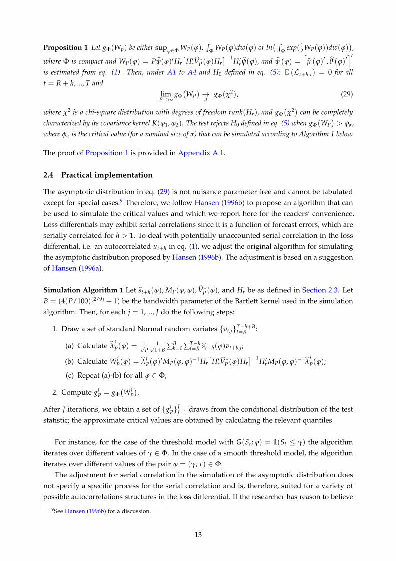
Figure 2 shows size-adjusted power for the three alternatives defined in equations (33) to(35). We compare the performance of our DMNL with that of Giacomini and White (2006) (GW,who formalized Diebold and Mariano, 1995) and the Giacomini and Rossi (2010) Fluctuation test.The solid lines with markers “+” and “o” display the ave-W results for the threshold model andlogistic smooth threshold model, and the dashed and dotted lines show the results for the GWand Fluctuation test, respectively.13 The three figures in Panel (a) show results for Alternative (1),i.e. state dependence without a constant deviation. As we can see, the size-adjusted power of ourDMNL increases quickly with the magnitude of the alternative as well as with the size of P. Sincethe DGP under the alternative is a threshold model, the LSTR exhibits rejection frequencies thatare smaller than those of the TR but nonetheless high. In turn, the GW and Fluctuation tests haveno power to detect the lack of equal predictive ability arising from the state dependence in therelative forecasting performance, and their power remains flat around the nominal size.14

The three figures in Panel (b) show results for Alternative (2), i.e. the case of a constant devia-

13Results for the exp-W and sup-W are virtually identical and available upon request.14Note that the Fluctuation test might have better power in cases where St is a persistent variable.

18

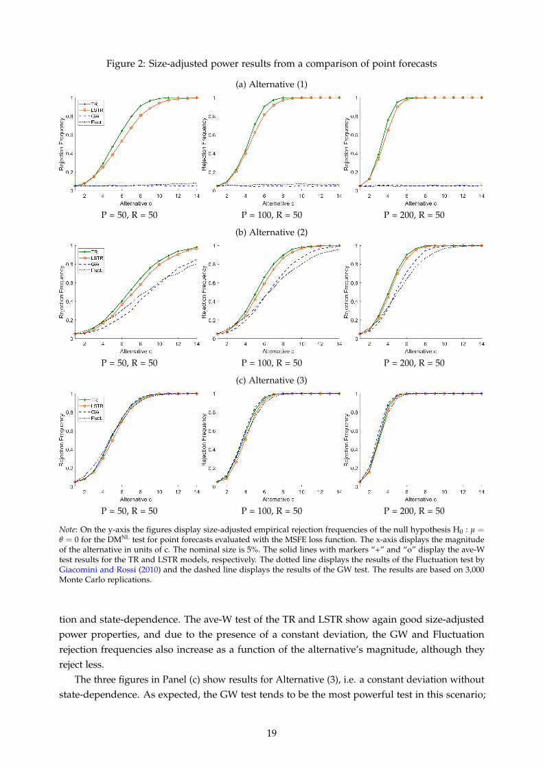
Figure 2: Size-adjusted power results from a comparison of point forecasts

P = 50, R = 50

(a) Alternative (1)

P = 100, R = 50 P = 200, R = 50

P = 50, R = 50

(b) Alternative (2)

P = 100, R = 50 P = 200, R = 50

P = 50, R = 50

(c) Alternative (3)

P = 100, R = 50 P = 200, R = 50

Note: On the y-axis the figures display size-adjusted empirical rejection frequencies of the null hypothesis H0 : µ =θ = 0 for the DMNL test for point forecasts evaluated with the MSFE loss function. The x-axis displays the magnitudeof the alternative in units of c. The nominal size is 5%. The solid lines with markers “+” and “o” display the ave-Wtest results for the TR and LSTR models, respectively. The dotted line displays the results of the Fluctuation test byGiacomini and Rossi (2010) and the dashed line displays the results of the GW test. The results are based on 3,000Monte Carlo replications.

tion and state-dependence. The ave-W test of the TR and LSTR show again good size-adjustedpower properties, and due to the presence of a constant deviation, the GW and Fluctuationrejection frequencies also increase as a function of the alternative’s magnitude, although theyreject less.

The three figures in Panel (c) show results for Alternative (3), i.e. a constant deviation withoutstate-dependence. As expected, the GW test tends to be the most powerful test in this scenario;

19

however, the power of the ave-W for both the TR and LSTR is very similar to that of the GW test.

3.3 Power for DGPs resulting in state-dependent forecast error losses

In the previous section, the alternative was modeled directly as a non-linear function of ∆Lt+1|t.In this section, we investigate power in two additional cases where the threshold behavior in theloss differential or the forecast encompassing loss is the result of non-linearities in the underlyingdata.

Common component DGP:In our first example, two observable variables, yt and xt, are driven by a common component, ct,and unpredictable idiosyncratic components, et and ut, respectively:

yt+1 = α + ct+1 + et+1, xt+1 = ct+1 + ηt+1, ct+1 = ρct + vt+1,

where α is a constant, et+1 ∼iid N(0, 1), ηt+1 ∼iid N(0, 1), and et+1, ηt+1, and vt+1 are mutuallyindependent. Importantly, vt+1 ∼ N(0, σ2

v,t+1), i.e. the variance is time-varying such that

σv,t+1 =

σv,L if St ≥ γ

σv,H if St < γ,

where σv,H > σv,L, i.e. the variance of the common component is a threshold-function of the stateSt. In other words, one can interpret xt as a proxy for the common cycle and St as a proxy for theunobserved strength of the common cycle.

In fact, in periods when St < γ, the shocks to the common component have a larger variancethen in periods when St ≥ γ, which increases the importance of the common cycle relative to theidiosyncratic error and, therefore, increases the comovement between xt and yt+1.15

The benchmark forecasting model is the simple historical average while the competitor modeluses xt as a predictor:

f (1)t+1|t =1R

t

∑i=t−R+1

yi and f (2)t+1|t = αt,R + βt,Rxt, (36)

where αt,R, βt,R are estimated by regressing yt+1 on a constant and xt, using a rolling windowestimation scheme of size R. These forecating models are similar to the ones that we consider inthe empirical analysis in Section 4.

Notice how the threshold in the volatility of the common component generates time-variationin the relative forecasting performance: when St ≥ γ, the comovement between yt+1 and xt isweaker such that xt is a very noisy predictor. However, when St < γ, the forecasting modelusing xt (the observable proxy of the common cycle) outperforms the historical mean predictionbecause the cyclical component dominates in these periods. Due to the autocorrelation in ct, thiseffect will last for some periods even after St falls below the threshold again.

For the Monte Carlo study, we set α = 0.5, ρ = 0.8, and σv,L = 0.1. The small valuefor σv,L implies that during calm periods, i.e. when St ≥ γ, the common component is of

15Lagged values of xt+1 are correlated with yt+1 due to the persistence in the cycle.

20

negligible importance for the forecasting performance; the idiosyncratic and unpredictable erroret dominates. In turn, all else equal, the comovement of yt+1 and xt increases in σv,H such that thecompetitor model’s relative performance in periods of St < γ also increases in σv,H. Therefore,to investigate the power of our methodology to detect periods of predictability, we let σv,H varyover a grid of equally spaced points in the interval [0.1, 1.6].16 The threshold variable we use isthe same as in our empirical application of Section 4, that is the monthly U.S. real GDP growthestimate of Koop et al. (2020), which ranges from 1960:M6 to 2020:M12 (see Section 4 for moredetails on the variable). We set the true threshold value in the simulations to γ = 1, and treat it asunknown in the estimation of the threshold model on the loss differential and encompassing loss.The in-sample estimation size is R = 240 (as in our empirical application in Section 4), whichleads to an out-of-sample size of P = 487.

Figure 3 displays the results. Panel (a) shows the power of the DMNL ave-W test for a thresholdregression model (TR, solid line with “+” markers) and a logistic smooth threshold regressionmodel (LSTR, solid line with “o” markers), as well as for the Giacomini and White (2006) (dashedline) and Fluctuation tests (dotted line). The x-axis displays the grid of values of σv,H and they-axis shows the rejection frequency at the 5% percent nominal level. We observe that ourproposed methodology has better power than the GW and Fluctuation tests as σv,H increases. Thisis because, for large values of σv,H, the relative performance of the competitor model improvesin periods when St < γ (the persistence in ct controls how the superior performance of thecompetitor model smoothes out over time). Therefore, in these periods, the mean squared forecasterror (MSFE) of the competitor model is lower than that of the historical average.

Panel (b) shows the power of the DMNL ave-W test for forecast encompassing, i.e. whether thefirst model encompasses the second model (again, the solid line with “+” markers denote the TRspecification and the solid line with “o” markers denote the LSTR specification), as well as ofthe Giacomini and White (2006) (dashed line) and Fluctuation tests (dotted line). Our proposedmethodology and Giacomini and White (2006) have very similar power.

Panel (c) shows one draw of the simulated loss differentials (solid line) alongside St (dashedline) and the value of γ = 1 (dotted line). When the dashed line is below the dotted horizontalline, we have that σv,t+1 = σv,H, i.e. the signal of the common component is relatively stronger.In turn, grey shaded areas indicate periods for which our threshold model, estimated on theloss differential, assigns a superior predictive ability to the competitor model. In other words,comparing periods where the dashed line is below the horizontal dotted line with the grey shadedareas provides a visual inspection of whether our modeling strategy of the loss differential canidentify actual periods of superior predictive ability in the simulated data. As the figure shows,the grey shaded areas coincide with periods where St < γ in the underlying DGP, indicating thatour methodology can recover such periods.

16Note that a null hypothesis of equal predictive ability or forecast encompassing does not hold for any of the valuesfor σv,H because even for σv,H = 0.1 the common component is present in the DGP although with very small signal tonoise ratio.

21

Figure 3: Common component DGP: power

(a) Equal predictive ability (b) Forecast encompassing

(c) Draw of simulated loss differential

Note: Panel (a) shows the power of the equal predictive ability test of the DMNL ave-W as well as of the Giacominiand White (2006) and Fluctuation tests. Panel (b) shows power for the forecast encompassing test of the DMNL ave-Was well as for the Giacomini and White (2006) and Fluctuation tests. The x-axis displays the grid of values of σv,Hand the y-axis shows rejection frequencies at a 5% percent nominal level. Panel (c) shows a draw of a simulated lossdifferential (solid line, positive numbers indicate a better forecast of the model using xt) alongside St (dashed line),and the value of γ = 1 (dotted line). Grey shaded areas indicate periods where our estimated threshold model assignsa superior predictive ability to the model that uses xt as a predictor.

22

Threshold regression DGP:In our second example, there is a threshold relationship present in the underlying data that isunknown to the forecaster and, therefore, not modeled in either of the competing predictionmodels. This translates into a threshold relationship in the loss differentials (encompassing loss).Specifically, the underlying data, yt, is generated by

yt+1 = α + ρyt + θ1zt,1 + θ2zt,2 + β · 1(St ≥ γ)xt + et+1, (37)

with et, zt,1, zt,2 ∼iid N(0, 1), xt = ρxxt−1 + ηt, with ηt ∼iid N(0, 2), and St and γ are the indicatorvariable and threshold value that we specify below. The variable xt is only present in the DGP inperiods for which St is bigger than the threshold γ.

We first consider the case where the two competing forecasting models used to computethe loss differential for conditional mean predictions, labeled benchmark and competitor modelrespectively, are non-nested17:

f (1)t+1|t = α1,t,R + ρ1,t,Ryt + θ1,t,Rzt,1 and f (2)t+1|t = α2,t,R + ρ2,t,Ryt + θ2,t,Rzt,2 + β2,t,Rxt, (38)

where α1,t,R, ρ1,t,R, and θ1,t,R are estimated by regressing yt on a constant, yt−1, and zt−1,1; andα2,t,R, ρ2,t,R, θ2,t,R, and β2,t,R are estimated by regressing yt on a constant, yt−1, zt−1,2, and xt−1.Note that the non-linear relationship β · 1(St ≥ γ)xt is unknown to the forecaster. All parametersare estimated using a rolling window of size R, given below.

For the forecast encompassing test, the two competing forecasting models are nested18, suchthat:

f (1)t+1|t = α1,t,R + ρ1,t,Ryt and f (2)t+1|t = α2,t,R + ρ2,t,Ryt + β2,t,Rxt, (39)

where the parameter are estimated as before but excluding zt−1,1 and zt−1,2, respectively, from theregressions.

Notice that the competitor model will outperform the benchmark model when St ≥ γ, since itincorporates information from xt into the forecast. However, the competitor model uses xt as apredictor independently of the value of St and, therefore, performs worse than the benchmarkwhen St < γ. The larger is β, all else equal, the more the relative performance of the twocompeting models differs in the two states St ≥ γ and St < γ. Therefore, in our Monte Carlostudy, we set α = ρ = ρx = θ1 = θ2 = 0.8, and let β vary over a grid of equally spaced pointsin the interval [0, 1.4]. For the threshold indicator variable St we use the adjusted NationalFinancial Conditions Index (ANFCI), computed by the Chicago Fed (see the empirical applicationin Section 5 for details), from 1971:M1 to 2019:M12. In the simulation of the DGP in eq. (37), weset the true threshold value γ to zero, and treat it as unknown when estimating the thresholdmodel on the loss differential and the encompassing loss. We set R = 120 (as in our empiricalapplication in Section 5) for the in-sample estimation window size of the models in eq. (38) and(39), which results in P = 480 given the ANFCI sample.

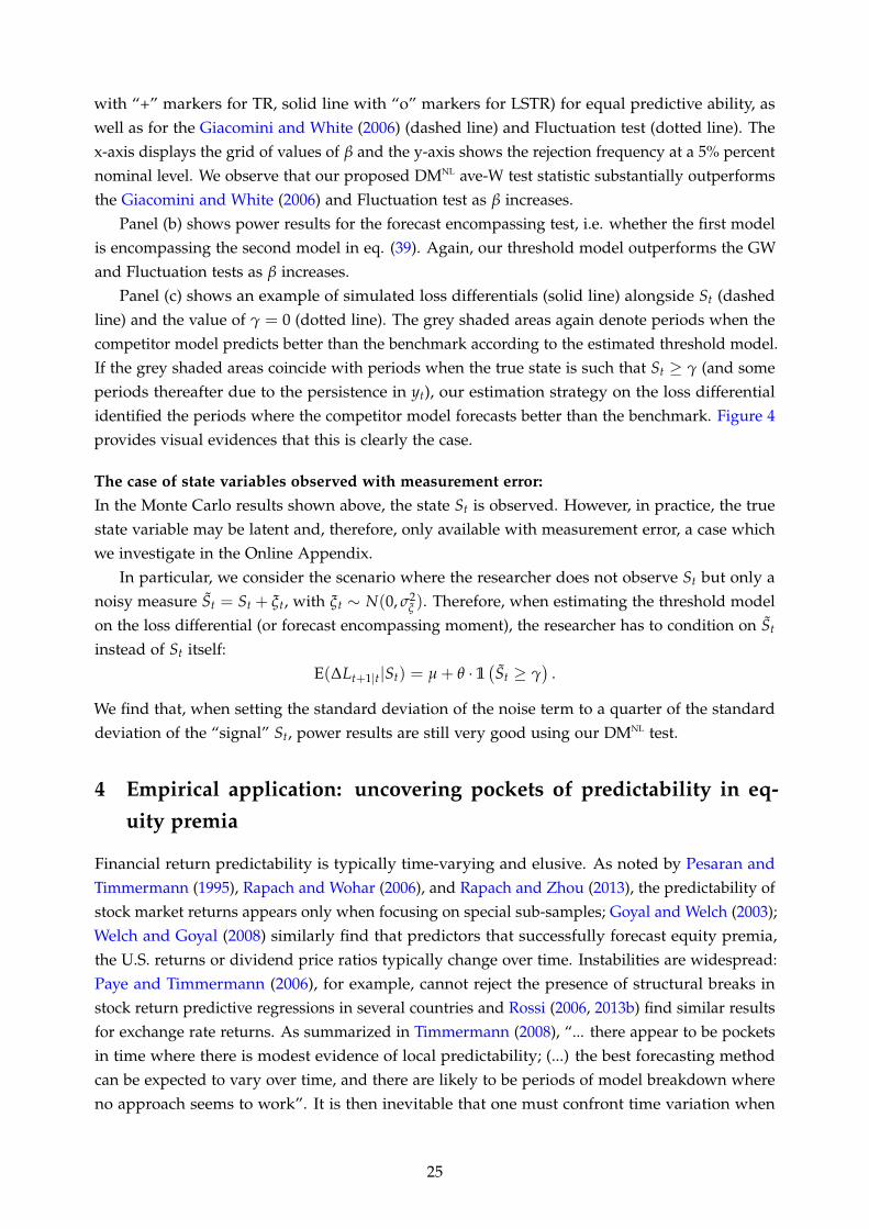
Figure 4 displays the results. Panel (a) shows the power of the DMNL ave-W test (solid line

17Since the common component DGP’s forecasting models were nested and because it is known that GW performsbetter in finite sample when using non-nested models, we added the predictors zt,1 and zt,2.

18We dropped zt,1 and zt,2 from the predictions to avoid rejections of the null of “no forecast encompassing” due tozt,1 or zt,2.

23

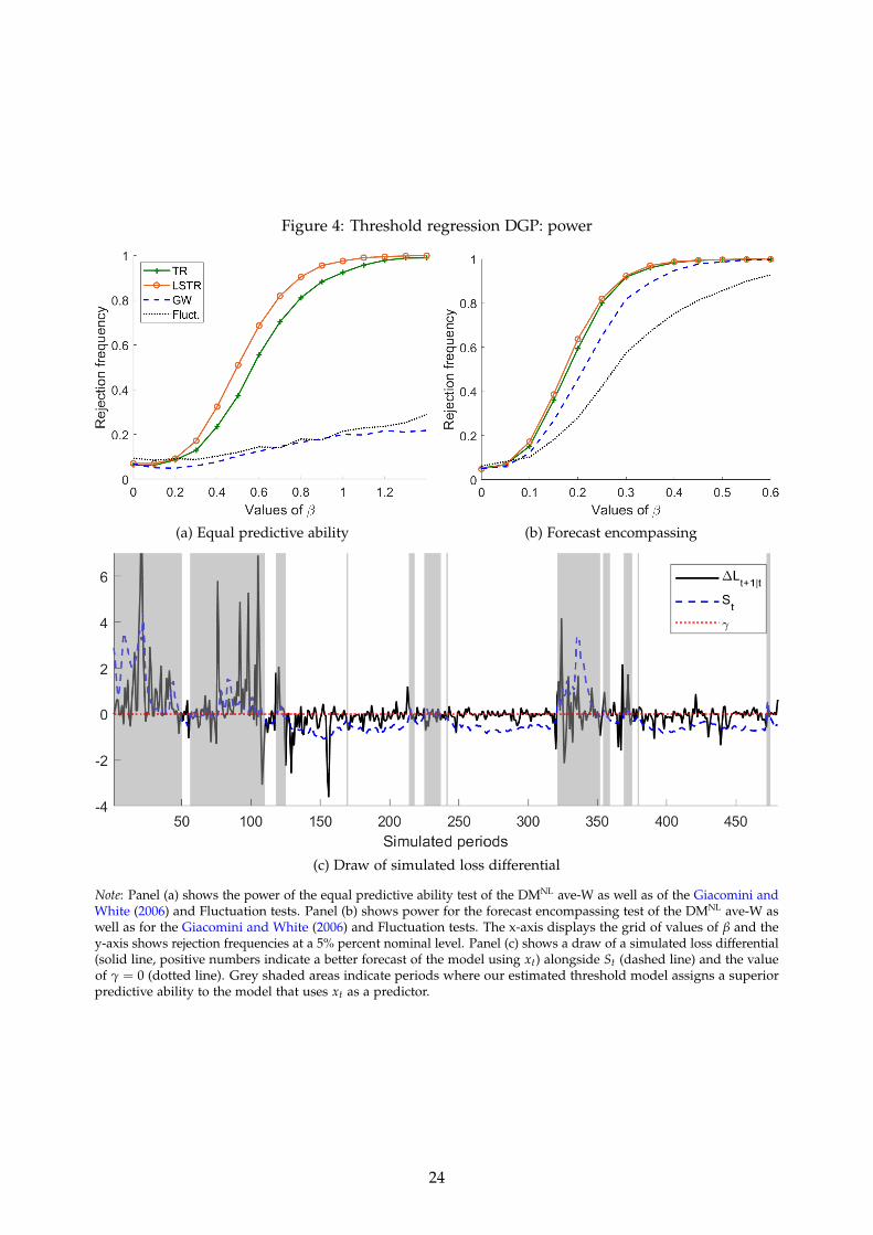
Figure 4: Threshold regression DGP: power

(a) Equal predictive ability (b) Forecast encompassing

(c) Draw of simulated loss differential

Note: Panel (a) shows the power of the equal predictive ability test of the DMNL ave-W as well as of the Giacomini andWhite (2006) and Fluctuation tests. Panel (b) shows power for the forecast encompassing test of the DMNL ave-W aswell as for the Giacomini and White (2006) and Fluctuation tests. The x-axis displays the grid of values of β and they-axis shows rejection frequencies at a 5% percent nominal level. Panel (c) shows a draw of a simulated loss differential(solid line, positive numbers indicate a better forecast of the model using xt) alongside St (dashed line) and the valueof γ = 0 (dotted line). Grey shaded areas indicate periods where our estimated threshold model assigns a superiorpredictive ability to the model that uses xt as a predictor.

24

with “+” markers for TR, solid line with “o” markers for LSTR) for equal predictive ability, aswell as for the Giacomini and White (2006) (dashed line) and Fluctuation test (dotted line). Thex-axis displays the grid of values of β and the y-axis shows the rejection frequency at a 5% percentnominal level. We observe that our proposed DMNL ave-W test statistic substantially outperformsthe Giacomini and White (2006) and Fluctuation test as β increases.

Panel (b) shows power results for the forecast encompassing test, i.e. whether the first modelis encompassing the second model in eq. (39). Again, our threshold model outperforms the GWand Fluctuation tests as β increases.

Panel (c) shows an example of simulated loss differentials (solid line) alongside St (dashedline) and the value of γ = 0 (dotted line). The grey shaded areas again denote periods when thecompetitor model predicts better than the benchmark according to the estimated threshold model.If the grey shaded areas coincide with periods when the true state is such that St ≥ γ (and someperiods thereafter due to the persistence in yt), our estimation strategy on the loss differentialidentified the periods where the competitor model forecasts better than the benchmark. Figure 4provides visual evidences that this is clearly the case.

The case of state variables observed with measurement error:In the Monte Carlo results shown above, the state St is observed. However, in practice, the truestate variable may be latent and, therefore, only available with measurement error, a case whichwe investigate in the Online Appendix.

In particular, we consider the scenario where the researcher does not observe St but only anoisy measure St = St + ξt, with ξt ∼ N(0, σ2

ξ ). Therefore, when estimating the threshold modelon the loss differential (or forecast encompassing moment), the researcher has to condition on St

instead of St itself:E(∆Lt+1|t|St) = µ + θ · 1

(St ≥ γ

).

We find that, when setting the standard deviation of the noise term to a quarter of the standarddeviation of the “signal” St, power results are still very good using our DMNL test.

4 Empirical application: uncovering pockets of predictability in eq-uity premia

Financial return predictability is typically time-varying and elusive. As noted by Pesaran andTimmermann (1995), Rapach and Wohar (2006), and Rapach and Zhou (2013), the predictability ofstock market returns appears only when focusing on special sub-samples; Goyal and Welch (2003);Welch and Goyal (2008) similarly find that predictors that successfully forecast equity premia,the U.S. returns or dividend price ratios typically change over time. Instabilities are widespread:Paye and Timmermann (2006), for example, cannot reject the presence of structural breaks instock return predictive regressions in several countries and Rossi (2006, 2013b) find similar resultsfor exchange rate returns. As summarized in Timmermann (2008), “... there appear to be pocketsin time where there is modest evidence of local predictability; (...) the best forecasting methodcan be expected to vary over time, and there are likely to be periods of model breakdown whereno approach seems to work”. It is then inevitable that one must confront time variation when

25

evaluating financial models’ predictive ability in an attempt to track their ”local” forecastingperformance.

As discussed in Timmermann (2008) and Paye and Timmermann (2006), the predictability ofequity premia could be caused by market inefficiencies. If that is the case, then rational investorswill take the opportunity to trade and make profits. However, if a large number of investorsengage in taking advantage of the predictability, their behavior will eventually eliminate thepredictability altogether. This implies the existence of short windows of time in which equitypremia are predictable, but a low (or no) predictability in the rest of the sample.

In what follows, we attempt to uncover pockets of predictability in U.S. equity premia inout-of-sample. We consider several of the classic economic predictors considered in Welch andGoyal (2008): the book to market ratio (calculated as the ratio of the book value and the marketvalue of the Dow Jones Industrial Average and labeled “BookToMarket”); the default yield spread(calculated as the difference between BAA and AAA-rated corporate bond yields and labeled“DFY”); a monthly inflation measure based on the Consumer Price Index (labeled “Inflation”); astock variance measure computed as the sum of squared daily returns (labeled “StockVar”); thelong-term government bond yield (labeled “LongYield”); the short-term government bond yield(labeled “Tbill”); and the term spread (calculated as the difference between the long-term yieldon government bonds and the Tbill and labeled "Spread").19

Then, the economic models are as follows:

Et−1rt = ν + δzt−1, (40)

where rt is the equity premium, zt−1 is the lagged economic predictor and ν is the intercept.As the benchmark model, we focus on the historical mean. All models are estimated using awindow of the past twenty years of data, i.e. R = 240, producing a series of rolling one-step-aheadout-of-sample forecasts.20

We estimate the ”local” forecasting performance using a non-linear model in the loss differ-ences, where the loss difference is the difference in the squared out-of-sample forecast error ofthe benchmark (historic rolling mean) minus that of the economic model (eq. 40):

E(∆Lt+1|t|St) = µ + θ · 1 (St ≥ γ) . (41)

Following the existing literature on the countercyclicality of equity premia, we use a measureof monthly real GDP growth, computed by Koop et al. (2020), as our indicator variable. Koopet al. (2020) impute a “true", yet unobserved, monthly real GDP growth series based on a mixed-frequency Bayesian Vector Autoregression (BVAR), using accounting identities as well as GDPexpenditure-side and GDP income-side estimates as observables. Their monthly GDP growthseries ranges from 1960:M6 to 2020:M12.21

We chose output growth as the state variable since stock returns are linked, by the net present

19The data are from A. Goyal’s website: http://www.hec.unil.ch/agoyal/.20Welch and Goyal (2008) use 20 years of monthly data and Harvey et al. (2021) use around 20 years of monthly

data for their results, both based on a rolling window estimation scheme. We provide robustness results for differentwindow sizes below.

21We are using the January 2021 vintage of Koop et al. (2020), who update the monthly real GDP growth serieswhen new data become available. In unreported results, we find that using other vintages available from Koop et al.(2020) leads to the same results as presented here.

26

value theory, to current and future output growth. Using a similar argument, Neely et al. (2014)and Henkel et al. (2011), for example, show that return predictability is linked to economicrecessions. In fact, equity premia are countercyclical (Campbell and Cochrane, 1999; Bekaertet al., 2009) and return predictability is correlated with the business cycle (Neely et al., 2014;Dangl and Halling, 2012; Henkel et al., 2011; Rapach et al., 2010). In particular, when predictingmonthly equity premia, Neely et al. (2014) find that economic predictors, especially the termspread and default yield spread, as well as technical indicators, beat the benchmark mean forecastduring NBER-dated recession periods. Relative to Neely et al. (2014) and Henkel et al. (2011), ouranalysis has the advantage that we can formalize the link between predictability and the businesscycle using a non-linear model for the forecast error loss.

The idea, formalized in eq. (41), is to capture Timmermann’s (2008) ”pockets of predictability”,where the pockets of predictability depend on the state of the business cycle. That is, the relativeperformance of the models changes over time depending on whether real GDP growth is higher(or lower) than an unknown threshold value. Note that a positive loss differential implies that theeconomic model is better than the benchmark (the historical mean).

In addition, we are interested in testing for forecast encompassing; in fact, it could be the casethat some of the predictors result in forecasts that are similar to the mean forecast in terms ofaccuracy but nonetheless have predictive power that is neglected by the benchmark model. Toassess whether the benchmark forecast encompasses the forecast using an economic predictor ina state-dependent manner, we estimate:

E(ε2t+1|t,1 − εt+1|t,1εt+1|t,2|St) = µ + θ · 1 (St ≥ γ) , (42)

where εt+1|t,1 denotes the forecast error of the mean model, and εt+1|t,2 denotes the forecast errorof the model with the economic predictor.

Table 2 reports the results of equal predictive ability (Panel A) and the forecast encompassingtests (Panel B). Since our forecasting exercise is most closely related to Neely et al. (2014), ourbaseline results use the same out-of-sample period as Neely et al. (2014), from 1966:M1 to2011:M12; results for alternative samples are similar and shown in the Online Appendix. For eachpredictor, listed in the first column, we report the p-values for the sup-W, ave-W, and exp-W test.In addition, we report the p-value of the Giacomini and White (2006) (GW) and the Fluctuationtests, and the out-of-sample size (for the Fluctuation we only indicate whether the p-value issmaller or larger than 0.10 or 0.05). For the case where the DMNL tests reject the null hypothesisof equal performance/forecast encompassing, we report the estimated parameters of the modeldefined in eq. (41) in Table 3. In addition, Table 3 reports the results of t-tests on the parameters,a Wald test on the sum of the parameters, the estimated threshold parameter, and the frequencyof the states.

Panel A of Table 2 shows that we find evidence of pockets of predictability when forecastingusing the term spread. The estimate of µ, shown in Table 3, is positive indicating that the lossdifference is positive when real GDP growth is lower than the threshold value, in which case theeconomic model has a better predictive ability than the benchmark model. However, when realGDP growth is high, the loss difference becomes negative. That is, the spread adds noise to theprediction of the returns during periods of at least moderate GDP growth, while the oppositeis true when GDP growth is low. Panel B of Table 2 shows that the results regarding the term

27

spread hold when testing for forecast encompassing as well.Notice that, unlike our proposed tests, the GW test does not find significant differences

between the model with the spread and the benchmark. This is because our test is more powerfulto detect pockets of predictability when there are instabilities associated with non-linearities.Notice that the Giacomini and Rossi (2010) Fluctuation test statistic is not bigger than the criticalvalue in the case of the spread either; hence, even though the Fluctuation test is robust toinstabilities in the relative forecasting performance, it is nevertheless less powerful than the testproposed in this paper and, in our data, never finds evidence of predictive ability, possibly due toits sporadic appearance over time.

Our results are related to previous work, for instance, Neely et al. (2014), who found evidencethat the term spread is capable of predicting equity premia during economic recessions. However,they differ in two important ways. Firstly, our paper is the first to use a monthly real GDP growthseries and formally test for non-linearity in the loss differentials; in fact, previous papers reliedon pre-defined NBER recession dummies or quarterly GDP data (Rapach et al., 2010). Secondly,using monthly real GDP growth in combination with our methodology, we find that the pockets ofpredictability are correlated with, but are not limited to, recessionary periods. In particular, thereare 148 months that our model identified as pockets of predictability but which are not classifiedas NBER recession dates. Our results, therefore, suggest that the pockets of predictability are notonly correlated with the business cycle but also present outside NBER recession dates.

Table 4 sheds further light on what drives the relative forecasting performance. It showsthe two competing forecasts’ MSFEs for different subsamples: the full out-of-sample as well asthe two subsamples identified by St ≥ γ and St < γ. In periods of high real GDP growth, i.e.when St ≥ γ, the performance improves for both forecasts relative to the full sample, but lessso for the forecast obtained with the spread as a predictor. In turn, during periods of low realGDP growth, i.e. when St < γ, both the simple mean as well as the forecast obtained with theeconomic predictor perform worse, but the latter less so.

We further conducted a number of robustness checks. In the first robustness check, weincreased (decreased) R, the in-sample estimation window size, to 300 (180) observations. Resultsare reported in Appendix C — in particular, see Table C.1, for the test of equal predictive ability,and Table C.2, for the forecast encompassing test. The results are similar even with differentin-sample estimation window sizes.

In the second robustness check, reported in Table C.3, we add monthly real GDP growth as alinear control variable in eq. (41), i.e. E(∆Lt+1|t|St) = µ + θ · 1 (St ≥ γ) + φSt, and test µ = θ = 0.As in the baseline result in Table 2, our test rejects the null hypothesis for the spread, pointing outthat a simple linear conditional test would not be sufficient to uncover the non-linear relationshipbetween GDP growth and the pockets of predictability.

In the third robustness exercise, reported in the Online Appendix, we show that our resultsare robust to specifying the out-of-sample period as 1966:M1 to 2006:M12 (pre-financial crisis),1966:M1 to 2017:M12 (the end of the Welch and Goyal, 2008 dataset), or 1960:M6 (the start of themonthly GDP series) to 2011:M12.

For the spread, for which we found that the economic model performs sometimes better thanthe benchmark, Figure 5 reports the loss differences (∆Lt+1|t, solid line) over time, together withthe monthly real GDP growth series (St, dashed line) that triggers the state-switching. Shaded

28

areas depict periods where the economic model has, on average, a lower squared forecast errorthan the benchmark model (the loss difference is positive on average). Periods that are not shadedindicate times in which the benchmark model performs better than the economic model. Thefigure shows that there are several pockets of predictability, where the economic model predictsslightly better than the benchmark. Furthermore, these pockets persist for a few periods and areinterrupted by periods when the economic model performs worse than the benchmark, causingthe average performance of the model to be poor over the entire sample.

Farmer et al. (2019) also find evidence in favor of pockets of in-sample predictability in U.S.equity premia using the term spread. Their methodology is very different from ours, as theyemploy a time-varying parameter model estimated non-parametrically while we model directlythe forecast loss differential. In addition, they focus on equity premia at a daily frequency, whilewe have data at a monthly frequency. Despite these differences, several of their identified pocketsare similar to ours.

In particular, our pockets identified for the beginning of the 1970s, the mid-1970s, and thebeginning of the 1980s coincide with the in-sample findings of Farmer et al. (2019) for the termspread. Moreover, Farmer et al. (2019) show out-of-sample results for daily data using a bivariatemodel with the term spread and the Tbill as predictors. Again, the pockets they find at thebeginning of the 1970s, the mid-1970s, and the beginning of the 1980s coincide with ours for theterm spread.

Table 2: State-dependence in equity premium forecasts

Variable Name DMNL Alternative statistics Sample size

Panel A. Loss differentialsup-W ave-W exp-W GW Fluct. P

DFY 0.144 0.278 0.242 0.523 < 0.10 552Inflation 0.586 0.538 0.539 0.602 > 0.10 552StockVar 0.515 0.463 0.469 0.238 > 0.10 552LongYield 0.855 0.729 0.743 0.700 > 0.10 552Spread 0.020 0.031 0.020 0.570 > 0.10 552Tbill 0.774 0.724 0.734 0.896 > 0.10 552BookToMkt 0.408 0.156 0.194 0.070 < 0.10 552

Panel B. Forecast encompassingsup-W ave-W exp-W GW Fluct. P

DFY 0.453 0.458 0.465 0.416 > 0.10 552Inflation 0.034 0.021 0.024 0.054 < 0.05 552StockVar 0.576 0.566 0.575 0.504 > 0.10 552LongYield 0.768 0.449 0.507 0.260 > 0.10 552Spread 0.002 0.001 0.001 0.002 < 0.05 552Tbill 0.396 0.129 0.165 0.073 > 0.10 552BookToMkt 0.460 0.270 0.307 0.163 > 0.10 552

Note: The table shows p-values of tests of equal predictive ability (Panel A) and forecast encompassing(Panel B) using the DMNL, the GW, and the Fluctuation test (for the Fluctuation test we only indicatewhether the p-value is smaller or larger than 0.10 or 0.05). Boldface numbers indicate significance at the10% level. The in-sample estimation window size, R, is 240.

29

Figure 5: Pockets of predictability using the term spread

Note: The figure shows the estimated ∆Lt+1|t (solid line, positive numbers indicate that the economic model forecastsbetter than the mean model) together with the monthly real GDP growth measure St (dashed line), which triggersthe state-switching, for the term spread as the predictor. Shaded areas indicate periods where the economic modelperforms better than the benchmark, i.e. they show the pockets of predictability.

Table 3: State-dependent estimates: eq. (41) and (42)

Predictor Parameter estimates Parameter tests State characteristicsµ θ µ + θ γ µ = 0 θ = 0 µ + θ = 0 S P(St ≥ γ)

Panel A. Loss differentialSpread 0.190 −0.284 −0.093 0.779 3.793 −3.248 1.554 0.922 0.592

Panel B. Forecast encompassingSpread 0.288 −0.274 0.014 0.779 6.113 −2.819 0.027 0.922 0.592Inflation −0.006 0.092 0.086 0.086 −0.221 0.501 0.223 0.922 0.842

Note: The table shows the parameter estimates associated with the equation in (41) and (42). The columns µ, θ, µ + θ, andγ show the parameter estimates associated with the sup-W statistic. The columns µ = 0, θ = 0, and µ + θ = 0 show thevalues of the statistic when using a t-test or a Wald test respectively, for testing the hypothesis that the parameters, or theirsum, are equal to zero. The critical values of a Wald test, with one restriction, at the 5% and 10% level are 2.706 and 3.842.Boldface numbers indicate a rejection at the 10% level. The column S shows the average value of the conditioning variableSt, and P(St ≥ γ) shows the relative frequency of being in the state where both µ and θ are present.

Finally, note that, in this paper, we focus on detecting “pockets of predictability” in historicaldata and linking it to the time-variation in an economic threshold variable. For readers interestedin methodologies specifically tailored for real-time detection, Inoue and Rossi (2015) and Harveyet al. (2021) propose monitoring procedures to detect structural changes. They suggest sequentiallyrepeating t-tests over short time periods and control the overall rejection rates. For example, intheir application to predictive regressions, Harvey et al. (2021) find that the one-month ahead

30

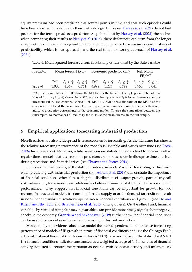
equity premium had been predictable at several points in time and that such episodes couldhave been detected in real-time by their methodology. Unlike us, Harvey et al. (2021) do not findpockets for the term spread as a predictor. As pointed out by Harvey et al. (2021) themselveswhen comparing their results to Neely et al. (2014), these differences can stem from the longersample of the data we are using and the fundamental difference between an ex-post analysis ofpredictability, which is our approach, and the real-time monitoring approach of Harvey et al.(2021).

Table 4: Mean squared forecast errors in subsamples identified by the state variable

Predictor Mean forecast (MF) Economic predictor (EP) Rel. MSFE:EP/MF

Full St < γ St ≥ γ Full St < γ St ≥ γ St < γ St ≥ γSpread 1.000 1.347 0.761 0.992 1.283 0.792 0.952 1.041

Note: The column labeled “Full” shows the MSFEs over the full out-of-sample period. The columnlabeled St < γ (St ≥ γ) shows the MSFE in the subsample where St is lower (greater) than thethreshold value. The columns labeled “Rel. MSFE: EP/MF” show the ratio of the MSFE of theeconomic model and the mean model in the respective subsamples; a number smaller than oneindicates a superior performance of the economic model. To ease the comparison between thesubsamples, we normalized all values by the MSFE of the mean forecast in the full sample.

5 Empirical application: forecasting industrial production

Non-linearities are also widespread in macroeconomic forecasting. As the literature has shown,the relative forecasting performance of the models is unstable and varies over time (see Rossi,2013a for a reference). Moreover, while parsimonious statistical models tend to forecast well inregular times, models that use economic predictors are more accurate in disruptive times, such asduring recessions and financial crises (see Chauvet and Potter, 2013).

In this section, we investigate the state dependence in models’ relative forecasting performancewhen predicting U.S. industrial production (IP). Adrian et al. (2019) demonstrate the importanceof financial conditions when forecasting the distribution of output growth, particularly tailrisk, advocating for a non-linear relationship between financial stability and macroeconomicperformance. They suggest that financial conditions can be important for growth for tworeasons. In structural models, frictions in either the supply of or the demand for credit can resultin non-linear equilibrium relationships between financial conditions and growth (see He andKrishnamurthy, 2011 and Brunnermeier et al., 2013, among others). On the other hand, financialvariables, by virtue of being fast-moving variables, can provide more timely signals about negativeshocks to the economy. Granziera and Sekhposyan (2019) further show that financial conditionscan be useful for model selection when forecasting industrial production.

Motivated by the evidence above, we model the state-dependence in the relative forecastingperformance of models of IP growth in terms of financial conditions and use the Chicago Fed’sadjusted National Financial Conditions Index (ANFCI) as an indicator for the state. The ANFCIis a financial conditions indicator constructed as a weighted average of 105 measures of financialactivity, adjusted to remove the variation associated with economic activity and inflation. By

31

construction, values above zero indicate financial conditions that are tighter than average. Weobtained the series from the database FRED of the Federal Reserve Bank of St. Louis. The relativeforecasting performance, however, could vary over time not only when the ANFCI is greaterthan zero, but also when it is above/below some other threshold value. We let the threshold beunknown and estimate it using our procedure. Our proposed tests detect the thresholds in themodels’ relative forecasting performance across financial cycles.

The forecasting environment is similar to Granziera and Sekhposyan (2019). The benchmarkis an autoregressive model of order p (AR(p)):

yt+1 = α + ρ(L)yt + et,

where yt is industrial production growth, ρ(L) = ρ + ρ1L + ... + ρpLp is a lag-polynomial with alag length of p, chosen by the BIC, which is re-estimated at each point in time. The competitor isan autoregressive-distributed lag model (ADL(p,q)) using one economic predictor at-a-time:

yt+1 = α + ρ(L)yt + φ(L)xt + et,

where φ(L) = φ + φ1L + ... + φqLq. The lag length p of the autoregressive component is givenfrom the AR(p), and we (re-)estimate q via the BIC, again, at each point in time.

We consider four macroeconomic variables and four financial variables as predictors (labeland FRED mnemonics are reported in parentheses): new privately-owned housing units started(labeled “Housing Starts," HOUST), the non-farm vacancies divided by the number of unemployed(labeled “VacancyToUr", HelpHWIURATIO), the employment level (labeled “Employment",CE16OV), new orders of durable goods (labeled “New Orders”, AMDMNOx), outstandingconsumer credit, measured by outstanding total nonrevolving credit owned and securitized(labeled “Consumer Credit”, NONREVSL), the spread between the one-year Treasury rate minusthe Federal Funds rate (FFR) (labeled “One Year Spread”, T1YFFM), the spread between theten-year Treasury rate and the FFR (labeled “Ten Year Spread”, T10YFFM), and the Moody’s BaaCorporate Bond rate minus the FFR (labeled “Credit Spread”, BAAFFM). These indicators arebroadly considered to be leading indicators for real economic activity. The data are from theFRED-MD database of McCracken and Ng (2016) and ranges from January 1959 to December2019. We transform the data as recommended in McCracken and Ng (2016) to ensure stationarity.

The forecasting horizon we consider is one month. The parameters α, ρ(L), and φ(L) areestimated using a rolling window of 10 years, i.e. 120 observations. Given the one-step-aheadforecasts of the AR(p) and ADL(p,q), we compute the loss differential, ∆Lt+1|t, as the differencebetween the squared forecast error of the AR(p) and the squared forecast error of the ADL(p,q).Then, we model the loss differential as

E(∆Lt+1|t|St) = µ + θ · 1 (St ≥ γ) , (43)

and we test the null hypothesis H0 : µ = θ = 0. Since the ANFCI series starts in 1971:M1, ourout-of-sample size is 587 observations.

Table 5 shows results for our test statistics. When we use the VacancyToUR, New Orders, andConsumer Credit as predictors, our sup-W, ave-W, and exp-W reject the null hypothesis of equal

32

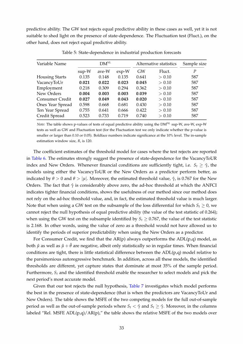
predictive ability. The GW test rejects equal predictive ability in these cases as well, yet it is notsuitable to shed light on the presence of state-dependence. The Fluctuation test (Fluct.), on theother hand, does not reject equal predictive ability.

Table 5: State-dependence in industrial production forecasts

Variable Name DMNL Alternative statistics Sample size

sup-W ave-W exp-W GW Fluct. PHousing Starts 0.135 0.148 0.135 0.641 > 0.10 587VacancyToUr 0.021 0.022 0.023 0.045 > 0.10 587Employment 0.218 0.309 0.294 0.362 > 0.10 587New Orders 0.004 0.003 0.003 0.039 > 0.10 587Consumer Credit 0.027 0.049 0.043 0.020 > 0.10 587Ones Year Spread 0.598 0.668 0.681 0.430 > 0.10 587Ten Year Spread 0.755 0.641 0.666 0.422 > 0.10 587Credit Spread 0.523 0.733 0.719 0.740 > 0.10 587

Note: The table shows p-values of tests of equal predictive ability using the DMNL sup-W, ave-W, exp-Wtests as well as GW and Fluctuation test (for the Fluctuation test we only indicate whether the p-value issmaller or larger than 0.10 or 0.05). Boldface numbers indicate significance at the 10% level. The in-sampleestimation window size, R, is 120.

The coefficient estimates of the threshold model for cases where the test rejects are reportedin Table 6. The estimates strongly suggest the presence of state-dependence for the VacancyToURindex and New Orders. Whenever financial conditions are sufficiently tight, i.e. St ≥ γ, themodels using either the VacancyToUR or the New Orders as a predictor perform better, asindicated by θ > 0 and θ > |µ|. Moreover, the estimated threshold value, γ, is 0.767 for the NewOrders. The fact that γ is considerably above zero, the ad-hoc threshold at which the ANFCIindicates tighter financial conditions, shows the usefulness of our method since our method doesnot rely on the ad-hoc threshold value, and, in fact, the estimated threshold value is much larger.Note that when using a GW test on the subsample of the loss differential for which St ≥ 0, wecannot reject the null hypothesis of equal predictive ability (the value of the test statistic of 0.264);when using the GW test on the subsample identified by St ≥ 0.767, the value of the test statisticis 2.168. In other words, using the value of zero as a threshold would not have allowed us toidentify the periods of superior predictability when using the New Orders as a predictor.

For Consumer Credit, we find that the AR(p) always outperforms the ADL(p,q) model, asboth µ as well as µ + θ are negative, albeit only statistically so in regular times. When financialconditions are tight, there is little statistical difference between the ADL(p,q) model relative tothe parsimonious autoregressive benchmark. In addition, across all these models, the identifiedthresholds are different, yet capture states that dominate at most 35% of the sample period.Furthermore, St and the identified threshold enable the researcher to select models and pick thenext period’s most accurate model.

Given that our test rejects the null hypothesis, Table 7 investigates which model performsthe best in the presence of state-dependence (that is when the predictors are VacancyToUr andNew Orders). The table shows the MSFE of the two competing models for the full out-of-sampleperiod as well as the out-of-sample periods where St < γ and St ≥ γ. Moreover, in the columnslabeled “Rel. MSFE ADL(p,q)/AR(p),” the table shows the relative MSFE of the two models over

33

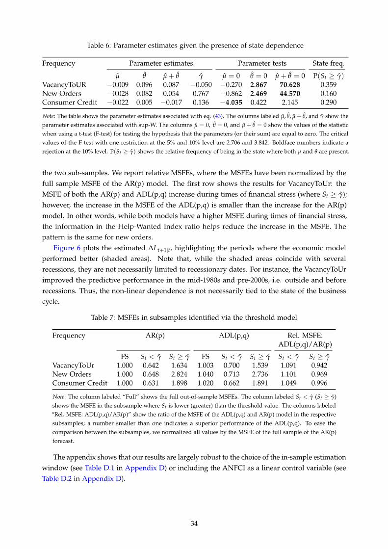
Table 6: Parameter estimates given the presence of state dependence

Frequency Parameter estimates Parameter tests State freq.

µ θ µ + θ γ µ = 0 θ = 0 µ + θ = 0 P(St ≥ γ)VacancyToUR −0.009 0.096 0.087 −0.050 −0.270 2.867 70.628 0.359New Orders −0.028 0.082 0.054 0.767 −0.862 2.469 44.570 0.160Consumer Credit −0.022 0.005 −0.017 0.136 −4.035 0.422 2.145 0.290

Note: The table shows the parameter estimates associated with eq. (43). The columns labeled µ, θ, µ + θ, and γ show theparameter estimates associated with sup-W. The columns µ = 0, θ = 0, and µ + θ = 0 show the values of the statisticwhen using a t-test (F-test) for testing the hypothesis that the parameters (or their sum) are equal to zero. The criticalvalues of the F-test with one restriction at the 5% and 10% level are 2.706 and 3.842. Boldface numbers indicate arejection at the 10% level. P(St ≥ γ) shows the relative frequency of being in the state where both µ and θ are present.

the two sub-samples. We report relative MSFEs, where the MSFEs have been normalized by thefull sample MSFE of the AR(p) model. The first row shows the results for VacancyToUr: theMSFE of both the AR(p) and ADL(p,q) increase during times of financial stress (where St ≥ γ);however, the increase in the MSFE of the ADL(p,q) is smaller than the increase for the AR(p)model. In other words, while both models have a higher MSFE during times of financial stress,the information in the Help-Wanted Index ratio helps reduce the increase in the MSFE. Thepattern is the same for new orders.

Figure 6 plots the estimated ∆Lt+1|t, highlighting the periods where the economic modelperformed better (shaded areas). Note that, while the shaded areas coincide with severalrecessions, they are not necessarily limited to recessionary dates. For instance, the VacancyToUrimproved the predictive performance in the mid-1980s and pre-2000s, i.e. outside and beforerecessions. Thus, the non-linear dependence is not necessarily tied to the state of the businesscycle.

Table 7: MSFEs in subsamples identified via the threshold model

Frequency AR(p) ADL(p,q) Rel. MSFE:ADL(p,q)/AR(p)

FS St < γ St ≥ γ FS St < γ St ≥ γ St < γ St ≥ γVacancyToUr 1.000 0.642 1.634 1.003 0.700 1.539 1.091 0.942New Orders 1.000 0.648 2.824 1.040 0.713 2.736 1.101 0.969Consumer Credit 1.000 0.631 1.898 1.020 0.662 1.891 1.049 0.996

Note: The column labeled “Full” shows the full out-of-sample MSFEs. The column labeled St < γ (St ≥ γ)shows the MSFE in the subsample where St is lower (greater) than the threshold value. The columns labeled“Rel. MSFE: ADL(p,q)/AR(p)” show the ratio of the MSFE of the ADL(p,q) and AR(p) model in the respectivesubsamples; a number smaller than one indicates a superior performance of the ADL(p,q). To ease thecomparison between the subsamples, we normalized all values by the MSFE of the full sample of the AR(p)forecast.

The appendix shows that our results are largely robust to the choice of the in-sample estimationwindow (see Table D.1 in Appendix D) or including the ANFCI as a linear control variable (seeTable D.2 in Appendix D).

34

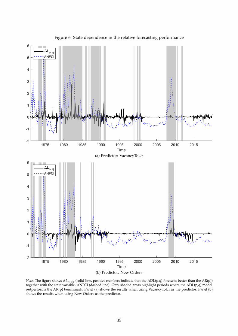
Figure 6: State dependence in the relative forecasting performance

(a) Predictor: VacancyToUr

(b) Predictor: New Orders

Note: The figure shows ∆Lt+1|t (solid line, positive numbers indicate that the ADL(p,q) forecasts better than the AR(p))together with the state variable, ANFCI (dashed line). Grey shaded areas highlight periods where the ADL(p,q) modeloutperforms the AR(p) benchmark. Panel (a) shows the results when using VacancyToUr as the predictor. Panel (b)shows the results when using New Orders as the predictor.

35

6 Conclusion

We have developed methodologies that allow researchers to test for the presence of non-linearitiesin the relative and absolute forecast error losses. Non-linear changes in the forecasting per-formance could be, for example, naturally generated in the presence of models with omittednon-linearities. For example, if the true data generating process is a threshold model, the forecasterror loss of a model with constant parameters may feature non-linear, threshold-type time-variation. Hence, our paper is useful in situations where the researcher expects the forecastperformance to be state-dependent. Currently, the only approach available to researchers isGiacomini and Rossi (2010), and, as we show, it is not the best approach to handle non-linearforecast error losses when the non-linearity is a function of an observable variable.

Our testing framework assumes that the parameters of the forecasting models are estimatedusing a rolling window scheme, i.e. we evaluate forecasting methods rather than forecastingmodels, and we allow for nested and non-nested models. Results from a Monte Carlo studyindicate good size and power properties of the test statistics for moderate and large sample sizes.

In the first empirical application, we document the existence of state dependence in the relativeforecasting performance when predicting stock returns. In particular, a model that only uses thehistorical mean as a predictor performs better during times of high real GDP growth, whereasa model that uses the term spread as a predictor has a better forecasting performance duringtimes of low real GDP growth. Hence, our results link predictability in returns to current outputgrowth. Existing tests, such as the Giacomini and White (2006) and Giacomini and Rossi (2010)tests, cannot detect these “pockets of predictability” as they lack power against state-dependence.

Since non-linearities are also widespread in macroeconomic forecasting, in the second empiri-cal application we investigate the relative forecasting performance of an autoregressive versus anautoregressive-distributed lag model for forecasting U.S. industrial production. The choice ofour state variable, the adjusted National Financial Conditions Index, is motivated by Adrian et al.(2019) who demonstrated the importance of financial conditions for forecasting the distributionof output growth, particularly tail risk, advocating for a non-linear relationship between financialstability and macroeconomic performance. Our proposed test detects state-dependence in theloss differentials of several predictors, indicating that the additional predictors used by theautoregressive-distributed lag model help forecasting U.S. industrial production during times oftight financial conditions.

36

References

Adrian, T., Boyarchenko, N., and Giannone, D. (2019). Vulnerable growth. American EconomicReview, 109(4):1263–89.

Amisano, G. and Giacomini, R. (2007). Comparing density forecasts via weighted likelihood ratiotests. Journal of Business & Economic Statistics, 25:177–190.

Andrews, D. and Ploberger, W. (1994). Optimal tests when a nuisance parameter is present onlyunder the alternative. Econometrica, 62:1383–1414.

Andrews, D. W. K. (1991). An empirical process central limit theorem for dependent nonidenticallydistributed random variables. Journal of Multivariate Analysis, 38:188–203.

Andrews, D. W. K. (1993). An introduction to econometric applications of empirical processtheory for dependent random variables. Econometric Reviews, 12:183–216.

Bekaert, G., Engstrom, E., and Xing, Y. (2009). Risk, uncertainty, and asset prices. Journal ofFinancial Economics, 91:59–82.

Brunnermeier, M. K., Eisenbach, T. M., and Sannikov, Y. (2013). Macroeconomics with financialfrictions: A survey, volume 2 of Econometric Society Monographs, page 3–94. Cambridge UniversityPress.

Campbell, J. Y. and Cochrane, J. (1999). Force of habit: a consumption-based explanation ofaggregate stock market behavior. Journal of Political Economy, 107:205–251.

Carrasco, M., Hu, L., and Ploberger, W. (2014). Optimal test for Markov switching parameters.Econometrica, 82:765–784.

Chauvet, M. and Potter, S. (2013). Forecasting output. In Elliot, G. and Timmermann, A., editors,Handbook of Economic Forecasting, volume 2, chapter 3, pages 141–194. Elsevier Publications.

Cho, J. S. and White, H. (2007). Testing for regime switching. Econometrica, 75:1671–1720.

Clark, T. and McCracken, M. (2001). Tests of equal forecast accuracy and encompassing for nestedmodels. Journal of Econometrics, 105:85–110.

Clark, T. and West, K. (2006). Using out-of-sample mean squared prediction errors to test themartingale difference hypothesis. Journal of Econometrics, 135:155–186.

Clark, T. and West, K. (2007). Approximately normal tests for equal predictive accuracy in nestedmodels. Journal of Econometrics, 138:291–311.

Dangl, T. and Halling, M. (2012). Predictive regressions with time-varying coefficients. Journal ofFinancial Economics, 106:157–181.

Davies, R. B. (1977). Hypothesis testing when a nuisance parameter is present only under thealternative. Biometrika, 64:247–254.

Davies, R. B. (1987). Hypothesis testing when a nuisance parameter is present only under thealternative. Biometrika, 74:33–43.

37

Diebold, F. X. and Mariano, R. S. (1995). Comparing predictive accuracy. Journal of Business &Economic Statistics, 13:253–263.

Dotsey, M., Fujita, S., and Stark, T. (2018). Do phillips curves conditionally help to forecastinflation. International Journal of Central Banking, 14:43–92.

Doukhan, P., Massart, P., and Rio, E. (1995). Invariance principles for absolutely regular empiricalprocesses. Annales de l’Institut H. Poincaré, 31:393–427.

Farmer, L., Schmidt, L., and Timmermann, A. (2019). Pockets of predictability. mimeo.

Garcia, R. (1998). Asymptotic null distribution of the likelihood ratio test in Markov switchingmodels. International Economic Review, 39:763–788.

Giacomini, R. and Rossi, B. (2010). Forecast comparisons in unstable environments. Journal ofApplied Econometrics, 25:595–620.

Giacomini, R. and White, H. (2006). Tests of conditional predictive ability. Econometrica, 74:1545–1578.

Goyal, A. and Welch, I. (2003). Predicting the equity premium with dividend ratios. ManagementScience, 49:639–654.

Granziera, E. and Sekhposyan, T. (2019). Predicting relative forecasting performance: an empiricalinvestigation. International Journal of Forecasting, 35:1636–1657.

Hamilton, J. D. (1989). A new approach to the economic analysis of non-stationary time seriesand the business cycle. Econometrica, 57:357–384.

Hansen, B. E. (1992). The likelihood ratio test under non-standard conditions: Testing the Markovswitching model of GNP. Journal of Applied Econometric, 7:61–82.

Hansen, B. E. (1996a). Erratum: The likelihood ratio test under non-standard conditions: Testingthe Markov switching model of GNP. Journal of Applied Econometrics, 11:195–198.

Hansen, B. E. (1996b). Inference when a nuisance parameter is not identified under the nullhypothesis. Econometrica, 64:413–430.

Hansen, B. E. (1996c). Stochastic equicontinuity for unbounded dependent heterogeneous arrays.Econometric Theory, 12:347–359.

Harvey, D., Leybourne, S. J., Sollis, R., and Taylor, A. M. R. (2021). Real-time detection of regimesof predictability in the US equity premium. Journal of Applied Econometrics, 36:45–70.

He, Z. and Krishnamurthy, A. (2011). A model of capital and crises. The Review of Economic Studies,79(2):735–777.

Henkel, S. J., Martin, J. S., and Nardari, F. (2011). Time-varying short-horizon predictability.Journal of Financial Economics, 99:560–580.

Inoue, A. and Rossi, B. (2015). Recursive predictability tests for real time data. Journal of Business& Economic Statistics, 23:336–345.

38

Koop, G., McIntyre, S., Mitchell, J., and Poon, A. (2020). Reconciled estimates of monthly GDP inthe US. EMF Research Papers, Economic Modelling and Forecasting Group.

Liew, J. and Vassalou, M. (2000). Can book-to-market, size, and momentum be risk factors thatexplain economic growth. Journal of Financial Economics, 57:221–245.

McCracken, M. W. (2019). Tests of conditional predictive ability: Some simulation evidence.Working Paper Nr. 011C, Federal Reserve Bank of St. Louis.

McCracken, M. W. and Ng, S. (2016). FRED-MD: A monthly database for macroeconomic research.Journal of Business & Economic Statistics, 34:574–589.

Moench, E. and Stein, T. (2021). Equity premium predictability over the business cycle. Centre forEconomic Policy Research.

Neely, J. N., Rapach, D. E., Tu, J., and Zhou, G. (2014). Forecasting the equity risk premium: Therole of technical indicators. Management Science, 60:1772–1791.

Paye, B. and Timmermann, A. (2006). Instability of return prediction models. Journal of EmpiricalFinance, 13:274–315.

Pesaran, M. H. and Timmermann, A. (1995). Predictability of stock returns: Robustness andeconomic significance. Journal of Finance, 50:1201–1228.

Qu, Z. and Zhuo, F. (2020). Likelihood Ratio-Based Tests for Markov Regime Switching. TheReview of Economic Studies, 88(2):937–968.

Rapach, D., Strauss, J., and Zhou, G. (2010). Out-of-sample equity premium prediction: Combina-tion forecasts and links to the real economy. Review of Financial Studies, 23:821–862.

Rapach, D. and Wohar, M. (2006). Structural breaks and predictive regression models of aggregateU.S. stock returns. Journal of Financial Econometrics, 4:238–274.

Rapach, D. and Zhou, G. (2013). Forecasting stock returns. In Elliott, G., Granger, C., andTimmermann, A., editors, Handbook of Economic Forecasting, volume 2, pages 328–383. Elsevier.

Rossi, B. (2006). Are exchange rates really random walks? Some evidence robust to parameterinstability. Macroeconomic Dynamics, 10:20–38.

Rossi, B. (2013a). Advances in Forecasting under Model Instability. In Elliot, G. and Tmmermann,A., editors, Handbook of Economic Forecasting, volume 2, chapter 21, pages 1203–1324. ElsevierPublications.

Rossi, B. (2013b). Are exchange rates predictable? Journal of Economic Literature, 51:1063–1119.

Stock, J. H. and Watson, M. W. (2009). Phillips curve inflation forecasts. In Fuhrer, J., Kodrzycki,Y. K., Sneddon Little, J., and Olivei, G. P., editors, Understanding Inflation and the Implications forMonetary Policy: A Phillips Curve Retrospective. MIT Press.

Teräsvirta, T. (2006). Forecasting economic variables with nonlinear models. In Elliott, G., C. G.and Timmermann, A., editors, Handbook of Economic Forecasting, volume 1, pages 414–457.North-Holland.

39

Timmermann, A. (2008). Elusive return predictability. International Journal of Forecasting, 24:1–8.

Welch, I. and Goyal, A. (2008). A comprehensive look at the empirical performance of equitypremium prediction. The Review of Financial Studies, 21:1455–1508.

West, K. D. (1996). Asymptotic inference about predictive ability. Econometrica, 64:1067–1084.

White, H. (2001). Asymptotic Theory for Econometricians. Emerald Group Publishing Limited.

40

A Theory

A.1 Proof of Proposition 1

Proof of Proposition 1. According to Theorem 3.49 in White (2001), if At is α-mixing (or strongmixing) with coefficients of size −δ, δ > 0, so is any measurable function of a finite number oflags of At. Under A1(i), δ > ν/ (ν− 1) and ν > 1, such that δ > 0, and as absolute regularityimplies α-mixing, A1(i) implies that any measurable function of a finite number of lags of At isabsolutely regular. By A1(ii) and A4, Lt+h|t and Xt are measurable functions of a finite numberof lags of At, and thus, under A1(i), they are absolutely regular with coefficients of size −δ.Consequently, (Lt+h|t, Xt) is strictly stationary and absolutely regular with mixing coefficientsη (m) = O

(m−δ

)for some δ > ν/ (ν− 1) and ν > 1, and thus satisfying assumption 1(i) in

Hansen (1996b). Further, A2 implies that assumptions 1(ii)-(iii) in Hansen (1996b) hold, and A3that assumptions 2 and 3 in Hansen (1996b) are satisfied. Thus, under A1 to A4, the result followsfrom Theorem 1 of Hansen (1996b).

A.2 The case of multiple threshold variables

For now, we have treated the threshold variable St as known, and only the threshold γ asunknown. As noted by Hansen (1996b), in practice, the researcher might have several potentialthreshold variables St at hand and needs to decide which variable to include. This case canbe naturally accommodated in our framework of the threshold regression model, i.e. whenG(St; γ) = 1{St ≥ γ}, and we sketch the procedure in the following.

Let D denote a finite set of index numbers, from 1 to d, for candidate threshold variables, suchthat St(d), d ∈ D, denotes the candidate threshold variable indexed by d. Eq. (1) then becomes

Lt+h|t = X′tµ + X′tθ · 1{St(d) ≥ γ}+ ut+h. (44)

Conditional on a value (γ, d) ∈ (Γ x D), the estimation of eq. (44) is analog to that in the modeldescribed in eq. (1). Further, and to simplify notation, let all terms of Section 2.3 that are afunction of γ be defined analogously as a function of (γ, d). Further, let

DMNLΓ,D : gΓ,D(Wp) =

supd∈D supγ∈Γ WP(γ, d)1D ∑D

∫Γ WP(γ, d)dw(γ, d)

ln( 1

D ∑D∫

Γ exp( 12WP(γ, d))dw(γ, d)

) (45)

denote the test statistic defined on the parameter space of both γ ∈ Γ and d ∈ D. It is straight-forward to show that the test statistic in eq. (45) has as an asymptotic distribution for point anddensity forecasts that is analogue to that derived in Proposition 1. We now state the necessaryassumptions and then the corollary that accommodates the case of testing for a threshold modelwhen there is more than one candidate threshold variable.

Assumption A.A1 (i) For all d ∈ D, where D is a finite set of index numbers, (At, Xt, St(d)) is strictlystationary and absolutely regular with mixing coefficients η(m) = O(m−δ) for some δ > v/(v − 1)and v > 1. (ii) The estimation window size (R) is finite and the estimation scheme is a rolling window

41

estimation.

Assumption A.A2 For r > v > 1, E|Qt|4r < ∞, E|ut|4r < ∞, infd∈D infγ∈Γ det(

M(γ, γ, d, d))> 0.

Assumption A.A3 Let r > v and let St have a density function g(St) such that sups∈Rd g(s) = g < ∞.

Assumption A.A4 f (i)t+h|t (.) is a measurable function of lags of At, for i = 1, 2.

Corollary 1 Let gΓ,D(Wp) be one of the statistics defined in eq. (45) . Then, under A.A1 to A.A4 and H0

defined in eq. (5): E(Lt+h|t

)= 0 for all t = R + h, ..., T, we have

limP→∞

gΓ,D(WP)→ gΓ,D

(χ2), (46)

where χ2 is a chi-square distribution with degrees of freedom rank(Hr), and gΓ,D(χ2) can be completely

characterized by its covariance kernel K(γ1, γ2, d1, d2).

Given A.A1 to A.A4, the proof of Corollary 1 follows from Proposition 1, invoking Theorem 3 ofHansen (1996b). The algorithm to simulate the critical values is similar to the algorithm describedin Section 2.4, and is given below.Draw a set of standard Normal random variates {vt,j}T−h+B

t=R :Simulation Algorithm 2. For each j = 1, ..., J, do the following steps:

1. Draw a set of standard Normal random variates {vt,j}T−h+Bt=R :

(a) Select a threshold variable St(d), d ∈ D.

i. Calculate λjP(γ, d) = 1√

P1√

1+B ∑Bb=0 ∑T−h

t=R st+h(γ, d)vt+b,j;

ii. Using λjP(γ, d), calculate:

W jP(γ, d) = λ

jP(γ, d)′MP(γ, γ, d, d)−1Hr

[H′rV∗P (γ, d)Hr

]−1H′r MP(γ, γ, d, d)−1λjP(γ, d);

iii. Repeat (i)-(ii) for all γ ∈ Γ;

(b) Repeat (a) for all d ∈ D;

2. Compute gjP = gΓ,D

(W j

P).

After J iterations, we obtain a set of {gjP}

Jj=1 draws from the conditional distribution of the test

statistic; the approximate critical values are obtained by calculating the relevant quantiles. Inparticular, the approximate p-value is given by p(J) = 1

J ∑Jj=1 1(gΦ(WP) > gj

P), where gΦ(WP)

denotes the value of the test statistic computed using the actual data.

B Additional Monte Carlo results

B.1 Nested models and density forecasts

In this section, we explore the finite sample size of our test statistic in the case of a point forecastcomparison of nested models and a density forecast comparison for non-nested models in a seriesof Monte Carlo simulation exercises.

42

Point forecast comparison - nested models:The underlying data for point forecasts of nested models is generated by

yt = β + et, (47)

with et ∼iid N(0, 1) and β is a constant parameter. Let βt,R = 1R ∑t

i=t−R+1 yi denote the OLSestimate of β. The two point forecasts are f (1)t+1|t = 0, and f (2)t+1|t = βt,R respectively. For β = 1√

R,

the expected squared forecast error difference is zero in expectation, i.e. the loss differential

∆Lt+1|t =(yt+1 − f (1)t+1|t)

2 − (yt+1 − f (2)t+1|t)2, (48)

is zero in expectation: E(∆Lt+1|t) = 0 for all t = R + 1, ..., T.

Density forecast comparison:The data for the density forecasts comparison is generated by the DGP in eq. (30). The twocompeting density forecasts are both based on a normal density, given by φ(x|b, σ2), where xdenotes the value at which the density is evaluated, b denotes the conditional mean forecasts,and σ2 the conditional variance forecast. The two conditional means of the normal densitiesare the same as the point forecasts in PF1, i.e. b(1)t+1|t = z(1)t β

(1)t,R, and b(2)t+1|t = z(2)t β

(2)t,R, with β

(j)t,R =(

∑ti=t−R+1 z(j)′

i−1z(j)i−1

)−1∑t

i=t−R+1 z(j)′

i−1yi and z(j)t = [1, zt,j]. In turn, the variance forecasts are based

on the in-sample estimate of the error variance: σ2(j)

t+1|t =1R ∑t

i=t−R+1(yi − z(j)

i−1 β(j)t,R)2. The two den-

sity forecasts, both of which are misspecified, are denoted by: f (1)t+1|t(yt+1) = φ(yt+1

∣∣b(1)t+1|t, σ2(1)t+1|t

),

and f (2)t+1|t(yt+1) = φ(yt+1

∣∣b(2)t+1|t, σ2(2)t+1|t

). The loss differential is then given by

∆Lt+1|t = log(

f (1)t+1|t(yt+1)

)− log

(f (2)t+1|t(yt+1)

), (49)

and is zero in expectation: E(∆Lt+1|t) = 0 for all t = R + 1, ..., T.

The model we use for evaluating the size of the DMNL is given in eq. (32). Table B.1 showsresults for point forecasts of the nested models. We observe some under-rejections, which are inline in terms of their magnitude with the results of McCracken (2019) for nested models. Theresults of the density forecast comparison, displayed in Table B.2, are overall good; we observesome under-rejection for R = 25, as well as some over-rejection for P ≤ 100, but well-sized resultsfor R = 100 and P ≥ 200.

43

Table B.1: Size results from a comparison of point forecasts of nested models

Panel A. ave-W

TR ESTR LSTRR/P 50 100 200 1000 50 100 200 1000 50 100 200 1000

25 0.082 0.061 0.042 0.032 0.084 0.051 0.044 0.027 0.089 0.054 0.044 0.03550 0.094 0.058 0.047 0.035 0.093 0.067 0.041 0.026 0.094 0.060 0.043 0.024100 0.104 0.062 0.050 0.027 0.100 0.063 0.046 0.031 0.108 0.069 0.048 0.035

Panel B. exp-W

TR ESTR LSTRR/P 50 100 200 1000 50 100 200 1000 50 100 200 1000

25 0.100 0.069 0.045 0.036 0.099 0.058 0.046 0.033 0.094 0.059 0.044 0.03650 0.110 0.064 0.050 0.035 0.109 0.070 0.049 0.035 0.099 0.061 0.044 0.025100 0.127 0.071 0.049 0.037 0.115 0.069 0.052 0.034 0.115 0.071 0.049 0.037

Panel C. sup-W

TR ESTR LSTRR/P 50 100 200 1000 50 100 200 1000 50 100 200 1000

25 0.125 0.084 0.053 0.042 0.135 0.077 0.057 0.041 0.109 0.067 0.048 0.04050 0.137 0.078 0.057 0.040 0.141 0.074 0.056 0.040 0.107 0.070 0.048 0.034100 0.152 0.085 0.060 0.044 0.150 0.082 0.058 0.039 0.131 0.077 0.050 0.039

Note: The table displays empirical rejection frequencies of the null hypothesis H0 : µ = θ = 0 for the DMNL test for equalpredictive ability of point forecasts of nested models evaluated with the MSFE loss function. The nominal size is 5%. PanelsA to C show the results for the three DMNL tests: the ave-W, sup-W, and exp-W. The results are based on 3,000 Monte Carloreplications.

Table B.2: Size results from a comparison of density forecasts

Panel A. ave-W

TR ESTR LSTRR/P 50 100 200 1000 50 100 200 1000 50 100 200 1000

25 0.095 0.059 0.039 0.026 0.083 0.058 0.038 0.023 0.091 0.060 0.048 0.03050 0.114 0.069 0.050 0.036 0.105 0.072 0.055 0.035 0.110 0.078 0.058 0.036100 0.113 0.078 0.059 0.053 0.111 0.078 0.062 0.050 0.115 0.085 0.067 0.048

Panel B. exp-W

TR ESTR LSTRR/P 50 100 200 1000 50 100 200 1000 50 100 200 1000

25 0.121 0.070 0.051 0.032 0.109 0.070 0.046 0.034 0.097 0.062 0.050 0.03250 0.149 0.081 0.058 0.041 0.129 0.077 0.062 0.043 0.119 0.080 0.061 0.037100 0.129 0.083 0.060 0.053 0.129 0.079 0.065 0.051 0.119 0.086 0.068 0.048

Panel C. sup-W

TR ESTR LSTRR/P 50 100 200 1000 50 100 200 1000 50 100 200 1000

25 0.150 0.080 0.056 0.040 0.146 0.084 0.057 0.042 0.111 0.075 0.052 0.03750 0.180 0.103 0.064 0.046 0.161 0.093 0.074 0.050 0.136 0.088 0.067 0.037100 0.152 0.102 0.064 0.056 0.153 0.088 0.076 0.054 0.131 0.095 0.075 0.044

Note: The table displays empirical rejection frequencies of the null hypothesis H0 : µ = θ = 0 for the DMNL test for equalpredictive ability of density forecasts evaluated with the log-score loss function. The nominal size is 5%. Panels A to C showthe results for the three DMNL tests: the ave-W, sup-W, and exp-W. The results are based on 3,000 Monte Carlo replications.

44

B.2 Forecast encompassing test

In this section, we show Monte Carlo results that investigate the finite sample size of a forecastencompassing test. The DGP we assume in our simulations is

yt =

et for t ≤ R

βt−1xt + γt−1zt + et for t > R,

where R is the in-sample estimation size and et ∼iid N(0, 1), xt ∼iid N(0, 1), and zt ∼iid

N(0, 1). The coefficients βt and γt are given by βt = (∑ti=t−R+1 xiyi

)/(

∑ti=t−R+1 x2

i)

and γt =

(∑ti=t−R+1 ziyi

)/(

∑ti=t−R+1 z2

i). The two competing forecasting models that produce one-step-

ahead predictions are f (1)t+1|t = 0 and f (2)t+1|t = βtxt+1, where βt,R = (∑ti=t−R+1 xiyi

)/(

∑ti=t−R+1 x2

i).

The two forecast errors are given by εt+1|t,1 = yt+1− f (1)t+1|t and εt+1|t,2 = yt+1− f (2)t+1|t. The momentcondition to test for forecast encompassing can be expressed as ENCt+1|t = ε2

t+1|t,2− εt+1|t,1εt+1|t,2,and we model ENCt+1|t as

ENCt+1|t = µ + θ · G(St; ϕ) + ut+1,

where G(·) takes the form of the TR, LSTR, or ESTR model, and we test for the null hypothesis offorecast encompassing: µ = θ = 0. Table B.3 shows the results — the size results are good forP ≥ 100 and comparable to the Monte Carlo results for the loss differential. For the sup-W, thetest is slightly undersized for R = 25 and P = 1000, but the rejection frequency is close to thenominal size for R = 50 and R = 100.

Table B.3: Size results from a forecast encompassing test

Panel A. ave-W

TR ESTR LSTRR/P 50 100 200 1000 50 100 200 1000 50 100 200 1000

25 0.084 0.064 0.051 0.051 0.082 0.054 0.047 0.053 0.071 0.062 0.051 0.05250 0.085 0.066 0.055 0.050 0.083 0.058 0.055 0.051 0.087 0.064 0.059 0.050100 0.083 0.068 0.059 0.060 0.089 0.062 0.055 0.057 0.084 0.063 0.059 0.055

Panel B. exp-W

TR ESTR LSTRR/P 50 100 200 1000 50 100 200 1000 50 100 200 1000

25 0.098 0.054 0.044 0.044 0.087 0.056 0.045 0.041 0.074 0.061 0.051 0.04950 0.095 0.066 0.049 0.046 0.084 0.050 0.050 0.045 0.091 0.062 0.055 0.048100 0.091 0.067 0.053 0.056 0.093 0.060 0.051 0.052 0.084 0.060 0.060 0.055

Panel C. sup-W

TR ESTR LSTRR/P 50 100 200 1000 50 100 200 1000 50 100 200 1000

25 0.112 0.059 0.046 0.036 0.104 0.055 0.045 0.032 0.078 0.054 0.042 0.04550 0.109 0.071 0.048 0.042 0.098 0.055 0.048 0.043 0.101 0.069 0.051 0.042100 0.112 0.074 0.052 0.055 0.114 0.067 0.051 0.051 0.090 0.062 0.055 0.052

Note: The table displays empirical rejection frequencies of the null hypothesis H0 : µ = θ = 0 for the DMNL test for forecastencompassing. The nominal size is 5%. Panel A to C show the results for the three DMNL tests: the ave-W, sup-W, andexp-W. The results are based on 3,000 Monte Carlo replications.

45

C Additional results: pockets of predictability

Table C.1: Loss differential: alternative sizes of R

Variable Name DMNL Alternative statistics Sample size

Panel A. R = 180sup-W ave-W exp-W GW Fluct. P

DFY 0.411 0.453 0.468 0.619 > 0.10 612Inflation 0.850 0.848 0.852 0.803 > 0.10 612StockVar 0.427 0.278 0.325 0.104 > 0.10 612LongYield 0.330 0.334 0.334 0.464 < 0.10 612Spread 0.038 0.099 0.040 0.810 < 0.05 612Tbill 0.286 0.246 0.254 0.445 > 0.10 612BookToMkt 0.406 0.154 0.197 0.070 > 0.10 612

Panel B. R = 300sup-W ave-W exp-W GW Fluct. P

DFY 0.054 0.095 0.076 0.224 < 0.05 492Inflation 0.333 0.542 0.524 0.864 < 0.10 492StockVar 0.569 0.426 0.451 0.162 > 0.10 492LongYield 0.649 0.560 0.584 0.477 > 0.10 492Spread 0.038 0.084 0.053 0.770 > 0.10 492Tbill 0.757 0.692 0.703 0.587 > 0.10 492BookToMkt 0.158 0.111 0.117 0.087 < 0.10 492

Note: The table shows p-values of tests of equal predictive ability using the DMNL, the GW, and theFluctuation test (for the Fluctuation test we only indicate whether the p-value is smaller or largerthan 0.10 or 0.05). Boldface numbers indicate significance at the 10% level. The in-sample estimationwindow size, R, is 180 and 300, respectively.

46

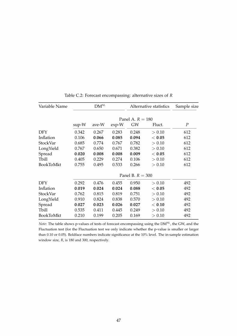
Table C.2: Forecast encompassing: alternative sizes of R

Variable Name DMNL Alternative statistics Sample size

Panel A. R = 180sup-W ave-W exp-W GW Fluct. P

DFY 0.342 0.267 0.283 0.248 > 0.10 612Inflation 0.106 0.066 0.085 0.094 < 0.05 612StockVar 0.685 0.774 0.767 0.782 > 0.10 612LongYield 0.767 0.650 0.671 0.382 > 0.10 612Spread 0.020 0.008 0.008 0.009 < 0.05 612Tbill 0.405 0.229 0.274 0.106 > 0.10 612BookToMkt 0.755 0.495 0.533 0.266 > 0.10 612

Panel B. R = 300

DFY 0.292 0.476 0.455 0.950 > 0.10 492Inflation 0.019 0.024 0.024 0.088 < 0.05 492StockVar 0.762 0.815 0.819 0.751 > 0.10 492LongYield 0.910 0.824 0.838 0.570 > 0.10 492Spread 0.027 0.023 0.026 0.027 < 0.10 492Tbill 0.535 0.411 0.445 0.249 > 0.10 492BookToMkt 0.210 0.199 0.205 0.169 > 0.10 492

Note: The table shows p-values of tests of forecast encompassing using the DMNL, the GW, and theFluctuation test (for the Fluctuation test we only indicate whether the p-value is smaller or largerthan 0.10 or 0.05). Boldface numbers indicate significance at the 10% level. The in-sample estimationwindow size, R, is 180 and 300, respectively.

47

Table C.3: Testing for state dependence: including the indicator as a linear controlvariable

Variable Name DMNL Alternative statistics Sample size

Panel A. Loss differentialsup-W ave-W exp-W GW Fluct. P

DFY 0.565 0.758 0.721 0.523 < 0.10 552Inflation 0.790 0.904 0.904 0.602 > 0.10 552StockVar 0.281 0.194 0.214 0.238 > 0.10 552LongYield 0.846 0.783 0.817 0.700 > 0.10 552Spread 0.144 0.021 0.054 0.570 > 0.10 552Tbill 0.808 0.885 0.891 0.896 > 0.10 552BookToMkt 0.383 0.129 0.204 0.070 < 0.10 552

Panel B. Forecast encompassingsup-W ave-W exp-W GW Fluct. P

DFY 0.324 0.414 0.443 0.416 > 0.10 552Inflation 0.430 0.441 0.466 0.054 < 0.05 552StockVar 0.384 0.342 0.349 0.504 > 0.10 552LongYield 0.709 0.515 0.561 0.260 > 0.10 552Spread 0.011 0.000 0.003 0.002 < 0.05 552Tbill 0.489 0.263 0.343 0.073 > 0.10 552BookToMkt 0.574 0.192 0.287 0.163 > 0.10 552

Note: The table shows p-values of tests of equal predictive ability (Panel A) and forecast encompassing(Panel B) using the DMNL, the GW, and the Fluctuation test (for the Fluctuation test we only indicatewhether the p-value is smaller or larger than 0.10 or 0.05). When using the DMNL test, we additionallyincluded the indicator variable St (monthly real GDP growth), as a linear control. Boldface numbersindicate significance at the 10% level. The in-sample estimation window size, R, is 240.

48

D Additional results: industrial production forecasts

Table D.1: Loss differential: alternative sizes of R

Variable Name DMNL p-values Alternative Statistics Sample Size

Panel A. R = 60

sup-W ave-W exp-W GW Fluct. PHousing Starts 0.079 0.208 0.102 0.731 > 0.10 587VacancyToUr 0.061 0.033 0.037 0.050 > 0.10 587Employment 0.389 0.749 0.643 0.820 > 0.10 587New Orders 0.018 0.043 0.033 0.068 < 0.10 587Consumer Credit 0.187 0.142 0.154 0.054 > 0.10 587One Year Spread 0.871 0.925 0.921 0.951 > 0.10 587Ten Year Spread 0.486 0.390 0.436 0.178 > 0.10 587Credit Spread 0.670 0.591 0.602 0.811 > 0.10 587

Panel B. R = 180

sup-W ave-W exp-W GW Fluct. PHousing Starts 0.049 0.057 0.055 0.538 > 0.10 538VacancyToUr 0.045 0.072 0.056 0.212 < 0.05 538Employment 0.235 0.504 0.454 0.725 > 0.10 538New Orders 0.115 0.182 0.195 0.155 > 0.10 538Consumer Credit 0.001 0.005 0.003 0.040 > 0.10 538One Year Spread 0.417 0.584 0.585 0.441 > 0.10 538Ten Year Spread 0.551 0.736 0.737 0.529 > 0.10 538Credit Spread 0.327 0.267 0.281 0.188 > 0.10 538

Note: The table shows p-values of tests of equal predictive ability using the DMNL, the GW, and theFluctuation test (for the Fluctuation test we only indicate whether the p-value is smaller or larger than0.10 or 0.05). Boldface numbers indicate significance at the 10% level. The in-sample estimation windowsize, R, is 60 and 180, respectively.

49

Table D.2: Testing for state dependence: including the indicator as a linear controlvariable

Variable Name DMNL p-values Alternative statistics Sample Size

sup-W ave-W exp-W GW Fluct. PHousing Starts 0.335 0.262 0.270 0.641 > 0.10 587VacancyToUr 0.163 0.043 0.096 0.045 > 0.10 587Employment 0.386 0.395 0.444 0.362 > 0.10 587New Orders 0.136 0.053 0.102 0.039 > 0.10 587Consumer Credit 0.098 0.046 0.057 0.020 > 0.10 587One Year Spread 0.329 0.703 0.644 0.430 > 0.10 587Ten Year Spread 0.374 0.473 0.462 0.422 > 0.10 587Credit Spread 0.663 0.809 0.804 0.740 > 0.10 587

Note: The table shows p-values of tests of equal predictive ability using the DMNL, the GW, and theFluctuation test (for the Fluctuation test we indicate whether the p-value is smaller or larger than 0.10 or0.05). When using the DMNL test, we additionally included the indicator variable St (ANFCI), as a linearcontrol. Boldface numbers indicate significance at the 10% level. The in-sample estimation window size,R, is 120.

50