evaluating interest rate covariance models within a value ...€¦ · evaluating interest rate...
TRANSCRIPT
Evaluating Interest Rate Covariance Models within a
Value-at-Risk Framework∗
Miguel A. Ferreira†
ISCTE School of Business
Jose A. Lopez‡
Federal Reserve Bank of San Francisco
This Version: March 2004
First Version: May 2003
∗ Please note that the views expressed here are those of the authors and not necessarily those of theFederal Reserve Bank of San Francisco or of the Federal Reserve System.
†Address: ISCTE Business School - Lisbon, Complexo INDEG/ISCTE, Av. Prof. Anibal Bettencourt,1600-189 Lisboa, Portugal. Phone: 351 21 7958607. Fax: 351 21 7958605. E-mail: [email protected].
‡Address: Economic Research Department Group Risk Management, Federal Reserve Bank of San Fran-cisco, 101 Market Street, San Francisco, CA 94705. Phone: (415) 977-3894. Fax: (415) 974-2168. E-mail:[email protected].

Abstract
We find that covariance matrix forecasts for an international interest rate portfolio generated by a
model that incorporates interest-rate level volatility effects perform best with respect to statistical
loss functions. However, within a value-at-risk (VaR) framework, the relative performance of the
covariance matrix forecasts depends greatly on the VaR distributional assumption. Simple forecasts
based just on weighted averages of past observations perform best using a VaR framework. In fact,
we find that portfolio variance forecasts that ignore the individual assets in the portfolio generate
the lowest regulatory capital charge, a key economic decision variable for commercial banks. Our
results provide empirical support for the commonly-used VaR models based on simple covariance
matrix forecasts and distributional assumptions.
JEL classification: C52; C53; G12; E43
Keywords: Interest rates; Covariance models; GARCH; Forecasting; Risk Management, Value-at-
Risk

1 Introduction
The short-term interest rate is one of the most important and fundamental variables in financial
markets. In particular, interest rate volatility and its forecasts are important to a wide variety
of economic agents. For example, portfolio managers require such volatility forecasts for asset
allocation decisions; option traders require them to price and hedge interest rate derivatives; and
risk managers use them to compute measures of portfolio market risk, such as value-at-risk (VaR).
In fact, since the late 1990s, financial regulators have been using VaR methods and their underlying
volatility forecasts to supervise and monitor the trading portfolios and interest rate exposures of
financial institutions.
Forecasts of interest rate volatility are available from two general sources. The market-based
approach uses option market data to infer implied volatility, which is interpreted to be the market’s
best estimate of future volatility conditional on an option pricing model. Since these forecasts
incorporate the expectations of market participants, they are said to be forward-looking measures.
The model-based approach forecasts volatility from time series data, generating what are usually
called historical forecasts. The empirical evidence in Day and Lewis (1992), Amin and Ng (1997),
and others suggests that implied volatility can forecast future volatility. However, there is also
some consensus that implied volatility is an upward biased forecast of future volatility and that
historical volatility forecasts contain additional information. Moreover, the scope of implied second
moments is limited due to options contracts availability, especially with respect to covariances.1
Most of the work on the model-based approach to forecasting second moments has focused on
univariate time-varying variance models. For examples, see Glosten, Jagannathan, and Runkle
(1993) and Engle and Ng (1993). Most studies evaluate the performance of such volatility models
in-sample analysis, although some have examined their out-of-sample performance using statistical
loss functions; see for example, Pagan and Schwert (1990), West and Cho (1995), and Figlewski
(1997).
Out-of-sample evaluation of forecasts provides an alternative and potentially more useful com-1Campa and Chang (1998) and Walter and Lopez (2000) find that implied correlations from foreign exchange
options tend to be more accurate forecasts of realized correlation than the ones based on historical prices. However,implied correlations do not fully incorporate the information in historical data because bivariate GARCH models ofcorrelation are able to improve forecast accuracy.
1

parison of the alternative models, due to the possibility of overfitting.2 Moreover, the ability to
produce useful out-of-sample forecasts is the clear test of model performance because it only uses
the same information set available to agents at each point in time. Previous studies across a wide
variety of markets have compared the out-of-sample forecasting ability of several GARCH type
models with that of simple variance measures and found that there is no clear winner using sta-
tistical loss functions.3 Results in Figlewski (1997) show that GARCH models fitted to daily data
may be quite useful in forecasting the volatility in stock markets both for short and long horizons,
but they are much less useful in making out-of-sample forecasts in other markets beyond short
horizons4. In particular, using 3-month US Treasury bill yields, sample variances generate more ac-
curate forecasts than GARCH model. Ederington and Guan (1999) also find that sample variances
dominate GARCH models in the 3-month Eurodollar market.
In contrast, relatively little work has been done on modeling and forecasting second moments
using multivariate time-varying covariance models. Kroner and Ng (1998) propose a general family
of multivariate GARCH models, called General Dynamic Covariance (GDC) model, to estimate the
variance-covariance matrix of a portfolio of large and small US stocks. Ferreira (2001) presents a new
multivariate model for interest rates, called the mixed GDC and levels (GDC-Levels) model, which
includes both level effects and conditional heteroskedasticity effects in the volatility dynamics.5
He finds that the interest rate variance-covariance matrix is best forecasted out-of-sample using a
VECH model with a level effect. In addition, simple models using either equally or exponentially-
weighted moving averages of past observations perform as well under statistical loss functions as
the best multivariate model in terms of both variance and covariance. Overall, his out-of-sample
results present evidence that model features often required to obtain a good in-sample fit do not
contribute to out-of-sample forecasting power.
Given the wide variety of volatility models available and their mixed out-of-sample performance2Lopez (2001) finds in the foreign exchange markets that out-of-sample analysis of volatility forecasts is useful
because the best set of forecasts varies not only among foreign exchange rates but also from in-sample to out-of-sampleevaluation. Ederington and Guan (1999) also find evidence supporting that in-sample results may not be confirmedout-of-sample.
3See Andersen and Bollerslev (1998) for further discussion of this point.4This sensitivity of results to the forecast horizon can also be found in West and Cho (1995) with the GARCH model
having a slight advantage for short forecast horizons in foreign exchange markets, but this advantage disappearingfor longer horizons.
5The sensitivity of interest rate volatility to the interest rate level was first documented by Chan, Karolyi, Longstaff,and Sanders (1992).
2
with respect to statistical loss functions, a key question is how to choose among them. A relatively
informative method of model selection is to compare their out-of-sample performance in terms
of a particular economic application and results may vary according to the selected economic loss
function; see for example Lopez (2001). However, there has been relatively little work on comparing
the out-of-sample performance of alternative models in terms of economic loss functions, especially
in a multivariate framework.
To date, such economic evaluations of out-of-sample volatility forecasts has been in the areas of
hedging performance, asset allocation decisions and options pricing. Regarding hedging strategies,
Cecchetti, Cumby, and Figlewski (1988) find that a time-varying covariance matrix is necessary to
construct an optimal hedge ratio between Treasury bonds and bond futures, while Kroner and Ng
(1998) find that the choice of the multivariate specification can result in very different estimates
of the optimal hedge ratio for stock portfolios. With respect to asset allocation, volatility model
selection is also important as shown by Kroner and Ng (1998) in the context of a portfolio of
small and large stocks. Poomimars, Cadle, and Theobald (2001) also find that for the purposes of
allocating assets across national stock markets, simpler models of the covariance matrix are more
appropriate when optimizing across asset universes that include less stable national markets and
environments. For options pricing, Engle, Kane, and Noh (1997) and Gibson and Boyer (1998) find
that standard time-series models produce better correlation forecasts than simple moving average
models for the purpose of stock-index option pricing and trading. Christoffersen and Jacobs (2002)
also evaluate alternative GARCH covariance forecasts in terms of option pricing and finds out-of-
sample evidence in favor of a relatively parsimonious model.
In this paper, we consider economic loss functions related to financial risk management, which
places emphasis on value-at-risk (VaR) measures that generally indicate the amount of portfolio
value that could be lost over a given time horizon with a specified probability. Hendricks (1996)
provides the most extensive evaluation of alternative VaR models using a portfolio of foreign ex-
change rates, although he does not examine covariance matrix forecasts. Other papers — Dave and
Stahl (1996), Alexander and Leigh (1997), and Jackson, Maude, and Perraudin (1997) — examine
VaR measures for different asset portfolios using multivariate models. We extend this literature by
evaluating the forecast performance of multivariate volatility models within a VaR framework and
using interest rate data, as per Lopez and Walter (2001) and Vlaar (2000), respectively.
3

The performance of VaR for interest rate portfolios, one of the most important financial prices
and of particular relevance in banks’ trading portfolios6, has only been studied using univariate
models. Vlaar (2000) examines the out-of-sample forecast accuracy of several univariate volatility
models (equally and exponentially sample averages as well as GARCH models) for portfolios of
Dutch bonds with different maturities. In addition, he examines the impact of alternative VaR
distributional assumptions. The analysis shows that the percentage of exceedances for the sim-
ple models is basically equal to that for the GARCH models. The distributional assumption is
important with the normal performing much better than the t-distribution.
In this paper, we analyze an equally-weighted portfolio of short-term fixed income positions in
the US dollar, German deutschemark and Japanese yen. The portfolio returns are calculated from
the perspective of a US-based investor using daily interest rate and foreign exchange data from
1979 to 2000. We examine VaR estimates for this portfolio from a wider variety of multivariate
volatility models, ranging from simple sample averages to standard time-series models. We compare
the out-of-sample forecasting performance of these alternative variance-covariance structures and
their economic implications within the VaR framework used by Lopez and Walter (2001). The
question of interest is whether more complex covariance models provide improved out-of-sample
VaR forecasts.
The VaR framework we use consists of three sets of evaluation techniques. The first set focuses
on the statistical properties of VaR estimates derived from alternative covariance matrix forecasts
and VaR distributional assumptions. Specifically, the binomial test of correct unconditional and
conditional coverage, which is implicitly incorporated into the aforementioned bank capital require-
ments, is used to examine 1%, 5%, 10% and 25% VaR estimates.
The second set of techniques focus on the magnitude of the losses experienced when VaR
estimates are exceeded, clearly an issue of interest to financial institutions and their regulators. To
determine whether the magnitudes of observed exceptions are in keeping with the model generating
the VaR estimates, we use the hypothesis test based on the truncated normal distribution proposed
by Berkowitz (2001).
Finally, to examine the performance of the competing covariance matrix forecasts with respect6Berkowitz and O’Brien (2002) report that the poor performance of banks trading portfolios during the 1998-2000
period is mainly due to interest rate positions.
4

to regulatory capital requirements, we use the regulatory loss function implied by the U.S. imple-
mentation of the market risk amendment to the Basel Capital Accord. This loss function penalizes
a VaR model for poor performance by using a capital charge multiplier based on the number of
VaR exceptions; see Lopez (1999b) for further discussion.
Our findings are roughly in line with those of Lopez and Walter (2001), which were based on a
simple portfolio of foreign exchange positions. As per Ferreira (2001), we confirm that covariance
matrix forecasts generated from models that incorporate interest-rate level effect perform best under
statistical loss functions. However, within a VaR framework, we find that the relative performance
of covariance matrix forecasts depends greatly on the VaR models’ distributional assumptions. Of
the VaR forecasts examined, simple specifications, such as exponentially-weighted moving averages
of past observations, perform best with regard to the magnitude of VaR exceptions and regula-
tory capital requirements. Our results provide further empirical support for the commonly-used
VaR models based on simple covariance matrix forecasts and distributional assumptions, such as
the normal and the nonparametric distributions. Moreover, simple variance forecasts based only
on the portfolio returns (i.e., ignoring the portfolio’s component assets) perform as well as the
best covariance forecasts of individual portfolio assets’ and, in fact, generate the minimum capital
requirements in our exercise.
These findings are also mainly consistent with the evidence in Berkowitz and O’Brien (2002),
who analyzed the daily trading revenues and VaR estimates of six US commercial banks. They
conclude that these VaR estimates are too high, but that losses do significantly exceed the VaR
estimates at times within their sample period. They also find that a GARCH model of portfolio
returns that ignores the component assets, when combined with a normal distributional assumption,
provides VaR estimates and regulatory capital requirements that are comparable to other models
and does not produce such large VaR exceptions. Our results based on fixed portfolio weights
provide evidence that the Berkowitz and O’Brien (2002) finding is not explained by an offset
between the static portfolio weights (i.e., current portfolio weights overestimate future portfolio
weights if traders react to changes in volatility by adjusting their portfolio holdings in order to
minimize risk) and the neglected leptokurtosis of the portfolio return distribution.
The paper is structured as follows. Section 2 describes the issue of forecasting variances and
covariances and presents the alternative time-varying covariance specifications. We also compare
5

the models in terms of out-of-sample forecasting power for variances and covariances. Section 3
describes the VaR models analyzed. Section 4 presents the results for the hypothesis tests that
make up the VaR evaluation framework. Section 5 concludes.
2 Time-Varying Covariance Models
In this paper, we study an equally-weighted US dollar-denominated portfolio of three month US
dollar (US$), Deutschemark (DM) and Japanese yen (JY) interest rates. We take the view of a US-
based investor, who is unhedged with respect to exchange rate risk. Thus, we need to estimate the
(5x5) variance-covariance matrix between the three interest rates as well as DM/US$ and JY/US$
exchange rates.
2.1 Forecasting Variances and Covariances
The empirical model for the short-term interest rates rit is given by, for i =US$,DM,JP,
rit − rit−1 = µi + κirit−1 + εit, (1)
and for the foreign exchange rate sit, for i =DM/US$,JY/US$,
ln
µsitsit−1
¶= εit, (2)
with E [εit|Ft−1] = 0 and where Ft−1 is the information set up to time t− 1. The conditional meanfunction for the interest rate in (1) is given by a first order autoregressive process and we assume
a zero conditional mean for the continuously compounded foreign exchange rate of return in (2).
The conditional variance-covariance matrix Ht is (5× 5) with elements [hijt] . The conditionalcovariance can be expressed as
hijt = E [εitεjt|Ft−1] , (3)
and the conditional correlation is given by
6
ρijt =E [εitεjt|Ft−1]p
E [εit|Ft−1]E [εjt|Ft−1]=
hijtphiithjjt
. (4)
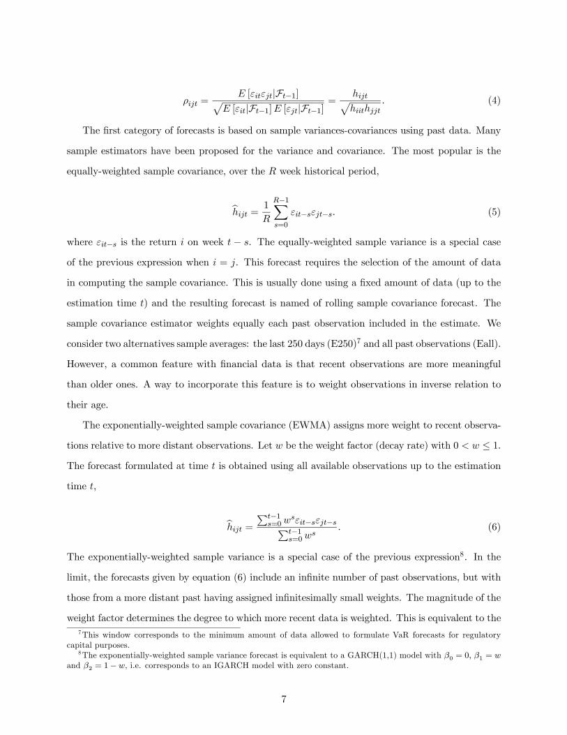
The first category of forecasts is based on sample variances-covariances using past data. Many
sample estimators have been proposed for the variance and covariance. The most popular is the
equally-weighted sample covariance, over the R week historical period,
bhijt = 1
R
R−1Xs=0
εit−sεjt−s. (5)
where εit−s is the return i on week t − s. The equally-weighted sample variance is a special caseof the previous expression when i = j. This forecast requires the selection of the amount of data
in computing the sample covariance. This is usually done using a fixed amount of data (up to the
estimation time t) and the resulting forecast is named of rolling sample covariance forecast. The
sample covariance estimator weights equally each past observation included in the estimate. We
consider two alternatives sample averages: the last 250 days (E250)7 and all past observations (Eall).
However, a common feature with financial data is that recent observations are more meaningful
than older ones. A way to incorporate this feature is to weight observations in inverse relation to
their age.
The exponentially-weighted sample covariance (EWMA) assigns more weight to recent observa-
tions relative to more distant observations. Let w be the weight factor (decay rate) with 0 < w ≤ 1.The forecast formulated at time t is obtained using all available observations up to the estimation
time t,
bhijt = Pt−1s=0w
sεit−sεjt−sPt−1s=0w
s. (6)
The exponentially-weighted sample variance is a special case of the previous expression8. In the
limit, the forecasts given by equation (6) include an infinite number of past observations, but with
those from a more distant past having assigned infinitesimally small weights. The magnitude of the
weight factor determines the degree to which more recent data is weighted. This is equivalent to the7This window corresponds to the minimum amount of data allowed to formulate VaR forecasts for regulatory
capital purposes.8The exponentially-weighted sample variance forecast is equivalent to a GARCH(1,1) model with β0 = 0, β1 = w
and β2 = 1−w, i.e. corresponds to an IGARCH model with zero constant.
7

exponential smoother proposed in the Riskmetrics. The exponentially-weighted forecast requires
the estimation of the weight factor w. We assume a weight factor w = 0.94, which it is identical to
the one commonly used in practice (e.g. Riskmetrics).
We also consider forecasts based directly on the portfolio returns, which ignore the covariance
matrix specification completely. This approach significantly reduces the computational time (and
estimation errors) and presents comparable performance in terms of VaR as reported in Lopez
and Walter (2001) and Berkowitz and O’Brien (2002). In particular, we examine the equally-
weighted (with 250 and all past observations) and exponentially-weighted (with a decay factor of
0.94) sample variance of portfolio returns and denote them of E250 Portfolio, Eall Portfolio, and
EWMA Portfolio, respectively. We also consider a GARCH(1,1) variance model of portfolio return,
denoted GARCH Portfolio.
Multivariate GARCH models are a natural extension of the previous methods and are among
the most widely used time-varying covariance models. In the basic multivariate GARCH model, the
components of the conditional variance-covariance matrix Ht vary through time as functions of the
lagged values of Ht and of the squared innovations, εt is (5×1) vector of innovations. We model theUS$, DM and JP short-term interest rates as well as DM/US$ and JY/US$ foreign exchange rates
using a multivariate GARCH(1,1) structure because this process is able to successfully represent
most financial time series. We implement several (but not all) multivariate GARCH specifications
that have been suggested in the literature as we will discuss below.9
2.1.1 VECH Model
The VECH model of Bollerslev, Engle, and Wooldridge (1988) is a parsimonious version of the
most general multivariate GARCH model, and is given by, for i, j = 1, 2, ..., 5,
hijt = ωij + βijhijt−1 + αijεit−1εjt−1, (7)
where ωij , βij and αij are parameters. The VECH model is simply an ARMA process for εitεjt.
The covariance is estimated using geometrically declining weighted averages of past cross products
of innovations to the interest rate process. An implementation problem is that the model may not9A notable exception is the recently proposed DCC model by Engle (2002).
8

yield a positive definite covariance matrix. The VECH model does not allow for volatility spillover
effects, i.e. the conditional variance of a given variable is not a function of other variable shocks
and past variance.
2.1.2 Constant Correlation (CCORR) Model
In the CCORR model of Bollerslev (1990), the conditional covariance is proportional to the product
of the conditional standard deviations. Consequently, the conditional correlation is constant across
time. The model is described by the following equations, for i, j = 1, 2, ..., 5,
hiit = ωii + βiihiit−1 + αiiε2it−1, hijt = ρij
phiit−1
phjjt−1, for all i 6= j. (8)
The conditional covariance matrix of the CCORR model is positive definite if and only if the
correlation matrix is positive definite. Like in the VECH model there is no volatility spillover
effects across series.
2.1.3 BEKK Model
The BEKK model of Engle and Kroner (1995) addresses the problem of the estimated conditional
covariance matrix being positive definite. The model is given by:
Ht = Ω+B0Ht−1B +A0εt−1ε0t−1A, (9)
where Ω, A, and B are (5× 5) matrices, with Ω symmetric. In the BEKK model, the conditionalcovariance matrix is determined by the outer product matrices of the vector of past innovations.
As long as Ω is positive definite, the conditional covariance matrix is also positive definite because
the other terms in (9) are expressed in quadratic form.
2.1.4 General Dynamic Covariance (GDC) Model
The GDCmodel proposed by Kroner and Ng (1998) nests many of the existing multivariate GARCH
models. The conditional covariance specification is given by:
Ht = DtRDt +Φ Θt, (10)
9
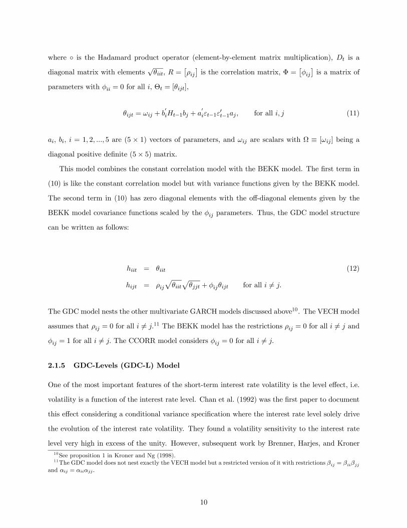
where is the Hadamard product operator (element-by-element matrix multiplication), Dt is adiagonal matrix with elements
√θiit, R =
£ρij¤is the correlation matrix, Φ =
£φij¤is a matrix of
parameters with φii = 0 for all i, Θt = [θijt],
θijt = ωij + b0iHt−1bj + a
0iεt−1ε
0t−1aj , for all i, j (11)
ai, bi, i = 1, 2, ..., 5 are (5 × 1) vectors of parameters, and ωij are scalars with Ω ≡ [ωij ] being adiagonal positive definite (5× 5) matrix.
This model combines the constant correlation model with the BEKK model. The first term in
(10) is like the constant correlation model but with variance functions given by the BEKK model.
The second term in (10) has zero diagonal elements with the off-diagonal elements given by the
BEKK model covariance functions scaled by the φij parameters. Thus, the GDC model structure
can be written as follows:
hiit = θiit (12)
hijt = ρijpθiitpθjjt + φijθijt for all i 6= j.
The GDC model nests the other multivariate GARCH models discussed above10. The VECH model
assumes that ρij = 0 for all i 6= j.11 The BEKK model has the restrictions ρij = 0 for all i 6= j andφij = 1 for all i 6= j. The CCORR model considers φij = 0 for all i 6= j.
2.1.5 GDC-Levels (GDC-L) Model
One of the most important features of the short-term interest rate volatility is the level effect, i.e.
volatility is a function of the interest rate level. Chan et al. (1992) was the first paper to document
this effect considering a conditional variance specification where the interest rate level solely drive
the evolution of the interest rate volatility. They found a volatility sensitivity to the interest rate
level very high in excess of the unity. However, subsequent work by Brenner, Harjes, and Kroner10See proposition 1 in Kroner and Ng (1998).11The GDC model does not nest exactly the VECH model but a restricted version of it with restrictions βij = βiiβjj
and αij = αiiαjj .
10

(1996) show that the level effect exists but it is considerably smaller (consistent with a square root
process) by incorporating in the variance function both level and conditionally heteroskedasticity
effect (news effect) in a GARCH framework. Bali (2003) also finds that incorporating both GARCH
and level effects in the interest rate volatility specifications improves the pricing performance of
the models. Here, we consider a multivariate version of the Brenner et al. (1996) model combining
a multivariate GARCH model with the level effec.
The GDC model of Kroner and Ng (1998) can be extended to incorporate level effect in the
variance-covariance function for the interest rates (not for the exchange rates),
θijt = ω∗ij + b0iH
∗t−1bj + a
0iε∗t−1ε
∗0t−1aj , for i, j = 1, 2, 3 (13)
where ω∗ii = ωii/r2γiit−1, the diagonal elements of the matrix H
∗t−1 are multiplied by the factor
(rit−1/rit−2)2γi for all i, and the elements of the vector ε∗t−1 are divided by rγiit−1 for all i. The GDC-
Levels model nests the other multivariate GARCH models combined with level effect. The exact
form of conditional variance in the VECH model with level effect (VECH-Levels model, VECH-L)
for the interest rates is given by:
hiit =³ωii + βiihiit−1r
−2γiit−2 + αiiε
2it−1
´r2γiit−1. (14)
The CCORR model with level effect (CCORR-Levels, CCORR-L) will also have a variance function
given by the equation (14) and the covariance function is defined as before. Similarly, we also
incorporate level effect within the BEKK specification (BEKK-Levels model, BEKK-L).
2.2 Models Estimation
2.2.1 Data Description
The interest rate data consists of US dollar (US$), Deutschemark (DM) and Japanese yen (JY) Lon-
don interbank money market three-month interest rates (middle rate) obtained from Datastream
(codes ECUSD3M, ECWGM3M and ECJAP3M, respectively).12 The interest rates are given in
percentage and in annualized form. These interest rates are taken as proxies for the instantaneous12The only exception is the JY interest rate in the period from January 1995 to December 2000 in which we use
the three-month offered rate (code JPIBK3M).
11

riskless interest rate (i.e., the short rate). We also require foreign exchange rates to compute U.S.
dollar investor rates of return. The exchange rate market data includes JY per US$ (denoted
JY/US$) and DM per US$ (denoted DM/US$) spot exchange rates in the London market also
from Datastream.13
The frequency is daily and covers the period from January 12, 1979 to December 29, 2000,
providing 5731 observations in total. Table 1 presents summary statistics for the interest and
exchange rates. The daily mean interest rate changes are close to zero. The daily interest rate
changes standard deviation differ considerably across countries with the US dollar interest rate
having an annualized standard deviation of 2.8% compared with 1.8% and 1.4% for the Japanese
and German interest rates, respectively. Foreign exchange rates present a much higher degree of
variation with an annualized standard deviation of about 11% for both series. Table 1 also presents
summary statistics for an equally-weighted portfolio of the US$, DM and JY interest rates with
returns calculated in US$ (see section 3 for a detailed portfolio definition). The mean portfolio
return is close to zero with an annualized standard deviation of 19.6%. The portfolio return
presents leptokurtosis, though less severe that most individual components series, with exception
of the DM/US$ exchange rate return.
As in most of the literature, we focus on nominal interest rates because defining real interest
rates, especially at high frequencies, is subject to serious measurement errors. The use of daily
frequency minimizes the discretization bias resulting from estimating a continuous-time process
using discrete periods between observations. On the other hand, the use of a three-month rate
maturity proxy for the instantaneous interest rate is unlikely to create a significant proxy bias as
shown in Chapman, Long, and Pearson (1999). Finally, we use interbank interest rates instead
of Treasury bill yields because of the low liquidity of the Treasury bill secondary market in both
Germany and Japan, in sharp contrast with the high liquidity of the interbank money market. The
concern regarding the existence of a default premium in the interbank money market should not
be severe since these interest rates result from trades among high-grade banks that are considered
almost default-free.13For earlier years of the sample, the direct per US$ quotes are not available, but we construct the series from
British pound (BP) exchange rates quoted by WM/Reuters (US$ per BP, DM per BP and JY per BP rates).
12
2.2.2 Forecasting Performance
We estimate the multivariate models parameters using the period from January 12, 1977 to Decem-
ber 29, 1989 (2861 daily observations) to calculate the models’ one-step-ahead variance-covariance
forecasts over the out-of-sample period from January 1, 1990 and December 29, 2000 (2870 obser-
vations). We use a fixed scheme to estimate the multivariate models’ parameters, i.e. we do not
reestimate the parameters as we move forward in the out-of-sample period.
Following standard practices, we estimate the models by maximizing the likelihood function
under the assumption of independent and identically distributed (i.i.d.) innovations. In addition, we
assume that the conditional density function of the innovations is given by the normal distribution.
Conditional normality of the innovations is often difficult to justify in many empirical applications
that use leptokurtic financial data. However, the maximum likelihood estimator based on the
normal density has a valid quasi-maximum likelihood (QML) interpretation as shown by Bollerslev
and Wooldridge (1992).14
Tables 2 and 3 presents models’ out-of-sample forecasting performance in terms of root mean
squared prediction error (RMPSE). Table 2 reports RMSPE for the variances of the five component
assets and the overall portfolio, and Table 3 reports RMSPE for ten relevant covariances. We also
report the Diebold and Mariano (1995) test statistic comparing the models’ forecasting accuracy
relative to the one with the minimum RMSPE.
Overall, the best performing interest rate volatility models are the VECH and CCORR models
with a level effect; note that including volatility spillover effects is not important. The null hypoth-
esis that the VECH-Levels and CCORR-Levels models perform similarly to the best forecast is only
rejected at the 5% level in 3 and 2 cases out of 15 cases (i.e., five variances and ten covariances),
respectively. The VECH-Levels and CCORR-Levels model are among the two best performing
models in 6 and 4 cases, respectively.
A simple model using equally-weighted moving averages of past 250 observations (E250) per-
forms similarly to the best multivariate models, especially in terms of covariance. Also, the
exponentially-weighted moving average (EWMA) forecast also performs quite well for variances,
though for covariances presents low accuracy in some cases. The null hypothesis of equality between14Model parameters are not presented here in order to conserve space, but they are available from the authors
upon request.
13

this forecast and the minimizing forecast is only rejected at the 5% level in 3 cases and it is one of
the two RMSPE minimizing forecasts in 8 cases out of 15 cases.
The worst performing models are the GDC and GDC-Levels models, which are the most general
specifications and indicate that they tend to overfit the data in-sample. The GDC-Levels model
is rejected in 9 cases at the 5% level and in 3 cases (out of 15) at the 10% level in terms of
generating forecasts with similar performance to the best model. Among the simple models, the
equally-weighted moving average of all past observations (Eall) presents the worst performance
being rejected at the 5% level in 13 cases out of 15 cases.
The model selection is more important for forecasting interest rates variance, especially for the
US, than for forecasting exchange rates volatility. Also, the performance of covariance forecasts are
more sensitive to model selection than the performance of variance forecasts.
With respect to the portfolio variance, it is best forecast by the VECH-Levels model confirming
the models forecasting performance in terms of individual variances and covariances. The null
hypothesis of equal forecasting power relative to the best model is not rejected for the portfolio
variance forecasts that are based directly on the portfolio returns (GARCH Portfolio and EWMA
Portfolio). This result indicates that simple portfolio variance forecasts are useful, but that forecasts
based on covariance matrix specifications generally perform as well or better. Surprisingly, the
equally-weighted moving averages of past 250 observations forecast (E250) is rejected in terms of
forecasting portfolio variance, in contrast with its good performance for individual variances and
covariances.
In summary, statistical loss functions provide a useful, although incomplete, analysis of indi-
vidual assets’ variance and covariance as well as portfolio variance forecasts. Our results indicate
that the second moment forecasts from simple models and time-varying covariance models present
similar out-of-sample forecasting performance. In addition, the most complex time-varying covari-
ance models tend to overfit the data. Our findings are generally consistent with those of Ferreira
(2001) for interest rates, and West and Cho (1995) and Lopez (2001) for exchange rates. However,
economic loss functions that explicitly incorporate the costs faced by volatility forecast users pro-
vide the most meaningful forecast evaluations. In the next section, we examine the performance of
the covariance matrix forecasts within a value-at-risk framework.
14

3 Value-at-Risk Framework
3.1 Portfolio Definition
Assume that we have a US fixed-income investor managing positions in US$, DM, and JY zero-
coupon bonds15 in terms of dollar-denominated returns16. The value of a zero-coupon bond with
unit face value and a three-month maturity at time t+ 1 is given by
PUS$t+1 = e− 14rUS$t+1 , (15)
where rUS$t+1 is the continuously compounded three-month interest rate (annualized). Define the
value of a US$ investment tomorrow to be
YUS$t+1 = YUS$teRUS$t+1 , (16)
where RUS$t+1 denotes the day t+1 geometric rate of return on the three-month zero-coupon bond
investment. In the US case, YUS$t+1 = PUS$t+1, hence
RUS$t+1 = −1
4(rUS$t+1 − rUS$t) . (17)
The value of the DM zero-coupon bond in US$ tomorrow is given by:
YDMt+1 =¡YDMtsDM/US$t
¢eRDM it+1sUS$/DMt+1, (18)
where sUS$/DMt is the exchange rate between US$ and DM. Thus, the day t+ 1 geometric rate of
return on the DM three-month zero-coupon bond investment given by:
ln (YDMt+1)− ln (YDMt) = RDMt+1 −∆ ln¡sDM/US$t+1
¢, (19)
15We use bond returns implied by interbank money market rates (LIBOR) instead of bond returns. This is commonto other studies such as Duffie and Singleton (1997) and presents several advantages. First, the interbank moneymarket is more liquid than the Treasury bill market in most countries. Second, most interest rate derivatives arepriced using interbank interest rates. Third, credit risk minimally affects these rates as they are subject to specialcontractual netting features and correspond to trades among high-grade banks.16We take the perspective of a US-based investor, who is unhedged with respect to exchange rate risk.
15
where RDMt+1 = −14 (rDMt+1 − rDMt) is the local-currency rate of return on the fixed incomeinvestment and ∆ ln
¡sDM/US$t+1
¢=£ln¡sDM/US$t+1
¢− ln ¡sDM/US$t¢¤ is the foreign exchange rateof return. The analysis for the JY fixed income position is the same as for the DM fixed income,
with the geometric rate of return on the JY three-month zero-coupon bond investment given by
ln (YJYt+1)− ln (YJYt) = RJYt+1 −∆ ln¡sJY/US$t+1
¢, (20)
where RJYt+1 = −14 (rJYt+1 − rJYt) and ∆ ln¡sJY/US$t+1
¢=£ln¡sJY/US$t+1
¢− ln ¡sJY/US$t¢¤ .For simplicity, we will assume that the portfolio at time t is evenly divided between the three
fixed-income positions (equally-weighted portfolio). Thus, the investor’s market risk exposure is to
the sum of the three investment returns. That is,
Rpt+1 =
·RUS$t+1 RDMt+1 ∆ ln
¡sDM/US$t+1
¢RJYt+1 ∆ ln
¡sJY/US$t+1
¢ ¸w0, (21)
where w =·1 1 −1 1 −1
¸is the portfolio weight vector.
3.2 VaR Models and Exceptions
We examine the accuracy of several VaR models based on different covariance matrix specifications
and conditional densities. A VaR estimate on day t is a specified quantile of the forecasted return
distribution ft+k over a given holding period k. The VaR estimate at time t derived from model
m for a k-period-ahead return, denoted VaRmt(k,α), is the critical value that corresponds to the
lower α percent tail of the distribution,
VaRmt(k,α) = F−1mt+k(α) (22)
where F−1mt+k is the inverse of the cumulative distribution function to fmt+k. A VaRmodelm consists
of two items: a covariance matrix model and a univariate distributional assumption. Following
Lopez and Walter (2001), we separately specify the portfolio variance dynamics
hmpt+1 = w0Hmt+1w, (23)
16

and the distribution form of fmt+k.17 In terms of portfolio variance dynamics we consider eight
multivariate covariance model forecasts, three sample variance forecast and four portfolio variance
forecasts, in a total of 15. In terms of distributions we consider four alternative assumptions:
normal, t-student, generalized t-student, and nonparametric distribution. This gives a total of
60 VaR models. The last distributional form is the unsmoothed distribution of the standardized
portfolio returns residuals, which is the distribution used in the so-called “historical simulation”
approach for generating VaR estimates.
The t-distribution assumption requires an estimate of the number of degrees of freedom, which
affects the tail thickness of the distribution. This parameter is estimated using the in-sample stan-
dardized residuals generated by the 15 model specifications. The estimated number of degrees
of freedom ranges from 8 and 11, which correspond to some fat taildness, and the implied 1%
quantiles range from -2.9 to -2.7 compared with -2.33 for the normal distribution. The generalized
t-distribution assumption requires estimates of two parameters that control the tail thickness and
width of the center of the distribution, named n and q. The parameters n and q are also estimated
using the in-sample standardized residuals and are found to be approximately to 2.5 and 1, respec-
tively. These estimates imply considerable more fat taildness than the normal distribution at the
1% quantile (-3.27), but the reverse is true at the higher quantiles.
The nonparametric distribution quantiles are estimated using the unsmoothed distribution of
the standardized portfolio return residuals arising from each of the 15 models. The estimated
nonparametric critical values generally present more fat-taildness at the 1% and 5% quantiles than
the normal distribution, but the opposite is true at the higher quantiles.
The one-day-ahead VaR estimates from model m for the portfolio at the α quantile on day t is
VaRmt (α) =phmpt+1F
−1m (α) , (24)
where we drop the subscript t from the portfolio distribution because we assume that it is constant
across time. We then compare VaRmt (α) to the actual portfolio return on day t + 1, denoted17The intuition for specifying a VaR model as a separate portfolio variance (whether based on a modeled covariance
matrix or portfolio variance) and a distributional assumption arises from the two-step procedure proposed by Engleand Gonzalez-Rivera (1991). Note that an alternative approach is to estimate the parameters of a multivariatevolatility model using a distributional form other than the multivariate normal. However, such distributional formsare difficult to specify and use in estimation.
17

as Rpt+1. If Rpt+1 <VaRmt (α), then we have an exception. For testing purposes, we define the
exception indicator variable as
Imt+1 =
1 if Rpt+1 < VaRmt (α)
0 if Rpt+1 ≥ VaRmt (α). (25)
3.3 VaR Evaluation Tests
3.3.1 Unconditional and Conditional Coverage Tests
Assuming that a set of VaR estimates and their underlying model are accurate, exceptions occur
when Rpt+1 <VaRmt (α) , and they can be modeled as independent draws from a binomial distrib-
ution with a probability of occurrence equal to α percent. Accurate VaR estimates should exhibit
the property that their unconditional coverage bα = x/T equals α percent, where x is the numberof exceptions and T the number of observations. The likelihood ratio statistic for testing whether
bα = α is
LRuc = 2hlog³bαx (1− bα)T−x´− log³αx (1− α)T−x
´i, (26)
which has an asymptotic χ2 (1) distribution.18
The LRuc test is an unconditional test of the coverage of VaR estimates since it simply counts
exceptions over the entire period without reference to the information available at each point in
time. However, if the underlying portfolio returns exhibit time-dependent heteroskedasticity, the
conditional accuracy of VaR estimates is probably a more important issue. In such cases, VaR
models that ignore such variance dynamics will generate VaR estimates that may have correct
unconditional coverage, but at any given time, will have incorrect conditional coverage.
To address this issue, Christoffersen (1998) proposed conditional tests of VaR estimates based
on interval forecasts. VaR estimates are essentially interval forecasts of the lower 1% tail of fmt+1,18The finite sample distribution of the LRuc statistic as well as the others in this study are of interest in actual
practice; see Lopez (1999a) and Lopez (1999b). For example, with respect to size, the finite sample distribution ofLRuc for specified (α, T ) values may be sufficiently different from a χ2(1) distribution that the asymptotic criticalvalues may be inappropriate. As for the power of this test, Kupiec (1995) shows how this test has a limited abilityto distinguish among alternative hypotheses and thus has low power in the typical samples of size 250 used for riskmanagement purposes. However, since 2,870 out-of-sample observations are used in this exercise, the asymptoticdistributions for all of the test statistics are used.
18
the one-step-ahead return distribution. The LRcc test used here is a test of correct conditional
coverage. Since accurate VaR estimates have correct conditional coverage, the Imt+1 variable must
exhibit both correct unconditional coverage and serial independence. The LRcc test is a joint test
of these properties, and the relevant test statistic is LRcc = LRuc+LRind, which is asymptotically
distributed χ2 (2).
The LRind statistic is the likelihood ratio statistic for the null hypothesis of serial independence
against the alternative of first-order Markov dependence.19 The likelihood function under this
alternative hypothesis is
LA = (1− π01)T00 πT0101 (1− π11)
T10 πT1111 , (27)
where the Tij notation denotes the number of observations in state j after having been in state i in
the previous period, π01 = T01/ (T00 + T01) and π11 = T11/ (T10 + T11) . Under the null hypothesis
of independence, π01 = π11 = π, and the likelihood function is
L0 = (1− π)T00+T01 πT01+T11 , (28)
where π = (T01 + T11) /T. The test statistic
LRind = 2 [logLA − logL0] , (29)
has an asymptotic χ2 (1) distribution.
3.3.2 Dynamic Quantile Test
We also use the Dynamic Quantile (DQ) test proposed by Engle and Manganelli (1999), which is
a Wald test of the hypothesis that all coefficients as well as the intercept are zero in a regression of
the exception indicator variable on its past values (we use 5 lags) and on current VaR, i.e.
Imt+1 = δ0 +5Xk=1
δkImt−k+1 + δ6V aRmt + ²t+1 (30)
19As discussed in Christoffersen (1998), several other forms of dependence, such as second-order Markov dependence,can be specified. For the purposes of this paper, only first-order Markov dependence is used.
19

We estimate the regression model by OLS, and a good model should produce a sequence of unbiased
and uncorrelated Imt+1 variable, so that the explanatory power of this regression should be zero.
3.3.3 Distribution Forecast Test
Since VaR models are generally characterized by their distribution forecasts of portfolio returns,
several authors have suggested that evaluations should be based directly on these forecasts. Such
an evaluation would use all of the information available in the forecasts. The object of interest in
these evaluation methods is the observed quantile qmt+1, which is the quantile under the distribution
forecast fmt+1 in which the observed portfolio return Rpt+1 actually falls; i.e.,
qmt+1 (Rpt+1) =
Rpt+1Z−∞
fmt+1 (Rp) dRp. (31)
If the underlying VaR model is accurate, then its qmt+1 series should be independent and uniformly
distributed over the unit interval.
Several hypothesis tests have been proposed for testing these two properties. Here, we use the
likelihood ratio test proposed by Berkowitz (2001)20. To examine whether the qmt+1 series exhibits
these properties, the zmt+1 series is generated by transforming the qmt+1 series with the inverse
of the standard normal cumulative distribution function; i.e. zmt+1 = Φ−1 (qmt+1) . If the VaR
model is correctly specified, the zmt+1 series should be independent and identically distributed as
standard normals. This hypothesis can be tested against alternative specifications, such as
zmt+1 − µm = ρm (zmt − µm) + ηt+1, (32)
where the parameters (µm, ρm) are respectively the conditional mean and AR(1) coefficient corre-
sponding to the zmt+1 series and ηt+1 is a normal random variable with mean zero and variance
σ2m. Under the null hypothesis that both properties are present,¡µm, ρm,σ
2m
¢= (0, 0, 1) . The
appropriate LR statistic is
LRdist = 2£L¡µm, ρm,σ
2m
¢− L (0, 0, 1)¤ , (33)20Crnkovic and Drachman (1996) suggest that these two properties be examined separately and thus propose two
separate hypothesis tests. Diebold, Gunther, and Tay (1998) propose the use of CUSUM statistic to test for theseproperties simultaneously. Christoffersen and Pelletier (2003) propose duration-based tests.
20

where L¡µm, ρm,σ
2m
¢= −12 log
³2πσ2m1−ρ2m
´−³zmt+1− µm
1−ρm
´22σ2m/(1−ρ2m) −
(T−1) log(2πσ2m)2 −PT−1
t=1(zmt+1−µm−ρmzmt)2
2σ2m.
The LRdist statistic is asymptotically distributed χ2(3).
3.3.4 Exception Magnitudes
The evaluation of VaR models, both in practice and in the literature, has generally focused on the
frequency of exceptions and thus has disregarded information on their magnitudes. However, as
discussed by Hendricks (1996) and Berkowitz (2001), the magnitudes of exceptions should be of
primary interest to the various users of VaR models.
We use an evaluation method that focuses on the magnitude of the losses experienced when
VaR estimates are exceeded. Berkowitz (2001) proposes a hypothesis test for determining whether
the magnitude of observed VaR exceptions are consistent with the underlying VaR model. The
key intuition is that VaR exceptions are treated as continuous random variables and not converted
into the binary Imt+1 variable used for the binomial tests. For this test, we focus on the exceptions
by treating non-exceptions as censored random variables. In essence, this test provides a middle
ground between the full distribution approach of the LRdist test and the frequency approach of the
LRuc and LRcc tests.
As with the LRdist test, the empirical quantile series is transformed into standard normal zmt+1
series. However, the zmt+1 values are treated as censored normal random variables, where the
censoring is tied to the desired coverage level of the VaR estimates. Thus, zmt+1 is transformed
into γmt+1 as follows:
γmt+1 =
zmt+1 if zmt+1 < Φ−1 (α)
0 if zmt+1 ≥ Φ−1 (α), (34)
where Φ is the standard normal cumulative distribution function. The conditional likelihood func-
tion for the right-censored observations of γmt+1 = 0 (i.e., for non-exceptions) is
f¡γmt+1|zmt+1 ≥ Φ−1 (α)
¢= 1−Φ
µΦ−1 (α)− µm
σm
¶, (35)
where µm and σm are respectively the unconditional mean and standard deviation of the zmt+1
21
series.21 The conditional likelihood function for γmt+1 = zmt+1 is that of a truncated normal
distribution,
f¡γmt+1|zmt+1 < Φ−1 (α)
¢=
φ¡γmt+1
¢Φ³Φ−1(α)−µm
σm
´ . (36)
where φ is the standard normal density function. Thus, the unconstrained conditional log-likelihood
is
Lmag (µm,σm) =X
γmt+1=0
log
·1− Φ
µΦ−1 (α)− µm
σm
¶¸(37)
+X
γmt+1 6=0−12log¡2πσ2m
¢− ¡γmt+1 − µm¢22σ2m
− log·Φ
µΦ−1 (α)− µm
σm
¶¸.
If the VaR model generating the empirical quantiles is correct, the γmt+1 series should be identically
distributed, and (µm,σm) should equal (0, 1). Thus, the relevant test statistic is
LRmag = 2 [Lmag (µm,σm)− Lmag (0, 1)]
which is asymptotically distributed χ2(2).
3.3.5 Regulatory Loss Function
Under the 1996 Market Risk Amendment (MRA) to the Basel Capital Accord, regulatory capital for
the trading positions (e.g. interest rate and foreign exchange positions) of commercial banks is set
according to the banks’ own internal VaR estimates. Given its actual use by market participants, the
regulatory loss function implied in the MRA is a natural way to evaluate the relative performance
of VaR estimates within an economic framework; see Lopez (1999b) for further discussion.21Note that this test does not examine the autocorrelation coefficient ρm discussed before, since the transformation
zmt+1 into the censored random variable γmt+1 disrupts the time sequence of the series. Thus, we only examine thetwo unconditional moments of the zmt+1 series.
22

The portfolio return in US dollars can expressed as
Rpt+1 = ln(YUS$t+1)− ln(YUS$t) + ln(YDMt+1)− ln(YDMt) + ln(YJYt+1)− ln(YJYt) (38)
= ln(YUS$t+1YDMt+1YJYt+1)− ln(YUS$tYDMtYJYt),
and the portfolio value in US dollar terms is,
Ypt+1 = YpteRpt+1 (39)
= YUS$t+1YDMt+1YJYt+1.
Replacing Rpt+1 with the desired VaR estimate, VaRmt (α), we generate what the portfolio value
is expected to be at the lower α tail of the portfolio return distribution. Hence, to express the VaR
estimate in dollar terms, we have
VaR$mt (α) = Ypt³1− eV aRmt(α)
´. (40)
In basic operational terms, we need to choose a starting portfolio value and track it over the sample
period in order to carry out this calculation. Note that we cannot standardize the portfolio values
over time by simply dividing by the initial value. The path dependence of the portfolio value cannot
be removed and must be accounted for in the calculations. The market-risk capital loss function is
specified as
MRCmt =√10max
·VaR$mt (1%) ,
Smt60
59Pk=0
V aR$mt−k (1%)¸+ SRmt, (41)
where Smt is the MRA’s multiplication factor (i.e., from 3 to 4 depending on the number of excep-
tions over the past 250 days) and SRmt is a specific risk charge that does not have to do with the
VaR modeling.
Under the current framework, Smt ≥ 3, and it is a step function that depends on the numberof exceptions observed over the previous 250 trading days.22 The possible number of exceptions22Note that the portfolio returns reported to the regulators, commonly referred to as the profit & loss numbers,
will usually not directly correspond to Rpt+1. The profit & loss numbers are usually polluted by the presence of
23

is divided into three zones. Within the green zone of four or fewer exceptions, a VaR model is
deemed “acceptably accurate” to the regulators, and Smt remains at its minimum value of three.
Within the yellow zone of five to nine exceptions, Smt increases incrementally with the number
of exceptions23. Within the red zone of ten or more exceptions, the VaR model is deemed to
be “inaccurate” for regulatory purposes, and Smt increases to its maximum value of four. The
institution must also explicitly take steps to improve its risk management system. Thus, banks
look to minimize exceptions (in order to minimize the multiplier) without reporting VaR estimates
that are too large and raise the average term in the loss function.
4 VaR Evaluation Results
This section presents the forecast evaluation results of our VaR models. Tables 4 and 5 report,
respectively, mean VaR estimates and the percentage of exceptions observed for each of the 60 VaR
models for the 1%, 5%, 10% and 25% quantiles over the entire out-of-sample period. These summary
statistics are key components of the VaR evaluation results reported in Tables 6-13. Both the tables
and the discussion below are framed with respect to the distributional assumption first and then
with respect to the relative performance of the 15 models’ second-moment specifications. Note
that eleven of the models specify the multivariate dynamics of the conditional variance-covariance
matrix and that four models only specify the dynamics of the portfolio’s conditional variance.
Table 4 show the mean VaR estimates for our alternative models. The most striking feature
is that the mean VaR estimates depends mainly on the VaR distributional assumption, rather
than on the covariance matrix forecast. The average 1% VaR estimates for the t- and generalized
t-distributions lies outside the first percentile of the portfolio return distribution; see Table 1. In
contrast, the average 1% VaR estimates under the normal distribution is greater than the first
percentile of the portfolio return. The nonparametric mean VaR estimate at the 1% quantile is
quite close the first percentile of the portfolio return for most covariance forecasts.
The observed frequency of exceptions reported in Table 5 confirms that the VaR normal esti-
mates at the 1% quantile are too low, with the observed frequency of exceptions above 1% for all
covariance matrix forecasts. However, at higher quantiles, the normal distribution tend to over-
customer fees and intraday trade results, which are not captured in standard VaR models.23 In the yellow zone, the multiplier values for five through nine exceptions are 3.4, 3.5, 3.75 and 3.85, respectively.
24
estimate the VaR estimates. While the t-distribution VaR estimates are too conservative at all
quantiles, the generalized t-distribution VaR estimates do not provide a clear pattern. The non-
parametric distribution assumption VaR estimates perform reasonable well at all quantiles, but
they show a tendency to generate VaR estimates that are too conservative.
4.1 Unconditional and Conditional Coverage Tests
Tables 6 and 7 report results for the unconditional (LRuc) and conditional coverage (LRcc) tests,
respectively. Note that the LRuc and LRcc test results are qualitatively similar. VaR models based
on the standard normal distributional assumption perform relatively well at the 1% quantile, in
that only a few sets of VaR estimates fail the LRuc and LRcc tests at the 5% significance level.
However, almost all fail at the higher quantiles (5%, 10% and 25%). It is interesting to find that
the standard normal distribution generates VaR estimates that perform well at such a low quantile,
especially since portfolio returns are commonly found to be distributed non-normally, in particular
with fatter tails. This result appears to be in line with those of Lucas (2000), who found that the
upward bias in the estimated dispersion measure under such models appears to partially offset the
neglected leptokurtosis.
VaR models based on the t-distribution assumption perform only modestly well for the 1%
quantile, i.e. only about a third of the covariance matrix specifications do not reject the null
hypotheses of the LRuc and LRcc tests. All specifications reject the null hypotheses at the higher
quantiles. Similarly, the results for the VaR models based on the generalized t-distribution, indicate
that most of the covariance matrix specifications fail at the lowest quantile, although they have
some very limited success at the higher quantiles. This result suggests that the tail thickness of
these distributional assumptions probably limits their use to just the lowest VaR coverage levels.
The nonparametric distributional results coverage test results provide evidence that these VaR
estimates do relatively well across all four quantiles. For the 1% quantile, all the specifications do not
reject the null hypotheses of correct unconditional and conditional coverage. While the performance
for the 5% quantiles is relatively poor and similar to alternative distributional assumptions, the
performance for the 10% and 25% quantiles is quite reasonable with non-rejections of the null
hypotheses in about 50% and 60% of the cases, respectively.
Although we can conclude that the standard normal and the nonparametric distributional
25
assumptions produce the best VaR estimates, inference regarding the relative forecast accuracy of
the 11 covariance matrix specifications and 4 portfolio variance specifications is limited. As shown
in Tables 6 and 7, no strong conclusions can be drawn across the forecasts using the normal or
nonparametric distributional assumptions, specially at the 1% quantile. In addition, under the t-
distribution and generalized t-distribution little inference is possible, though a little bit more than
under the two alternative distributional assumptions.
The clearest result is that the best specification among the multivariate models seems to be
the BEKK model, while the worst performers are the CCORR model and the GDC model, which
is the most general one. There is no clear evidence that the level effect is important for VaR
model performance. The simple covariance forecasts seem to present similar performance to the
best multivariate models, in particular the exponentially- and equally-weighted using past 250 ob-
servations. Furthermore, univariate portfolio variance specifications that abstract from covariance
matrix forecasts indicate that one can reasonably simplify the generation of VaR estimates in this
way without sacrificing the accuracy of unconditional and conditional coverage.
In summary, these results indicate that the dominant factor in determining the relative accuracy
of VaR estimates with respect to coverage is the distributional assumption, which it is consistent
with the Lopez and Walter (2001) findings. The specifications of the portfolio variance, whether
based on covariance matrix forecasts or univariate forecasts, appear to be of second-order impor-
tance. These results provide support for the common industry practice of using the simple portfolio
variance specifications in generating VaR estimates. However, it does not completely explain why
practitioners have generally settled on the standard normal distributional assumption. Although
it did perform well for the lower coverage levels that are usually of interest, the nonparametric
distribution did better across the four quantiles examined.
4.2 Dynamic Quantile Test
Table 8 presents the results of the VaR estimates evaluation using the Dynamic Quantile test
proposed by Engle and Manganelli (1999). The results are mainly consistent with the ones using
the unconditional and conditional coverage tests. In fact, VaR models based on the standard normal
and nonparametric distributional assumption perform relatively well at the 1% quantile. Under the
non-parametric distributional assumption, all the specifications do not reject the null hypotheses
26

of correct 1% VaR estimates, and the number of rejections under the standard normal is just two.
Furthermore, the nonparametric distribution presents the best performance at higher quantiles.
The VaR models based on the t-distribution and generalized t-distribution perform slightly better
for the 1% VaR estimates than in the unconditional and conditional coverage tests, even though
the performance is still clearly worse than for the alternative distributional assumptions.
4.3 Distribution Forecast Test
Table 9 contains the LRdist test results for the 60 VaR models. These results again show that the
standard normal and the nonparametric distributional assumptions generate VaR estimates that
perform relatively well. The null hypothesis of correct conditional distributional form is not rejected
in about half of the cases. For the entire distribution, the generalized-t distributional assumption
performs equally well, suggesting that these models’ quantiles closer to the median perform better
than their tail quantiles. The t-distributional assumption again performs poorly.
These results provide further evidence that the distributional assumption appears to drive
the VaR forecast evaluation results and that the portfolio variance specification is of secondary
importance. Once again, inference on the relative performance of these models is possible, but
limited. The clearest result is that the CCORR and GDC specifications are found to reject the
null hypothesis in all cases. The BEKK and VECH specifications present the best performance
among the multivariate models, but the level effect can again be dropped without affecting model
accuracy. Furthermore, the basically equivalent performance of the multivariate covariance matrix
specifications and the simple univariate forecasts, regardless of considering the individual portfolio
components, confirms that one may simplify the VaR calculations without being penalized in terms
of performance.
4.4 Exception Magnitudes
The previous tests do not take into account the magnitude of the exceptions, but only their fre-
quency. In this section, we analyze model performance by considering the size of the loss when an
exception occurs. Table 10 reports the mean exception; i.e., the average loss in excess of the VaR
estimate conditional on the portfolio return being less than the VaR estimate. The mean exception
is approximately 50% of the portfolio return standard deviation beyond the VaR estimate. As
27
expected, the models based on the t-student distribution generate the lowest mean exceptions, but
only at the 1% quantile. The models based on the normal distribution seem to have the largest
mean exceptions at the 1% quantile, but at the 5% and higher quantiles, they have similar mean
exceptions. The distributional assumption does not seem to play such a dominant role in terms of
exception magnitude, as it did in terms of exception frequency.
The results of the LRmag tests for the four sets of VaR estimates using alternative distributional
assumptions are reported in Table 11. Since this is a joint null hypothesis regarding the frequency
of exceptions and their magnitudes, we expect that it would be rejected for the cases in which the
VaR estimates rejected the binomial null hypothesis alone. This result occurs in about 96% of the
cases (153 out of 160), but the bulk of the unexpected non-rejections of the joint null hypothesis
(4 out of 7) occur for the 1% VaR estimates, where the power of the binomial test is at its lowest.
Overall, the two sets of test results were in agreement in 74% of the cases (178 out of 240), and the
joint null hypothesis was rejected after the binomial null hypothesis was not rejected in another
23% of cases (55 of 240). Thus, the LRmag results are consistent with the LRuc results in 97% of
the cases, which is quite a reasonable rate of cross-test correspondence.
The vast majority of the VaR estimates reject the null hypothesis that the magnitude of their
VaR exceptions are consistent with the model, suggesting that the models are misspecified. In
90% of the cases (217 out of 240), the null hypothesis is rejected. Of the 23 cases in which the
null hypothesis is not rejected, about 60% of the cases (14 out of 23) are based on the 1% VaR
estimates.
Focusing first on the distributional assumptions underlying the VaR models, as before, the t-
distributional assumption performs poorly, and in all of its 60 cases, the null hypothesis is rejected.
The VaR estimates based on the other distributional assumptions perform equally well, although
all of the cases using the standard normal distribution that perform well are for the 1% quantile.
Focusing on the different specifications of the portfolio variance forecasts, more inference across
specifications using the LRmag test is possible because relatively few cases do not reject the null hy-
pothesis. For the standard normal distribution, inference on specifications is the most difficult since
half of the cases are found to be adequately specified. However, under the other two distributions,
more inference is possible.
Under the generalized t-distribution, the BEKK, VECH and VECH-L specifications perform
28
well, although the VECH and VECH-L specification does so at only the 1% quantile. However,
the simple multivariate EWMA specification performs equally well at the 1% quantile. None of
the other univariate specifications pass the LRmag hypothesis test. If we combine the results of the
LRuc and the LRmag tests, only the BEKK, VECH and VECH-L specifications perform well.
However, the clearest inference on the portfolio variance specification is possible under the
nonparametric distribution. Of the multivariate specifications, only the BEKK-L and the E250
specifications perform reasonably well. Of the univariate specifications, the only one to perform
well is the EWMA Portfolio specification, which does not reject the null hypothesis of correct
specification for all quantiles. These results are not affected by combining the results of the LRuc
and the LRmag tests since they pass both of them at the 5% significance level. Thus, under the
LRmag test, the VaR estimates based on the least complex model specification perform best. That
is, the VaR estimates based on the simplest portfolio variance specification, the EWMA Portfolio
model, and the simplest distributional assumption, the nonparametric distribution, do not reject
the null hypothesis of correct model specification for all four quantiles of interest.
In summary, distributional assumptions also play an important role in the results of the LRmag
test, as in the other hypothesis tests. However, these results allow more inference across the
portfolio variance specifications, and the results indicate that the simplest VaR estimates perform
best. The VaR estimates based on the EWMA Portfolio specification, which ignores the portfolio’s
components, and the nonparametric distribution, which has no simple closed form expression,
performs best across the four quantiles of interest. This outcome presents further support and
validation for the current use of these simple VaR estimates by financial institutions, if only because
of the lower cost of generating these simple VaR estimates.
4.5 Regulatory Loss Function
As currently specified, the regulatory loss function is based on ten-day VaR estimates. However,
since we are examining one-step-ahead portfolio variance forecasts, we evaluate one-day VaR es-
timates using this loss function as it is common practice in backtesting procedures. As this loss
function does not correspond to a well-defined statistical test, we need to select a benchmark model
against which we compare the others. Given the common use of the EWMA-Normal model in prac-
tice, we choose its capital charges to be the benchmark against which the other models’ capital
29

charges are compared.
Table 12 presents the percentage of the 2870 out-of-sample trading days for which the MRCmt+1
capital charges for the EWMA-Normal model are less than those of the other 59 VaR models. This
model clearly has lower capital requirements than all of the portfolio variance specifications under
the t-distribution and generalized-t distribution with the EWMA-Normal performing better than
these alternatives more than 75% of the time. The only VaR estimates that generates smaller
capital charges than those of the EWMA-Normal model for more than 50% of the trading days
are those of the EWMA Portfolio model under the normal distribution (EWMA Portfolio-Normal).
Note that the EWMA Portfolio model completely ignores the covariance matrix dynamics of the
portfolios’ component securities.
To more carefully examine these regulatory loss function results, we examine the differences
between the capital charges for the EWMA-Normal model and the other models using the Diebold-
Mariano test statistic. The null hypothesis that we investigate is whether the mean difference
between the two sets of capital charges is equal to zero. If we do not reject the null hypothesis,
then the alternative model does not perform worse than the EWMA-Normal model. If we reject
the null hypothesis and the mean difference is negative, then the EWMA-Normal model and its
VaR estimates perform better because they generate lower capital charges on average. If we reject
the null hypothesis and the mean difference is positive, then the alternative model and its VaR
estimates perform better.
Table 12 also present the p-values for the Diebold-Mariano statistics. In about 80% of the
cases (47 of 59 cases), we reject the null hypothesis in favor of the EWMA-Normal model. We
reject all the alternative VaR models based on the t-distribution and generalized-t distributional
assumption. For the nonparametric distribution, we do not reject the null hypothesis for only
the BEKK-L specification. For the normal distribution, 11 portfolio variance specifications do not
reject the null hypothesis, indicating that they perform as well as the EWMA-Normal model under
this regulatory loss function.
The most noteworthy case is the EWMA Portfolio-Normal distribution with a p-value of almost
100%, which implies that the capital charges from this model are, on average, significantly lower
than those for the benchmark model. In fact, when the EWMA Portfolio-Normal model is treated
as the benchmark as shown in Table 13, we reject the null hypothesis in all but four cases: BEKK-L,
30

E250, Eall and E250 Portfolio, all cases under the normal distribution. This implies that these VaR
models perform as well as the EWMA Portfolio-Normal model under the regulatory loss function,
but they generate higher capital charges in more than 60% of the trading days. However, the
EWMA Portfolio-Normal model is much easier to estimate than the other models. Hence, under
this loss function, we can clearly state that this simple practitioner model that ignores the covariance
matrix dynamics of the portfolio’s component securities and the fat-tailed nature of the portfolio
returns is the best performing model to use when the objective is to minimize the regulatory capital
requirements.
5 Conclusion
We examine VaR estimates for an international interest rate portfolio using a variety of multivariate
volatility models, ranging from naive averages to standard time-series models. The question of
interest is whether the most complex covariance models provide improved out-of-sample forecasts
for use in VaR analysis in the case of an international interest rate portfolio.
We find that covariance matrix forecasts generated from models that incorporate interest-rate
level effect perform best under statistical loss functions, such as mean-squared error. Within a
VaR framework, the relative performance of covariance matrix forecasts depends greatly on the
VaR models’ distributional assumptions. Of the forecasts examined, simple specifications, such
as exponentially-weighted moving averages of past observations, perform best with regard to the
magnitude of VaR exceptions and regulatory capital requirements. Our results provide empirical
support for the commonly-used VaR models based on simple covariance matrix forecasts and distri-
butional assumptions, such as the standard normal. Moreover, portfolio variance forecasts directly
based on the portfolio returns, i.e. that ignore the covariance matrix dynamics of the portfolio’s
component securities, the fat-tailed nature of the portfolio returns and the current portfolio com-
position, present the best performance when the objective is to minimize the regulatory capital
requirements.
Overall, our results are consistent with those of Lopez and Walter (2001) and Berkowitz and
O’Brien (2002) for foreign-exchange rate portfolios and US commercial bank trading portfolios,
respectively. Also, note that this result closely parallels that of Beltratti and Morana (1999), who
31

found that volatility forecasts from more complex models are fairly similar to those of simpler
GARCH models. They conclude that there is validity in the use of computationally simple models
for forecasting volatility. Similarly, Christoffersen and Jacobs (2002) found that in contrast to
inference based on stock returns, an objective function based on pricing stock options favors a
relatively parsimonious model. Hence, our results are in line with recent other findings that for
economic purposes, as expressed via economic loss functions associated with option pricing and risk
management, volatility forecasts from simpler models are found to outperform the forecasts from
more complex models.
The reasons for these findings range from the issue of parameter uncertainty, as per Skintzi,
Skiadopoulos, and Refenes (2003), to overfitting the data in-sample to the sensitivity (i.e., the first
derivative) of relevant economic loss functions to the volatility forecast inputs. An interesting paper
that addresses this question more directly is Lucas (2000), who finds that VaR models based on
simple measures of portfolio variance and the normal distribution generate smaller discrepancies
between actual and postulated VaR estimates than more sophisticated VaR models. He argues
that this outcome is based on offsetting biases in the variance and VaR estimates of simple models
that cannot be captured by more sophisticated models that attempt to capture the actual (but
unknown) degree of leptokurtosis in the portfolio returns. The reasons for these parallel results are
worth further study.
32

References
Alexander, C. O., and C. T. Leigh, 1997, On the covariance matrices used in value-at-risk models,
Journal of Derivatives 4, 50—62.
Amin, K., and V. Ng, 1997, Inferring future volatility from the information in implied volatility in
eurodollar options: A new approach, Review of Financial Studies 10, 333—367.
Andersen, T., and T. Bollerslev, 1998, Answering the skeptics: Yes, standard volatility models do
provide accurate forecasts, International Economic Review 39, 885—905.
Bali, T., 2003, Modeling the stochastic behavior of short-term interest rates: Pricing implications
for discount bonds, Journal of Banking and Finance 27, 201—228.
Beltratti, A., and C. Morana, 1999, Computing value-at-risk with high frequency data, Journal of
Empirical Finance 6, 431—455.
Berkowitz, J., 2001, Testing density forecasts with applications to risk management, Journal of
Business and Economic Statistics 19, 465—474.
Berkowitz, J., and J. O’Brien, 2002, How accurate are value-at-risk models at commercial banks?,
Journal of Finance 57, 1093—1111.
Bollerslev, T., 1990, Modelling the coherence in short-run nominal exchange rates: A multivariate
generalized ARCH model, Review of Economics and Statistics 72, 498—505.
Bollerslev, T., R. Engle, and J. Wooldridge, 1988, A capital asset pricing model with time-varying
covariances, Journal of Political Economy 96, 116—131.
Bollerslev, T., and J. M. Wooldridge, 1992, Quasi-maximum likelihood estimation and inference in
dynamic models in time-vaying covariances, Econometric Reviews 11, 143—172.
Brenner, R. J., R. Harjes, and K. Kroner, 1996, Another look at models of the short-term interest
rate, Journal of Financial and Quantitative Analysis 31, 85—107.
33

Campa, J., and K. Chang, 1998, The forecasting ability of correlations implied in foreign exhange
options, Journal of International Money and Finance 17, 855—880.
Cecchetti, S., R. Cumby, and S. Figlewski, 1988, Estimation of the optimal futures hedge, Review
of Economics and Statistics 623—630.
Chan, K., A. Karolyi, F. Longstaff, and A. Sanders, 1992, An empirical comparison of alternative
models of short term interest rates, Journal of Finance 47, 1209—1227.
Chapman, D., J. Long, and N. Pearson, 1999, Using proxies for the short rate: When are three
months like an instant?, Review of Financial Studies 12, 763—806.
Christoffersen, P., 1998, Evaluating interval forecasts, International Economic Review 39, 841—862.
Christoffersen, P., and K. Jacobs, 2002, Which volatility model for option valuation?, working
paper, McGill University.
Christoffersen, P., and D. Pelletier, 2003, Backtesting value at risk: A duration-based approach,
working paper, McGill University.
Crnkovic, C., and J. Drachman, 1996, Quality control, Risk 9, 139—143.
Dave, R., and G. Stahl, 1996, On the accuracy of VaR estimates based on the variance-covariance
approach, working paper, German Federal Banking Supervisory Office.
Day, T., and C. Lewis, 1992, Stock market volatility and the information content of stock index
options, Journal of Econometrics 52, 267—287.
Diebold, F., T. Gunther, and A. Tay, 1998, Evaluating density forecasts with applications to
financial risk management, International Economic Review 39, 863—883.
Diebold, F., and R. Mariano, 1995, Comparing predictice accuracy, Journal of Business and Eco-
nomic Statistics 13, 253—263.
Duffie, D., and K. Singleton, 1997, An econometric model of the term structure of interest-rate
swap yields, Journal of Finance 52, 1287—1321.
Ederington, L., and W. Guan, 1999, Forecasting volatility, working paper, University of Oklahoma.
34

Engle, R., 2002, Dynamic conditional correlation: A simple class of multivariate generalized autore-
gressive conditional heteroskedasticity models, Journal of Business and Economic Statistics
20, 339—350.
Engle, R., and G. Gonzalez-Rivera, 1991, Semiparametric ARCH models, Journal of Business and
Economic Statistics 9, 345—359.
Engle, R., A. Kane, and J. Noh, 1997, Index-options pricing with stochastic volatility and the value
of accurate variance forecasts, Review of Derivatives Research 1, 139—157.
Engle, R., and K. Kroner, 1995, Multivariate simultaneous generalized ARCH, Econometric Theory
11, 122—150.
Engle, R., and S. Manganelli, 1999, CAViaR: Conditional autoregressive value at risk by regression
quantiles, working paper, University of California - San Diego.
Engle, R., and V. Ng, 1993, Measuring and testing the impact of news on volatility, Journal of
Finance 48, 987—1007.
Ferreira, M. A., 2001, Forecasting the comovements of spot interest rates, Journal of International
Money and Finance, forthcoming.
Figlewski, S., 1997, Forecasting volatility, Financial Markets, Institutions and Instruments 6.
Gibson, M., and B. Boyer, 1998, Evaluating forecasts of correlation using option pricing, Journal
of Derivatives 18—38.
Glosten, L., R. Jagannathan, and D. Runkle, 1993, On the relation between the expected value
and the volatility of the nominal excess return on stocks, Journal of Finance 48, 1779—1801.
Hendricks, D., 1996, Evaluation of value-at-risk models using historical data, Economic Policy
Review 2, 39—69.
Jackson, P., D. Maude, and W. Perraudin, 1997, Bank capital and value at risk, Journal of Deriv-
atives 4, 73—90.
Kroner, K., and V. Ng, 1998, Modeling asymmetric comovements of asset returns, Review of Fi-
nancial Studies 11, 817—844.
35

Kupiec, P., 1995, Techniques for verifying the accuracy of risk measurement models, Journal of
Derivatives 3, 73—84.
Lopez, J., 1999a, Methods for evaluating value-at-risk estimates, Federal Reserve Bank of San
Francisco Economic Review 2, 3—15.
Lopez, J., 1999b, Regulatory evaluation of value-at-risk models, Journal of Risk 1, 37—64.
Lopez, J., 2001, Evaluating the predictive accuracy of volatility models, Journal of Forecasting 20,
87—109.
Lopez, J., and C. Walter, 2001, Evaluating covariance matrix forecasts in a value-at-risk framework,
Journal of Risk 3, 69—98.
Lucas, A., 2000, A note on optimal estimation from a risk-management perspective under possibly
misspecified tail behavior, Journal of Business and Economic Statistics 18, 31—39.
Pagan, A., and G. Schwert, 1990, Alternative models for conditional stock volatility, Journal of
Econometrics 45, 267—290.
Poomimars, P., J. Cadle, and M. Theobald, 2001, Dynamic asset allocation with time-varying
variance-covariance structures, working paper, University of Birmingham.
Skintzi, V.D., G. Skiadopoulos, and A. P. N. Refenes, 2003, The effect of mis-estimating correlation
on value-at-risk, working paper, Financial Options Research Center, University of Warwick.
Vlaar, P., 2000, Value at risk models for dutch bond portfolios, Journal of Banking and Finance
24, 1131—1154.
Walter, C., and J. Lopez, 2000, Is implied correlation worth calculating? evidence from foreign
exchange options, Journal of Derivatives 7, 65—82.
West, K., and D. Cho, 1995, The predictive ability of several models of exchange rate volatility,
Journal of Econometrics 69, 367—391.
36

Table 1: Summary Statistics of Interest and Exchange RatesUS$ DM JY DM/US$ JY/US$ Portfolio
Interest Rate Interest Rate Interest Rate FX Rate FX Rate ReturnPanel A: εt
Mean -0.001 0.000 0.000 0.002 -0.010 0.008Standard Deviation 0.173 0.085 0.114 0.670 0.695 1.213Skewness -0.207 0.320 0.352 -0.261 -0.664 0.418Kurtosis 28.85 18.53 48.91 2.770 5.055 3.109Minimum -2.375 -1.000 -1.813 -5.785 -5.835 -6.0461-th Percentile -0.031 -0.016 -0.004 -0.349 -0.334 -0.661Median 0.000 0.000 0.000 0.000 0.000 -0.00499-th Percentile 0.034 0.031 0.004 0.364 0.360 0.639Maximum 2.500 1.125 1.625 3.037 3.385 10.725Q(10) 489.6
[0.000]31.73[0.000]
65.16[0.000]
13.17[0.214]
18.63[0.045]
13.48[0.198]
Q(30) 1146.4[0.000]
88.58[0.000]
217.6[0.000]
50.37[0.011]
48.62[0.017]
39.09[0.124]
Q(50) 1789.1[0.000]
125.1[0.000]
332.0[0.000]
74.81[0.013]
63.97[0.089]
56.91[0.233]
Panel B: ε2tMean 0.030 0.007 0.013 0.449 0.483 1.472Standard Deviation 0.166 0.032 0.093 0.980 1.285 3.330Skewness 19.79 20.24 19.23 9.893 10.79 10.70Kurtosis 605.0 619.6 494.4 241.6 195.3 262.1Minimum 0.000 0.000 0.000 0.000 0.000 0.0001-th Percentile 0.000 0.000 0.000 0.024 0.020 0.078Median 0.001 0.001 0.000 0.128 0.122 0.42699-th Percentile 0.004 0.004 0.004 0.469 0.449 1.506Maximum 6.250 1.266 3.285 33.47 34.05 14.16Q(10) 1851.2
[0.000]2417.5[0.000]
2773.2[0.000]
266.33[0.000]
415.89[0.000]
153.1[0.000]
Q(30) 4700.5[0.000]
2889.9[0.000]
4958.3[0.000]
519.5[0.000]
663.0[0.000]
283.4[0.000]
Q(50) 6458.3[0.000]
3221.2[0.000]
6684.1[0.000]
590.8[0.000]
715.8[0.000]
313.9[0.000]
This table reports summary statistics on daily interest rates changes and foreign exchage rates geometricreturns. Q(k) is the Ljung-Box test statistics of order k with p-values in brackets.
37

Table 2: Out-of-Sample RMSPE for Variances ForecastsInterest Rate Variance FX Rate Variance Portfolio
US$ DM JY DM/US$ JY/US$ Variance(×102)BEKK 0.01467∗∗ 0.01392 0.01009∗ 0.85397 1.34429 0.02876BEKK-L 0.01462 0.01534∗∗∗ 0.00991 0.85370 1.34335 0.02873CCORR 0.01477∗∗∗ 0.01385 0.01019∗ 0.85635 1.33941 0.02883CCORR-L 0.01453 0.01369 0.01005 0.85636 1.33942 0.02883GDC 0.01480∗∗∗ 0.01368 0.01049∗∗ 0.85714∗∗ 1.34031 0.02874GDC-L 0.01467∗∗∗ 0.01379 0.01037∗∗ 0.85626∗∗ 1.34042 0.02875VECH 0.01475∗∗∗ 0.01381 0.01017∗ 0.85568 1.34138 0.02868VECH-L 0.01455∗∗∗ 0.01368 0.01002 0.85572 1.34139 0.02868E250 0.01476 0.01423 0.00980 0.86828∗∗∗ 1.37766∗∗ 0.02930∗∗∗
Eall 0.04049∗∗∗ 0.01519∗∗∗ 0.01893∗∗∗ 0.87222∗∗∗ 1.38265∗ 0.02918∗∗∗
EWMA 0.01461∗∗∗ 0.01395 0.00987 0.85694∗ 1.34830 0.02880E250 Port - - - - - 0.02930∗∗∗
Eall Port - - - - - 0.02921∗∗∗
EWMA Port - - - - - 0.02869GARCH Port - - - - - 0.02881
This table presents RMSPE for the daily interest rate changes variance and foreign exchange rate geometricreturns variance using alternative model specifications. The minimum value in each column is in bold andunderlined, and the second smallest value is just in bold. ∗∗∗ denotes significance at the 1% level, ∗∗ atthe 5% level and ∗ at the 10% level of the Diebold-Mariano test statistic, which test the null hypothesis ofequal loss functions values between the forecast and the minimizing forescat.
38

Table 3: Out-of-Sample RMSPE for Covariances ForecastsInterest Rates Covariance Covariances between Interest Rates and FX Rates FX Rates
CovarianceUS$ US$ DM US$ US$ DM DM JY JY DM/US$DM JY JY DM/US$ JY/US$ DM/US$ JY/US$ DM/US$ JY/US$ JY/US$
BEKK 0.00762∗ 0.00356∗∗∗ 0.00391∗∗∗ 0.05401∗∗ 0.04159∗∗∗ 0.05799∗ 0.04487∗∗ 0.03500∗∗∗ 0.03802∗∗ 0.64996BEKK-L 0.00750 0.00345∗∗∗ 0.00395∗∗∗ 0.05332 0.04078 0.05645 0.04469∗ 0.03486∗∗∗ 0.03796∗∗∗ 0.65004CCORR 0.00754 0.00343∗∗ 0.00379∗∗ 0.05344 0.04095 0.05756∗ 0.04473 0.03424∗∗ 0.03750∗∗∗ 0.66641∗∗∗
CCORR-L 0.00751 0.00342∗ 0.00379∗∗ 0.05340 0.04087 0.05764∗ 0.04472 0.03422 0.03745 0.66641∗∗∗
GDC 0.00759∗ 0.00346∗∗∗ 0.00381∗∗∗ 0.05324 0.04130∗∗ 0.05771∗ 0.04476 0.03453∗∗∗ 0.03759∗∗∗ 0.65609∗∗∗
GDC-L 0.00759∗ 0.00345∗∗∗ 0.00382∗∗∗ 0.05334 0.04117∗∗ 0.05787∗ 0.04487∗ 0.03455∗∗∗ 0.03759∗∗∗ 0.65486∗∗∗
VECH 0.00753 0.00343∗∗∗ 0.00378∗∗ 0.05323 0.04084 0.05593 0.04461∗∗ 0.03425 0.03752 0.65365∗
VECH-L 0.00751 0.00340 0.00378∗∗∗ 0.05324 0.04082 0.05598 0.04460∗∗ 0.03426 0.03752 0.65377∗
E250 0.00750 0.00339 0.00376 0.05356 0.04080 0.05579 0.04434 0.03428 0.03746 0.65753∗∗∗
Eall 0.00846∗∗∗ 0.00388∗∗∗ 0.00402∗∗∗ 0.06050∗∗∗ 0.04476∗∗∗ 0.05666 0.04488∗∗∗ 0.03439∗∗∗ 0.03802∗∗∗ 0.66157∗∗∗
EWMA 0.00754 0.00343∗∗ 0.00382∗∗∗ 0.05355 0.04111∗∗ 0.05507 0.04500∗∗ 0.03474∗∗∗ 0.03788∗ 0.65214
This table presents RMSPE for the daily interest rate changes and foreign exchange rate geometric returns covariances using alternative modelspecifications. The minimum value in each column is in bold and underlined, and the second smallest value is just in bold. ∗∗∗ denotes significanceat the 1% level, ∗∗ at the 5% level and ∗ at the 10% level of the Diebold-Mariano test statistic, which test the null hypothesis of equal loss functionsvalues between the forecast and the minimizing forescat.
39

Table 4: Mean Value-at-RiskNormal distribution t-distribution Generalized t-distribution Nonparametric distribution
1% 5% 10% 25% 1% 5% 10% 25% 1% 5% 10% 25% 1% 5% 10% 25%BEKK -2.704 -1.915 -1.494 -0.790 -3.158 -2.090 -1.589 -0.817 -3.257 -1.568 -1.090 -0.527 -2.952 -1.888 -1.390 -0.681BEKK-L -2.721 -1.928 -1.505 -0.799 -3.177 -2.104 -1.601 -0.826 -3.015 -1.461 -1.025 -0.509 -2.802 -1.882 -1.393 -0.688CCORR -2.879 -2.040 -1.592 -0.844 -3.419 -2.246 -1.703 -0.875 -4.047 -1.444 -1.395 -0.683 -3.244 -2.092 -1.530 -0.759CCORR-L -2.880 -2.040 -1.592 -0.843 -3.419 -2.246 -1.703 -0.874 -4.398 -2.216 -1.539 -0.738 -3.227 -2.091 -1.525 -0.758GDC -2.827 -2.000 -1.559 -0.822 -3.358 -2.203 -1.669 -0.853 -3.406 -1.637 -1.135 -0.546 -3.164 -2.022 -1.484 -0.734GDC-L -2.806 -1.988 -1.552 -0.823 -3.332 -2.190 -1.661 -0.854 -3.379 -1.629 -1.133 -0.550 -3.139 -2.034 -1.498 -0.738VECH -2.761 -1.955 -1.526 -0.808 -3.224 -2.134 -1.623 -0.836 -3.059 -1.480 -1.038 -0.514 -3.040 -1.956 -1.406 -0.697VECH-L -2.768 -1.961 -1.530 -0.811 -3.232 -2.140 -1.627 -0.838 -3.067 -1.484 -1.041 -0.516 -3.048 -1.961 -1.412 -0.699E250 -2.718 -1.922 -1.497 -0.788 -3.296 -2.142 -1.616 -0.821 -4.157 -2.089 -1.447 -0.689 -2.906 -1.967 -1.430 -0.683Eall -2.793 -1.975 -1.538 -0.810 -3.477 -2.232 -1.677 -0.848 -4.663 -2.431 -1.681 -0.795 -3.141 -2.040 -1.488 -0.681EWMA -2.618 -1.851 -1.442 -0.759 -3.259 -2.092 -1.572 -0.795 -4.371 -2.279 -1.576 -0.746 -3.155 -1.950 -1.400 -0.626E250 Port -2.724 -1.926 -1.500 -0.790 -3.182 -2.103 -1.596 -0.817 -3.019 -1.455 -1.017 -0.498 -2.868 -1.911 -1.378 -0.653Eall Port -2.869 -2.028 -1.580 -0.832 -3.408 -2.235 -1.692 -0.863 -4.387 -2.205 -1.527 -0.727 -3.130 -2.027 -1.493 -0.719EWMA Port -2.622 -1.854 -1.444 -0.760 -3.180 -2.066 -1.559 -0.792 -4.009 -2.015 -1.396 -0.665 -3.030 -1.900 -1.388 -0.665GARCH Port -2.800 -1.979 -1.542 -0.812 -3.226 -2.145 -1.632 -0.837 -3.104 -1.496 -1.045 -0.512 -3.002 -1.986 -1.440 -0.708
This table shows mean VaR estimates in percentage for the alternative VaR models under the 1%, 5%, 10% and 25% significance levels.
40

Table 5: Observed Frequency of ExceptionsNormal distribution t-distribution Generalized t-distribution Nonparametric distrib.
1% 5% 10% 25% 1% 5% 10% 25% 1% 5% 10% 25% 1% 5% 10% 25%BEKK 1.29 4.25 7.94 21.56 0.70 3.10 6.58 20.77 0.59 6.93 14.04 29.69 0.87 4.39 9.02 24.39BEKK-L 1.18 4.18 7.87 21.25 0.66 3.07 6.59 20.59 0.77 8.22 15.44 30.28 0.98 4.49 8.95 24.29CCORR 1.21 3.45 6.76 20.21 0.49 2.47 5.75 19.37 0.17 8.57 9.30 24.91 0.66 3.17 7.70 22.26CCORR-L 1.22 3.45 6.76 20.21 0.49 2.47 5.75 19.37 0.10 2.65 7.53 22.96 0.70 3.17 7.74 22.37GDC 1.08 3.66 7.28 20.77 0.42 2.72 5.92 20.07 0.38 6.20 13.45 29.09 0.66 3.55 8.12 23.17GDC-L 1.08 3.73 7.28 20.73 0.49 2.79 6.03 20.03 0.42 6.24 13.48 28.71 0.70 3.41 8.01 22.96VECH 1.15 4.08 7.63 21.01 0.59 3.10 6.59 20.45 0.77 8.15 15.33 30.45 0.80 4.08 9.02 24.36VECH-L 1.15 4.01 7.60 20.94 0.59 3.07 6.59 20.34 0.77 8.12 15.26 30.21 0.77 4.01 8.89 24.29E250 1.57 4.36 8.36 21.01 0.66 3.27 7.18 20.24 0.14 3.48 9.02 24.29 1.32 4.22 9.16 24.56Eall 1.36 4.04 7.70 20.59 0.52 2.72 5.99 19.79 0.07 2.09 5.99 20.98 0.73 3.55 8.22 23.83EWMA 1.71 5.02 8.85 22.86 0.63 3.52 7.49 21.32 0.10 2.75 7.49 23.55 0.73 4.32 9.34 26.69E250 Port 1.53 4.36 8.26 20.98 0.84 3.38 7.39 20.35 1.15 8.89 16.03 30.38 1.36 4.34 9.79 25.54Eall Port 1.25 3.69 7.04 20.03 0.56 2.72 5.75 19.48 0.10 2.96 7.77 22.40 0.77 3.69 8.08 22.61EWMA Port 1.57 5.09 8.95 22.89 0.77 3.69 7.80 21.50 0.21 3.97 9.51 25.68 0.84 4.60 9.51 25.64GARCH Port 1.11 3.83 7.35 20.87 0.59 2.86 6.27 20.14 0.70 7.94 14.98 30.00 0.87 3.83 8.50 23.69
This table shows the observed frequency in percentage of exceptions for the alternative VaR models under 1%, 5%, 10% and 25% signficance levels.An exception is defined by the indicator variable Imt+1 for whether an exception occurrence is constructed as 1 if Rpt+1 < V aRmt (α) , where Rpt+1is the portfolio return on day t + 1 and V aRmt (α) is the Value-at-Risk calculated on the previous business day with significance level α and usingcovariance specification m.
41
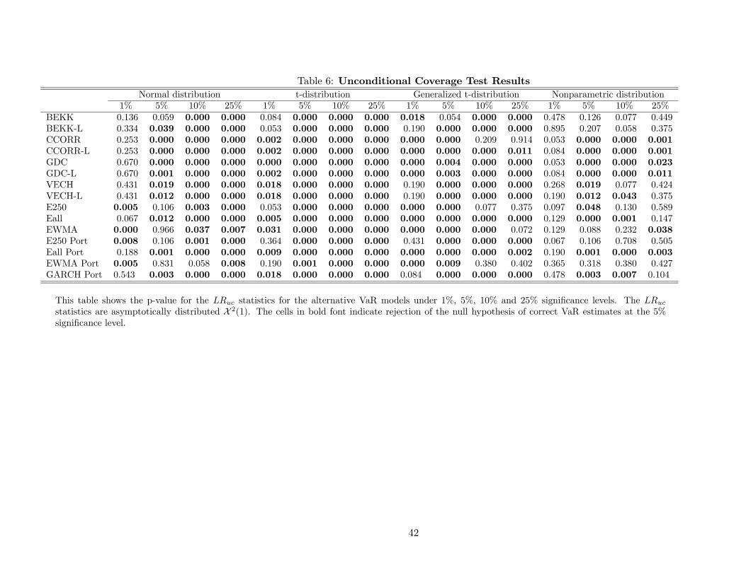
Table 6: Unconditional Coverage Test ResultsNormal distribution t-distribution Generalized t-distribution Nonparametric distribution
1% 5% 10% 25% 1% 5% 10% 25% 1% 5% 10% 25% 1% 5% 10% 25%BEKK 0.136 0.059 0.000 0.000 0.084 0.000 0.000 0.000 0.018 0.054 0.000 0.000 0.478 0.126 0.077 0.449BEKK-L 0.334 0.039 0.000 0.000 0.053 0.000 0.000 0.000 0.190 0.000 0.000 0.000 0.895 0.207 0.058 0.375CCORR 0.253 0.000 0.000 0.000 0.002 0.000 0.000 0.000 0.000 0.000 0.209 0.914 0.053 0.000 0.000 0.001CCORR-L 0.253 0.000 0.000 0.000 0.002 0.000 0.000 0.000 0.000 0.000 0.000 0.011 0.084 0.000 0.000 0.001GDC 0.670 0.000 0.000 0.000 0.000 0.000 0.000 0.000 0.000 0.004 0.000 0.000 0.053 0.000 0.000 0.023GDC-L 0.670 0.001 0.000 0.000 0.002 0.000 0.000 0.000 0.000 0.003 0.000 0.000 0.084 0.000 0.000 0.011VECH 0.431 0.019 0.000 0.000 0.018 0.000 0.000 0.000 0.190 0.000 0.000 0.000 0.268 0.019 0.077 0.424VECH-L 0.431 0.012 0.000 0.000 0.018 0.000 0.000 0.000 0.190 0.000 0.000 0.000 0.190 0.012 0.043 0.375E250 0.005 0.106 0.003 0.000 0.053 0.000 0.000 0.000 0.000 0.000 0.077 0.375 0.097 0.048 0.130 0.589Eall 0.067 0.012 0.000 0.000 0.005 0.000 0.000 0.000 0.000 0.000 0.000 0.000 0.129 0.000 0.001 0.147EWMA 0.000 0.966 0.037 0.007 0.031 0.000 0.000 0.000 0.000 0.000 0.000 0.072 0.129 0.088 0.232 0.038E250 Port 0.008 0.106 0.001 0.000 0.364 0.000 0.000 0.000 0.431 0.000 0.000 0.000 0.067 0.106 0.708 0.505Eall Port 0.188 0.001 0.000 0.000 0.009 0.000 0.000 0.000 0.000 0.000 0.000 0.002 0.190 0.001 0.000 0.003EWMA Port 0.005 0.831 0.058 0.008 0.190 0.001 0.000 0.000 0.000 0.009 0.380 0.402 0.365 0.318 0.380 0.427GARCH Port 0.543 0.003 0.000 0.000 0.018 0.000 0.000 0.000 0.084 0.000 0.000 0.000 0.478 0.003 0.007 0.104
This table shows the p-value for the LRuc statistics for the alternative VaR models under 1%, 5%, 10% and 25% significance levels. The LRucstatistics are asymptotically distributed X 2(1). The cells in bold font indicate rejection of the null hypothesis of correct VaR estimates at the 5%significance level.
42

Table 7: Conditional Coverage Test ResultsNormal distribution t-distribution Generalized t-distribution nonparametric distribution
1% 5% 10% 25% 1% 5% 10% 25% 1% 5% 10% 25% 1% 5% 10% 25%BEKK 0.203 0.082 0.000 0.000 0.196 0.000 0.000 0.000 0.054 0.000 0.000 0.000 0.625 0.183 0.074 0.692BEKK-L 0.416 0.081 0.000 0.000 0.135 0.000 0.000 0.000 0.358 0.000 0.000 0.000 0.753 0.300 0.051 0.609CCORR 0.337 0.000 0.000 0.000 0.009 0.000 0.000 0.000 0.000 0.000 0.142 0.992 0.135 0.000 0.000 0.003CCORR-L 0.337 0.000 0.000 0.000 0.009 0.000 0.000 0.000 0.000 0.000 0.000 0.040 0.196 0.000 0.000 0.004GDC 0.650 0.001 0.000 0.000 0.002 0.000 0.000 0.000 0.001 0.002 0.000 0.000 0.135 0.000 0.000 0.075GDC-L 0.650 0.002 0.000 0.000 0.009 0.000 0.000 0.000 0.002 0.002 0.000 0.000 0.196 0.000 0.000 0.040VECH 0.499 0.040 0.000 0.000 0.054 0.000 0.000 0.000 0.358 0.000 0.000 0.000 0.450 0.040 0.074 0.732VECH-L 0.499 0.023 0.000 0.000 0.054 0.000 0.000 0.000 0.358 0.000 0.000 0.000 0.358 0.023 0.048 0.681E250 0.008 0.010 0.000 0.000 0.135 0.000 0.000 0.000 0.000 0.000 0.015 0.528 0.206 0.008 0.022 0.735Eall 0.109 0.000 0.000 0.000 0.017 0.000 0.000 0.000 0.000 0.000 0.000 0.000 0.272 0.000 0.001 0.338EWMA 0.001 0.384 0.053 0.028 0.088 0.000 0.000 0.000 0.000 0.000 0.000 0.201 0.272 0.125 0.279 0.110E250 Port 0.027 0.010 0.000 0.000 0.542 0.000 0.000 0.000 0.511 0.000 0.000 0.000 0.157 0.010 0.065 0.784Eall Port 0.265 0.000 0.000 0.000 0.031 0.000 0.000 0.000 0.000 0.000 0.000 0.005 0.359 0.000 0.000 0.012EWMA Port 0.018 0.421 0.091 0.032 0.358 0.002 0.000 0.000 0.000 0.010 0.389 0.688 0.542 0.186 0.389 0.706GARCH Port 0.579 0.005 0.000 0.000 0.054 0.000 0.000 0.000 0.196 0.000 0.000 0.000 0.625 0.005 0.006 0.266
This table shows the p-value for the LRcc statistics for the alternative VaR models under 1%, 5%, 10% and 25% significance levels. The LRcc statisticsare asymptotically distributed X 2(2). The cells in bold font indicate rejection of the null hypothesis of correct VaR estimates at the 5% significancelevel.
43

Table 8: Dynamic Quantile Test ResultsNormal distribution t-distribution Generalized t-distribution Nonparametric distribution
1% 5% 10% 25% 1% 5% 10% 25% 1% 5% 10% 25% 1% 5% 10% 25%BEKK 0.707 0.090 0.000 0.001 0.522 0.000 0.000 0.000 0.159 0.001 0.000 0.000 0.956 0.111 0.097 0.311BEKK-L 0.877 0.090 0.000 0.000 0.435 0.000 0.000 0.000 0.786 0.000 0.000 0.000 0.959 0.194 0.083 0.323CCORR 0.813 0.000 0.000 0.000 0.006 0.000 0.000 0.000 0.000 0.000 0.515 0.347 0.365 0.000 0.000 0.014CCORR-L 0.813 0.000 0.000 0.000 0.006 0.000 0.000 0.000 0.000 0.000 0.000 0.090 0.485 0.000 0.000 0.020GDC 0.962 0.001 0.000 0.000 0.000 0.000 0.000 0.000 0.000 0.033 0.000 0.000 0.425 0.000 0.002 0.171GDC-L 0.960 0.004 0.000 0.000 0.007 0.000 0.000 0.000 0.000 0.038 0.000 0.000 0.573 0.000 0.001 0.097VECH 0.938 0.067 0.000 0.000 0.154 0.000 0.000 0.000 0.793 0.000 0.000 0.000 0.841 0.067 0.201 0.498VECH-L 0.938 0.068 0.000 0.000 0.153 0.000 0.000 0.000 0.792 0.000 0.000 0.000 0.792 0.068 0.144 0.468E250 0.017 0.000 0.000 0.000 0.145 0.000 0.000 0.000 0.000 0.000 0.000 0.004 0.438 0.000 0.000 0.014Eall 0.213 0.000 0.000 0.000 0.042 0.000 0.000 0.000 0.000 0.000 0.000 0.000 0.383 0.000 0.000 0.333EWMA 0.043 0.104 0.018 0.021 0.173 0.000 0.000 0.000 0.000 0.000 0.000 0.132 0.516 0.013 0.035 0.024E250 Port 0.035 0.000 0.000 0.000 0.832 0.000 0.000 0.000 0.314 0.000 0.000 0.000 0.367 0.000 0.001 0.042Eall Port 0.140 0.000 0.000 0.000 0.066 0.000 0.000 0.000 0.000 0.000 0.000 0.050 0.486 0.000 0.000 0.059EWMA Port 0.053 0.120 0.023 0.023 0.528 0.000 0.000 0.000 0.000 0.000 0.044 0.168 0.772 0.019 0.044 0.135GARCH Port 0.950 0.015 0.000 0.000 0.162 0.000 0.000 0.000 0.572 0.000 0.000 0.000 0.939 0.015 0.039 0.225
This table shows the p-value for the DQ statistic for the alternative VaR models under 1%, 5%, 10% and 25% signficance levels. The DQ statisticsare asymptotically distributed X 2(7). The cells in bold font indicate rejection of the null hypothesis of correct VaR estimates at the 5% significancelevel.
44

Table 9: Distribution Forecast Test ResultsNormal t-distribution Generalized Nonparametric
distribution t-distribution distributionBEKK 0.433 0.000 0.520 0.265BEKK-L 0.329 0.000 0.475 0.381CCORR 0.000 0.000 0.000 0.000CCORR-L 0.000 0.000 0.000 0.000GDC 0.001 0.000 0.016 0.000GDC-L 0.011 0.000 0.041 0.000VECH 0.204 0.000 0.510 0.090VECH-L 0.162 0.000 0.507 0.119E250 0.298 0.000 0.142 0.536Eall 0.160 0.000 0.000 0.000EWMA 0.000 0.000 0.231 0.135E250 Port 0.360 0.000 0.570 0.012Eall Port 0.001 0.000 0.002 0.000EWMA Port 0.000 0.000 0.188 0.804GARCH Port 0.003 0.000 0.035 0.004
This table shows the p-value for the LRdist statistics for the alternative VaR models under 1%, 5%, 10%and 25% quantiles. The LRdist statistic is asymptotically distributed X 2(3). The cells in bold font indicaterejection of the null hypothesis of correct VaR estimates at the 5% significance level.
45
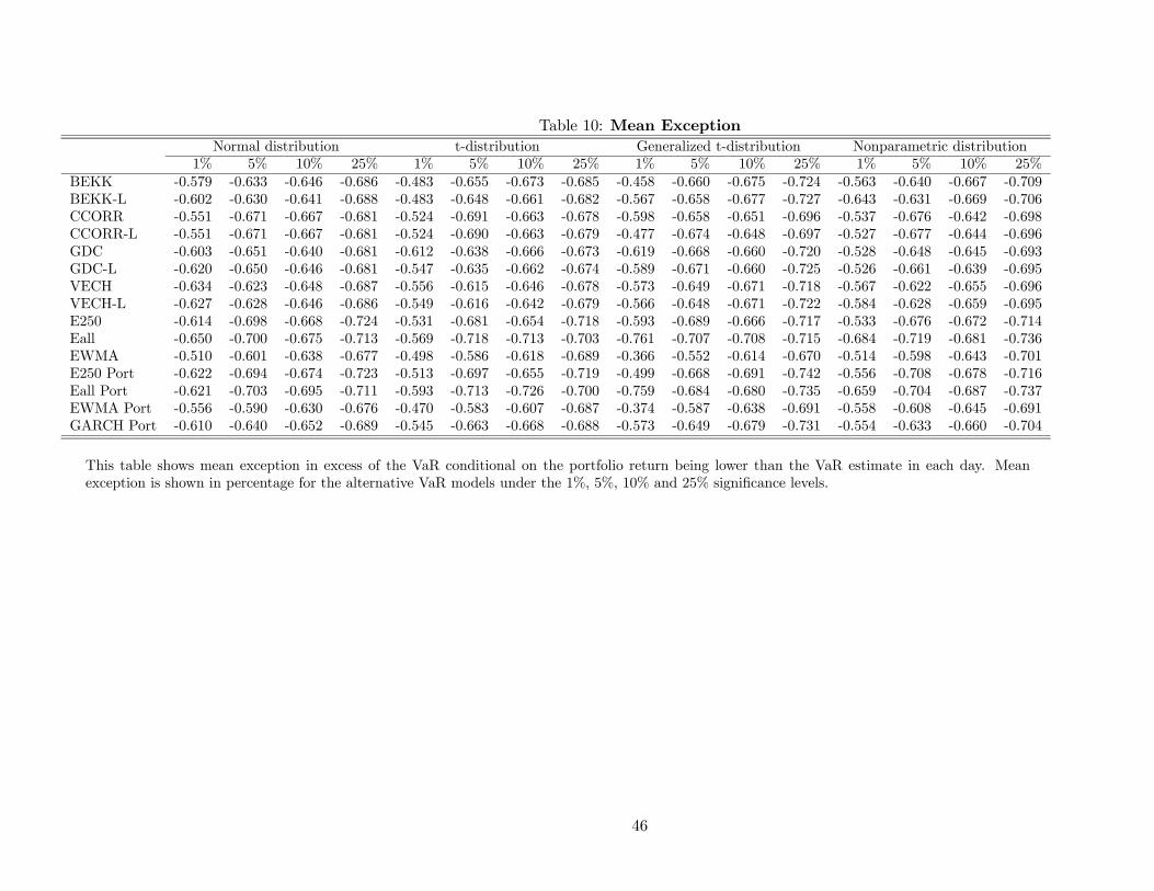
Table 10: Mean ExceptionNormal distribution t-distribution Generalized t-distribution Nonparametric distribution
1% 5% 10% 25% 1% 5% 10% 25% 1% 5% 10% 25% 1% 5% 10% 25%BEKK -0.579 -0.633 -0.646 -0.686 -0.483 -0.655 -0.673 -0.685 -0.458 -0.660 -0.675 -0.724 -0.563 -0.640 -0.667 -0.709BEKK-L -0.602 -0.630 -0.641 -0.688 -0.483 -0.648 -0.661 -0.682 -0.567 -0.658 -0.677 -0.727 -0.643 -0.631 -0.669 -0.706CCORR -0.551 -0.671 -0.667 -0.681 -0.524 -0.691 -0.663 -0.678 -0.598 -0.658 -0.651 -0.696 -0.537 -0.676 -0.642 -0.698CCORR-L -0.551 -0.671 -0.667 -0.681 -0.524 -0.690 -0.663 -0.679 -0.477 -0.674 -0.648 -0.697 -0.527 -0.677 -0.644 -0.696GDC -0.603 -0.651 -0.640 -0.681 -0.612 -0.638 -0.666 -0.673 -0.619 -0.668 -0.660 -0.720 -0.528 -0.648 -0.645 -0.693GDC-L -0.620 -0.650 -0.646 -0.681 -0.547 -0.635 -0.662 -0.674 -0.589 -0.671 -0.660 -0.725 -0.526 -0.661 -0.639 -0.695VECH -0.634 -0.623 -0.648 -0.687 -0.556 -0.615 -0.646 -0.678 -0.573 -0.649 -0.671 -0.718 -0.567 -0.622 -0.655 -0.696VECH-L -0.627 -0.628 -0.646 -0.686 -0.549 -0.616 -0.642 -0.679 -0.566 -0.648 -0.671 -0.722 -0.584 -0.628 -0.659 -0.695E250 -0.614 -0.698 -0.668 -0.724 -0.531 -0.681 -0.654 -0.718 -0.593 -0.689 -0.666 -0.717 -0.533 -0.676 -0.672 -0.714Eall -0.650 -0.700 -0.675 -0.713 -0.569 -0.718 -0.713 -0.703 -0.761 -0.707 -0.708 -0.715 -0.684 -0.719 -0.681 -0.736EWMA -0.510 -0.601 -0.638 -0.677 -0.498 -0.586 -0.618 -0.689 -0.366 -0.552 -0.614 -0.670 -0.514 -0.598 -0.643 -0.701E250 Port -0.622 -0.694 -0.674 -0.723 -0.513 -0.697 -0.655 -0.719 -0.499 -0.668 -0.691 -0.742 -0.556 -0.708 -0.678 -0.716Eall Port -0.621 -0.703 -0.695 -0.711 -0.593 -0.713 -0.726 -0.700 -0.759 -0.684 -0.680 -0.735 -0.659 -0.704 -0.687 -0.737EWMA Port -0.556 -0.590 -0.630 -0.676 -0.470 -0.583 -0.607 -0.687 -0.374 -0.587 -0.638 -0.691 -0.558 -0.608 -0.645 -0.691GARCH Port -0.610 -0.640 -0.652 -0.689 -0.545 -0.663 -0.668 -0.688 -0.573 -0.649 -0.679 -0.731 -0.554 -0.633 -0.660 -0.704
This table shows mean exception in excess of the VaR conditional on the portfolio return being lower than the VaR estimate in each day. Meanexception is shown in percentage for the alternative VaR models under the 1%, 5%, 10% and 25% significance levels.
46
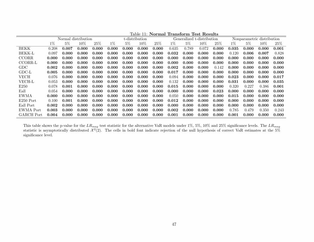
Table 11: Normal Transform Test ResultsNormal distribution t-distribution Generalized t-distribution Nonparametric distribution
1% 5% 10% 25% 1% 5% 10% 25% 1% 5% 10% 25% 1% 5% 10% 25%BEKK 0.208 0.007 0.000 0.000 0.000 0.000 0.000 0.000 0.635 0.789 0.072 0.000 0.035 0.000 0.000 0.001BEKK-L 0.097 0.000 0.000 0.000 0.000 0.000 0.000 0.000 0.032 0.000 0.000 0.000 0.120 0.006 0.007 0.828CCORR 0.000 0.000 0.000 0.000 0.000 0.000 0.000 0.000 0.000 0.000 0.000 0.000 0.000 0.000 0.000 0.000CCORR-L 0.000 0.000 0.000 0.000 0.000 0.000 0.000 0.000 0.000 0.000 0.000 0.000 0.000 0.000 0.000 0.000GDC 0.002 0.000 0.000 0.000 0.000 0.000 0.000 0.000 0.002 0.000 0.000 0.142 0.000 0.000 0.000 0.000GDC-L 0.005 0.000 0.000 0.000 0.000 0.000 0.000 0.000 0.017 0.000 0.000 0.000 0.000 0.000 0.000 0.000VECH 0.076 0.000 0.000 0.000 0.000 0.000 0.000 0.000 0.094 0.000 0.000 0.000 0.023 0.000 0.000 0.017VECH-L 0.053 0.000 0.000 0.000 0.000 0.000 0.000 0.000 0.132 0.000 0.000 0.000 0.031 0.000 0.000 0.035E250 0.078 0.001 0.000 0.000 0.000 0.000 0.000 0.000 0.015 0.000 0.000 0.000 0.320 0.227 0.386 0.001Eall 0.054 0.000 0.000 0.000 0.000 0.000 0.000 0.000 0.000 0.000 0.000 0.023 0.000 0.000 0.000 0.000EWMA 0.000 0.000 0.000 0.000 0.000 0.000 0.000 0.000 0.050 0.000 0.000 0.000 0.015 0.000 0.000 0.000E250 Port 0.100 0.001 0.000 0.000 0.000 0.000 0.000 0.000 0.012 0.000 0.000 0.000 0.000 0.000 0.000 0.000Eall Port 0.002 0.000 0.000 0.000 0.000 0.000 0.000 0.000 0.000 0.000 0.000 0.000 0.000 0.000 0.000 0.000EWMA Port 0.003 0.000 0.000 0.000 0.000 0.000 0.000 0.000 0.002 0.000 0.000 0.000 0.785 0.479 0.350 0.243GARCH Port 0.004 0.000 0.000 0.000 0.000 0.000 0.000 0.000 0.001 0.000 0.000 0.000 0.001 0.000 0.000 0.000
This table shows the p-value for the LRmag test statistic for the alternative VaR models under 1%, 5%, 10% and 25% significance levels. The LRmagstatistic is asymptotically distributed X 2(2). The cells in bold font indicate rejection of the null hypothesis of correct VaR estimates at the 5%significance level.
47

Table 12: Capital Charge Relative to Benchmark Model - EWMA-NormalNormal distrib. t-distribution Generalized t-distrib. Nonparametric distrib.
% trading p-value % trading p-value % trading p-value % trading p-valueBEKK 57.11 0.539 87.14 0.000 89.66 0.000 70.43 0.010BEKK-L 55.40 0.696 87.33 0.000 78.14 0.000 58.34 0.246CCORR 67.45 0.010 92.52 0.000 98.89 0.000 87.29 0.000CCORR-L 67.45 0.010 92.56 0.000 100.00 0.000 87.03 0.000GDC 60.70 0.072 93.78 0.000 93.82 0.000 83.29 0.000GDC-L 60.02 0.140 92.98 0.000 93.86 0.000 81.34 0.000VECH 61.92 0.221 90.11 0.000 80.20 0.000 77.34 0.000VECH-L 63.37 0.168 90.35 0.000 81.19 0.000 78.79 0.000E250 58.64 0.256 79.55 0.000 97.48 0.000 67.65 0.028Eall 65.01 0.211 84.74 0.000 97.60 0.000 71.96 0.010EWMA - - 99.35 0.000 100.00 0.000 92.56 0.000E250 Port 57.76 0.240 77.45 0.000 70.89 0.000 65.82 0.050Eall Port 68.45 0.123 83.94 0.000 94.35 0.000 71.92 0.012EWMA Port 36.28 0.996 93.02 0.000 100.00 0.000 82.07 0.000GARCH Port 61.92 0.165 86.91 0.000 80.24 0.000 77.30 0.000
This table shows the percentage of trading days for which the benchmark VaR model (EWMA-Normal)has lower capital charge than the one given by the each model. The cells in bold font indicate rejectionof the null hypothesis of equal capital charges at the 5% significance level using the Diebold-Mariano teststatistic.
48

Table 13: Capital Charge Relative to Benchmark Model - EWMA Portfolio-NormalNormal distrib. t-distrib. Generalized t-distrib. Nonparametric distrib.
% trading p-value % trading p-value % trading p-value % trading p-valueBEKK 66.34 0.039 96.49 0.000 96.22 0.000 76.50 0.000BEKK-L 63.56 0.087 94.20 0.000 86.99 0.000 69.29 0.003CCORR 75.93 0.000 95.23 0.000 100.00 0.000 95.77 0.000CCORR-L 75.96 0.000 95.23 0.000 100.00 0.000 95.42 0.000GDC 73.03 0.000 96.11 0.000 96.30 0.000 90.92 0.000GDC-L 71.96 0.001 96.07 0.000 96.22 0.000 90.23 0.000VECH 71.30 0.001 95.80 0.000 90.42 0.000 87.52 0.000VECH-L 72.15 0.001 95.84 0.000 91.11 0.000 88.33 0.000E250 63.41 0.074 82.49 0.000 98.55 0.000 71.65 0.003Eall 68.49 0.054 88.36 0.000 99.73 0.000 75.43 0.001EWMA 63.72 0.004 100.00 0.000 100.00 0.000 99.85 0.000E250 Port 62.99 0.066 80.69 0.000 74.21 0.000 70.16 0.007Eall Port 71.69 0.025 86.88 0.000 96.80 0.000 75.39 0.001EWMA Port - - 99.85 0.000 100.00 0.000 93.82 0.000GARCH Port 70.89 0.003 92.60 0.000 86.53 0.000 84.59 0.000
This table shows the percentage of trading days for which the benchmark VaR model (EWMA—PortfolioNormal) has lower capital charge than the one given by the each model. The cells in bold fontindicate rejection of the null hypothesis of equal capital charges at the 5% significance level using theDiebold-Mariano test statistic.
49