Evaluating LTL Satisfiability Solvers

Viktor Schuppan1 and Luthfi Darmawan2

1 Email: Viktor.Schuppan@gmx.de2 Email: luthfi@alumni.itb.ac.id

Abstract. We perform a comprehensive experimental evaluation of off-the-shelf solvers for satisfiability of propositional LTL. We consider awide range of solvers implementing three major classes of algorithms:reduction to model checking, tableau-based approaches, and temporalresolution. Our set of benchmark families is significantly more compre-hensive than those in previous studies. It takes the benchmark families ofprevious studies, which only have a limited overlap, and adds benchmarkfamilies not used for that purpose before.We find that no solver dominates or solves all instances. Solvers focusedon finding models and solvers using temporal resolution or fixed pointcomputation show complementary strengths and weaknesses. This moti-vates and guides estimation of the potential of a portfolio solver. It turnsout that even combining two solvers in a simple fashion significantly in-creases the share of solved instances while reducing CPU time spent.

1 Introduction

More and more, system specifications are not only used for classical verificationof the correctness of a given system, e.g., via model checking, but they themselvesbecome the subject of investigation (e.g., [56,33]). This is justified by observa-tions in industry that many specifications contain errors (e.g., [16]) as well as bytransition to property-based design (e.g., [57]). Propositional Linear TemporalLogic (LTL) [29] is a popular choice for system specifications and many checkson specifications reduce to determining (un)satisfiability (see, e.g., [56,33,60]).Hence, satisfiability of LTL is of considerable practical relevance.

A broad range of techniques for determining satisfiability of LTL has beendeveloped: tableau-based methods (e.g., [68,48,63]), temporal resolution (e.g.,[32]), and reduction to model checking (e.g., [60,69,25]). Despite the relevanceof the problem and the range of techniques, we are not aware of a recent, com-prehensive experimental comparison of solvers for satisfiability of propositionalLTL on a broad set of benchmarks. In fact, the only line of work containing arepresentative from each of the above mentioned techniques that we know is theone by Hustadt et al. [45,42,46] (see below), which is somewhat dated.

In this paper we make the following contributions. 1. We perform an experi-mental evaluation of solvers for satisfiability of propositional LTL using ALASKA

[1,69], LWB [2,41], NuSMV [3,26], pltl [4], TRP++ [5,44], and TSPASS [6,51]. Boththe range of techniques in the solvers we use and the set of benchmarks we col-lected are significantly more comprehensive than in any previous study we know.

We have made our data available for further analysis [7]. 2. We consider num-ber of solved instances, run time, memory usage, and model size. The analysisis greatly helped by using contour/discrete raw data plots, which complementthe traditional cactus plots by preserving the relationship between benchmarkinstances. 3. The analysis shows complementary behavior between some solvers.This motivates estimating the potential of a portfolio solver. We consider port-folio solvers without communication between members of the portfolio for a bestcase scenario (which is unrealistic) and a reference case scenario (which anyportfolio solver should aim to beat). Finally, we show that even a trivially im-plementable solver that sequentially executes one solver first for a short amountof time and, if necessary, then invokes another solver reduces the number ofunsolved instances as well as the average run time.

Related Work Rozier and Vardi compare several explicit state and symbolicBDD-based model checkers for LTL satisfiability checking [60]. They find thesymbolic tools to be superior in terms of performance and, generally, also interms of quality. They do not consider SAT-based bounded model checkers,tableau-based solvers, or temporal resolution. While they perform an in-depthcomparison of solvers using very similar techniques, our focus is on comparingselected representatives of a broad variety of techniques. We also use more bench-mark families and consider memory usage and model size. The same authorscompare symbolic constructions of Buchi automata in [59] using the BDD-basedengine of Cadence SMV as backend solver. They show that a portfolio approachto automata construction is advantageous. De Wulf et al. compare NuSMV andALASKA [69]. For a detailed discussion see Sect. 6. Hustadt et al. perform severalcomparisons [45,42,46] of TRP, a version of LWB, and a version of SMV on the trpbenchmark set (see Sect. 4). Gore and Widmann perform an experimental com-parison of solvers for CTL [37]. Goranko et al. [35] compare an implementation ofWolper’s tableau construction with pltl. For references on solver competitionsand on their methodology see App. A of [62].

We are not aware of previous work on portfolio approaches to LTL satisfi-ability, except for [59]. We use entire solvers as members of a portfolio, while[59] uses different frontends for Buchi automata construction all relying on thesame BDD-based backend solver. For other problem classes see, e.g., [43] (graphcoloring, web browsing), [49] (winner determination problem), [34] (constraintsatisfaction, mixed integer programming), [70] (SAT), or [58] (QBF).

Organization In Sect. 2 we introduce notation. In Sect. 3, 4, and 5 we de-scribe solvers, benchmarks, and methodology. Section 6 contains the results ofour evaluation. An estimation of the potential of a portfolio solver follows inSect. 7. Section 8 concludes. Due to space constraints the following parts arein appendices [62]: general concepts and terminology (App. A), details on ourbenchmark set (App. B), discussion (App. C), and some plots (App. D).

2 Preliminaries

We consider formulas in future time propositional LTL with temporal operatorsF, G, R, U, X. We assume familiarity with LTL; otherwise see [29].

2

The terminology we use is largely standard (e.g., [64,19]); a reader unfa-miliar with competition terminology is referred to App. A of [62]. A somewhatnon-standard term we use is configuration, which denotes a tool (solver) withspecific option values. A tool is a state-of-the-art contributor (sota) if an instanceis solved only by configurations of that tool (see also [66]). Given a set of config-urations C the virtual best solver (vbs) is the hypothetical solver using the bestconfiguration in C on any given instance (e.g., [19]). We use bold font for setsof benchmark instances and teletype for configurations.

3 Solvers

Choice of Solvers We consider tools to solve satisfiability of propositional LTLfrom 3 major classes of approaches: 1. reduction to model checking, 2. tableau-based algorithms, and 3. temporal resolution. Tools were chosen as detailedbelow. To the best of our knowledge this set of solvers is the most diverse con-sidered in an evaluation of solvers for satisfiability of propositional LTL to date.

Reduction to Model Checking We chose ALASKA [1,69] and NuSMV [3,26] usingBDDs (NuSMV-BDD) and SAT (NuSMV-SBMC). We ruled out explicit state modelcheckers, as they did not scale as well as BDD-based symbolic model checkersfor LTL satisfiability in [60]. The BDD-based engine of Cadence SMV [8] per-formed comparable to NuSMV-BDD in [60]. sal-smc [54] constructs explicit Buchiautomata and was found not to scale [60]. The BDD-based variant of VIS [67]uses explicit construction of Buchi automata; initial experiments confirmed thatthis does not scale for satisfiability of LTL. sal-bmc [54] can only prove safetyproperties [53]. For an alternative using SAT-based symbolic model checking wecontacted the VIS group for advice on recommended configurations (the spaceof configurations is quite large), but have not received an answer yet. Finally, wechecked the publicly available versions of the participants of HWMCC’10 [20];as far as we could see, the solvers that are not included in our study only handlesafety properties.

Tableau-Based Algorithms We chose LWB [2,41] and pltl [4]. TWB [15] is super-seded by pltl [36]. LTL Tableau turns out to be inferior to pltl [35].

Temporal Resolution We chose TRP++ [5,44] and TSPASS [6,51]. An alternativetool is TeMP [47]. TeMP was shown to be inferior to TRP++ on propositional prob-lems in [47] and comparable to TSPASS on monodic problems in [51]. Note, thatTSPASS is fair, while TeMP is not [50].

Solver Descriptions Below we briefly describe the tools we consider as well asthe set of their options that we take into account. Note that not all combinationsof options are valid. Due to space constraints the descriptions have to be keptshort, and we refer the reader to the respective tool documentation.

ALASKA performs model checking and satisfiability checking of LTL via symboliccomputation of fixed points using antichains [1,69]. Relevant options are: noc/cdis-/enables model construction, nos/s uses a semisymbolic/fully symbolic algo-rithm, and nob/b switches between forward and backward image computation.We use version 0.4 with an additional patch by N. Maquet.

3

LWB [2,41] implements tableau-based algorithms for LTL by Janssen [48] (nomodel construction) in the function “satisfiable” and by Schwendimann [63](model construction) in the function “model”. Neither has relevant options. Wedesignate the former by sat and the latter by mod. We use version 1.1.

NuSMV-BDD In this evaluation we treat NuSMV [3,26] as two tools NuSMV-BDD

and NuSMV-SBMC. NuSMV-BDD performs symbolic model checking of LTL usingsymbolic fixed point computation with BDDs [27]. Experience with NuSMV-BDD

allows us to restrict experiments to the following options. nodcx/dcx en-/disablesmodel construction, nofflt/fflt dis-/enables forward computation of reachablestates in the model and tableau for the LTL formula, nodyn/dyn dis-/enablesdynamic reordering, and elbwd/elfwd switches between backward and forwardimage computation in the Emerson-Lei algorithm [30,40]. We use version 2.5.0.

NuSMV-SBMC performs incremental simple bounded model checking [39] of LTLusing MiniSat [9]. Options considered are nodcx/dcx to en-/disable model con-struction and noc/c to dis-/enable checking completeness. With the latter dis-abled NuSMV-SBMC cannot solve unsat instances. We use version 2.5.0.

pltl [4] implements tableau-based algorithms for LTL along the lines of [38] viathe command line argument “graph” and by Schwendimann [63] via the com-mand line argument “tree”. Neither has model construction or relevant options.We designate the former by graph and the latter by tree. We use version r1424.

TRP++ [5,44] uses temporal resolution for LTL [32]. Relevant options: nos/sto dis-/enable simplification, nor/r to dis-/enable rewriting, noal/al to ex-/include an order statement, dfs/bfs to choose dfs/bfs in loop search, nop/pto dis-/enable pre-test for sometime resolution, and nofsr/fsr to dis-/enableforward subsumption resolution. TRP++ cannot construct models. We use v. 2.x.

TSPASS [6,51] is a temporal resolution solver for monodic first-order temporallogic with model construction for propositional LTL [52]. We consider noext/extto dis-/enable extended step clauses, nogrp/grp to dis-/enable regrouping of X,nosev/sev to dis-/enable transforming multiple eventualities into a single one,log/sub to select logical equivalence or subsumption in loop tests, nosls/sls todis-/enable sequential loop search, norfmrr/rfmrr (resp. norbmrr/rbmrr) to dis-/enable forward (resp. backward) matching replacement resolution, nomod/modto dis-/enable model construction, and mur/mor to select unordered or orderedresolution in model construction. We use version 0.94-0.16.

4 Benchmarks

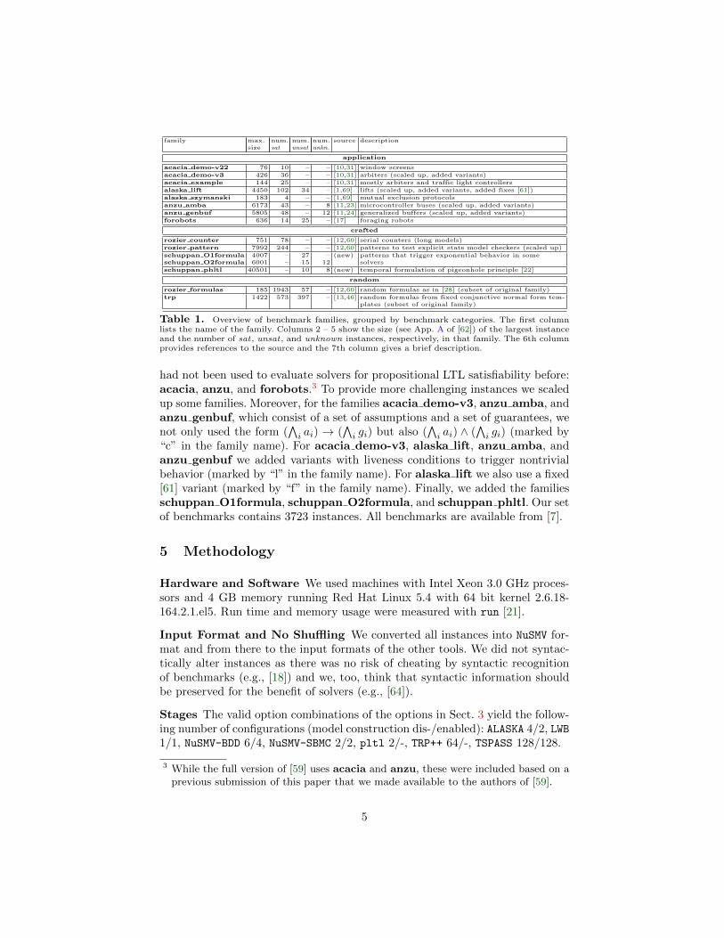
In Tab. 1 we give an overview of the benchmark families we use. Toour knowledge this set of benchmarks is the most comprehensive usedfor evaluating propositional LTL satisfiability solvers so far. [60] usedrozier counter, rozier pattern, and rozier formulas. [69] used alaska lift,alaska szymanski, and subsets of rozier counter and rozier formulas. [46]used trp. Note that there is little overlap. [60,69] and [46] represent separate com-munities. We added the following benchmark families that, to our knowledge,

4

family max. num. num. num. source descriptionsize sat unsat unkn.

application

acacia demo-v22 76 10 – – [10,31] window screens

acacia demo-v3 426 36 – – [10,31] arbiters (scaled up, added variants)

acacia example 144 25 – – [10,31] mostly arbiters and traffic light controllers

alaska lift 4450 102 34 – [1,69] lifts (scaled up, added variants, added fixes [61])

alaska szymanski 183 4 – – [1,69] mutual exclusion protocols

anzu amba 6173 43 – 8 [11,23] microcontroller buses (scaled up, added variants)

anzu genbuf 5805 48 – 12 [11,24] generalized buffers (scaled up, added variants)

forobots 636 14 25 – [17] foraging robots

crafted

rozier counter 751 78 – – [12,60] serial counters (long models)

rozier pattern 7992 244 – – [12,60] patterns to test explicit state model checkers (scaled up)

schuppan O1formula 4007 – 27 – (new) patterns that trigger exponential behavior in someschuppan O2formula 6001 – 15 12 solvers

schuppan phltl 40501 – 10 8 (new) temporal formulation of pigeonhole principle [22]

random

rozier formulas 185 1943 57 – [12,60] random formulas as in [28] (subset of original family)

trp 1422 573 397 – [13,46] random formulas from fixed conjunctive normal form tem-plates (subset of original family)

Table 1. Overview of benchmark families, grouped by benchmark categories. The first columnlists the name of the family. Columns 2 – 5 show the size (see App. A of [62]) of the largest instanceand the number of sat, unsat, and unknown instances, respectively, in that family. The 6th columnprovides references to the source and the 7th column gives a brief description.

had not been used to evaluate solvers for propositional LTL satisfiability before:acacia, anzu, and forobots.3 To provide more challenging instances we scaledup some families. Moreover, for the families acacia demo-v3, anzu amba, andanzu genbuf, which consist of a set of assumptions and a set of guarantees, wenot only used the form (

∧i ai) → (

∧i gi) but also (

∧i ai) ∧ (

∧i gi) (marked by

“c” in the family name). For acacia demo-v3, alaska lift, anzu amba, andanzu genbuf we added variants with liveness conditions to trigger nontrivialbehavior (marked by “l” in the family name). For alaska lift we also use a fixed[61] variant (marked by “f” in the family name). Finally, we added the familiesschuppan O1formula, schuppan O2formula, and schuppan phltl. Our setof benchmarks contains 3723 instances. All benchmarks are available from [7].

5 Methodology

Hardware and Software We used machines with Intel Xeon 3.0 GHz proces-sors and 4 GB memory running Red Hat Linux 5.4 with 64 bit kernel 2.6.18-164.2.1.el5. Run time and memory usage were measured with run [21].

Input Format and No Shuffling We converted all instances into NuSMV for-mat and from there to the input formats of the other tools. We did not syntac-tically alter instances as there was no risk of cheating by syntactic recognitionof benchmarks (e.g., [18]) and we, too, think that syntactic information shouldbe preserved for the benefit of solvers (e.g., [64]).

Stages The valid option combinations of the options in Sect. 3 yield the follow-ing number of configurations (model construction dis-/enabled): ALASKA 4/2, LWB1/1, NuSMV-BDD 6/4, NuSMV-SBMC 2/2, pltl 2/-, TRP++ 64/-, TSPASS 128/128.

3 While the full version of [59] uses acacia and anzu, these were included based on aprevious submission of this paper that we made available to the authors of [59].

5

The number of configurations of TRP++ and TSPASS is too large to includeall of them in the main stage of our evaluation. We therefore performed a pre-liminary stage with a time limit of 10 seconds and a memory limit of 2 GB ona representative subset of instances. In that stage we used all 64 combinationsof TRP++. For TSPASS we considered the following subset of configurations: alloptions at their default value (sometimes implied by other options) as well asa single option switched to its non-default value. This resulted in 24/24 con-figurations. We then fixed options that either had a clear benefit one way orthe other or clearly had little effect to the corresponding values and kept theremaining configurations for the main stage (see Sect. 6). In the main stage allconfigurations of ALASKA, LWB, NuSMV-BDD, NuSMV-SBMC, and pltl as well as theremaining configurations of TRP++ and TSPASS were run with a time limit of 60seconds and a memory limit of 2 GB.

In each stage, each configuration was run only once on each instance. Whileperforming more than one run would provide more accurate information aboutrun time distributions [55] performing only a single run allows to use moreconfigurations, more instances, or higher time bounds with equal resources.

Tracks We have two tracks: one for configurations with model construction dis-or enabled (e.g., LWB using mod constructs models but is superior to sat thatdoesn’t) and one for configurations with model construction enabled. The formerconsiders all instances; the latter is restricted to sat instances.

Correctness of Solvers is a recurring issue in tool competitions and com-parisons (e.g., [60]). Besides obvious cross checking of the sat/unsat results re-ported by different configurations for the same instance we used the fact thatNuSMV-SBMC produces shortest (possibly plus one) models as an additional cor-rectness check. We did not perform further validation of generated models.

Scoring We essentially use scoring based on a higher number of solved instancesand lower time taken on solved instances (see Sect. 2) as it preserves and clearlyshows what we consider two important performance indicators.

However, there are fairly big differences in the number of instances in ourbenchmark families. Still, we would like to consider many benchmarks ratherthan only sampling the larger families. Hence, we modify the above scoringmethod as follows. We consider the benchmark families as a tree. We then com-pute the share of solved instances and the average run time on solved instancesfor each leaf (here all instances have equal weight). Then, for each non-leaf node,aggregate values are computed as averages with equal weights for all children ofthat node. For the tree of families see App. B.2 of [62].

6 Results

For more plots and data see App. D of the full version [62] and the website [7].

Preliminary Stage For TRP++ configurations with s nor proved inferior so thatonly s r, nos r, and nos nor were kept. The effects of noal/al, dfs/bfs, andnofsr/fsr are unclear; hence all combinations were kept. nop/p had little effectso that we set it to its default nop. All in all this left us with 24 configurations.

6

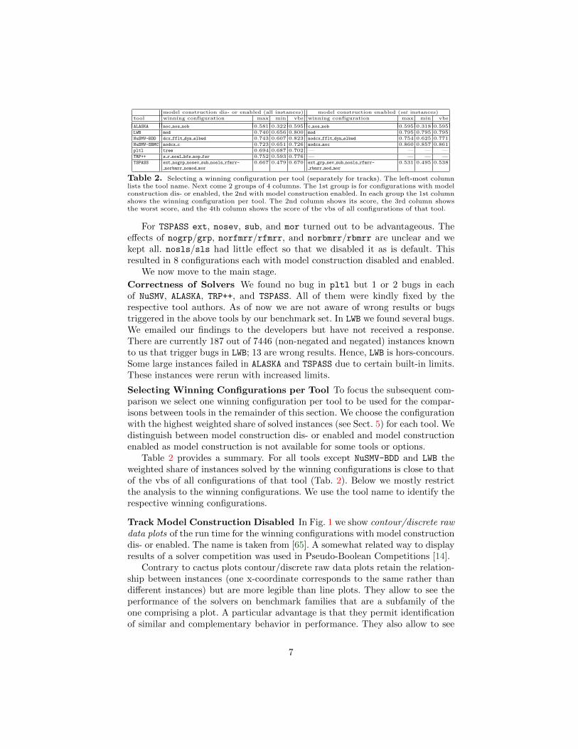
model construction dis- or enabled (all instances) model construction enabled (sat instances)

tool winning configuration max min vbs winning configuration max min vbs

ALASKA noc nos nob 0.581 0.322 0.595 c nos nob 0.595 0.318 0.595

LWB mod 0.740 0.656 0.800 mod 0.795 0.795 0.795

NuSMV-BDD dcx fflt dyn elbwd 0.743 0.607 0.823 nodcx fflt dyn elbwd 0.754 0.625 0.771

NuSMV-SBMC nodcx c 0.723 0.651 0.726 nodcx noc 0.860 0.857 0.861

pltl tree 0.694 0.687 0.702 — — — —

TRP++ s r noal bfs nop fsr 0.752 0.593 0.776 — — — —

TSPASS ext nogrp nosev sub nosls rfmrr-

norbmrr nomod mor

0.667 0.479 0.670 ext grp sev sub nosls rfmrr-

rbmrr mod mor

0.531 0.495 0.538

Table 2. Selecting a winning configuration per tool (separately for tracks). The left-most columnlists the tool name. Next come 2 groups of 4 columns. The 1st group is for configurations with modelconstruction dis- or enabled, the 2nd with model construction enabled. In each group the 1st columnshows the winning configuration per tool. The 2nd column shows its score, the 3rd column showsthe worst score, and the 4th column shows the score of the vbs of all configurations of that tool.

For TSPASS ext, nosev, sub, and mor turned out to be advantageous. Theeffects of nogrp/grp, norfmrr/rfmrr, and norbmrr/rbmrr are unclear and wekept all. nosls/sls had little effect so that we disabled it as is default. Thisresulted in 8 configurations each with model construction disabled and enabled.

We now move to the main stage.

Correctness of Solvers We found no bug in pltl but 1 or 2 bugs in eachof NuSMV, ALASKA, TRP++, and TSPASS. All of them were kindly fixed by therespective tool authors. As of now we are not aware of wrong results or bugstriggered in the above tools by our benchmark set. In LWB we found several bugs.We emailed our findings to the developers but have not received a response.There are currently 187 out of 7446 (non-negated and negated) instances knownto us that trigger bugs in LWB; 13 are wrong results. Hence, LWB is hors-concours.Some large instances failed in ALASKA and TSPASS due to certain built-in limits.These instances were rerun with increased limits.

Selecting Winning Configurations per Tool To focus the subsequent com-parison we select one winning configuration per tool to be used for the compar-isons between tools in the remainder of this section. We choose the configurationwith the highest weighted share of solved instances (see Sect. 5) for each tool. Wedistinguish between model construction dis- or enabled and model constructionenabled as model construction is not available for some tools or options.

Table 2 provides a summary. For all tools except NuSMV-BDD and LWB theweighted share of instances solved by the winning configurations is close to thatof the vbs of all configurations of that tool (Tab. 2). Below we mostly restrictthe analysis to the winning configurations. We use the tool name to identify therespective winning configurations.

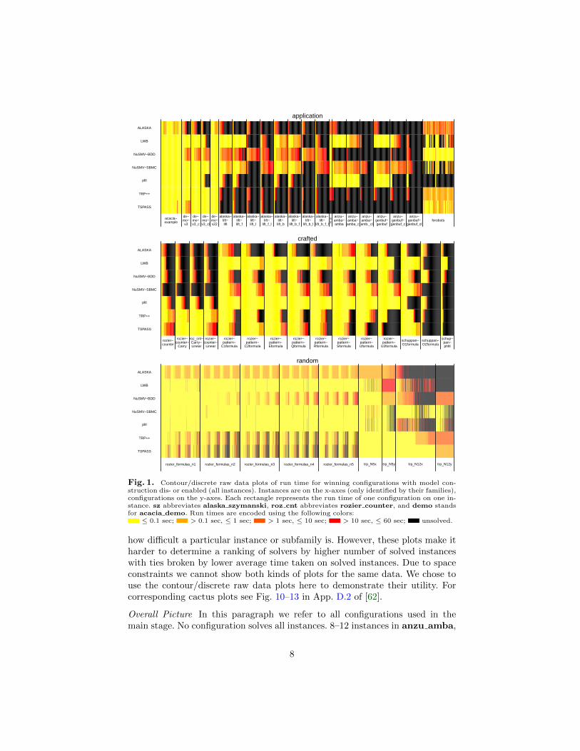
Track Model Construction Disabled In Fig. 1 we show contour/discrete rawdata plots of the run time for the winning configurations with model constructiondis- or enabled. The name is taken from [65]. A somewhat related way to displayresults of a solver competition was used in Pseudo-Boolean Competitions [14].

Contrary to cactus plots contour/discrete raw data plots retain the relation-ship between instances (one x-coordinate corresponds to the same rather thandifferent instances) but are more legible than line plots. They allow to see theperformance of the solvers on benchmark families that are a subfamily of theone comprising a plot. A particular advantage is that they permit identificationof similar and complementary behavior in performance. They also allow to see

7

acacia−example

de−mo−v3

de−mo−v3_c

de−mo−v3_cl

de−mo−v22

alaska−lift−lift

alaska−lift−lift_f

alaska−lift−lift_l

alaska−lift−

lift_f_l

alaska−lift−lift_b

alaska−lift−

lift_b_f

alaska−lift−

lift_b_l

alaska−lift−

lift_b_f_l

sz

anzu−amba−amba

anzu−amba−amba_c

anzu−amba−amb._cl

anzu−genbuf−genbuf

anzu−genbuf−genbuf_c

anzu−genbuf−

genbuf_clforobots

TSPASS

TRP++

pltl

NuSMV−SBMC

NuSMV−BDD

LWB

ALASKA

application

rozier−counter

rozier−counter−

Carry

roz_cnt−Carry−Linear

rozier−counter−

Linear

rozier−pattern−

C1formula

rozier−pattern−

C2formula

rozier−pattern−Eformula

rozier−pattern−Qformula

rozier−pattern−Rformula

rozier−pattern−Sformula

rozier−pattern−Uformula

rozier−pattern−

U2formula

schuppan−O1formula

schuppan−O2formula

schup−pan−phltl

TSPASS

TRP++

pltl

NuSMV−SBMC

NuSMV−BDD

LWB

ALASKA

crafted

rozier_formulas_n1 rozier_formulas_n2 rozier_formulas_n3 rozier_formulas_n4 rozier_formulas_n5 trp_N5x trp_N5y trp_N12x trp_N12y

TSPASS

TRP++

pltl

NuSMV−SBMC

NuSMV−BDD

LWB

ALASKA

random

Fig. 1. Contour/discrete raw data plots of run time for winning configurations with model con-struction dis- or enabled (all instances). Instances are on the x-axes (only identified by their families),configurations on the y-axes. Each rectangle represents the run time of one configuration on one in-stance. sz abbreviates alaska szymanski, roz cnt abbreviates rozier counter, and demo standsfor acacia demo. Run times are encoded using the following colors:

≤ 0.1 sec; > 0.1 sec, ≤ 1 sec; > 1 sec, ≤ 10 sec; > 10 sec, ≤ 60 sec; unsolved.

how difficult a particular instance or subfamily is. However, these plots make itharder to determine a ranking of solvers by higher number of solved instanceswith ties broken by lower average time taken on solved instances. Due to spaceconstraints we cannot show both kinds of plots for the same data. We chose touse the contour/discrete raw data plots here to demonstrate their utility. Forcorresponding cactus plots see Fig. 10–13 in App. D.2 of [62].

Overall Picture In this paragraph we refer to all configurations used in themain stage. No configuration solves all instances. 8–12 instances in anzu amba,

8

anzu genbuf, schuppan O2formula, and schuppan phltl remain unsolved.The instances in the former two families are expected to be sat , in the latter un-sat . The smallest unsolved instance is O2formula50 (size 301). NuSMV-BDD is asota on a number of (unsat) instances in alaska lift and schuppan O2formula;NuSMV-SBMC on instances in alaska lift, anzu amba, and anzu genbuf (allsat); TRP++ on instances in rozier counter (sat); LWB on instances in schup-pan phltl (unsat). See also Fig. 8 in App. D.1 of [62].

Families The majority of benchmark families contain instances that are challeng-ing for some solver. In category application the 3 families with larger instances,alaska lift, anzu amba, and anzu genbuf, are the more difficult ones. Amongthem the variants that were modified to trigger meaningful behavior are thehardest. In category crafted the (unsat) families schuppan O2formula andschuppan phltl are the most difficult. rozier counter is hard for most solvers,except for TRP++ and TSPASS (and NuSMV-BDD in a configuration using only back-ward fixed point computation). The two families in category random show verydifferent pictures. Family rozier random is solved well by non-resolution-basedtools but somewhat more difficult for TRP++ and TSPASS; roles are reversed infamily trp. Note that trp comes from the temporal resolution community, whilerozier random is taken from the model checking community.

Solvers: Similarities and Differences Figure 1 shows that TRP++ and TSPASS,which both use temporal resolution, have similar strengths and weaknesses.TSPASS tends to improve over TRP++ on trp, while TRP++ tends to be fasteron most of the remaining families. Between the two tools using symbolic fixedpoint computation NuSMV-BDD mostly dominates ALASKA; the latter has a higherstart up time than the other tools. The strengths and weaknesses of NuSMV-BDDmostly resemble those of TRP++ and TSPASS. Intuitively, symbolic fixed pointcomputation [30] is closer in spirit to temporal resolution as performed in TRP++

[44] than to searching models (stating a more formal relationship is left as fu-ture work). LWB, NuSMV-SBMC, and pltl display similar characteristics. Note thatthese solvers essentially try to find models, although NuSMV-SBMC uses a fairlydifferent technique than pltl and LWB. It is important to note that the strengthsand weaknesses of NuSMV-BDD, TRP++, and TSPASS are somewhat complementaryto those of LWB, NuSMV-SBMC, and pltl.

Sat versus Unsat Instances NuSMV-SBMC exhibits the largest difference in itsbehavior between sat and unsat instances. NuSMV-SBMC solves most sat instancesamong the solvers. A notable exception is rozier counter, which has shortestmodels of exponential size; few shortest models outside rozier counter have sizelarger than 3 (see below). On the contrary, NuSMV-BDD and ALASKA, which arebased on symbolic fixed computation, are hardly affected. For plots see Fig. 14–17 in App. D.3 of [62] and Fig. 18–21 in App. D.4 of [62].

Instance Size The two tools based on symbolic fixed point computation, ALASKAand NuSMV-BDD, show a fairly clear influence of the size of an instance on their runtime. At the other end of the spectrum are LWB and pltl, trying to find models.They solve some large instances in almost no time. For plots see Fig. 22–25 inApp. D.5 of [62].

9

Non-negated versus Negated Instances The relevance of negated versions of in-stances is questionable. We have not included negated versions of instances in anypart of this paper, except where stated explicitly. However, we briefly commenton one aspect because of the size of the observed effect. On the rozier formulasfamily — where negation should not change any relevant characteristic of thebenchmark set — the variation in performance between the non-negated and thenegated version of an instance is considerably higher for TSPASS and TRP++ thanfor NuSMV-BDD and ALASKA. For scatter plots see Fig. 26 in App. D.6 of [62].

Memory Memory usage turned out to be less of a problem than time taken,therefore we do not report detailed results. In fact, very rarely a configurationused more than 300 MB when it solved an instance. ALASKA typically used mostmemory. For plots see App. D of [62].

VBS rather than Winning Configurations While the findings above were mostlystated for the winning configurations of each tool, the picture does not changesignificantly when comparing the vbs of each tool (for plots see App. D of [62]).As suggested by Tab. 2 notable improvements only happen for NuSMV-BDD, LWB,and, to a lesser extent, TRP++.

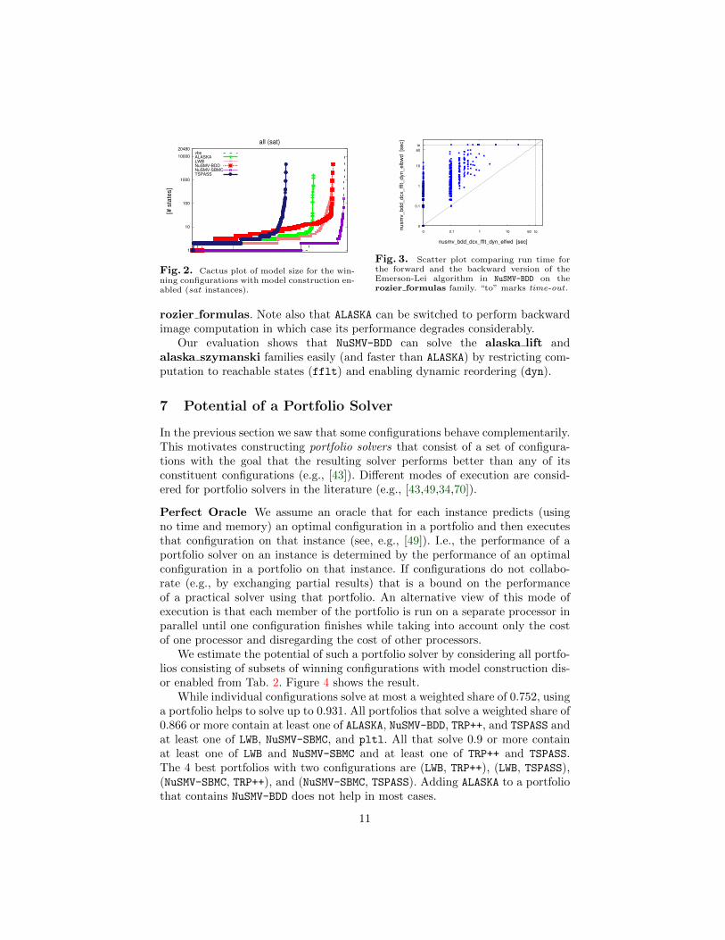
Track Model Construction Enabled We focus on model size. Figure 2 showsa cactus plot for the winning configurations with model construction enabled (satinstances). A vbs of all configurations with model construction enabled solves allbut the largest instances of anzu amba, anzu genbuf, and rozier counter.NuSMV-BDD is a sota based on instances in rozier counter; NuSMV-SBMC on in-stances in alaska lift, anzu amba, anzu genbuf, and rozier pattern; LWBon instances in rozier pattern.

95 % of the satisfiable instances have shortest models of size 3 or less. In-stances with shortest models of size larger than 11 are either from rozier coun-ter or from the variants in application modified to trigger meaningful behavior.

NuSMV-SBMC mostly produces shortest models, while NuSMV-BDD producesthe longest ones. On the other hand, NuSMV-BDD solves more instances of therozier counter family (which has very long models) than the other tools.

A Performance Advantage of ALASKA over NuSMV-BDD? In [69] De Wulfet al. perform a comparison between ALASKA and NuSMV-BDD for satisfiabil-ity and model checking of LTL. For LTL satisfiability they find that ALASKA

outperforms NuSMV-BDD on alaska lift, alaska szymanski, and a subfamily ofrozier formulas, while NuSMV-BDD performs better on rozier counter.

A comparison of the antichain-based algorithm in ALASKA [69] and theEmerson-Lei algorithm [30] used in NuSMV-BDD shows that the algorithm in[69] computes fixed points using forward image computation, while NuSMV-BDD

up to version 2.4.3 only uses (as is common) backward image computationsfor [30]. This triggered us to implement a forward version (e.g., [40]) of theEmerson-Lei algorithm in NuSMV-BDD. Figure 3 shows that the forward versionperforms considerably better than the backward version on the rozier formulasfamily. Using forward image computation NuSMV-BDD outperforms ALASKA on

10

1

10

100

1000

10000

20480

[#

sta

tes]

all (sat)

vbs

ALASKA

LWB

NuSMV-BDD

NuSMV-SBMC

TSPASS

Fig. 2. Cactus plot of model size for the win-ning configurations with model construction en-abled (sat instances).

0

0.1

1

10

60

to

0 0.1 1 10 60 to

nu

sm

v_b

dd

_d

cx_

fflt_d

yn

_elb

wd

[s

ec]

nusmv_bdd_dcx_fflt_dyn_elfwd [sec]

Fig. 3. Scatter plot comparing run time forthe forward and the backward version of theEmerson-Lei algorithm in NuSMV-BDD on therozier formulas family. “to” marks time-out.

rozier formulas. Note also that ALASKA can be switched to perform backwardimage computation in which case its performance degrades considerably.

Our evaluation shows that NuSMV-BDD can solve the alaska lift andalaska szymanski families easily (and faster than ALASKA) by restricting com-putation to reachable states (fflt) and enabling dynamic reordering (dyn).

7 Potential of a Portfolio Solver

In the previous section we saw that some configurations behave complementarily.This motivates constructing portfolio solvers that consist of a set of configura-tions with the goal that the resulting solver performs better than any of itsconstituent configurations (e.g., [43]). Different modes of execution are consid-ered for portfolio solvers in the literature (e.g., [43,49,34,70]).

Perfect Oracle We assume an oracle that for each instance predicts (usingno time and memory) an optimal configuration in a portfolio and then executesthat configuration on that instance (see, e.g., [49]). I.e., the performance of aportfolio solver on an instance is determined by the performance of an optimalconfiguration in a portfolio on that instance. If configurations do not collabo-rate (e.g., by exchanging partial results) that is a bound on the performanceof a practical solver using that portfolio. An alternative view of this mode ofexecution is that each member of the portfolio is run on a separate processor inparallel until one configuration finishes while taking into account only the costof one processor and disregarding the cost of other processors.

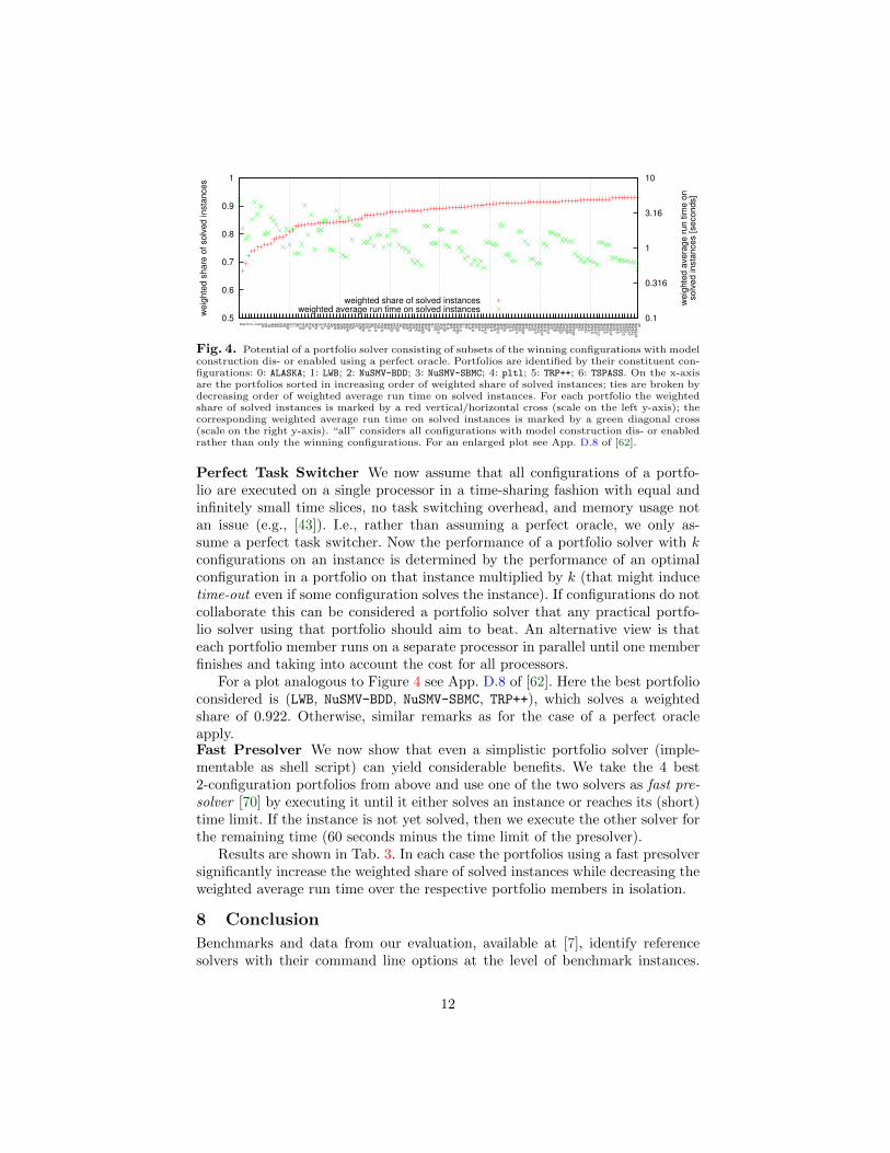
We estimate the potential of such a portfolio solver by considering all portfo-lios consisting of subsets of winning configurations with model construction dis-or enabled from Tab. 2. Figure 4 shows the result.

While individual configurations solve at most a weighted share of 0.752, usinga portfolio helps to solve up to 0.931. All portfolios that solve a weighted share of0.866 or more contain at least one of ALASKA, NuSMV-BDD, TRP++, and TSPASS andat least one of LWB, NuSMV-SBMC, and pltl. All that solve 0.9 or more containat least one of LWB and NuSMV-SBMC and at least one of TRP++ and TSPASS.The 4 best portfolios with two configurations are (LWB, TRP++), (LWB, TSPASS),(NuSMV-SBMC, TRP++), and (NuSMV-SBMC, TSPASS). Adding ALASKA to a portfoliothat contains NuSMV-BDD does not help in most cases.

11

0.5

0.6

0.7

0.8

0.9

1

0 6 4 3 1 2 50

20

40

15

60

60

50

33

405

61

31

44

601

303

42

601

42

504

61

201

22

402

44

504

502

602

545

604

56

25

613

42

302

302

56

12

301

23

36

01

34

12

401

24

34

603

603

46

23

402

34

35

35

603

503

56

34

534

56

03

45

034

56

24

602

46

16

12

34

012

34

24

502

45

01

614

624

56

024

56

01

46

15

15

601

501

56

14

514

56

01

45

014

56

12

601

26

12

46

012

46

23

602

36

12

501

25

12

56

012

56

23

46

023

46

13

613

46

12

45

012

45

124

56

012

45

601

36

013

46

23

502

35

23

56

023

56

23

45

023

45

234

56

023

45

613

513

56

13

45

134

56

01

35

013

45

013

56

013

45

612

36

012

36

123

46

012

34

612

35

012

35

123

45

012

34

51

23

56

012

35

61

23

45

60

12

34

56

all

0.1

0.316

1

3.16

10

weig

hte

d s

hare

of solv

ed insta

nces

weig

hte

d a

vera

ge r

un tim

e o

nsolv

ed insta

nces [seconds]

weighted share of solved instancesweighted average run time on solved instances

Fig. 4. Potential of a portfolio solver consisting of subsets of the winning configurations with modelconstruction dis- or enabled using a perfect oracle. Portfolios are identified by their constituent con-figurations: 0: ALASKA; 1: LWB; 2: NuSMV-BDD; 3: NuSMV-SBMC; 4: pltl; 5: TRP++; 6: TSPASS. On the x-axisare the portfolios sorted in increasing order of weighted share of solved instances; ties are broken bydecreasing order of weighted average run time on solved instances. For each portfolio the weightedshare of solved instances is marked by a red vertical/horizontal cross (scale on the left y-axis); thecorresponding weighted average run time on solved instances is marked by a green diagonal cross(scale on the right y-axis). “all” considers all configurations with model construction dis- or enabledrather than only the winning configurations. For an enlarged plot see App. D.8 of [62].

Perfect Task Switcher We now assume that all configurations of a portfo-lio are executed on a single processor in a time-sharing fashion with equal andinfinitely small time slices, no task switching overhead, and memory usage notan issue (e.g., [43]). I.e., rather than assuming a perfect oracle, we only as-sume a perfect task switcher. Now the performance of a portfolio solver with kconfigurations on an instance is determined by the performance of an optimalconfiguration in a portfolio on that instance multiplied by k (that might inducetime-out even if some configuration solves the instance). If configurations do notcollaborate this can be considered a portfolio solver that any practical portfo-lio solver using that portfolio should aim to beat. An alternative view is thateach portfolio member runs on a separate processor in parallel until one memberfinishes and taking into account the cost for all processors.

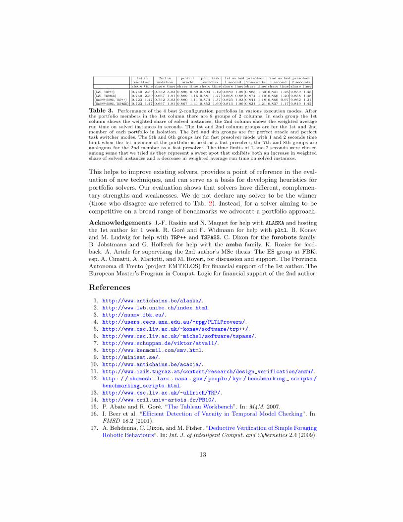
For a plot analogous to Figure 4 see App. D.8 of [62]. Here the best portfolioconsidered is (LWB, NuSMV-BDD, NuSMV-SBMC, TRP++), which solves a weightedshare of 0.922. Otherwise, similar remarks as for the case of a perfect oracleapply.Fast Presolver We now show that even a simplistic portfolio solver (imple-mentable as shell script) can yield considerable benefits. We take the 4 best2-configuration portfolios from above and use one of the two solvers as fast pre-solver [70] by executing it until it either solves an instance or reaches its (short)time limit. If the instance is not yet solved, then we execute the other solver forthe remaining time (60 seconds minus the time limit of the presolver).

Results are shown in Tab. 3. In each case the portfolios using a fast presolversignificantly increase the weighted share of solved instances while decreasing theweighted average run time over the respective portfolio members in isolation.

8 Conclusion

Benchmarks and data from our evaluation, available at [7], identify referencesolvers with their command line options at the level of benchmark instances.

12

1st in 2nd in perfect perf. task 1st as fast presolver 2nd as fast presolverisolation isolation oracle switcher 1 second 2 seconds 1 second 2 seconds

share time share time share time share time share time share time share time share time

(LWB, TRP++) 0.740 2.59 0.752 3.03 0.896 0.89 0.894 1.12 0.880 1.09 0.885 1.30 0.841 1.26 0.850 1.45(LWB, TSPASS) 0.740 2.59 0.667 1.91 0.889 1.16 0.881 1.27 0.868 0.88 0.874 1.10 0.850 1.20 0.858 1.48(NuSMV-SBMC, TRP++) 0.723 1.47 0.752 3.03 0.880 1.11 0.874 1.37 0.823 1.03 0.841 1.18 0.860 0.97 0.862 1.31(NuSMV-SBMC, TSPASS) 0.723 1.47 0.667 1.91 0.867 1.41 0.853 1.60 0.813 1.00 0.831 1.21 0.837 1.17 0.840 1.42

Table 3. Performance of the 4 best 2-configuration portfolios in various execution modes. Afterthe portfolio members in the 1st column there are 8 groups of 2 columns. In each group the 1stcolumn shows the weighted share of solved instances, the 2nd column shows the weighted averagerun time on solved instances in seconds. The 1st and 2nd column groups are for the 1st and 2ndmember of each portfolio in isolation. The 3rd and 4th groups are for perfect oracle and perfecttask switcher modes. The 5th and 6th groups are for fast presolver mode with 1 and 2 seconds timelimit when the 1st member of the portfolio is used as a fast presolver; the 7th and 8th groups areanalogous for the 2nd member as a fast presolver. The time limits of 1 and 2 seconds were chosenamong some that we tried as they represent a sweet spot that exhibits both an increase in weightedshare of solved instances and a decrease in weighted average run time on solved instances.

This helps to improve existing solvers, provides a point of reference in the eval-uation of new techniques, and can serve as a basis for developing heuristics forportfolio solvers. Our evaluation shows that solvers have different, complemen-tary strengths and weaknesses. We do not declare any solver to be the winner(those who disagree are referred to Tab. 2). Instead, for a solver aiming to becompetitive on a broad range of benchmarks we advocate a portfolio approach.

Acknowledgements J.-F. Raskin and N. Maquet for help with ALASKA and hostingthe 1st author for 1 week. R. Gore and F. Widmann for help with pltl. B. Konevand M. Ludwig for help with TRP++ and TSPASS. C. Dixon for the forobots family.B. Jobstmann and G. Hofferek for help with the amba family. K. Rozier for feed-back. A. Artale for supervising the 2nd author’s MSc thesis. The ES group at FBK,esp. A. Cimatti, A. Mariotti, and M. Roveri, for discussion and support. The ProvinciaAutonoma di Trento (project EMTELOS) for financial support of the 1st author. TheEuropean Master’s Program in Comput. Logic for financial support of the 2nd author.

References

1. http://www.antichains.be/alaska/.2. http://www.lwb.unibe.ch/index.html.3. http://nusmv.fbk.eu/.4. http://users.cecs.anu.edu.au/~rpg/PLTLProvers/.5. http://www.csc.liv.ac.uk/~konev/software/trp++/.6. http://www.csc.liv.ac.uk/~michel/software/tspass/.7. http://www.schuppan.de/viktor/atva11/.8. http://www.kenmcmil.com/smv.html.9. http://minisat.se/.

10. http://www.antichains.be/acacia/.11. http://www.iaik.tugraz.at/content/research/design_verification/anzu/.12. http : / / shemesh . larc . nasa . gov / people / kyr / benchmarking _ scripts /

benchmarking_scripts.html.13. http://www.csc.liv.ac.uk/~ullrich/TRP/.14. http://www.cril.univ-artois.fr/PB10/.15. P. Abate and R. Gore. “The Tableau Workbench”. In: M4M. 2007.16. I. Beer et al. “Efficient Detection of Vacuity in Temporal Model Checking”. In:

FMSD 18.2 (2001).17. A. Behdenna, C. Dixon, and M. Fisher. “Deductive Verification of Simple Foraging

Robotic Behaviours”. In: Int. J. of Intelligent Comput. and Cybernetics 2.4 (2009).

13

18. D. Le Berre and L. Simon. “The Essentials of the SAT 2003 Competition”. In:SAT. Vol. 2919. LNCS. Springer, 2003.

19. D. Le Berre et al. “The SAT 2009 competition results: does theory meet practice?(presentation)”. In: SAT. Vol. 5584. LNCS. Springer, 2009.

20. A. Biere and K. Claessen. “Hardware Model Checking Competition (presenta-tion)”. In: Hardware Verification Workshop 2010, Edinburgh, UK, 2010. 2010.

21. A. Biere and T. Jussila. Benchmark Tool Run. http://fmv.jku.at/run/.22. A. Biere et al. Handbook of Satisfiability. IOS Press, 2009.23. R. Bloem et al. “Automatic hardware synthesis from specifications: a case study”.

In: DATE. 2007.24. R. Bloem et al. “Specify, Compile, Run: Hardware from PSL”. In: COCV.

Vol. 190(4). ENTCS. Elsevier, 2007.25. A. Cimatti et al. “Boolean Abstraction for Temporal Logic Satisfiability”. In:

CAV. Vol. 4590. LNCS. Springer, 2007.26. A. Cimatti et al. “NuSMV 2: An OpenSource Tool for Symbolic Model Checking”.

In: CAV. Vol. 2404. LNCS. Springer, 2002.27. E. Clarke, O. Grumberg, and K. Hamaguchi. “Another Look at LTL Model Check-

ing”. In: FMSD 10.1 (1997).28. M. Daniele, F. Giunchiglia, and M. Vardi. “Improved Automata Generation for

Linear Temporal Logic”. In: CAV. Vol. 1633. LNCS. Springer, 1999.29. E. Emerson. “Temporal and Modal Logic”. In: Handbook of Theoretical Computer

Science, Volume B: Formal Models and Sematics (B). 1990.30. E. Emerson and C. Lei. “Efficient Model Checking in Fragments of the Proposi-

tional Mu-Calculus (Extended Abstract)”. In: LICS. 1986.31. E. Filiot, N. Jin, and J. Raskin. “An Antichain Algorithm for LTL Realizability”.

In: CAV. Vol. 5643. LNCS. Springer, 2009.32. M. Fisher, C. Dixon, and M. Peim. “Clausal temporal resolution”. In: ACM Trans.

Comput. Log. 2.1 (2001).33. D. Fisman et al. “A Framework for Inherent Vacuity”. In: HVC. Vol. 5394. LNCS.

Springer, 2008.34. C. Gomes and B. Selman. “Algorithm portfolios”. In: Artif. Intell. 126.1-2 (2001).35. V. Goranko, A. Kyrilov, and D. Shkatov. “Tableau Tool for Testing Satisfiability

in LTL: Implementation and Experimental Analysis”. In: M4M. 2009.36. R. Gore. Personal Communication. 2010.37. R. Gore and F. Widmann. “An Experimental Comparison of Theorem Provers

for CTL”. In: CLoDeM. 2010.38. R. Gore and F. Widmann. “An Optimal On-the-Fly Tableau-Based Decision Pro-

cedure for PDL-Satisfiability”. In: CADE. Vol. 5663. LNCS. Springer, 2009.39. K. Heljanko, T. Junttila, and T. Latvala. “Incremental and Complete Bounded

Model Checking for Full PLTL”. In: CAV. Vol. 3576. LNCS. Springer, 2005.40. T. Henzinger, O. Kupferman, and S. Qadeer. “From Pre-Historic to Post-Modern

Symbolic Model Checking”. In: FMSD 23.3 (2003).41. A. Heuerding et al. “Propositional Logics on the Computer”. In: TABLEAUX.

Vol. 918. LNCS. Springer, 1995.42. B. Hirsch and U. Hustadt. “Translating PLTL into WS1S: Application Descrip-

tion”. In: M4M. 2001.43. B. Huberman, R. Lukose, and T. Hogg. “An Economics Approach to Hard Com-

putational Problems”. In: Science 275.5296 (1997).44. U. Hustadt and B. Konev. “TRP++: A temporal resolution prover”. In: Collegium

Logicum. Vol. 8. Kurt Godel Society, 2004.

14

45. U. Hustadt and R. A. Schmidt. “Formulae which Highlight Differences betweenTemporal Logic and Dynamic Logic Provers”. In: Issues in the Design and Ex-perimental Evaluation of Systems for Modal and Temporal Logics. Dipartimentodi Ingegneria dell’Informazione, Unversita degli Studi di Siena, 2001.

46. U. Hustadt and R. A. Schmidt. “Scientific Benchmarking with Temporal LogicDecision Procedures”. In: KR. Morgan Kaufmann, 2002.

47. U. Hustadt et al. “TeMP: A Temporal Monodic Prover”. In: IJCAR. Vol. 3097.LNCS. Springer, 2004.

48. G. Janssen. “Logics for Digital Circuit Verification: Theory, Algorithms, and Ap-plications”. PhD thesis. Technische Universiteit Eindhoven, 1999.

49. K. Leyton-Brown et al. “A Portfolio Approach to Algorithm Selection”. In: IJCAI.Morgan Kaufmann, 2003.

50. M. Ludwig and U. Hustadt. “Fair Derivations in Monodic Temporal Reasoning”.In: CADE. Vol. 5663. LNCS. Springer, 2009.

51. M. Ludwig and U. Hustadt. “Implementing a fair monodic temporal logic prover”.In: AI Commun. 23.2-3 (2010).

52. M. Ludwig and U. Hustadt. “Resolution-Based Model Construction for PLTL”.In: TIME. 2009.

53. L. de Moura. SAL: Tutorial. 2004.54. L. de Moura et al. “SAL 2”. In: CAV. Vol. 3114. LNCS. Springer, 2004.55. M. Nikolic. “Statistical Methodology for Comparison of SAT Solvers”. In: SAT.

Vol. 6175. LNCS. Springer, 2010.56. I. Pill et al. “Formal analysis of hardware requirements”. In: DAC. 2006.57. Prosyd. http://www.prosyd.org/.58. L. Pulina and A. Tacchella. “A self-adaptive multi-engine solver for quantified

Boolean formulas”. In: Constraints 14.1 (2009).59. K. Rozier and M. Vardi. “A Multi-encoding Approach for LTL Symbolic Satisfi-

ability Checking”. In: FM. Vol. 6664. LNCS. Springer, 2011.60. K. Rozier and M. Vardi. “LTL Satisfiability Checking”. In: STTT 12.2 (2010).61. V. Schuppan. “Towards a notion of unsatisfiable and unrealizable cores for LTL”.

In: Sci. Comput. Program. In Press (2010). doi: 10.1016/j.scico.2010.11.004.62. V. Schuppan and L. Darmawan. Evaluating LTL Satisfiability Solvers (full ver-

sion). http://www.schuppan.de/viktor/VSchuppanLDarmawan- ATVA- 2011-

full.pdf. 2011.63. S. Schwendimann. “A New One-Pass Tableau Calculus for PLTL”. In:

TABLEAUX. Vol. 1397. LNCS. Springer, 1998.64. L. Simon and D. Le Berre. “Some Results and Lessons from the SAT Competi-

tions (invited talk, slides only)”. In: Second International Workshop on ConstraintPropagation and Implementation, Sitges, Spain, October 1, 2005. 2005.

65. StatSoft, Inc. Electronic Statistics Textbook. StatSoft, Tulsa, OK, USA. Availablefrom http://www.statsoft.com/textbook/.

66. G. Sutcliffe and C. Suttner. “Evaluating general purpose automated theorem prov-ing systems”. In: Artif. Intell. 131.1-2 (2001).

67. The VIS Group. “VIS: A System for Verification and Synthesis”. In: CAV.Vol. 1102. LNCS. Springer, 1996.

68. P. Wolper. “The Tableau Method for Temporal Logic: An Overview”. In: Logiqueet Analyse 28.110–111 (1985).

69. M. De Wulf et al. “Antichains: Alternative Algorithms for LTL Satisfiability andModel-Checking”. In: TACAS. Vol. 4963. LNCS. Springer, 2008.

70. L. Xu et al. “SATzilla: Portfolio-based Algorithm Selection for SAT”. In: JAIR32 (2008).

15