evaluating model fit in bayesian confirmatory factor ... · pdf filewith cfa the underlying...
TRANSCRIPT
EVALUATING BAYESIAN CFA USING THE BRMSEA 1
Evaluating model fit in Bayesian confirmatory factor analysis with large
samples: Simulation study introducing the BRMSEA
Huub Hoofs
Department of Epidemiology, CAPHRI School for Public Health and Primary Care, Faculty of
Health, Medicine and Life Sciences, Maastricht University, Maastricht, The Netherlands &
Academic Collaborative Centre for Public Health Limburg, Public Health Service Southern
Limburg, Geleen, The Netherlands
Rens van de Schoot
Department of Methods and Statistics, Faculty of Social Sciences, Utrecht University, Utrecht,
Netherlands & Optentia Research Program, Faculty of Humanities, North-West University,
Vanderbijlpark, South Africa
Nicole W. H. Jansen and IJmert Kant
Department of Epidemiology, CAPHRI School for Public Health and Primary Care, Faculty of
Health, Medicine and Life Sciences, Maastricht University, Maastricht, The Netherlands
Correspondence to H. Hoofs, Department of Epidemiology, School CAPHRI, Maastricht
University, P.O. Box 616, 6200 MD Maastricht, The Netherlands, Telephone: +31(0)433882368
Email: [email protected]
The authors would like to thank Dave Stynen and Andrea Brouwers for reading and criticizing the
preliminary draft of the manuscript. H.H. was supported by a grant from the province Limburg
(CWZW2011/57962), the School for Public Health and Primary Care (CAPHRI; Maastricht), and GGD
Zuid-Limburg. R.v.d.S. was supported by a grant from the Netherlands organization for scientific research
(NWO-VENI-451-11-008). Author contributions: H.H. and R.v.d.S. developed the concept; H.H. and
R.v.d.S. designed simulation study; H.H. performed analysis for the simulation study and empirical
illustration; R.v.d.S. supervised the analysis; H.H. wrote the paper; N.W.H.J. and IJ.K. conducted the data
collection of the empirical illustration; R.v.d.S., N.W.H.J., and IJ.K. edited and supervised the construction
of the manuscript. All authors contributed extensively to the work presented in this paper.

EVALUATING BAYESIAN CFA USING THE BRMSEA 2
Evaluating model fit in Bayesian confirmatory factor analysis with large
samples: Simulation study introducing the BRMSEA
Bayesian confirmatory factor analysis (CFA) offers an alternative to frequentist CFA based
on, for example, Maximum Likelihood estimation for the assessment of reliability and
validity of educational and psychological measures. For increasing sample sizes, however,
the applicability of current fit statistics evaluating model fit within Bayesian CFA is limited.
We propose, therefore, a Bayesian variant of the root mean square error of approximation
(RMSEA), the BRMSEA. A simulation study was performed with variations in model
misspecification, factor loading magnitude, number of indicators, number of factors, and
sample size. This showed that the 90% posterior probability interval of the BRMSEA is valid
for evaluating model fit in large samples (N ≥ 1,000), using cut-off values for the lower (<
.05) and upper limit (< .08) as guideline. An empirical illustration further shows the
advantage of the BRMSEA in large sample Bayesian CFA models. In conclusion it can be
stated that the BRMSEA is well suited to evaluate model fit in large sample Bayesian CFA
models by taking sample size and model complexity into account.
Keywords: Bayesian procedures, Factor analysis, Model fit, Validity, Simulation
Introduction
Educational and psychological measures often include multiple indicators consisting of items from
a questionnaire, a set of observations, or results from an interactive application. These indicators
are believed to represent (multiple) latent factor(s) which are not directly observable. The
Classroom Assessment Scoring System Toddler (CLASS; Pianta, Hamre, & La Paro, 2011), for
example, combines observations on different domains to provide an indication of the educational
and emotional quality in the classroom. Confirmatory factor analysis (CFA) plays an important
role in the assessment of the reliability and validity of such measures (DiStefano & Hess, 2005).
With CFA the underlying theoretical framework of an instrument can be assessed providing a
transparent and theoretical description of its (psychometric) properties (e.g., Kline, 2011). As such
EVALUATING BAYESIAN CFA USING THE BRMSEA 3
CFA gives insight in, for example, the relation between indicators and the latent factor(s), the
(hierarchical) factor structure, and potential interdependencies between indicators of educational
and psychological measures. Besides these aspects, CFA can also assess the validity of an
instrument across groups and over time. This aspect, known as measurement
equivalence/invariance (ME/I), indicates if an instrument measures the same (latent) construct
across different populations or settings (Millsap, 2011; Van de Schoot, De Beuckelaer, Lek, &
Zondervan-Zwijnenburg, 2015). As such CFA plays an important role within the development,
validation, and application of most measurement instruments.
While CFA is classically performed within a frequentist framework, recent decades have
seen a strong increase in the use of the Bayesian framework to estimate CFA (Van de Schoot,
Winter, Ryan, Zondervan-Zwijnenburg, & Depaoli, 2016). Within large samples with normally
distributed data which is not impacted by a high proportion of outliers or missingness Bayesian
CFA and frequentist CFA have roughly the same results (Scheines, Hoijtink, & Boomsma, 1999).
Bayesian CFA can however offer several advantages over the frequentist approach such as
computational advantages and intuitive interpretation of the results (Muthén & Asparouhov, 2012;
Van de Schoot et al., 2014). Bayesian CFA also enables new modelling approaches (Muthén &
Asparouhov, 2012), such as approximate invariance (i.e. alignment; Muthén & Muthén, 2013; Van
de Schoot et al., 2013). Researchers can, furthermore, incorporate background knowledge into
their analyses, through the specification of prior information (e.g., Van de Schoot et al., 2014). As
such, Bayesian CFA can ‘simply’ be used as a different estimator, but it can also provide access to
CFA models that are not feasible within a frequentist framework (Kaplan & Depaoli, 2012). While
the application of Bayesian CFA is on the rise, some issues warrant further research. One of these
aspects is the objective assessment of overall model fit within large samples. While current
measures for model fit within Bayesian CFA show positive properties within studies with small

EVALUATING BAYESIAN CFA USING THE BRMSEA 4
samples, within large samples, surpassing 1,000 subjects, the sensitivity of the overall fit statistic
to detect negligible differences between the observed data and the hypothesized model is high
(Hoijtink & Van de Schoot, in press). Within empirical settings, in which negligible deviations
from the hypothesized model are always expected, an increase in sample size inevitably leads
therefore to a deterioration of model fit (MacCallum, 2003). That is, acceptance rates of models
with a “small” misspecification (e.g. non-specified negligible cross-loading) decrease with
increasing sample size (Asparouhov & Muthen, 2010). For applied research this makes it difficult
to objectively assess, interpret, and communicate the quality of the model. Consider, for example,
that the CLASS would be compared across different countries with a large number of
measurements per country in the study. As within empirical studies discrepancy between the
hypothesized and observed model is expected, this would result in a deteriorated model fit. This
could result in false conclusion with regard to the validity and application of the instrument across
countries. While overall model fit is not synonymous with model quality, it constitutes an
important and integral part of it (Bentler, 2007; Millsap, 2007). The current study introduces and
validates a fit measure, the Bayesian Root Mean Square Error of Approximation (BRMSEA),
which is less sensitive for large samples. This could improve assessment of overall model fit
within Bayesian CFA with large samples, enhancing application of this framework to provide
insight regarding the reliability and validity of measurement instruments.
Evaluation of the model fit within Bayesian CFA relies on the validity of the model for
future observations (Kaplan & Depaoli, 2012). To simulate such future observations, replications
of the observed data are generated (Levy, 2011). The χ2 for the observed and replicated (or
updated) data is subsequently computed for each iteration within the Markov Chain (Levy, 2011).
Within Bayesian CFA the posterior predictive p-value (ppp) checks the proportion of iterations for
which the replicated χ2 exceeds the observed χ2 (for other implementations of the ppp see, Gelman,

EVALUATING BAYESIAN CFA USING THE BRMSEA 5
Carlin, Stern, & Rubin, 2014; Lee, 2007). A “good” fit is indicated if the ppp is around .50
(Gelman et al., 2014; Muthén & Asparouhov, 2012). The ppp is found to be robust for assessing
model fit within small samples (Asparouhov & Muthén, 2010; Lee & Song, 2004; Rupp, Dey, &
Zumbo, 2004). It is especially through these characteristics, including the use of priors, that
Bayesian CFA works so well in small samples as it is not based on large-sample theory. For large
samples it seems however that the ppp becomes sensitive for trivial deviations from the
hypothesized model (Hoijtink & Van de Schoot, in press). A simulation study by Asparouhov and
Muthén (2010) showed, for example, that despite the robustness of the ppp for models with a
“minor” misspecification for larger samples compared to p-values within frequentist CFA,
rejection rates still increase. In this study a “minor” misspecification was defined as the omission
of standardized cross-loadings smaller than .1 within a CFA. Rejection rates increased with
increasing sample sizes (N = 300, 500, and 1,000) both for frequentist CFA (19%, 21%, and 44%
respectively) and Bayesian CFA (6%, 12%, and 29% respectively). While studies within Bayesian
CFA regarding this phenomenon, or the functioning of model fit in general, are underrepresented
(Levy, 2011; Rindskopf, 2012), it seems that the sensitivity of the ppp to detect negligible
differences within large samples approaches 1.0. As such, it seems the ppp is well suitable for
studies with small to moderate samples, but loses it salience within studies using large samples.
To resolve this problem within frequentist CFA, fit indices are frequently used (Bentler,
1990; Kline, 2011). Fit indices provide, on a continuous scale, a quantitative measure of model fit.
In general terms it can be stated that they provide a credibility check of models while taking into
account the overall and specific discrepancy between the model and the population (MacCallum,
2003). The first criterion for such fit indices is that they should not be penalized for an increasing
sample size (Marsh, Balla, & McDonald, 1988). The second criterion is the correction for model
complexity to ensure that there is no free lunch regarding the inclusion of extra parameters –

EVALUATING BAYESIAN CFA USING THE BRMSEA 6
which always improves model fit (Browne & Cudeck, 1992). Fit indices provide a goodness or a
badness-of-fit. In the former, a higher value (often towards 1) indicates a better fitting model while
in the latter, a lower value (often towards 0) indicates a better fitting model (West, Taylor, & Wu,
2012). Facilitating the interpretation of fit indices cut-off values are proposed indicating “good”,
“acceptable”, and “poor” fit (Browne & Cudeck, 1992; Hu & Bentler, 1999).
It should be noted that there is a long-standing and ongoing discussion about fit indices
(e.g., Barrett, 2007). This debate particularly focuses on the reliance on indicative thresholds (or
cut-off points) as golden rules, but also on the neglect of the predictive quality of the models and
the negligence with respect to a significant χ2 (e.g., Fan & Sivo, 2007; Marsh, Hau, & Wen, 2004;
McDonald & Ho, 2002). In line with Lai and Green (2016), quotation marks are therefore used in
the present article for quantifications of model fit (e.g. “good” model) and misspecification (e.g.
“large” misspecification) to indicate the ambiguity of such qualifications. Notwithstanding
theoretical and statistical criticisms, fit indices can play however a crucial, but not solitary, role in
in the assessment of model quality as qualitative judgment about the overall model fit (e.g.,
Bentler, 2007; Kline, 2011; Millsap, 2007; Yuan, 2005). Without such quantifications, the
judgment of model quality within large sample Bayesian CFA models relies almost solely on
subjective measures. Thresholds provide a standard – which is ambiguous by nature – enabling
transparent assessment and communication of model quality. A fit index which is robust to an
increased sample size is therefore crucial as it would lead to an improved understanding of model
fit and accessibility for Bayesian CFA within large samples (e.g., Cieciuch, Davidov, Schmidt,
Algesheimer, & Schwartz, 2014; Milojev, Osborne, Greaves, Barlow, & Sibley, 2013; Lung,
Chiang, Lin, Shu, & Lee, 2011). Assessing model quality in such samples would be greatly
enhanced by a fit index which is informative within large samples.
EVALUATING BAYESIAN CFA USING THE BRMSEA 7
The present article is the first to explore whether the rationale of such a fit index (i.e. the
RMSEA) can be applied within Bayesian CFA (i.e. the BRMSEA) to provide a valid evaluation of
model fit within large samples. The motivation to implement the rationale of the RMSEA within
Bayesian CFA is threefold. First, within frequentist CFA the RMSEA has been shown to work
especially well with large samples (Chen, Curran, Bollen, Kirby, & Paxton, 2008; Curran, Bollen,
Chen, Paxton, & Kirby, 2003; MacCallum, Browne, & Sugawara, 1996), which is exactly the area
in which the ppp become less useful. Second, the RMSEA is an absolute fit index and does
therefore not require a baseline, or empty, model (Steiger & Lind, 1980; West et al., 2012). Such a
baseline model would be contradictory with the Bayesian framework regarding the inclusion of
prior knowledge of the model. Third, the RMSEA enables the computation of a confidence
interval (CI) which provides information regarding the trustworthiness of the model fit (Browne &
Cudeck, 1992; Steiger, 1990, 2000). This enhances comparability as this corresponds to the
approach within the Bayesian framework of reporting posterior probability intervals (PPI; Van de
Schoot et al., 2014). While not mathematically equivalent, the PPI and the CI serve related
inferential goals. These aspects support the implementation of the BRMSEA as a fit index within
Bayesian CFA. Additionally, the BRMSEA should also function in accordance with the prior
specification of a model, as this influences the overall fit and complexity of a model
(Spiegelhalter, Best, Carlin, & Van Der Linde, 2002). Correct and informative priors should
therefore positively affect the BRMSEA and vice-versa. It is hypothesized that the BRMSEA
accurately assesses model fit in Bayesian CFA within large samples while the ppp in contrast loses
its salience for such samples.
EVALUATING BAYESIAN CFA USING THE BRMSEA 8
Technical Background of the RMSEA and the BRMSEA
Background of the RMSEA
Throughout the Technical Background a parameter with a hat (^) indicates the estimation of a
population parameter. The RMSEA stems from the work by Steiger and Lind (1980) who explored
the fit of a model, derived from a sample, in relation to the fit of the model in the true population.
The fit (statistic) of a model within the population is defined as F0. If a model does not show
perfect fit, which is to be expected in empirical settings, an estimate of F0 has to be derived (𝐹").
Browne & Cudeck (1992) argue that the sample fit (𝐹) of a model can be used to estimate the fit
statistic (𝐹"):
𝐹" = (𝐹 − 𝑑)/(𝑁 − 1), (1)
in which d is the number of free parameters and N the sample size. Equation 1 is under the
assumption that 𝐹" indicates the degree of lack of fit taking into account the lack of fit arising due
to sampling error. As such this estimation of 𝐹" takes the number of free parameters and the
sample size into account to estimate the misfit of a model in the population. Browne and Cudeck
(1992) further state that the model fit of a population decreases if free parameters (q) are added.
These two premises result in a measure of discrepancy of the model per free parameter (ε)
(Browne & Cudeck, 1992), defined as
𝜀 = ,-d
(2)
which prefers parsimonious models. That is, if two models have the same fit within the population
the model with fewer estimated parameters will yield a smaller value (MacCallum et al., 1996). To
estimate F0 in Equation 2 it can be substituted as
EVALUATING BAYESIAN CFA USING THE BRMSEA 9
𝜀 = ,/0d(N-1)
. (3)
As it is possible that the numerator is negative, an added condition is that if 𝑑 > 𝐹 the 𝜀 is set to
zero. This results in a theoretical range of 𝜀 from zero to infinity in which a value of zero denotes a
perfect fitting model, while larger values reflect a poor model fit (badness-of-fit).
Implementation of the RMSEA within frequentist CFA
Within the frequentist framework the 𝜀 from Equation 3 is referred to as the RMSEA which uses
the χ2 to reflect the degree of misfit (𝐹; Equation 3):
RMSEA = 9:/dfdf(N-1)
. (4)
In Equation 4 df (degrees of freedom) reflects the number of free parameters in the model:
df = 𝑝 − 𝑞. (5)
With p being the number of number of observations, defined as the number of unique elements
within the sample variance-covariance matrix (v[v+1]/2) and q the number of free (estimated)
parameters. If the mean structure is included, this number is summed with the number of (v)
observed variables (Kline, 2011).
The 𝐹 from Equation 3 can also be replaced with the misfit from the general least square
(GLS) or asymptotically distribution free (ADF) instead of the maximum likelihood (ML) based χ2
(Browne & Cudeck, 1992). Commonly used cut-off points for the RMSEA are values below 0.05
denoting good model fit, values below 0.08 denoting adequate model fit. Hu and Bentler (1999)
suggested that for a good model fit a cut-off point of 0.06 could also be used.
EVALUATING BAYESIAN CFA USING THE BRMSEA 10
A key strength of the RMSEA is that the sampling distribution is known under certain
assumptions. Support for this notion is based on the fact that the asymptotic distribution of
RMSEA is a re-scaled χ2 for a given sample size, df, and a noncentrality parameter λ (Browne &
Cudeck, 1992). The lower (LL) and upper limit (UL) of the RMSEA CI are given as
RMSEACI =@LL
df(N-1); @UL
df(N-1). (6)
This CI enables the test whether a model exhibits close or worse fit, which is achieved when the
lower limit is below or above a certain threshold (Browne & Cudeck, 1992).
Implementation of the BRMSEA within Bayesian CFA
Inspired by Browne and Cudeck (1992) who stated that different measures of discrepancy (i.e. χ2)
can be used for the estimation of ε̂ from Equation 3, we propose that it can also be applied within
Bayesian CFA. Hence, the fact that the RMSEA was developed and applied within a frequentist
framework does not hinder the implementation of its rationale within the Bayesian framework.
The notion that the degree of misfit (𝐹) should be rescaled according to the number of estimated
parameters (d) and sample size (N) is therefore implemented within Bayesian CFA. Within a
Bayesian framework there is, however, no classical discrepancy function or df. This section
illustrates the parameters from a Bayesian CFA framework which are implemented in Equation 3
to achieve a Bayesian variant of the RMSEA the BRMSEA.
With regards to model misfit (𝐹), for which the χ2 is used within the frequentist framework
(Equation 5), the difference between the observed and replicated χ2 (𝜒obsHI − 𝜒repH
I ) for each
iteration (i; after burn-in) is used for the BRMSEA. Within Bayesian CFA this difference can be
regarded as the degree of misfit (𝐹) in Equation 3. Similar to a classical discrepancy function, such
EVALUATING BAYESIAN CFA USING THE BRMSEA 11
as the χ2 within frequentist CFA, 𝜒obsHI − 𝜒repH
I will positively increase with increasing levels of
misfit. In contrast to classical discrepancy function, such as the χ2 within frequentist CFA, 𝜒obsHI −
𝜒repHI can be negative for an iteration. For multiple iterations, however, 𝜒obsI − 𝜒repI will
approximately result in 0 for a perfect fitting model and will positively increase with increasing
levels of misfit, similar to a classical discrepancy function.
To control for model complexity, it is important to include the effect that prior information
has on the estimation process, as prior information can alter the “effective” number of estimated
parameters. A prior with a mean of zero and a very small variance is, for example, nearly equal to
a parameter which is fixed to zero (Asparouhov, Muthen, & Morin, 2015). Especially if a
multitude of such priors are used, the difference between the number of estimated parameters and
the effective number of estimated parameters can become substantial. To correct for this effect
within Bayesian CFA the effective number of parameters (pD; Spiegelhalter et al., 2002) are used.
The pD parameter is developed in conjunction with the deviance information criterion (DIC) as
penalty term for complexity. Subtracting the pD, instead of q (Equation 5), from the number of
observations (p) gives a fair estimation of the effective model complexity within Bayesian CFA.
Equivalent models with differing prior information will, therefore, have a different model
complexity which is in line with the Bayesian framework.
Combining the model fit of Bayesian CFA (𝜒obsHI − 𝜒repH
I ) with the effective number of
parameters (pD) results in the following equation for the BRMSEA:
BRMSEAN =9obsH: /9repH
: /(P/PQ)
(P/PQ)(R/S). (7)
EVALUATING BAYESIAN CFA USING THE BRMSEA 12
As such, the BRMSEA results in a set of (i) rescaled differences between the observed and
replicated χ2, taking into account the (effective) number of estimated parameters and sample size.
By doing so it provides an estimation of the validity of the model for the population while taking
into account the lack of fit arising due to sampling error. The numerator of the BRMSEA will be
set at 0 for an iteration if it is negative. As 𝜒obsI − 𝜒repI will on average be 0 in a perfect fitting
model, the BRMSEA will also be zero for perfectly fitting models, and positively increase towards
infinity for increasing levels of misspecification.
In contrast to the frequentist framework, in which the CI of the RMSEA is commonly
computed on the basis of asymptotic theory, the PPI of the BRMSEA should be derived, as any
posterior measure within Bayesian CFA, from the posterior density. The PPI (e.g. 90%) of the
BRMSEA is extracted from the total set of iterations. In the present study the lower limit is 5%
and the upper limit 95%, as the used PPI of the BRMSEA is 90%. This 90% is in line with the
90% CI often used for the RMSEA (Browne & Cudeck, 1992). Due to the (theoretical)
comparability of the RMSEA and BRMSEA it is hypothesized that their functioning regarding the
assessment of overall model fit is equivalent. A simulation study is proposed to empirically test
this hypothesized functioning of the BRMSEA within Bayesian CFA.
Simulation Study
In this article the validity of the BRMSEA within a Bayesian CFA is evaluated (see Supplement A
for R-code). The characteristics of the BRMSEA and the ppp are examined within various
conditions in a simulation study. It is hypothesized that for large samples the ppp rejects all
models with any form of (“small”) misspecification while the BRMSEA only rejects models
which a “large” misspecification and accepts models with a “small” misspecification. The
comparison with the RMSEA is made to see whether its characteristics are analogous with those of
EVALUATING BAYESIAN CFA USING THE BRMSEA 13
the BRMSEA. The frequentist χ2 based p-value and the Bayesian ppp are expected to reject all
models with any form of misspecification. Implementation of the BRMSEA will be further
facilitated and evaluated by the implementation of cut-off points.
Methods
Data generation
The simulation study consisted of two sections. In the first section different population covariance
matrices (conditions) were tested against a common 1-factor CFA model. In the second section a
partly different set of conditions was tested against a 2-factor CFA model.
The different population covariance matrices (conditions) in the first section, which were
tested against a common 1-factor CFA model (Figure 1A), were specified varying the following
four aspects: (1) Specification of the population factor model (Model A, B, C, D, and E; see Figure
1), (2) number of indicators (6 and 12), (3) magnitude of factor loadings (.5 and .7), and (4)
sample size (50, 100, 250, 500, 1,000, 5,000, and 10,000). The specification of the population
factor models (partly based on, Shevlin & Miles, 1998), which were used to generate the data,
were increasingly different compared to a common 1-factor model. Specification B and C were
regarded as “small” misspecifications as the residual correlation was .1 and the salient pattern of
the factor loadings corresponded with that of the reference model (Heene, Hilbert, Freudenthaler,
& Bühner, 2012). The number of residual correlation, especially for specification B, was
furthermore limited. Specification D and especially E were seen as models with more substantial
(“large”) amounts of misspecification, primarily because the difference in the salient pattern of the
factor structure and the moderate correlation between these factors.
For the second section the reference models was a 2-factor model (specification D; Figure
1D). In this section the number of indicators (i.e., 12) and the magnitude of factor loadings (i.e.,

EVALUATING BAYESIAN CFA USING THE BRMSEA 14
.7) were not varied and were based on the findings in the first section. Sample size variation was
equal to that in the first section. Specification of the population factor model, partly based on
Asparouhov and Muthen (2010), consisted of four models (Model D, E, F1, and F2). Models F1
and F2 were similar to model D except the inclusion of cross loadings between the sixth indicator
and the second factor and the seventh indicator and the first factor (Figure 1). These cross loadings
were “small” and 10% of the salient factor loadings in model F1 (.07) and “moderate” in model F2
(.35). The “small” cross loadings in model F1 should result in a rejection of the model whilst the
standardized cross loadings above .3 in model F2 should result in a majority the models being
rejected (Asparouhov & Muthen, 2010; Saris, Satorra, Van der Veld, 2009). Specifications A
through C were not tested against the reference model in the second section as this would be
complicated by the freely estimated covariance between the two factors, which would approach 1
in these models, resulting in a bias in parameter estimates but not in overall model fit.
All models were identified through constraining the factor variance(s) to 1. Intercepts of all
indicators and latent factor means were specified to be zero. Residuals were estimated through
subtracting 1 with the associated magnitude of the factor loadings squared. The different variations
(i.e. specification, number of indicators, magnitude of factor loadings, and sample size) resulted in
a total of 140 (5 × 2 × 2 × 7) different conditions in the first section and 28 (4 × 1 × 1 × 7) in the
second section. For each condition 500 samples were generated. Cumulative averages plots
indicated that the number of samples was sufficient as estimates were fully stabilized by 500
samples. Population RMSEA for the various conditions, in both sections, are presented in Table 1.
Estimation and prior specification
In both sections two estimators were used, that is maximum likelihood (ML) for the frequentist
CFA and Bayesian estimation for the Bayesian CFA. For the Bayesian estimation, three variations

EVALUATING BAYESIAN CFA USING THE BRMSEA 15
regarding the specification of priors were examined. Differentiation in prior specification was
simulated to examine the effect of priors on the characteristics of the BRMSEA. The first variation
included the default, diffuse priors of Mplus which are N(0,∞) for the intercepts and factor
loadings, and IG(-1, 0) for residual variances (Asparouhov & Muthén, 2010; Muthén & Muthén,
1998). For the second variation the prior means of the factor loadings and intercepts of the
indicators had the “correct” parameter of the current condition (e.g. .7 for a factor loading). As the
priors furthermore had a variance of 0.05 (SD = 0.22), these priors were regarded as conservative
(weakly informative). The third variation of prior specification was only applied in the second
section. This variation included wrong prior specifications for the factor loadings (.9 instead of .7)
and factor covariance (.3 instead of .5). Priors had furthermore a variance of .005 (SD = 0.07),
which was 10 times smaller as in the conservative prior variation, to assure deviation of the prior
distribution of the reference model. It should be noted that these prior variations were only used
for the model estimation and not for the simulation of the underlying data. As such, each (single)
sample was estimated using different prior variations for the Bayesian CFA (and a single
frequentist CFA model using the ML estimator).
All of the models were estimated as a common 1-factor model (Figure 1A) in the first
section, with either 6 or 12 indicators, or as a 2-factor model (Figure 1D), with 12 indicators, in the
second section. The estimated model was identified through the specification of the latent factor
variance at 1 and its mean at 0. For the model in the second section the covariance between the
two factors was freely estimated. The hypothesized models corresponded with the conditions in
which the specification of the reference model was used. The other specifications differed from the
hypothesized model (Table 1). In these instances, the hypothesized models did not reflect the
pattern of the underlying factor structure of the population used to generate the data.
EVALUATING BAYESIAN CFA USING THE BRMSEA 16
For the models all default estimation settings were used except for the convergence criteria
of the Bayesian CFA models. See Supplement B and Muthén and Muthén (1998) for default
settings. The default Bayesian CFA convergence criterion (BCONVERGENCE) of 0.05 was set to
0.01. Mplus multiplies this criterion with the multiplicity factor of the model, which can range
from 1 (in a model with one parameter) to 2 (in a model with a large number of parameters), to
compute the potential scale reduction factor (PSR) of each parameter of a model (for more details
see Asparouhov & Muthén, 2010). It is argued, however, that a stringent PSR criterion is
preferable (Brown, 2015). A BCONVERGENCE of 0.01 will, as such, result in the requirement
that PSR values are below 1.02 instead of 1.10 with the default convergence criterion of 0.05
(Depaoli & Van de Schoot, 2015). Convergence was furthermore facilitated by a fixed minimum
of iterations for each model of at least 5,000 with a maximum 20,000. That is, if by the 20,000th
iteration the highest PSR was not below the convergence criterion, the model did not converge.
Random checks indicated that further increasing the number of iterations did not alter the results.
Analytic Strategy
For both sections the same analytic strategy was used, and were therefore reported in conjunction.
First the convergence of the models was inspected (detailed tables are provided in Supplement C).
Models that did not converge were excluded from the analysis. The mean of the relevant
parameters outcomes, the p-value and 90% CI RMSEA for frequentist CFA and the ppp and 90%
PPI BRMSEA for Bayesian CFA, were (visually) inspected for the different settings. The
applicability of these parameters for evaluation of model acceptance was, furthermore, quantified
by implementing cut-off values. For the χ2 p-value the conventional cut-off value of .05 was used
(α = .05). For the ppp a value of .05 was used, based on the recommendations by Muthén and
Asparouhov (2012). To quantify the CI of the RMSEA the lower limit should be below .05 and the
EVALUATING BAYESIAN CFA USING THE BRMSEA 17
upper limit below .08 (Browne & Cudeck, 1992; Kenny, 2014). These cut-off points were also
applied for the BRMSEA as preliminary results showed, especially for large samples, striking
similarities between the RMSEA and the BRMSEA.
The software package Mplus (Version 7; Muthén & Muthén, 1998) was used for the data
simulation based on the population covariance matrices and for the model estimation (see
Suplement B for the syntax of both procedures). R (Version 3.1.1; R Development Core Team,
2014) was used to program the simulation and analyse the results. MplusAutomation (Version 0.6-
2; Hallquist & Wiley, 2013) was used to facilitate the exchange between both programs.
Results
Convergence
In Tables C1 and C2 the convergence of the models is shown. Convergence rate of the frequentist
models was below 90% for some conditions with the 1-factor reference model, especially for small
samples and “large” misspecification. For the Bayesian CFA models, almost all models
converged. In the first section no specific parameter was specifically associated with non-
convergence in the Bayesian models. In the second section, however, the covariance parameter
between the two latent factors had most of the time the highest PSR if model did not converge
(87%). The 1,218 models (0.45%) that did not converge were excluded from further analysis.
BRMSEA and RMSEA
Figures 2-4 show the mean values of the 90% CI RMSEA within each condition for the frequentist
CFA models. For the Bayesian estimation procedures, with diffuse, conservative, and wrong,
priors, the mean values of the 90% PPI BRMSEA are shown for each condition. As indicated in
the analytic strategy, the performance of the 90% CI RMSEA and the 90% PPI BRMSEA was also

EVALUATING BAYESIAN CFA USING THE BRMSEA 18
quantified by the implementation of cut-off points to indicate whether a model showed an
acceptable fit (Tables 2-4). For the RMSEA a cut-off point for the upper limit of 0.08 and for the
lower limit of 0.05 was used, values below these limits indicated “acceptable” fit (Hu & Bentler,
1999). As the average PPI of the BRMSEA showed striking similarities with that of the average CI
of the RMSEA (Figures 2-4), especially for large samples (N ≥ 1,000), it seems that the properties
of the BRMSEA and RMSEA are analogous for large samples. The cut-off points from the
RMSEA were, therefore, also applied for the BRMSEA. These cut-off values were also included
in Figures 2-4 to compare them with the mean values for each condition. As the differences
between conservative and diffuse priors was marginal in the first section, especially for large
samples (Figures 2-3), only the results for the diffuse priors were presented in Tables 2 and 3.
For large samples the 90% CI RMSEA showed lower values for models with lower levels
of misspecification, compared to models with higher levels of misspecification. These lower
values of the 90% CI RMSEA for models with lower levels of misspecification, compared to
models with higher levels of misspecification, was also found for the conditions in the second
section (Figure 4). This pattern was also reflected when the performance of the RMSEA was
inspected based on model acceptance using the cut-off values (Tables 2-4). Table 5 summarizes
these findings of this acceptance rate for large samples (N ≥ 1,000). For large samples the 90% CI
RMSEA proved to successfully assess model fit.
In the conditions with 12 indicators the BRMSEA seems invalid for small samples as both
the lower and the upper bound of the 90% PPI BRMSEA were zero, regardless for the level of
misspecification. The Bayesian CFA estimation procedure using conservative priors compared to
estimation procedure using diffuse priors showed a narrower PPI when sample size was small
indicating the effect of prior information on the BRMSEA. The wrong prior variation, in contrast,
resulted in a broader and somewhat higher BRMSEA (Figure 4). This effect was also visible for
EVALUATING BAYESIAN CFA USING THE BRMSEA 19
conditions with larger sample sizes. For largest samples the 90% PPI BRMSEA approached the
same values regardless of the prior variation (Figures 2-4). These findings were also reflected
when the performance of the BRMSEA was inspected based on models acceptance using cut-off
values (Tables 2-4). Table 5 summarizes these findings of this acceptance rate for large samples (N
≥ 1,000). The 90% PPI BRMSEA showed to successfully assess model fit within large samples.
The BRMSEA showed the same characteristics as the RMSEA for large samples. The most
noteworthy difference, with regards to model acceptance, was within the condition with 6
indicators and large (.7) factor loadings (Table 2). Figure 3 shows, however, that the absolute
difference between the RMSEA and BRMSEA in this condition was marginal. As the BRMSEA is
not derived from asymptotic theory the form was different compared to the RMSEA. For large
samples, however, the BRMSEA, showed a striking similarity with the RMSEA (Figures 2-4). For
large samples the characteristics of the RMSEA and BRMSEA seem, therefore, comparable. That
is, both the values of the 90% CI RMSEA and the 90% PPI BRMSEA were low for models
without or “small” misspecification and high for models with “large” misspecification.
ppp and p-value
As sample size increased the ppp moved towards 0, except for the condition with specification A.
The move towards 0 occurred “faster” if the factor loadings were larger, if the misspecification
was larger, or the wrong prior variation was used (Figures 2-3). The “dip” in the average ppp of
the 2-factor reference model with the wrong prior variation was, furthermore, noteworthy.
Regardless of the priors and the condition, however, the ppp reached zero when sample size
increased towards 10,000 for any level of misspecification. This finding was also supported by the
implementation of the cut-off point (.05) for the ppp (Table 5).

EVALUATING BAYESIAN CFA USING THE BRMSEA 20
These findings for the ppp also hold, as expected, for the χ2 based p-value (Figures 2-4). It
has to be noted however that whilst the ppp had the same pattern as the χ2 based p-value for large
samples, the ppp showed to be superior for the smallest samples (N = 50) compared to the χ2 based
p-value (Table 2-4). Using the χ2 for the reference models in the largest samples within frequentist
CFA, furthermore, resulted in a rejection rate of ~5%. This corresponds with the type I error
induced by the nominal α (.05).
Empirical Illustration
Methods
The goal of the empirical illustration was to demonstrate what happens if different sample sizes,
from the same population, are used. For this illustration, the proposed factor structure of the skill
discretion subscale of the Job Content Questionnaire (Karasek, 1985) was examined. This section
provides, however, by no means a comprehensive overview of an actual Bayesian CFA analysis.
Data from the ongoing Maastricht Cohort Study (MCS) on fatigue at work was used (see
Kant et al., 2003). The longitudinal study gathers data of employees from 45 companies by means
of self-administered questionnaires. The baseline questionnaires in May 1998 were sent together
with an invitation letter to the participants. 26,978 Employees received the baseline questionnaire,
of which 12,161 responded. 21 participants were excluded due to technical reasons, resulting in a
baseline population of 12,140. The skill discretion subscale of the JCQ was used for the factor
model. This subscale assesses the level of skill and creativity required on the job and the flexibility
permitted the worker in deciding what skills to employ. This subscale included 6 items (e.g., “My
job requires that I learn new things”) which were answered on a 4-point Likert scale (“strongly
disagree” to “strongly agree”).
EVALUATING BAYESIAN CFA USING THE BRMSEA 21
Analytic strategy
All items were hypothesized to load on a single factor reflecting skill discretion. Preliminary
analyses showed however a strong dependency between the second and fourth item. Therefore, a
residual covariance between these items was modelled. The structure of the hypothesized model
reflected the model in Figure 1B, except that the residual covariance was not fixed to .1 but was
freely estimated. To illustrate the effect of sample size on the estimation of such a factor model
within Bayesian and frequentist CFA random samples of various sizes were extracted from the
original data. The selected sample sizes were equal to the ones used in the simulation study (50,
100, 250, 500, 1,000, 5,000, and 10,000). To control for a possible difference between the samples
regarding the overall score on skill discretion, the caret (Version 6.0-41; Kuhn, 2015) package was
used to extract training sets which were matched on the sum score of the skill discretion sub-scale.
There were, therefore, no differences expected between the samples regarding their average skill
discretion score. The model was tested for each data-set using the same three estimation
procedures as in the first section of the simulation study.
Information from three articles, investigating the factor structure of the skill discretion
subscale, were used for the Bayesian analysis using conservative priors (Cheng, Luh, & Guo,
2003; De Araújo & Karasek, 2008; Pelfrene et al., 2003). The mean values of the factor loadings
of the three articles were: Item 1 (Develop own abilities) = .68, item 2 (Requires creativity) = .67,
item 3 (Variety) = .54, item 4 (High skill level) = .57, item 5 (Learn new things) = .50, and item 6
(Repetitive work) = .39. These articles used, however, exploratory factor analysis and the language
of the questionnaires differed. Therefore a conventional prior mean of 0.4 was chosen with a
variance of 0.1 for all factor loadings. Priors for other parameters were not specified.
EVALUATING BAYESIAN CFA USING THE BRMSEA 22
Results
Table 6 shows that for large samples the RMSEA indicated adequate model fit. For small samples,
in contrast, the upper limit exceeds the cut-off point of .08. The same pattern emerges for the
BRMSEA, both with conservative and diffuse priors. The ppp rejected the model for the largest
sample sizes (N ≥ 5,000), whilst it accepted the model when sample size was small to moderate (N
≤ 1,000). Parameter estimates were nearly identical when sample size was N ≥ 5,000. If the sample
size was 10,000 the factor loading for the first item was .40 (95% PPI [.38–.41]) in the Bayesian
CFA model with conservative priors, .40 (95% PPI [.38–.41]) with diffuse priors, and .40 (95% CI
[.38–.41]) in the frequentist CFA model, showing comparability of parameter estimates (see also
Scheines et al., 1999).
Conclusion
At the moment there is no appropriate summary statistic within Bayesian CFA protecting against
an undesirably high sensitivity to detect negligible differences within large samples. The present
article confirms that such a statistic is needed as the posterior predictive p value (ppp) rejects
models with only a “small” deviation from the hypothesized model within such large samples, in
accordance with previous studies (e.g. Asparouhov & Muthén, 2010). Our (simulation) study
shows that the newly proposed Bayesian root mean square error of approximation (BRMSEA;
Equation 7), inspired on the rationale of RMSEA (Equation 4; Browne & Cudeck, 1992), is a valid
fit index for these large sample studies. As such the credibility of large sample Bayesian CFA
models can be evaluated with this new BRMSEA which adjusts the model fit for model
complexity and, most importantly, sample size. This enhances application of the Bayesian
framework within CFA to assess the validity and reliability of (educational and psychological)
measures (DiStefano & Hess, 2005).

EVALUATING BAYESIAN CFA USING THE BRMSEA 23
Cut-off points were used to aid the evaluation of the BRMSEA and assess its validity. It
seems that these cut-off points are fruitful for successful model selection using the 90% PPI of the
BRMSEA within Bayesian CFA when investigating large samples. The BRMSEA could be
facilitated with a cut-off value of 0.05 for the lower limit in conjunction with a cut-off value of
0.08 for the upper limit as an indication of “good” fit. In the present simulation study these cut-off
points resulted in the acceptance of models with none or “small” amounts of misspecification
while “strongly” misspecified models were mostly rejected. The findings with respect to the cut-
off points hold for models in which the sample size surpasses 1,000. This reliance on large
samples is not regarded as a shortcoming of the BRMSEA. It is, after all, for these large sample
sizes that a fit index was sought as within these samples the ppp is too sensitive for “trivial”
misspecifications. As previous and the current simulation studies show, however, characteristics of
the (B)RMSEA depend on a wide variety of model and data characteristics (Savalei, 2012).
Researchers should therefore use cut-off points as a supportive guideline for interpretation of the
quality of the model in conjunction with aspects such as, substantive theory, parameter estimates,
cross-validation, and predictive quality (e.g., Bentler, 2007; Kaplan & Depaoli, 2012; Marsh et al.,
2004; Millsap, 2007; Steiger, 2007; Yuan, 2005). As such, fit indices are not a panacea for the
assessment of model quality (e.g., Marsh et al., 2004; Millsap, 2007; Steiger, 2014), nor should a
low ppp be outrightly ignored simply because the sample size is large. A promising approach to
use more informative cut-off points is the use of equivalence testing (Yuan, Chan, Marcoulides, &
Bentler, 2016). This method takes into account the minimum tolerable size (T-size) of
misspecification for fit indices (i.e. RMSEA). This approach could also be fruitful for further
development of the BRMSEA and its cut-off points. Within the current study this method was,
however, not taken into account to limit the number of ‘moving-parts’ within the simulation. That
is, the primary goal of this study was to demonstrate the validity of the BRMSEA as such, not to
EVALUATING BAYESIAN CFA USING THE BRMSEA 24
establish ground-truth for specific cut-off points. For a more informative selection of cut-off
points, however, implementation of the equivalence testing approach would be recommended
(Marcoulides & Yuan, 2017). Still, the cut-off points used in the current study seem to provide a
valid first step for applied researchers for accessible and transparent assessment of overall model
quality within Bayesian CFA models.
The current analyses again illustrate the sensitivity of the ppp for any form of
misspecification when sample size increases. These findings with respect to the ppp are important
for an improved understanding of model diagnostics within Bayesian CFA, and Bayesian
structural equation modelling in general (Levy, 2011; MacCallum et al., 2012; Rindskopf, 2012).
Although the quantification of misspecification remains subjective, the main rationale entails that
even the most marginal deviations eventually lead to an deterioration of the ppp when the sample
size increases. While this enhanced precision is informative, it can also hinder the practical
application within large samples. Within large samples the BRMSEA can, therefore, be seen as
complementary to the ppp. While the BRMSEA provides an indication of overall model fit it does
not provide information regarding the source and form of misspecification. To gain such insights
the method proposed by Muthen and Asparouhov (2012) can be used. Leaving aside the possible
threats of post hoc model tinkering this method provides valuable information for researchers
regarding the model as it quantifies the (marginal) deviations of the model (e.g., Bentler, 2007;
McDonald & Ho, 2002; Stromeyer et al., 2015). Even these “enhanced” models will, however, be
rejected on the basis of the ppp with increasing sample sizes. Specification F1 in the second
section, for example, would eventually also been rejected even if informative priors were used for
the cross loadings. Further development of the BRMSEA is therefore recommended, as is the
development of fit indices within Bayesian CFA in general. The CFI and TLI would seem to be
good candidates, based on their implementation within frequentist CFA (e.g., Hu & Bentler,
EVALUATING BAYESIAN CFA USING THE BRMSEA 25
1999). As indicated in the Introduction, however, defining an independence model within a
Bayesian framework could be difficult. That is, if prior information is provided an empty model
would be difficult to define. Within a frequentist framework such a model is simply a model
without any relation between any of the variables. Such an absence of relation contradicts with the
inclusion of prior knowledge. Estimating the CFI and TLI within a Bayesian framework would,
therefore, require a theoretical discussion and examination of an independence model within
Bayesian CFA.
The parameter estimates of the empirical illustration in the present study show the approximate
equivalence between Bayesian and frequentist CFA models within large samples for equivalent
models. There are, however, specific models that are only possible within Bayesian CFA and therefore
have no equivalent within frequentist CFA. An example of such a Bayesian CFA model, compared
to frequentist CFA, concerns the possibility to assess approximate measurement invariance
(Muthén & Muthén, 2013; Van de Schoot et al., 2013). Currently, however, it appears that for
large samples it seems impossible to reach a satisfactory “baseline” model as it is likely that
almost all models will be rejected based on the ppp. The empirical illustration shows that the ppp
approaches zero when the sample size is large even while the model seems credible. In conclusion
researchers are “penalized” too much when investigating a large sample. In contrast to ppp, the
BRMSEA does not receive this “penalty” when assessing model fit within large samples (Steiger,
2000). Within the empirical illustration, for example, the BRMSEA indicated a satisfactory model
fit for the large samples which could enable specific analysis such as the assessment of
approximate measurement invariance.
Some limitations of the current study and the BRMSEA as a fit index in general should be
addressed. It remains, foremost, important to test alternative models even if the model fit is
satisfactory (Kline, 2011). As indicated by Browne and Cudeck (1992), model fit does not provide
EVALUATING BAYESIAN CFA USING THE BRMSEA 26
a measure of plausibility but merely indicates the lack of fit within a model. Researchers should
remain critical if there are alternative models that could better describe the data, or that the good fit
is a result of overfitting. The assumptions regarding the level of misspecification could,
furthermore, be debated and are always subject to “substantive and theoretical issues that are likely
to be idiosyncratic to a particular study” (Marsh et al., 2004, p. 340). As with each simulation
study, the number of conditions is limited. The BRMSEA is, furthermore, not applicable to models
with categorical indicators due to constraints on the evaluation of the likelihood in such models
(Asparouhov, 2010). For a valid BRMSEA, it is vital that the model shows adequate convergence
and adheres to all other assumptions within Bayesian CFA (e.g., Depaoli & Van de Schoot ,2015).
The finding that the BRMSEA is susceptible for prior information supports its embedding within
the Bayesian framework (Rupp et al., 2004). It should be noted, however, that the BRMSEA, as
the ppp, is by no means designed to evaluate prior specifications. This first introduction of the
BRMSEA shows that all bodes well for its application within large sample Bayesian CFA studies.
Such empirical studies have to prove the actual value of the BRMSEA in the evaluation of model
fit. The proof of the pudding is, after all, in the eating.
The assessment of model fit within Bayesian CFA using the new BRMSEA could be seen
as contradictory to a “true” Bayesian approach (Kaplan & Depaoli, 2012). To cite Spiegelhalter et
al. (2002): “In conclusion, it is clear that our pragmatic aims are muddying otherwise pure
Bayesian waters” (p. 637). The BRMSEA is however embedded within the Bayesian framework
as it includes the observed and replicated χ2 and the (effective) number of parameters. As such the
BRMSEA is not directly derived from the RMSEA but inspired on its notion that a general fit
statistic can be rescaled taking into account the sample size and model complexity (Steiger, 2000).
As such the BRMSEA resolves the sensitivity of the current Bayesian CFA summary statistics for
negligible differences within large samples. The BRMSEA will, therefore, result in a more
EVALUATING BAYESIAN CFA USING THE BRMSEA 27
accessible and transparent application of Bayesian CFA within large sample models. An area in
which, at the moment, it is only sporadically applied compared to small sample models (Muthén &
Asparouhov, 2012; Rupp et al., 2004). It is probably through this focus on small samples and
adjoining exploration of the properties of the summary statistics, that the properties of these
summary statistics received less attention for large samples (Lee & Song, 2004). With the growing
interest and usage of Bayesian theory within the field of CFA and the growing number of large
data sets (e.g., Cieciuch, et al., 2014; Milojev et al., 2013; Lung et al., 2011), however, the need
for a valid fit statistic within such conditions is evident and cannot be ignored. The data used for
the empirical illustration is a clear example as many studies within the field of educational and
psychological measurement use large samples in which oversensitivity for negligible deviations is
a legitimate issue. The BRMSEA, with accompanying cut-off points for its 90% PPI, is a valid and
intelligible fit index, which can be used to evaluate model fit within large sample size Bayesian
CFA models.
References
Asparouhov, T. (2010, October 29). Deviance information criterion [Online forum comment].
Message posted to www.statmodel.com/discussion/messages/9/6184.html?1288395842
Asparouhov, T., & Muthén, B. O. (2010). Bayesian analysis of latent variable models using Mplus
(Technical report). Los Angeles, CA: Muthén & Muthén.
Asparouhov, T., Muthén, B., & Morin, A. J. S. (2015). Bayesian structural equation modeling with
cross-loadings and residual covariances: Comments on Stromeyer et al. Journal of
Management, 41(6), 1561-1577. doi:10.1177/0149206315591075
Barrett, P. (2007). Structural equation modelling: Adjudging model fit. Personality and Individual
Differences, 42(5), 815–824. doi:10.1016/j.paid.2006.09.018
Bentler, P. M. (1990). Comparative fit indexes in structural models. Psychological Bulletin,
107(2), 238–246. doi:10.1037/0033-2909.107.2.238
EVALUATING BAYESIAN CFA USING THE BRMSEA 28
Bentler, P. M. (2007). On tests and indices for evaluating structural models. Personality and
Individual Differences, 42(5), 825-829. doi:10.1016/j.paid.2006.09.024
Brown, T. A. (2015). Confirmatory factor analysis for applied research (2nd Ed.). New York, NY:
Guilford Press.
Browne, M. W., & Cudeck, R. (1992). Alternative ways of assessing model fit. Sociological
Methods & Research, 21(2), 230–258. doi:10.1177/0049124192021002005
Chen, F., Curran, P. J., Bollen, K. A., Kirby, J., & Paxton, P. (2008). An empirical evaluation of
the use of fixed cutoff points in RMSEA test statistic in structural equation models.
Sociological Methods & Research, 36(4), 462–494. doi:10.1177/0049124108314720
Cheng, Y., Luh, W. M., & Guo, Y. L. (2003). Reliability and validity of the Chinese version of the
Job Content Questionnaire in Taiwanese workers. International Journal of Behavioral
Medicine, 10(1), 15–30. doi:10.1207/s15327558ijbm1001_02
Cieciuch, J., Davidov, E., Schmidt, P., Algesheimer, R., & Schwartz, S. H. (2014). Comparing
results of an exact vs. an approximate (Bayesian) measurement invariance test: A cross-
country illustration with a scale to measure 19 human values. Frontiers in Psychology, 5,
982. doi:10.3389/fpsyg.2014.00982
Curran, P. J., Bollen, K. A., Chen, F., Paxton, P., & Kirby, J. B. (2003). Finite sampling properties
of the point estimates and confidence intervals of the RMSEA. Sociological Methods &
Research, 32(2), 208–252. doi:10.1177/0049124103256130
De Araújo, T. M., & Karasek, R. (2008). Validity and reliability of the job content questionnaire in
formal and informal jobs in Brazil. SJWEH Supplements, 34(6), 52–59.
Depaoli, S., & Van de Schoot, R. (2015, December 21). Improving transparency and replication in
Bayesian statistics: The WAMBS-Checklist. Psychological Methods. Advance online
publication. doi:10.1037/met0000065
DiStefano, C., & Hess, B. (2005). Using confirmatory factor analysis for construct validation: An
empirical review. Journal of Psychoeducational Assessment, 23(3), 225-241.
doi:10.1177/073428290502300303
Fan, X., & Sivo, S. A. (2007). Sensitivity of fit indices to model misspecification and model type.
Multivariate Behavioral Research, 42(3), 509–529. doi:10.1080/00273170701382864
Gelman, A., Carlin, J. B., Stern, H. S., & Rubin, D. B. (2014). Bayesian data analysis (3rd ed.).
Boca Raton, FL: Chapman and Hall/CRC Press.
EVALUATING BAYESIAN CFA USING THE BRMSEA 29
Hallquist, M., & Wiley, J. (2013). MplusAutomation: Automating Mplus model estimation and
interpretation. Retrieved from http://CRAN.R-project.org/package=MplusAutomation
Heene, M., Hilbert, S., Freudenthaler, H. H., & Bühner, M. (2012). Sensitivity of SEM fit indexes
with respect to violations of uncorrelated errors. Structural Equation Modeling: A
Multidisciplinary Journal, 19(1), 36-50. doi:10.1080/10705511.2012.634710
Hoijtink, H., & Van de Schoot, R. (in press). Testing Small Variance Priors Using Prior-Posterior
Predictive P-values. Psychological Methods.
Hu, L., & Bentler, P. M. (1999). Cutoff criteria for fit indexes in covariance structure analysis:
Conventional criteria versus new alternatives. Structural Equation Modeling, 6(1), 1–55.
doi:10.1080/10705519909540118
Kant, I., Bultmann, U., Schroer, K., Beurskens, A., van Amelsvoort, L. G. P. M., & Swaen, G.
(2003). An epidemiological approach to study fatigue in the working population: The
Maastricht Cohort Study. Occupational and Environmental Medicine, 60(Suppl 1), i32–
i39. doi:10.1136/oem.60.suppl_1.i32
Kaplan, D., & Depaoli, S. (2012). Bayesian structural equation modeling. In R. Hoyle (Ed.),
Handbook of structural equation modeling (pp. 650–673). New York, NY: Guilford Press.
Karasek, R. (1985). Job Content Questionnaire and user’s guide. Lowell: University of
Massachusetts, Department of Work Environment.
Kenny, D. (2014, October 6). Measuring model fit. Retrieved November 17, 2015, from
http://davidakenny.net/cm/fit.htm
Kline, R. B. (2011). Principles and practice of structural equation modeling (3rd ed.). New York,
NY: Guilford.
Kuhn, M. (2015). caret: Classification and regression training. Retrieved from http://CRAN.R-
project.org/package=caret
Lai, K., & Green S. B. (2016). The problem with having two watches: Assessment of fit when
RMSEA and CFI disagree. Multivariate Behavioral Research. Advance online publication.
doi:10.1080/00273171.2015.1134306
Lee, S.-Y. (2007). Structural equation modeling: A Bayesian approach. West Sussex, UK: Wiley.
Lee, S.-Y., & Song, X.-Y. (2004). Evaluation of the Bayesian and maximum likelihood
approaches in analyzing structural equation models with small sample sizes. Multivariate
Behavioral Research, 39(4), 653–686. doi:10.1207/s15327906mbr3904_4
EVALUATING BAYESIAN CFA USING THE BRMSEA 30
Levy, R. (2011). Bayesian data-model fit assessment for structural equation modeling. Structural
Equation Modeling, 18(4), 663–685. doi:10.1080/10705511.2011.607723
Lung, F.-W., Chiang, T.-L., Lin, S.-J., Shu, B.-C., & Lee, M.-C. (2011). Developing and refining
the Taiwan birth cohort study (TBCS): Five years of experience. Research in
Developmental Disabilities, 32(6), 2697-2703. doi:10.1016/j.ridd.2011.06.002
Lynch, S. M. (2007). Introduction to applied Bayesian statistics and estimation for social
scientists. New York, NY: Springer.
MacCallum, R. C. (2003). 2001 presidential address: Working with imperfect models.
Multivariate Behavioral Research, 38(1), 113-139. doi:10.1207/S15327906MBR3801_5
MacCallum, R. C., Browne, M. W., & Sugawara, H. M. (1996). Power analysis and determination
of sample size for covariance structure modeling. Psychological Methods, 1(2), 130–149.
doi:10.1037//1082-989x.1.2.130
Marcoulides, K. M., & Yuan K.-H. (2017). New ways to evaluate goodness of fit: A note on using
equivalence testing to assess structural equation models. Structural Equation Modeling: A
Multidisciplinary Journal, 24(1), 148-153. doi:10.1080/10705511.2016.1225260
Marsh, H. W., Balla, J. R., & McDonald, R. P. (1988). Goodness-of-fit indexes in confirmatory
factor analysis: The effect of sample size. Psychological Bulletin, 103(3), 391–410.
doi:10.1037//0033-2909.103.3.391
Marsh, H. W., Hau, K.-T., & Wen, Z. (2004). In search of golden rules: Comment on hypothesis-
testing approaches to setting cutoff values for fit indexes and dangers in overgeneralizing
Hu and Bentler's (1999) findings. Structural Equation Modeling: A Multidisciplinary
Journal, 11(3), 391–410. doi:10.1207/s15328007sem1103_2
McDonald, R. P., & Ho, M.-H. R. (2002). Principles and practice in reporting structural equation
analyses. Psychological Methods, 7(1), 64–82. doi:10.1037/1082-989X.7.1.64
Millsap, R. E. (2007). Structural equation modeling made difficult. Personality and Individual
Differences, 42(5), 875–881. doi:10.1016/j.paid.2006.09.021
Millsap, R. E. (2011). Statistical approaches to measurement invariance. New York, NY:
Routledge.
Milojev, P., Osborne, D., Greaves, L. M., Barlow, F. K., & Sibley, C. G. (2013). The mini-IPIP6:
Tiny yet highly stable markers of big six personality. Journal of Research in Personality,
47(6), 934-946. doi:10.1016/j.jrp.2013.09.004
EVALUATING BAYESIAN CFA USING THE BRMSEA 31
Muthén, B. O., & Asparouhov, T. (2012). Bayesian structural equation modeling: A more flexible
representation of substantive theory. Psychological Methods, 17(3), 313–335.
doi:10.1037/a0026802
Muthén, L. K., & Muthén, B. O. (1998). Mplus User’s Guide. Seventh Edition. Los Angeles, CA:
Muthén & Muthén.
Muthén, L. K., & Muthén, B. O. (2013). BSEM measurement invariance analysis. Mplus Web
Notes: No. 17. Available online at: www.statmodel.com
Pianta, R. C., Hamre, B. K., & La Paro, K. M. (2008). The Classroom Assessment Scoring System.
Manual. Baltimore, MD: Brookes Publishing.
Pelfrene, E., Clays, E., Moreau, M., Mak, R., Vlerick, P., Kornitzer, M., & De Backer, G. (2003).
The job content questionnaire: Methodological considerations and challenges for future
research. Archives of Public Health, 61(1-2), 53–74.
R Development Core Team (2014). R: A language and environment for statistical computing. R
Foundation for Statistical Computing. Retrieved from http://www.R-project.org/
Rindskopf, D. (2012). Next steps in Bayesian structural equation models: Comments on, variations
of, and extensions to Muthén and Asparouhov (2012). Psychological Methods, 17(3), 336–
396. doi:10.1037/a0027130
Rupp, A. A., Dey, D. K., & Zumbo, B. D. (2004). To Bayes or not to Bayes, from whether to
when: Applications of Bayesian methodology to modeling. Structural Equation Modeling:
A Multidisciplinary Journal, 11(3), 424–451. doi:10.1207/s15328007sem1103_7
Saris, W. E., Satorra, A. & Van der Veld, W. M. (2009). Testing structural equation models or
detection of misspecifications? Structural Equation Modeling: A Multidisciplinary
Journal, 16(4), 561-582. doi:10.1080/10705510903203433
Savalei, V. (2012). The relationship between root mean square error of approximation and model
misspecification in confirmatory factor analysis models. Educational and Psychological
Measurement, 72(6), 910–932. doi:10.1177/0013164412452564
Scheines, R., Hoijtink, H., & Boomsma, A. (1999). Bayesian estimation and testing of structural
equation models. Psychometrika, 64(1), 37–52. doi:10.1007/bf02294318
Shevlin, M., & Miles, J. N. V. (1998). Effects of sample size, model specification and factor
loadings on the GFI in confirmatory factor analysis. Personality and Individual
Differences, 25(1), 85-90. doi:10.1016/S0191-8869(98)00055-5

EVALUATING BAYESIAN CFA USING THE BRMSEA 32
Spiegelhalter, D. J., Best, N. G., Carlin, B. P., & Van Der Linde, A. (2002). Bayesian measures of
model complexity and fit. Journal of the Royal Statistical Society: Series B (Statistical
Methodology), 64(4), 583–639. doi:10.1111/1467-9868.00353
Steiger, J. H. (1990). Structural model evaluation and modification: An interval estimation
approach. Multivariate Behavioral Research, 25(2), 173–180.
doi:10.1207/s15327906mbr2502_4
Steiger, J. H. (2000). Point estimation, hypothesis testing, and interval estimation using the
RMSEA: Some comments and a reply to Hayduk and Glaser. Structural Equation
Modeling: A Multidisciplinary Journal, 7(2), 149-162.
doi:10.1207/S15328007SEM0702_1
Steiger, J. H. (2007). Understanding the limitations of global fit assessment in structural equation
modelling. Personality and Individual Differences, 42(5), 893–898.
doi:10.1016/j.paid.2006.09.017
Steiger, J. H. (2014, October). Still crazy after all these years: Complexity, principles, and
practice in multivariate statistics. Presented at the annual meeting of the Society of
Multivariate Experimental Psychology, Nashville, TN.
Steiger, J. H., & Lind, J. C. (1980, June). Statistically based tests for the number of common
factors. Paper presented at the annual meeting of the Psychometric Society, Iowa City, IA.
Stromeyer, W. R., Miller, J. W., Sriramachandramurthy, R., & DeMartino, R. (2015). The prowess
and pitfalls of Bayesian structural equation modeling: Important considerations for
management research. Journal of Management Research, 41(2), 491–520.
doi:10.1177/0149206314551962
Van de Schoot, R., Kaplan, D., Denissen, J., Asendorpf, J. B., Neyer, F. J., & van Aken, M. A. G.
(2014). A gentle introduction to Bayesian analysis: Applications to developmental
research. Child Development, 85(3), 842–860. doi:10.1111/cdev.12169
Van de Schoot, R., Kluytmans, A., Tummers, L., Lugtig, P., Hox, J., & Muthén, B. O. (2013).
Facing off with Scylla and Charybdis: A comparison of scalar, partial, and the novel
possibility of approximate measurement invariance. Frontiers in Psychology, 4, 770.
doi:10.3389/fpsyg.2013.00770
Van de Schoot, R., Schmidt, P., De Beuckelaer, A., Lek, K., & Zondervan-Zwijnenburg, M.
(2015). Editorial: Measurement Invariance. Frontiers in Psychology, 6, 1064.
doi:10.3389/fpsyg.2015.01064
EVALUATING BAYESIAN CFA USING THE BRMSEA 33
Van de Schoot, R., Winter, S., Ryan, O., Zondervan-Zwijnenburg, M., & Depaoli, S. (2016). A
Systematic Review of Bayesian Papers in Psychology: The Last 25 Years. Psychological
Methods, 4(21). doi:10.1037/met0000100
West, G. W., Taylor, A. B., & Wu, W. (2012). Model fit and model selection in structural equation
modelling. In R. Hoyle (Ed.), Handbook of structural equation modeling (pp. 209–246).
New York, NY: Guilford Press.
Yuan, K.-H. (2005). Fit indices versus test statistics. Multivariate Behavioral Research, 40(1),
115–148. doi:10.1207/s15327906mbr4001_5
Yuan, K.-H., Chan, W., Marcoulides, G. A., & Bentler, P. M. (2016). Assessing structural
equation models by equivalence testing with adjusted fit indexes. Structural Equation
Modeling: A Multidisciplinary Journal, 23(3), 319-330.
doi:10.1080/10705511.2015.1065414
EVALUATING BAYESIAN CFA USING THE BRMSEA 34
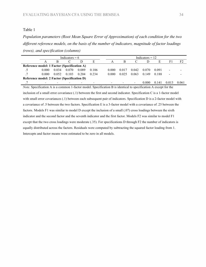
Table 1
Population parameters (Root Mean Square Error of Approximation) of each condition for the two
different reference models, on the basis of the number of indicators, magnitude of factor loadings
(rows), and specification (columns)
Indicators = 6 Indicators = 12 A B C D E A B C D E F1 F2 Reference model: 1 Factor (Specification A)
.5 0.000 0.034 0.070 0.089 0.106 0.000 0.017 0.042 0.070 0.091 - -
.7 0.000 0.052 0.103 0.204 0.234 0.000 0.025 0.063 0.149 0.188 - - Reference model: 2 Factor (Specification D)
.7 - - - - - - - - 0.000 0.141 0.013 0.061 Note. Specification A is a common 1-factor model. Specification B is identical to specification A except for the
inclusion of a small error covariance (.1) between the first and second indicator. Specification C is a 1-factor model
with small error covariances (.1) between each subsequent pair of indicators. Specification D is a 2-factor model with
a covariance of .5 between the two factors. Specification E is a 3-factor model with a covariance of .25 between the
factors. Models F1 was similar to model D except the inclusion of a small (.07) cross loadings between the sixth
indicator and the second factor and the seventh indicator and the first factor. Models F2 was similar to model F1
except that the two cross loadings were moderate (.35). For specifications D through F2 the number of indicators is
equally distributed across the factors. Residuals were computed by subtracting the squared factor loading from 1.
Intercepts and factor means were estimated to be zero in all models.

EVALUATING BAYESIAN CFA USING THE BRMSEA 35
Table 2
Proportion of rejected models with 6 indicators of the first section, with the 1-factor model as
reference model, using a cut-off point for the 90% confidence interval and 90% posterior
probability intervals of the root mean square error of approximation (RMSEA) and Bayesian
RMSEA (BRMSEA) for the upper limit of .08 and for the lower limit of .05 and of .05 for the
posterior predictive p value and p-value for the Bayesian confirmatory factor analysis (CFA), with
diffuse priors, and frequentist (CFA)
Factor loadings = .5 Factor loadings = .7
N Model BRMSEA ppp RMSEA p BRMSEA ppp RMSEA p 50 A (ref) .92 .01 .90 .09 .90 .01 .90 .10
B .93 .01 .91 .11 .92 .01 .91 .13
C .96 .01 .95 .16 .98 .07 .98 .33
D .98 .02 .96 .20 1 .51 1 .84
E .95 .02 .96 .12 1 .61 1 .91
100 A (ref) .72 .01 .80 .07 .67 .01 .80 .07
B .78 .01 .83 .11 .79 .03 .87 .17
C .91 .05 .94 .23 .97 .20 .99 .52
D .96 .11 .97 .39 1 .95 1 1.00
E .94 .1 .98 .37 1 .99 1 1
250 A (ref) .08 .00 .36 .06 .07 .00 .34 .07
B .20 .02 .57 .18 .38 .08 .75 .35
C .66 .23 .90 .62 .96 .77 1.00 .95
D .84 .51 .97 .81 1 1 1 1
E .93 .68 1.00 .93 1 1 1 1
500 A (ref) 0 .01 .03 .08 0 .01 .50 .08
B .01 .08 .18 .31 .13 .31 1 .65
C .46 .69 .81 .90 .98 1.00 1 1
D .81 .93 .97 .99 1 1 1 1
E .97 1 1 1 1 1 1 1
1,000 A (ref) 0 .00 0 .07 0 .00 0 .06
B 0 .22 .00 .58 .02 .74 .20 .93
C .33 .99 .74 1.00 1.00 1 1 1
D .89 1 .99 1 1 1 1 1
E 1.00 1 1 1 1 1 1 1
5,000 A (ref) 0 0 0 .06 0 0 0 .06
B 0 1.00 0 1 .20 1 .10 1
C 1 1 1.00 1 1 1 1 1
D 1 1 1 1 1 1 1 1
E 1 1 1 1 1 1 1 1
10,000 A (ref) 0 .00 0 .04 0 0 0 .05
B 0 1 0 1 .33 1 .16 1
C 1 1 1 1 1 1 1 1
D 1 1 1 1 1 1 1 1
E 1 1 1 1 1 1 1 1
Note. RMSEA = root mean square error of approximation; BRMSEA = Bayesian root mean square error of
approximation; ppp = posterior predictive p value; p = p-value; ref = reference model.

EVALUATING BAYESIAN CFA USING THE BRMSEA 36
Table 3
Proportion of rejected models with 12 indicators of the first section, with the 1-factor model as
reference model, using a cut-off point for the 90% confidence interval and 90% posterior
probability intervals of the root mean square error of approximation (RMSEA) and Bayesian
RMSEA (BRMSEA) for the upper limit of .08 and for the lower limit of .05 and of .05 for the
posterior predictive p value and p-value for the Bayesian confirmatory factor analysis (CFA), with
diffuse priors, and frequentist CFA
Factor loadings = .5 Factor loadings = .7
N Model BRMSEA ppp RMSEA p BRMSEA ppp RMSEA p 50 A (ref) .00 .04 .82 .21 0 .03 .82 .22
B .00 .04 .84 .22 .00 .05 .85 .23
C .02 .09 .90 .31 .03 .17 .96 .45
D .04 .19 .96 .51 .74 .94 1 .99
E .09 .28 .98 .64 .99 1.00 1 1
100 A (ref) 0 .02 .25 .10 0 .02 .26 .10
B 0 .02 .30 .13 0 .04 .35 .17
C 0 .10 .56 .31 .01 .33 .86 .65
D .02 .42 .87 .71 .97 1 1 1
E .15 .76 .98 .93 1 1 1 1
250 A (ref) 0 .01 0 .08 0 .01 0 .08
B 0 .03 0 .13 0 .07 .00 .23
C 0 .38 .02 .66 0 .93 .51 .98
D .01 .97 .73 1.00 1 1 1 1
E .37 1 1.00 1 1 1 1 1
500 A (ref) 0 .01 0 .06 0 .00 0 .05
B 0 .07 0 .18 0 .23 .00 .42
C 0 .92 .01 .97 .05 1 .61 1
D .27 1 .88 1 1 1 1 1
E .98 1 1 1 1 1 1 1
1,000 A (ref) 0 .02 0 .06 0 .02 0 .06
B 0 .20 0 .41 0 .63 0 .84
C 0 1 .00 1 .47 1 .92 1
D .88 1 .99 1 1 1 1 1
E 1 1 1 1 1 1 1 1
5,000 A (ref) 0 .01 0 .05 0 .01 0 .05
B 0 1 0 1 0 1 0 1
C 0 1 0 1 1 1 1 1
D 1 1 1 1 1 1 1 1
E 1 1 1 1 1 1 1 1
10,000 A (ref) 0 .00 0 .05 0 .00 0 .05
B 0 1 0 1 0 1 0 1
C 0 1 0 1 1 1 1 1
D 1 1 1 1 1 1 1 1
E 1 1 1 1 1 1 1 1
Note. RMSEA = root mean square error of approximation; BRMSEA = Bayesian root mean square error of
approximation; ppp = posterior predictive p value; p = p-value; ref = reference model.
EVALUATING BAYESIAN CFA USING THE BRMSEA 37
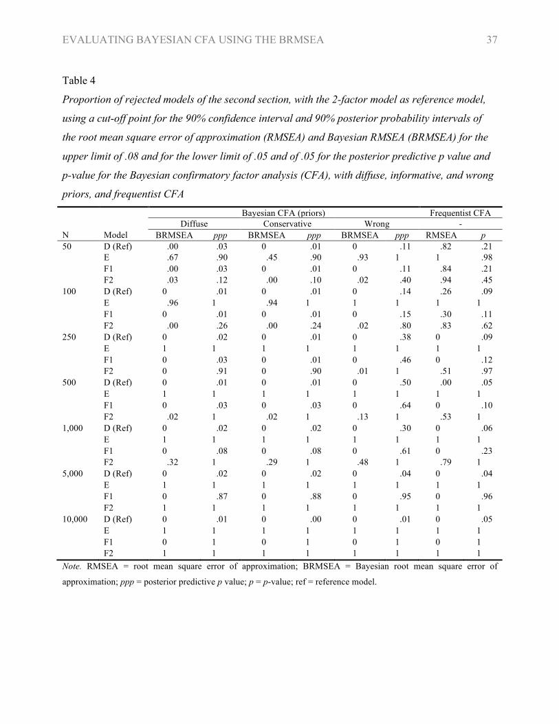
Table 4
Proportion of rejected models of the second section, with the 2-factor model as reference model,
using a cut-off point for the 90% confidence interval and 90% posterior probability intervals of
the root mean square error of approximation (RMSEA) and Bayesian RMSEA (BRMSEA) for the
upper limit of .08 and for the lower limit of .05 and of .05 for the posterior predictive p value and
p-value for the Bayesian confirmatory factor analysis (CFA), with diffuse, informative, and wrong
priors, and frequentist CFA
Bayesian CFA (priors) Frequentist CFA Diffuse Conservative Wrong - N Model BRMSEA ppp BRMSEA ppp BRMSEA ppp RMSEA p 50 D (Ref) .00 .03 0 .01 0 .11 .82 .21 E .67 .90 .45 .90 .93 1 1 .98 F1 .00 .03 0 .01 0 .11 .84 .21 F2 .03 .12 .00 .10 .02 .40 .94 .45 100 D (Ref) 0 .01 0 .01 0 .14 .26 .09 E .96 1 .94 1 1 1 1 1 F1 0 .01 0 .01 0 .15 .30 .11 F2 .00 .26 .00 .24 .02 .80 .83 .62 250 D (Ref) 0 .02 0 .01 0 .38 0 .09 E 1 1 1 1 1 1 1 1 F1 0 .03 0 .01 0 .46 0 .12 F2 0 .91 0 .90 .01 1 .51 .97 500 D (Ref) 0 .01 0 .01 0 .50 .00 .05 E 1 1 1 1 1 1 1 1 F1 0 .03 0 .03 0 .64 0 .10 F2 .02 1 .02 1 .13 1 .53 1 1,000 D (Ref) 0 .02 0 .02 0 .30 0 .06 E 1 1 1 1 1 1 1 1 F1 0 .08 0 .08 0 .61 0 .23 F2 .32 1 .29 1 .48 1 .79 1 5,000 D (Ref) 0 .02 0 .02 0 .04 0 .04 E 1 1 1 1 1 1 1 1 F1 0 .87 0 .88 0 .95 0 .96 F2 1 1 1 1 1 1 1 1 10,000 D (Ref) 0 .01 0 .00 0 .01 0 .05 E 1 1 1 1 1 1 1 1 F1 0 1 0 1 0 1 0 1 F2 1 1 1 1 1 1 1 1 Note. RMSEA = root mean square error of approximation; BRMSEA = Bayesian root mean square error of
approximation; ppp = posterior predictive p value; p = p-value; ref = reference model.

EVALUATING BAYESIAN CFA USING THE BRMSEA 38
Table 5 Summary of model acceptance, for each model specification and magnitude of the factor loadings, indicating if models were commonly accepted (+), rejected (-) or a mixed pattern emerged (0) for the conditions with a large sample size (N ≥ 1,000) with a cut-off point for the lower limit of .05 and for the upper limit of .08 for the 90% posterior probability intervals of the Bayesian root mean square error of approximation (BRMSEA) and 90% confidence interval of the RMSEA and of .05 for the posterior predictive p value and p-value Bayesian confirmatory factor analysis (CFA) Frequentist confirmatory factor analysis
(CFA) BRMSEA ppp RMSEA p-value
.5 .7 .5 .7 .5 .7 .5 .7 Reference model: 1 Factor (Specification A) A (ref) + + + + + + + + B + + 0 - + 0/+a 0 - C -/+a - - - -/+a - - - D - - - - - - - - E - - - - - - - - Reference model: 2 Factor (Specification D) D (ref) + +/0b + + E - - - - F1 + 0 + 0
F2 - - - - Conclusion (N ≥ 1,000)
Using the BRMSEA, models with no or “small” amounts of misspecification (e.g. B & F1) were generally accepted, whereas models with a “moderate” or “large” misspecification (e.g. E) were mostly rejected, irrespective if the reference model had one or two factors, if sample size increased. If factor loadings were smaller model acceptance became more liberal as models with a “large” misspecification were increasingly accepted. There were no noteworthy difference between priors (for large samples)
With increasing sample sizes the ppp rejects all models regardless the level of misspecification. Only a small proportion of models with a “small” amount of misspecification were accepted if the sample size was 1,000. These models were, however, always rejected if the sample size was 5,000 or 10,000. There were no noteworthy differences between priors (for large samples) except that some 2-factor reference models were rejected if the wrong prior specification was used. This effect diminished, however, in the largest sample sizes.
Using the RMSEA, models with no or “small” amounts of misspecification (e.g. B & F1) were generally accepted, whereas models with a “moderate” or “large” misspecification (e.g. E) were mostly rejected, irrespective if the reference model had one or two factors, if sample size increased. If factor loadings were smaller model acceptance became more liberal as models with a “large” misspecification were increasingly accepted.
With increasing sample sizes the χ2-test rejects all models regardless the level of misspecification. Some models with a “small” amount of misspecification were accepted if the sample size was 1,000. These models were, however, always rejected if the sample size was 5,000 or 10,000.
aModel acceptance differed for the number of indicators: the result for the 6 indicators was provided first, followed by the result for the 12 indicators. bModel acceptance differed for the different prior variations: the result for the diffuse and informative prior variations was provided first, followed by the result for the wrong prior variation. Note. If no superscripts are given no noteworthy differences were found for the different prior variations or the number of indicators and a joined summary was given. RMSEA = root mean square error of approximation; BRMSEA = Bayesian root mean square error of approximation; ppp = posterior predictive p value; ref = reference model.
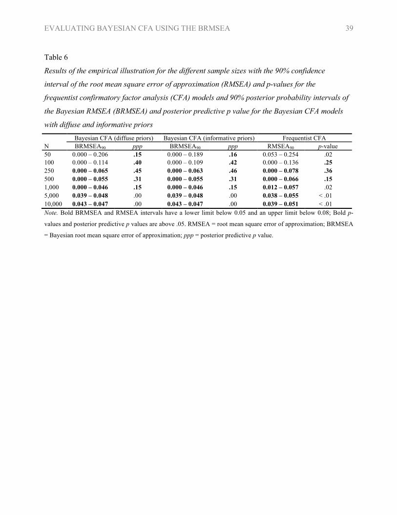
EVALUATING BAYESIAN CFA USING THE BRMSEA 39
Table 6
Results of the empirical illustration for the different sample sizes with the 90% confidence
interval of the root mean square error of approximation (RMSEA) and p-values for the
frequentist confirmatory factor analysis (CFA) models and 90% posterior probability intervals of
the Bayesian RMSEA (BRMSEA) and posterior predictive p value for the Bayesian CFA models
with diffuse and informative priors
Bayesian CFA (diffuse priors) Bayesian CFA (informative priors) Frequentist CFA N BRMSEA90 ppp BRMSEA90 ppp RMSEA90 p-value 50 0.000 – 0.206 .15 0.000 – 0.189 .16 0.053 – 0.254 .02 100 0.000 – 0.114 .40 0.000 – 0.109 .42 0.000 – 0.136 .25 250 0.000 – 0.065 .45 0.000 – 0.063 .46 0.000 – 0.078 .36 500 0.000 – 0.055 .31 0.000 – 0.055 .31 0.000 – 0.066 .15 1,000 0.000 – 0.046 .15 0.000 – 0.046 .15 0.012 – 0.057 .02 5,000 0.039 – 0.048 .00 0.039 – 0.048 .00 0.038 – 0.055 < .01 10,000 0.043 – 0.047 .00 0.043 – 0.047 .00 0.039 – 0.051 < .01 Note. Bold BRMSEA and RMSEA intervals have a lower limit below 0.05 and an upper limit below 0.08; Bold p-
values and posterior predictive p values are above .05. RMSEA = root mean square error of approximation; BRMSEA
= Bayesian root mean square error of approximation; ppp = posterior predictive p value.
EVALUATING BAYESIAN CFA USING THE BRMSEA 40
Figure 1. The different specifications for the population factor models used to generate the
population covariance matrices for each condition. Factor loadings (λi = .3, .5, or .7; λc = .07, .35)
and number of indicators (6 or 12) varied between the conditions. Residuals (θ) were computed on
the basis of the factor loadings (1 - λ2). Intercepts and factor means are not displayed as they were
estimated to be zero in all models. Model A through C were only used in the first section and
model F1 & F2 only in the second section. Model A was the reference model in the first section
and Model D was the reference model in the second section.
Figure 2. Mean values of the 500 replications for the 90% posterior probability interval (PPI) of
the Bayesian root mean square error of approximation (BRMSEA) and the posterior predictive p
value (ppp) for the Bayesian confirmatory factor analysis (CFA) models, both with informative
and diffuse priors, and for the 90% confidence interval (CI) RMSEA and p-value for the
frequentist CFA models of the first section, with the 1-factor model as reference (ref) model, for
each sample size (as ordinal variable) and specification condition in which the magnitude of the
factor loadings was .5. Cut-off values for the BRMSEA and RMSEA (.05 for the lower limit and
.08 for the upper limit) and for the posterior predictive p value and p-value (.05) are indicated with
the dashed lines. Values within these cut-off points have (blue) circles, those outside (red) squares
Figure 3. Mean values of the 500 replications for the 90% posterior probability interval (PPI) of
the Bayesian root mean square error of approximation (BRMSEA) and the posterior predictive p
value (ppp) for the Bayesian confirmatory factor analysis (CFA) models, both with informative
and diffuse priors, and for the 90% confidence interval (CI) RMSEA and p-value for the
frequentist CFA models of the first section, with the 1-factor model as reference (ref) model, for
each sample size (as ordinal variable) and specification condition in which the magnitude of the
factor loadings was .7. Cut-off values for the BRMSEA and RMSEA (.05 for the lower limit and
.08 for the upper limit) and for the posterior predictive p value and p-value (.05) are indicated with
the dashed lines. Values within these cut-off points have (blue) circles, those outside (red) squares
Figure 4. Mean values of the 500 replications for the 90% posterior probability interval (PPI) of
the Bayesian root mean square error of approximation (BRMSEA) and the posterior predictive p
value (ppp) for the Bayesian structural equation modelling (BSEM) models, both with informative,
diffuse, and wrong priors, and for the 90% confidence interval (CI) RMSEA and p-value for the

EVALUATING BAYESIAN CFA USING THE BRMSEA 41
frequentist CFA models of the second section, with the 2-factor model as reference (ref) model,
for each sample size (as ordinal variable) and specification condition. Cut-off values for the
BRMSEA and RMSEA (.05 for the lower limit and .08 for the upper limit) and for the posterior
predictive p value and p-value (.05) are indicated with the dashed lines. Values within these cut-
off points have (blue) circles, those outside (red) squares

EVALUATING BAYESIAN CFA USING THE BRMSEA 42
Figure 1

EVALUATING BAYESIAN CFA USING THE BRMSEA 43
Figure 2
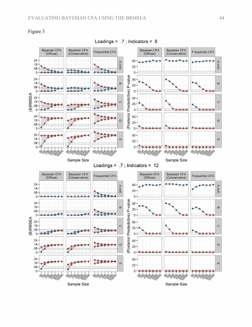
EVALUATING BAYESIAN CFA USING THE BRMSEA 44
Figure 3
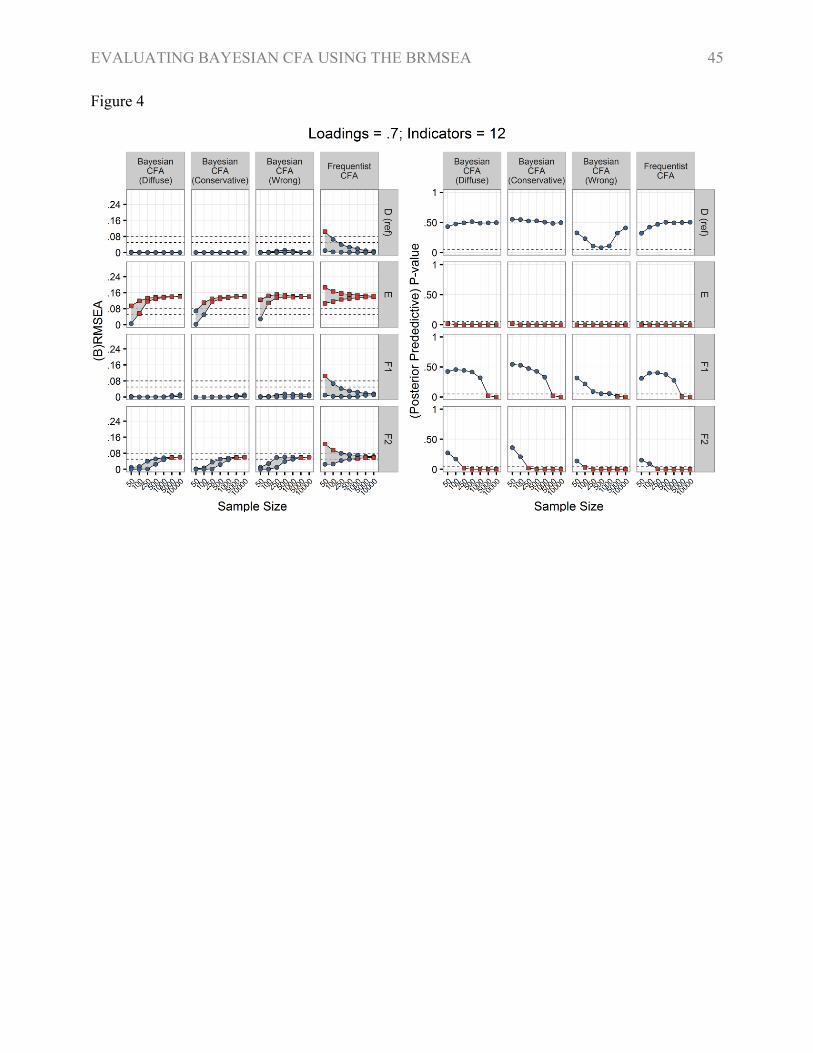
EVALUATING BAYESIAN CFA USING THE BRMSEA 45
Figure 4
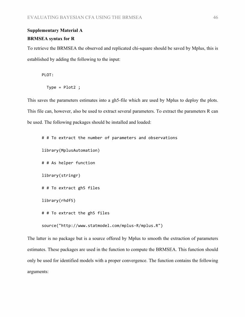
EVALUATING BAYESIAN CFA USING THE BRMSEA 46
Supplementary Material A
BRMSEA syntax for R
To retrieve the BRMSEA the observed and replicated chi-square should be saved by Mplus, this is
established by adding the following to the input:
PLOT:
Type = Plot2 ;
This saves the parameters estimates into a gh5-file which are used by Mplus to deploy the plots.
This file can, however, also be used to extract several parameters. To extract the parameters R can
be used. The following packages should be installed and loaded:
# # To extract the number of parameters and observations
library(MplusAutomation)
# # As helper function
library(stringr)
# # To extract gh5 files
library(rhdf5)
# # To extract the gh5 files
source("http://www.statmodel.com/mplus-R/mplus.R")
The latter is no package but is a source offered by Mplus to smooth the extraction of parameters
estimates. These packages are used in the function to compute the BRMSEA. This function should
only be used for identified models with a proper convergence. The function contains the following
arguments:

EVALUATING BAYESIAN CFA USING THE BRMSEA 47
• obs: A vector with the observed 𝜒I for each iteration
• rep A vector with the replicated 𝜒I for each iteration
• nvar Number of observed variables (positive integer)
• pD Effective number of estimated parameters (pD)
• N Sample size (N)
• ms Whether the mean structure is estimated (default = TRUE; ms included)
• cil Lower bound, proportion, of the posterior probability interval (default = .05; 5%)
• ciu Upper bound, proportion, of the posterior probability interval (default = .95; 95%)
• allout Whether the BRMSEA of each iteration should be provide or only the posterior
probability interval (default = FALSE)
• Min1 Whether to subtract 1 from the sample size in the equation (default = TRUE; yes)
• Ngr Number of groups (default = 1; one group; validity of BRMSEA for multiple
groups is not assessed, based on Steiger [1998; doi:10.1080/10705519809540115])
It is important that obs and rep have the same order in respect to the iterations they reflect. The
arguments, nvar, pD, and N, should only contain a single element. These arguments are used in
the following function to compute the BRMSEA:
BayesRmsea <-
function(obs, rep, nvar, pD, N, ms = TRUE, cil = .05,
ciu = .95, allout = FALSE, Min1 = TRUE, Ngr = 1){
# # Compute number of parameters
if(ms) p <- (((nvar * (nvar + 1)) / 2) + nvar)
if(!ms) p <- (((nvar * (nvar + 1))/ 2) + 0)

EVALUATING BAYESIAN CFA USING THE BRMSEA 48
p <- p * Ngr
# # Substract parameters and estimated parameters
dif.ppD <- p - pD
nonc <- ( ( obs-rep ) - dif.ppD )
# # Correct if numerator is smaller than zero
nonc[nonc < 0] <- 0
# # Compute BRMSEA (with or without the -1 correction)
if(Min1) BRMSEA <- sqrt(nonc / (dif.ppD * (N -1)))*sqrt(Ngr)
if(!Min1) BRMSEA <- sqrt(nonc / (dif.ppD * N ))*sqrt(Ngr)
# # Compute posterior probability intervals
BRMSEA_ci <- quantile(BRMSEA, probs = c(cil, ciu))
# # Save posterior probability interval or all BRMSEA
if(allout) out <- BRMSEA
if(!allout) out <- BRMSEA_ci
return(out)
}
Depending on the argument allout this function returns either the posterior probability
interval of the BRMSEA, or the BRMSEA for each iteration.
To extract the observed and replicated χ2, effective number of parameters (pD), and sample
size (N) from Mplus the following code can be used:
# # Retrieve observed and replicated chi-square

EVALUATING BAYESIAN CFA USING THE BRMSEA 49
file_sel <- "Chi-square values"
file <- "ModelName.gh5"
Obs <- mplus.get.bayesian.predictive.observed(file, file_sel)
Rep <- mplus.get.bayesian.predictive.replicated(file, file_sel)
# # Retrieve pD and N
sum <- extractModelSummaries(gsub("gh5", "out", file))
pD <- sum$pD
N <- sum$Observations
It has to be noted that Mplus and the default function of R extract quantiles in a slightly
different way. Using the credibility interval as given by Mplus to compute the 95% posterior
probability interval of the BRMSEA would therefore result in a slightly different outcome (often a
little wider).

EVALUATING BAYESIAN CFA USING THE BRMSEA 50
Supplementary Material B
Syntax for simulated models
This Appendix provides the syntax that is used to simulate and estimate the models. For an
automatization of this syntax see: http://git.io/vnInn. For more information about the syntax,
defaults, and model building see the manual of Mplus. As an example, only the condition with 6
indicators in which the sample size is 50 and factor loadings are .5 is given. The other condition
can be extracted from this example by changing the number of observations (sample size) or the
parameters of the models such as the factor loadings and number of indicators.
Model Simulation
The start for each model specification was the same.
TITLE:
Model; [Specification]
Sample Size; 50
Loadings; 0.5
Indicators; 6
MONTECARLO:
Names = y1-y6 ;
Nobs = 50 ;
Nreps = 500 ;
Save = file_*.txt ;
Repsave = 1-500 ;
Results = results.txt ;
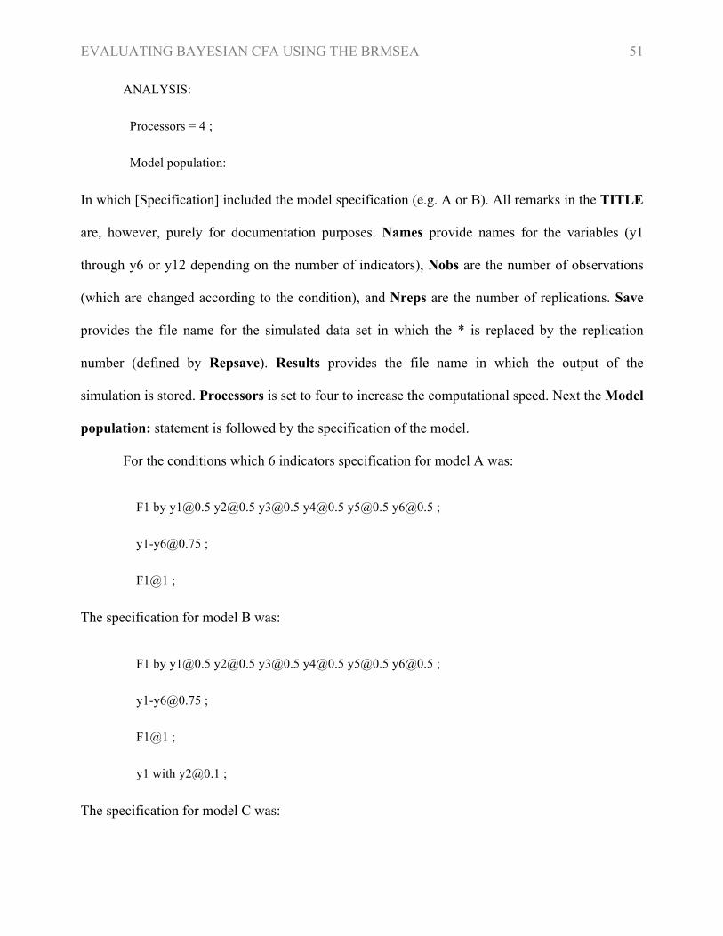
EVALUATING BAYESIAN CFA USING THE BRMSEA 51
ANALYSIS:
Processors = 4 ;
Model population:
In which [Specification] included the model specification (e.g. A or B). All remarks in the TITLE
are, however, purely for documentation purposes. Names provide names for the variables (y1
through y6 or y12 depending on the number of indicators), Nobs are the number of observations
(which are changed according to the condition), and Nreps are the number of replications. Save
provides the file name for the simulated data set in which the * is replaced by the replication
number (defined by Repsave). Results provides the file name in which the output of the
simulation is stored. Processors is set to four to increase the computational speed. Next the Model
population: statement is followed by the specification of the model.
For the conditions which 6 indicators specification for model A was:
F1 by [email protected] [email protected] [email protected] [email protected] [email protected] [email protected] ;
F1@1 ;
The specification for model B was:
F1 by [email protected] [email protected] [email protected] [email protected] [email protected] [email protected] ;
F1@1 ;
y1 with [email protected] ;
The specification for model C was:

EVALUATING BAYESIAN CFA USING THE BRMSEA 52
F1 by [email protected] [email protected] [email protected] [email protected] [email protected] [email protected] ;
F1@1 ;
y1 y3 y5 pwith [email protected] [email protected] [email protected] ;
The specification for model D was:
F1 by [email protected] [email protected] [email protected] ;
F2 by [email protected] [email protected] [email protected] ;
F1-F2@1 ;
F1 with [email protected] ;
The specification for model E was:
F1 by [email protected] [email protected] ;
F2 by [email protected] [email protected] ;
F3 by [email protected] [email protected] ;
F1-F3@1 ;
F1-F3 with F1-F3 @0.25 ;
Each of the model parameters is changed in accordance to the factor loadings. The intercept of
each indicator is 0 by default, as is the mean of each factor. Models with 12 indicators had the
same structure as only the number of indicators for each factor or factors differed.
The specification for model F1 was:
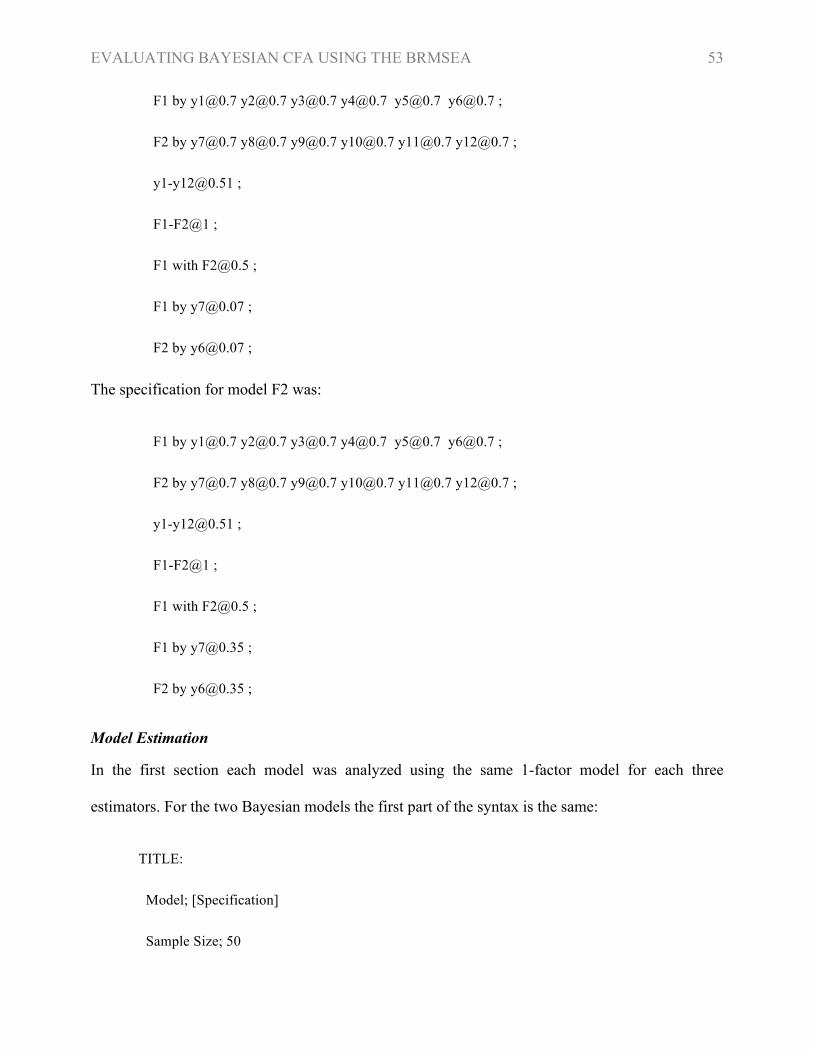
EVALUATING BAYESIAN CFA USING THE BRMSEA 53
F1 by [email protected] [email protected] [email protected] [email protected] [email protected] [email protected] ;
F2 by [email protected] [email protected] [email protected] [email protected] [email protected] [email protected] ;
F1-F2@1 ;
F1 with [email protected] ;
F1 by [email protected] ;
F2 by [email protected] ;
The specification for model F2 was:
F1 by [email protected] [email protected] [email protected] [email protected] [email protected] [email protected] ;
F2 by [email protected] [email protected] [email protected] [email protected] [email protected] [email protected] ;
F1-F2@1 ;
F1 with [email protected] ;
F1 by [email protected] ;
F2 by [email protected] ;
Model Estimation
In the first section each model was analyzed using the same 1-factor model for each three
estimators. For the two Bayesian models the first part of the syntax is the same:
TITLE:
Model; [Specification]
Sample Size; 50

EVALUATING BAYESIAN CFA USING THE BRMSEA 54
Loadings; 0.5
Indicators; 6
DATA:
File = file_[number].txt ;
VARIABLE:
Names = y1-y6 ;
ANALYSIS:
Estimator = BAYES ;
Processors = 8 ;
Chains = 8 ;
Biterations = 20000 (5000) ;
Bconvergence = .01 ;
MODEL:
F1 by y1-y6* (p1-p6) ;
[y1-y6*] (t1-t6) ;
F1@1 ;
PLOT:
Type = Plot2 ;
The [number] is replaced by the replication number (1-500). Names define the names and number
of variables. The names are the same as in the simulation (which is not a necessity). Estimator is
set to Bayes, Chains and Processors are both set to 8 to increase the computational speed. As
introduced in the method section of the manuscript the default values of the Bconvergence and

EVALUATING BAYESIAN CFA USING THE BRMSEA 55
Biterations are adapted to increase the likelihood of a model that has good convergence. The
Bconvergence is set to 0.01 which results in PSR values that are at least below 1.02. The minimal
number of iterations are set to 5000 and the maximum to 20000. Each model is specified
(estimated) as the specification A in the first section. The factor loadings are all freely estimated,
through *, and identification is achieved by setting the factor variance to 1, through @1. In a
default model, specification of the indicator intercepts is not necessary. If a prior is introduced,
however, it is required to specify the associated parameters in the model. These parameters are
labelled ((t1-t6)), as are the factor loadings ((p1-p6)), to be referred to when the priors are
specified. The factor mean is estimated by default at 0. The Plot2, resulting in a gh5-file, was
added to be able to extract the replicated and observed chi-square (see Appendix A). For the
models with 12 indicators, the number of variables was changed accordingly (y1-y12 instead of
y1-y6) also for the parameter labels.
The model with the conservative priors had the following additional lines in the model
statement:
Model priors:
p1-p6 ~ N(0.5, 0.05) ;
t1-t6 ~ N(0, 0.05) ;
The N indicates that the prior is normally distributed, the first number indicates the mean and the
second the variance of this (normal) prior distribution. The 0.5 is changed in accordance to the
factor loading, and the variance in accordance with the prior variation (e.g. 0.05).
The frequentist CFA model was estimated using the following syntax:
TITLE:
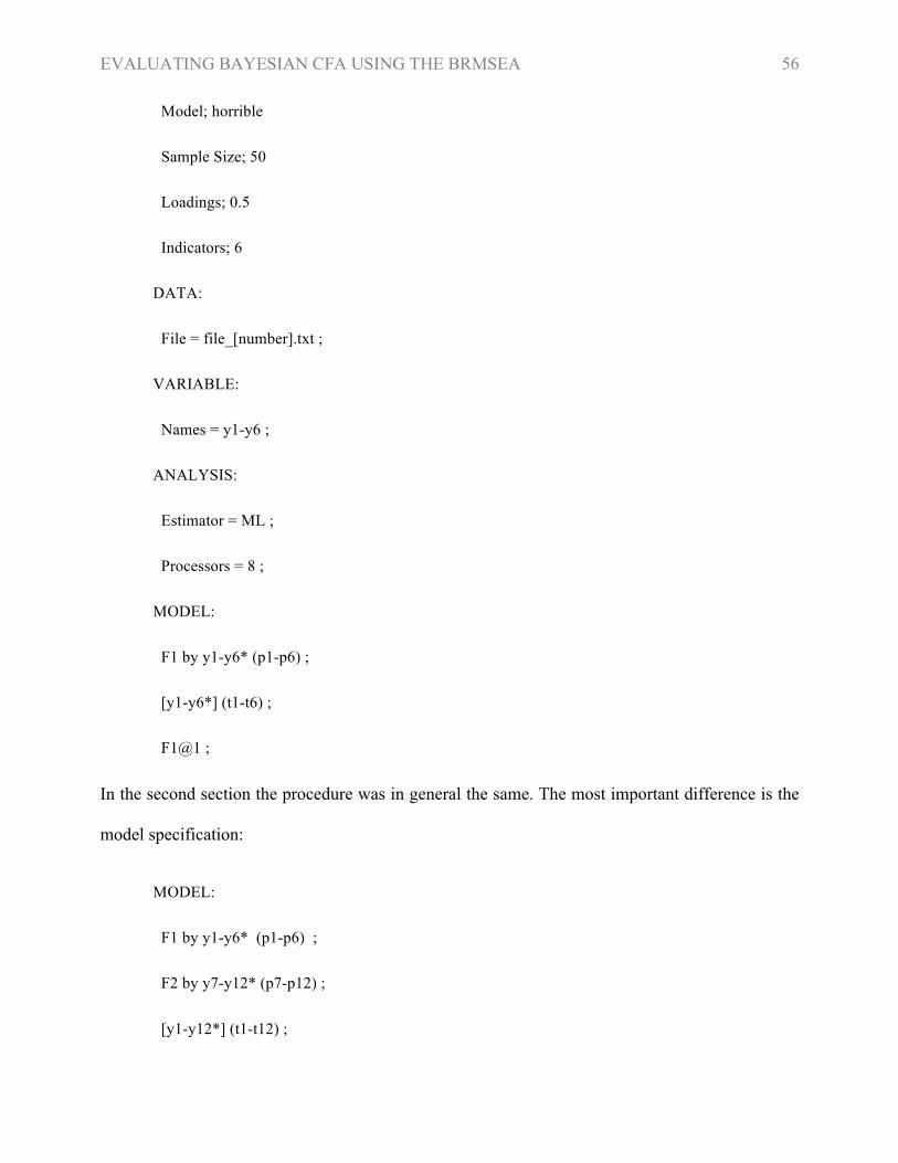
EVALUATING BAYESIAN CFA USING THE BRMSEA 56
Model; horrible
Sample Size; 50
Loadings; 0.5
Indicators; 6
DATA:
File = file_[number].txt ;
VARIABLE:
Names = y1-y6 ;
ANALYSIS:
Estimator = ML ;
Processors = 8 ;
MODEL:
F1 by y1-y6* (p1-p6) ;
[y1-y6*] (t1-t6) ;
F1@1 ;
In the second section the procedure was in general the same. The most important difference is the
model specification:
MODEL:
F1 by y1-y6* (p1-p6) ;
F2 by y7-y12* (p7-p12) ;
[y1-y12*] (t1-t12) ;

EVALUATING BAYESIAN CFA USING THE BRMSEA 57
F1@1 ;
F2@1 ;
F1 with F2 (F1corF2) ;
The other difference was the prior specification of the covariance in the conservative prior
variation:
Model priors:
p1-p12 ~ N(0.7, 0.05) ;
t1-t12 ~ N(0, 0.05) ;
F1corF2 ~ N(0.5, 0.05) ;
And in the wrong prior variation:
Model priors:
p1-p12 ~ N(0.9, 0.005) ;
F1corF2 ~ N(0.3, 0.005) ;
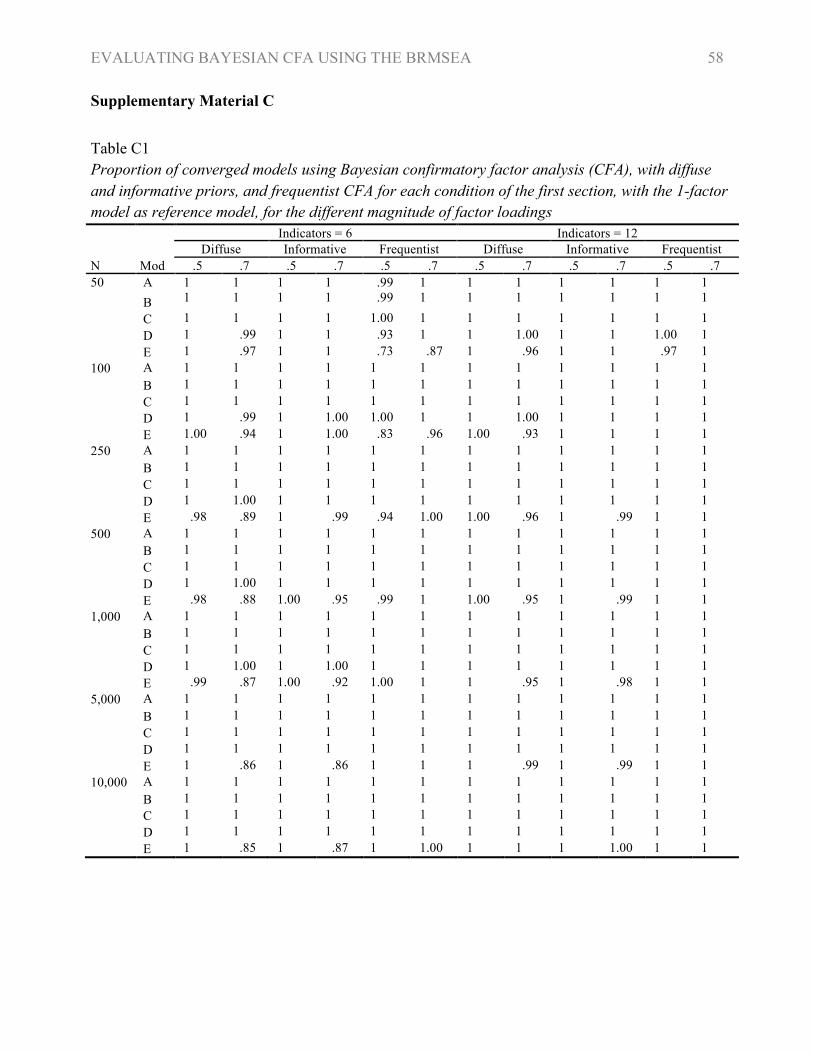
EVALUATING BAYESIAN CFA USING THE BRMSEA 58
Supplementary Material C
Table C1 Proportion of converged models using Bayesian confirmatory factor analysis (CFA), with diffuse and informative priors, and frequentist CFA for each condition of the first section, with the 1-factor model as reference model, for the different magnitude of factor loadings Indicators = 6 Indicators = 12
Diffuse Bayesian
Informative Bayesian
Frequentist CFA
Diffuse Bayesian
Informative Bayesian
Frequentist CFA N Mod
el .5 .7 .5 .7 .5 .7 .5 .7 .5 .7 .5 .7
50 A (ref)
1 1 1 1 .99 1 1 1 1 1 1 1
B 1 1 1 1 .99 1 1 1 1 1 1 1
C 1 1 1 1 1.00 1 1 1 1 1 1 1
D 1 .99 1 1 .93 1 1 1.00 1 1 1.00 1
E 1 .97 1 1 .73 .87 1 .96 1 1 .97 1 100 A
(ref) 1 1 1 1 1 1 1 1 1 1 1 1
B 1 1 1 1 1 1 1 1 1 1 1 1
C 1 1 1 1 1 1 1 1 1 1 1 1
D 1 .99 1 1.00 1.00 1 1 1.00 1 1 1 1
E 1.00 .94 1 1.00 .83 .96 1.00 .93 1 1 1 1 250 A
(ref) 1 1 1 1 1 1 1 1 1 1 1 1
B 1 1 1 1 1 1 1 1 1 1 1 1
C 1 1 1 1 1 1 1 1 1 1 1 1
D 1 1.00 1 1 1 1 1 1 1 1 1 1
E .98 .89 1 .99 .94 1.00 1.00 .96 1 .99 1 1 500 A
(ref) 1 1 1 1 1 1 1 1 1 1 1 1
B 1 1 1 1 1 1 1 1 1 1 1 1
C 1 1 1 1 1 1 1 1 1 1 1 1
D 1 1.00 1 1 1 1 1 1 1 1 1 1
E .98 .88 1.00 .95 .99 1 1.00 .95 1 .99 1 1 1,000 A
(ref) 1 1 1 1 1 1 1 1 1 1 1 1
B 1 1 1 1 1 1 1 1 1 1 1 1
C 1 1 1 1 1 1 1 1 1 1 1 1
D 1 1.00 1 1.00 1 1 1 1 1 1 1 1
E .99 .87 1.00 .92 1.00 1 1 .95 1 .98 1 1 5,000 A
(ref) 1 1 1 1 1 1 1 1 1 1 1 1
B 1 1 1 1 1 1 1 1 1 1 1 1
C 1 1 1 1 1 1 1 1 1 1 1 1
D 1 1 1 1 1 1 1 1 1 1 1 1
E 1 .86 1 .86 1 1 1 .99 1 .99 1 1 10,000 A
(ref) 1 1 1 1 1 1 1 1 1 1 1 1
B 1 1 1 1 1 1 1 1 1 1 1 1
C 1 1 1 1 1 1 1 1 1 1 1 1
D 1 1 1 1 1 1 1 1 1 1 1 1
E 1 .85 1 .87 1 1.00 1 1 1 1.00 1 1
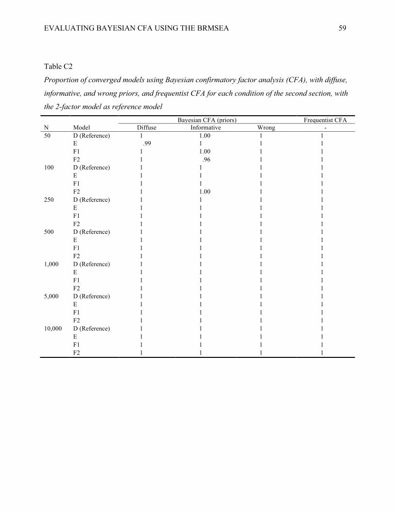
EVALUATING BAYESIAN CFA USING THE BRMSEA 59
Table C2
Proportion of converged models using Bayesian confirmatory factor analysis (CFA), with diffuse,
informative, and wrong priors, and frequentist CFA for each condition of the second section, with
the 2-factor model as reference model
Bayesian CFA (priors) Frequentist CFA N Model Diffuse Informative Wrong - 50 D (Reference) 1 1.00 1 1 E .99 1 1 1 F1 1 1.00 1 1 F2 1 .96 1 1 100 D (Reference) 1 1 1 1 E 1 1 1 1 F1 1 1 1 1 F2 1 1.00 1 1 250 D (Reference) 1 1 1 1 E 1 1 1 1 F1 1 1 1 1 F2 1 1 1 1 500 D (Reference) 1 1 1 1 E 1 1 1 1 F1 1 1 1 1 F2 1 1 1 1 1,000 D (Reference) 1 1 1 1 E 1 1 1 1 F1 1 1 1 1 F2 1 1 1 1 5,000 D (Reference) 1 1 1 1 E 1 1 1 1 F1 1 1 1 1 F2 1 1 1 1 10,000 D (Reference) 1 1 1 1 E 1 1 1 1 F1 1 1 1 1 F2 1 1 1 1