Evaluating Non-EU Models

Michael H. BirnbaumFullerton, California, USA

Outline

• This talk will review tests between Cumulative Prospect Theory (CPT) and Transfer of Attention eXchange (TAX) models.

• Emphasis will be on experimental design; i.e., how we select the choices we present to the participants.

• How not to design a study to contrast with how one should devise diagnostic tests.

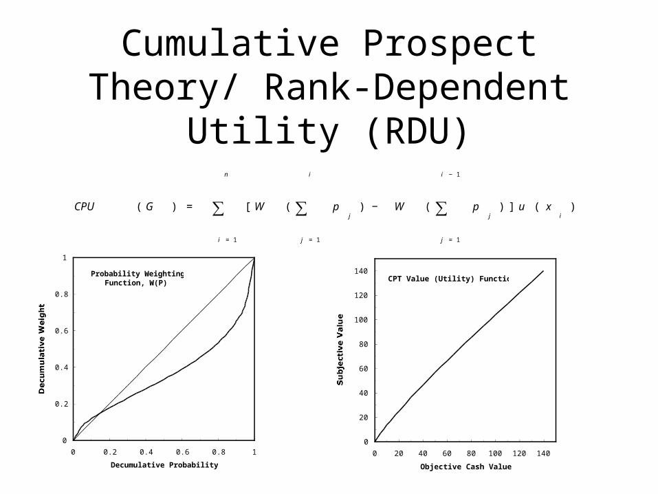
Cumulative Prospect Theory/ Rank-Dependent Utility

(RDU)

Probability Weighting Function, W(P)

0

0.2

0.4

0.6

0.8

1

0 0.2 0.4 0.6 0.8 1

Decumulative Probability

Decumulative Weight

CPT Value (Utility) Function

0

20

40

60

80

100

120

140

0 20 40 60 80 100 120 140

Objective Cash Value

Subjective Value

Nested Models

Testing Nested Models

• Because EV is a special case of EU, there is no way to refute EU in favor of EV.

• Because EU is a special case of CPT, there is no way to refute CPT in favor of EU.

• We can do significance tests and cross-validation. Are deviations significant? Do we improve prediction by estimating additional parameters (Cross-validation)? (It can easily occur that CPT fits significantly better but does worse than EU on cross-validation.)

Indices of Fit have little Value in Comparing Models

• Indices of fit such as percentage of correct predictions or correlations between theory and data are often insensitive and can be misleading when comparing non-nested models.

• In particular, problems of measurement, parameters, functional forms, and “error” can make a worse model achieve higher values of the index.

Individual Differences

• If some individuals are best fit by EV, some by EU, and some by CPT, we would say CPT is the “best” model because all participants can be fit by the same model.

• But with non-nested models with “errors” it is likely that some individuals will appear “best” fit by a “wrong” model.

“Prior” TAX Model

Assumptions:

€

U(G) =Au(x) + Bu(y) + Cu(z)

A + B + C

€

A = t( p) −δt(p) /4 −δt(p) /4

B = t(q) −δt(q) /4 + δt(p) /4

C = t(1− p − q) + δt(p) /4 + δt(q) /4

€

G = (x, p;y,q;z,1− p − q)

TAX Parameters

Probability transformation, t(p)

0

0.2

0.4

0.6

0.8

1

0 0.2 0.4 0.6 0.8 1

Probability

Transformed Probability

For 0 < x < $150u(x) = x Gives a decentapproximation.Risk aversion produced by

Non-nested Models

• Special TAX and CPT are both special cases of a more general rank-affected configural weight model, and both have EU as a special case, but neither of these models is nested in the other.

• Both can account for Allais paradoxes but do so in different ways.

How not to test among the models

• Choices of form: (x, p; y, q; z) versus (x, p; y’, q; z)EV, EU, CPT, and TAX as well as

other models all agree for such choices.

Furthermore, picking x, y, z, y’, p, and q randomly will not help.

Non-nested Models

CPT and TAX nearly identical inside the prob. simplex

How not to test non-EU models

• Tests of Allais types 1, 2, 3 do not distinguish TAX and CPT.

• No point in fitting these models to such non-diagnostic data.

• Choosing random levels of the gamble features does not add anything.

Testing CPT

• Coalescing• Stochastic

Dominance• Lower Cum.

Independence• Upper

Cumulative Independence

• Upper Tail Independence

• Gain-Loss Separability

TAX:Violations of:

Testing TAX Model

• 4-Distribution Independence

• 3-Lower Distribution Independence

• 3-2 Lower Distribution Independence

• 3-Upper Distribution Independence

CPT: Violations of:

Allais Paradox

• 80% prefer R = ($100,0.1;$7) over S = ($50, 0.15; $7)

• 20% prefer R’ = ($100, 0.9; $7) over S’ = ($100, 0.8; $50)

• This reversal violates “Sure Thing” Axiom. Due to violation of coalescing, restricted branch independence, or transitivity?

Decision Theories and Allais Paradox

Branch Independence

Coalescing Satisfied Violated

Satisfied EU, CPT*OPT*

RDU, CPT*

Violated SWU, OPT* RAM, TAX, GDU

C h o i c e d at a T AX C E

S R% R S R

1 5 r ed $ 5 0

8 5 bl ac k $ 7

1 0 bl ue $ 1 0 0

9 0 w hit e $ 7

8 0 * 1 4 < 1 8

1 0 r ed $ 5 0

0 5 bl ue $ 5 0

8 5 w hit e $ 7

1 0 bl ac k $ 1 0 0

0 5 p u r p l e $ 7

8 5 g ree n $ 7

4 9 1 6 > 1 5

8 5 r ed $ 1 0 0

1 0 w hit e $ 5 0

0 5 bl ue $ 5 0

8 5 bl ac k $ 1 0 0

1 0 y e ll ow $ 1 0 0

0 5 p u r p l e $ 7

6 3 * 6 8 < 7 0

8 5 bl ac k $ 1 0 0

1 5 y e ll ow $ 5 0

9 5 r ed $ 1 0 0

0 5 w hit e $ 7

2 0 * 7 6 > 6 2

Stochastic Dominance

• This choice does test between CPT and TAX

(x, p; y, q; z) vs. (x, p – q; y’, q; z)Note that this recipe uses 4 distinct

values of consequences. It falls outside the probability simplex defined on three consequences.

Basic Assumptions

• Each choice in an experiment has a true choice probability, p, and an error rate, e.

• The error rate is estimated from (and is the “reason” given for) inconsistency of response to the same choice by same person over repetitions

One Choice, Two Repetitions

A B

A

B€

pe2

+ ( 1 − p )( 1 − e )2

p ( 1 − e ) e + ( − p )( − e ) e

p ( 1 − e ) e + ( − p )( − e ) e

€

p ( 1 − e )2

+ ( 1 − p ) e2

Solution for e

• The proportion of preference reversals between repetitions allows an estimate of e.

• Both off-diagonal entries should be equal, and are equal to:

( 1 − e ) e

Estimating eProbability of Reversals in Repeated Choice

0

0.1

0.2

0.3

0.4

0.5

0 0.1 0.2 0.3 0.4 0.5

Error Rate (e)

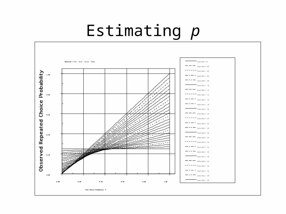
Estimating p

Observed = P(1 - e)(1 - e)+(1 - P)ee

0.00

0.20

0.40

0.60

0.80

1.00

0.00 0.20 0.40 0.60 0.80 1.00

True Choice Probabiity, P

Error Rate = 0

Error Rate = .02

Error Rate = .04

Error Rate = .06

Error Rate = .08

Error Rate = .10

Error Rate = .12

Error Rate = .14

Error Rate = .16

Error Rate = .18

Error Rate = .20

Error Rate = .22

Error Rate = .24

Error Rate = .26

Error Rate = .28

Error Rate = .30

Error Rate = .32

Error Rate = .34

Error Rate = .36

Error Rate = .38

Error Rate = .40

Error Rate = .42

Error Rate = .44

Error Rate = .46

Error Rate = .48

Error Rate = .50

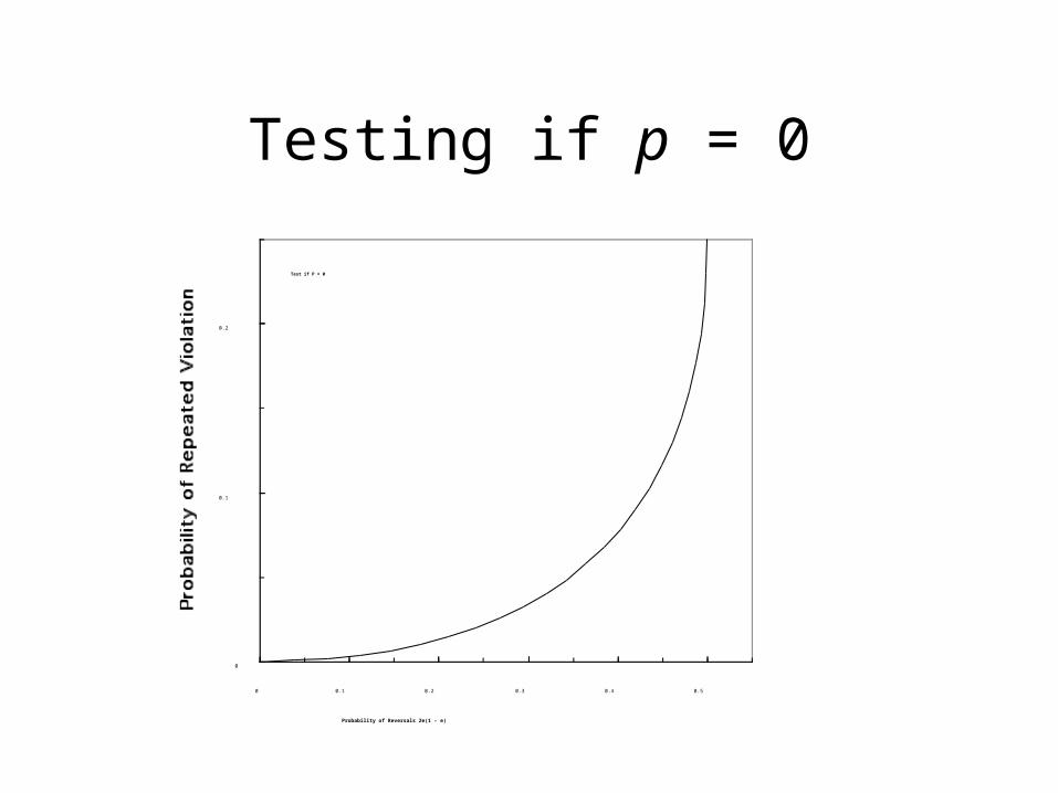
Testing if p = 0

Test if P = 0

0

0.1

0.2

0 0.1 0.2 0.3 0.4 0.5

Probability of Reversals 2e(1 - e)

Ex: Stochastic Dominance

: 05 tickets to win $12

05 tickets to win $14

90 tickets to win $96

B: 10 tickets to win $12

05 tickets to win $90

85 tickets to win $96

122 Undergrads: 59% repeated viols (BB) 28% Preference Reversals (AB or BA) Estimates: e = 0.19; p = 0.85170 Experts: 35% repeated violations 31% Reversals Estimates: e = 0.196; p = 0.50 Chi-Squared test reject H0: p < 0.4

Results: CPT makes wrong predictions for all 12 tests

• Can CPT be saved by using different participants? Not yet.

• Can CPT be saved by using different formats for presentation? More than a dozen formats have been tested.

• Violations of coalescing, stochastic dominance, lower and upper cumulative independence replicated with 14 different formats and thousands of participants.

Implications

• Results are quite clear: neither PT nor CPT are descriptive of risky decision making

• TAX correctly predicts the violations of CPT; several predictions made in advance of experiments.

• However, it might be a series of lucky coincidences that TAX has been successful. Perhaps some other theory would be more accurate than TAX. Luce and Marley working with GDU, a family of models that violate coalescing.