evaluating partisan gerrymandering in wisconsinis computed using votes from either the wisconsin...

Evaluating Partisan Gerrymandering in WisconsinGregory Herschlaga,b, Robert Raviera, and Jonathan C. Mattinglya,c

aDepartment of Mathematics, Duke University, Durham NC 27708; bDepartment of Biomedical Engineering, Duke University, Durham NC 27708; cDepartment of StatisticalScience, Duke University, Durham NC 27708

We examine the extent of gerrymandering for the 2010 General As-sembly district map of Wisconsin. We find that there is substantialvariability in the election outcome depending on what maps are used.We also found robust evidence that the district maps are highly ger-rymandered and that this gerrymandering likely altered the partisanmake up of the Wisconsin General Assembly in some elections. Com-pared to the distribution of possible redistricting plans for the Gen-eral Assembly, Wisconsin’s chosen plan is an outlier in that it yieldsresults that are highly skewed to the Republicans when the statewideproportion of Democratic votes comprises more than 50-52% of theoverall vote (with the precise threshold depending on the electionconsidered). Wisconsin’s plan acts to preserve the Republican ma-jority by providing extra Republican seats even when the Democraticvote increases into the range when the balance of power would shiftfor the vast majority of redistricting plans.

Gerrymandering | Redistricting | Monte Carlo Sampling | Wisconsin General Assembly

We generate an ensemble of 19,184 redistricting plans drawnfrom a distribution placed on redistricting plans of the state

of Wisconsin. The probability distribution used is concentrated onredistricting plans that satisfy design criteria laid out in the Wisconsinconstitution, statutes, and relevant court cases: compactness andcontiguity of districts, equal partition of votes, resistance to splittingcounties across districts, and compliance with the Voting Rights Act(VRA). With the possible exception of satisfying the VRA, none ofthese design criteria have any partisan tilt.

We explore three basic questions: the variability of elections re-sults across redistricting plans; the degree to which the Wisconsin Act43 is typical or an outlier with respect to its partisan bias; and lastly,the structural source of any bias.

Our approach has a number of inherent advantages. We do notpresume any notion of proportional representation based on statewidevote counts. By sampling, we are able to factor in the inherent geopo-litical structure of the state such as the concentration of Democratsin urban areas or the existence of geographic elements that constrainredistricting plans. Such features might produce basic asymmetries inthe number of representatives elected as a function of the statewidevotes. We make no symmetry assumptions and our methods naturallyadapt to the geometry of population distributions of the state.

In Section 1, we discuss how the election results may vary depend-ing on the restricting maps used. In Sections 2 and 3, we explore thegeopolitical structure of Wisconsin and give graphical aids for under-standing and detecting gerrymandering. In Section 4, we explore anumber of summary statistics which quantify the understanding andinsights developed in Sections 2 and 3.

We find that the Wisconsin redistricting plan is highly gerryman-dered and less representative than at least 99% of all plans in ourensemble and shows more Republican bias than over 99% of theplans. The gerrymandering results are stable over a number of differ-ent sets of votes and years. These results are summarized in Tables 1and 2 in Section 4. These results further suggest that the electionoutcomes produced by the Wisconsin maps systematically become

less representative of our ensemble as the overall percentage of Re-publican votes decreases to 50% and below. This is further supportedby graphical analysis in Figures 3–7 in Section 3. The Act 43 mapacts as a kind of firewall, keeping a Republican Assembly majorityin place even as voter preferences becomes increasingly Democratic.In Figure 9, we show that there is a fundamental asymmetry in thegeopolitical structure of Wisconsin as most of the redistricting mapsin our ensemble require less than 50% of the votes to be Republican tomake equal the chance of either party being in the legislative majority.Nonetheless, the Act 43 map is again a clear outlier in favor of theRepublicans as it requires a much lower percentage of Republicanvotes to produce an equal chance of having a legislative majority.

In Section 5, we discribe how the ensemble is generated by MarkovChain Monte Carlo. In Section 7, we give evidence that our results arerobust and that the algorithm is sufficiently converged. In particularwe show that the our all of our results remain unchanged when a largerensemble of 84,500 redistricting plans is used. In Sections 6 and 8,we make some technical comments about data curation.

This report continues our work started in (1–3). It is related toother works on sampling and computation in the redistricting context(4–11). In particular, the recent papers (12, 13) apply sampling to theWisconsin redistricting setting that we consider here.

1. The Inherent Variability of Election Results

For each redistricting plan in the ensemble, the outcome of the electionis computed using votes from either the Wisconsin General Assemblyelections from 2012 (denoted WSA12), from 2014 (denoted WSA16)and from 2016 (denoted WSA16). In all cases, the actual votes wereused at the ward level. However, the existence of unopposed racesnecessitated interpolating the data using votes from other electionsin a number of wards: 27% in WSA12, 46% in WSA14, and 49%in WSA16. The details of this interpolation are given in Section 6,but the vote counts are based on actual Wisconsin election data in theyears given.

Figure 1 shows the frequency of different election outcomes in ourensemble using the votes from WSA12, WSA14, and WSA16. Acrossthe redistricting plans for the 99-seat Wisconsin General Assembly,the expected number of seats won by Republicans was typically con-centrated within a range of 3-5 seats. However, a small proportion ofredistricting plans are outliers, which extend the range to as much as10 seats. This wide range of possible outcomes shows that the state’schoice of redistricting plan can have an effect on the same order asthe typical changes in the popular vote across elections (e.g. a swingof 60 to 64 elected Republicans from 2012 to 2016 in the WisconsinGeneral Assembly). The fact that the different redistricting plansin the ensemble give such different results speaks to the need for aconcept of acceptable redistricting, lest the state’s redistricting exer-cise become as, or more important than, the democratic expression ofvoters.

While the precise definition of a typical result may be debatable,

September 7, 2017 | 1–10

arX

iv:1

709.

0159

6v1

[st

at.A

P] 5

Sep

201

7

50 55 60 65 70 75

WSA12

Frac

tion

of re

sult

0

0.1

0.2

WSA14

Frac

tion

of re

sult

0

0.1

0.2

WSA16

Frac

tion

of re

sult

0

0.1

0.2

Elected Republicans50 55 60 65 70 75

Fig. 1. Distribution of election outcomes in the ensemble of 19,184 redistricting plans,interpolated for the WSA12, WSA14, and WSA16 election data. With a fixed numberand location of votes, the outcome of the election varies based on the choice ofredistricting plan chosen.

it is clear that some extreme ranges clearly represent anomalousbehavior: the results should be labeled as outliers. The view that somepoints would clearly be labeled as outliers is the starting point for ouranalysis.

2. Situating the Wisconsin Act 43 Redistricting in theEnsemble

We now turn to situating the actual redistricting plan established byAct 43 of the 2011 Wisconsin General Assembly within our ensembleof 19, 184 redistricting plans. This was the redistricting plan actuallyused in the WSA12, WSA14, and WSA16 elections. The annotation“WI” on each plot in Figure 2 indicates the number of seats producedby this redistricting. We note that the use of our modified electiondata in 2012 and 2014, which interpolates the missing data causedby unopposed races, does not change the balance of power. However,in 2016 the results of the actual election differed from those ourinterpolated vote data produces. The actual results had three fewerRepublican seats than the interpolated results would have had, due tounopposed races in which Democrats ran unopposed in districts thattended to vote Republican. The number of unopposed races was leastin 2012 with 27%, growing to 46% in 2014, and then to 49% in 2016.

Any reasonable sense of outlier would label the Wisconsin resultin 2012 as anomalous. Yet, the actual result produced by the samemap is well within the distribution for 2014 and 2016, in whichthe Republican share of the vote was considerably higher. As wesee below, this behavior turns out to reflects an unusual property ofWisconsin’s redistricting plan: it gives an anomalously high numberof seats to Republicans in elections in which Democrats performwell, but a typical number of seats in elections in which Republicansperform well.

To better understand this situation, we consider the outcome thatwould occur if votes from a number of other elections were used asif they had been cast for the Wisconsin General Assembly. Specifi-cally we compare the effect of using results from U.S. House, U.S.

WI

50 55 60 65 70 75

WSA12

Frac

tion

of re

sult

0

0.1

0.2

WI

WSA14

Frac

tion

of re

sult

0

0.1

0.2

WI (int)

WI (act)

WSA16

Frac

tion

of re

sult

0

0.1

0.2

Elected Republicans50 55 60 65 70 75

Fig. 2. Distribution of election outcomes in the ensemble of 19,184 redistricting plans,interpolated for the WSA12, WSA14, and WSA16 election data. The outcome usingthe Wisconsin Act 43 redistricting is marked with “WI”. For the WSA16 outcome, therewere three unopposed Democrats that ran in districts that voted more Republicanacross the interpolated data; thus we have marked the actual result (64), along withthe interpolated result (67).

Senate, and Presidential elections from 2012, 2014, and 2016 in ad-dition to our interpolated results for WSA12, WSA14, and WSA16.Figure 3 presents an interesting trend: whenever the election wouldhave typically produced around 55 or fewer Republican seats, theWisconsin plan behaves very anomalously in the sense that it is far tothe right in the histogram. In fact, even though the expected numberof Republican seats falls below 50 in one election and the statewidepercentage of Republican votes falls well below 50% in three elec-tions, the number of seats elected stays pinned in the high 50s; it isalmost constant despite the fact that the Republican vote continues tofall as one moves down the plot.

The plot shows that to determine whether the outcome of a givenmap will be anomalous for a particular election, it is not enough toconsider only the total vote count or expected number of seats. TheUSH12 and WSA12 are similar by those two metrics, yet the outcomein the first is typical but the second is anomalous. This detail showsthe importance of the geopolitical structure of the votes in determiningthe outcome and the pitfalls of coarse, global measures.

Based on these insights, we propose a method to evaluate theextent to which a state redistricting plan is an outlier with respect toits ability to protect a party from losing seats: we examine the impactof shifting the proportion of votes up or down within each electionexamined. We shift the proportions in WSA14 and WSA16 uniformlyup and down in all districts so that the statewide Republican votefraction varies from 45% to 55%. We then plot the histograms andthe election results for each shifted vote count in Figure 4.

Unlike the plots in Figure 3, the geopolitical structure of all ofthese shifted votes is identical. Both plots in Figure 4 exhibit the trendwe already observed in Figure 3. As the percentage of Republicanvotes decreases, the election results for both WSA14 and WSA16(shown with red dots in Figure 4) move from being representative

2 | Herschlag et al.

PRE12

USS12SOS14

USH12 WSA12

PRE16

WSA14

USH14

GOV14GOV12

WSA16

Frac

tion

of R

epub

lican

vot

e

0.46

0.48

0.50

0.52

0.54

Number of Republican seats 40 50 60 70

Fig. 3. A number of election seat result histograms situated on a larger plot by thenumber Republican seats and the overall fraction of Republican vote. The circlesmark the outcome using the Wisconsin Act 43 redistricting. Election plotted: Wis-consin State Assembly 2012 (WSA12), Wisconsin State Assembly 2016 (WSA16),Presidential 2012 (PRE12), Presidential 2016 (PRE16), US House 2012 (USH12),US House 2014 (USH14), US Senate 2012 (USS12), US Senate 2016 (USS16),Wisconsin Secretary of State 2014 (SOS14)

(located in the center of the histograms) to being outliers (located inthe extrema of the histograms).

The Wisconsin redistricting seems to create a firewall which resistsRepublicans falling below 50 seats. The effect is striking around themark of 60 seats where the number of Republican seats remainsconstant, despite the fraction of votes dropping from 51% to 48%.

Figure 5 gives a more stylized version of Figure 4. Rather than theentire histogram, we plot the mean, variance, a region containing 90%of all sampled redistricting plans, and the extrema for a larger numberof finer shifts that swing the election 10 percentage points in bothdirections of the observed result. The fine black line gives the numberof seats produced by the Wisconsin Act 43 redistricting. Though thelocal geography of the votes in the three elections is different, eachproduces a clear deviation from the typical results starting around50%. This deviation continues as the fraction of Republican votesdecreases. All three elections (especially WSA14 and WSA16) showa significant range of Republican votes where the partisan outcome ofthe election (expressed in the number of Republican seats) does notchange even though the percentage of the Republican votes decreasessubstantially.

Finally, we seek to summarize the extent to which Wisconsin’sredistricting plan is an outlier (compared to the ensemble of redistrict-ing plans). Toward this end, we defined a statistic as follows: for eachof various shifts around an equally split election, we (i) calculate theextent to which a state’s redistricting plan produces results differentfrom the results produced by the distribution of possible redistrictingplans, and (ii) take the average across the shifts. For any election, wethen measure the extent to which a state’s plan is outlier with respectto it statistic. (See Section 4 for more details.) As show in Figure 6,we find that the Wisconsin plan is an extreme outlier. In each of thethree elections (2012, 2014, and 2016), it is more extreme than 99% ofall possible redistricting plans in our ensemble (See the values ofH inTable 2 in Section 4). This statistic is essentially the log-likelihood ofseeing the election outcome produced in the Wisconsin plan averagedacross the shifted elections.

The above statistic is symmetric in that it measures if anomalousresults favors one political party over the other, not which party.Using a second set of statistics, we measure if one party is favoredover the other by the Wisconsin plan. For each party, we measure (i)

WSA16

Maj

ority

Supe

r Maj

ority

WSA14

Maj

ority

Supe

r Maj

ority

Republicans elected

Frac

tion

of R

epub

lican

vot

e

0.44

0.46

0.48

0.50

0.52

0.54

0.56

40 60 80 40 60 80

Fig. 4. The number of seats elected when the percentage in each district is shifted sothat the global fraction of the vote for the Republicans ranges between 0.45 and 0.55.Results of WSA14(left) and WSA16(right) are shown. Horizontal lines mark the levelof the original vote. Vertical lines mark the number of seats require for a majority anda super-majority.

what fraction of redistricting plans from our ensemble produce fewerlegislative seats than the state’s plan, and (ii) take the minimum ofthese fractions across all the shifts considered above. As before, forany election, we then measure the extent to which a state’s plan is anoutlier with respect to these statistics measuring party bias. In eachof the three elections (2012, 2014, and 2016), the Wisconsin plan ismore favorable to the Republicans with respect to this statistic than99% of all possible redistricting plans in our ensemble. In contrast,the percentage of plans that favor the Democrats less at some shift ismuch smaller (only 3%, 73%, and 8% in the 2012, 2014, and 2016elections respectively). See the values of Lrep and Ldem in Table 2 inSection 4). We will further see that, in the contexts in which the Act43 map aids Democrats, its effect is to make a large GOP majoritysomewhat smaller. In Section 7, we also consider a complementaryapproach in which we assess shifts of up to ±7.5% centered aroundthe outcomes of each election. Wisconsin’s plan is again seen to bean extreme outlier.

In the next section, we explain why the Wisconsin plan is suchan outlier by exploring the structure of the vote in more detail. Thegraphical understanding of the structure of the vote developed inthe next section, and Figure 7 in particular, is encapsulated in theGerrymandering Index defined in (3). In Section 4, we explore theGerrymandering Index of the Wisconsin plan over a number of histor-ical Wisconsin elections (WSA12, WSA14, WSA16, Governor 2012,US House 2012 and 2014, US Senate 2012 and 2016, WisconsinSecretary of State 2014, and Presidential 2012 and 2016). Againsituating the result in our ensemble, we fine that at worse 98% of ourensemble had a better Gerrymandering Index. For the majority of theelections considered, none of the redistrictings in our ensemble had aworst Gerrymandering score (See Table 1 in Section 1).

Herschlag et al. September 7, 2017 | 3

WSA12

Super Majority

Majority

Expected seatsWI (contested)Standard Deviation90% of ensembleBound

Num

ber o

f R

epub

lican

sea

ts

10

20

30

40

50

60

70

80

90

% Vote to the Republicans45 50 55 60

WSA14

Super Majority

Majority


Num

ber o

f R

epub

lican

sea

ts

20

30

40

50

60

70

80

90


WSA16

Super Majority

Majority


Num

ber o

f R

epub

lican

sea

ts

30

40

50

60

70

80

90


Fig. 5. Partisan composition of Wisconsin General Assemble as a function of globalRepublican vote using shifted WSA12(top), WSA14(middle), WSA16(bottom) votes.Vertical line indicates the actual votes in unshifted data. Horizontal lines mark seatsneeded for majority and super-majority. Thin line shows seats in Wisconsin redistrict-ing.

3. Exposing the Geopolitical Structure of Wisconsin

To understand the structure which leads to the results of the previoussection, we repeat the marginal analysis developed in (2, 3). Fixinga set of votes, for each redistricting we calculate the percentage ofRepublican votes and then place this vector of 99 numbers in increas-ing order. To gain insight into the distribution of this 99-dimensionalvector when varied over our ensemble, we plot a box-plot for eachmarginal direction. As standard in box-plots, the box contains 50%of the values, the outer whiskers bracket whichever is smaller – 1.5times the interquartile range from each quartile or the furthest outlier– and the central line through the box marks the median value.

The resulting 99 box-plots arranged on one graph for WSA12,WSA14, and WSA16 give insight into the inherent geopolitical geom-etry of Wisconsin due to the interaction of the state’s geometry withpopulation density and partisan distribution (Figure 7). We see thattypically there are at least 25 districts with less then 40% Democraticvote.

WI

WSA12

Probability

0

0.5

1.0

1.5

2.0

H1 2 3 4 5 6 7

WI

WSA14

Probability

0

0.5

1.0

1.5

2.0

H1 2 3 4 5 6 7

WI

WSA16

Probability

0

0.5

1.0

1.5

2.0

H1 2 3 4 5 6 7

Fig. 6. We plot the distribution of H indices, defined in Section 4, for each set ofvoting data. In all cases, we find that the Wisconsin Act 43 redistricting plan is anextreme outlier when compared with the ensemble.

These plots give provide a method to determine the typical partisanmakeup of each district. This inherently reflects the geopoliticalstructure of the state. For a given redistricting plan, if a given district’spercentage falls below the horizontal 50% line then the district electsa Republican. If it falls above the line, it elects a Democrat. Thisplot has proven useful in detecting redistricting plans with packed orfractured districts. See (3, 14). In some sense, they give quantitativedefinitions to these concepts.

If a given district’s Democratic vote percentage is at the bottom orbelow the box plot, the district has fewer Democrats than expected.If the percentage is above or at the top of the box plot, the districthas more Democrats than expected. It is clear that the WisconsinAct 43 redistricting plan produces election results with Democraticvotes depleted from the center of the plot and places those votes inthe districts which already have a large number of Democratic voters.

We also understand why the actual results of the WSA12 electionswere not representative while the actual results of the WSA14 andWSA16 elections were representative. It is simply a result of wherethe 50% line hits the box plot graph in Figure 7. If the 50% linecrosses the graph in the region in which the location of the currentWisconsin redistricting plan (the red dots) falls outside of the boxplot(which encodes typical behavior) then the results will be anomalous.This is the case in WSA12 but not in WSA 14 and WSA16. On theother hand, in all three years the district corresponding to the 50th seat,which dictates who is in the majority, is always an outlier, requiringless Republican votes than expected.

A. Inherent Lack of Proportionality. Notice that there is a struc-tural tilt to the Republicans – in all of our analyses, a 50% votefraction for both parties leads to a majority of Republicans. We seethat one only needs the Republican vote to be around 47% to 49%to obtain 50 seats with the structure of the WSA12 votes over the


WSA12

Frac

tion

of D

emoc

ratic

vot

e

0.2

0.3

0.4

0.5

0.6

0.7

0.8

0.9

District from most to least Republican0 10 20 30 40 50 60 70 80 90 100

0.40

0.45

0.50

0.5540 50 60

WSA14

Frac

tion

of D

emoc

ratic

vot

e

0.2

0.4

0.6

0.8

1.0


0.40

0.45

0.50

0.5540 50 60

WSA16

Frac

tion

of D

emoc

ratic

vot

e

0.2

0.3

0.4

0.5

0.6

0.7

0.8

0.9


0.40

0.45

0.50

0.5540 50 60

Fig. 7. Box-plot summary of districts ordered from most Republican to most Demo-cratic, for the voting data from WSA12 (top), WSA14 (middle), WSA16 (bottom). Wecompare our statistical results with Wisconsin redistricting in each case.

majority of redistricting plans. Similarly, WSA14 and WSA16 re-quire between 46% and 47% Republican vote fractions and between45% and 46% Republican vote fractions, respectively, to obtain 50seats. This shows clearly that it is not reasonable to expect that 50%of the vote leads to 50% of the seats. This does not explain all ofthe shift in the Republican favor produced by the Wisconsin Act 43redistricting plan. Our analysis allows us to separate out the effect ofthe geopolitical landscape, and to show that the Act 43 map generatesextreme partisan asymmetry above and beyond this effect.

B. Exploring Parity. To further explore the impact of the structurein Figures 5 and 7, we explore two ideas around parity. We begin byshifting the votes in WSA12, WSA14, and WSA16 so that there arean equal number of redistricting plans in the ensemble in which theRepublicans and Democrats are in the majority. When shifting thevotes in this way, the Wisconsin Act 43 redistricting produces signif-icantly more Republican seats – 56 with WSA12, 57 with WSA14,and 54 with WSA16. In the first two cases, this is a result seen in veryfew redistricting plans of the ensemble redistricting plans while inWSA16 it has a very low probability (that is to say a relatively smallnumber redistricting plans compared to the just under 20,000 plansconsidered in the ensemble).

Of course, one could perform a similar analysis around another

point than the 50% mark. One can see whether if the Wisconsinredistricting would still be an outlier when the votes are centeredaround a different line by drawing a vertical line in Figure 5 at adifferent value and noting where the thin black line correspondingto the Wisconsin Act 43 redistricting crosses this vertical line. Forinstance for WSA12, any vertical line up to at least 52% and above41% results in a result with Wisconsin Act 43 which is well outside theresults of 90% of the ensemble – very few redistricting plans whichgive this result exist in the ensemble. Similar in WSA14 from about43% to 50.5% the results produced by Wisconsin Act 43 are outliersas they lie outside the region containing 5% to 95% of the ensemble.Lastly for WSA16, from 42% to 50% the Wisconsin redistrictingproduces results which are outside the region containing 5% to 95%of the ensemble. In all cases the results are skewed to the Republicansprecisely in the region where the Democrats threaten to move into themajority.

WI

% o

f map

s

0

5

10

15

20

WSA12 Interpolated Votes (shifted to parity)40 45 50 55

WI

% o

f map

s

0

5

10

15

20


WI

% o

f map

s

0

5

10

15

20


Fig. 8. Histogram of Republican seats won when WSA12 (top), WSA14 (middle),WSA16 (botom) shifted so that half of the redistricting plans lead to a majority foreither party.

A complimentary perspective is instead to ask to what percentageof Republican vote does one have to shift the election to produce a50/50 split of the seats with a given redistricting. A histogram of thequantity tabulated over the ensemble is shown in Figure 9 along withthe percentage needed for the Wisconsin Act 43 redistricting plan.Again we see there is a systematic tilt towards the Republicans builtinto the geopolitical structure of the state. However, in all cases thepercentage needed to produce parity in the Wisconsin Act 43 plan isabnormally low.

4. Summary Statistics

We now develop a number of summary statistics that highlight andmake quantitative the graphical analysis developed in the last section.


WI

Prob

abilit

y

0

20

40

60

80

100

Republican vote needed for parity in election (2012)0.46 0.48 0.50

WI

Prob

abilit

y

0

50

100

Republican vote needed for parity in election (2014)0.44 0.46 0.48 0.50

WI

Prob

abilit

y

0

20

40

60

80

Republican vote needed for parity in election (2016)0.44 0.46 0.48

Fig. 9. Votes fraction needed so both parties have an equal chance at majority

Gerrymandering Index. We begin by calculating the GerrymanderingIndex developing in (3). It measures the extent to which a particularredistricting has districts whose vote margins for each election deviatefrom what is expected in Figure 7. For a given election, the square ofthe Gerrymandering index is the sum of the square deviations of eachof the sorted Democratic percentages from the means of the marginalsin the ninety-nine box-plots in Figure 7. To contextualize the Gerry-mandering Index, we situate a given score within the distribution ofscores from our ensemble of redistricting plans. Redistricting planswhich have unusually large Gerrymandering index should be view asGerrymandered. The percentage of the ensemble with Gerrymander-ing Index worst than the Wisconsin Act 43 redistricting is shown inTable 1 for a number of different sets of votes from different years.In all cases, the Wisconsin Act 43 redistricting is seen to have anunusually high level of the Gerrymandering Index.

Representative Index. The Gerrymandering Index directly measureshow anomalous the partisan composition of a redistricting is. It is pos-sible for a redistricting to be gerrymandered, yet still be representativeof the vote count, as we have seen in Figure 1 for WSA14 and WSA16.Therefore, we also measure how representative a redistricting is in thecontext of different vote counts.

In (3), we also define a Representative Index which quantifies howrepresentative the result obtained by using a particular redistrictingand vote combination is. It is essentially the distance from the meanvalue in the histograms in Figure 1 when one extends the number ofseats won by a given party to a continuous variable in a natural way.See (3) for the details. As with the Gerrymandering Index, in Table 1we postion the Representative Index inside the ensemble of redistrict-ing plans by reporting the percentage of the ensemble with a largerindex. It is worth noting that Table 1 shows the same dependenceof representativeness reflected in the histograms in Figures 3 and 4

Voting data % more gerry-mandered

% less represen-tative

Rep. VoteFraction.

WSA16 0.01 87.98 52.91GOV12 0 48.61 52.59USH14 0.09 46.78 51.89WSA14 0 82.34 51.28USS16 0 40.93 51.09WSA12 0 0.44 50.05PRE16 1.52 60.00 49.91USH12 0 25.02 48.68USS12 0 0 46.65PRE12 0 0 45.98

Table 1. We show the percentage of redistricting plans within theensemble that are (i) more gerrymandered and (ii) less representativethan Wisconsin Act 43 redistricting; we also display the republicanvote fraction. According to all vote counts, the current Wisconsinplan is highly gerrymandered. There is a strong correlation betweenRepublican vote fraction and Representativeness. (PRE = President,WAG=Attorney General, GOV= Governor, USS= US Senate, USH=USHouse)

and the plots in Figure 5. As the global percentage of Republicansdecreases towards 50% the representative score begins to drop. Theeffect is not strictly monotone as the geopolitical structure of eachvote also plays a role.

Representativeness Measured Across Shifts. From the preceding sec-tion, it is clear that the overall percentage of the vote as well as itsgeopolitical structure can have a large effect on the perceived rep-resentativeness of a redistricting, even when the GerrymanderingIndex reports a high level of gerrymandering. To control for this, weconsider shifts of a given collection of votes much in the spirit ofFigure 4.

Rather than use the Representative Index from (3), we consider analternative formulation which measures the negative log probabilityof the observed elevation outcome using the probabilities from ourensemble. We then sum these values over a number of shifts ofthe original election. The logarithmic measure more naturally liveson the same scale across different elections and hence seems moreappropriate for this context. This measure, which we will denote byH , is essentially an average log-likelihood across the different shifts

We compliment this nonpartisan statistic with one designed tomeasure deviations in the Republicans’s advantage, denoted by Lrep,and one to measure deviations in the Democrats’s advantage, denotedby Ldem. In Table 1, we see based on the H statistics that the Wiscon-sin Act 43 districts are outliers being much less representative thanmost of the redistricting plans in the ensemble. The L statistic showsthat the Wisconsin redistricting is tilted to favor the Republicans. Inone year the Ldem raises to the almost 75%; however the box-plotsin Figure 7 show that the benefit to Democrats comes in electionswhere the Republicans hold a strong majority in any event, so that thebenefit does not affect majority control.

To capture the representativeness over a range of election out-comes, we consider shifted election votes over a range of outcomes.We consider a measure which registers both the worst-case deviationfrom the typical and one which measures the average deviation.

Fixing a set of votes to evaluate election outcomes, we definethe index `rep to be the minimum, overall shifts of the percentageRepublican vote between 45% and 55%, of the probability that thenumber of Republican seats for a given map is greater than one drawn


from our distribution. We estimate this probability using the ensemblewe generated. We then define Lrep to be the fraction of maps in ourensemble for which `rep is greater than it is for the map in question.We define `dem and Ldem in the same fashion but with Republicansreplaced by Democrats.

The L statistics described above compare the worst case betweentwo redistricting plans and are inherently one-sided, hence the Demo-cratic and Republican versions. It is also useful to consider a statisticwhich is an average over a range of shifts. Again fixing a set of votesand a redistricting to be investigated, we define h to be the sum overa set of shifts of the logarithm of the probability that two of the redis-tricting plans in question produce the same number of Republicansas a random redistricting drawn from our distribution. As with thepreceding statistic, we determine a sense of scale for h by defining Hto be the probability that the h of a given redistricting is greater thana randomly drawn redistricting from our ensemble.

H Lrep Ldem

WSA12 100% 99.833% 3.253%WSA14 99.990% 99.765% 72.785%WSA16 99.223% 99.656% 7.892%

Table 2. Summary statistics measuring representativeness for Wis-consin Act 43 redistricting. These numbers give the percent of re-districting plans the Wisconsin Act 43 redistricting is worse than interms of average (H), Republican favoritism (Lrep), and Democraticfavoritism (Ldem).

The results in Table 2 show that the results are clearly anomalous.The values of H for the Wisconsin plan are extreme outliers withinour ensemble. By detecting unrepresentativeness over a range ofshifts, the H statistic assess the level of gerrymandering in the rangeof total vote fractions where elections typically occur.

We now clarify these definitions by restating them in more math-ematical notation. We begin by fixing some notation. For any redis-tricting π and s ∈ R, we let π + s to be the vote obtained by shiftingthe partisan vote s% to the Republicans. Let rep(π) and dem(π)denote respectively the total percent Republican or Democratic votein the election π. Now for any redistricting ξ, we let Rep(ξ, π) andDem(ξ, π) be the total number of seats won by respectively the Re-publicans and Democrats with vote π and redistricting ξ.

Now we define

`rep(ξ, π) = mins∈[45,55]−r(π)

P(

Rep(Ξ, π + s

)≥ Rep(ξ, π + s

))`dem(ξ, π) = min

s∈[45,55]−r(π)P(

Dem(Ξ, π + s

)≥ Dem

(ξ, π + s

))where Ξ is a redistricting chosen uniformly from our ensembleand [45, 55] − r(π) is compact notation for the set of shifts [45 −r(π), 55− r(π)]. We then situate these probabilities in the ensembleby defining

Lrep(ξ, π) = P(`rep(Ξ, π) ≤ `rep(ξ, π)

)Ldem(ξ, π) = P

(`dem(Ξ, π) ≤ `dem(ξ, π)

)where Ξ is again a randomly chosen redistricting from the ensemble.

To define the averaged representative index, we define the averagelog-likelihood

h(ξ, π) = − 1|I|

∑s∈I−r(π)

log P(

Rep(Ξ, π+s

)= Rep

(ξ, π+s

))

where Ξ is chosen according to our distribution on redistricting plansand I = {45, 45.5, . . . , 54.5, 55}, I − x is the shifted set defined asbefore by I − x = {y − x : y ∈ I}, and |I| is the number of pointsin I . We then situate these in the ensemble by defining

H(ξ, π) = P(h(ξ, π) ≥ h(Ξ, π)

).

In calculating H , we extrapolate the observed histogram using aGaussian tail approximation whenever a values is needed outside therange observed in the histogram.

We report the summary statistics in Table 2. We find that theWisconsin Act 43 redistricting is an extreme outlier in terms of howprobable it is to observe its value of H . We also find that in the worstcase, it can benefit the Republicans by more than 99% of all redis-tricting plans in our ensemble. Conversely, when shifting between45%-55% of the vote fraction, the Democrats are significantly im-peded in WSA12 and WSA16, and are aided to a much lesser degreein other elections and vote shifts. We remark that when we re-examineFigure 5, the Democrats are only ‘aided,’ once the Republicans haveobtained a super majority, as can be seen by the thin continuous linefalling below the 90% region.

5. Generating the Ensemble of Redistricting Plans

Our method begins by first placing a probability distribution on allthe reasonable redistricting plans. The probability distribution willbe concentrated on redistricting plans which better satisfy the designcertain specified in the laws and legal precedents covering redistrictingplans in Wisconsin. We then draw an ensemble of redistricting usingthe classical Markov Chain Monte Carlo algorithm. The frequency ofredistricting plans with different qualities will depend on how wellthose districts satisfy the design criteria.

A. The Distribution on Redistricting Plans. Following the pre-scription from (3) (see also (1, 14)), we consider distributions with adensity proportional to

e−βJ(ξ)

where ξ is the function which assigns to each ward a district which welabel with the numbers 1 to 99 for convenience. The score function Jwill be the sum of a number of different score functions

J(ξ) =wcompJcomp(ξ) + wpopJpop(ξ)+ wcountyJcounty(ξ) + wvraJvra(ξ)

where Jcomp(ξ) measures compactness, Jpop(ξ) measure populationdeviation from the ideal, Jcounty(ξ) the number of counties splitacross counties, and Jvra(ξ) measures the compliance with the VotingRights Act (VRA); the wi’s are positive weights. In all cases, lowscores will correspond to better compliance with the associated designcriteria.

We will use the population and compactness score functions from(3). The county and VRA score functions will versions of those from(3) with modifications to adapt to the details of the Wisconsin redis-tricting context. The Wisconsin State Assembly (WSA) districtingrequired that many counties and towns be split into more than twodistricts (in contrast to the work in (3)). Hence minor alterations wererequired to our previous score functions.

We determine the weight parameters with a nearly identical pro-cess to that described in (3). We have determined wpop = 2200,wcomp = 0.8, wcounty = 0.6, wV RA = 100.


B. Markov Chain Monte Carlo Sampling. We sample redistrictingplans according to the algorithm presented (3). For simulated anneal-ing parameters, we take 20,000 accepted steps at β = 0, 80,000accepted steps as β linearly increasing to one, and 20, 000 steps forβ = 1 ( see (3) for more details about the meaning of these pa-rameters). In our reported ensemble we take 19,184 samples. InSection 7, we show evidence that this is sufficient to correctly samplethe distribution on redistricting plans.

C. Redistricting Plans in the Ensemble. We ensure that the dis-tricts are contiguous, all redistricting plans are more compact than theWisconsin Act 43 plan. We only kept samples such that the maximumpopulation deviation is below 5%. To account for the VRA, we onlyretain redistricting plans containing six districts that have at least 40%African Americans and one district that has at least a 40% Hispanicpopulation. All sampled redistricting plans are described at the wardlevel, and no ward is split.

With the above criteria, we have account for all districting criteriapresent in the Wisconsin constitution, with the exception of splittingtownships. We also gather a smaller number of samples (2043) from adistribution that concentrates on redistricting plans that also preservetownships. The township consideration requires an additional term inthe score function, and is similar in form to the county splitting energy.We compare the effect of preserving townships below in Section 7.

6. Interpolating Election Data

We now explain how we interpolate the election data which is miss-ing due to unopposed races. Let Vtot(i), Vdem(i), and Vrep(i) berespectively the total vote, the Democratic vote, and the Republi-can vote in ward i. We split the ward indices into the good G andB wards. Typically the wards in B are the wards where the raceis unopposed. We also make use of a second set of voting data(Utot(i), Udem(i), Urep(i)) for which no data is missing. We beginby considering the pairs (Utot(i), Vtot(i)) : i ∈ {1, . . . 99}which weassume to be sorted by the first value. To interpolate Vtot(i) for somei ∈ B, we select the pairs{

(Utot(i−2), Vtot(i−2)), (Utot(i−1), Vtot(i−1)),

(Utot(i1), Vtot(i1)), (Utot(i2), Vtot(i2))}

where i1 and i2 are the next two elements in the increasing or-dered sequence of Utot values after Utot(i) so that i1, i2 ∈ G.Similarly Utot(i−2) and Utot(i−1) are the previous two elementsin the ordered sequence again so that both indices are in G. Ifno such point exists, we proceed with the points we have. Wethen perform a linear least-squares fit to this collection of points.Observe that there are always at least two points in the collec-tion. We then evaluate this linear fit at the point Utot(i) to obtainour estimate of Vtot(i) which we will denote by V̂tot(i). Then,in the same fashion, we estimate ρrep(i) = Urep(i)/Utot(i) andρdem(i) = Udem(i)/Utot(i) with rrep(i) = Vrep(i)/Vtot(i) andrdem(i) = Vdem(i)/Vtot(i) to obtain ρ̂rep(i) and ρ̂dem(i). Wethen set V̂rep(i) to be the average of floor(ρ̂rep(i)V̂tot(i)) andV̂tot(i))− ρ̂dem(i)V̂tot(i)) and similarly V̂dem(i) to be the averageof ρ̂dem(i)V̂tot(i) and V̂tot(i))− ρ̂rep(i)V̂tot(i). For each choice ofreference vote (Utot(i), Udem(i), Urep(i)), we obtain such an esti-mate. In some cases, we obtain multiple such estimates associatedwith different reference votes. We then average all of the estimates toobtain a finial estimate which we then round to the nearest integer.

To decide which of the many possible combinations of referencevotes (Utot(i), Udem(i), Urep(i)) produce the best results, we also

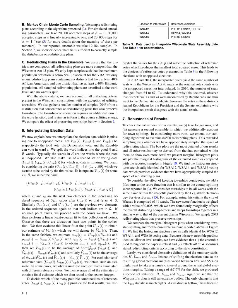
Election to interpolate Reference elections

WSA12 PRE12, USS12, USH12WSA14 GOV14, WAG14WSA16 PRE16, USS16

Table 3. Data used to interpolate Wisconsin State Assembly date.See Table 1 for abbreviations.

predict the values for the i ∈ G and select the collection of referencevotes which produces the smallest total squared error. This leads tothe choices of reference votes presented in Table 3 in the followingelections with unopposed elections.

In 2012 and 2014, the interpolated votes yield the same number ofseats with the Wisconsin Act 43 maps as the original vote counts withthe unopposed races not interpolated. In 2016, the number of seatschanged from 64 to 67. To understand why this occurred, observethat districts 54, 73 and 74 were uncontested by Republicans and thuswent to the Democratic candidate; however the votes in these districtsleaned Republican for the President and the Senate, explaining whythe interpolated result disagrees with the actual result.

7. Robustness of Results

To check the robustness of our results, we (i) take longer runs, and(ii) generate a second ensemble in which we additionally accountfor town splitting. In considering more runs, we extend our sam-pling algorithms to examine 84500 redistricting plans. This extendedsampling tests whether we have appropriately sampled the space ofredistricting plans. The box plots are the most detailed of our resultsand all other results may be derived from the data contained withinthem; to show even more detail we present marginal histogram plots.We plot the marginal histograms of the extended samples comparedwith the reported samples in Figure 10. We find the histogram struc-tures are visually identical for WSA12, WSA14, and WSA16 votingdata which provides evidence that we have appropriately sampled thespace of redistricting plans.

To consider the effect of keeping townships contiguous, we add afifth term to the score function that is similar to the county splittingscore reported in (3). We consider townships to be all wards with thesame name within the shapefile provided by the Legislative Technol-ogy Services Bureau (15). For example, using this criteria the city ofWausau is comprised of 41 wards. The new score function is weightedwith a value of 0.005, which we have found only marginally affectsthe overall districting compactness and keeps townships together in asimilar way to that of the current plan in Wisconsin. We sample 2043redistricting plans that preserve townships.

We compare the marginal histogram plots when considering town-ship splitting and for the ensemble we have reported above in Figure11. We find the histogram structures are visually identical for WSA12,WSA14, and WSA16 voting data. Because this new ensemble predictsidentical district level results, we have evidence that (1) the ensembleused throughout the paper is robust and (2) reflects all of Wisconsin’sstated redistricting criteria according to the state constitution.

Lastly, we considered alternative definitions of the summary statis-tics H , Lrep, and Ldem. Instead of shifting the election data so theresulting global elections margins varied between 45% and 55% onmight want to take a symmetric interval around the actual global elec-tions margins. Taking a range of ±7.5% for the shift, we produceda second set statistics: H̃ , L̃rep, and L̃dem. Again we see that theWisconsin’s plan is still an extreme outlier. The only change is thatthe L̃rep statistic is much higher. As we discuss bellow, this is because


Extended number of samplesReported Ensemble

Frac

tion

of D

emoc

ratic

vot

e

0.2

0.3

0.4

0.5

0.6

0.7

0.8

0.9

1.0

District from most to least Republican (WSA12)0 10 20 30 40 50 60 70 80 90 100

0.45

0.50

35 40 45 50 55

0.6

0.7

0.8

90 95


Frac

tion

of D

emoc

ratic

vot

e

0.2

0.4

0.6

0.8

1.0


0.40

0.45

35 40 45 50 55

0.60.70.80.9

90 95


Frac

tion

of D

emoc

ratic

vot

e

0.2

0.4

0.6

0.8

1.0


0.35

0.40

0.45

35 40 45 50 55

0.6

0.7

0.8

90 95

Fig. 10. Testing the effect of using an ensemble with more samples.

Accounting for township splittingReported Ensemble

Frac

tion

of D

emoc

ratic

vot

e

0.2

0.3

0.4

0.5

0.6

0.7

0.8

0.9

1.0


0.45

0.50

35 40 45 50 55

0.6

0.7

0.8

90 95


Frac

tion

of D

emoc

ratic

vot

e

0.2

0.4

0.6

0.8

1.0


0.40

0.45

35 40 45 50 55

0.60.70.80.9

90 95


Frac

tion

of D

emoc

ratic

vot

e

0.2

0.4

0.6

0.8

1.0


0.35

0.40

0.45

35 40 45 50 55

0.6

0.7

0.8

90 95

Fig. 11. Testing the effect of favoring townships not being split by district boundarieson the districting results.


H̃ L̃rep L̃dem

WSA12 100% 99.593% 73.718%WSA14 99.99% 99.505% 91.232%WSA16 97.795% 99.004% 87.484%

the range now includes a range of percentages where the Wisconsinplan causes the Democrats to perform better than expected in thetypical plan. However the results in this range have little effect onthe balance of power as the Republicans are already solidly in themajority in those elections.

We prefer H , Lrep, and Ldem to H̃ , L̃rep, and L̃dem because therange is limited to 45% to 55%. While the others are more symmetric,they often pull information from the low 60% or high 30% in globalvote. These ranges seem less relevant. The effect of this difference isseen in the values of L̃dem which is much higher than Ldem becausein includes elections with a large global percentage of Republicanvotes. From Figure 7, we see that the Democratic votes depletedfrom districts with partisen make up around 50% often is packedinto districts with more that 60%. This causes a tilt in favore of theDemocrats from what is expected should the global vote get that high.Of course if the vote is above 60% Republican, a few seats shifted tothe Democrats will have little effect operationally.

8. Adjustments to Wisconsin General Assembly Redis-tricting

Data provided in (15) is incomplete in terms of the current redistrictingplan for Wisconsin. We provide the script that we used to assigndistricts to unreported wards in our repository. The number of wardsaffected is relatively small.

9. Supplementary Materials

Database with redistricting plans and other data:[email protected]:gjh/WIRedistrictingData.git

10. Acknowledgements

This work uses a code base initiated by Han Sung Kang and JustinLuo as part of a Data+ project under the supervision of the authorsat Duke University. We thank the Information Initiative at Duke andthe Mathematics Department for their support. We would also liketo thank Moon Duchin, Assaf Bar-Natan, and Mira Bernstein fortheir guidance on districting criteria in Wisconsin and assistance withgathering and extracting data. We are also indebted to Eric Lander foruseful discussions and debates around the meaning and presentationof these results as well as Jordan Ellenberg’s insightful comments ona previous draft. We are also indebted to Venessa Barnett-Loro forhelping to polish this report.

1. Mattingly JC, Vaughn C (2014) Redistricting and the Will of the People. ArXiv e-prints.2. Tom Ross, POLIS center at Duke (2016) Beyond gerrymandering project (See

https://sites.duke.edu/polis/projects/beyond-gerrymandering/).3. Bangia S, et al. (2017) Redistricting: Drawing the Line. ArXiv e-prints.4. Thoreson JD, Liittschwager JM (1967) Computers in behavioral science. legislative districting

by computer simulation. Systems Research and Behavioral Science 12(3):237–247.5. Gearhart BC, Liittschwager JM (1969) Legislative districting by computer. Systems Research

and Behavioral Science 14(5):404–417.6. Wu LC, Dou JX, Sleator D, Frieze A, Miller D (2015) Impartial redistricting: A markov chain

approach. arXiv:1510.03247v1.7. Chen J, Rodden J (2015) Cutting through the thicket: Redistricting simulations and the detec-

tion of partisan gerrymanders. Election Law Journal 14(4):331–345.8. Liu YY, Cho WKT, Wang S (2016) Pear: a massively parallel evolutionary computation ap-

proach for political redistricting optimization and analysis. Swarm and Evolutionary Compu-tation 30:78–92.

9. Fifield B, Higgins M, Imai K, Tarr A (2015) A new automated redistricting simulator usingmarkov chain monte carlo. Work. Pap., Princeton Univ., Princeton, NJ.

10. Chikina M, Frieze A, Pegden W (2017) Assessing significance in a markov chain withoutmixing. Proceedings of the National Academy of Sciences 114(11):2860–2864.

11. Wang SSH (2016) Three tests for practical evaluation of partisan gerrymandering. StanfordLaw Review 68:1263–1322.

12. Chen J (2017) The impact of political geography on wisconsin redistricting: An analysis ofwisconsin’s act 43 assembly districting plan. Election Law Journal.

13. Chikina M, Frieze A, Pegden W (2017) An analysis of the Act 43 Wisconsin Assembly districtmap using the

√ε test. ArXiv e-prints.

14. Bangia S, Dou B, Mattingly JC, Guo S, Vaughn C (2015) Quantifying gerrymandering(https://services.math.duke.edu/projects/gerrymandering/).

15. (2017) Shape file web pages (http://data-ltsb.opendata.arcgis.com/datasets/2012-2020-wi-election-data-with-2017-wards). Last Modfied: 2017-08-31 00:23:26+0000.


[email protected]:gjh/WIRedistrictingData.git

http://data-ltsb.opendata.arcgis.com/datasets/2012-2020-wi-election-data-with-2017-wards

http://data-ltsb.opendata.arcgis.com/datasets/2012-2020-wi-election-data-with-2017-wards

evaluating partisan gerrymandering in wisconsinis computed using votes from either the wisconsin...

Documents