1

Evaluation and Comparison of Preliminary Meteorological Modeling for the August 2000 Houston-

Galveston Ozone Episode

John W. Nielsen-Gammon Department of Atmospheric Sciences

Texas A&M University

a report to the Technical Analysis Division, Texas Natural Resource Conservation Commission

February 5, 2002 Contact Information: John W. Nielsen-Gammon Department of Atmospheric Sciences 3150 TAMU College Station, TX 77843-3150 Phone: 979-862-2248 Fax: 979-862-4466

2

Summary This report is an evaluation of the quality of MM5 simulations of weather phenomena during the August 2000 Houston-Galveston Ozone episode. The report serves two purposes: first, to help guide final selection of a model configuration, and second, to evaluate the viability of MCNC’s real-time forecasting system as an alternative meteorological model for regulatory work. The TAMU and MCNC modeling efforts are both based on the MM5 model. Primary differences involve the incorporation of analysis information, the size of the domains, the boundary layer parameterizations, and the soil moisture specifications. Data used for the model evaluation include profiler data, surface meteorological data, radiosonde data, radar and satellite imagery, and doppler lidar data. The profiler and doppler lidar data sets are still evolving, and subsequent use of profiler data in this modeling effort will require consideration of both quality-controlled and non-quality-controlled data. The analysis of weather phenomena is conducted using the GEMPAK software package and TAMU-written converters and scripts. Overall, the TAMU simulations using the MRF PBL scheme (dec6grid4 and dec30grid4) performed best, with the Gayno-Seaman (dec16grid4) and MCNC simulations deficient in various critical errors. Precipitation was simulated remarkably successfully with the MRF PBL schemes; seven to eight days out of ten had no significant precipitation errors. The Gayno-Seaman run had the proper temporal variation but produced too much precipitation. The MCNC model did not properly simulate the squall line on August 24, produced rain in the wrong place on August 25, and failed to produce any rain at all on succeeding days. None of the model runs produced the observed outflow boundary on the evening of September 1, and all but the MCNC model produced an erroneous outflow boundary on the previous evening. Most clouds during the ozone episode were fair weather cumulus which formed at the top of the boundary layer in the morning and dissipated in late afternoon. None of the model runs can resolve these clouds, and as a result the models produce clouds with too large a horizontal extent. Under such circumstances, the simulation with the fewest clouds is usually the best, and in this case it was the runs with the MRF PBL scheme. None of the models had the proper day-to-day variations in cloudiness. The three TAMU runs had essentially zero maximum temperature bias, while the bias for the MCNC run was on the order of 3 C. This bias likely originates from the use of the default soil moisture. All model runs were able to track day-to-day temperature variations. It is recommended that temporally-varying soil moisture be used in subsequent model runs. Large-scale temperature patterns were generally forecasted well, except for the MCNC model in some cases. The land-sea contrast was well-simulated, except for MCNC, which had too small a contrast. Another major source of variability was the urban heat island, which during this episode was observed to be essentially nil during the day and significantly warmer than its surroundings at night. No model simulation produced a warm nighttime heat island, possibly because no simulation was able to get surrounding areas cool enough. Runs with relatively dry urban soil produce too strong a

3

daytime heat island; runs with relatively moist urban soil produce a late afternoon and evening urban “cool” island. Comparative analysis of soundings confirmed that the models’ nighttime temperature inversions were too weak or nonexistent. The MCNC runs were particularly deficient in that regard. During the day, it was found that the MRF PBL runs produced bias-free mixed-layer depths, while the Gayno-Seaman and MCNC simulations were too shallow by nearly 20% on average. Wind simulations on most days were good; frequently the wind field will evolve into a more accurate configuration as the model atmosphere responds to local forcing. A close look at August 25 and August 30 suggests that one or both might be successfully simulated with a photochemical model using the current, preliminary TAMU grids. The MCNC model had erroneously weak sea breeze winds because land areas were not heating up sufficiently. The vertical structure of the wind was dominated by a diurnally-varying component which seems to have large vertical extent on some days and very shallow extent on others. Further analysis of the diurnal wind cycle and the nocturnal low-level jet will be described in a subsequent report.

4

Table of Contents

List of Figures_________________________________________________ 5 List of Tables__________________________________________________ 9 1. Introduction_________________________________________________ 11 2. Model Configurations__________________________________________ 12 3. Data and Software_____________________________________________ 15 3a: Profiler data 15 3b: Sounding data 16 3c: Doppler lidar data 17 3d: Conventional data 17 3e: Analysis software 18 4. Day-by-day Weather Summary___________________________________ 19 4a: August 23 19 4b: August 24 19 4c: August 25 20 4d: August 26 20 4e: August 27 20 4f: August 28 21 4g: August 29 21 4h: August 30 22 4i: August 31 22 4j: September 1 22 5. Model Evaluation and Intercomparison____________________________ 24 5a: Precipitation 24 5b: Clouds 26 5c: Temperatures 27 5c1) Maximum and minimum temperatures 27 5c2) Surface temperature patterns 29 5c3) Thermodynamic profiles 32 5c4) Summary of model temperature performance 33 5d: Wind performance 34 5d1) August 25 34 5d2) August 30 36 5d3) Profiler commparisons 36 6. Conclusion__________________________________________________ 38 6a: TAMU Models 38 6b: MCNC Model 38 Figures________________________________________________________ 39

5

List of Figures

(figures appear consecutively in the back of this report) Figure 1: Horizontal extent of the TAMU 4 km domain (dark shading) and MCNC 5 km domain (embedded light shading). Figure 2: Locations of wind profiler sites and doppler lidar (LAP). Background is land use category from the TAMU 4 km grid. Figure 3: Vertical structure of low-level jet, 1200 UTC August 31 (blue) and 1200 UTC September 1 (pink), from doppler lidar data. Because of a malfunction of the lidar, the height of the data points is only known relative to the height of the wind maximum. The dashed black line is a linear extrapolation of the wind profile to the surface. Figure 4: Daily accumulated precipitation (cm), August 23-September 1, as simulated by the dec30grid4 model run. Note that two days are combined in the lower left panel. Figure 5: Daily accumulated precipitation (cm), August 23-September 1, as simulated by the dec30grid4 model run. Note that two days are combined in the lower left panel. Figure 6: Daily accumulated precipitation (cm), August 23-September 1, as simulated by the dec16grid4 model run. Note that two days are combined in the lower left panel. Figure 7: Daily accumulated precipitation (cm), August 23-September 1, as simulated by the MCNC model run. Note that two days are combined in the lower left panel. Figure 8: Incoming solar radiation (W/m2) and surface wind vectors (length equal to one-hour air parcel motion), dec6grid4 run, 2100 UTC August 24. Figure 9: Low-level reflectivity scan, Houston/Galveston WSR-88D doppler radar, 2102 UTC August 24, showing heavy rain (reds), light to moderate rain (greens and yellows), and outflow boundary (arc-shaped dark blue lines north and west of Houston). Figure 10: Incoming solar radiation (W/m2) and surface wind vectors (length equal to one-hour air parcel motion), dec30grid4 run, 2100 UTC August 24. Figure 11: Incoming solar radiation (W/m2) and lowest sigma level wind vectors (length equal to one-hour air parcel motion), MCNC run, 1500 UTC August 28. Figure 12: Incoming solar radiation (W/m2) and lowest sigma level wind vectors (length equal to one-hour air parcel motion), dec16grid4 run, 1500 UTC August 28. Figure 13: Incoming solar radiation (W/m2) and surface wind vectors (length equal to one-hour air parcel motion), dec30grid4 run, 1500 UTC August 28.

6

Figure 14: Visible satellite image, 1515 UTC 28 August. Figure 15: Maximum and minimum temperatures (C) during the August 2000 ozone episode at eight National Weather Service surface stations in the Houston/Galveston area, compared to 2 m temperatures simulated by the dec6grid4 and dec30grid4 model runs. Figure 16: Comparison of daily maximum and minimum temperatures at seven surface observing sites in the Houston-Galveston area, as simulated at 2 m and 17 m height above ground level by the dec30grid4 model run. Figure 17: Maximum and minimum temperatures at the 17 m level (TAMU runs) and 19 m level (MCNC run) at seven National Weather Service observing sites in the Houston/Galveston area during the ozone episode. Figure 18: Surface observations, 1500 UTC August 31. Temperatures (F) are blue, dewpoints (F) are green, ozone (ppbv) is white, winds (long barb = 10 kt) are yellow Figure 19: Surface (2 m) temperatures (F) and (10 m) winds, dec30grid4 model run, 1500 UTC August 31. Figure 20: Lowest sigma layer temperatures (F) and winds, dec16grid4 model run, 1500 UTC August 31. Figure 21: Surface (2 m) temperatures (F) and (10 m) winds, dec6grid4 model run, 1500 UTC August 31. Figure 22: Lowest sigma layer temperatures (F) and winds, MCNC model run, 1500 UTC August 31. Figure 23: Surface observations, 2100 UTC August 31. Figure 24: Surface (2 m) temperatures (F) and (10 m) winds, dec30grid4 model run, 2100 UTC August 31. Figure 25: Lowest sigma layer temperatures (F) and winds, dec16grid4 model run, 2100 UTC August 31. Figure 26: Surface (2 m) temperatures (F) and (10 m) winds, dec6grid4 model run, 2100 UTC August 31. Figure 27: Lowest sigma layer temperatures (F) and winds, MCNC model run, 2100 UTC August 31. Figure 28: Surface (2 m) temperatures (F) and (10 m) winds, dec6grid4 model run, 1500 UTC August 28.

7

Figure 29: Surface observations, 1500 UTC August 28. Figure 30: Lowest sigma level temperatures (F) and winds, dec16grid4 model run, 1500 UTC August 28. Figure 31: Surface weather observations, 2100 UTC August 28. Figure 32: Surface (2 m) temperatures (F) and (10 m) winds, dec30grid4 model run, 2100 UTC August 28. Figure 33: Vertical soundings of temperature (right, C) and dewpoint (left, C), 1100 UTC August 31, Wharton Power Plant (WPP). Maroon: observed. Orange: dec6grid4. Blue: dec30grid4. Green: dec16grid4. Magenta: MCNC. Observed wind vectors are plotted to the right. Figure 34: Vertical soundings of temperature and dewpoint, as in Fig. 33, but for 1100 UTC August 27. Figure 35: Vertical soundings of temperature and dewpoint, as in Fig. 33, but for 2000 UTC August 31. Figure 36: Surface weather observations, 1800 UTC August 25 Figure 37: Surface (2 m) temperatures (F) and (10 m) winds, dec6grid4 model run, 1800 UTC August 25. Figure 38: Lowest sigma level winds and temperatures, dec16grid4 model run, 1800 UTC August 25. Figure 39: Lowest sigma level winds and temperatures, MCNC model run, 1800 UTC August 25. Figure 40: Time-height cross section of observed onshore component of wind (toward 330 degrees) at HOU profiler site. Wind is contoured every 1 m/s with negative (toward sea) values dashed. The four panels, reading from left to right, begin at 1200 UTC August 24, 26, 28, and 30 and extend for 2 days and 6 hours, so that there is some overlap. The y axis is height above ground level, with grid lines every 200 m. Figure 41: Time-height cross section of coastline-normal wind, as in Fig. 40, but from dec6grid4 model output. Figure 42: Coastline-normal wind, as in Figs. 40 and 41, but from MCNC model output. Figure 43: Coastline-parallel wind, positive toward the northeast (30 degrees), from HOU consensus profiler observations. Plotting conventions as in Fig. 40.

8

Figure 44: Coastline parallel winds, as in Fig. 43, but from dec6grid4 model output. Figure 45: Coastline-parallel winds, as in Fig. 43, but from MCNC model output.

9

List of Tables Table 1: Comparison of vertical structure of the TAMU and MCNC model runs. Heights are given above ground level for the grid point closest to the Downtown Houston profiler/airsonde site. (page xxx) Table 2: Comparison of selected MM5 characteristics and settings. (page xxx) Table 3: Simulated and observed cloud cover during the ozone episode. 0 = no clouds, ISO = isolated clouds, SCT = scattered clouds (less than 50% coverage), BKN = broken clouds (more than 50% coverage), OVC = complete coverage. Clouds are mostly opaque unless otherwise specified as thin or med(ium). to S = to the south, to N = to the north. (page xxx) Table 4: Average pressure (hPa) at the top of the daytime PBL at Wharton Power Plant. (page xxx)

10

11

1. Introduction During fall and winter of 2001-2002, Texas A&M University (TAMU) is developing meteorological simulations for use by the Texas Natural Resource Conservation Commission (TNRCC) as drivers for photochemical model simulations of ozone development in the Houston-Galveston metropolitan area. The ozone episode being simulated is August 25-September 1, 2000, which occurred during the Texas 2000 Air Quality Study (TexAQS-2000). The special observations from the TexAQS-2000 field program provide an unprecedented data set for specification of the meteorological conditions during the ozone event. A description of the initial phase of the modeling work at TAMU is provided in the report dated December 19, 2001, and titled "Initial Modeling of the August 2000 Houston-Galveston Ozone Episode", available from TNRCC and at http://www.met.tamu.edu/results. This report will henceforth be referred to as Report 1.

During the field program, meteorological models, some coupled to photochemical models, were run in real time to provide meteorological and chemical forecasts to TNRCC and to the field program participants. One such model was run by the Microcomputer Center of North Carolina (MCNC). The ozone forecasts produced by this model were encouraging, and there is interest in knowing whether such a forecasting model can provide meteorological grids for regulatory purposes, even possibly as an alternative to the modeling being performed at TAMU.

The purpose of this report is twofold. First, we will compare the MCNC model forecasts to TAMU simulations of the same event, with particular emphasis on the ability of the forecasts and simulations to predict or reproduce the weather phenomena relevant to the formation and distribution of high concentrations of ozone in the Houston area, as those circumstances are presently understood. These key weather elements include cloud cover (or its absence), rain (or its absence), the existence and timing of periods of very light winds, and the wind distribution following periods of very light winds. In addition, such generic elements as planetary boundary layer (PBL) development and depth, temperatures, and the diurnal cycle of wind will be examined.

The second purpose of this report is to document and evaluate the performance of several of the TAMU model runs which are candidates for further development as simulations for use in photochemical modeling. This evaluation will help guide the selection of a specific model run as well as identify deficiencies in the model runs which may be addressed at a later date. In this report, we select three model runs and compare them to each other and to the MCNC forecasts.

12

2. Model Configurations The model used by TAMU is MM5, version 3.4. Two of the model runs (dec6grid4 and dec16grid4) were described in Report 1. Briefly, they are 4 km nested runs with soil moisture modifications made to the USGS 24-category land use characteristics in order to represent the drought characteristics present in the Houston area in late August 2000. A third model run (dec30grid4) was not described in Report 1 but is similar to the other two runs. All three model runs are continuous 10-day simulations, beginning at 1200 UTC (subtract six hours for CST), using Eta Data Assimilation System (EDAS) analysis for initial conditions, boundary conditions, and nudging on the 12 km nest which provides the one-way boundary conditions for the three runs described here. The analysis nudging constrains the 4-km model simulations to resemble reality, particular in their large-scale characteristics. The model used by MCNC is MM5, version 2.12. The inner nest, which is evaluated here, uses a 5 km grid spacing. The vertical grid spacing is also somewhat coarser, as shown in Table 1. In addition, the TAMU runs extend up to a nominal pressure of 50 hPa, while the MCNC runs extend only up to 100 hPa, so the TAMU runs have five additional levels in the upper troposphere and lower stratosphere. Unlike the TAMU runs, the MCNC runs are a series of consecutive 12-hour forecast runs. Each fine nest model run begins at 1100 UTC or 2300 UTC, eleven hours after the initiation of two coarser nests. The coarse nests use EDAS analyses (when available) for a three-hour dynamic initialization and the Eta model forecasts (when available) as lateral boundary conditions on the outer nest. Consequently, the MCNC model output is a sequence of 11 to 23 hour MM5 forecasts. This difference in setup has consequences for interpretation of the output. Most noticeably, the MCNC output will tend to have discontinuities at 1100 UTC and 2300 UTC each day, at the temporal boundaries between successive model runs. While this discontinuity is artificial, it does not necessarily imply a degradation of model accuracy. Effectively, the MCNC model run is updated with new weather information every twelve hours. The TAMU runs are updated continuously, but the information must propagate into the fine nest from the lateral boundaries. The MCNC fine nest is updated throughout its domain, although the information is at least eleven hours old. It is not immediately clear which technique would lead to more accurate simulations, all other things being equal. The answer depends on many factors, including the speed at which information penetrates the into the fine domain from its lateral boundaries and the relative accuracy of the MM5 forecasts compared to the EDAS analyses. It should also be noted that the MCNC forecasts, while rerun during the fall of 2001, were configured identically to the original forecast runs. More accurate model runs could have been produced at MCNC by using analyses instead of forecasts for lateral boundary conditions or by modifying the MM5 model configuration based on evaluation of model output. Thus, this evaluation is a comparison of the accuracy of the MM5 run in forecast mode to a set of refined MM5 retrospective simulations. A second potentially important difference between the two model runs is the size of the innermost domains (Fig. 1). The MCNC domain is much smaller than the TAMU domain. The MCNC domain is as small as possible so that the model can produce

13

forecasts quickly. Based on past Houston modeling experience, the inner domain boundaries will not seriously harm the solution beyond about seven grid points from the model boundaries. The simulations will also behave differently because the MCNC simulation in the Houston area is more sensitive to the characteristics of the coarser 15 km simulation; information from the coarse domain will reach Houston much more quickly in the MCNC run than in the TAMU runs. Other model configuration differences are relatively minor and are listed in Table 2. Taken as a whole, neither configuration is clearly preferable to the other. The soil moisture specification is described more completely in Report 1. The MCNC runs used the soil moisture availability specified in the land use file provided with the MM5 model. The TAMU dec6grid4 run used drier soil moisture for the land use categories common around Houston, except the urban category was left unchanged. This configuration was called “basic” soil moisture in Report 1. The other two TAMU runs used soil moisture availability set to .1 (lower than “basic”) in the land use Table 1: Comparison of vertical structure of the TAMU and MCNC model runs. Heights are given above ground level for the grid point closest to the Downtown Houston profiler/airsonde site.

TAMU level

TAMU height (m)

MCNC level

MCNC height (m)

43 20351 42 19322 41 18094 40 16904 39 15756 38 14651 31 14877 37 13589 30 13487 36 12568 29 12251 35 11586 28 11131 34 10577 27 10124 33 9615 26 9224 32 8746 25 8410 31 7953 24 7648 30 7267 29 6669 23 6915 28 6107 22 6223 27 5576 21 5579 26 5108 20 4977 25 4696 24 4300 19 4411 23 3919 18 3888 22 3553 17 3382 21 3199 20 2858 16 2891 19 2528 15 2432 18 2234 17 1975 14 2023 16 1722 13 1683 15 1475 12 1407 14 1282 13 1139 11 1181 12 998 10 994 11 859 9 844 10 745 8 712 9 645 8 565 7 582 7 476 6 453 6 388 5 300 5 326 4 214 4 212 3 128 3 127 2 59 2 65 1 17 1 19

14

Table 2: Comparison of selected MM5 characteristics and settings Model aspect TAMU runs MCNC runs Model version 3.4 2.12 Grid spacing 4 km (within 12, 36, and 108) 5 km (within 15 and 45) Vertical half-levels 43 31 Innermost nesting one-way one-way Radiation scheme RRTM Dudhia Radiation update frequency

30 min 10 min

Cumulus parameterization

Grell (none on fine nest) Kain-Fritsch (none on fine nest)

Cloud physics Simple ice Simple ice PBL scheme dec6grid4: MRF

dec16grid4: Gayno-Seaman dec30grid4: MRF

Blackadar

Soil scheme 5-layer 5-layer Shallow convection scheme

yes no

Coriolis force 3-d 2-d Soil moisture dec6grid4: drier than standard

dec16grid4: much drier than standard, except urban areas dec30grid4: much drier than standard, except urban areas

standard

Land use 25-category USGS 25-category USGS categories around Houston, and .2 (moister than standard to take into account urban irrigation) in the urban category. This configuration was called “dry” soil moisture in Report 1.

15

3. Data and Software The present evaluation focuses on the phenomena simulated by the modeling systems. The special observations taken during TexAQS-2000 are used to define the key phenomena of relevance to ozone formation and transport. In this section, we discuss the observational data and the tools used to compare the models and observations. Additional observational data, such as data from aircraft, was not utilized in this comparison due to pressing deadlines. 3a: Profiler data The most valuable data set consists of profiler data from the six profilers operated in the Houston-Galveston area during TexAQS-2000 (Fig. 2). These sites are: Houston Southwest Airport (HOU), UH Coastal Research Center at Lamarque (LAM), Ellington Field (ELL), Houston Downtown (HTN), Wharton Power Plant (TX2), and Liberty Municipal Airport (LMA). The profiler data has been quality-controlled in a four-step process by the Environmental Technology Laboratory (ETL) of the National Oceanographic and Atmospheric Administration. In the first step, the moments were examined to manually identify periods and elevations in which the signals were likely to be contaminated by migrating birds. In the second step, the data was sent through the Webber-Wuertz algorithm to compute the most representative wind speeds for each hour from the individual (typically) six-minute vertical scans. In the third step, the output was manually viewed at ETL and obviously erroneous data points were eliminated. In the fourth step, the data was viewed by John Nielsen-Gammon of TAMU and compared to profiler data prior to Webber-Wuertz processing, and additional suspicious data points were identified. These points were examined independently by ETL, and some of the points TAMU identified as suspicious were eliminated. This ETL work was performed by David White and Allen White. An alternative source of profiler data is the consensus data archived by NOAA’s Aeronomy Laboratory by Wayne Angevine. This data set has not been subjected to any quality control beyond what was done automatically when the data was recorded. A comparison of the two data sets indicates that the quality control has apparently eliminated all of the bird-contaminated data and has generated more coherent data, particularly at night or aloft. However, the Webber-Wuertz processing also tended to produce hourly observations that were inconsistent with observations at adjoining hours, while the consensus data was consistent from hour to hour. This tendency was most common within well-mixed daytime planetary boundary layers, but at least one profiler seemed unaffected (Liberty) and one profiler seemed affected throughout the day (Lamarque). The cause of this discrepancy is not known; perhaps the Webber-Wuertz algorithm is keying on successive observations of fragments of boundary-layer rolls or other boundary-layer circulations as they pass over the profiler sites. Whatever the cause, our extensive analysis of five of the profilers (we have not examined the Houston Downtown profiler data) suggests that the daytime observations are clearly improved by Webber-Wuertz at Liberty and clearly degraded by Webber-Wuertz at Houston Southwest. At the remaining three sites, the differences between the

16

two data sets are more substantial and the better of the two is not readily determined. Therefore, we utilize both sets of profiler data in our evaluation of the meteorological models. We retain the ETL bird masking in both data sets. Having both data sets provides some measure of the error bars associated with profiler observations. As will become apparent, the differences between the two data sets are not as large as the differences between the observations and the model output. Complete documentation of this issue will await further consultation with NOAA/ETL. The issue is an important one, because the profiler data is intended to serve as the primary data set for data assimilation during the next stage of the TAMU modeling work. 3b: Sounding data Radiosondes were launched from three sites during TexAQS-2000. Two of the sites, at UH Coastal Research Center at Lamarque (HSE, colocated with LAM) and Houston Downtown (HDT, colocated with HTN) were airsonde sites, for which instruments recorded temperature, humidity, and pressure. Balloons were released every three hours during several intensive observing periods, once per day otherwise. The airsonde data has been through a gross error quality control at Pacific Northwest National Laboratory (PNL). The third site, at Wharton Power Plant (WPP, colocated with TX2), used sondes with Global Positioning System (GPS) technology, thereby measuring winds in addition to the other meteorological parameters. Balloons were released up to five times per day on a regular basis, but GPS wind data was often missing during lower portions of the ascent. The GPS sonde data has been quality-controlled by ETL, including elimination of outliers, filtering, and interpolation to 10 hPa intervals. In this report, we utilize the data prior to filtering so as not to eliminate any observational details of the vertical structure; a statistical comparison would utilize the filtered (and possibly interpolated) data. The three sounding launch sites are located in three different environments (Fig. 2). HDT is in the center of the urban land use type in the MM5 modeling system. WPP is just beyond the northwest edge of the urban land use type and is within the dryland cropland land use type. In the model, given the prevailing wind directions during the ozone episode, model WPP soundings will be representative of dryland cropland except during the daytime from the beginning of the modeling period through August 29, when it will be downwind of the urban area. In reality, WPP is located within a mixed land use zone, with fields and trees interspersed with suburban development. Finally, HSE is within dryland cropland as well, but is located close to the coastline. This sounding site will be under a strong marine influence whenever winds are from the east or the south. Model intercomparison at HSE is more difficult to interpret than at the other two sites because of the importance of overland fetch. Small wind direction or speed errors can produce errors in the thermodynamic structure at HSE even if the PBL is being handled correctly. Conversely, an incorrect PBL and an incorrect wind speed can compensate for each other to produce an apparently accurate sounding profile. Because of these complications, the present model evaluation focuses on thermodynamic profiles at HDT and WPP.

17

3c: Doppler lidar data A scanning CO2 Doppler lidar was in place at La Porte (LAP in Fig. 2) during TexAQS-2000. In principle, this observing device is capable of producing profiles of low-level winds which are more accurate than any of the other observing platforms. The lidar is not subject to bird contamination and is able to profile the lower atmosphere at very high resolution almost to the ground. Without this data set, the vertical structure of the nocturnal low-level jet would not be known. Unfortunately, during the field program the elevation angle controller was subject to errors which varied from scan to scan and day to day. This problem was not thought to affect the period of the ozone episode meteorological modeling, but when TAMU scientists plotted vertical profiles of wind speed as a function of elevation angle, it was found that the different elevation angles gave different answers for the height of the low-level jet. A subsequent check of the lidar logs revealed drift problems which were consistent with the errors in low-level jet height. The lidar data is presently undergoing further processing at ETL in an attempt to correct for the elevation angle error. Pending availability of the corrected data set, the lidar wind profiles can not be used directly. We can, however, glean some information from the uncorrected data. Because wind speeds are not in error, the lidar data are accurate with respect to heights relative to the level of maximum wind. In other words the lidar data is unambiguous for such information as the speed of the jet and the speed halfway between the ground and the level of maximum winds. Representative vertical profiles of wind speed are shown for two days in Fig. 3. The height of the level of maximum winds is likely to be between 280 m and 400 m. The wind speed profile is strongly peaked, and decreases nearly linearly below that level. A downward extrapolation of the wind profile gives a surface anemometer wind speed of 2-3 m/s, or 4-6 knots. 3d: Conventional data Conventional data has been compiled by TAMU and posted at <http://www.met.tamu.edu/t2k/tnrcc/metdata.html>. This compiled data set consists of surface meteorological observations from National Weather Service (NWS) stations, air quality stations collected by TNRCC, and assorted buoys and platforms; geostationary satellite images, both visible and infrared; and low elevation angle scans at half-hour intervals from the Houston/Galveston WSR-88D, located in League City, Texas. This data has been visually inspected for obvious errors. Because the data originate from a variety of sources, they are not entirely equivalent. In particular, the TNRCC observing sites typically do not satisfy NWS standards for exposure. Obstructions near observing sites would be expected to produce lighter winds, higher maximum temperatures, and lower minimum temperatures. The height of the temperature sensors at the TRNCC sites (10 m instead of 2 m) would produce the opposite temperature bias. The relative magnitudes of these two effects are not known, and the TNRCC sites are also subject to instrument error and representativeness bias. Our quantitative evaluation will focus on the standard NWS

18

sites, and in assessing the spatial pattern of temperatures, we will require observations at two or more adjacent sites to be in agreement. 3e: Analysis software The model output and observations are viewed using GEMPAK, a freely-available meteorological display package supported by the National Weather Service and by Unidata. TAMU-written programs convert the MM5V3 output into GEMPAK gridded format (for spatial displays) and GEMPAK sounding format (for vertical profiles and time series). The MCNC model output was provided to TAMU in version 2 format and was converted to version 3 by NCAR-provided software prior to utilization by GEMPAK. We specifically utilize GEMPAK’s capabilities to plot horizontal maps, soundings, and time-height sections. The latter is a two-dimensional plot with time as the x-axis and height as the y-axis. GEMPAK indicates the time of data points by vertical lines on the plot; the lines extend upward as high as the data, solid if wind data is available and dashed if only temperature data is available. GEMPAK interpolates the data in time on a regular two-dimensional grid, then draws contours. Where data is missing, GEMPAK interpolates from adjacent observations. The current version of GEMPAK does not indicate if data is missing from the bottom or interior of a sounding, only from the top. Therefore, vertical discontinuities in the plotted time-height sections may be real or they may be evidence of incomplete data and linear interpolation, and should be treated with caution.

19

4. Day-by-day Weather Summary

In this section, the weather for each day during the ozone episode and the two days prior to the ozone episode is described. A summary of the weather during the episode, together with daily surface maps, was presented in Report 1. This day-by-day summary is more detailed, but maps or other data will not be presented until they are needed for comparative purposes later in this report. 4a: August 23 Convective showers were present just offshore and in East Texas at 1200 UTC, with a particularly intense cluster of showers in Brazoria County. By 1500 UTC, showers had also developed at the common convective initiation points around Houston: in Galveston and Chambers counties to the northeast and southwest of where Galveston Bay meets the Gulf of Mexico, and in extreme eastern Harris County just inland of the head of Galveston Bay. By 1800 UTC, the original showers had dissipated, and other showers had come and gone too. Remaining showers were mostly at least 50 mi from downtown Houston. Shower activity steadily decreased the rest of the day, with most of the lingering activity offshore or near the coast well to the east or southwest of Houston. The morning shower activity left a blanket of middle to high level cloud over Houston. Temperatures at most locations did not reach 90 F, a consequence of the reduced insolation and the presence of cool convective outflows. Winds were light for most of the day, gradually veering from the northeast in the morning to easterly at 2200 UTC before strengthening from the southeast during the following few hours. Note: by meteorological convention, winds are described by the direction from which they are blowing. Thus, a northeasterly wind involves air motion from the northeast toward the southwest. 4b: August 24 Beginning around 0700 UTC, isolated showers began moving onshore from the Gulf of Mexico. These showers would make it a few miles inland before dissipating. A transition took place around 1500 UTC, as the offshore showers dissipated and showers began forming inland near the coast. One large area of showers moved into the Houston area from Beaumont, while another area formed west of Galveston Bay. By 1900 UTC, the two areas of showers had merged into an organized convective system. The gust front at the leading edge of this system progressed west-northwestward, from downtown Houston at 1900 UTC to the northwestern edge of Harris County at 2130. Intense showers followed the gust front, while widespread light rain persisted for several hours following the first line of showers. Rainfall ended throughout the area by 0200 UTC August 25. On this day, the squall line was the key phenomenon. The urban air and morning pollutants were replaced by rain-cooled air from the free troposphere in the afternoon.

20

4c: August 25 Thunderstorms formed in the unstable airmass on this day as well, but by this time the area of instability had moved down the coast and the convective activity was centered on the Coastal Bend/Matagorda Bay area. At 2000 UTC a couple of showers formed near the center of Richmond County, probably along the outflow boundary of the Matagorda storms, and aircraft data suggest that the reinforced outflow boundary reached the western edge of Harris County late in the afternoon. This probably altered the late afternoon ozone pattern, since the highest ozone had moved west of the city by midafternoon. A few other isolated showers developed near Liberty in the late afternoon. Otherwise, skies in the Houston area were clear to partly cloudy all day. Scattered fair weather cumulus developed by 1500 UTC and persisted through 2300 UTC. Surface winds in the Houston area were light from the northeast in the morning, becoming particularly light and variable around 1600 UTC. Light easterly winds had become widespread by 1900 UTC, and the few hours of very light winds were probably instrumental in the very high levels of ozone which were observed later in the afternoon. From 1900 UTC onward, surface winds gradually strengthened and veered to southeasterly by 2100 UTC, remaining from the southeast at 10 knots through 0000 UTC. A localized airmass of high ozone followed a trajectory consistent with these winds, moving westward away from the ship channel and then northwestward out of the city. Highs in most areas were in the low to mid 90s. 4d: August 26 Southeast Texas and its surroundings were free of rain showers on this day. Fair weather cumulus developed around 1500 UTC and had pretty much dissipated by 2200 UTC. Overnight lows were in the low 70s, warmer near the center of Houston. Winds veered overnight, being light from the south at 0400 UTC and light from the west at 1000 UTC. During the final few hours of the night, the winds became very light and variable, with a general northerly direction. Winds became more uniform as the daytime boundary layer deepened. At 1400 UTC, winds were from the northwest, at 1500 UTC from the west, and at 1600 from the south. The generally light winds were locally reinforced by a bay breeze. By 2000 UTC winds were from the southeast nearly everywhere, and they strengthened from the southeast during the remaining hours of the day. As a consequence of the bay breeze and afternoon onshore flow, temperatures were warmest inland. High temperatures ranged from the low 90s near Galveston bay to the upper 90s northwest of Houston. The highest ozone was observed by aircraft north of Galveston Bay around 1800 UTC, possibly originating near the ship channel in the morning. The polluted airmass was carried northwest by the afternoon breezes, resulting in an exceedance in Conroe. 4e: August 27 Overnight winds closely resembled those of the previous night, except that a steady westerly flow was present across the ship channel around 1200 UTC. Low temperatures were near 70 in northern areas, upper 70s near the city center. Rain was completely

21

absent overnight; during the morning, a few isolated showers were present to the south of the metropolitan area, but they did not have an impact on the airmass over Houston. During mid to late afternoon, a few very small showers formed in the Houston area. Convective clouds were a bit more widespread than on August 26, being present in some areas as early as 1400 UTC and not dissipating until 2300 UTC, earlier at coastal locations where the onshore flow suppressed convective development. During the morning, especially around 1400 UTC and 1500 UTC, winds were light, with surface observations suggesting a convergence zone in the ship channel area. Beginning around 1600 UTC, the northerly winds north of the ship channel became southerly, then southeasterly, increasing in velocity through the day with several observations of 15 knots by 2200 UTC and 2300 UTC. High temperatures followed the same pattern as the previous day too. 4f: August 28 The stronger winds continued overnight, and the winds were slower to veer than on the previous two days. Winds didn't become southerly until 0600 UTC, and at 1000 UTC they were from the southwest rather than from the west. Winds were light and variable the next two hours, and predominantly from the northeast at 1300 UTC. By 1600 UTC they had reversed direction again, becoming south-southwesterly before backing to southeasterly by 1900 UTC. Following the familiar pattern, winds continued to strengthen from the southeast for the remainder of the afternoon. By evening, winds were not quite as strong from the southeast as on the previous day. With no showers in the area, clouds followed the familiar evolution, developing at the top of the boundary layer in midmorning and dissipating from the coast inland in late afternoon. 4g: August 29 The overnight and morning hours of August 29 were almost identical to August 26. The primary difference was the daytime cloud development, which was confined mostly to points south and west of downtown Houston. Temperatures were a couple of degrees warmer as well. By midday, more substantial differences had become apparent. Winds were still predominantly westerly across the Houston metropolitan area at 1800 UTC, except for the Galveston Bay breeze, not becoming southerly until 2000 UTC and southeasterly at 2100 UTC. This wind pattern made for ozone which was also similar to the ozone on August 26. The highest values were observed near and northeast of the ship channel in early afternoon, with stations north of Houston reporting high ozone later in the afternoon and evening. The day was essentially cloud-free, with the exception of a few isolated showers that developed along the Louisiana border during late afternoon.

22

4h: August 30 Based on examination of profiler and surface observations, August 30 marks a regime shift from predominantly southeasterly flow (August 25-29, "Regime 1") to predominantly westerly flow (August 30-September 1, "Regime 2"). The westerly component developed overnight. Already by 0200 UTC the winds were from the south. They were from the west-southwest at 0600 UTC and from the west at 1000 UTC. Unlike previous nights, in which the wind became light and variable around sunrise, flow persisted from the west and winds continued to veer. At 1300 UTC they were from the west-northwest and remained from that direction, gradually strengthening, through 1700 UTC. Finally, around 1800 UTC, winds became lighter. Some variation was observed across the Houston metropolitan area, with winds being from the west in western areas and from the north in eastern areas. During the following few hours, most winds were light and variable. Meanwhile, along the coasts, bay and gulf breeze fronts developed and winds behind the fronts became onshore. Finally, by 2300 UTC, a generally light south-southeasterly flow had developed over the entire area, even ahead of the bay and gulf breeze fronts, which appear to have not reached downtown Houston by this time. Consistent with the reduced clouds were lower dewpoints, in the upper 50s in the afternoon except behind the sea breeze front where they were much higher. Consistent with the reduced clouds and offshore winds, temperatures were higher as well. Most locations had high temperatures in the low to mid 100s. Consistent with the light afternoon winds, very high ozone was observed in the ship channel area, with the highest ozone found behind the bay breeze front. 4i: August 31 Again at 0200 UTC winds were mostly southerly. Actually, they had a slight easterly component west of the city and were from the southwest at coastal locations. By 0700 UTC winds were from the west everywhere, and remained from the west through 1200 UTC. Wind speeds at 1200 UTC (3-7 knots) are consistent with downward extrapolation of the La Porte lidar data (Fig. 3). From 1300 UTC to 1700 UTC the winds increased in speed from the west-northwest and then decreased again. Following a few hours of light and variable winds, southerly winds had developed by 2300 UTC. Temperatures were even higher than the previous day, reaching the mid 100s in most locations. Skies were clear in the morning. Over the Piney Woods, north and northeast of Houston, convection began to develop after 1800 UTC, producing some showers in midafternoon in the Beaumont area and a shower near Liberty around 0000 UTC. As on the previous day, high ozone was associated with the light winds in the afternoon. 4j: September 1 Overnight, winds never developed an easterly component. Winds were from the south-southwest at 0200 UTC and gradually veered overnight. By sunrise winds were light and west-southwesterly, again consistent with the La Porte lidar data. As the

23

morning developed the winds increased in speed while maintaining a west-southwesterly direction, reaching 15 knots in places by 1500 UTC. While winds became lighter by the afternoon, they never truly became light and variable. Nevertheless, some high ozone was observed over and downstream of the Houston ship channel. By 2100 UTC winds were from the southwest and had begun intensifying again. Afternoon dewpoints were in the low 60s instead of the upper 50s, and partly cloudy skies were common throughout the day. As on August 31, convection developed over the Piney Woods, but this convection was much more widespread and produced an outflow boundary that moved southwestward into the center of Houston by 2300 UTC. Strong northeast winds were followed by light and variable winds, before the onset of widespread southwesterlies around 0500 UTC the next day.

24

5. Model Evaluation and Intercomparison 5a: Precipitation Daily precipitation for the four model runs is shown in Figs. 4-7. Recall from Section 4 that precipitation was widespread on August 24 and that showers were also present on August 23, August 25, August 27, August 31, and September 1. Precipitation was likely to have had a strong influence on ozone development during August 23, August 24, and late on September 1. The dec6grid4 run (Fig. 4) reproduces the basic aspects of the rain showers quite well. August 24 is the wettest day around Houston in the simulation. The model correctly produces a gust front moving northwestward across Harris County between 1800 UTC and 2100 UTC, although it underestimates the convective development along the gust front within Harris County. Fig. 8 shows the simulated squall line at 2100 UTC August 24. The western edge of the strong east-southeasterlies is marked by a line of convective clouds (indicated by very low incoming shortwave radiation), with some residual stratus clouds farther east. The corresponding radar image (Fig. 9) shows a similar structure, with convection along the gust front to the west and lingering stratiform precipitation to the east. In both the model simulation and the real atmosphere, any pollutants in the Houston area would have been swept away by the gust front during the afternoon of August 24. Of course, individual rain showers do not closely resemble actual rain showers. Because of the grid spacing (4-5 km), individual showers are 10-20 km across, much larger than observed, and outflows associated with individual showers tend to be too large and too strong. Precipitation events on August 23 and 27 were also successfully simulated. The dec6grid4 run correctly predicts scattered shower activity in the morning in coastal areas, although specific shower locations are not correct. On August 27, the model correctly forecasted isolated showers, but the model developed them too soon and too close to the coast. Also correct are predictions of no shower activity on August 26, 29, and 30. The large area of model-forecasted precipitation on August 28 near Corpus Christi is absent in the observations. This area is not upstream of Houston and probably had no impact on weather in the Houston area. The model correctly simulates no shower activity in the Houston area. The remaining three days are less successful. August 25 saw convective activity southwest of Houston, with outflow eventually reaching the edge of the Houston metropolitan area. The dec6grid4 model run produced too little convective activity and limited it to offshore areas. On August 31 and September 1, the dec6grid4 run correctly located most shower activity in the Piney Woods to the north and east of Houston, but had the showers too far away from Houston on both days. On balance, the dec6grid4 model run underestimated the amount of precipitation near Houston during the ozone episode, but this underestimate may have little detrimental effect on photochemical model simulations. On days when precipitation was important, the model performed reasonably well during August 23 and exceptionally well during August 24. The dry bias prevented showers from developing where they weren’t wanted,

25

so that days unaffected by shower activity are matched by model simulations unaffected by shower activity. The dec30grid4 model run (Fig. 5) is most similar to the dec6grid4 run (Fig. 4). Despite the reduced soil moisture compared to the dec6grid4 run, the dec30grid4 run produces approximately the same amount of precipitation in approximately the same locations. The rainfall on August 24 is more concentrated, but with the same basic pattern, leading to a squall line with similar timing but stronger winds (Fig. 10). The other significant difference with the dec6grid4 run is on August 31. The dec30grid4 model produces a rainshower in the Liberty area (Fig. 4). Furthermore, this rainshower develops betwen 0000 UTC and 0100 UTC, about the same time as an actual isolated rainshower developed in the same area (Section 4). Therefore, this model run had only two days of poor precipitation simulations, August 25 and September 1. The dec16grid4 model run (Fig. 6), which uses the Gayno-Seaman PBL parameterization, appears to have a wet bias. Like the other simulations, dec16grid4 correctly identifies the wettest days, it correctly produces a squall line moving east to west (about one hour too fast) on August 24, it produces erroneous (and probably inconsequential) precipitation southwest of Houston on August 28, and it underestimates the precipitation on September 1. More significant errors of commission occur on other days. On August 25, the dec16grid4 run places most of the convection along the coast east of Galveston rather than west of Galveston. On August 27, the model is correct in simulating several showers near the coast and a few isolated showers near Houston, but because of the 4 km grid spacing and resulting overestimate of the size of the showers, this “correct” forecast could have a detrimental impact on photochemical simulations. Showers were simulated on August 28 in the Houston area too, although none were observed. Despite the underestimate of precipitation on September 1, the model overestimated precipitation on the previous day, August 31. The model was correct in forecasting widespread showers in the Piney Woods, but showers in northern Harris County were too close to the Houston metropolitan area and widespread showers simulated offshore were completely fictitious. In summary, as many as five days out of ten involved large enough precipitation errors that a photochemical simulation would suffer. The MCNC model run (Fig. 7), like the others, produces its heaviest precipitation on August 24. The amount of precipitation east of Galveston Bay on this day is underestimated, so this model run, alone among the four, does not produce an outflow boundary moving from east to west across Houston. On August 23, the shower activity is too concentrated at the mouth of Galveston Bay; the other model runs had scattered showers along the coast. On August 25, the MCNC run produces substantial precipitation (all of it erroneous) over Texas City. For the remainder of the episode, the MCNC run produces almost no precipitation. This is the correct solution on most of the days. The lack of isolated showers on August 27 and August 31 is probably not detrimental to the simulation. Like the other model runs, the MCNC run fails to produce an outflow boundary on the evening of September 1. In summary, the MCNC run fails to produce a successful forecast involving precipitation. On most of the days in the ozone episode, this failure is not an issue, because the days were mostly sunny and dry, and given that individual convective clouds

26

are too vigorous at this scale, the lack of convective clouds on August 27 may be an asset to a photochemical simulation. With several days of significant errors, the MCNC precipitation is comparable in quality to the dec16grid4 run but inferior to the others. 5b: Clouds Apart from clouds associated with precipitation, there was a regular daily cycle of boundary layer cloud development during the first few days of the episode, with scattered to broken clouds forming around 1500 UTC and dissipating between 2100 UTC and 0000 UTC. Because clouds cover is of primary importance only to ozone formation on the particular day of cloudiness, we focus on the period August 25-September 1. A subjective assessment of cloud cover in the Houston area, based on model-simulated incoming shortwave radiation and visible satellite pictures, is given in Table 3. Day Time

(UTC) dec6grid4 dec30grid4 dec16grid4 MCNC Observed

1500 BKN SCT SCT BKN SCT 25 1800 0 0 SCT BKN SCT 2100 0 0 SCT BKN SCT 1500 0 ISO BKN 0 SCT

26 1800 0 0 0 0 SCT 2100 0 0 SCT 0 SCT 1500 SCT SCT BKN 0 SCT

27 1800 BKN BKN SCT 0 SCT 2100 SCT SCT SCT SCT thin SCT 1500 SCT SCT BKN BKN SCT

28 1800 SCT, thin to S BKN thin SCT, thin to S SCT SCT 2100 BKN,

thin/med to S BKN,

thin/med to S SCT, thin

OVC 0 ISO

1500 BKN BKN BKN BKN SCT to S 29 1800 0 0 SCT BKN med ISO to S 2100 0 0 SCT SCT med ISO to S 1500 SCT SCT SCT 0 SCT

30 1800 ISO ISO SCT 0 0 2100 0 0 0 0 0 1500 0 0 0 0 0

31 1800 0 0 0 0 0 2100 0 0 SCT 0 SCT to N 1500 BKN med BKN med BKN med BKN med 1 1800 SCT med SCT med SCT med SCT med SCT med? 2100 BKN med BKN med SCT med SCT med

Table 3: Simulated and observed cloud cover during the ozone episode. 0 = no clouds, ISO = isolated clouds, SCT = scattered clouds (less than 50% coverage), BKN = broken clouds (more than 50% coverage), OVC = complete coverage. Clouds are mostly opaque unless otherwise specified as thin or med(ium). to S = to the south, to N = to the north.

27

The accuracy of the numerical simulations is best during the second half of the episode. From August 30 through September 1, the simulated cloud cover is in close agreement with the observations. (On September 1, daytime satellite images were unavailable, but infrared images before and after suggest the presence of scattered midlevel clouds.) This good performance is not matched during the first half of the episode. Cloud cover was almost identical from day to day, but the models were erratic. The most steady performer was the dec16grid4 run, which, although it may have overestimated the cloud cover, produced clouds on every day from August 25 through August 29. The other three model runs show only modest ability to distinguish between cloudy and not-cloudy days. As with precipitation, the dec6grid4 and dec30grid4 runs are almost identical. Both underestimate clouds on August 25 and 26 and overestimate clouds on August 28. The error on August 28, in particular, is attributable to high clouds advected northward into the area from the fictitious mass of thunderstorms near Corpus Christi. The MCNC run overestimates clouds on August 25 and 29 and underestimates them on August 26 and 27.This is a different set of erroneous days than the TAMU forecasts, but the errors are comparable in magnitude. The dec16grid4 run is the only successful simulation of clouds. On the other hand, there are no gross errors in cloud amount, such as forecasts of clear skies when observations indicated broken coverage, or vice versa. Not shown in Table 3 is the gross error in the structure of the clouds. The daytime cumulus were typically a km or so across in the morning, growing to perhaps 4 km later in the day. This scale is smaller than the simulations can represent, and neither the shallow cumulus parameterization nor the boundary-layer parameterizations used in the model runs include a parameterization of solar radiation blockage by boundary-layer cumulus. The clouds that do develop in the model are much too large, blocking out large tracts of the sky at a time. The clouds seemed to be particularly large in the MCNC simulation, but not enough days are present to enable a definitive pronouncement. Examples from three of the models are shown in Figs. 11-13, to be compared to the visible satellite image in Fig. 14. There are large areas of contiguous cloud in the MCNC run (Fig. 11); ozone would be hard-pressed to develop east of Galveston Bay given the broad swath of cloud that is present there. The dec16grid4 run (Fig. 12) tends to produce too much cloud, and later in the day (not shown) there is a strong tendency for the clouds to become organized by boundary-layer rolls which themselves are unrealistically large in scale. The dec30grid4 run (Fig. 13) has a few scattered clouds, and on this particular day looks best. The dec6grid4 run (not shown) is similar. None of the runs match the observations (Fig. 14), which suggest a fairly uniform distribution of scattered clouds throughout all but the northernmost portions of the Houston area. When such clouds are incorporated into a photochemical model simulation, they are likely to produce erroneously large horizontal variations in ozone when the overall cloud coverage amount is correct, and biased and variable ozone values when the overall cloud coverage amount is incorrect. If this proves to be a problem during the photochemical modeling, it may be advantageous to specify the incoming radiation from observational data rather than use the radiation computed by the meteorological model. A performance improvement might also be obtained through finer grid resolution.

28

5c: Temperatures 5c1) Maximum and minimum temperatures In Report 1, the basic temperature performance of several model runs was assessed by comparison with National Weather Service and Federal Aviation Administration ASOS (Automated Surface Observing System) sites in the Houston/Galveston area. Here, the assessment is extended to two recent model runs as well as to the MCNC run. Fig. 15 compares the dec6grid4 and dec30grid4 temperature forecasts at eight stations in the Houston/Galveston area. The model runs assessed in Report 1 (dec6grid4 is typical) all had a weak cool bias for maximum temperatures and a strong warm bias for minimum temperatures. The cool bias was weak or nonexistent for the first few days of the episode and exceeded 1 C by the end of the episode. Fig. 15 shows that an additional reduction in soil moisture availability is adequate to eliminate the cool bias. Indeed, the model has a maximum temperature warm bias of about 1 C during the first half of the episode and essentially zero bias during the second half of the episode. Report 1 suggested that the temporal change in the maximum temperature bias was evidence that the surface layer of the soil dried out a few days after the rains of August 23-24. Fig. 15 shows that this drying out can be mimicked by reducing the soil moisture during the simulation. Although other model errors affect simulations of maximum temperature, a decrease in soil moisture is the most likely explanation for the temporal evolution of the model bias. An optimal model run would incorporate a reduction in soil moisture between August 26 and August 27. The 2m temperatures are interpolated between the lowest model sigma layer and the surface within MM5V3.4’s MRF PBL scheme, using similarity theory consistent with the MRF PBL parameterization. The Gayno-Seaman and MCNC runs cannot be evaluated in precisely the same fashion because 2m (instrument-height) temperatures are not available as output. Instead, we shall evaluate the maximum and minimum temperatures from the lowest model layer. To understand the relationship between lowest-layer temperatures and 2 m temperatures, Fig. 16 compares maximum and minimum temperatures from the two levels in the dec30grid4 simulation. In this and the following comparison, the observing site at Brenham (11R) is excluded, as it is beyond the edge of the inner MCNC model domain. As expected, the diurnal amplitude (difference between maximum and minimum temperatures) is larger at 2 m than at 17 m. The maximum temperatures are lower at 17 m by about 1.5 C, which would correspond to a superadiabatic lapse rate as would be expected during the warmest time of the day. Minimum temperatures at 17 m are generally slightly warmer than at 2 m, suggesting a weak temperature inversion in the model. Both 2 m and 17 m temperatures are equally good at tracking the day-to-day variations in temperature throughout the episode. The difference between 17 m temperatures (the height of the lowest sigma layer in the TAMU runs) and 19 m temperatures (the height of the lowest sigma layer in the MCNC runs) should be negligible, at most 0.2 C. At 17 m, the dec16grid4 run is similar to the dec30grid4 run (Fig. 17). Both maximum and minimum temperatures are similar; differences average less than 0.2 C. The MCNC run, on the other hand, shows considerable differences. Maximum

29

temperatures are lower by 2.7 C than the dec30grid4 run, and minimum temperatures are higher by 0.4 C, resulting in a 3.1 C smaller diurnal temperature cycle. Since the other runs already had too small a diurnal cycle, the MCNC temperature cycle is very wrong. The error is consistent with the use of default soil moisture rather than the dry or very dry soil moisture of the TAMU runs. The true error is probably larger; because the successive 12-hour MCNC model runs terminate near the times of temperature extremes, the plotted maximum and minimum temperatures are actually the more extreme of two runs that adjoin each other. Despite the bias error, the MCNC run tracks along with the other TAMU runs, correctly simulating warmer temperatures during the latter part of the episode. 5c2) Surface temperature patterns The pattern of surface temperatures in a given model simulation will be sensitive to the cloud cover distribution. We first assess the accuracy of the temperature simulations on August 31, a day with little or no clouds, and then assess the accuracy on August 28, when considerable clouds were present. Other days, while not explicitly discussed here, are similar. At 1200 UTC on August 31 (not shown), observed winds were light and westerly. Surface temperatures were in the low to upper 70s (F), with colder temperatures found with calm winds. The warmest temperatures, in the lower 80s, were found along the coast and in the downtown and ship channel areas of Houston. The model runs were unable to reproduce this temperature variability. The dec16grid4 and dec30grid4 runs both produced temperatures over downtown Houston that were about 2 F cooler than the surroundings, and the dec6grid4 run had cooler temperatures of about 1 F over the urban areas. The MCNC simulation does not predict any temperature anomaly within the urban area; its nearly uniform temperatures are perhaps partly a consequence of the finest grid being initialized only one hour before 1200 UTC. At 1500 UTC, most temperatures are 85 F to 92 F (Fig. 18). The general tendency is for warmer temperatures to the north and cooler temperatures to the south. If a heat island effect is still present at this time, it is no more than 1-2 F. The model simulations correctly generate a north-south temperature gradient, with the warmest temperatures in the Piney Woods. While observations in that part of the domain are absent, Conroe is not warmer than most other stations, so the warmup in the Piney Woods appears to be correct. The magnitude of the horizontal temperature gradient, about 6 F from south to north, is strong enough only in the dec30grid4 and dec16grid4 runs (Figs. 19 and 20), both of which used very low moisture availability. Second, two of the four runs (dec6grid4 and MCNC; Figs. 21 and 22) have an urban heat island at 1500 UTC that is approximately 5 F warmer than its surroundings. The other two runs, more consistent with the observations, show no heat island at this time. Overall, temperatures are slightly too warm throughout the domain in all model runs at 1500 UTC, with the MCNC run having the smallest bias. In summary, the drier model runs were the only runs to correctly simulate either the observed temperature patterns associated with the north-south gradient or the minimal urban heat island. No significant changes in the temperature pattern have taken place by 1800 UTC. The dominant signal is still a north-south temperature gradient, with no evidence of an

30

urban heat island. Temperatures have risen, and generally range from 99 F to 103 F, except for the immediate coastline. Again, the dec16grid4 and dec30grid4 get the large-scale pattern and the absence of a heat island correct, with temperatures about 2 F warmer than observed. In both runs, a band of lower temperatures is present northeast of Houston. This band is associated with a land use category whose moisture availability has not been modified and is therefore comparatively high. Meanwhile, the dec6grid4 and MCNC runs show a heat island of about 3 F; outside of the immediate city, the dec6grid4 temperatures are about right and the MCNC temperatures have become too low. By 2100 UTC (Fig. 23), temperatures over land have risen to 102-108 F. Along the immediate coast where the winds are onshore, temperatures are a bit lower. Away from the immediate coast, the temperatures appear disorganized, as if during this period of very light winds the air is responding to the land surface characteristics in the immediate vicinity. The dec30grid4 run (Fig. 24) is reasonably accurate, with surface temperatures generally between 104 F and 107 F, although the large spatial variability in the observations of temperature is not reflected in the modeled temperatures, which reflect the piecewise uniform underlying land surface. The model run actually has temperatures cooler by 1 F in the urban area than in the surroundings, due to the higher moisture availability there; the temperature anomaly is too small to be confirmed or disproved by the observations. North of Galveston Bay, overland temperatures are very high, implying a very strong temperature gradient right along the coast; the model reflects this pattern well. The dec16grid4 model run (Fig. 25) has been indistinguishable from the dec30grid4 run, but at 2100 UTC the dec16grid4 run is notably worse. The fault lies in a combination of cloud-topped boundary layer rolls and a few individual convective showers which drop temperatures beneath them into the mid 80s. Over land, away from the showers, temperatures at 17 m range from 102 F to 105 F, which is consistent with the observed surface temperatures. The dec6grid4 model run (Fig. 26) is holding true to form. It is about 3 F too cold except for an erroneous 2.5 F heat island, but the pattern is otherwise similar to dec30grid4 and there are no clouds or convective showers. The MCNC model run (Fig. 27) by 2100 UTC is 5-6 F too cold, except in the middle of the erroneous urban heat island where it is only about 4 F too cold. Clouds and precipitation do not contaminate the MCNC forecast, but the horizontal temperature gradient along the coast does not seem to be sharp enough. Compared to observations, the gradient is clearly too broad north of Galveston Bay, and this error cannot be attributed to the height of the model output because the dec16grid4 run does not share this problem. At 0000 UTC September 1, it is difficult to consider temperature errors independently of wind errors because the temperature pattern is dominated by the location of the inland margin of onshore flow. The Gulf air appears to have made it halfway to Houston, based on observations of wind, temperature, and dewpoint. Ahead of the Gulf (and bay) air, temperatures remain in the low 100s; behind it, temperatures range from the upper 90s inland to upper 80s along the coast. All model runs except MCNC produce a plausible temperature gradient behind the leading edge of the sea breeze. Ahead of it, all three model runs are within a degree or two of reality. The

31

dec16grid4 run shows no clear temperature pattern, due to the stirring up by the earlier rain showers, the dec6grid4 run persists with an erroneous 2.5 F heat island, and the cool island in the dec30grid4 run has intensified to 3 F. All three runs show an outflow boundary advancing from the northeast, which will sweep through the metropolitan area during the following four hours and erroneously alter the airmass. The MCNC run does not have the outflow boundary, and that is the only good aspect to the MCNC simulation at this time. Temperatures are still 6 F too cold over land, and the sea breeze is completely absent, so temperatures are uniform all the way to the coastline. We now compare and contrast this temperature evolution with that on a different day. On August 28 the winds in the Houston area were stronger, so the local-scale temperature gradients caused by land use variations will be suppressed. On the other hand, all models produced clouds, whose shadows alter the temperature patterns locally. In reality, the clouds were sufficiently small and evenly distributed that they had little or no influence on the temperature patterns. At 1200 UTC on August 28 the city, ship channel, and coastlines are again the warmest locations. The contrast in temperature between the urban area and outlying areas is as large as 10 F, as winds have become calm in several places and robust temperature inversions have developed. Temperatures range from the upper 60s to the low 80s. The models again are much more uniform, with temperatures in the upper 70s in the MCNC run and middle 70s in the other runs. Again, all but the MCNC run erroneously develop relatively cool temperatures in the heart of the urban area. The relatively calm winds at 1500 UTC lead to a phenomenon not seen on August 31: hot spots. Both dec6grid4 and dec30grid4 exhibit this problem; an example is shown in Fig. 28. Certain locations with land use categories 1 (urban), 7 (grassland), or 14 (forest) heat up very rapidly near the surface under light wind conditions. The phenomenon is enhanced by the downward interpolation to 2 m temperatures; at one sample point, the temperature anomaly was 6.7 C at 2 m, 2.4 C at the lowest sigma level, and 1.1 C at the next lowest sigma level. The phenomenon tends to occur in midmorning, and appears to some extent on most of the days in the first half of the ozone episode; the hot spots did not occur in the stronger winds of the last half of the episode. The timing of these events may be related to the boundary layer structure: a shallow PBL, such as is present in midmorning, may not be deepened rapidly enough by the PBL parameterization to allow heat to escape upward. Since these phenomena are shallow, they are of little or no dynamical consequence. Aside from the hot spots, the dec6grid4 temperatures are quite accurate compared to observations (Fig. 29). The model correctly produces temperatures in the mid to upper 80s. The observations imply a heat island of 1-2 F; the dec6grid4 simulation produces a heat island of at least 5 F, as on August 31. The dec30grid4 run (not shown) is similar, except that the heat island is a more realistic 3 F. The dec16grid4 model run (Fig. 30) exhibits a pattern of temperatures that does not seem directly related to land use and is too cold overall. The cause is the extensive cloud cover (Fig. 12) which produces temperatures below 80 F across much of Houston. This is an example of the lack of realistic clouds harming the temperature simulation. The clouds in the MCNC run have less of an effect on inferred surface temperatures, which range from 81 F to 86 F, a few degrees below what was observed.

32

The temperature patterns seen on August 31 continue to be masked somewhat (dec16grid4) or considerably (MCNC) by cloud cover, but the basic land/sea and heat island patterns identified on August 31 are also present at 1800 UTC on August 28. By 2100 UTC (Fig. 31), the winds have become southeasterly everywhere. The coastal temperature gradient is now a broad one, spanning about 30 miles along the coast, as temperatures rise from 90 F near the coastline to 98 F inland. The most successful model run is dec30grid4 (Fig. 32), which gets both the temperature values right and the temperature pattern right. As expected, dec6grid4 is a little bit colder except for a fictitious heat island at the center of Houston. The dec16grid4 model run has the opposite problem: a light shower developed over Houston, briefly (and erroneously) dropping temperatures there to the mid to upper 80s. The outlier is the MCNC run: because it doesn’t get the land temperatures warm enough (about 6 F too cold), the temperature gradient across the land surface is also too weak. The MCNC run also has its fictitious heat island. To summarize the temperature patterns of the four models, none of them reproduce the substantial nighttime heat island in Houston and two of them (dec6grid4 and MCNC) erroneously produce a substantial heat island during the day. Late in the day, the other two model runs tend to cool off Houston too quickly compared to the surroundings. MCNC systematically is too cold; the dec16grid4 run often has substantial temperature errors due to the overenthusiastic simulation of clouds and precipitation. MCNC also tends to have temperature gradients that are too broad and too weak; otherwise the land-sea temperature contrast and associated temperature gradients seemed realistic. 5c3) Thermodynamic profiles The vertical structure of temperature is intimately tied to vertical mixing and is therefore of direct relevance to photochemical modeling. We follow a similar procedure as in the previous section by focusing on a cloud-free day, taking advantage of the fact that model temperature biases exhibit a strong degree of consistency from day to day. The nighttime (1100 UTC) thermodynamic profile at WPP (Fig. 33) is dominated by the presence of a nocturnal low-level jet. The jet may be responsible, through enhanced vertical mixing, for the unusually deep nocturnal inversion, extending from the ground to about 970 hPa. As will be seen later, the model simulations did not reproduce the low-level jet correctly. Furthermore, the model inversion is too weak by about a factor of two in most of the simulations, leading to surface temperature errors of 3 C. The MCNC model run is significantly worse than the others: it is too cold through most of the lowest 150 hPa and does not have a surface inversion at all. Shallow dry layers such as the one centered at 970 hPa are typically not forecasted well, and none of the model runs even hints at it. By comparison, Fig. 34 shows a sounding from a similar time on August 27. In this instance, the lower part of the MCNC thermodynamic profile is much more accurate than any of the other model simulations. None of the model simulations, though, has anything resembling the surface nocturnal inversion found in the observed sounding. The failure to accurately reproduce the nocturnal inversion is common among all days and all models. This error is consistent with the mean warm bias of 2-3 C in minimum temperatures.

33

Daytime soundings on August 31 are similar to each other; Fig. 35 shows a representative set of soundings for 2000 UTC. The PBL extends up unusually high, to 730 hPa; the unusually deep boundary layer is accompanied by unusually high temperatures. The best model run with respect to all daytime soundings this day is dec30grid4, whose temperature profile is indistinguishable from the observations up to 700 hPa. The PBL may be 30 hPa too deep in this simulation; most other simulations appear to be 30 hPa too shallow. The MCNC PBL, however, is much too shallow, extending only up to 840 hPa. Statistics for the daytime PBL height throughout the ozone episode are given in Table 4. The PBL height is estimated as the top of the ground-based layer with nearly uniform potential temperature and mixing ratio. In early afternoon, the PBL in dec6grid4 was too shallow and in dec30grid4 was too deep, but both averaged the correct values by late afternoon. Systematic underpredictions of the depth of the PBL were made by the other two model runs. The pressure error at 2200 UTC was 50-60 hPa, which converts to 400-500 m. The 2200 UTC bias was consistent in the sense that on none of the eight days did either the dec16grid4 or MCNC model runs have a deep enough PBL.

2000 UTC (4 soundings)

2200 UTC (8 soundings)

Observations 800 780 dec6grid4 815 780 dec30grid4 770 780 dec16grid4 820 840

MCNC 840 830 Table 4: Average pressure (hPa) at the top of the daytime PBL at Wharton Power Plant. 5c4) Summary of model temperature performance Both the temperature biases and temperature patterns were quite consistent from day to day during this episode. Maximum temperature biases for all three TAMU runs were less than 1 C, and further improvement seems possible with implementation of temporally-varying soil moisture. The MCNC model run was much too cold during the day, an error apparently related to excessive soil moisture given the drought conditions present in southeast Texas during this period. The urban heat island was handled poorly by all models. The nighttime heat island was absent in all forecast runs; the TAMU runs actually had Houston cooler than the surroundings. During the day, the MCNC and dec6grid4 developed a strong heat island inconsistent with the observations. Late in the afternoon, dec16grid4 and dec30grid4 began to cool off the urban areas too quickly. Large-scale temperature patterns were generally better handled by the TAMU runs than by the MCNC run. Daytime temperatures were sensitive to clouds; the dec6grid4 and dec30grid4 runs had the fewest clouds and were more likely than the other runs to match the observations when clouds were present.

34

No model runs were able to develop sufficiently strong nocturnal inversions away from urban areas, leading to a warm bias at night of 2-3 C. 5d: Wind performance In Report 1, the overall diurnal wind pattern was described. Two weather regimes were identified during the ozone episode. In regime 1, including August 25-29, large-scale winds were onshore, and over the course of a day the winds in the lowest 1 km of the atmosphere tended to trace out a smooth circle. In regime 2, including August 30-September 1, large-scale winds were alongshore, and a shallow low-level jet developed at night as winds traced out an ellipse. Also in Report 1, a procedure was described for assessing model performance in the simulation of winds. The wind evolution was divided into three elements: the regular diurnal wind cycle, the large-scale wind, and the remaining wind variations. Model simulations of the diurnal wind cycle tend to be consistent within a regime. Model simulations of the large-scale wind are likely to be regime-independent and vary from day to day. The remaining wind variations are likely to have a systematic component associated primarily with land surface variations and a random component associated with boundary-layer circulations and deeper convection. In this section, we select two days, one for each regime, for careful evaluation of model performance with respect to the diurnal wind cycle and local-scale winds. The days are chosen to be August 25 and August 30, the two days with the highest ozone concentrations observed by surface monitors. Previous analyses of these events indicate that the buildup of high ozone was related to very light winds over several hours as the diurnal wind cycle momentarily cancelled the large-scale wind. August 30 also involved an interaction with the sea breeze front. Following the spatial analysis of winds for the two days, the models are compared to profiler observations for the entire episode. This analysis clearly identifies the diurnal wind cycle and the accuracy of the models in reproducing it, as well as the slowly-varying large-scale wind and the accuracy involved in representing it in the models. 5d1) August 25 At 1200 UTC on August 25, light northeasterlies are found across most of the Houston/Galveston area, except for northwesterly winds along the western shore of Galveston Bay apparently associated with a local land breeze. The dec6grid4 and dec30grid4 simulations completely miss the northeasterly flow. They have generally very light winds over land and southeasterly winds over the water. Along the coast, a realistic land breeze is produced. The MCNC run misses the land breeze completely but does a good job with the more important northeasterly flow. Winds in the dec16grid4 simulation are influenced by ongoing convection and are erratic. At 1500 UTC on August 25, winds have become light and variable near Houston and farther inland but are from the east-northeast at about 5 kt in coastal areas. Both dec6grid4 and dec16grid4 have light and variable winds over central Houston and the ship channel, where ozone is in the process of developing, but neither model run produces the observed light northeasterly flow elsewhere. In dec30grid4, winds from the

35

southwest are blowing across the ship channel area, in contrast to the observed near-stagnant conditions there and northeasterlies elsewhere. The MCNC run has northeasterly winds with the right direction, but they are too strong by about 5 kt, also preventing stagnation in the ship channel area. At 1800 UTC (Fig. 36), the ozone is rapidly developing and is moving from the ship channel area toward the center of Houston. Winds over land tend to be light and generally from the east. Stronger east-northeast winds prevail offshore and along the coastline. The gulf and bay breezes have begun to develop, as seen by observations in Brazoria County and at the head of Galveston Bay. The dec6grid4 and dec30grid4 winds are similar to each other; only dec6grid4 is shown here (Fig. 37). Remarkably, despite still failing to simulate the coastal northeasterlies, winds in the ship channel and downtown areas have evolved into a configuration remarkably like what was observed: light east winds, some directional variation. And as these models had correctly simulated the land breeze, they now represent the bay and gulf breezes fairly well. The dec16grid4 simulation seems to be a couple of hours slow (Fig. 38). Winds have become calm over land, whereas the observed ozone had already started to move. The gulf and bay breezes are somewhat different in this model run compared to the others: the breezes are more robust and tend to have sharper leading edges. This model difference is found on other days as well. The dec16grid4 run seems more likely to generate sea breeze fronts. With air temperatures over land in the upper 80s, the bay and gulf breezes have not yet developed by 1800 UTC in the MCNC run (Fig. 39). Over land, the winds have veered to easterly and, while overly uniform, seem about right. By 2100 UTC, most model runs correctly have light to moderate southeasterlies everywhere. The exception is the dec16grid4 run, which has strong systematic southeasterlies behind the sea breeze front and light and variable winds ahead of it. In this case, the model seems to have overdone the importance of the sea breeze front compared to the larger-scale diurnal wind oscillation that occurs farther inland as well as along the immediate coast. In summary, none of the model runs give a satisfactory simulation overall. The dec6grid4 and dec30grid4 runs are most consistent with the observed winds at the time of the ozone exceedances. In all but the MCNC run, the diurnal variation of the wind looked realistic; the MCNC diurnal variation was too weak. We now briefly examine the horizontal wind structure at 1800 UTC on the remaining days of regime 1. The surface data is plotted in Report 1. The MCNC model correctly captures the day-to-day variability in the wind, placing the strongest winds on August 27 and the weakest winds on August 29. The model always underestimates the strength of the gulf and bay breezes, however. The dec6grid4 and dec30grid4 simulations seem equally as good as the MCNC run, a little worse on August 28 but a little better on August 29. For all three of these models, the August 25 wind simulation seemed to be the least accurate day in Regime 1. The dec16grid4 simulation showed systematic underestimates of the strength of winds over land in the afternoon. The model produces large areas of calm winds or artificially large boundary layer circulations. For metropolitan-scale transport, the dec16grid4 simulation seems to be consistently inferior.

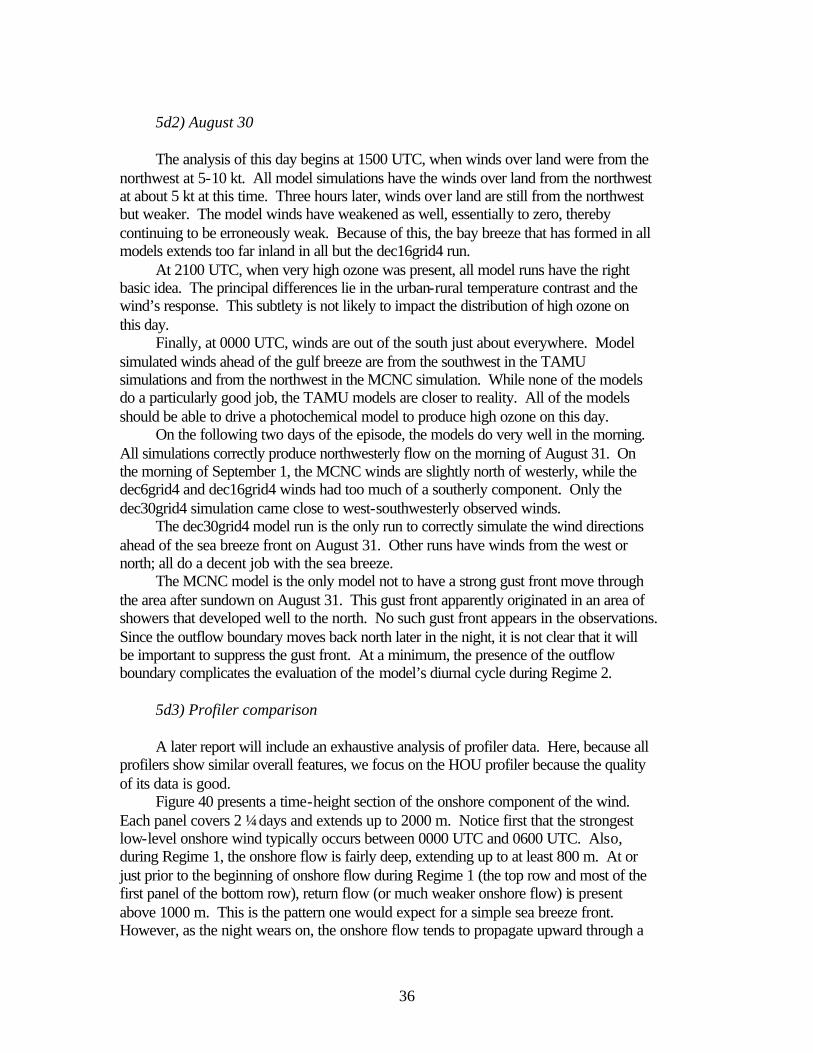
36

5d2) August 30 The analysis of this day begins at 1500 UTC, when winds over land were from the northwest at 5-10 kt. All model simulations have the winds over land from the northwest at about 5 kt at this time. Three hours later, winds over land are still from the northwest but weaker. The model winds have weakened as well, essentially to zero, thereby continuing to be erroneously weak. Because of this, the bay breeze that has formed in all models extends too far inland in all but the dec16grid4 run. At 2100 UTC, when very high ozone was present, all model runs have the right basic idea. The principal differences lie in the urban-rural temperature contrast and the wind’s response. This subtlety is not likely to impact the distribution of high ozone on this day. Finally, at 0000 UTC, winds are out of the south just about everywhere. Model simulated winds ahead of the gulf breeze are from the southwest in the TAMU simulations and from the northwest in the MCNC simulation. While none of the models do a particularly good job, the TAMU models are closer to reality. All of the models should be able to drive a photochemical model to produce high ozone on this day. On the following two days of the episode, the models do very well in the morning. All simulations correctly produce northwesterly flow on the morning of August 31. On the morning of September 1, the MCNC winds are slightly north of westerly, while the dec6grid4 and dec16grid4 winds had too much of a southerly component. Only the dec30grid4 simulation came close to west-southwesterly observed winds. The dec30grid4 model run is the only run to correctly simulate the wind directions ahead of the sea breeze front on August 31. Other runs have winds from the west or north; all do a decent job with the sea breeze. The MCNC model is the only model not to have a strong gust front move through the area after sundown on August 31. This gust front apparently originated in an area of showers that developed well to the north. No such gust front appears in the observations. Since the outflow boundary moves back north later in the night, it is not clear that it will be important to suppress the gust front. At a minimum, the presence of the outflow boundary complicates the evaluation of the model’s diurnal cycle during Regime 2. 5d3) Profiler comparison A later report will include an exhaustive analysis of profiler data. Here, because all profilers show similar overall features, we focus on the HOU profiler because the quality of its data is good. Figure 40 presents a time-height section of the onshore component of the wind. Each panel covers 2 ¼ days and extends up to 2000 m. Notice first that the strongest low-level onshore wind typically occurs between 0000 UTC and 0600 UTC. Also, during Regime 1, the onshore flow is fairly deep, extending up to at least 800 m. At or just prior to the beginning of onshore flow during Regime 1 (the top row and most of the first panel of the bottom row), return flow (or much weaker onshore flow) is present above 1000 m. This is the pattern one would expect for a simple sea breeze front. However, as the night wears on, the onshore flow tends to propagate upward through a

37

fairly deep layer, and strong onshore flow is found around 1200 UTC at 2000 m on most days. Figure 41 shows the time-height section for the same location from dec6grid4. The other TAMU runs are broadly similar. During Regime 1, the simulated onshore flow seems to be too shallow, with the core of strongest winds centered around 200 m rather than 600 m. Also, the winds die away too rapidly. Aloft, the return flow is well simulated. The model also shows some evidence of downward phase propagation, which is consistent with theories of the subtropical sea breeze. During Regime 2, observations show a stronger oscillation, one that is less deep in extent. The model shows the same qualitative differences between Regime 1 and Regime 2, but the model is also too shallow with its wind variations. The MCNC output is shown in Fig. 42. The same regular cycle as in the observations and dec6grid4 output shows up here too, but the amplitude is weaker, consistent with the MCNC model’s underestimate of the diurnal temperature cycle, which forces this circulation. And while the onshore flow decreased too rapidly in the dec6grid4 model run, it decreases even more rapidly in the MCNC run. During Regime 2, discontinuities in the plotted data are easy to spot every twelve hours, implying that during this weather regime the model is generating a considerably different wind pattern than is in the EDAS analyses. The alongshore component of the wind tells a more interesting story. The diurnal heating does not produce a pressure gradient in the alonshore direction. Instead, the alongshore component of wind arises from turning of the onshore component of wind by the Coriolis force. The observed alongshore wind (Fig. 43) shows a much cleaner vertical phase propagation during Regime 1 than the onshore wind. As expected, the alongshore component reaches its maxima and minima about six hours after the onshore component. This alongshore flow occurs later at higher altitudes, but the magnitude of the alongshore perturbation is barely diminished. During Regime 2, the wind perturbations do not extend upward as far and low-level jets develop at night with wind speeds of over 14 m/s. The dec6grid4 simulation (Fig. 44) has the right qualitative structure in Regime 1, but the upward phase propagation does not seem to be as strong. During Regime 2, the low-level jets that the model produces are two weak, too shallow, and evolve differently. The MCNC alongshore wind (Fig. 45) has less coherent phase propagation than the observations or the other model. The MCNC model seems seriously deficient during Regime 2, as on three consecutive nights a nighttime low-level jet does not form in the 5 km simulation but appears magically at 1200 UTC as the next model cycle kicks in. On the whole, the MCNC model seems less able to model the wavelike properties of the diurnal wind cycle than the TAMU models.

38

6. Conclusion 6a: TAMU Models In this report, three of the more successful TAMU simulations were compared to observations, in order to assess how well the simulations reproduced important weather features. The dec6grid4 and dec30grid4 model runs were found to be quite similar and quite successful, and the final MM5 simulations will be based upon them. The two runs accurately predicted maximum temperatures and their horizontal distribution, precipitation events, and horizontal wind distributions. The model simulations were less successful at simulating minimum temperatures and nocturnal temperature inversions, the vertical variation of wind, the nighttime urban heat island, and the daytime urban heat island (or lack thereof). The third model, dec16grid4, is superior in performance in such aspects as the diurnal wind cycle, but the overforecasting of clouds and precipitation make use of the model as a photochemical driver difficult. None of the models produced daytime clouds that resembled the actual clouds during TexAQS-2000. Of the remaining deficiencies in the model, it will probably not be possible to correct the nighttime temperature bias. The nighttime and daytime heat islands may be correctable through judicious specification of land surface characteristics. All three deficiencies may have a minor but not inconsequential impact on ozone evolution. A fourth deficiency, the model’s handling of the vertical variation of the diurnal wind cycle, will be analyzed more fully in the next weeks. Some improvement is virtually guaranteed when data assimilation is implemented, but it is hoped that physical changes to the model can improve the model’s dynamics somewhat beforehand. 6b: MCNC Model The MCNC model was inferior to the TAMU models because of the poor diurnal temperature cycle, a consequence of erroneously high moisture availability. This led to weak diurnal wind cycles and likely poor pollutant transport in coastal areas. Clouds tended to be too widespread and rainfall was poorly forecasted. On balance, we conclude that the current best TAMU MM5 simulations beat the real-time forecast configuration of the MCNC model.

39

Figure 1: Horizontal extent of the TAMU 4 km domain (dark shading) and MCNC 5 km domain (embedded light shading).

40

Figure 2: Locations of wind profiler sites and doppler lidar (LAP). Background is land use category from the TAMU 4 km grid.

41

La Porte Lidar Low-Level Jet

0

0.5

1

1.5

2

2.5

3

3.5

4

0 2 4 6 8 10 12 14 16

Wind speed (m/s)

Hei

gh

t rel

ativ

e to

leve

l of m

axim

um

win

ds

12 UTC Sept 1

12 UTC Aug 31

Figure 3: Vertical structure of low-level jet, 1200 UTC August 31 (blue) and 1200 UTC September 1 (pink), from doppler lidar data. Because of a malfunction of the lidar, the height of the data points is only known relative to the height of the wind maximum. The dashed black line is a linear extrapolation of the wind profile to the surface.

42

Figure 4: Daily accumulated precipitation (cm), August 23-September 1, as simulated by the dec30grid4 model run. Note that two days are combined in the lower left panel.

43

Figure 5: Daily accumulated precipitation (cm), August 23-September 1, as simulated by the dec30grid4 model run. Note that two days are combined in the lower left panel.

44

Figure 6: Daily accumulated precipitation (cm), August 23-September 1, as simulated by the dec16grid4 model run. Note that two days are combined in the lower left panel.

45

Figure 7: Daily accumulated precipitation (cm), August 23-September 1, as simulated by the MCNC model run. Note that two days are combined in the lower left panel.

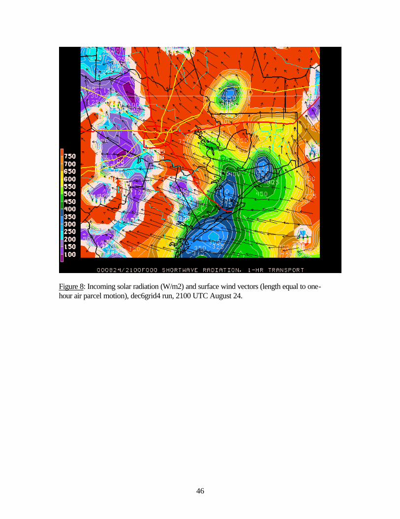
46

Figure 8: Incoming solar radiation (W/m2) and surface wind vectors (length equal to one-hour air parcel motion), dec6grid4 run, 2100 UTC August 24.

47

Figure 9: Low-level reflectivity scan, Houston/Galveston WSR-88D doppler radar, 2102 UTC August 24, showing heavy rain (reds), light to moderate rain (greens and yellows), and outflow boundary (arc-shaped dark blue lines north and west of Houston).

48

Figure 10: Incoming solar radiation (W/m2) and surface wind vectors (length equal to one-hour air parcel motion), dec30grid4 run, 2100 UTC August 24.

49

Figure 11: Incoming solar radiation (W/m2) and lowest sigma level wind vectors (length equal to one-hour air parcel motion), MCNC run, 1500 UTC August 28.

50

Figure 12: Incoming solar radiation (W/m2) and lowest sigma level wind vectors (length equal to one-hour air parcel motion), dec16grid4 run, 1500 UTC August 28.

51

Figure 13: Incoming solar radiation (W/m2) and surface wind vectors (length equal to one-hour air parcel motion), dec30grid4 run, 1500 UTC August 28.

52

Figure 14: Visible satellite image, 1515 UTC 28 August.

53

Houston Area NWS Stations

20

25

30

35

40

Aug 23 - Sept 1, 2000

Te

mp

era

ture

(C

)

dec6grid4Observations

dec30grid4

Figure 15: Maximum and minimum temperatures (C) during the August 2000 ozone episode at eight National Weather Service surface stations in the Houston/Galveston area, compared to 2 m temperatures simulated by the dec6grid4 and dec30grid4 model runs.

54

Comparison of 2m and 17m Maximum/Minimum Temperatures

20

25

30

35

40

Aug 23 - Sept 1, 2000

Te

mp

era

ture

(C

)

dec30 2m

dec30 19m

Figure 16: Comparison of daily maximum and minimum temperatures at seven surface observing sites in the Houston-Galveston area, as simulated at 2 m and 17 m height above ground level by the dec30grid4 model run.

55

17-19 m Maximum/Mininum Temperatures

20

25

30

35

40

Aug 23 - Sept 1, 2000

Te

mp

era

ture

(C

)

dec30grid4dec16grid4s

mcnc

Figure 17: Maximum and minimum temperatures at the 17 m level (TAMU runs) and 19 m level (MCNC run) at seven National Weather Service observing sites in the Houston/Galveston area during the ozone episode.

56

Figure 18: Surface observations, 1500 UTC August 31. Temperatures (F) are blue, dewpoints (F) are green, ozone (ppbv) is white, winds (long barb = 10 kt) are yellow.

57

Figure 19: Surface (2 m) temperatures (F) and (10 m) winds, dec30grid4 model run, 1500 UTC August 31.

58

Figure 20: Lowest sigma layer temperatures (F) and winds, dec16grid4 model run, 1500 UTC August 31.

59

Figure 21: Surface (2 m) temperatures (F) and (10 m) winds, dec6grid4 model run, 1500 UTC August 31.

60

Figure 22: Lowest sigma layer temperatures (F) and winds, MCNC model run, 1500 UTC August 31.

61

Figure 23: Surface observations, 2100 UTC August 31.

62

Figure 24: Surface (2 m) temperatures (F) and (10 m) winds, dec30grid4 model run, 2100 UTC August 31.

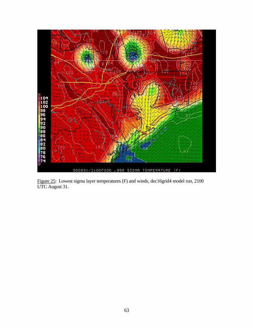
63

Figure 25: Lowest sigma layer temperatures (F) and winds, dec16grid4 model run, 2100 UTC August 31.

64

Figure 26: Surface (2 m) temperatures (F) and (10 m) winds, dec6grid4 model run, 2100 UTC August 31.

65

Figure 27: Lowest sigma layer temperatures (F) and winds, MCNC model run, 2100 UTC August 31.

66

Figure 28: Surface (2 m) temperatures (F) and (10 m) winds, dec6grid4 model run, 1500 UTC August 28.

67

Figure 29: Surface observations, 1500 UTC August 28.

68

Figure 30: Lowest sigma level temperatures (F) and winds, dec16grid4 model run, 1500 UTC August 28.

69

Figure 31: Surface weather observations, 2100 UTC August 28.

70

Figure 32: Surface (2 m) temperatures (F) and (10 m) winds, dec30grid4 model run, 2100 UTC August 28.

71

Figure 33: Vertical soundings of temperature (right, C) and dewpoint (left, C), 1100 UTC August 31, Wharton Power Plant (WPP). Maroon: observed. Orange: dec6grid4. Blue: dec30grid4. Green: dec16grid4. Magenta: MCNC. Observed wind vectors are plotted to the right.

72

Figure 34: Vertical soundings of temperature and dewpoint, as in Fig. 33, but for 1100 UTC August 27.

73

Figure 35: Vertical soundings of temperature and dewpoint, as in Fig. 33, but for 2000 UTC August 31.

74

Figure 36: Surface weather observations, 1800 UTC August 25

75

Figure 37: Surface (2 m) temperatures (F) and (10 m) winds, dec6grid4 model run, 1800 UTC August 25.

76

Figure 38: Lowest sigma level winds and temperatures, dec16grid4 model run, 1800 UTC August 25.

77

Figure 39: Lowest sigma level winds and temperatures, MCNC model run, 1800 UTC August 25.

78

Figure 40: Time-height cross section of observed onshore component of wind (toward 330 degrees) at HOU profiler site. Wind is contoured every 1 m/s with negative (toward sea) values dashed. The four panels, reading from left to right, begin at 1200 UTC August 24, 26, 28, and 30 and extend for 2 days and 6 hours, so that there is some overlap. The y axis is height above ground level, with grid lines every 200 m.

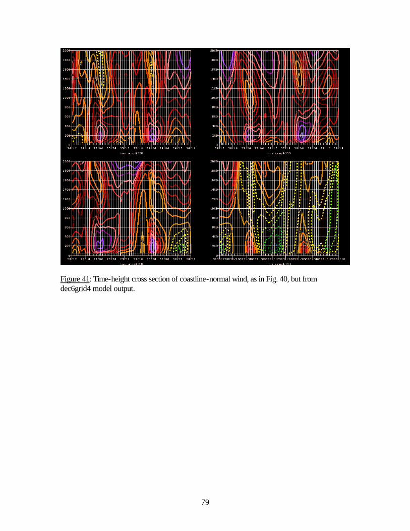
79

Figure 41: Time-height cross section of coastline-normal wind, as in Fig. 40, but from dec6grid4 model output.

80

Figure 42: Coastline-normal wind, as in Figs. 40 and 41, but from MCNC model output.

81

Figure 43: Coastline-parallel wind, positive toward the northeast (30 degrees), from HOU consensus profiler observations. Plotting conventions as in Fig. 40.

82

Figure 44: Coastline parallel winds, as in Fig. 43, but from dec6grid4 model output.

83

Figure 45: Coastline-parallel winds, as in Fig. 43, but from MCNC model output.