Evaluation and Visualization of Stress and Strain on Soft Biological Tissues in Contact

Sofiane Sarni, Anderson Maciel, Ronan Boulic, Daniel ThalmannVirtual Reality Lab (VRlab), Swiss Federal Institute of Technology (EPFL)

CH-1015 Lausanne, Switzerland.sofiane.sarni@epfl.ch, anderson.maciel@epfl.ch, ronan.boulic@epfl.ch, daniel.thalmann@epfl.ch

Abstract

This paper addresses evaluation and visualization ofstress and strain on soft biological tissues in contact.Given three-dimensional models of reconstructed organsfrom magnetic resonance images (MRI), we use anAnatomy-based kinematical model combined with a softtissues model to represent their shape and behavior.Then, we compute resulting distribution of stress andstrain on deforming surface when motion is simulated.The computed stress and strain are then effectivelyvisualized using an interactive animation framework.Experimental results are illustrated in the case of the hipjoint cartilage.

1. Introduction

Evaluation of stress and strain is a typical analysismethod of three-dimensional bodies. It allows estimatingthe deformation of an object under given load conditions.That is why it is being widely used in CAD/CAMapplications and also in medical applications, especiallythose related to biomechanics where it is important toassess joints congruity [6]. For instance, assessing stressand strain allows analyzing joint surface, which helps indiagnosing possible pathologies or planning surgery.

Approaches for modeling object deformation rangefrom non-physical methods to methods based oncontinuum mechanics which account for the effects ofmaterial properties, external forces, and environmentalconstraints or object deformation [9]. Here we focus onspecific physically based approaches, which are used formodeling soft tissues and compute related physicalquantities. In this category, we find mass-spring systemsand finite element methods. Other physically basedmethods used to model deformable objects includeimplicit surfaces and particles systems but are notconsidered here.

Our approach to model soft tissues relies on ageneralized mass-spring model where mass points are, infact, spherical mass regions called molecules. Elasticforces are established between molecules by spring-like

connections. This model integrates properties of realbiological materials to define the stiffness of thoseconnections.

We compute the distribution of stress and strain ondeforming surface when motion is simulated. The stressand strain calculated by means of the deformation modelare color mapped on the meshes representing organs toindicate variation during motion. Experimental results areillustrated in the case of hip joint cartilage.

2. Related Work

2.1. Mass-spring systems

The mass-spring method is a physically basedtechnique that has been used widely and effectively formodeling deformable objects. An object is modeled as acollection of point masses connected by springs in alattice structure. Springs connecting point masses exertforces on neighboring points when a mass is displacedfrom its rest position (Figure 1).

Mass-spring systems have been widely used in facialanimation. Terzopoulos and Waters used a three-layersmesh of mass points associated to three anatomicallydistinct layers of facial tissue (dermis, subcutaneous fattytissue, and muscle) [23]. To improve realism, Lee et al.added further constraints to prevent penetrations betweensoft tissues and bone [13]. In [20], mass-spring systemswere used to simulate muscle deformation. Muscles wererepresented at two levels: action lines and muscle shape.This shape was deformed using a mass-spring mesh. Inorder to control the volume of muscles during deformation and smooth out mesh discontinuities, “angular springs”were introduced. These springs differ from other springsby the way they are attached. In this work, emphasis wasput on interaction rather than simulation quality. Aubelused a similar approach with a multi-layered model basedon physiological and anatomical considerations [1].Bourguignon and Cani proposed a model offering controlof the isotropy or anisotropy of elastic material [3]. Mass-spring models do not have this property. The basic idea of their approach is to let the user define, everywhere in theobject, mechanical characteristics of the material along a

given number of axes corresponding to orientation ofinterest. All internal forces will be acting along these axes instead of acting along the mesh edges. Mass springsystems have also been used for cloth motion [2] andsurgical simulation [21][5]. In a more recent work,Jansson et al. used a discrete mechanical model that canbe viewed as a generalized mass-spring model forapplications in computer-aided design [11].

Figure 1. Portion of a mass-spring model.(Reprinted from [9])

Mass-spring models are easy to construct, and bothinteractive and real-time simulations of mass-springsystems are possible even with desktop systems. Anotherwell-known advantage is their ability to handle both largedisplacements and large deformations. Mass-springsystems have some drawbacks. Since the model is tunedthrough its spring constants, good values for theseconstants are not always easy to derive from measuredmaterial properties. Furthermore, it is difficult to expresscertain constraints (like incompressibility and anisotropy)in a natural way. Another problem occurs when springconstants are large. Such large constants are used tomodel nearly rigid objects, or model non-penetrationbetween deformable objects. This problem is referred asstifness. Stiff systems are problematic because of theirpoor stability, which requires small time steps fornumerical integration resulting in slow simulation [9].

2.2. Finite Element

Whereas mass-spring models start with a discreteobject model, more accurate physical models considerdeformable objects as a continuum: solid body with massand energies distributed throughout. Models can bediscrete or continuous but the method used for solving isdiscrete. Finite element method is used to find anapproximation for a continuous function that satisfies

some equilibrium expression. In FEM, the continuum(object) is divided into elements joined at discrete nodepoints. A function that solves the equilibrium equation isfound for each element.

FEM has been widely used in soft tissues modeling.Debunne et al. used a space and time adaptive level ofdetail, in combination with a large displacement straintensor formulation [7]. To solve the system, explicit FEMwas used where each element is solved independentlythrough a local approximation, which reducescomputational time. Hirota et al. used FEM in simulationof mechanical contact between nonlinearly elastic objects[10]. The mechanical system used as a case study was thehuman leg, more precisely, the Visible Human right kneejoint and some of its surrounding bones, muscles, tendons and skin. The approach relied on a novel penalty finiteelement formulation based on the concept of materialdepth to compute skin, tendons and muscles deformation.By linearly interpolating pre-computed material depths atnode points of the finite element mesh, contact forces canbe analytically integrated over contacting regions withoutraising computational cost. The algorithm wasimplemented as a part of an implicit finite elementprogram for dynamic, quasi-static and static analysis ofnonlinear viscoelastic solids. High nonlinearity andanisotropy typically observed for biological materialswere also supported. To achieve real-time deformation,reducing computing time is necessary. Bro-Nielsen andCotin studied this problem by using a condensationtechnique [4]. With this method, the computation timerequired for the deformation of a volumetric model can be reduced to the computation time of a model onlyinvolving the surface nodes of the mesh.

Finite element methods provide a more realisticsimulation than mass-spring methods but are lesscomputationally efficient. In addition, the linear elastictheory used to derive the potential energy equationassumes small deformation of the object, which is true for materials such as metal. However, for soft biologicalmaterial, objects dimensions can deform in largeproportions so that the small deformation assumption nolonger holds. Because of this change, the amount ofcomputation required at each time is greatly increased.

3. Deformable Model

Our approach to model soft tissues is inspired from the work of Jansson et al. [11]. Their work exploits ageneralized mass-spring model – which they callmolecular model – where mass points are, in fact,spherical mass regions called molecules. Elastic forces are then established between molecules by a spring-likeconnection.

Our contribution to this model is in the integration ofproperties of real biological materials to define thestiffness of its spring-like connections. We tested severalapproaches and selected the one that we can generalize for arbitrary distributions of masses and springs. Therheological standard to define the elasticity of a material is Young’s modulus. Young’s modulus is a property of amaterial, not of an object. So, it is independent of theobject’s shape. However, when one discretizes an objectby a set of springs, the stiffness k of every spring must beproportional to the fraction of the volume of the object itrepresents. It means that if a cube of side l0 is compressed by a force F, it should shorten in the direction of the force, of the same elongation variation ∆l both if it isrepresented by only one spring and if it is discretized by n springs. Equation 3 establishes the Young’s modulus Efrom the knowledge of the elongation variation ∆l, anapplied force F, the length of the object in rest conditions l0, and the cross-sectional area of the object A. ApplyingEq.3 iteratively in the simulation loop we can minimizethe difference between the obtained and the aimed Eincreasing or reducing the value of k’s accordingly. Seemore details in [18].

The Force Model. The model is described by two sets of elements: E, a set of spherical massive elements(molecules), and C, a set of connections between theelements in E (Eq. 1).

{ }neeeE L,, 21= ; { }neee CCCC L,,

21= ;

{ }me cccCi

L,, 21=

(1)

The model’s behavior is determined by the forcesproduced on each element of E by each connection of Cand some external forces.

collisionsCLGe FFFFFrrrrr

+++= (2)

where

gmF eG

rr=

(3)

e

eeeL

V

VVrF r

rrr 22 ρΠ−=

(4)

fdbC FFFFrrrr

++= (5)

FG: gravity (me is the mass of e and g is the gravityacceleration);FL: ambient viscous friction (r is the radius, ? is themedium density and V is the velocity);FC: connection forces, see Eq. 6.

fdbC FFFFrrrr

++= (6)

where

( )pe

peC

icpecb

PP

PPlPPkF

e

rr

rrrrr

−

−−−−= ∑

=0 (7)

( )VbFeC

icd

rr

∑=

−=0 (8)

( ) ( )( )pe

pe

pepe PPPP

PPVVV

rr

rr

rrrrr

−−

−⋅−=

2

(9)

⊥⊥−= ∑

= V

VFF

eC

i

Nef r

rrr

0

µ (10)

dbN FFFrrr

+= (11)

( ) VVVV pe

rrrr−−=⊥ (12)

Fb: elasticity (kc is the spring Hooke’s constant, lc is thespring elongation, and Pe and Pp are the positions of theelements involved with connection c);Fd: internal damping (bc is the damping coefficient, P and V are respectively the positions and velocities of theelements involved with connection c);Ff: sliding friction (µe is the friction constant for the element and FN is the force normal to friction direction).

Al

lFE

⋅∆⋅

= 0 (3)

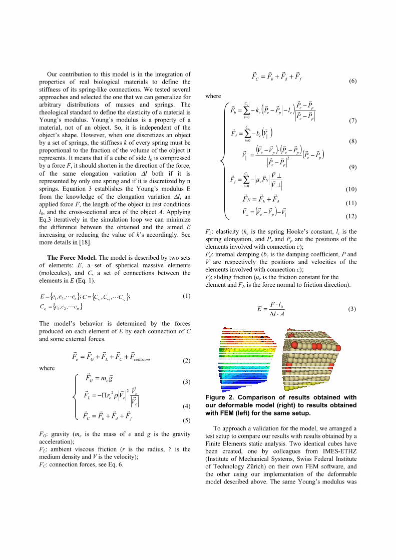
Figure 2. Comparison of results obtained withour deformable model (right) to results obtainedwith FEM (left) for the same setup.

To approach a validation for the model, we arranged a test setup to compare our results with results obtained by a Finite Elements static analysis. Two identical cubes havebeen created, one by colleagues from IMES-ETHZ(Institute of Mechanical Systems, Swiss Federal Instituteof Technology Zürich) on their own FEM software, andthe other using our implementation of the deformablemodel described above. The same Young’s modulus was

used on the two objects, the same constant forces wereapplied onto them, and the results were compared. Visualresults for a shear force applied on the upper face areshown in Figure 2. Besides the visual results that looksimilar, we also compared the displacement of key pointstracked on both objects. These points represented onfigure 2 by red spheres underwent the samedisplacements.

4. Anatomy-Based Kinematical Model

A kinematical model represents the human bodyarticulated system as a tree where joints correspond to the nodes of the tree. Organs like bones and cartilage caps are instantiated into this node to give anatomical appearanceto a human body part, (Figures 3). Any generic joint isable to describe any kind of relative motion between twoor more adjacent segments of the body. Such motion canbe given by: a) a rotation around one axis; b) a composed rotation around two or three axis; c) a translation in one to three Cartesian directions; d) rotations associated totranslations; and e) an axis sliding on a parametric curveduring rotation.

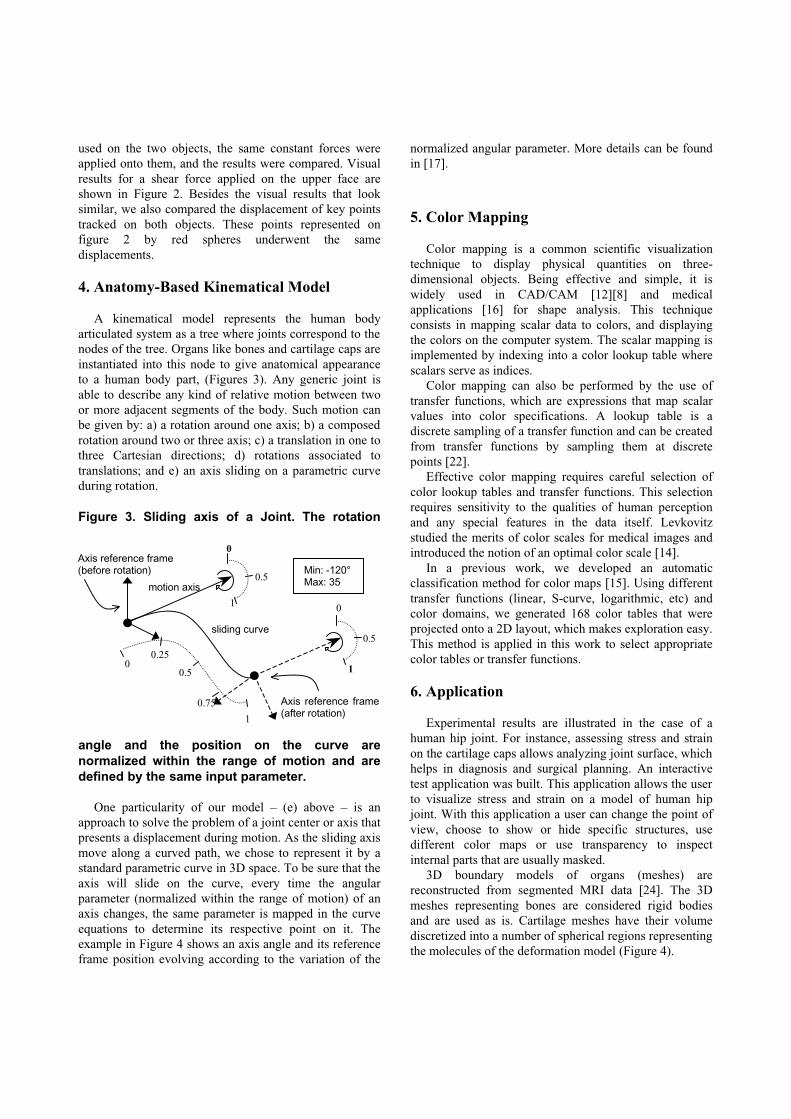
Figure 3. Sliding axis of a Joint. The rotation

angle and the position on the curve arenormalized within the range of motion and aredefined by the same input parameter.

One particularity of our model – (e) above – is anapproach to solve the problem of a joint center or axis that presents a displacement during motion. As the sliding axis move along a curved path, we chose to represent it by astandard parametric curve in 3D space. To be sure that the axis will slide on the curve, every time the angularparameter (normalized within the range of motion) of anaxis changes, the same parameter is mapped in the curveequations to determine its respective point on it. Theexample in Figure 4 shows an axis angle and its referenceframe position evolving according to the variation of the

normalized angular parameter. More details can be foundin [17].

5. Color Mapping

Color mapping is a common scientific visualizationtechnique to display physical quantities on three-dimensional objects. Being effective and simple, it iswidely used in CAD/CAM [12][8] and medicalapplications [16] for shape analysis. This techniqueconsists in mapping scalar data to colors, and displayingthe colors on the computer system. The scalar mapping isimplemented by indexing into a color lookup table wherescalars serve as indices.

Color mapping can also be performed by the use oftransfer functions, which are expressions that map scalarvalues into color specifications. A lookup table is adiscrete sampling of a transfer function and can be created from transfer functions by sampling them at discretepoints [22].

Effective color mapping requires careful selection ofcolor lookup tables and transfer functions. This selectionrequires sensitivity to the qualities of human perceptionand any special features in the data itself. Levkovitzstudied the merits of color scales for medical images andintroduced the notion of an optimal color scale [14].

In a previous work, we developed an automaticclassification method for color maps [15]. Using differenttransfer functions (linear, S-curve, logarithmic, etc) andcolor domains, we generated 168 color tables that wereprojected onto a 2D layout, which makes exploration easy. This method is applied in this work to select appropriatecolor tables or transfer functions.

6. Application

Experimental results are illustrated in the case of ahuman hip joint. For instance, assessing stress and strainon the cartilage caps allows analyzing joint surface, which helps in diagnosis and surgical planning. An interactivetest application was built. This application allows the user to visualize stress and strain on a model of human hipjoint. With this application a user can change the point ofview, choose to show or hide specific structures, usedifferent color maps or use transparency to inspectinternal parts that are usually masked.

3D boundary models of organs (meshes) arereconstructed from segmented MRI data [24]. The 3Dmeshes representing bones are considered rigid bodiesand are used as is. Cartilage meshes have their volumediscretized into a number of spherical regions representing the molecules of the deformation model (Figure 4).

0

1

0.5motion axis

Min: -120°Max: 35

1

0

0.5

00.25

1

0.5

0.75

sliding curve

Axis reference frame(after rotation)

Axis reference frame (before rotation)

Figure 4. The cartilage cap of the acetabular cupdiscretized into a set of spherical regions.

The vertices on the surfaces of the cartilage caps arethen linked to the neighborhood of underlying moleculeswith weights according to distances, and follow the model deformations. Surface molecules are used to generatecontact avoidance forces. These forces, that are calculated using a penalty method [19], are consequently used by the deformation model to produce deformation. Motion isgenerated using the kinematical model (Figure 5). Finally, stress is calculated relating these forces with their area ofactuation, and strain is calculated relating the original and current distances between molecules centers.

Figure 5. Kinematical hip. In this model the usual rotational axes are not constrained to rotatearound a fixed point. The center of rotation canslide according to the angular position of thejoint.

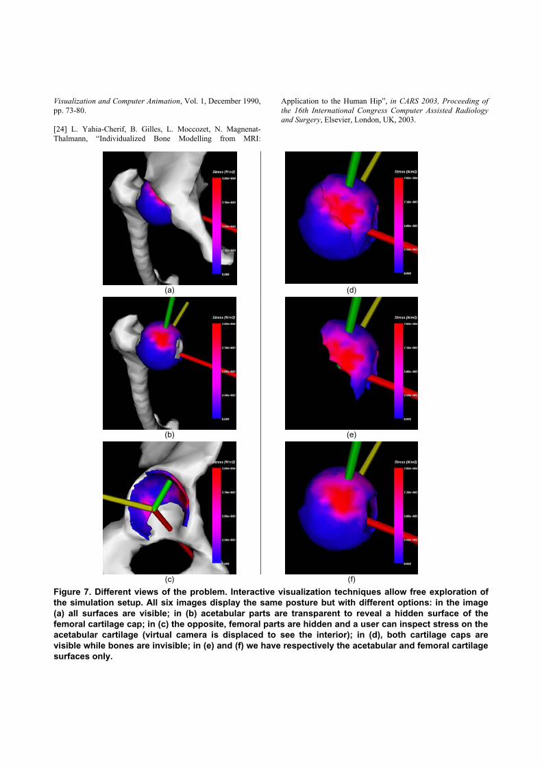
The last step is using color mapping for effectivevisualization of these values (Figures 6). Interactivevisualization techniques allow free exploration of thesimulation setup (Figure 7). All six images display thesame posture but with different options: in the image (a)all surfaces are visible; in (b) acetabular parts aretransparent to reveal a hidden surface of the femoralcartilage cap; in (c) the opposite, femoral parts are hidden and a user can inspect stress on the acetabular cartilage(virtual camera is displaced to see the interior); in (d),both cartilage caps are visible while bones are invisible; in (e) and (f) we have respectively the acetabular and

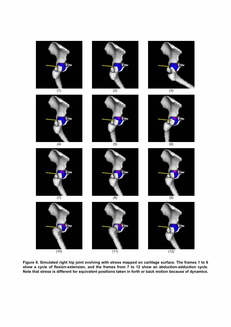
femoral cartilage surfaces only. A simulation of evolvingstress during motion is also presented on Figure 8.

Figure 6. Stress distribution mapping on hip joint cartilage using a S-curve, blue-to-red transferfunction.

7. Summary

In this paper, we have presented the combination of adeformable model for biological soft tissues with ananatomy-based kinematical model of human joints, whichwe used to simulate motion on the hip joint and evaluatestress and strain on cartilage surfaces.

The model demonstrated its ability to handle the stress-strain computation for two coupled surfaces withinteractive user control. Associated to our palette ofvisualization tools, the user interaction can easilyhighlight regions subject to high stress, hence topathologies.

At this moment, the deformation model is linear elastic and isotropic. We are working to improve it by addingviscous components and considering fibers orientation inthe tissue. We aim at making it a viscoelastic, anisotropicand heterogeneous model, which is closer to the nature ofthe real biological tissues. It is crucial to support theenvisaged medical applications. Future work also includesthe evaluation of joint range of motion using theinformation given by stress distribution.

8. Acknowledgement

This work was supported by the Swiss NationalScience Foundation (SNF) in the framework of theNational Center of Competence in Research for Computer Aided and Image Guided Medical Interventions(NCCR/CO-ME). We thank Lydia Yahia-Cherif from theMIRALab at University of Geneva for providing the 3-Dmodels and Dr. Hassan Sadri, MD, from the Orthopedics

Department of the Fribourg Hospital for his support withthe simulation of the hip joint.

References

[1] A. Aubel, and D. Thalmann, “Interactive Modeling ofHuman Musculature”, Computer Animation 2001, Seoul, Korea, November 7-8, 2001.

[2] D. Baraff, and A. Witkin, “Large Steps in Cloth Simulation”,Proceedings of ACM SIGGRAPH’98, ACM SIGGRAPH, 1998, pp. 43-54.

[3] D. Bourguignon, and M.-P. Cani, “Controlling Anisotropy in Mass-Spring Systems”, Computer Animation and Simulation2000, Interlaken (Switzerland), August 21-22, 2000, pp. 113-123.

[4] M. Bro-Nielsen, and S. Cotin, “Real-time VolumetricDeformable Models for Surgery Simulation using FiniteElements and Condensation”, Computer Graphics Forum(Eurographics'96), 15(3), 1996, pp. 57-66.

[5] J. Brown, S. Sorkin, C. Bruyns, J.-C. Latombe, K.Montgomery, and M. Stephanides, “Real-Time Simulation ofDeformable Objects: Tools and Application”, In ComputerAnimation 2001, Seoul, Korea, November 7-8, 2001.

[6] B. Z. A. Cohen, D. M. McCarthy, S. D. Kwark, P. Legrand,F. Fogarasi, E. J. Ciaccio, and G. A. Ateshian. “Knee CartilageTopography, Thickness, and Contact Areas from MRI: in-vitroCalibration and in-vivo Measurements”, Osteoerthritis andCartilage, 7, OsteoArthritis Research Society International,1999, pp. 95-109.

[7] G. Debunne, M. Desbrun, M.-P. Cani, and A. H. Barr,“Dynamic Real-Time Deformations Using Space and TimeAdaptive Sampling”, Proceedings of SIGGRAPH 2001,Computer Graphics Proceedings, ACM SIGGRPAH, August2001, pp. 31-36.

[8] R. S. Gallagher and J. C. Nagtegaal, “An Efficient 3-DVisualization Technique for Finite Element Models and OtherCoarse Volumes”, Proceedings of SIGGRAPH '89, ACMSIGGRAPH, Boston, USA, July 31-August 4, 1989, pp. 185-193.

[9] S. F. Gibson, and B. Mirtich, “A Survey of DeformableModeling in Computer Graphics”, Technical Report No. TR-97-19, Mitsubishi Electric Research Lab., Cambridge, USA,November 1997.

[10] G. Hirota, S. Fisher, C. Lee, A. State, and H. Fuchs, “AnImplicit Finite Element Method for Elastic Solids in Contact”,Computer Animation 2001, Seoul (Korea), 2001.

[11] J. Jansson, and J. S. M Vergeest, “A Discrete MechanicsModel for Deformable Bodies”, Computer-Aided Design, Vol.34 (12), Elsevier Science, Amsterdam, 2002, pp. 913-928.

[12] S. Kuschfeldt, T. Ertl, and M. Holzner, “EfficientVisualization of Physical and Structural Properties in Crash-Worthiness Simulations (Case Study)”, In Proceedings of IEEEVisualization '97, IEEE Computer Society and ACM, Phoenix,USA, October 19-24, 1997, pp. 487-490.

[13] Y. Lee, and D. Terzopoulos and K. Waters, “RealisticModeling for Facial Animation”, Proceedings of SIGGRAPH 95, Computer Graphics Proceedings, Annual Conference Series,Los Angeles, USA, August 1995, pp. 55-62.

[14] H. Levkowitz, and G. T. Herman, “Color Scales for ImageData”, IEEE Computer Graphics & Applications, 12 (1), IEEEComputer Society, USA, 1992, pp. 72-80.

[15] I. S. Lim, P. H. Ciechomski, S. Sarni, and D. Thalmann“Planar Arrangement of High-dimensional Biomedical Data Sets by Isomap Coordinates”, Proceedings of the 16th IEEESymposium on Computer-Based Medical Systems (CBMS 2003),IEEE Computer Society, New York, USA, June 26-27, 2003, pp. 50-55.

[16] I. S. Lim, S. Sarni, and D. Thalmann, “ColoredVisualization of Shape Differences between Bones”,Proceedings of the 16th IEEE Symposium on Computer-BasedMedical Systems (CBMS 2003), IEEE Computer Society, NewYork, USA, June 26-27, 2003, pp. 273-278.

[17] A. Maciel, L.P. Nedel and C.M.D.S. Freitas, “Anatomy-Based Joint Models for Virtual Human Skeletons”, Proceedingsof the Computer Animation 2002 Conference, Geneva, IEEEComputer Society, pp. 220-224, 2002.

[18] A. Maciel, R. Boulic, and D. Thalmann, “DeformableTissue Parameterized by Properties of Real Biological Tissue”In. International Symposium on Surgery Simulation and SoftTissue Modeling, 2003, Editors Nicholas Ayache & HerveDelingette, Springer-Verlag, Juan-les-Pins, France, 2003, pp.76-89.

[19] J.C. Platt and A. H. Barr. “Constraint Methods for FlexibleModels”, In Computer Graphics (Proc. SIGGRAPH), Vol. 22,No. 4, ACM SIGGRAPH, August 1988, pp. 279-288.

[20] L. Porcher-Nedel, and D. Thalmann. “Real Time MuscleDeformations Using Mass-Spring Systems”, Computer Graphics International 1998, Hannover (Germany), June 1998, pp. 156-165.

[21] A. Radetzky, A Nürnberger, M. Teistler, D.P. Pretschner,“Elastodynamic shape modeling in virtual medicine”,International Conference on Shape Modeling and Applications,IEEE Computer Society Press, Piscataway, NJ, 1999, pp. 172-178.

[22] W. Schroeder, K. Martin, and B. Lorensen, TheVisualization Toolkit: An Object-Oriented Approach to 3-DGraphics (2nd Edition), Prentice Hall, New Jersey, USA, 1997.

[23] D. Terzopoulos, and K. Waters, “Physically-Based FacialModeling, Analysis, and Animation”, The Journal of

Visualization and Computer Animation, Vol. 1, December 1990, pp. 73-80.

[24] L. Yahia-Cherif, B. Gilles, L. Moccozet, N. Magnenat-Thalmann, “Individualized Bone Modelling from MRI:

Application to the Human Hip”, in CARS 2003, Proceeding ofthe 16th International Congress Computer Assisted Radiologyand Surgery, Elsevier, London, UK, 2003.

(a) (d)

(b) (e)

(c) (f)

Figure 7. Different views of the problem. Interactive visualization techniques allow free exploration ofthe simulation setup. All six images display the same posture but with different options: in the image(a) all surfaces are visible; in (b) acetabular parts are transparent to reveal a hidden surface of thefemoral cartilage cap; in (c) the opposite, femoral parts are hidden and a user can inspect stress on the acetabular cartilage (virtual camera is displaced to see the interior); in (d), both cartilage caps arevisible while bones are invisible; in (e) and (f) we have respectively the acetabular and femoral cartilage surfaces only.

(1) (2) (3)

(4) (5) (6)

(7) (8) (9)

(10) (11) (12)

Figure 8. Simulated right hip joint evolving with stress mapped on cartilage surface. The frames 1 to 6show a cycle of flexion-extension, and the frames from 7 to 12 show an abduction-adduction cycle.Note that stress is different for equivalent positions taken in forth or back motion because of dynamics.