evaluation of a solvent-less method for estimating asphalt
TRANSCRIPT

Evaluation of a Solvent-less Method for Estimating Asphalt Binder Properties of Recycled Asphalt Pavement
by
Pamela Turner
A thesis submitted to the Graduate Faculty of Auburn University
In partial fulfillment of the requirements for the Degree of
Master of Science
Auburn, Alabama May 4, 2013
Approved by
Randy West, Chair, Director, National Center for Asphalt Technology David Timm, Brasfield & Gorrie Professor of Civil Engineering
Rod Turochy, Associate Professor of Civil Engineering James R. Willis, Assistant Research Professor, National Center for Asphalt Technology

ABSTRACT
Increasing amounts of Reclaimed Asphalt Pavement (RAP) are being used in
response to the rising costs of asphalt materials. The asphalt paving industry currently
lacks a method for characterizing the properties of the asphalt binder contained in the
RAP which are necessary for proper design of asphalt mixtures utilizing RAP. The
objective of this study was to develop a solvent-less method for determining high and
intermediate-temperature properties of the asphalt binder in RAP. The candidate
method chosen for evaluation was a torsional test performed on small bars of asphalt
mix using the Dynamic Shear Rheometer (DSR) combined with the Hirsch model.
This was believed to be a good candidate test due to the use of existing laboratory
equipment, small sample size, and the fact that the test results were similar to those
provided by other mixture and binder tests.
The results of this study indicated that the torsion bar test showed promise for
measuring the mixture stiffness of the RAP materials. The Hirsch model calculation
showed promise for estimating the asphalt binder properties of the RAP materials but
could not accurately estimate the asphalt binder properties of plant- or laboratory-
produced mixes. The Hirsch model calculation also could not accurately estimate
changes in the asphalt binder properties of these mixes due to increasing RAP content.
ii

Table of Contents
Abstract……………………………………………………………………………………. …...ii List of Tables……………………………………………………………………… .... ………vii
List of Figures………………………………………………………………………… .. ………x
Introduction……………………………………… ............................................................. .1
Objective....…………………………………………………………………………….……… 4
Literature Review………………………………………………………………….………. . …5
Extraction and Characterization of RAP Binder…………………………………….6
Effect of RAP on the Properties of Hot-Mix Asphalt………………..……….. ……9
Research on Proposed Methods for Characterizing RAP Binders….……….….26
Summary of Key Findings…………………………………….…………….……….34
Experimental Plan……………………………………………………………………………..37
Materials……….……………………………………………………….……….……..38
Virgin Binder………….………………………………………….……………….……38
Virgin Aggregate……………………………………………………………………....38
RAP Materials………………………………………………………………………….39
Mix Designs………….…………………………………………….…………..………40
RAP Mix Designs………………………………………………………………...40
Plant-Produced Mix……………………………………...………………………43
Organization of the Testing Plan….……………………...………………………………….44
iii

Binder Tests…………………………………………………………...………...44
Mixture Tests…………………………………………………….……...……….47
Description of Models and Master Curves……………….....……………………..52
Models………………………………………….…………………………………52
Master Curves…………………………………………………………………...58
Binder Test Results……………………………..……………….....…………………………62
Virgin Binder Results………………………………………………………………...63
RAP Binder Results…………………………….…………...…..….……………….64
Torsion Bar Stiffness Test Results….……………………………….….…..………...…….67
Virgin Torsion Bars…………………….……………………..……….….……….…67
RAP Torsion Bars……………………………………………..…………….………80
Summary……………………………………………………….……………….……88
Back-calculation Results……………………………………………………...………………89
Evaluation of Hirsch Model for High and Intermediate-temperatures…….…....90
Virgin Torsion Bars Back-calculation Results……….…….…......................….99
Virgin Backcalculated G*binder…….…………..………….…………………....100
Virgin Backcalculated δbinder……...……..……..…….….……………........…111
Virgin Binder Critical Temperatures…………………….………………...…..116
RAP Torsion Bars Back-calculation Results……………..……...….………..…119
RAP Backcalculated G*binder…………..……..…….…………….………......119
RAP Backcalculated δbinder…………….…….…………………….………….126
RAP Binder Critical Temperatures……….……………………….………….130
Summary…………………………………………….………...………….….…...…132
iv

Laboratory RAP Blends and Plant Mixes…………………………………..,……....…….134
Laboratory RAP Blends……………………………………………………….…..135
Plant Mix Analysis…………………………………………………………....……144
Summary………………………………………………………………....…..…….153
Conclusions…………………………………..…………………………………...…….……154
References……………………………………………………………………………...…….158
Appendix A: RAP Source Locations……………………………………………………....162
Appendix B: Backcalculation Example …………………………………………………...163
Appendix C: Torsion Bar Results……………….………………………………..………..168
Appendix D: Hirsch Model Evaluation…….………………………………...……….……178
Appendix E: Backcalculation Results…………………………...…………………...……181
Appendix F: Laboratory and Plant-Produced Mixture Results………..…………..……196
v

List of Tables
Table 1: Virgin Binder Properties…………………………….…………….……..…………38 Table 2: Virgin Aggregate Gradation…………………………………………..…………...39
Table 3: RAP Properties…………………………………………………………..………...40
Table 4: RAP 2 Mix Design Gradations…………………………………….……..…….…41
Table 5: RAP 3 Mix Design Gradations…………………………………………...….……42
Table 6: RAP 5 Mix Design Gradations……………………………………………...…….42
Table 7: Plant Mix Information…………………………………………………..…………..43
Table 8: Binder Testing Summary……………………………………………..……………45
Table 9: Virgin Binder Critical Temperatures, °C…………………………..……………...63
Table 10: Recovered RAP Binder Critical Temperatures, °C………….………………...64
Table 11: t-test Analysis for Aggregate Size – p-values……………..………….………..77
Table 12: t-test Analysis for Binder Type – p-value………………………..……...………79
Table 13: ANOVA Analysis of RAP Source……………..……………….….…….……….87
Table 14: Revised Hirsch Model Constants………………………….……….……….…..94
Table 15: Comparison of Backcalculated to Tested G*binder, kPa…….………..………111
Table 16: Comparison of Backcalculated to Tested δbinder, °…………….…….......…..116
Table 17: p-Values for Comparison of Backcalculated Critical Temperature, °C....…118
Table 18: Standard PG Grades for Virgin Materials………………………….……..…..119
Table 19: p-values for RAP G*binder………………………...…….…………….……...….125
vi

Table 20: p-values for backcalculated δbinder…………….……………………………….129
Table 21: p-Values for Comparison of Backcalculated Critical Temperature, °C….….131
Table 22: Standard PG Grades for RAP Materials……………………...……………....132
Table 23: p-values for Laboratory Blends with PG 64-22……….…………....………...140
Table 24: p-values for Laboratory Blends with PG 76-22……………..……………..….141
Table 25: ANOVA Results for Laboratory Blends……………………………..…………143
Table 26: PG Grades for Laboratory RAP Blends………………...…...……...…………144
Table 27: p-values Comparing Backcalculated Critical Temperature to Blending Chart Values……………………………………………..………….…151
Table 28: p-value Results Comparing Backcalculated to Tested Binder Properties……………………………………………………….……….………..152
Table 29: Comparison of Backcalculated PG Grades………….……………………….152
Table B-1: Sample Torsion Bar Results………………………………….……………….163
Table B-2: Iterative Spreadsheet to solve for Backcalculated G*binder…………..…….164
Table B-3: CA Master Curve Constants………………………………………….……….165
vii
LIST OF FIGURES
Figure 1: Saw Used to Cut Torsion Bar Specimen……………………………...………..48 Figure 2: Torsion Bar Specimen……………………………………….……………………49
Figure 3: DSR Rectangular Torsion Clamps……………………………..….…………….50
Figure 4: AR2000EX Torsion Bar Testing Setup……………………………..…...…..….51
Figure 5: Torsion Bar Loading……………………………………………………...……….51
Figure 6: Example Isotherm and Mastercurve Plot for G*, kPa…………….........……..58
Figure 7: Virgin Binder Master Curves @ 25°C..……………………………......………..63
Figure 8: Recovered Binder Master Curves @ 25°C……..……….…..………....………65
Figure 9: Master Curves for all Binders @ 25°C………………………....……………….66
Figure 10: Virgin Torsion G*mix Results @ 20°C…………………..………..…...………..67
Figure 11: Virgin Torsion δmix Results @ 20°C……………………….……………..…….68
Figure 12: COV at 10Hz for all Test Temperatures – Virgin Binder Torsion Bars G*mix…………………………………………………………………...………….71 Figure 13: COV at 10Hz for all Test Temperatures – Virgin Binder Torsion Bars δmix………………………………………………………………………......….…71
Figure 14: Black Space Diagram for PG 64-22 Virgin Torsion Results………..…….…73
Figure 15: Black Space Diagram for PG 76-22 Virgin Torsion Results…………...……73
Figure 16: Virgin Torsion Bar Master Curve – PG 64-22 -4……………………………..75
Figure 17: Virgin G*mix and G*binder Master Curves @ 25°C…………………….….……75
Figure 18: RAP Torsion G*mix Results @ 20°C………………………………….....……..81
viii

Figure 19: RAP Torsion δmix Results @ 20°C……………………….…………………….81
Figure 20: COV at 10Hz for all Test Temperatures – RAP Torsion Bars G*mix……..…83
Figure 21: COV at 10Hz for all Test Temperatures – RAP Torsion Bars δmix……....…83
Figure 22: RAP Torsion Bar Master Curves @ 25°C………………………….…………85
Figure 23: Comparison of RAP Binder and Torsion Bar Master Curves @ 25°C……..85
Figure 24: Comparison of Calculated vs. Tested G*mix for Virgin PG 64-22 – Original Model…………………………………………….……...…………...92 Figure 25: Comparison of Calculated vs. Tested G*mix for Virgin PG 76-22 – Original Model……………………………..…………...……………………..92 Figure 26: Comparison of Calculated vs. Tested G*mix for Virgin PG 64-22 – Revised Model…………………………………………………………….…..95
Figure 27: Comparison of Calculated vs. Tested G*mix for Virgin PG 76 - 22 – Revised Model….....................................................................................95
Figure 28: Comparison of Calculated vs. Tested G*mix for RAP Torsion Samples….................................................................................................97
Figure 29: RAP 1 Calculation Comparison for Original and Revised Hirsch………..…98
Figure 30: PG 64-22 Back-calculation Results – OH…...………………………………101
Figure 31: PG 64-22 Back-calculation Results – RH…………….………………...…...101
Figure 32: PG 76-22 Back-calculation Results – OH…………….…...……………...…102
Figure 33: PG 76-22 Back-alculation Results – RH…...………………..……………....102
Figure 34: Backcalculated and Tested Binder Master Curves – PG 64-22….……..…104
Figure 35: Backcalculated and Tested Binder Master Curves – PG 76-22…….….….105
Figure 36: % Difference in G*binder for High-temperature Results- Virgin Binder……..106
Figure 37: % Difference in G*binder for Intermediate-temperature Results - Virgin Binder……………………………………………………………...……107
Figure 38: High-temperature Backcalculated G*binder Results for PG 64-22……….....108
ix

Figure 39: Intermediate-temperature Backcalculated G*binder Results for PG 64-22………………………………………………………………………...109
Figure 40: High-temperature Backcalculated G*binder Results for PG 76-22……....….109
Figure 41: Intermediate-temperature Backcalculated G*binder Results for PG 76-22……………………………………………………………………..….110
Figure 42: Percent Difference in δbinder for High-temperature Results………..….……112
Figure 43: Percent Difference in δbinder for Intermediate-temperature Results……….112
Figure 44: High-temperature Backcalculated δbinder Results for PG 64-22……..….…113
Figure 45: Intermediate-temperature Backcalculated δbinder Results for PG 64-22.....114
Figure 46: High-temperature Backcalculated δbinder Results for PG 76-22…...……....114
Figure 47: Intermediate-temperature Backcalculated δbinder Results for PG 76-22.....115
Figure 48: PG 64-22 Backcalculated Tcrit………………………….………………...…..117
Figure 49: PG 76-22 Backcalculated Tcrit……………….………………………….....…117
Figure 50: Comparison of Tested G*binder and Backcalculated G*binder – OH……...…120
Figure 51: Comparison of Tested and Backcalculated G*binder – RH…………….…...120
Figure 52: Percent Difference in G*binder for High-temperature Results -100% RAP………………………………………………………………….…..121
Figure 53: Percent Difference in G*binder for Intermediate-temperature Results -100% RAP ……………………………………………...……………………122
Figure 54: High-temperature Backcalculated G*binder Results for RAP 1…….…..……123
Figure 55: Intermediate-temperature Backcalculated G*binder Results for RAP 1…....123
Figure 56: % Difference in δbinder for HighTemperature Results…...……..……...……126
Figure 57: % Difference in δbinder for Intermediate-temperature Result…....….…...…127
Figure 58: High-temperature Backcalculated δbinder Results for RAP 1……......……..128
Figure 59: Intermediate-temperature Backcalculated δbinder Results for RAP1…....…128
x

Figure 60: RAP 1 Backcalculated Tcrit……………………………………….….….……..130
Figure 61: PG 64-22 RAP 2 Master Curve – OH Model…………………..….…………136
Figure 62: PG 64-22 RAP 2 Master Curve – RH Model…………………..…………….136
Figure 63: PG 76-22 RAP 2 Master Curve – OH Model……………………..…..……..137
Figure 64: PG 76-22 RAP 2 Master Curve – RH Model…………………..………..…..137
Figure 65: PG 64-22 RAP 2 Blending Chart ……………………….…….…..…….……139
Figure 66: G*binder Master Curves – Plant Mix A……………………………...….………145
Figure 67: G*binder Master Curves – Plant Mix B ………………………..…………….…146
Figure 68: G*binder Master Curves – Plant Mix D …………………..………...…….……146
Figure 69: G*binder Master Curves – Plant Mix E …………………………..…...…..…..147
Figure 70: Plant Mix A Blending Chart………………..……….………………………….148
Figure 71: Plant Mix B Blending Chart ………………………..………………………….149
Figure 72: Plant Mix C Blending Chart …………………………..……...……………….149
Figure 73: Plant Mix D Blending Chart ……………………………….………….……….150
Figure 74: Plant Mix E Blending Chart ……………………………..…………………….150
Figure A-1: Alabama Contractor Locations……………………………………….………162
Figure B-1: Kaeble Shift Factors…………………………………………………………..166
Figure C-1: Virgin Torsion G*mix Results @ 20°C……………………………...………..168
Figure C-2: Virgin Torsion G*mix Results @ 30°C…………………………..……...…...168
Figure C-3: Virgin Torsion G*mix Results @ 40°C…………………………………...…..169
Figure C-4: Virgin Torsion G*mix Results @ 50°C…………………………………….....169
Figure C-5: Virgin Torsion G*mix Results @ 60°C………...………………………….….170
Figure C-6: Virgin Torsion δmix Results @ 20°C………...……………………………....170
xi

Figure C-7: Virgin Torsion δmix Results @ 30°C……………………...…………...…….171
Figure C-8: Virgin Torsion δmix Results @ 40°C………………………...…………...….171
Figure C-9: Virgin Torsion δmix Results @ 50°C…………………...………………...….172
Figure C-10: Virgin Torsion δmix Results @ 60°C…………………...…………………..172
Figure C-11: RAP Torsion G*mix Results @ 20°C……………………...………………..173
Figure C-12: RAP Torsion G*mix Results @ 30°C………………………...……………..173
Figure C-13: RAP Torsion G*mix Results @ 40°C…………………………...…………..174
Figure C-14: RAP Torsion G*mix Results @ 50°C…..………………………...…………174
Figure C-15: RAP Torsion G*mix Results @ 60°C……………………………...………..175
Figure C-16: RAP Torsion δmix Results @ 20°C………………………...……………….175
Figure C-17: RAP Torsion δmix Results @ 30°………………………………………..….176
Figure C-18: RAP Torsion δmix Results @ 40°C…………………………………………176
Figure C-19: RAPTorsion δmix Results @ 50°C………………………………………….177
Figure C-20: RAP Torsion δmix Results @ 60°C…………………………………………177
Figure D-1: RAP 1 Calculation Comparison for Original and Revised Hirsch….….....178
Figure D-2: RAP 2 Calculation Comparison for Original and Revised Hirsch…...…...178
Figure D-3: RAP 3 Calculation Comparison for Original and Revised Hirsch…....…..179
Figure D-4: RAP 4 Calculation Comparison for Original and Revised Hirsch….....….179
Figure D-5: RAP 5 Calculation Comparison for Original and Revised Hirsch………...180
Figure E-1: RAP Binder Master Curves @ 25°C – Original Hirsch……...…………….181
Figure E-2: RAP Binder Master Curves @ 25°C – Revised Hirsch……………………182
Figure E-3: High Temp Backcalculated G*binder Results- RAP 1…….…….…………...183
Figure E-4: Intermediate Temp Backcalculated G*binder Results- RAP 1……..……….183
xii
Figure E-5: High Temp Backcalculated G*binder Results-RAP 2………….….…………184
Figure E-6: Intermediate Temp Backcalculated G*binder Results-RAP 2…………..…..184
Figure E-7: High Temp Backcalculated G*binder Results-RAP 3…………………..……185
Figure E-8: Intermediate Temp Backcalculated G*binder Results- RAP 3……..……….185
Figure E-9: High Temp Backcalculated G*binder Results-RAP 4………………..………186
Figure E-10: Intermediate Temp Backcalculated G*binder Results-RAP 4….……..…..186
Figure E-11: High-temperature Backcalculated G*binder Results-RAP 5……..…..……187
Figure E-12: Intermediate Temp Backcalculated G*binder Results- RAP 5…………….187
Figure E-13: High Temp Backcalculated δbinder Results- RAP 1…………….....……...188
Figure E-14: Intermediate Temp Backcalculated δbinder Results-RAP 1…..…………..188
Figure E-15: High Temp Backcalculated δbinder Results-RAP 2……………..……....…189
Figure E-16: Intermediate Temp Backcalculated δbinder Results-RAP 2…..………..…189
Figure E-17: High Temp Backcalculated δbinder Results-RAP 3……………..………....190
Figure E-18: Intermediate Temp Backcalculated δbinder Results-RAP 3……..………..190
Figure E-19: High Temp Backcalculated δbinder Result-RAP 4……………..………......191
Figure E-20: Intermediate Temp Backcalculated δbinder Results-RAP 4……..…...…...191
Figure E-21: High Temp Backcalculated δbinder Results-RAP 5………………….…….192
Figure E-22: Intermediate Temp Backcalculated δbinder Results-RAP 5……..….....…192
Figure E-23: Backcalculated Tcrit-RAP 1…………………………..………………….…193
Figure E-24: Backcalculated Tcrit -RAP 2……………..………………………………....193
Figure E-25: Backcalculated Tcrit -RAP 3…………………..…………………...……….194
Figure E-26: Backcalculated Tcrit -RAP 4…………………..……………………...…….194
Figure E-27: Backcalculated Tcrit -RAP 5……………………..……………………...….195
xiii
Figure F-1: PG 64-22 Laboratory Blend Master Curves for OH Model – RAP 2……..196
Figure F-2: PG 64-22 Laboratory Blend Master Curves for RH Model – RAP 2…..…196
Figure F-3 PG 76-22 Laboratory Blend Master Curves for OH Model – RAP 2….….197
Figure F-4 PG 76-22 Laboratory Blend Master Curves for RH Model – RAP 2……..197
Figure F-5: PG 64-22 Laboratory Blend Master Curves for OH Model – RAP 3…….198
Figure F-6: PG 64-22 Laboratory Blend Master Curves for RH Model – RAP 3…….198
Figure F-7: PG 76-22 Laboratory Blend Master Curves for OH Model – RAP 3….…199
Figure F-8: PG 76-22 Laboratory Blend Master Curves for RH Model – RAP 3…….199
Figure F-9: PG 64-22 Laboratory Blend Master Curves for OH Model – RAP 5…….200
Figure F-10: PG 64-22 Laboratory Blend Master Curves for RH Model – RAP 5…...200
Figure F-11: PG 76-22 Laboratory Blend Master Curves for OH Model – RAP 5…...201
Figure F-12: PG 76-22 Laboratory Blend Master Curves for RH Model – RAP 5...…201
Figure F-13: RAP 2 Critical Temperatures, °C – PG 64-22…………………….…..….202
Figure F-14: RAP 2 Critical Temperatures, °C – PG 76-22……………………...…….202
Figure F-15: RAP 3 Critical Temperatures, °C – PG 64-22……………………..……..293
Figure F-16: RAP 3 Critical Temperatures, °C – PG 76-22………………..…………..203
Figure F-17: RAP 5 Critical Temperatures, °C – PG 64-22……………………………204
Figure F-18: RAP 5 Critical Temperatures, °C – PG 76-22…………..…………...…..204
Figure F-19: PG 64-22 Blending Chart – RAP 2………………………..………………205
Figure F-20: PG 76-22 Blending Chart – RAP 2………………………..………………205
Figure F-21: PG 64-22 Blending Chart – RAP 3………………………………………..206
Figure F-22: PG 76-22 Blending Chart – RAP 3……………………..…………………206
Figure F-23: PG 64-22 Blending Chart – RAP 5…………………….………………….207
xiv

Figure F-24: PG 76-22 Blending Chart – RAP 5………………….…………………….207
Figure F-25: Plant Mix A Critical Temperatures, °C…………………………………….208
Figure F-26: Plant Mix B Critical Temperatures, °C………………….…………………208
Figure F-27: Plant Mix C Critical Temperatures, °C…………………………………….209
Figure F-28: Plant Mix D Critical Temperatures, °C……………………….……………209
Figure F-29: Plant Mix E Critical Temperatures, °C………………………...…………..210
xv

INTRODUCTION
The cost of asphalt paving materials has been steadily increasing in recent
years. Asphalt binder prices are currently between $500 and $600 per ton in some
locations, where comparable materials were about $350 in 2005 (1,2). While this cost
increase is tied to rising crude oil costs, petroleum costs are just one reason for the
increasing costs of asphalt mixtures. New processing techniques used by oil refineries
reduce the amount of asphalt binders produced. Cokers, for example, remove more
light ends from the oil which allows the refiners to produce greater quantities of
profitable fuels, but leaves less of the heavier materials that make up asphalt binders.
High fuel prices also affect the cost of asphalt pavements by increasing the costs of
getting raw materials to the plant and paving mixtures to the job site (3).
However, asphalt pavements are a highly recyclable material and can be
completely re-used. The Federal Highway Administration (FHWA) estimates that of the
approximately 100 million tons of asphalt pavement removed from roadways each year
in the United States, 80-million tons are recycled, or reclaimed, as part of new hot-mix
asphalt (HMA) pavements. This makes asphalt pavement the most recycled material by
tonnage and is almost twice the amount of recycled paper, plastic, aluminum, and glass
combined per year. The second most recycled material is scrap metal, which is
recycled at a rate of 70-million tons per year. Percentage-wise this amounts to an
80%recycling rate for asphalt pavements, second only to the 93% rate for automotive
batteries (4).
Reclaimed asphalt pavement (RAP) materials are beneficial because they
contain asphalt binders and aggregates which can replace a portion of the materials
1

needed for pavement construction and rehabilitation projects. The asphalt binder in
RAP reduces the amount of new asphalt binder required while the aggregates and fines
in the RAP are used as part of the overall aggregate gradation, reducing the need for
new aggregates. This is especially beneficial in areas where good quality aggregates
are not available and must be imported (5). Despite its many benefits, RAP usage does
present some challenges. When RAP materials are used in an asphalt mixture, the
asphalt binder and aggregates affect the properties of the mix design and must be
considered. RAP aggregates can be treated as another aggregate source and are
easily characterized after using either a solvent extraction or an ignition oven to remove
the asphalt binder. The RAP binder, however, is much more difficult to characterize.
One challenge with RAP binders is the lack of consensus on the extent to which RAP
binders blend with virgin binders during production. Current theories on blending range
from the hypothesis that no blending occurs between the RAP and virgin binder to the
other end of the spectrum which assumes that complete blending occurs. Many asphalt
practitioners believe that the actual amount of blending most likely falls somewhere in
between the two extremes. The amount of blending that occurs will affect the overall
binder stiffness of the HMA. If no blending occurs between the virgin and RAP binders
then there is no need to characterize the RAP binder properties. If total or even partial
blending occurs, then as the amount of RAP used in a mix design increases, the effect
of the RAP binder on the total binder properties will increase (6).
Another concern with RAP binders is the characterization of their properties.
RAP binder properties are currently obtained by using solvent extraction to remove the
asphalt binder from a sample of RAP. A distillation recovery procedure is then used to
2

remove the solvent from the RAP binder so that it can be tested using conventional
methods. Solvent extraction and recoveries have many disadvantages and may not
provide an accurate representation of the RAP binder. Studies have shown that
exposure to the chlorinated solvents typically used for extractions can harden asphalt
binders, especially if they are left in solution for long periods of time at elevated
temperatures. The distillation procedures used to remove the solvent from the asphalt
binder have been found to leave residual solvents behind in the binder, causing it to
appear softer. Particularly stiff asphalt binders may not be completely removed from the
RAP aggregates, leaving behind some stiffer portions of the binder which may also
cause the recovered RAP binder to appear softer (7). For agencies, simply obtaining
the solvents needed to perform the extraction procedure is difficult as some states have
banned chlorinated solvents altogether due to their toxicity and health risks. Increased
costs to buy and dispose of the solvents are also prohibitive with the price of
tricholorethylene (TCE) at approximately $20 a gallon (a complete extraction can take
up to one gallon of solvent) (8).
This inability to accurately characterize RAP binder properties becomes an issue
with mixes containing large amounts of RAP materials. The more RAP materials used
in a mix design, the greater the effect the RAP binder will have on the overall binder
properties of the mix. AASHTO M323, Standard Specification for Superpave Volumetric
Mix Design, currently recommends a tiered approach to HMA mixes containing RAP.
Mixes with less than 15% RAP do not require adjustment of the binder properties as the
small amount of RAP binder contributed will not significantly change the stiffness of the
mix. Mixes with 15 – 25% RAP require adjusting the virgin binder grade one PG grade
3

softer to account for the stiffening effect of the RAP binder. Mixes with more than 25%
RAP require the creation of blending charts to measure the effect of the RAP binder.
Blending charts use the properties of the virgin binder and the recovered RAP binder to
create linear plots from which the binder properties of blended materials can be
estimated and are used to determine either the maximum amount of RAP that can be
added without changing the virgin binder grade or the virgin binder grade necessary to
achieve a specified target binder grade at a certain RAP percentage.
The lack of an accurate method for characterizing RAP binder properties and
determining their effect on mixtures binder properties can lead to mixtures with
inadequate stiffness levels. Without accurate methods of obtaining and testing RAP
binder properties, agencies have the dilemma of either limiting RAP contents to low
percentages, accepting the blending chart values knowing that they may not be
accurate, or finding alternative methods of characterizing these mixes.
OBJECTIVE
The National Center for Asphalt Technology (NCAT) was tasked by the Alabama
Department of Transportation (ALDOT) to develop a solvent-less method for
characterizing the binder properties of RAP and mixes containing RAP that can be used
in place of the traditional solvent extraction procedures. Ideally the test should be
simple to perform, simple to analyze, and use existing laboratory equipment with
minimal modifications. The research presented in this report covers the evaluation of
one of the candidate test methods - small bars of HMA tested in the Dynamic Shear
Rheometer (DSR). The data from this procedure were evaluated to determine if it can
4

be used to provide a reasonable estimate of binder stiffness properties when combined
with a mathematical model for calculation of binder stiffness.
This project consisted of 4 tasks:
• Literature Review,
• Selection of a potential method,
• Characterization of RAP and virgin materials used in the evaluation, and
• Evaluation of potential method to characterize virgin and RAP materials.
LITERATURE REVIEW
A review of available literature was conducted on subjects related to the use of
RAP in asphalt mixtures. The purpose of the literature review was to summarize the
issues that occur when using RAP materials and to identify potential new test methods
for characterizing RAP binders. The discussion includes current practices, issues
relating to the current practices, and proposed alternatives. The literature review is
organized into the following topics:
• Extraction and characterization of RAP binder using solvent extraction,
• effect of RAP on the performance properties and asphalt binder characteristics of
HMA,
• research on proposed new methods for characterizing RAP binders, and
summary of key findings.
5
Extraction and Characterization of RAP Binders
The research and development of extraction / recovery procedures through the
years have typically indicated three unresolved issues with recovered asphalt binders.
1. The hardening that occurs when asphalt binders react with solvents while in
solution,
2. The incomplete removal of the harder asphalt binder fractions from the
aggregates, and
3. The incomplete removal of solvents from the recovered asphalt binders.
These issues are in addition to the basic concerns that arise from using chemicals
(cost, storage, removal, toxicity).
The extraction and recovery of asphalt materials has been practiced since the
early 1900s. Early methods developed by Dow and Abson used carbon disulfide (CS2)
as the extraction solvent and a simple distillation procedure to recover the asphalt
binder. Centrifuge and reflux extraction procedures combined with vacuum distillation
were developed in the 1920s. The Abson recovery method was developed by Gene
Abson in the 1930’s using benzene as the solvent. During this research, other available
solvents were tried and rejected as replacements for the highly flammable and toxic
benzene. Carbon tetrachloride, the only readily available chlorinated solvent at that
time, was found unsuitable for asphalt work because the chlorine molecules affected the
recovered asphalt binder the same way oxygen would in an air blowing operation, and
caused the recovered asphalt to stiffen significantly. Abson and other researchers at
6

that time assumed that all chlorinated solvents would affect asphalt the same way and,
therefore, declared them unusable (9).
Around 1960, chlorinated solvents began to become commercially available for
use in cleaning, degreasing, and food applications. At that time, many labs began using
trichloroethylene (TCE) for extractions in which recovered asphalt properties were not
needed. Continued work by Abson in 1933 found that, contrary to previous conclusions,
some chlorinated solvents were acceptable for determining recovered asphalt binder
properties. In a study of several commercial grades of TCE, it was found that the
extraction and reagent grades all gave penetration, ductility, and softening point values
that were sufficiently close to those of the original binders. This work led to the
replacement of benzene with the chlorinated solvents. A slight hardening of the asphalt
binders was noted with the use of chlorinated solvent, but it had not been fully
investigated at that time (9).
In 1991, Burr performed a study that showed that all solvents used to extract
asphalt binder resulted in some form of solvent hardening. It was determined that the
amount of hardening was dependent on the temperature used during the extraction and
the amount of time the asphalt binder was allowed to remain in solution. A relationship
between the oxidative tendencies of an asphalt binder and its solvent hardening
tendencies was also found. Recommendations from this work included using a room
temperature extraction procedure and completing the recovery as quickly as possible
(10).
7

A study conducted by Peterson, et al. (2000) as part of NCHRP 9-12,
Incorporation of Reclaimed Asphalt in the Superpave System, was intended to evaluate
the effect of solvent extractions on asphalt binder properties. The goal was to identify
the best combination of extraction and recovery procedures and to identify possible
changes to the binder aging procedures used in the Superpave performance grading
system for recovered RAP binders. Two extraction methods were evaluated as part of
the study: ASTM D2172-95 Test Methods for Quantitative Extraction of Bitumen from
Bituminous Paving Mixtures, Method A; and a method based on an extraction
procedure developed by Texas A&M (described in AASHTO TP2-94, Method for the
Quantitative Extraction and Recovery of Asphalt Binder from Hot Mix Asphalt). For
ASTM D2172-95 Method A, both the Abson (ASTM D1856-95a, Recovery of Asphalt
from Solution by Abson Method), and Rotary-Evaporator (which was not yet a stand
alone test procedure) recovery procedures were used. The AASHTO TP2 method was
developed to be a complete system that combined the extraction vessel in-line with the
Roto-Vap device, therefore only the Roto-Vap recovery was evaluated for this
procedure. Three solvents commercially available at the time were also evaluated:
trichloroethylene, toluene/ethanol blend, and n-Propyl Bromide. Multiple combinations
of the extraction procedures and solvents were used to extract and recover two sources
of RAP (from Florida and Kentucky). The recovered RAP binders were fully
characterized according to AASHTO MP1a-98, Performance Graded Asphalt Binder.
Three levels of aging were used: Rolling Thin Film Oven (RTFO) and Pressure Aging
Vessel (PAV), RTFO only, and unaged. Comparisons were made between the different
combinations of extraction and recovery procedure to determine if there was any effect
8

on the binder content, aggregate gradation, and PG grade of the recovered RAP
binders.
The research showed that there was no change in aggregate properties between
the different methods. Asphalt contents were found to differ by as much as 0.5%
between methods, possibly due to differing methods of recovering the -200 material (-
200 aggregate retained in the recovered binder will increase the calculated binder
content). DSR tests on the recovered RAP binders showed statistically significant
differences in the test results between the combinations. The asphalt binder recovered
using the Centrifuge method with the Abson recovery procedure had the lowest stiffness
and the highest variability. The centrifuge method with the Roto-Vap recovery
procedure had the highest stiffness. It was also determined that further aging after the
extraction / recovery procedure did not significantly change the RAP binder properties.
The final recommendation of the project was that the SHRP extraction and recovery
procedure with n-Propyl bromide was the best combination for extracting and recovering
the RAP materials used in the study (7).
Effect of RAP on the Properties of Hot-Mix Asphalt
Researchers have looked for ways to quantify the effect of RAP on the properties
of asphalt mixtures since before the implementation of the Superpave mix design
process. In 1999, Soleymani et al. attempted, as part of a larger study, to validate the
use of linear blending charts to estimate the asphalt binder properties of mixtures
containing RAP and rejuvenating agents. Unlike previous work that focused on
viscosity and penetration results, this research looked at the binder properties used in
9

the Superpave system. Complex shear modulus (G*binder), phase angle (δbinder),
stiffness (S), and relaxation (m-value) were studied at temperatures ranging from 90 to -
12°C. Asphalt binder blends were made using a 150-200 penetration virgin binder that
had been conditioned in the RTFO and PAV to simulate an aged RAP binder. The aged
binder was combined with four recycling agents, characterized, and plotted against
percentage of recycling agent (0 – 100%).
Statistical analyses on the results suggested that the linear blending chart
relationship was valid for predicting specification parameters of blended binders.
Blending charts for four parameters were recommended: high-temperature specification
properties (G*/sinδ), intermediate-temperature specification properties (G*sinδ), low-
temperature stiffness (S), and low-temperature relaxation (m-value). This work
validated the use of the new Superpave binder parameters for characterizing the effect
of RAP on the binder properties of a mixture. It also allowed the continued use of the
simple, linear blending charts used with previous grading systems. The work was
limited, however, by the use of artificially aged binders instead of actual RAP binder and
the assumption that the RAP binder blended completely when mixed with virgin
materials in an asphalt mixture. Since this project focused solely on “artificially” created
blends of laboratory aged binders, there was no way to account for the actual
interactions between RAP binder and virgin binders (11).
NCHRP 9-12, Incorporation of RAP in the Superpave System (McDaniel et al.,
2000) was designed to evaluate the effect of RAP on HMA mix design and material
selection. Since the Superpave mix design system in its initial form did not account for
the use of RAP, the goal of this project was to make recommendations for incorporating
10

RAP into the mix design procedure. Factors studied included the amount of blending
that occurs between RAP and virgin materials, the effect of RAP stiffness on mixture
properties, and the effect of RAP content on mixture properties at high and low-
temperatures. Two virgin binders (PG 52-34 and PG 64-22) and three RAP materials
(chosen to represent a range of RAP stiffnesses from soft to hard) were incorporated
into the testing methodology. The first question addressed in the study was the amount
of blending capacity of RAP and virgin binders in an asphalt mixture. This was
accomplished by creating asphalt mixture test specimens using two RAP contents (10
and 40%). The test specimens were created using three methods:
1. A “real world” case representing typical laboratory procedures for blending
RAP and virgin materials,
2. A “black rock” or “zero blending” case using virgin and RAP aggregates
with only virgin binder, and
3. A “total blending” case using virgin and RAP aggregates blended with pre-
blended RAP and virgin binder.
The specimens were tested for Shear Stiffness at 20 and 40°C using the
Superpave Shear Tester (SST) procedures described in AASHTO TP7-94, Determining
the Permanent Deformation and Fatigue Cracking of Hot Mix Asphalt (HMA) Using the
Superpave Shear Tester (SST). Cold temperature tests were performed as described
in AASHTO TP9-96, Method for Determining the Creep Compliance and Strength of Hot
Mix Asphalt Using the Indirect Tensile Test Device. The test results for the “real world’
case were compared to the zero and total blending cases to see which case they most
closely matched.
11

The next question addressed in the study was the effect of increasing RAP
content on mixture performance characteristics. Two of the RAP materials (soft and
stiff) were used in four percentages (0, 10, 20, and 40%) with mixes containing either a
PG 52-34 or a PG 64-22 virgin binder. The same mixture tests as before were
performed on these blends to study the effect of increasing RAP content. The last
question was addressed by the binder effects study which used recovered RAP binders
to create blending charts based on the Superpave asphalt binder tests. The RAP
binders were blended with the virgin binders (0, 10, 20, and 40%) and characterized
according to AASHTO MP1-98, Specification for Performance Graded Asphalt Binder.
The binder test results were compared to the blending charts to evaluate the
effectiveness of the Superpave binder tests for identifying changes in the asphalt binder
due to the addition of RAP.
It was determined based on the testing that all three of the RAP binders blended
to some extent with the virgin binder; however, the softer RAP blended more than the
stiffer RAP. It was also determined that at 10% RAP content, the real-world results
were statistically the same as for the total blending and zero blending cases. In other
words, the addition of 10% RAP did not significantly change the performance of the
mixtures. The 40% “real-world” specimens were significantly different from the zero-
blending specimens and were closer to the total blending case, but not necessarily a
statistical match. This would imply that some level of blending occurred between the
virgin and RAP binders.
The research also confirmed that the Superpave binder tests were adequate for
creating blending charts and that blending charts could be used to predict either the
12

virgin binder properties or the asphalt mixture properties. A recommendation was made
to RTFO age the extracted RAP binder to remove any residual solvent. The research
did not indicate the need for any other modifications to the existing Superpave binder
tests for RAP binders. It was also found that some of the blending charts became non-
linear at about 40% RAP. Because of this finding, the researchers recommended
caution when using blending charts for high RAP content mixtures.
Increasing RAP content was found to increase the high-temperature and low-
temperature stiffness of the mixtures, decrease the fatigue life of the mixtures at 400
and 800 microstrain, and have very little effect on the low-temperature tensile strength
of the mixture. The results matched the blending recommendations already in place for
mixes containing RAP as described in AASHTO M323. Mixes below 10-15% RAP did
not need adjustments to the virgin binder to account for the RAP binder as their
properties did not differ significantly from the mixes containing only virgin binder. Mixes
containing from 15 - 25% RAP required a decrease of the virgin binder of one
temperature grade softer for both high and low-temperatures. Mixes containing over
25% RAP showed significant differences from those without RAP and require blending
charts to evaluate the effect of RAP on the binder properties (6).
McDaniel and Shah (2003) conducted a follow up project to determine if the
NCHRP 9-12 findings were applicable to other sources of RAP, particularly those from
the north central United States. The project studied mixes containing up to 50% RAP to
determine if such high RAP mixes were suitable for use if properly designed. Three
RAP materials from the Midwest were chosen (Michigan, Missouri, and Indiana) and
mixes containing 0 and 50% RAP were designed in the lab (one RAP mix could not be
13

designed using 50% RAP so 40% was used for that source). A medium RAP level was
also used and set to match the normal contractor usage for each RAP source (15-25%).
In addition to laboratory testing, plant produced mixes were studied using one of the
RAP sources.
The first portion of the testing included characterization of the RAP and virgin
binders as well as the extracted plant mix binder according to AASHTO MP1a-98,
Specification for Performance Graded Asphalt Binder. The results from the binder
testing were used to create plots of binder properties verses RAP content for each RAP
source. In the second part of the study, mixture tests were performed on the virgin,
intermediate, and high RAP percentage mixes to measure complex shear modulus and
shear strain using the Superpave Shear Tester (SST) at 20 and 40°C according to
AASHTO TP7-94.
In most cases, the blending chart plots were linear as found in previous studies
as long as the recovered materials were considered to be RTFO aged after the
extraction process and tested as such. One of the RAP sources did not show linear
blending behavior during any of the testing. It was noted that this could have been due
to aging issues with the plant mix or the RAP materials as this RAP was older than the
other two sources used.
Results from the mixture tests showed that increased RAP contents caused
increased mixture stiffness in most cases, although in some cases the higher RAP
mixes showed decreased rutting resistance. It was theorized that this was due to the
influence of the finer RAP aggregate gradations and reinforced the need to take RAP
14

aggregate structure into account when developing a mix design with high RAP content.
The results of this study validated the NCHRP 9-12 findings that high RAP content
mixes could be successfully designed if the RAP and virgin materials were properly
characterized. Linear blending charts were found to be suitable for quantifying RAP
binder properties (12).
Daniel et al. (2010) studied the effect of RAP on the extracted asphalt binder
properties of plant-produced mixtures. A total of 28 plant-produced HMA mixes were
sampled from seven mix plants. The sampled mixes had RAP contents ranging from 0
to 25% and virgin binder grades ranging from a PG 58-34 to a PG 70-22. The
percentage of RAP binder replacement (the percentage of the total binder content of the
mix taken up by the RAP binder) was calculated for each mix. This value was referred
to as the total reused binder (TRB) and served as a way to normalize the mixes with
respect to the different binder contents of the RAP sources and mixes. Extraction and
recovery testing was done on the HMA mixes and RAP materials at two separate
laboratories using the centrifuge extraction procedure (AASHTO T176 Method A) and
Abson recovery (AASHTO T170) with TCE as the solvent. Recovered binder samples
were tested to determine their performance grade (PG) according to AASHTO M320,
Specification for Superpave Performance Graded Asphalt Binder, and critical cracking
temperatures using AASHTO PP-42. The PG grades of the virgin binders were also
determined.
The findings from the research showed that the high-temperature PG grade of
the HMA mixes either remained the same or increased by one grade with the addition of
up to 25% RAP. The low-temperature PG grades also either stayed the same or
15

changed only one grade. It was noted that even when the low PG grade changed, the
actual continuous low-temperature grade only changed a few degrees. Some of the
mixes showed improved low-temperature grades while others showed a decrease in
low-temperature grade. Critical cracking temperatures indicated an improvement in
thermal cracking performance with increased RAP binder. It was recommended that
the TRB value be used to normalize different mixtures with respect to asphalt binder
properties as this was a more accurate representation of the amount of RAP binder in
the mix than the bulk RAP percentage (13).
Hajj et al. (2011) performed a study to evaluate the impact of high RAP content
on moisture damage and thermal cracking using Marshall mixes sampled from a project
in Manitoba, Canada. The mixes were designed using three RAP contents (0, 15, and
50%). A PG 58-28 binder was used for all of the mixes. An additional 50% RAP mix
was made using a PG 52-34 virgin binder. All the mixes were designed to have similar
gradations and binder contents and were produced at the same plant. In addition to the
plant-produced mix, raw materials were collected so that differences between plant mix
and laboratory compacted test specimens could be evaluated. Laboratory test
specimens were aged for 4 hours at 275°C prior to compaction while the plant-produced
specimens were heated and compacted without additional aging. Testing included
extraction and recovery on all the mixes (plant and laboratory) using the centrifuge
extraction method (AASHTO T176 Method A) and rotary evaporator recovery (ASTM
D5404). The solvent used was a toluene and ethanol blend. The virgin and recovered
asphalt binders were tested to determine their continuous grade temperatures and PG
grades according to AASHTO M320. Compacted mix specimens were subjected to
16

either 0, 1, or 3 freeze-thaw cycles and then tested to determine their resistance to
moisture damage using the tensile strength ratio (TSR) method described in AASHTO
T283, Resistance of Compacted Bituminous Mixture to Moisture-Induced Damage. In
addition to TSR, the conditioned samples were also tested according to AASHTO TP62
to assess changes in mixture dynamic modulus, |E*|, due to moisture conditioning.
Finally, the conditioned test specimens were tested using the Thermal Stress
Restrained Specimen Test (TSRST) described in AASHTO TP10, Method for Thermal
Stress Restrained Specimen Tensile Strength. The TSRST cools a 2 inch wide by 2
inch thick by 10 inch long restrained beam of mix at a rate of 10°C per hour and records
the temperature and stress at which fracture occurs.
The researchers found that at 0 and 15% RAP, the recovered binders met the
project binder grade requirement of PG 58-28. The 50% RAP met the high-temperature
grade requirement but did not meet the low-temperature requirement, even with the
softer virgin binder. Plant-produced test specimens were found to be stiffer in most
cases than the laboratory produced specimens, although overall moisture damage
trends and ranking were similar for all of the tests performed. In general, the 50% RAP
mixes had acceptable resistance to moisture damage. Moisture damage resistance
improved with the use of the softer virgin binder. Mix stiffness in the dynamic modulus
test increased with increasing RAP content. Switching to the lower stiffness virgin
binder decreased the mixture stiffness. Dynamic modulus values also decreased with
increasing number of freeze-thaw cycles with the no freeze-thaw condition being the
stiffest and the three freeze-thaw cycles being the least stiff. The TSRST fracture
temperatures for the 0 and 15% RAP content specimens were very similar to the virgin
17

binder low critical temperature. The 50% RAP content specimens had TSRST fracture
temperatures several degrees warmer than the virgin binder, indicating decreased
thermal cracking resistance. Using a softer virgin binder improved the TSRST fracture
temperature for the 50% RAP mix. The TSRST results showed no further reduction in
fracture stress for the conditioned specimens with increasing RAP content. Monitoring
of the project site after 13 months of service showed that there were no pavement
distresses for any of the mixes evaluated at that time (14).
Mogawer, et al. (2012) evaluated the characteristics of plant-produced HMA
containing high percentages of RAP. Eighteen mixes (9.5 and 12.5-mm nominal
maximum aggregate size (NMAS)) were obtained from three contractors located in the
Northeastern United States. The mixes had RAP contents ranging from 0 to 40% RAP
and four virgin binder grades (PG 64-22, PG 64-28, PG 52-28, and PG 52-34). As part
of the mix sampling process, production data was collected including mixing and
discharge temperatures, storage time, and plant type. Test specimens were compacted
at the plant and in the laboratory to study the effect of reheating the RAP mixes.
Testing included extraction and recovery of the RAP mixes using the centrifuge
extraction method described in AASHTO T164 Method A and the Abson recovery
method described in AASHTO T170. The recovered binders were tested to determine
their PG grades according to AASHTO M320. Frequency sweep tests were run using
the DSR at multiple temperatures and frequencies so that master curves of binder
complex shear modulus, G*binder, could be created using the Christensen-Anderson
model (CA). Data points from the master curves were used with the Hirsch model to
estimate a master curve of E*mix for the mixes. This master curve was assumed to
18

represent a scenario where the RAP and virgin binders had completely blended as the
extraction and recovery processes force total blending of the binders. The recovered
asphalt binders were also tested in the bending beam rheometer (BBR) and direct
tension test (DTT) to determine their low critical cracking temperature (Tcrit) according to
AASHTO R49, Practice for Determining the Low-temperature Performance Grade of
Asphalt Binders. Finally, the recovered binders were tested before and after long term
aging in the pressure aging vessel (PAV) using AASHTO TP92, Determining the
Cracking Temperature of Asphalt Binder using the Asphalt Binder Cracking Device
(ABCD), which also gives a value of Tcrit.
Mixture testing included dynamic modulus, E*mix, using the Asphalt Mixture
Performance Tester (AMPT) at multiple temperature and frequencies to allow for the
creation of master curves. The mix master curves were compared to those estimated
from the recovered asphalt binder tests to evaluate the degree of blending that occurred
in the RAP mixes. Cracking resistance was measured using the Overlay Tester (OT)
device at 15°C with a joint opening of 0.06-cm and failure criteria of 93% reduction from
the initial load or 1,200 cycles. The OT measures the ability of a mix to resist crack
propagation from bottom to top due to a predetermined displacement and gives a
measure of cycles to failure. Moisture and rutting susceptibility were tested using the
Hamburg Wheel Tracking Device (HWTD) at 50°C. The stripping inflection point (SIP)
determined by plotting rut depth versus the number of wheel passes indicates when the
mix specimen begins to experience stripping due to moisture damage. Workability of
the mixes was measured using a device developed by the Massachusetts Dartmouth
19

Highway Sustainability Research Center that measures the workability of an HMA mix
using torque measurement principles.
Results from this study showed that it was important to document how RAP
mixes are produced and handled as differences in the recorded production parameters
were shown to have an effect on the degree of blending between RAP and virgin
binders. Differences in the production parameters were also found to affect workability
and mixture performance. Reheating of the mixtures was found to impact mixture
stiffness compared to mixes that had test specimens compacted at the plant (i.e., not
reheated). Reheated RAP mixes also showed decreased sensitivity to increasing RAP
content when measured by E*mix. Comparison of the estimated and tested E*mix master
curves indicated that in many cases there was a good degree of blending occurring
between the RAP and virgin binders.
Both the recovered binder and mixture stiffness testing showed that stiffness
increased with increasing RAP content and that changing to a softer virgin binder
decreased the overall stiffness. Recovered binder testing indicated that differences in
mix stiffness with increasing RAP content were more pronounced at higher
temperatures than at low-temperatures. At low-temperatures, the ABCD device gave
lower Tcrit values for both the “as-extracted” and PAV aged recovered binders than the
AASHTO R49 procedure. Results for both procedures indicated that the use of a softer
virgin binder may improve low-temperature properties of the RAP mixes. The OT
results showed decreased cracking resistance (lower number of cycles to failure) with
increasing RAP content. This trend agrees with the results from both of the low-
temperature tests on the recovered asphalt binder which also showed increased Tcrit
20

(decreased cracking resistance) with increasing RAP content. For one of the
contractors, the use of a softer PG grade virgin binder did not improve the OT results.
The other contractor’s mixes did show improved cracking resistance using the softer PG
virgin binder. Only one of the RAP mixes (30%) failed the moisture damage test in the
HWTD. It was theorized that a low plant discharge temperature for this mix may have
been the cause. Workability testing showed that the addition of RAP decreased mixture
workability and that the use of a softer virgin binder could improve workability to levels
comparable to the control mixes (15).
McDaniel et al. (2012) studied the effect of RAP on the performance
characteristics of plant-produced HMA mixtures. The goal of this research was to use
the high and low-temperature properties of plant-produced RAP to determine if the
current tiered guidelines for RAP usage given in AASHTO M323 are valid. Plant-
produced mixtures were chosen as it was thought they would do a better job reflecting
factors such as plant type, amount of mixing, mixing temperature, and mix handling, all
of which may affect the amount of blending that occurs between RAP and virgin
binders. Additional research included a comparison of two methods of extracting and
recovering RAP binders and an investigation into the amount of blending that occurs
during virgin and RAP binders during production.
To perform the study, four contractors were asked to supply six HMA mixes
designed to be as similar as possible (volumetrics, gradation, binder content). The
mixes consisted of a control PG 64-22 mix with no RAP, three PG 64-22 mixes with
increasing RAP contents (15, 25, and 40%), and two PG 58-28 mixes with high RAP
contents (25 and 40%). The PG 64-22 binder was chosen as it was a locally available
21

material and the PG 58-28 was chosen as that was the PG grade required by the
current RAP usage guidelines for mixes containing 15-25% RAP.
Asphalt binder testing for this study included verification of performance grade
(PG) for the virgin binders. In addition, frequency sweeps of binder complex shear
modulus were conducted in the DSR at multiple temperatures and frequencies for
master curve construction. A comparison was done between the centrifuge extraction
method with Abson recovery and the combined extraction/recovery procedure described
in AASTHO T319, Quantitative Extraction and Recovery of Asphalt Binder from Asphalt
Mixtures. The centrifuge extractions used methylene chloride (mCl) for the solvent and
the T319 procedure used an n-propyl bromide (nPB) solution. After recovery, the RAP
binders were tested for PG grade and DSR frequency sweeps.
Mix testing included a verification of the volumetric properties and mixture
dynamic modulus using the universal testing machine (UTM-25) and the procedure
described in AASHTO TP62. At low-temperatures, indirect tensile (IDT) creep (-20, -10,
and 0°C) and strength (-10°C) testing (AASHTO T322) was performed to measure the
thermal cracking behavior of the mixes and a procedure developed by Christensen was
used to calculate a low critical cracking temperature, Tcrit. Finally, samples from one
contractor were sent to the FHWA Turner-Fairbank Highway Research Center (TFHRC)
for testing utilizing a newly developed cyclic axial pull-pull test to study the effect of RAP
content and virgin binder on the fatigue life of the mixes.
The amount of blending that occurred in the mixture was estimated using a
procedure developed by Bonaquist which used recovered binder properties of the RAP
22

mixes with the Hirsch model to estimate a mixture master curve based on the results.
The master curves for the recovered RAP mixes were assumed to represent a fully
blended condition (the extraction /recovery process is assumed to force total blending of
the RAP and virgin binders). Master curves developed from the E*mix testing on the
individual plant-produced mixes were compared to the estimated master curves from
the Hirsch model. Tested E*mix master curves that closely followed the estimated total
blending master curve were theorized to indicate a good degree of blending while
mixtures whose master curves deviated significantly from the estimated total blending
case were assumed not to be well blended.
For the binder testing, it was found that increasing RAP content increased the
high-temperature stiffness of the recovered asphalt binders. The low-temperature
stiffness of the recovered binders also increased with increasing RAP binder, but not as
much as for the high-temperature properties. Changing to a PG 58-28 caused both the
high and low-temperature grades of the recovered binders to decrease. Overall, the
changes in PG grade with increasing RAP content were not as great as expected,
particularly for the low-temperature grade. Using Bonaquist’s master curve procedure,
a significant amount of blending was found in the majority of the mixtures containing
RAP. The comparison of the extraction/recovery methods did not show any clear
pattern as to which might be better. The different methods appeared to affect different
binder / RAP combinations differently. It was theorized that this may be due to the
normal issues seen with solvent extractions.
Mixture stiffness, E*mix, increased with increasing RAP content in most cases,
particularly at intermediate and high-temperatures. This increase was not always
23

statistically significant for the PG 64-22 mixtures, except at the 40% RAP level, where
all but one of the mixtures showed evidence of being statistically different. Switching
from PG 64-22 to PG 58-28 resulted in a reduction in stiffness of the mixes. Also, in
many cases, the E*mix values of the PG 58-28 mixtures were significantly higher at the
higher RAP percentage than the lower, which indicated that the stiffening effect of the
RAP binder was more significant for the softer virgin binder grade. The addition of RAP
did not significantly change the cold temperature properties for the PG 64-22 mixes
containing up to 25% RAP. The 40% RAP PG 64-22 mixtures did show stiffer cold
temperature properties in some cases but were still determined to be acceptable
compared to the control mixture. As with the high-temperature properties, using the
softer virgin binder grade significantly lowered the low-temperature stiffness of the
mixes.
Fatigue properties of the RAP mixes did not meet conventional expectations. It
was expected that increasing RAP content would decrease the fatigue life of the
mixtures. The TFHRC testing did not show this. Mixtures with 40% RAP showed the
greatest fatigue life in many cases. Changing to the softer virgin binder increased the
fatigue life for the 25% RAP mixtures but did not have as great an effect on the 40%
mixtures. It was speculated that since the procedure used for this analysis was fairly
new that further investigation may be required (16).
A study by Zhao et al. (2012) used laboratory performance tests to evaluate the
effect of high percentages of RAP on warm-mix asphalt (WMA) mixtures. Rutting
resistance, fatigue life, and moisture susceptibility were studied. Four WMA mixtures
were designed using the Marshall mix design procedure with 0, 30, 40, and 50% RAP
24

and a PG 64-22 virgin binder. In addition, two HMA control mixtures were designed
with 0 and 30% RAP. Aggregate gradations and binder contents were kept similar for
all the mixes. HMA and WMA samples were taken at the plant and the WMA test
specimens compacted on site to avoid reheating and moisture loss. The HMA test
specimens were compacted at a later time. Testing included rut depth in the Asphalt
Pavement Analyzer (APA) at 50°C and moisture susceptibility using the Hamburg
Wheel Tracking Device (HWTD) and AASHTO T283 with one freeze-thaw cycle.
Fatigue cracking resistance was measured using the Indirect Tension (IDT) resilient
modulus, IDT creep, and IDT tensile strength at 25°C and beam fatigue test at 7°C.
The minimum dissipated creep strain energy (DCSEf) from the IDT creep test and the
dissipated creep strain energy threshold from the IDT strength and resilient modulus
tests were used to calculate the energy ratio for each mix. Other studies at the
University of Florida have related energy ratio to resistance to top-down cracking (18).
The beam fatigue test used a strain level of 300 microstrains and a loading frequency of
10 Hz in accordance with AASHTO T321. From the beam fatigue test, a ratio of
dissipated energy change and number of cycles to 50% of initial stiffness were used to
evaluate the fatigue life of the mixes.
It was found that rutting resistance was improved by adding RAP to the mixes.
The improvement for WMA was greater than that of the HMA mixes. DCSEf results
from the IDT tests showed a slight reduction in the WMA resistance to top-down
cracking with the addition of RAP, but the dissipated energy ratio from the beam fatigue
test indicated an improvement in fatigue life. The number of cycles to 50% of initial
stiffness in the beam fatigue device indicated that the addition of RAP increased the
25

fatigue life of the WMA mixes while decreasing the fatigue life of the HMA mixes.
Increasing the RAP content of the HMA mix did not show a significant effect on fatigue
measured by either procedure (17).
Research on Proposed Methods for Characterizing RAP Binders
Due to the issues with solvent extractions, much of the recent work on RAP
binders has focused on finding a way to test the RAP material as a whole. A study by
Zofka et al. (2004) attempted to identify an alternative low-temperature test for asphalt
mixtures. Three alternative procedures to solvent extractions were evaluated for
determining the low-temperature binder properties of RAP to use in blending charts.
The tests evaluated included a rock strength device, an indentation tester, and the
bending beam rheometer (BBR). The rock strength device and indentation tester were
abandoned early due to testing limitations that were beyond the scope and budget of
the project to fix. The BBR test used small beams of asphalt mixture (6.25-mm thick by
12.5-mm wide by 100-mm long) cut from Superpave gyratory compactor specimens
made using two virgin binder grades: PG 58-28 and PG 58-34. RAP and millings were
added at 0, 20, and 40% to the virgin materials. The BBR specimens were tested to
determine their low-temperature stiffness and relaxation properties at -18 and -24°C.
The mix beams were conditioned and loaded similarly to the standard BBR test for
asphalt binders except that the testing load was increased from 100 to 450 grams. In
addition to the BBR tests, IDT tensile strength tests were performed on the mixes at -18
and -24°C to determine the low-temperature stiffness of the mixes. The BBR mix
stiffness results were used with the Hirsch model to backcalculate low-temperature
binder stiffness results for the mixes. Extraction and recovery testing was performed on
26
the mix so that a comparison could be made between the backcalculated binder
stiffness and the recovered binder stiffness.
The mix stiffness results from the BBR test were found to correlate reasonably
well with the IDT stiffness results with the best correlation occurring at the warmer test
temperature. In about 50% of the comparisons, the BBR stiffness was identical to the
IDT stiffness. Mixture stiffness values calculated using the Hirsch model with the BBR
stiffness of the recovered binders were higher than the IDT and mix BBR stiffness in
almost all of the cases. Backcalculated binder data from the Hirsch model for the
samples tested were under-estimated when compared to the recovered RAP binder
tested at the same temperatures; however, they ranked the materials the same when
different mixtures and RAP contents were compared. Further work was recommended
to refine the Hirsch model to achieve a better match between the backcalculated
stiffness results with the recovered binder results. Of particular concern was the
unreasonable sensitivity of the mixture stiffness to changes in the binder stiffness (19).
In 2005, Zofka continued the work described above in another study. The results
included a refinement to the Hirsch model used in the earlier paper to obtain predicted
low-temperature mix stiffness values. The original Hirsch model equation was found to
over-predict the mixture stiffness (both from the BBR test and from the IDT) when
calculated from the BBR stiffness values obtained from testing recovered binders. To
correct this, the model coefficients were modified. The modified Hirsch equation was
used to backcalculate binder stiffness values using the stiffness results from the mixture
BBR tests for 10 mixes used in the earlier study. The results showed that in some
cases, there was a much improved correlation between recovered binder stiffness and
27
backcalculated binder stiffness. For other cases, the backcalculated values were still
under-estimated compared to the tested values.
Discussion on this research by Don Christensen provided some insight as to why
there may be such great discrepancies between the measured and backcalculated cold
temperature stiffness values. Christensen agreed with the authors that the discrepancy
may be partly due to differences in the aggregate properties of the mixtures, as the
equation seems to be sensitive to the elastic modulus of the aggregate. He also stated
that some of the discrepancy is because the Hirsch model was calibrated for a dynamic
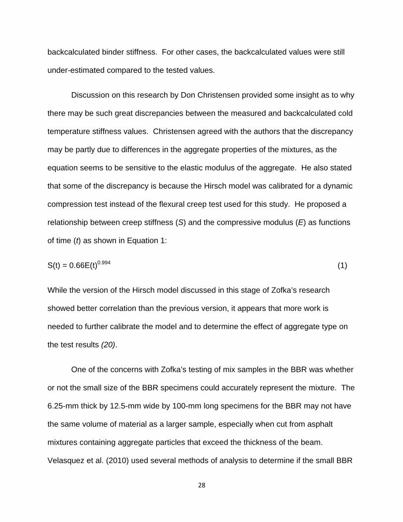
compression test instead of the flexural creep test used for this study. He proposed a
relationship between creep stiffness (S) and the compressive modulus (E) as functions
of time (t) as shown in Equation 1:
S(t) = 0.66E(t)0.994 (1)
While the version of the Hirsch model discussed in this stage of Zofka’s research
showed better correlation than the previous version, it appears that more work is
needed to further calibrate the model and to determine the effect of aggregate type on
the test results (20).
One of the concerns with Zofka’s testing of mix samples in the BBR was whether
or not the small size of the BBR specimens could accurately represent the mixture. The
6.25-mm thick by 12.5-mm wide by 100-mm long specimens for the BBR may not have
the same volume of material as a larger sample, especially when cut from asphalt
mixtures containing aggregate particles that exceed the thickness of the beam.
Velasquez et al. (2010) used several methods of analysis to determine if the small BBR
28

specimens could be used to accurately determine mixture stiffness at cold
temperatures. Ten laboratory mixes using four asphalt binder grades and two types of
aggregate were chosen for the study. Samples were compacted to 4% air voids using a
linear kneading compactor. Sets of three size beams were cut for each mix: 6.25 x
12.5 x 100-mm, 12.5 x 25 x 200-mm, and 18.75 x 37.5 x 300-mm. Each set of beams
was tested in 3 point bending at three temperatures based on the low-temperature
grade of the binder (low grade +22°C, low grade + 10°C, low grade -2°C). The two
larger sets of beams were tested using an MTS 810 servo hydraulic load frame. The
smaller set was tested using the BBR method described by Zofka.
Mix stiffness results at the high and intermediate-temperatures showed negligible
differences due to sample size. At the lower temperature, there was a more
pronounced difference in the results, especially for the smaller samples. The
researchers noted that the MTS device had issues with icing at this temperature level,
which could have caused error in the readings. Statistical analysis of the effects of size,
time, temperature, binder type, and aggregate on the creep stiffness at high and
intermediate-temperature showed that the only factor that did not have a statistical
influence on the creep stiffness was sample size. Low-temperature test results were
not included in the statistical analysis due to the icing issue.
Once the lack of effect of sample size was determined, the aggregate structure of
the different size samples was evaluated using digital imaging analysis and finite
element modeling. Based on the results of the study, it was determined that the
volumetric fraction and average size distribution of the aggregates were similar between
the three specimen sizes. Microstructural information was also found to be similar.
29
From these findings, the researchers concluded that the small-sized specimens tested
in the BBR could adequately represent the asphalt mixtures (21).
Bennert and Dongre (2010) evaluated the Hirsch model for backcalculating
asphalt binder properties (G*binder and δbinder) using E*mix data obtained from dynamic
modulus testing. Samples of loose plant mix were obtained and tested for E*mix
according to AASHTO TP 79-09, Determining the Dynamic Modulus and Flow Number
for Hot Mix Asphalt (HMA) Using the Simple Performance Test System. Samples of the
same plant mix were also extracted and the asphalt binder recovered. The recovered
asphalt binders were then tested in the DSR to determine their stiffness (G*binder) over a
range of temperatures and frequencies. The initial set of samples tested did not contain
any RAP. Without RAP in the mix, the backcalculated and tested results were expected
to be similar and give an indication of the validity of the method. For the
backcalculations, the researchers used a generalized logistic equation to create a
master curve of the E*mix data. The E*mix version of the Hirsch model was then used to
estimate the binder complex shear modulus, G*binder. The Christiansen-Anderson (CA)
model was used to create master curves of the backcalculated G*binder results and
compare them to the binder test results from the extracted binders. The estimated
G*binder data were then fit to the generalized logistic model and the constants obtained
from that equation used to estimate δbinder.
Once the researchers determined that a good correlation was possible between
the backcalculated binder data and actual tested binder results for mixes without RAP,
they explored ways to use the backcalculated results. One possibility was using the
backcalculated binder properties in the Mechanistic-Empirical Pavement Design Guide
30

(MEPDG) level 1 analysis. An MEPDG analysis on a mix with four RAP contents (0, 15,
20, and 25%) using binder properties obtained from the backcalculation procedure
showed reasonable rutting behavior with rut depth decreasing as RAP content
increased. Top-down cracking results did not rank as expected. A comparison
between G*binder results backcalculated from the plant mix at intermediate-temperatures
and the cracking resistance based on the Overlay Tester showed a good correlation
between the OT and the backcalculated G*binder resistance to reflection cracking (22).
A study by Tran et al. (2010) also evaluated the possibility of using the Hirsch
model to backcalculate the high-temperature properties of asphalt binders using mixture
dynamic modulus (E*mix) values. The researchers used HMA mixes sampled during the
2006 construction of the National Center for Asphalt Technology (NCAT) Pavement
Test Track. Mix specimens were tested for E*mix over a range of temperatures and
frequencies described in AASHTO TP62. The E*mix version of the Hirsch model was
used to backcalculate G*binder for the mixes. CA master curves were created for the
backcalculated G*binder values and the master curve parameters used to estimate δbinder.
Virgin binders sampled at the asphalt plant were RTFO aged and tested over a range of
temperatures and frequencies in the DSR to create master curves of binder stiffness.
The backcalculated G*binder values were compared to the tested G*binder values to
determine if the Hirsch model backcalculation method could accurately estimate the
high-temperature stiffness properties of the plant-produced mixes.
For the binders used in this study, the backcalculation procedure under-
estimated G*binder at the higher test temperatures. The δbinder values did not follow any
particular trend compared to the tested values and varied by as much as 10° high or
31

low. Backcalculated critical temperatures varied from the virgin binder critical
temperatures by anywhere from 0.5 to 15.1°C. The researchers recommended further
calibration of the Hirsch model to determine if individual calibrations for local materials
could improve the accuracy of the backcalculated data. It was suggested that different
calibrations for laboratory and plant-produced mixes may also be necessary (23)
Swiertz et al. (2011) conducted a study to evaluate a proposed method of
estimating the low-temperature properties of HMA blends containing RAP and
reclaimed asphalt shingles (RAS). The proposed method consisted of testing three sets
of BBR test specimens prepared as follows:
1. Virgin binder tested using standard BBR procedure as described in AASHTO
T313,
2. Mortar made from RAP passing the No. 50 sieve and retained on the No. 100
sieve (designated SRAP), and
3. Mortar made from SRAP aggregate recovered using an ignition furnace,
blended with RTFO aged virgin binder at a binder content equal to that of the
SRAP (designated RRAP).
The two sets of mortar samples were tested at temperatures corresponding to the low-
temperature grade of the virgin binder and the difference between the SRAP and RRAP
properties for BBR (stiffness (S) and m-value) were calculated. Since the aggregate
and binder contents were the same for both sets of specimens, the difference between
the test results was theorized to be due solely to the increased stiffness of the RAP
binder. This difference was used to shift the virgin binder test results to provide an
32

estimate of the RAP binder properties. The estimated RAP binder properties were then
used along with the virgin binder properties to create blending charts for estimating the
effect of adding different percentages of RAP to HMA. Additional work was done to
determine if the same shifting procedure could be applied to testing low-temperature
fracture energy properties using the single-edge notched beam (SENB) test. For this
test, specimens were created in a similar manner as before with the addition of a 3-mm
notch in the width of the BBR side mold. Materials tested included one RAP source
blended with two virgin binders and one RAS source blended with one virgin binder.
Samples were tested at -6, -12, and -18°C to measure stress intensity factor KIC and
fracture energy, with the load and displacement at failure also reported.
Artificially created RAP [virgin binder aged through two cycles of long-term aging
in the pressure-aging vessel (PAV) blended with RAP aggregate recovered using the
ignition oven] was used to verify the ability of the proposed method to identify the low-
temperature binder properties of HMA containing RAP. The artificial RAP was blended
with two virgin binders (PG 64-22 and PG 58-28) at 15 and 25%. The blends were
tested using the proposed procedure and the estimated low-temperature properties
were compared to BBR test results on binders created by blending the virgin and
artificially aged RAP binder. It was found that the proposed procedure could estimate
the low-temperature properties of the artificial RAP blends within 1°C of the tested
values. When the proposed procedure was used to estimate the low-temperature
properties using combinations of actual RAP materials (4 sources) and virgin binder
(PG 64-22 and PG 58-28), it was shown that the interaction of RAP and virgin binder
was different for different combinations of materials. This would imply that the current
33

tiered approach to RAP blends may not be valid for all materials. It also implied that an
assumed constant rate of change for continuous grade per percent of RAP binder
replacement may not be valid for every RAP and virgin binder combination. The
procedure worked for RAS materials as well as RAP binders and allowed for the
estimation of the low-temperature properties of blends containing both RAP and RAS
materials. SENB testing could detect changes in the mixture fracture energy of the
asphalt mixtures due to the addition RAP and RAS materials but more work will be
needed to define what the differences mean (24).
Summary of Key Findings
Key findings from the literature review are listed as follows:
1. RAP binders are typically characterized using one of the available combinations
of solvent extraction and recovery procedures. While these procedures provide
recovered RAP binder to test, the binder properties are affected by the process.
Solvents affect recovered RAP binder properties through chemical hardening,
retained solvent, or both. The amount of time needed to complete the extraction
/ recovery process can also affect the binder as can the temperature at which the
procedure is performed (7, 9, 10).
2. Linear blending charts created using the properties obtained from Superpave
performance testing of the virgin and recovered RAP binders are the current
method of choice for characterizing asphalt mixtures containing more than 25%
RAP. While much work has been done to validate the use of these charts, it is
noted that they have limitations (6, 11,12).
34

3. Blending charts assume full blending between RAP and virgin binders as well as
linear behavior with increasing RAP content. This may not be the case and could
lead to inaccurate estimation of the binder properties of RAP mixtures (6, 11, 12).
4. RAP mix designs with high percentages of RAP can provide acceptable
performance if aggregate and binder properties are properly characterized and
accounted for (6, 12, 13, 14, 15, 17).
5. Researchers have not achieved a clear understanding of how much blending
occurs between virgin and RAP binder in HMA. Studies have determined that
there is some degree of blending of the binders, but that the amount of blending
varies. Factors that may influence the amount of blending include RAP content,
virgin binder stiffness, and mixture handling. Lack of precision in characterizing
binders recovered from RAP and RAP mixtures makes studying this topic difficult
(6, 15).
6. The addition of RAP to HMA mixes increases the high-temperature stiffness of
HMA. The amount of stiffening increases with increasing RAP content, with
higher RAP content mixes being significantly stiffer than virgin mixes. Lower
RAP contents may or may not be significantly stiffer at high-temperatures than
virgin mixes. Research on this behavior illustrates the need to account for the
RAP binder in HMA mixes containing high percentages of RAP (typically >25%)
and supports the current AASHTO M323 tiered approach to accounting for RAP
binder based on RAP content (6, 12, 13, 14, 15, 16, 17).
35

7. Although it was expected that the addition of RAP would decrease the fatigue life
of HMA mixes, this was not always the case. Some research showed that mixes
with up to 40% RAP showed an improved fatigue life. Other research showed
the expected decrease in fatigue resistance for higher RAP content mixes. In
cases where the fatigue life decreased with the addition of RAP, changing to a
softer virgin binder grade as recommended in AASHTO T323 lessened the effect
(6, 16).
8. As with the fatigue life, increased RAP content is expected to decrease the cold
temperature cracking resistance of HMA mixes. The research shows that this
does occur, but the change is usually much smaller than the effect on the high-
temperature properties. Some of the research indicated that mixes containing up
to 40% RAP still provided acceptable low-temperature properties compared to
the virgin mixes. It was also shown that reducing the stiffness of the virgin binder
improved the low-temperature properties of the RAP mixes (6, 14, 15, 16).
9. Use of the Hirsch model to backcalculate binder stiffness as a function of tested
mixture E*mix was explored and found to be a potential method for characterizing
the binder properties of asphalt mixtures. Recent research shows that the Hirsch
model has a tendency to under-estimate G*binder and has difficulty estimating
δbinder. It is possible that further calibration of the model will improve the
correlation (22, 23).
10. Work has been done to identify ways to test mixture stiffness in the laboratory to
obtain the inputs needed for the Hirsch model. Research in this area has
36

primarily focused on creating a specimen to test in existing binder testing
equipment such as the BBR. Success has been limited by the difficulty obtaining
of representative a test specimen small enough to fit into the test equipment and
by the need to calibrate the models to reflect the differences between binder and
mixture testing methods (19, 20, 21, 24).
EXPERIMENTAL PLAN
The mixture test chosen for evaluation in this study was a mixture torsion bar test
similar to the one described in ASTM D7552-09, Determining the Complex Shear
Modulus (G*mix) of Bituminous Mixtures Using Dynamic Shear Rheometer. The torsion
bar procedure was developed by Gerry Reinke at Mathy Construction Co. This test was
chosen because of its small sample size and ability to be performed on the DSR, an
existing piece of binder testing equipment, with commercially available fixtures. The
test provides a measure of mixture complex shear modulus (G*mix) over a range of
frequencies and can easily be run at multiple temperatures, allowing for the creation of
master curves of mixture stiffness. This section includes a discussion of the test
materials and procedures used to evaluate the DSR torsion bar procedure.
Materials
The following is a description of the materials used to evaluate the DSR torsion
bar procedure. The materials tested included mixes containing only virgin components
(asphalt binder and aggregate), mixes containing only RAP materials, HMA mixes
designed at multiple RAP contents, and plant-produced mixes containing RAP.
37
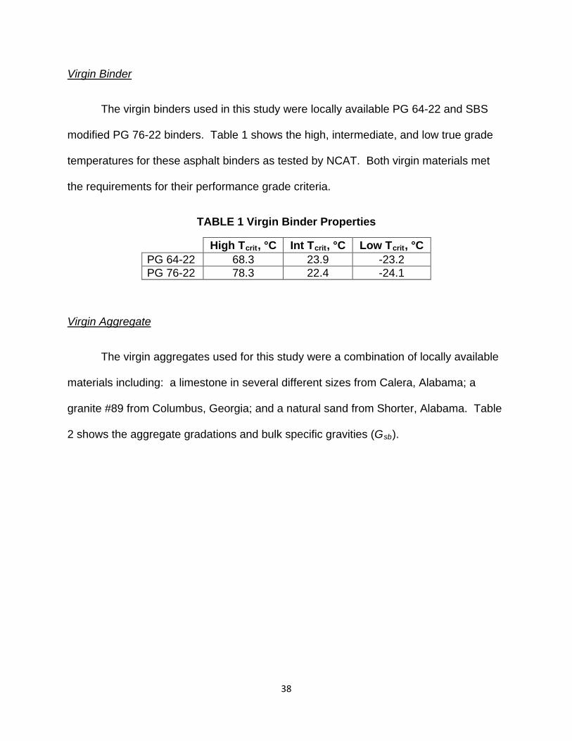
Virgin Binder
The virgin binders used in this study were locally available PG 64-22 and SBS
modified PG 76-22 binders. Table 1 shows the high, intermediate, and low true grade
temperatures for these asphalt binders as tested by NCAT. Both virgin materials met
the requirements for their performance grade criteria.
TABLE 1 Virgin Binder Properties
High Tcrit, °C Int Tcrit, °C Low Tcrit, °C PG 64-22 68.3 23.9 -23.2 PG 76-22 78.3 22.4 -24.1
Virgin Aggregate
The virgin aggregates used for this study were a combination of locally available
materials including: a limestone in several different sizes from Calera, Alabama; a
granite #89 from Columbus, Georgia; and a natural sand from Shorter, Alabama. Table
2 shows the aggregate gradations and bulk specific gravities (Gsb).
38

TABLE 2 Virgin Aggregate Gradation
Percent Passing, % Limestone Granite Shorter
Sand Sieve Size, mm #89 #67 #7 #820 #89 50 100 100 100 100 100 100
37.5 100 100 100 100 100 100 25 100 100 100 100 100 100 19 100 100 100 100 100 100
12.5 100 84.2 97.1 100 100 100 9.5 99.5 50.2 74.4 100 99.5 100 4.75 37.5 10.3 15.2 96.7 27.1 100 2.36 8.2 2.6 1.9 61.7 3.3 94.6 1.18 3.2 1.5 1.2 38.3 1.6 79.5 0.6 2.0 1.3 1.0 25.2 1.6 51.4 0.3 1.7 1.3 1.0 17.8 1.6 21.7 0.15 1.6 1.3 1.0 13.0 1.6 5.2
0.075 1.5 1.2 0.9 10.1 1.6 0.9 Gsb 2.645 2.746 2.717 2.646 2.61 2.656
RAP Materials
Five Alabama RAP sources were evaluated and designated as RAP 1 through
RAP 5 for reference purposes. Table 3 shows the supplier information, designations,
aggregate gradations (% passing each sieve size), asphalt contents, and specific
gravities for each of the RAP sources as received. A map showing the supplier
locations is included in Appendix A. Gradations and specific gravities were evaluated
on aggregates recovered from the RAPs by solvent extraction (ASTM D2172, Method
A) using trichloroethylene. The maximum theoretical specific gravity (Gmm) and
aggregate bulk specific gravity (Gsb) were required to calculate the volumetric properties
of the test specimens. Gmm was determined using AASHTO T209, Theoretical
Maximum Specific Gravity and Density of Hot Mix Asphalt. The aggregate bulk specific
39

gravities (Gsb) were determined using either AASHTO T84, Specific Gravity and
Absorption of Fine Aggregate, or AASHTO T85, Specific Gravity and Absorption of
Coarse Aggregate.
TABLE 3 RAP Properties
RAP
Wiregrass Const.
Co.
East Alabama Paving
McCartney Const. Co.
S.T. Bunn Const. Co APAC
Sieve Size, mm 1 2 3 4 5 25.0 100.0 100.0 100.0 100.0 100.0 19.0 100.0 100.0 100.0 97.7 100.0 12.5 99.8 95.6 99.9 90.7 97.4 9.5 95.4 85.8 95.7 84.1 88.3 4.75 71.4 65.6 62.3 65.3 62.9 2.36 58.1 53.0 38.0 47.1 40.5 1.18 46.9 42.9 23.0 35.8 23.7
0.600 32.9 32.4 14.3 28.0 12.1 0.300 20.4 21.8 8.0 17.1 5.5 0.150 12.3 14.5 4.4 9.7 3.3 0.075 8.5 9.5 2.9 7.2 2.2 % AC 5.2 4.7 4.7 4.7 4.6 Gmm 2.476 2.52 2.548 2.511 2.487 Gmb 2.573 2.647 2.748 2.61 2.719
The gradations shown in Table 3 were based on the as-received RAP materials. RAP 3
had been fractionated over a 4.75-mm sieve at the plant. RAP materials from the other
sources did not indicate any processing prior to their arrival at NCAT.
Mix Designs
Mix designs were created using both the virgin and RAP materials. These
blends were used to determine if the torsion bar procedure could detect changes in
40
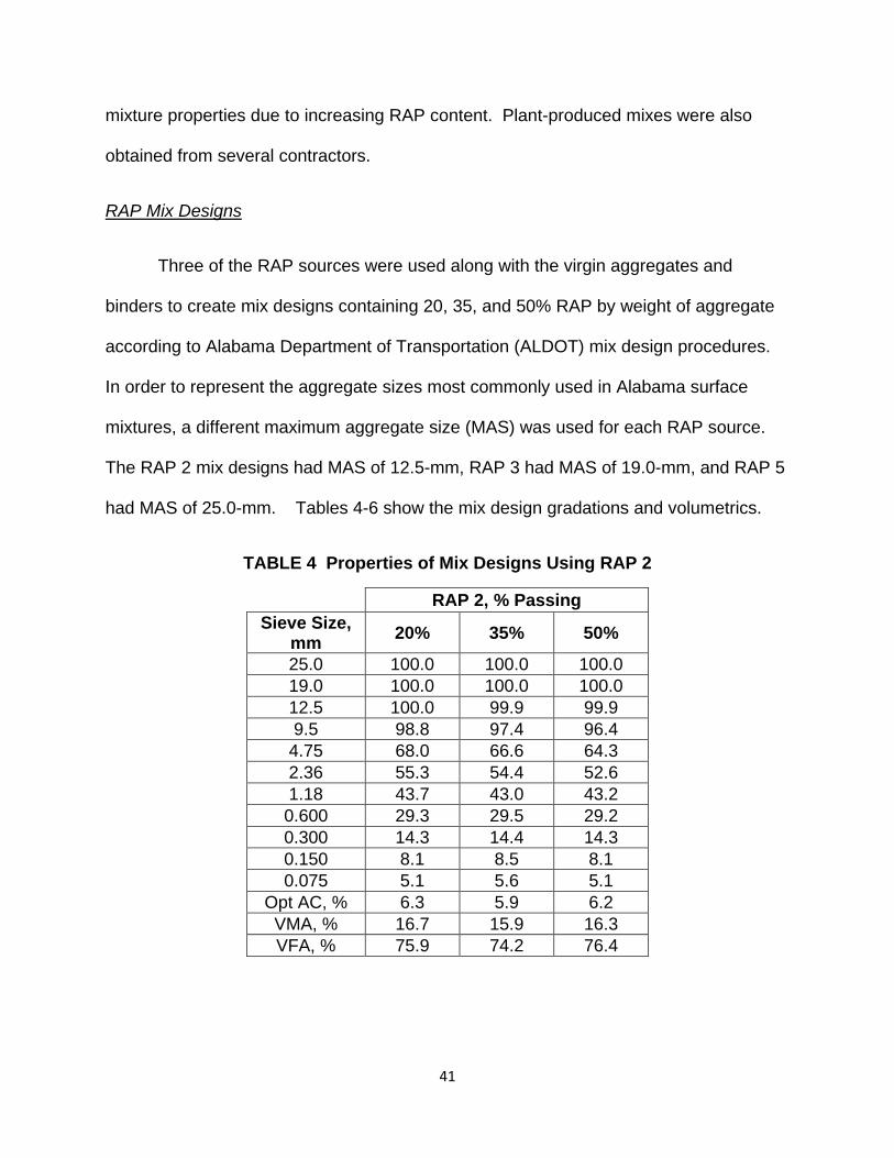
mixture properties due to increasing RAP content. Plant-produced mixes were also
obtained from several contractors.
RAP Mix Designs
Three of the RAP sources were used along with the virgin aggregates and
binders to create mix designs containing 20, 35, and 50% RAP by weight of aggregate
according to Alabama Department of Transportation (ALDOT) mix design procedures.
In order to represent the aggregate sizes most commonly used in Alabama surface
mixtures, a different maximum aggregate size (MAS) was used for each RAP source.
The RAP 2 mix designs had MAS of 12.5-mm, RAP 3 had MAS of 19.0-mm, and RAP 5
had MAS of 25.0-mm. Tables 4-6 show the mix design gradations and volumetrics.
TABLE 4 Properties of Mix Designs Using RAP 2
RAP 2, % Passing Sieve Size,
mm 20% 35% 50%
25.0 100.0 100.0 100.0 19.0 100.0 100.0 100.0 12.5 100.0 99.9 99.9 9.5 98.8 97.4 96.4
4.75 68.0 66.6 64.3 2.36 55.3 54.4 52.6 1.18 43.7 43.0 43.2 0.600 29.3 29.5 29.2 0.300 14.3 14.4 14.3 0.150 8.1 8.5 8.1 0.075 5.1 5.6 5.1
Opt AC, % 6.3 5.9 6.2 VMA, % 16.7 15.9 16.3 VFA, % 75.9 74.2 76.4
41
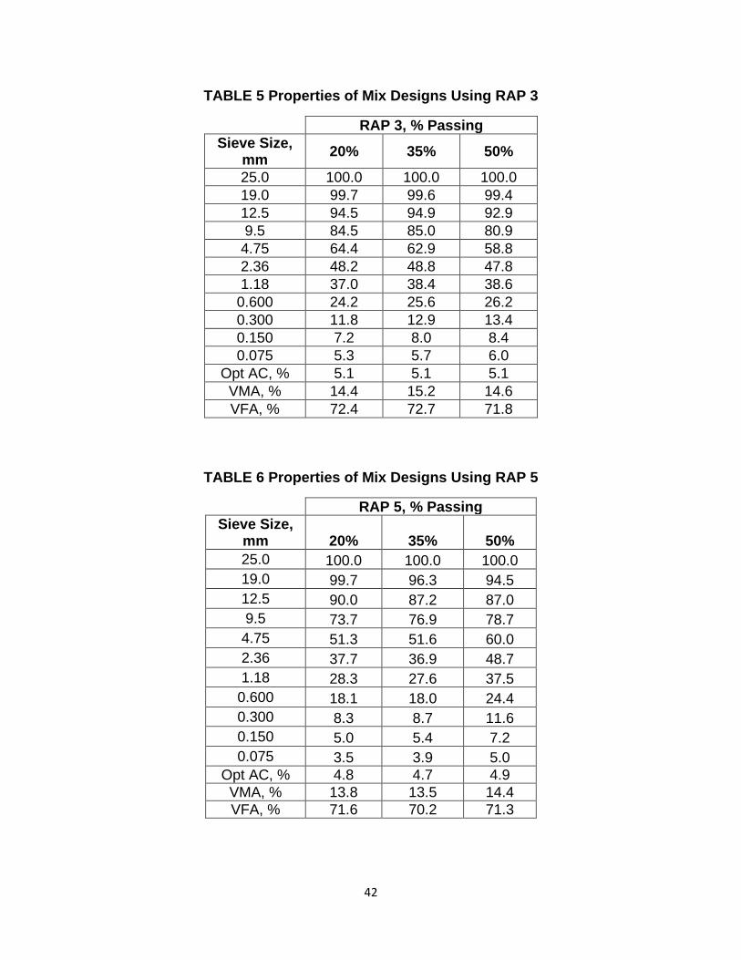
TABLE 5 Properties of Mix Designs Using RAP 3
RAP 3, % Passing
Sieve Size, mm 20% 35% 50%
25.0 100.0 100.0 100.0 19.0 99.7 99.6 99.4 12.5 94.5 94.9 92.9 9.5 84.5 85.0 80.9 4.75 64.4 62.9 58.8 2.36 48.2 48.8 47.8 1.18 37.0 38.4 38.6
0.600 24.2 25.6 26.2 0.300 11.8 12.9 13.4 0.150 7.2 8.0 8.4 0.075 5.3 5.7 6.0
Opt AC, % 5.1 5.1 5.1 VMA, % 14.4 15.2 14.6 VFA, % 72.4 72.7 71.8
TABLE 6 Properties of Mix Designs Using RAP 5
RAP 5, % Passing
Sieve Size, mm 20% 35% 50% 25.0 100.0 100.0 100.0 19.0 99.7 96.3 94.5 12.5 90.0 87.2 87.0 9.5 73.7 76.9 78.7 4.75 51.3 51.6 60.0 2.36 37.7 36.9 48.7 1.18 28.3 27.6 37.5
0.600 18.1 18.0 24.4 0.300 8.3 8.7 11.6 0.150 5.0 5.4 7.2 0.075 3.5 3.9 5.0
Opt AC, % 4.8 4.7 4.9 VMA, % 13.8 13.5 14.4 VFA, % 71.6 70.2 71.3
42

Plant-Produced Mix
Samples of plant-produced mixes containing RAP were obtained from local
contractors. Table 7 shows the job mix formula information for these mixes. These
materials were given alphabetical designations to distinguish them from the 100% RAP
materials and laboratory mix designs. Gradations, RAP contents, recycled asphalt
shingle (RAS) contents, asphalt binder contents, and virgin asphalt binder grades were
all obtained from the job mix formulas provided by the contractors supplying the mixes.
TABLE 7 Plant Mix Information
Plant Mix
McCartney Const. Co.
S.T. Bunn Const. Co.
Dunn Const Co.
Mobile Asphalt
Co.
East Alabama
Paving Co. Sieve Size,
mm A B C D E 50 100 100 100 100 100
37.5 100 100 100 100 100 25 100 100 100 100 100 19 84 96 100 99 90
12.5 63 81 90 87 77 9.5 54 72 70 78 67
4.75 45 54 57 56 45 2.36 31 44 44 41 37 1.18 20 37 33 33 29 0.6 14 28 24 26 19 0.3 10 14 13 13 11
0.15 7 9 9 6 7 0.075 4.5 5.2 5.6 3.5 4.4
% RAP 25 15 + 5%
RAS 10 + 5%
RAS 20 20 Virgin Binder
Grade 76-22 64-22 64-22 76-22 64-22 %AC 4.2 5 5.3 4.5 4.5
43

Organization of the Testing Plan
Binder Tests
The first part of this study included characterizing the virgin and recovered RAP
binders used in the study. The virgin PG 64-22 and PG 76-22 binders were tested in
accordance with AASHTO M320-05, Performance Graded Asphalt Binder, and
AASHTO R29-08, Grading or Verifying the Performance Grade (PG) of an Asphalt
Binder to determine their PG and true binder grades. Specific binder tests in this
methodology include:
• viscosity measurements using the Rotational Viscometer (RV) procedure
described in AASHTO T316-06,
• short-term aging using the Rolling Thin Film Oven (RTFO) procedure
described in AASHTO T240-08,
• long-term aging using the Pressure Aging Vessel (PAV) procedure described
in AASHTO R28-06,
• binder complex shear modulus (G*binder) and phase angle (δbinder) using the
Dynamic Shear Rheometer (DSR) at high and intermediate-temperatures, as
described in AASHTO T315-08,
• binder frequency sweeps using the DSR to determine G*binder at different
temperatures and frequencies, and
44

• low-temperature stiffness and relaxation properties from the Bending Beam
Rheometer (BBR), as described in AASHTO T313-12.
Critical temperatures are defined as the temperature at which a test criterion is met (for
example, the critical temperature for unaged DSR is the temperature at which G*/sin(δ)
= 1.00 kPa) and are determined by interpolating between two test results that bracket
the criteria. The high critical temperature, Tcrit, High, is based on the lower of the
unaged and RTFO-aged DSR results. The low critical temperature, Tcrit, Low, is based
on the warmer of the two BBR results (S and m-value). The intermediate critical
temperature, Tcrit, Int, is based on the results from the PAV-aged DSR. The true-grade
of an asphalt binder is determined from the critical temperatures and is rounded to a
standard grade to determine the PG grade (25). Table 8 shows a summary of the
binder tests and the criteria associated with them.
TABLE 8 Binder Testing Summary
Test AASHTO Method Output Criteria
RV T316 Viscosity (Pa-S) Viscosity ≤ 3.0 Pa-S
DSR T315 G* (kPa) and δ (degrees)
Unaged Binder: G*/sin(δ) ≥ 1.00 kPa RTFO Aged Binder: G*/sin(δ) ≥ 2.20 kPa PAV aged binder: G*sin(δ) ≤ 5,000 kPa
BBR T313 S (Mpa) and m-value (no units)
S ≤ 300 Mpa m-value ≥ 0.300
RTFO T240 Mass Change, % Mass change ≤ 1.00%
PAV R28 aged asphalt binder for further testing
no criteria
45

Asphalt binder was extracted and recovered from samples of each of the RAP
sources and plant produced mixes using the centrifuge extraction method (ASTM
D2172-05 Method A) with TCE as the solvent. The rotary evaporator recovery
procedure (ASTM D5404-03) was used to remove the solvent from the extracted binder.
At least two replicate samples were recovered for each RAP source. Only one sample
was recovered for the plant mixes.
The recovered binders were tested to determine their PG and true-grade
temperatures. When testing recovered binders, short-term aging in the RTFO is not
required. Recovered binder has already been through the mixing and construction
phase simulated by the short-term aging procedure and, therefore, does not need
further aging. Some agencies use the RTFO aging procedure for their recovered
binders as a means of assuring that all the solvent from the extraction/recovery process
is removed. Since this is not a standardized procedure and does cause additional aging
of the recovered binder, it was not done as part of this testing. The recovered binders
were long-term aged because this seemed necessary to provide accurate intermediate
and low PG grade temperatures. Binder tests on extracted/recovered binder have long
been the preferred method of characterizing RAP binder and are used as the basis for
creating blending charts for high RAP mixtures. Consequently, it was felt that recovered
binder properties should be used as the benchmark for this project to determine the
ability of the chosen model to accurately predict binder stiffness.
46

Mixture Tests
The mixture test chosen for this project was a torsion bar procedure tested using
small bars of mix in the DSR. At the time the testing took place, ASTM D7552 was not
an official ASTM standard so modifications were made to the test procedure (mainly
sample size and test temperature) and are noted below. The test procedure uses a
torsional rectangular geometry (torsion bar) to measure the complex shear modulus
(G*mix) of a small sample of asphalt mixture at multiple temperatures and frequencies.
The torsion bars used for this procedure were cut from samples that had been
compacted using the Superpave Gyratory Compactor (SGC). For the 100% virgin
samples, four sets of test specimens were compacted:
1. PG 64-22 with limestone 820s screened over a #4 sieve,
2. PG 64-22 with limestone 820s screened over a #8 sieve,
3. PG 76-22 with limestone 820s screened over a #4 sieve, and
4. PG 76-22 with limestone 820s screened over a #8 sieve.
After mixing, the mixes were short-term oven-aged for 2 hours at 150°C and
compacted using the SGC. The 100% RAP torsion bars were comprised of RAP with
no virgin materials. The RAP materials were heated in the oven, mixed, then allowed to
age for an additional hour at 150°C before being compacted. ASTM D7552 does not
provide guidance about compactive effort and states that the use of discarded
volumetric specimens is acceptable. Because another portion of this project required
the compaction of gyratory specimens for mixture performance testing to an air void
47

level of 7%, the rejected performance specimens were used to cut the torsion bar test
specimens. Therefore, the compacted specimens used for this testing were compacted
to somewhere between 5-7% air voids. The cut test specimens had air voids that were
higher than those of the compacted samples and average values ranged from 7.0 to
11.2% for the virgin and 100% RAP test specimens.
Once compacted, the samples were sliced into small chunks taken from the
middle of the compacted specimen. A Master Tiler diamond wheel 7-in. wet saw
(Figure 1) was used to further slice the samples into 5.5-mm thick by 11.5-mm wide by
50-mm long bars (Figure 2). This was a change from D7552; the 9 ± 1.5-mm thick by
12 ± 2-mm wide by 49 ± 2-mm long dimension specified in ASTM D7552 was too stiff
and maxed out the torque capacity of the DSR at high frequencies and cold
temperatures.
Figure 1 Saw Used to Cut Torsion Bar Specimen
48

Figure 2 Torsion Bar Specimen
After cutting, the torsion bars were measured (length, width, and thickness in
mm) and weighed (grams) to calculate bulk specific gravity (Gmb) and air voids using
dimensional analysis calculations, as shown in Equation 2.
ThicknessWidthLengthWeightcmgDensity
**1000*)/(, 3 =
(2)
The air voids of the sample were calculated using Equation 3.
100*%mm
mm
GDensityGAirVoids −
= (3)
Several specimens were cut for each group of materials and narrowed down to
four replicate test specimens per group. The final test specimens were selected to be
within approximately 1% air voids of each other. Care was also taken to select bars that
did not vary more than 1 mm from end to end for width or thickness. Finally, the bars
were inspected to make sure they did not have any imperfections or roughness at the
ends that might interfere with the clamping assembly.
49

A TA Instruments AR2000 EX DSR with a rectangular solid clamp set-up and
environmental temperature chamber with liquid nitrogen hookup for temperature control
was used to test the torsion bar samples (Figures 3-4). Before testing, the gap between
the clamping fixtures was zeroed at the mid-range of test temperatures. The
environmental chamber was opened, and the test specimen was placed in the clamping
fixture at ambient temperature. The clamp screws were finger-tightened and the bar
visually inspected to ensure it was straight and centered in the fixture. A torque wrench
was used to tighten the screws to a torque of approximately 20 dynes, being careful not
to introduce a normal load on the specimen as indicated by the DSR software.
Figure 3 DSR Rectangular Torsion Clamps
50

Figure 4 AR2000EX Torsion Bar Testing Setup
Figure 5 Torsion Bar Loading
After clamping the specimen, the environmental chamber was closed and
allowed to equilibrate to the lowest test temperature ± 0.1°C for at least 15 minutes.
The testing was conducted in controlled strain mode using a strain of 0.01%. At this
strain, ten frequencies ranging from 0.01 to 10 Hz were applied to the bar by oscillating
the top clamp in a sinusoidal fashion as shown in Figure 5. Each frequency was tested
for a total of 20 cycles. For each cycle, measurements of the shear stress required to
51

maintain the required frequency and strain level were taken. This stress was used to
calculate G*mix for each cycle as shown in equation 4.
rainMaxShearStressMaxShearStG mix =* (4)
The time lag in seconds between sample loading and movement was also measured
and used to calculate δmix as shown in equation 5.
frequencytimemix **360=δ (5)
For each frequency, the first 10 cycles of data were discarded, and the results of the
second 10 were averaged for the final result. Testing was repeated at five test
temperatures (20, 30, 40, 50, and 60°C) to provide multiple isotherms of G*mix and
frequency. These temperatures were chosen instead of the high PG grade
temperature required by the climate (64°C for Alabama) recommended in ASTM D7552
because of issues with the mix samples deforming at the warmer temperature.
Description of Models and Master Curves
Models
Many researchers working to improve characterization of high-temperature RAP
properties have focused on developing a mixture test (i.e., dynamic modulus) to obtain
a mixture stiffness parameter to estimate binder stiffness. Conversely, several models
currently exist for calculating mixture stiffness based on tested binder stiffness. In
theory these models could be used with known mixture stiffness to backcalculate binder
stiffness.
52

The first predictive models for mixture stiffness were developed in the late 1970s
when Witczak began his work developing several versions of a model to predict mixture
Dynamic Modulus, E*mix, using such parameters as binder viscosity, aggregate
gradation, testing frequency, volume of air voids, and volume of effective binder. While
the models were all able to predict E*mix reasonably well, earlier versions had several
limitations:
• Mixtures with modified asphalt were omitted from model calibration,
• The binder viscosity value used in the models was based on asphalt viscosity or
penetration at 25°C only and assumed that the laboratory aging approximated
field aging, and
• The models were based on a polynomial form and did not provide accurate
predictions at extremely hot or cold conditions.
A version of the Witczak model developed in the 2006 attempted to address these
concerns by including the Superpave binder properties G*binder and phase angle
(δbinder), that could be based on test results at any temperature or aging condition
desired. The form of the model was changed from a basic polynomial equation to a
symmetrical sigmoidal function in order to improve prediction at the extreme values.
The final model is shown in Equation 6.
53

[ ]
( )
+
−−+
+++
+
+−−−+−++−
+−=
+−−
−
inderbinder bG
beffa
aa
beffa
beffa
bmix
e
pppVV
VV
VVV
vpppppp
GE
δlog8834.0*log(5785.07814.0
3423838
23838
244
2200200
0052.0
1
01.00001.0012.071.003.056.2
06.108.000014.0006.00001.0011.00027.0032.065.6
**754.0349.0*log
(6)
Where:
E*mix = asphalt mix dynamic modulus, in 105 psi;
G*binder = dynamic shear modulus of binder, psi;
δbinder = phase angle of binder associated with G*b, degree;
F = load frequency, in Hz;
Va = percent air voids in the mix, by volume;
Vbeff = percent effective bitumen content, by volume;
P34 = percent retained on ¾-in sieve, by total aggregate weight (cumulative);
P38 = percent retained on the 3/8-in sieve, by total aggregate weight (cumulative);
P4 = percent retained on No.4 sieve by total aggregate weight (cumulative); and
P200 = percent passing No. 200 sieve, by total aggregate weight.
This version of the Witczak model was found to have excellent statistical
correlation based on the database used for its development. The use of the actual
binder properties gave it greater flexibility for estimating E*mix at various temperatures
and aging conditions. The nonlinear sigmoidal function also provided better results at
high and low-temperatures (26).
54
Another model frequently used for estimating asphalt mixture modulus (shear or
dynamic) from the results of asphalt binder complex shear modulus (G*binder) testing and
mixture volumetric analysis was developed in the early 2000s by Christiansen et al.
Several variations of an existing version of the law of mixtures, the Hirsch Model, were
evaluated before a final, simple model was chosen. The final version of the model
estimates the asphalt mixture modulus directly from the asphalt binder complex shear
modulus, the voids in the mineral aggregate (VMA) of the mixture, and the voids filled
with asphalt (VFA) of the mixture. The model takes two forms: one for dynamic
complex shear modulus, G*mix, and one for dynamic complex extensional modulus,
E*mix. Equations 7 - 10 show both forms of the finalized model.
55
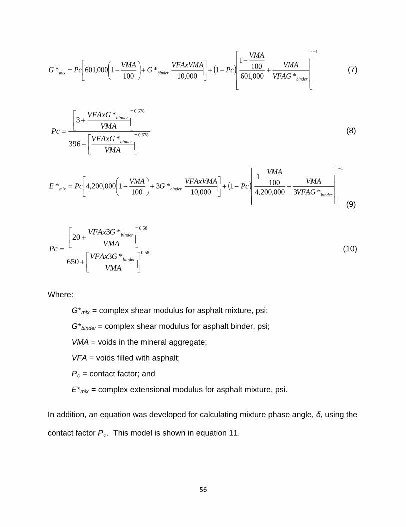
( )
1
*000,601100
11
000,10*
1001000,601*
−
+−
−+
+
−=
binderbindermix VFAG
VMAVMA
PcVFAxVMAGVMAPcG (7)
678.0
678.0
*396
*3
+
+
=
VMAVFAxG
VMAVFAxG
Pcbinder
binder
(8)
( )
1
*3000,200,4100
11
000,10*3
1001000,200,4*
−
+−
−+
+
−=
binderbindermix VFAG
VMAVMA
PcVFAxVMAGVMAPcE
(9)
58.0
58.0
*3650
*320
+
+
=
VMAGVFAx
VMAGVFAx
Pcbinder
binder
(10)
Where:
G*mix = complex shear modulus for asphalt mixture, psi;
G*binder = complex shear modulus for asphalt binder, psi;
VMA = voids in the mineral aggregate;
VFA = voids filled with asphalt;
Pc = contact factor; and
E*mix = complex extensional modulus for asphalt mixture, psi.
In addition, an equation was developed for calculating mixture phase angle, δ, using the
contact factor Pc. This model is shown in equation 11.
56

( ) 6.9)log(39)log(5.9 2 +−−= PcPcδ (11)
Model verification was completed by estimating mixture shear modulus (G*mix) for
tests performed during the SHRP program. These calculations showed the agreement
between predicted and measured values of G*mix, though good, were slightly under-
predicted, while the phase angle prediction was less accurate, especially at higher
phase angles. Model calculations were also compared to Witczak’s model and had
similar accuracy for the data used, although it was theorized that this level of agreement
would not always be the case. A comparison using binder creep modulus data from the
BBR in the Hirsch model showed that when compared to the mixture creep compliance
results from SHRP, the Hirsch model tended to under estimate mixture values (27).
The Hirsch model for G*mix shown in equations 7 and 8 was chosen as the
starting point for the high and intermediate-temperature backcalculation testing for this
project. This model was chosen over the Witczak model due to its simple form and use
of a single, easily tested binder parameter (G*binder). For the first step in the analysis of
the test results, the G*binder values from the tested virgin and recovered RAP binder
frequency sweeps were used with the Hirsch model to calculate G*mix for the individual
torsion bar samples (forward-calculation). In order to obtain replicate results so that
statistical analysis could be performed, values of VMA and VFA were calculated from
the dimensional analysis of the torsion bar samples and each set of values used to
calculate a value of G*mix. The calculated G*mix values were compared to those
obtained from the torsion bar mixture testing and analyzed to determine the model’s
ability to accurately estimate the torsion bar mixture stiffness.
57

Once it was determined that the Hirsch model could accurately forward-calculate
mixture stiffness, a Microsoft Excel® spreadsheet was used to iteratively solve for the
binder stiffness using mixture stiffness values measured using the torsion bar test
procedure. Backcalculations were done for G*binder at each of the temperature-
frequency combinations tested during the torsion bar test so that master curves of the
backcalculated binder data could be created. The same VMA and VFA values as
before were used for this process so that replicate test results could be obtained. A
complete example of the backcalculation procedure is included in Appendix B.
Master Curves
To obtain G*binder values at the temperatures and frequencies necessary for
accurately estimating the true and PG binder grades from the backcalculated binder
stiffness results it was necessary to construct master curves. Master curves help define
both time dependency (the location and shape of the master curve) and temperature
dependency (shift factors) of a material and allow for determination of stiffness
properties at temperature and frequencies that are not easily tested in a laboratory
setting. Figure 6 shows an example of a master curve for complex shear modulus,
G*binder.
58
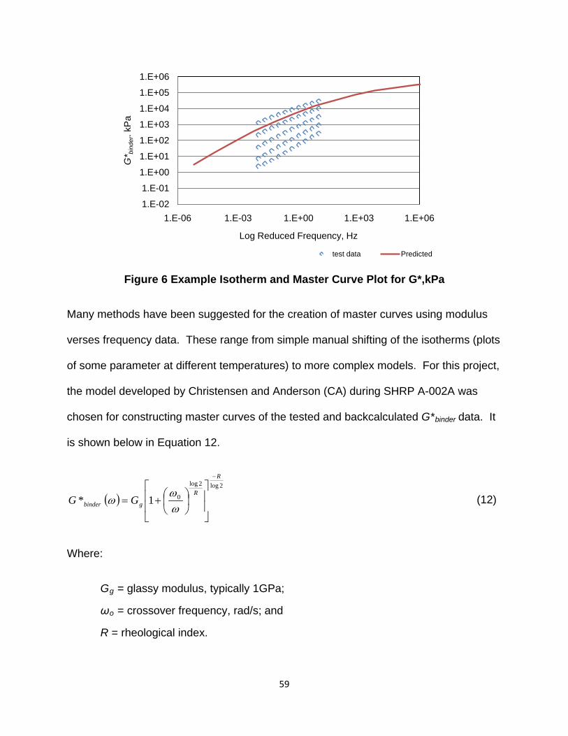
Figure 6 Example Isotherm and Master Curve Plot for G*,kPa
Many methods have been suggested for the creation of master curves using modulus
verses frequency data. These range from simple manual shifting of the isotherms (plots
of some parameter at different temperatures) to more complex models. For this project,
the model developed by Christensen and Anderson (CA) during SHRP A-002A was
chosen for constructing master curves of the tested and backcalculated G*binder data. It
is shown below in Equation 12.
( )2log2log
01*
R
R
gbinder GG
−
+=ωω
ω (12)
Where:
Gg = glassy modulus, typically 1GPa;
ωo = crossover frequency, rad/s; and
R = rheological index.
1.E-02
1.E-01
1.E+00
1.E+01
1.E+02
1.E+03
1.E+04
1.E+05
1.E+06
1.E-06 1.E-03 1.E+00 1.E+03 1.E+06
G* b
inde
r. kP
a
Log Reduced Frequency, Hz
test data Predicted
59

The shift factors used to manipulate the G* isotherms to a reference temperature (25°C
for this project) were defined using the Williams-Landel-Ferry (WLF) equation for
temperatures above the reference temperature and the Arrhenius equation for
temperatures below the reference temperature. The shift factor equations are shown in
Equations 13 and 14.
)()(
)()(log
2
1
r
r
r TTCTTC
TaTa
−+−−
=
(13)
Where:
a(T)/a(Tr) = WLF shift factor relative to the reference temperature;
C1, C2 = empirically determined constants;
T = Selected temperature, in °C or °K; and
Tr = Refining temperature, in °C or °K.
−
=
r
a
r
TTR
ETaTa
11303.2
)()(log
(14)
Where:
a(T)/a(Tr) = Arrhennius shift factor relative to the reference temperature;
Ea = Activation energy for flow below Tr; and
R = Ideal gas constant = 8.34 J/mol -°K.
The phase angle, δ, was determined from the master curves relative to frequency using
Equation 15 (28).
60

+
=R
2log
0
1
90)(
ωω
ωδ (15)
A master curve model developed by Rowe and Sharrock and shown in equation
16 was chosen for creating master curves for mixture stiffness results.
( )( )[ ]λωγβλ
αδ 1log1
*log++
+=e
E mix (16)
Where:
δ = Lower asymptote;
δ+α = Upper asymptote;
-(β/γ) = Inflection point/frequency;
ω = Reduced Frequency; and
λ = Constant.
During the development of this model, the researchers evaluated conventional
forms of the shift factor equations including WLF, Arrhenius, and polynomial versions.
They assessed the effectiveness of each model in determining the shift factors needed
for master curve creation. Using a heavily modified SBS asphalt binder, it was shown
that while the above-mentioned shift factors provide a reasonable fit for the data, some
deviations do occur. The WLF shift factors began to deviate at colder temperatures
while the Arrhenius factors had issues at the extremes and the intermediate points of
the master curves. It was theorized based on previous research that a modified version
of the WLF relationship was a better fit. The modified function introduced the parameter
61

Td as a way of separating the data above and below the glass transition temperature.
At temperatures above the glass transition temperature, the relationship behaved
identically to the WLF equation. Below the glass-transition temperature, the log aT did
not increase as rapidly as the WLF values, thus introducing an inflection point in the
master curve, changing its shape from hyperbolic to sigmoidal. The modified WLF
equation, or Kaeble shift factor, is shown in Equation 17.
−+−
−−+
−−=
dr
dr
d
dT TTC
TTTTC
TTCa22
1log (17)
Where:
C1, C2 = empirically determined constants
T = Selected temperature, in °C or °K;
Tr = Reference temperature, in °C or °K;
Td = Defining temperature, in °C or °K.
Use of the generalized logistic model in Equation 16 combined with the modified
Kaeble shift factors should provide a better fit for asphalt mixture data than the CA
model. A benefit of this relationship is the use of a single shift factor relationship for
temperatures above and below the glass transition temperature (29).
BINDER TEST RESULTS
This chapter presents the results from the testing of the virgin and recovered
RAP binders. The results shown include Superpave performance grades (PG),
frequency sweep tests, and master curves created using the CA model.
62

Virgin Binder Results
The virgin binders were tested according to AASHTO M320-05 to determine their
PG and true-grade critical high, intermediate, and low-temperatures. Table 9 shows the
results of the PG classification testing from a singular test. As can be seen, both virgin
binders meet the requirements for the designated PG grade.
TABLE 9 Virgin Binder Critical Temperatures, °C
Tcrit, °C
Binder High Int. Low - S Low - m
True-Grade
PG Grade
PG 64-22 70.2 23.9 -24.3 -23.2 70.2 - 23.2 70 - 22 PG 76-22 78.6 21.6 -24.9 -24.1 78.6 - 24.1 76 - 22
Binder master curves at a standard reference temperature of 25°C were created
from the frequency sweep isotherms using the CA model (shown in Equation 12) for
both virgin binders. Figure 7 shows the G*binder master curves for the virgin binders.
Figure 7 Virgin Binder Master Curves @ 25°C
1.E-03
1.E-02
1.E-01
1.E+00
1.E+01
1.E+02
1.E+03
1.E+04
1.E+05
1.E+06
1.E-06 1.E-04 1.E-02 1.E+00 1.E+02 1.E+04 1.E+06
G* b
inde
r, kP
a
Log Reduced Frequency, HzPG 64-22 PG 76-22
63
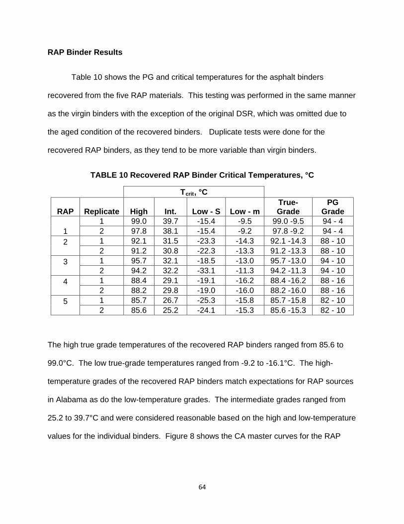
RAP Binder Results
Table 10 shows the PG and critical temperatures for the asphalt binders
recovered from the five RAP materials. This testing was performed in the same manner
as the virgin binders with the exception of the original DSR, which was omitted due to
the aged condition of the recovered binders. Duplicate tests were done for the
recovered RAP binders, as they tend to be more variable than virgin binders.
TABLE 10 Recovered RAP Binder Critical Temperatures, °C
Tcrit, °C
RAP Replicate High Int. Low - S Low - m
True- Grade
PG Grade
1 1 99.0 39.7 -15.4 -9.5 99.0 -9.5 94 - 4 2 97.8 38.1 -15.4 -9.2 97.8 -9.2 94 - 4
2
1 92.1 31.5 -23.3 -14.3 92.1 -14.3 88 - 10 2 91.2 30.8 -22.3 -13.3 91.2 -13.3 88 - 10
3
1 95.7 32.1 -18.5 -13.0 95.7 -13.0 94 - 10 2 94.2 32.2 -33.1 -11.3 94.2 -11.3 94 - 10
4
1 88.4 29.1 -19.1 -16.2 88.4 -16.2 88 - 16 2 88.2 29.8 -19.0 -16.0 88.2 -16.0 88 - 16
5
1 85.7 26.7 -25.3 -15.8 85.7 -15.8 82 - 10 2 85.6 25.2 -24.1 -15.3 85.6 -15.3 82 - 10
The high true grade temperatures of the recovered RAP binders ranged from 85.6 to
99.0°C. The low true-grade temperatures ranged from -9.2 to -16.1°C. The high-
temperature grades of the recovered RAP binders match expectations for RAP sources
in Alabama as do the low-temperature grades. The intermediate grades ranged from
25.2 to 39.7°C and were considered reasonable based on the high and low-temperature
values for the individual binders. Figure 8 shows the CA master curves for the RAP
64

binders. Figure 9 shows a summary of the master curves for all seven binders that
were tested as part of this study.
Figure 8 Recovered Binder Master Curves @ 25°C
1.E-01
1.E+00
1.E+01
1.E+02
1.E+03
1.E+04
1.E+05
1.E+06
1.E-06 1.E-04 1.E-02 1.E+00 1.E+02 1.E+04 1.E+06
G* b
inde
r, kP
a
Log Reduced Frequency, Hz
RAP 1 RAP 2 RAP 3 RAP 4 RAP 5
65

Figure 9 Master Curves for all Binders @ 25°C
As expected based on the PG grades, the RAP binder master curves are stiffer than the
virgin binder master curves. RAP 1 is the stiffest binder at high-temperatures while
RAP 5 is the least stiff. As the temperature decreases, the differences between the
stiffnesses of the seven binders are reduced. This can be seen in the master curves,
with RAP 1 and RAP 5 converging as frequency increases. RAP 2, RAP 3, and RAP 4
are very similar in their stiffness properties, which again is reflected in the master
curves.
TORSION BAR STIFFNESS TEST RESULTS
In this chapter, the results obtained from torsion bar testing of the virgin and
100% RAP materials are presented and analyzed. The goal of this portion of the study
was to determine if the torsion bar procedure produced mixture stiffness data of suitable
1.E-03
1.E-02
1.E-01
1.E+00
1.E+01
1.E+02
1.E+03
1.E+04
1.E+05
1.E+06
1.E-06 1.E-04 1.E-02 1.E+00 1.E+02 1.E+04 1.E+06
G* b
inde
r, kP
a
Log Reduced Frequency, Hz
PG 64-22 PG 76-22 RAP 1 RAP 2
RAP 3 RAP 4 RAP 5
66

quality. The factors considered included repeatability, data trends, and suitability for
creating the master curves needed for backcalculation.
Virgin Torsion Bars
For ease of reference in this and later sections, the torsion bar specimens made
with aggregate that was split over the #4 sieve will be referred to as -4 while the
specimens made with aggregate that was split over the #8 sieve will be referred to as
-8. Figures 10 and 11 show the G*mix and δmix results at 20°C for the virgin binders.
The results shown are the average of four replicate test specimens. Error bars showing
the standard deviation of the test results are included to show the variability within each
set of replicate tests.
Figure 10 Virgin Torsion G*mix Results @ 20°C
-
500
1,000
1,500
2,000
2,500
3,000
3,500
0.01 0.02 0.05 0.10 0.22 0.46 1.00 2.15 4.64 10.00
G* m
ix, M
Pa
Frequency, Hz
PG 64-22 -4 PG 64-22 -8 PG 76-22 -4 PG 76-22 -8
67

Figure 11 Virgin Torsion δmix Results @ 20°C
Trends for G*mix and δmix at the other test temperatures were similar to the
results shown. Complete torsion bar results for these mixes can be found in Appendix
C.
The torsion bar results for the virgin materials followed the expected trends for
mixture stiffness testing using other test methods. The G*mix values increase with
increasing frequency and decrease with increasing temperature. The change in
stiffness with increasing frequency as more pronounced at lower temperatures, with an
almost 500% increase in G*mix between the 0.01 and 10 Hz frequencies at 20°C. At
60°C, the G*mix values are significantly lower at all frequencies and do not increase as
much from 0.01 to 10 Hz. At warmer temperatures and frequencies where the binder is
0
5
10
15
20
25
30
35
40
45
0.01 0.02 0.05 0.10 0.22 0.46 1.00 2.15 4.64 10.00
δ mix, d
egre
es
Frequency, HzPG 64-22 -4 PG 64-22 -8 PG 76-22 -4 PG 76-22 -8
68

softer, the aggregate structure begins to play more of a role in the stiffness properties of
the mixture, and differences in binder stiffness may become less pronounced.
For both virgin binders, the -8 G*mix values were higher than the -4 G*mix values.
Of the four datasets, the PG 76-22 test specimens made with -8 aggregate had the
highest G*mix values. The PG 76-22 test specimens made with -4 aggregate had much
lower G*mix values than the -8 specimens, and in some cases were less stiff than the
PG 64-22 test specimens made with -4 aggregate. The PG 64-22 virgin binder test
specimens made with both the -4 and -8 aggregate generally had lower G*mix than the
PG 76-22 test specimens, although in a few instances they were slightly higher than the
PG 76-22 -4 values.
The δmix results for the virgin torsion bars also matched expected behavior for
asphalt mixture testing. The δmix values decrease with increasing frequency for the
20°C tests. This is typical behavior seen in asphalt binder testing (phase angle
decreases as the binder stiffness increases, indicating that the binder is approaching an
elastic state) and is expected given the increased role of the asphalt binder in the mix at
the colder temperatures. The δmix appear to plateau and change very little with
increasing frequency at 30°C. At 40°C and above, the δmix plateau at the lower
frequencies, then increase with increasing frequency, indicating the increased role of
the aggregate as the asphalt binder softens at high-temperatures.
Differences in δmix between the datasets are less pronounced than the
differences in G*mix. Mix tests tend to be less sensitive to phase angle than binder
tests. The PG 76-22 test specimens made with -8 aggregate had the lowest δmix, which
69

was expected given that this dataset had the highest G*mix and also because the PG
76-22 is a polymer modified binder. Both of these conditions lead to reduced phase
angles. The PG 76-22 made with the -4 aggregate did not follow the expected trends at
lower temperatures and had δmix that were higher than the PG 64-22 datasets. At 50
and 60°C, the PG 76-22 made with -4 aggregates had δmix values that were lower than
the PG 64-22 datasets, better matching expected behavior. The PG 64-22 -4 and -8
datasets had δmix values that were typically higher than the PG 76-22 test results. For
the PG 64-22 test specimens, the different aggregate sizes didn’t show large
differences in δmix. Overall, the δmix values for the virgin binder tests had a very limited
range. Most δmix values, regardless of testing conditions, fell between 20 and 35°.
Figures 12 and 13 show the coefficient of variation (COV) values at 10Hz for both
G*mix and δmix.
70

Figure 12 COV at 10Hz for all Test Temperatures – Virgin Binder Torsion Bars G*mix
Figure 13 COV at 10Hz for all Test Temperatures – Virgin Binder Torsion Bars δmix
0%
5%
10%
15%
20%
25%
20 30 40 50 60
CO
V
Temperature, °C
PG 64-22 -4 PG 64-22 -8 PG 76-22 -4 PG 76-22 -8
0%
5%
10%
15%
20%
25%
20 30 40 50 60
CO
V
Temperature, °CPG 64-22 -4 PG 64-22 -8 PG 76-22 -4 PG 76-22-8
71

At the time the testing was conducted, there was no official recommendation for
acceptable variability between replicate samples. However, the ASTM D7552-09 test
method, published after testing was completed, requires that COV values for replicate
data at the 10Hz frequency level for all temperatures be less than 15%. As can be seen
from Figure 12, a few of the test results at high-temperature/low frequency conditions
had COV values above 20% but were in all cases less than 25% and in most cases met
the 15% requirement. There also appears to be a trend of increasing COV with
increasing temperature (for all but the PG 76-22 -8 specimens). The softer PG 64-22
torsion bar specimens have higher COV than the stiffer PG 76-22 specimens. Although
ASTM D7552 does not recommend a COV level for δmix, it can be seen from Figure 13
that the δmix results at 10Hz are all below 15% COV, with the exception of the PG 64-22
results at 60°C. Again, there appears to be less variability in the data at the colder
temperatures.
The quality of the data for creating master curves was evaluated using Black
Space diagrams. Plots of δmix verses the log (G*mix) were plotted for the average
results at all temperatures and a polynomial trend-line fitted to the data. The
smoothness of the data points indicates whether the data is of acceptable quality.
Typically values of R2 less than 0.90 are rejected (30). Figures 14 and 15 show the
Black Space diagrams for the virgin binder torsion bar results. The data shown is an
average of the 4 replicates for each material.
72

Figure 14 Black Space Diagram for PG 64-22 Virgin Torsion Results
Figure 15: Black Space Diagram for PG 76-22 Virgin Torsion Results
R² = 0.7611
R² = 0.904
7
12
17
22
27
32
37
6 6.5 7 7.5 8 8.5 9 9.5 10
δ mix, d
egre
es
Log G*mix, PaPG 64-22 -4 PG 64-22 -8
R² = 0.9535
R² = 0.91
7
12
17
22
27
32
37
6 6.5 7 7.5 8 8.5 9 9.5 10
δ mix, d
egre
es
Log G*mix, Pa PG 76-22 -4 PG 76-22 -8
73

For the PG 64-22 materials, the R2 value for the -4 mix did not meet the smoothness
requirement. The PG 64-22 -8 mix did have an acceptable R2 (0.92). The low R2 for
the PG 64-22 -4 mixes may be due to increased variability in the lower frequencies of
the 50 and 60°C data (and removal of these data sets would have improved the R2
value for this mix to 0.90, although no data was actually removed from the analysis at
this time). Both sets of PG 76-22 virgin mixes had adequate R2 values. Overall,
excepting a few issues with the high-temperature tests, the DSR torsion bar tests on the
virgin mixes provided reasonable results that could be used to create master curves.
For the mixture tests, master curves were created using the generalized logistic
equation shown in Equation 16. Figure 16 shows a comparison of the four sets of virgin
torsion bar master curves while Figure 17 shows a comparison of the torsion bar and
binder master curves. Again, the results shown are the average values for four
replicates.
74

Figure 16 Virgin Torsion Bar Master Curve – PG 64-22 -4
Figure 17 Virgin G*mix and G*binder Master Curves @ 25°C
1.E+03
1.E+04
1.E+05
1.E+06
1.E+07
1.E+08
1.E+09
1.E-06 1.E-04 1.E-02 1.E+00 1.E+02 1.E+04
G* b
inde
r, kP
a
Log Reduced Frequency, Hz
PG 64-22 -4 PG 64-22 -8 PG 76-22 -4 PG 76-22 -8
1.E-03
1.E-01
1.E+01
1.E+03
1.E+05
1.E+07
1.E+09
1.E-06 1.E-04 1.E-02 1.E+00 1.E+02 1.E+04 1.E+06
G* b
inde
r, kP
a
Log Reduced Frequency, HzPG 64-22 -4 PG 64-22 -8 PG 76-22 -4PG 76-22 -8 PG 64-22 Binder PG 76-22 Binder
75

The master curves show that, as expected, the torsion bar stiffness results were
stiffer than the binder stiffness values. For the torsion bars, the PG 76-22 -8 specimens
appear to be the stiffest at lower frequencies while the other three mixtures have similar
stiffnesses. At the higher frequencies, the PG 76-22 -4 specimens are the least stiff
while the other combinations have similar stiffness values. Based on these results, it
does not appear that there is a great difference in stiffness values between the binders
or aggregates except at the extremes of high or low stiffness.
Statistical analyses were performed on the virgin torsion bar results to compare
the effects of aggregate size and binder type on the G*mix values. The aggregate size
comparison was made to determine if the different aggregate sizes affected the mixture
stiffness results. The binder type comparison was to determine if the torsion bar test is
sensitive enough to identify differences in mixture stiffness due to different binder types.
Table 11 shows the summary of a two-sample statistical t-test analysis (α = 0.05) on
aggregate size for both virgin binders (H0: x̄ -4 = x̄ -8). A separate analysis was
performed at each test temperature and frequency (0.1, 1.0, and 10.0 Hz) to see if
aggregate size caused a significant difference in the G*mix values measured by the test
results.
76

TABLE 11 t-test Analysis for Aggregate Size – p-values
Average G*mix, kPa
PG 64-22 PG 76-22
Freq. Temp,
°C -4 -8 p-value -4 -8 p-value
0.1Hz
20 606,000 661,725 0.288 659,200 1,042,000 0.000 30 252,700 257,525 0.895 268,150 468,300 0.000 40 110,498 131,410 0.253 123,550 245,600 0.000 50 67,543 87,930 0.137 73,128 154,025 0.000 60 40,833 62,115 0.051 50,105 106,075 0.000
1 Hz
20 1,235,250 1,324,250 0.251 1,335,500 1,822,750 0.000 30 500,150 512,125 0.796 540,275 834,900 0.000 40 218,475 228,400 0.634 220,150 400,025 0.000 50 110,950 136,700 0.113 114,488 227,925 0.000 60 59,590 85,828 0.006 68,358 141,450 0.000
10Hz
20 2,315,250 2,477,750 0.330 2,494,250 3,027,000 0.003 30 1,050,150 1,090,500 0.543 1,134,250 1,531,250 0.000 40 491,950 474,975 0.985 459,625 729,400 0.000 50 225,850 261,375 0.346 219,175 389,725 0.000 60 109,145 143,475 0.082 112,085 215,775 0.000
The p-values shown in Table 11 represent the probability of getting similar results
if the null hypothesis, H0, is true. The farther away the test statistic from the t-test is
located on the tails of the standard normal distribution, the smaller the p-value will be.
For the chosen significance level of 0.05, a p-value of greater than 0.05 will result in a
failure to reject the null hypothesis. P-values less than 0.05 indicate that the results are
too far apart and therefore the null hypothesis must be rejected. Based on the
statistical analysis the PG 64-22 -4 G*mix results were statistically the same as the -8
G*mix results for 14 out of the 15 cases (failed to reject H0: x̄ -4 = x̄ -8 ). The PG 76-22
G*mix results for the two aggregate sizes were statistically different in all cases. These
77

results indicate that aggregate structure may have an influence on the results of the
torsion bar tests.
A similar statistical analysis was done comparing the G*mix results across binder
type to determine if the torsion bar test was sensitive enough to distinguish between the
two virgin binders (H0: x̄ 64 = x̄ 76) . Table 12 shows the p-values for comparisons of the
PG 64-22 and PG 76-22 mixes including comparisons of both aggregate sizes and
when separated into -4 and -8 aggregate. Again, cells with p-values less than 0.05
indicate a statistically significant difference (rejection of H0) between the PG 64-22 and
PG 76-22 tests.
78

TABLE 12 t-test Analysis for Binder Type – p-value
Average G*mix, kPa
All -4 -8
Freq, Hz
Temp, °C PG 64-22 PG 76-22
p-value PG 64-22 PG 76-22
p-value PG 64-22 PG 76-22
p-value
0.1
20 633,863 850,600 0.025 606,000 659,200 0.357 661,725 1,042,000 0.000 30 255,113 368,225 0.051 252,700 268,150 0.655 257,525 468,300 0.001 40 120,954 184,575 0.031 110,498 123,550 0.966 131,410 245,600 0.003 50 77,736 113,576 0.008 67,543 73,128 0.566 87,930 154,025 0.003 60 51,474 78,090 0.004 40,833 50,105 0.241 62,115 106,075 0.003
1
20 1,279,750 1,579,125 0.020 1,235,250 1,335,500 0.207 1,324,250 1,822,750 0.000 30 506,138 687,588 0.018 500,150 540,275 0.388 512,125 834,900 0.000 40 223,438 310,088 0.049 218,475 220,150 0.826 228,400 400,025 0.001 50 123,825 171,206 0.079 110,950 114,488 0.715 136,700 227,925 0.002 60 72,709 104,904 0.069 59,590 68,358 0.249 85,828 141,450 0.002
10
20 2,396,500 2,760,625 0.020 2,315,250 2,494,250 0.209 2,477,750 3,027,000 0.017 30 1,070,325 1,332,750 0.012 1,050,150 1,134,250 0.204 1,090,500 1,531,250 0.001 40 483,463 594,513 0.064 491,950 459,625 0.722 474,975 729,400 0.003 50 243,613 304,450 0.133 225,850 219,175 0.758 261,375 389,725 0.027 60 126,310 163,930 0.123 109,145 112,085 0.757 143,475 215,775 0.021
79

The statistical analysis showed that the G*mix results could distinguish between the
different binder types at 9 out of the 15 temperatures and frequencies shown when the
two aggregate sizes were combined and analyzed together. When analyzing the two
aggregate sizes separately, the -8 aggregate test specimens could distinguish between
binder type in all cases while the -4 aggregate size could not.
Based on the quality of the data shown, the torsion bar test was considered to be
an adequate candidate for further testing. The G*mix and δmix results measured by the
test were reasonable in behavior and repeatability and seemed to be of adequate
quality for the creation of master curves. The lack of ability to distinguish between the
two virgin binders for one aggregate size was a concern, but since two out of the three
comparisons (all aggregate and -8 aggregates) did show statistically significant
differences in G*mix, it was decided to continue testing for the 100% RAP mixes.
RAP Torsion Bars
Figures 18 and 19 show the G*mix and δmix results for the torsion bar samples
made using the five RAP materials at 20°C. Due to time and material restrictions, it was
decided to use only the -4 aggregate size for the RAP specimens. This size was
chosen due to some testing issues that occurred with the -8 virgin specimens (high rate
of sample breakage and difficulty getting consistent air voids) and also because this
seems to be the most commonly used size for separating coarse and fine RAP
materials and allowed for direct sampling at the mix plant if necessary. The results
shown are the average of four replicate test specimens. Complete torsion bar results
for the RAP samples can be found in Appendix C.
80

Figure 18 RAP Torsion G*mix Results @ 20°C
Figure 19 RAP Torsion δmix Results @ 20°C
The torsion bar test results for the RAP materials followed the same trends as
the virgin torsion bar tests. The G*mix values increased with increasing frequency and
decreased with increasing temperature. Differences in stiffness between RAPs are
-
1,000
2,000
3,000
4,000
5,000
6,000
0.01 0.02 0.05 0.10 0.22 0.46 1.00 2.15 4.64 10.00
G* m
ix, M
Pa
Frequency, HzRAP 1 RAP 2 RAP 3 RAP 4 RAP 5
0
5
10
15
20
25
30
35
0.01 0.02 0.05 0.10 0.22 0.46 1.00 2.15 4.64 10.00
δ mix, d
egre
es
Frequency, HzRAP 1 RAP 2 RAP 3 rAP 4 RAP 5
81

more apparent at colder temperatures where the asphalt binder influence on stiffness is
strongest. As the test temperature increased and test frequency decreased, the
differences in G*mix values decreased. RAPs 1 and 5 had higher G*mix values at all
temperatures and frequencies than the other RAP sources. RAPs 2, 3, and 4 all had
much lower G*mix values. RAP 3 appears to have less sensitivity to changes in
temperature or frequency than the other RAPs, and therefore had higher G*mix than
RAPs 2 and 4 as the test temperature increases.
The δmix decreased with increasing frequency at the lower temperature,
appeared to plateau around 50°C, and then decreased with increasing frequency.
Figures 20 and 21 show the COV values for the RAP specimens at 10Hz. RAPs 1 and
5 had the lowest overall δmix compared to the other RAP sources, followed by RAP 3.
RAPs 2 and 4 had the highest δmix.
82

Figure 20 COV at 10Hz for all Test Temperatures – RAP Torsion Bars G*mix
Figure 21 COV at 10Hz for all Test Temperatures – RAP Torsion Bars δmix
0%
5%
10%
15%
20%
25%
20 30 40 50 60
CO
V
Temp, °CRAP 1 RAP 2 RAP 3 RAP 4 RAP 5
0%
5%
10%
15%
20%
25%
30%
35%
20 30 40 50 60
CO
V
Temp, °C
RAP 1 RAP 2 RAP 3 RAP 4 RAP 5
83

Like the virgin binder torsion bars, the RAP torsion bar specimens for the most part had
acceptable COV values. RAP 2 had COV values for G*mix that were slightly higher than
the 15% limit. RAP 5 had G*mix and δmix COV that were high at 20°C. The trend of
increasing COV with decreasing binder stiffness as seen in the specimens with virgin
binders was not apparent with the RAP specimens. This may be due to the higher
stiffness of the RAP binders at the test temperatures that reduced the influence of the
aggregate structure.
When used to make Black Space diagrams, all the RAP torsion results had R2
values greater than 0.90. This indicates that the G*mix results from the torsion bar tests
on RAP specimens provided data that was of acceptable quality for the creation of
master curves. Figure 22 shows the master curves created from the RAP torsion bar
G*mix results. Figure 23 shows the RAP G*mix master curves compared to the master
curves created from the G*binder frequency sweeps on the recovered RAP binders. The
values shown are averages of 4 replicate test specimens for each RAP source.
84

Figure 22 RAP Torsion Bar Master Curves @ 25°C
Figure 23 Comparison of RAP Binder and Torsion Bar Master Curves @ 25°C
1.E+03
1.E+04
1.E+05
1.E+06
1.E+07
1.E+08
1.E-05 1.E-03 1.E-01 1.E+01 1.E+03
G* m
ix. k
Pa
Log Reduced Frequency, Hz
RAP 1 Torsion RAP 2 Torsion RAP 3 TorsionRAP 4 Torsion RAP 5 Torsion
1.E+00
1.E+01
1.E+02
1.E+03
1.E+04
1.E+05
1.E+06
1.E+07
1.E+08
1.E-05 1.E-03 1.E-01 1.E+01 1.E+03
G* m
ix. k
Pa
Log Reduced Frequency, Hz
RAP 1 Torsion RAP 2 Torsion RAP 3 Torsion RAP 4 TorsionRAP 5 Torsion RAP 1 Binder RAP 2 Binder RAP 3 BinderRAP 4 Binder RAP 5 Binder
85

The G*mix master curves ranked the RAP sources slightly differently than the G*binder
master curves. For the binders, RAP 1 was the stiffest material while RAP 5 was the
softest. RAP 2 and RAP 4 were very similar according to the binder master curves.
RAP 3 was the second stiffest after RAP 1. For the mixes, RAPs 1 and 5 appeared to
have very similar stiffness values while RAP 2 was the least stiff at high-temperature,
low frequencies. RAPs 3 and 4 were similar at the high-temperature, low stiffness
region, but diverged as stiffness increased. There are several possible reasons for
these differences, mainly the effect of aggregates and air voids on the stiffness
properties of the mixture test specimens. There may also be some differences in
binder properties between the recovered RAP binders that have been through the
extraction/recovery process and the actual RAP binder in the RAP mixtures.
A statistical general linear model Analysis of Variance (ANOVA) test was
performed on the 100% RAP G*mix results to determine if there was any statistical
difference between the RAP stiffness values for the different RAP sources (H0: x̄ 1
=
x̄ 2 = x̄ 3 = x̄ 4 = x̄ 5). In the cases where there were statistical differences found, Tukey-
Kramer comparisons (α = 0.05) were performed on the replicate data for the RAP
torsion bars to determine which of the datasets differed from the others. The analysis
was done for each temperature and at three frequencies (0.1, 1.0, and 10.0 Hz). The
results of the ANOVA analysis are summarized in Table 13. For each row in the table,
RAP sources with the same letter indicate that the average G*mix values were found to
be statistically the same. RAP sources with different letters were found to be
statistically different. RAP sources with two letters had average G*mix values that were
86

statistically the same as two other RAP sources that were not statistically the same. For
example, at 50°C and 0.1Hz, the statistical analysis found the average G*mix values for
RAPs 1 and 5 to be statistically the same. The average G*mix values for RAP 5 were
also statistically the same as for RAP 3, although RAP 3 was not a statistical match for
RAP 1. The average G*mix values for RAPs 2 and 4 were statistically the same as
each other and different from RAPs 1, 3, and 5.
TABLE 13 ANOVA Analysis of RAP Source
RAP
Freq Temp,
°C 1 2 3 4 5
0.1Hz
20 A B B B AB 30 A B B B A 40 A C B BC A 50 A C B C AB 60 B C B C A
1 Hz
20 A A A A A 30 A B B B A 40 A B B B A 50 A C B C A 60 A B A B A
10Hz
20 AB AB B AB A 30 AB C C BC A 40 A B B B A 50 A B B B A 60 A C B C A
Per the statistical analysis, the average G*mix values for RAPs 1 and 5 were
statistically the same in most cases. The average G*mix values for RAPs 2, 3, and 4
were also statistically the same at lower temperatures, while differing at higher
temperatures. When the virgin binder torsion bar results were compared to the torsion
bar results using a similar analysis, the Tukey groupings placed them in a separate
87

group from the RAP torsion bar results in all cases. This indicated that the torsion bar
results could distinguish between the virgin mix specimens and the much stiffer RAP
specimens.
Summary
The following observations were made at the conclusion of the torsion bar
mixture stiffness testing:
1. The mixture stiffness data obtained from the torsion bar tests resembled that of
other mixture stiffness tests in both behavior and quality.
2. The mixture stiffness data obtained for both the virgin binders and 100% RAP
test specimens met the data quality requirements for the construction of master
curves according to the use of Black Space diagrams. The only exception was
the PG 64-22 binder which had issues with testing variability at the high-
temperature and low-frequency test parameters. It appears from this dataset that
the torsion bar procedure may not be suited for mixtures with very low stiffness
values. The stiffer PG 76-22 and 100% RAP mixes did not have the same
problem, nor did the PG 64-22 mixes at lower temperatures or higher
frequencies.
3. While the backcalculated torsion bar G*mix values could not distinguish between
the two virgin binders at one of the aggregate sizes, they could distinguish
between the 100% RAP sources in several instances. The torsion bar G*mix
values were also able to group the results of the virgin binder specimens as
being statistically different than the 100% RAP specimens. It was unclear how
88

much influence the effects of aggregate structure and air voids have on the
mixture stiffness values, but analysis of the -4 and -8 aggregate sizes for the
virgin binders indicates that aggregate structure may be an important factor. This
was also indicated by the different rankings of the RAP torsion bar results and
the recovered RAP binder results.
4. Even though it was unclear how well the mixture stiffness results could
distinguish between the materials in the torsion specimens, the ultimate goal of
this research was the estimation of the properties of the asphalt binder in the
mixes. The Hirsch model chosen for this calculation takes the volumetric factors
into account; therefore the estimated binder properties may not be as affected by
the aggregate structure as the mixture stiffness values.
BACKCALCULATION RESULTS
Once a complete set of mixture stiffness data had been obtained for the virgin
and 100% RAP test specimens, the next step in the study evaluated the ability of the
Hirsch model to accurately predict G*binder. The first evaluation performed was to
determine the effectiveness of the Hirsch model as written for calculating G*mix based
on tested G*binder. Theoretically, if the model can accurately forward-calculate G*mix, it
should also be able to backcalculate G*binder. It was expected that the model would
need to be adjusted to improve its accuracy as the original version of the model was
calibrated for a different test procedure. Once a revised version of the model was
developed to forward-calculate G*mix, both versions of the formula were used to
backcalculate a set of binder test results.
89

Evaluation of Hirsch Model for High and Intermediate-temperatures
In theory, if the Hirsch model can accurately estimate the G*mix based on tested
G*binder, then the model might also be capable of estimating G*binder based on tested
G*mix values. The Hirsch model for G* is shown in Equations 7 and 8 and is repeated
below.
( )
∗+
−−
+
∗+
−=
binder
VMAc
bindercmix
GVFAVMA
PVFAVMAGVMAPG
*000,6011
1000,10
*100
1000,601*100
(7)
Where: VMA = voids in mineral Aggregate, %;
VFA = voids Filled with asphalt, %;
G*binder = binder complex shear modulus, psi;
Pc = contact factor, obtained from Equation 8; and
G*mix = mix complex shear modulus, psi – obtained from torsion bar test.
678.0*396
678.0*3
∗+
∗+
=
VMAbinder
GVFA
VMAbinder
GVFA
cP (8)
The G* version of the Hirsch model was chosen for this project because the torsion bar
test method results in a measurement of complex shear modulus. The torsional
sinusoidal loading used in the torsion bar procedure also more closely matched the
90

loading used in the SST Frequency Sweep at Constant Height test used to measure
G*mix than it does the compressive loading used to measure E*mix. The original version
of the model was not expected to be an exact fit for the torsion bar data G*mix results
since it was calibrated for a much larger sample and a straight shear load instead of the
small torsion bars subjected to a torsional twisting load. As such, the first step in
evaluating the effectiveness of the model was to use the DSR data obtained from the
RTFO-aged virgin binder frequency sweeps to calculate values of G*mix. The VMA and
VFA values measured by the dimensional analysis of the individual torsion specimens
were used to calculate replicate test results. The calculated G*mix values were then
compared to the individual G*mix values measured in the previous section. The results of
the comparison were used to verify the accuracy of the model shown in Equations 7 and
8 for estimating G*mix for the torsion bars. Figures 24 and 25 show the comparison of
calculated and tested G*mix values using the original Hirsch G*mix model for the virgin
materials. The data in these figures includes the entire set of test results for both the -4
and -8 aggregate sizes. Linear regression was performed to determine the line of best
fit for the data, along with 95% confidence intervals for the results.
91

Figure 24 Comparison of Calculated vs. Tested G*mix for Virgin PG 64-22 – Original Model
Figure 25 Comparison of Calculated vs. Tested G*mix for Virgin PG 76-22 – Original Model
R² = 0.9734
0.0E+00
5.0E+02
1.0E+03
1.5E+03
2.0E+03
2.5E+03
3.0E+03
0.0E+00 5.0E+02 1.0E+03 1.5E+03 2.0E+03 2.5E+03 3.0E+03
Cal
cula
ted
G* m
ix, M
Pa
Tested G*mix, MPaLine of Equality 95% CI Linear Reg
R² = 0.9352
0.0E+00
5.0E+02
1.0E+03
1.5E+03
2.0E+03
2.5E+03
3.0E+03
3.5E+03
0.0E+00 5.0E+02 1.0E+03 1.5E+03 2.0E+03 2.5E+03 3.0E+03 3.5E+03
Cal
cula
ted
G* m
ix, M
Pa
Tested G*mix, MPa
Line of Equality 95% CI Linear Reg
92

The 95% confidence interval for the data was calculated using equation 18 as follows:
𝐶𝐼 = �̅� ± 𝑡𝑛−1 �𝑠√𝑛� (18)
Where:
�̅� = sample mean;
tn-1 = t-value representing n-1 degrees of freedom, 0.05 confidence level;
n= sample size;
s = sample standard deviation.
A confidence interval expresses the degree of uncertainty about the linear regression. If
the formula generated by the linear regression line is used to calculate G*mix based on a
tested G*mix value, the result will lie within this interval 95% of the time. The width of a
confidence interval gives an indication of how uncertain the data is. The wider the
interval, the more uncertain the data.
As seen in the figures, the original version of the Hirsch model almost always
under-estimated G*mix when compared to actual tested data from the torsion bars. A
paired -sample t-test (α = 0.05) analysis comparing the difference between the
individual pairs of tested and calculated data showed the tested results were statistically
larger than the calculated G*mix values and confirmed that the calculated results were
statistically different from the line of equality.
To improve the accuracy of the calculated G*mix results, a calibration of the
model was performed. In order to complete this task, the calculated G*mix values for the
virgin materials were compared to the tested G*mix values and a non-linear least
93
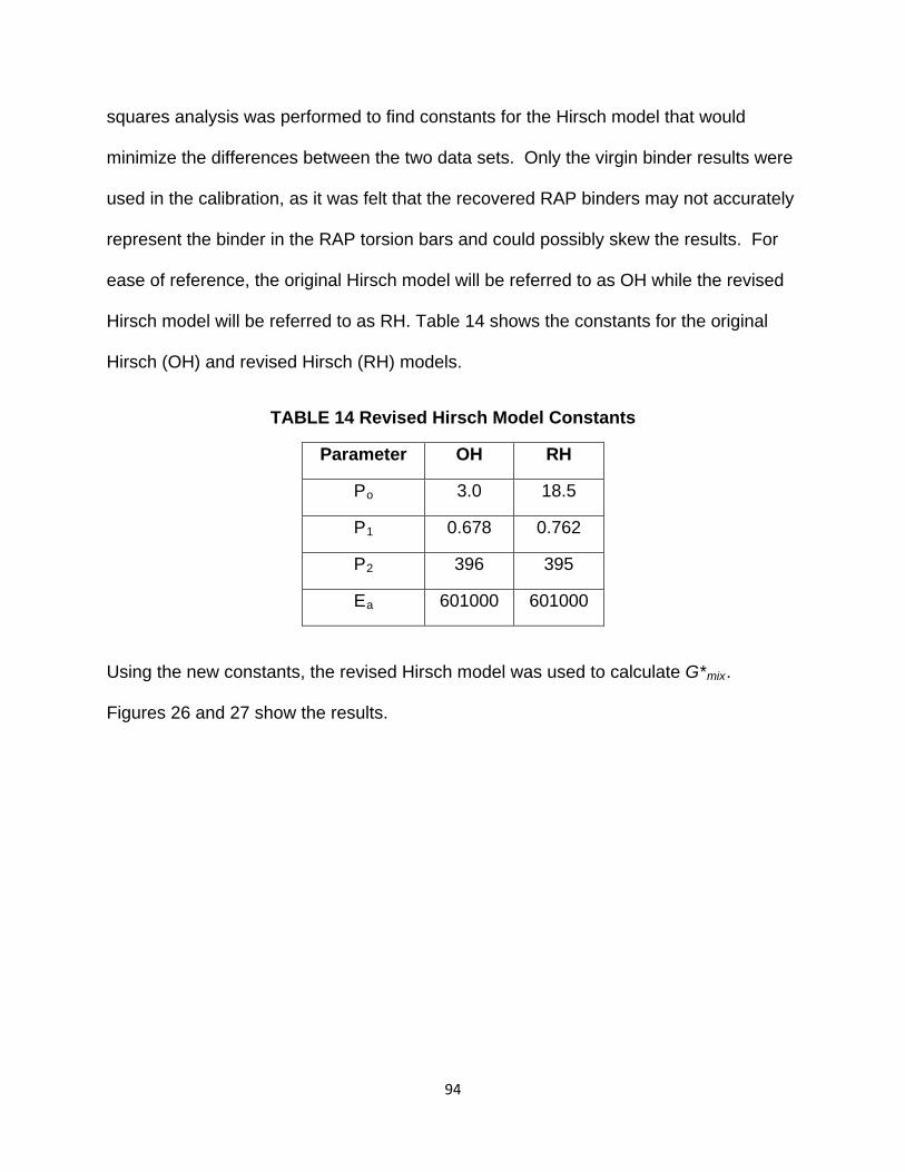
squares analysis was performed to find constants for the Hirsch model that would
minimize the differences between the two data sets. Only the virgin binder results were
used in the calibration, as it was felt that the recovered RAP binders may not accurately
represent the binder in the RAP torsion bars and could possibly skew the results. For
ease of reference, the original Hirsch model will be referred to as OH while the revised
Hirsch model will be referred to as RH. Table 14 shows the constants for the original
Hirsch (OH) and revised Hirsch (RH) models.
TABLE 14 Revised Hirsch Model Constants
Parameter OH RH
Po 3.0 18.5
P1 0.678 0.762
P2 396 395
Ea 601000 601000
Using the new constants, the revised Hirsch model was used to calculate G*mix.
Figures 26 and 27 show the results.
94

Figure 26 Comparison of Calculated vs. Tested G*mix for Virgin PG 64-22 – Revised Model
Figure 27 Comparison of Calculated vs. Tested G*mix for Virgin PG 76 - 22 – Revised Model
R² = 0.9677
0.0E+00
5.0E+02
1.0E+03
1.5E+03
2.0E+03
2.5E+03
3.0E+03
3.5E+03
0.0E+00 5.0E+02 1.0E+03 1.5E+03 2.0E+03 2.5E+03 3.0E+03 3.5E+03
Cal
cula
ted
G* m
ix, M
Pa
Tested G*mix, MPa
Line of Equality 95% CI Linear Reg
R² = 0.9223
0.0E+00
5.0E+02
1.0E+03
1.5E+03
2.0E+03
2.5E+03
3.0E+03
3.5E+03
0.0E+00 5.0E+02 1.0E+03 1.5E+03 2.0E+03 2.5E+03 3.0E+03 3.5E+03
Cal
cula
ted
G* m
ix, M
Pa
Tested G*mix, PaLine of Equality 95% CI Linear Reg
95

For the revised version of the Hirsch model, a paired-sample t-test analysis (α = 0.05)
indicated that the calculated and tested G*mix values were still not statistically equal.
Visually, however, the revised version of the Hirsch model resulted in an improved
estimation of G*mix obtained from the virgin torsion bar samples.
Once it was determined that the revised Hirsch model gave an improved
estimate of the virgin binder torsion bar properties, it was used to calculate the G*mix
values for the 100% RAP torsion bar specimens using the DSR data from the recovered
RAP binders. Figure 28 shows a comparison of the actual and calculated G*mix using
both the original and revised Hirsch model coefficients for the five RAP samples used in
the study.
96

Figure 28 Comparison of Calculated vs. Tested G*mix for RAP Torsion Samples
Figure 28 shows a similar trend for the RAP materials as for the virgin materials. The
original Hirsch model formula underestimated the calculated G*mix values. The revised
Hirsch model, while not improving the RAP results as much as the virgin results, does
bring the results closer to the line of equality. A paired-sample t-test (α = 0.05) analysis
comparing the calculated and tested G*mix values that the two sets of data (original and
revised Hirsch) are statistically different, both from each other and from the line of
equality. Figure 29 shows the comparison results for RAP 1. Plots of the comparison
for the other RAP sources can be found in Appendix D.
R² = 0.8900
R² = 0.8770
0.0E+00
1.0E+03
2.0E+03
3.0E+03
4.0E+03
5.0E+03
0.0E+00 1.0E+03 2.0E+03 3.0E+03 4.0E+03 5.0E+03
Cal
cula
ted
G* m
ix, M
Pa
Tested G*mix, MPa
Original Model Revised Model Line of Equality 95% CI Orig 95% CI Rev
97

Figure 29 RAP 1 Calculation Comparison for Original and Revised Hirsch
The figure shows that, even though the revised Hirsch model provides improved
correlation between the tested and calculated G*mix values for the RAP materials, the
improvement is not quite as good as for the virgin materials. For RAPs 2 and 5, the
improvement was only slight, while RAPs 1, 3, and 4 showed better agreement between
calculated and tested G*mix. This is not necessarily the fault of the calculation and may
be due to the inability to adequately characterize RAP binders using extracted and
recovered binder. Figure 29 also shows what appears to be a plateau in the G*mix
results at higher stiffness values (high frequency, cold temperature region). This
plateau behavior was seen in all the RAP G*mix plots and to a lesser extent in Figures
24 – 27. Christensen et al. noted the tendency of the G*mix values calculated using the
Hirsch model to plateau in this region and attributed it to the use of the estimated
constant aggregate modulus value (601,000 psi for the original Hirsch model) in the
R² = 0.9511
R² = 0.9208
0.0E+00
5.0E+02
1.0E+03
1.5E+03
2.0E+03
2.5E+03
3.0E+03
3.5E+03
4.0E+03
0.0E+00 5.0E+02 1.0E+03 1.5E+03 2.0E+03 2.5E+03 3.0E+03 3.5E+03 4.0E+03
Cal
cula
ted
G* m
ix, M
Pa
Tested G*mix, MPaOriginal Model Revised Model Line of Equality 95% CI Orig 95% CI Rev
98

calculation. This value acts as a limiting value for the asphalt mixture stiffness
calculated using the model. This behavior was not believed to be of any concern, as
the range of stiffness values at which it occurs is much higher than any the asphalt
mixture would experience in a pavement (27).
Based on the forward calculation results, it was felt that the revised Hirsch model
might be able to provide an improved estimate of backcalculated G*binder results. In the
following section, both the original and revised forms of the model were used for
backcalculation so that the final results could be compared to further study the accuracy
of the revised model.
Virgin Torsion Bars Backcalculation Results
To determine the PG grades of the virgin binders based on the torsion bar
results, it was necessary to find the backcalculated G*binder and δbinder values at the
same temperatures that were used for the binder testing. Since the torsion bar tests
were not run at the necessary temperatures (and in some cases the temperatures were
outside the testable range), the results were estimated from CA master curves created
using the backcalculated G*binder results. The backcalculated G*binder results at the
required temperatures could also have been extrapolated from the individual
temperature and frequency sweep results, but developing master curves was necessary
for determining δbinder. Once the backcalculated G*binder and δbinder were determined, the
Superpave PG criteria of G*/sinδ and G*sinδ were calculated at each temperature and
the high and intermediate critical temperatures for the virgin binders determined using
the criteria listed in AASHTO M320. Since the virgin binders were able to be tested in
99

the laboratory without the effect of extraction and recovery procedures it was expected
that the backcalculated results would match the tested results fairly well.
A total of eight sets of backcalculated results were obtained for the virgin binders
(2 binders X 2 aggregate sizes X 2 Hirsch model versions). Each set consisted of
backcalculated results for four replicate test specimens. For ease of reference, the
results using the original Hirsch model were identified as OH while the results using the
revised Hirsch model were identified as RH. A -4 or -8 was added to indicate aggregate
size; for example, PG 64-22 OH-4 refers to the set of test results backcalculated using
the original Hirsch model and torsion results from the PG 64-22 test specimens made
with material passing the #4 sieve. In the following sections, G*binder and δbinder are
discussed separately, followed by a discussion of the critical temperature results.
Virgin Backcalculated G*binder
Figures 30 – 33 show the backcalculated G*binder results compared to the tested
G*binder data for the virgin binders. Both the -4 and -8 data are included in each figure
for the entire range of temperatures and frequencies tested. Separate comparisons
were made for the OH and RH results.
100

Figure 30 PG 64-22 Backcalculation Results – OH
Figure 31 PG 64-22 Backcalculation Results – RH
1.E-02
1.E-01
1.E+00
1.E+01
1.E+02
1.E+03
1.E+04
1.E+05
1.E-02 1.E-01 1.E+00 1.E+01 1.E+02 1.E+03 1.E+04 1.E+05
G* b
inde
r, Ba
ck-C
alcu
late
d, k
Pa
G*binder, Tested, kPa
1.E-02
1.E-01
1.E+00
1.E+01
1.E+02
1.E+03
1.E+04
1.E+05
1.E-02 1.E-01 1.E+00 1.E+01 1.E+02 1.E+03 1.E+04 1.E+05
G* b
inde
r, Ba
ck-C
alcu
late
d, k
Pa
G*binder, Tested, kPa
101

Figure 32 PG 76-22 Backcalculation Results – OH
Figure 33 PG 76-22 Backcalculation Results – RH
1.E-02
1.E-01
1.E+00
1.E+01
1.E+02
1.E+03
1.E+04
1.E+05
1.E+06
1.E-02 1.E-01 1.E+00 1.E+01 1.E+02 1.E+03 1.E+04 1.E+05
G* b
inde
r, Ba
ck-C
alcu
late
d, k
Pa
G*binder, Tested, kPa
1.E-02
1.E-01
1.E+00
1.E+01
1.E+02
1.E+03
1.E+04
1.E+05
1.E+06
1.E-02 1.E-01 1.E+00 1.E+01 1.E+02 1.E+03 1.E+04 1.E+05
G* b
inde
r,Ba
ck-C
alcu
late
d, k
Pa
G*binder, Tested, kPa
102

The OH model mostly over-estimated the G*binder compared to the tested values for both
virgin binders. There is also a great deal of scatter in the data. Although the scatter
appears to be higher at the lower stiffness values, this is probably just an artifact of the
log-log scale. A sharp increase in backcalculated G*binder at the higher stiffness range
was noted as well, most likely a function of the limiting modulus value discussed in the
previous section. Changing to the RH model improved the correlation between tested
and backcalculated values for a portion of the data, but still showed increased scatter at
lower stiffness values and did not match the tested G*binder at the higher stiffness
values. It was noted during the backcalculation process, that the Hirsch model does not
handle extremes in mixture stiffness data well. G*mix values of less than approximately
18,000 kPa for the OH Model and 72,000 kPa for the RH model could not be used to
backcalculate G*binder as they gave results that were either unrealistically low (10-08 kPa)
or negative. This matches findings from previous research using the Hirsch model for
backcalculation (31). Both versions of the Hirsch model were also very sensitive to
possible issues at cold temperatures and high frequency levels. A slight flattening of
the 20°C G*mix isotherm at high frequencies translated into a sharp increase in G*binder
after backcalculation, although this could also be attributed to limitations of the model
discussed earlier. Since there were more than enough data points available to form the
master curves for these test results, data points that appeared unreasonably high or low
(due to the limitations of the model at extreme conditions) were removed from the
backcalculated isotherms. For the virgin binder, in most cases this was the entire 60°C
data set and the two highest frequencies for the 20°C data set.
103

Figures 34 and 35 show the master curves of the backcalculated G*binder results
(both versions of the model) compared to the G*binder values obtained from testing the
virgin binder.
Figure 34 Backcalculated and Tested Binder Master Curves – PG 64-22
1.E-02
1.E-01
1.E+00
1.E+01
1.E+02
1.E+03
1.E+04
1.E+05
1.E+06
1.E-06 1.E-03 1.E+00 1.E+03 1.E+06
G* b
inde
r, kP
a
Log Reduced Frequency, Hz
Tested OH-4 RH-4 OH-8 RH-8
104
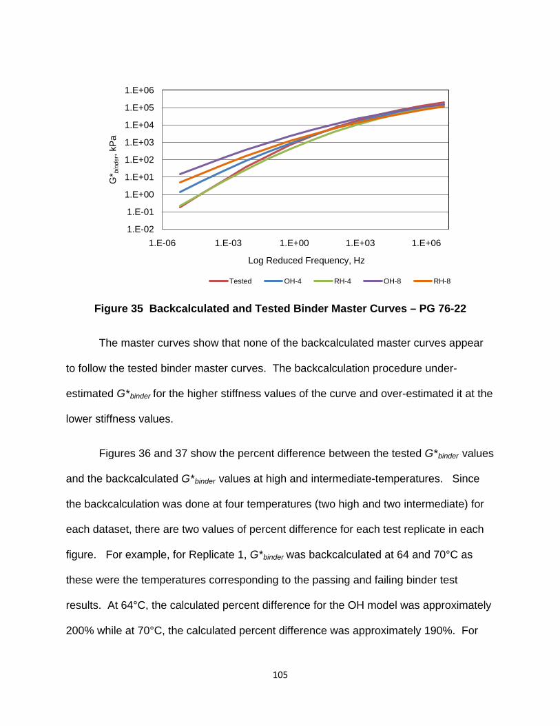
Figure 35 Backcalculated and Tested Binder Master Curves – PG 76-22
The master curves show that none of the backcalculated master curves appear
to follow the tested binder master curves. The backcalculation procedure under-
estimated G*binder for the higher stiffness values of the curve and over-estimated it at the
lower stiffness values.
Figures 36 and 37 show the percent difference between the tested G*binder values
and the backcalculated G*binder values at high and intermediate-temperatures. Since
the backcalculation was done at four temperatures (two high and two intermediate) for
each dataset, there are two values of percent difference for each test replicate in each
figure. For example, for Replicate 1, G*binder was backcalculated at 64 and 70°C as
these were the temperatures corresponding to the passing and failing binder test
results. At 64°C, the calculated percent difference for the OH model was approximately
200% while at 70°C, the calculated percent difference was approximately 190%. For
1.E-02
1.E-01
1.E+00
1.E+01
1.E+02
1.E+03
1.E+04
1.E+05
1.E+06
1.E-06 1.E-03 1.E+00 1.E+03 1.E+06
G* b
inde
r, kP
a
Log Reduced Frequency, Hz
Tested OH-4 RH-4 OH-8 RH-8
105

the RH model, the calculated percent at 64°C difference was 7% for the first
temperature and 15% at 70°C.
Figure 36 Percent Difference in G*binder for High-temperature Results- Virgin Binder
-200
0
200
400
600
800
1000
1200
1400
1600
1800
2000
1 2 3 4 5 6 7 8 9 10 11 12 13 14 15 16
% D
iffer
ence
Replicate OH RH
106

Figure 37 Percent Difference in G*binder for Intermediate-temperature Results- Virgin Binder
The figures show that at high-temperatures, both versions of the model tended to over-
estimate the backcalculated G*binder values. The RH model in most cases had lower
differences between tested and backcalculated G*binder values than the OH model;
however, the average model error was still 370%. The average model error for the OH
model was 1,285%.
At intermediate-temperatures, the differences between the two versions of the
model were not as pronounced as at the high-temperatures. Both versions of the model
tended to under-estimate G*binder at intermediate-temperatures, and in some cases the
RH model (average error = 65%) was worse than the OH model (average error = 40%).
-200
-150
-100
-50
0
50
100
150
200
1 2 3 4 5 6 7 8 9 10 11 12 13 14 15 16
% D
iffer
ence
ReplicateOH RH
107

Figures 38 - 41 compare the differences between the average backcalculated
and tested G*binder values. Results are separated by binder type, high or intermediate-
temperature range, aggregate size, and version of the model. Error bars showing the
standard deviation are included to show the high variability seen in the calculation.
Figure 38 High-temperature Backcalculated G*binder Results for PG 64-22
0
10
20
30
40
50
60
70
80
90
100
64°C 70°C
Back
-Cal
cula
ted
G* b
inde
r,kP
a
Temperature, °C
Tested Binder OH4 OH8 RH4 RH8
108

Figure 39 Intermediate-temperature Backcalculated G*binder Results for PG 64-22
Figure 40 High-temperature Backcalculated G*binder Results for PG 76-22
0
2,000
4,000
6,000
8,000
10,000
12,000
22 25
Back
-Cal
cula
ted
G* b
inde
r,kP
a
Temperature, °C
Tested Binder OH4 OH8 RH4 RH8
0
10
20
30
40
50
60
70
80
90
100
76 82
Back
-Cal
cula
ted
G* b
inde
r,kP
a
Temperature, °C
Tested Binder OH4 OH8 RH4 RH8
109

Figure 41 Intermediate-temperature Backcalculated G*binder Results for PG 76-22
Variability for the back-calculation procedure was very high in some cases, particularly
for the high-temperatures which had COV values of up to 81%. The intermediate-
temperature backcalculation results had lower COV values (between 11 and 22%). The
variability in the high-temperature results was most likely due to issues with the Hirsch
model at low mixture stiffness values.
Table 15 shows the average backcalculated G*binder values compared to the
tested G*binder values for the virgin materials. A one-sample statistical t-test (α=0.05)
was used to compare the average backcalculated results to the tested values (H0:
backcalculated G*binder = tested G*binder ). The p-values obtained from the comparisons
are included in the table.
0
2,000
4,000
6,000
8,000
10,000
12,000
22 25
Back
-Cal
cula
ted
G* b
inde
r, kP
a
Temperature, °C
Tested Binder OH4 OH8 RH4 RH8
110
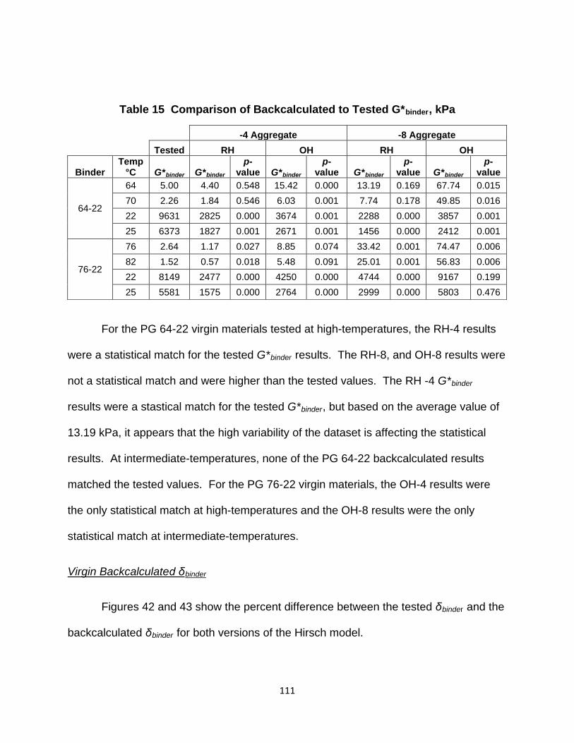
Table 15 Comparison of Backcalculated to Tested G*binder, kPa
-4 Aggregate -8 Aggregate
Tested RH OH RH OH
Binder Temp
°C G*binder G*binder p-
value G*binder p-
value G*binder p-
value G*binder p-
value
64-22
64 5.00 4.40 0.548 15.42 0.000 13.19 0.169 67.74 0.015 70 2.26 1.84 0.546 6.03 0.001 7.74 0.178 49.85 0.016 22 9631 2825 0.000 3674 0.001 2288 0.000 3857 0.001 25 6373 1827 0.001 2671 0.001 1456 0.000 2412 0.001
76-22
76 2.64 1.17 0.027 8.85 0.074 33.42 0.001 74.47 0.006 82 1.52 0.57 0.018 5.48 0.091 25.01 0.001 56.83 0.006 22 8149 2477 0.000 4250 0.000 4744 0.000 9167 0.199 25 5581 1575 0.000 2764 0.000 2999 0.000 5803 0.476
For the PG 64-22 virgin materials tested at high-temperatures, the RH-4 results
were a statistical match for the tested G*binder results. The RH-8, and OH-8 results were
not a statistical match and were higher than the tested values. The RH -4 G*binder
results were a stastical match for the tested G*binder, but based on the average value of
13.19 kPa, it appears that the high variability of the dataset is affecting the statistical
results. At intermediate-temperatures, none of the PG 64-22 backcalculated results
matched the tested values. For the PG 76-22 virgin materials, the OH-4 results were
the only statistical match at high-temperatures and the OH-8 results were the only
statistical match at intermediate-temperatures.
Virgin Backcalculated δbinder
Figures 42 and 43 show the percent difference between the tested δbinder and the
backcalculated δbinder for both versions of the Hirsch model.
111

Figure 42 Percent Difference in δbinder for High-temperature Results
Figure 43 Percent Difference in δbinder for Intermediate-temperature Results
-100-80-60-40-20
020406080
100
1 2 3 4 5 6 7 8 9 10 11 12 13 14 15 16
% D
iffer
ence
Replicate OH RH
-100-80-60-40-20
020406080
100
1 2 3 4 5 6 7 8 9 10 11 12 13 14 15 16
% D
iffer
ence
Replicate OH RH
112
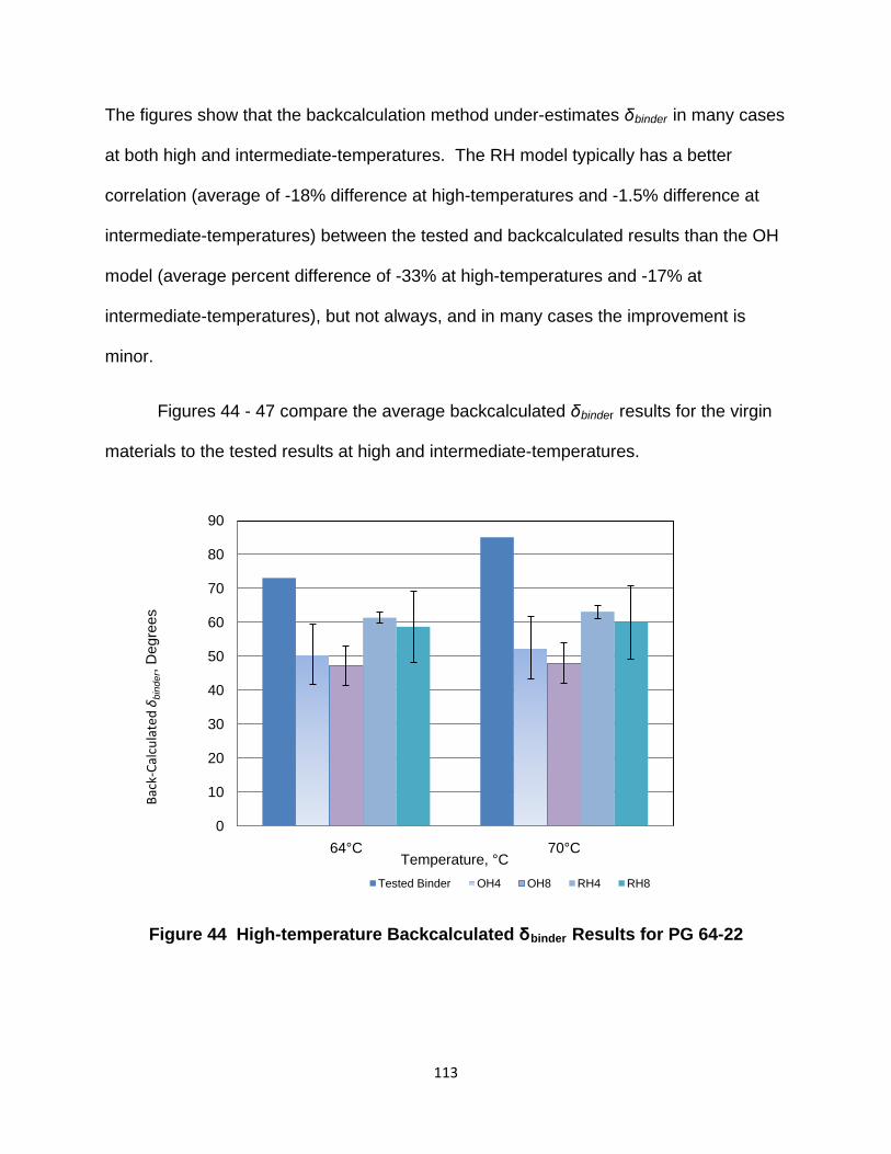
The figures show that the backcalculation method under-estimates δbinder in many cases
at both high and intermediate-temperatures. The RH model typically has a better
correlation (average of -18% difference at high-temperatures and -1.5% difference at
intermediate-temperatures) between the tested and backcalculated results than the OH
model (average percent difference of -33% at high-temperatures and -17% at
intermediate-temperatures), but not always, and in many cases the improvement is
minor.
Figures 44 - 47 compare the average backcalculated δbinder results for the virgin
materials to the tested results at high and intermediate-temperatures.
Figure 44 High-temperature Backcalculated δbinder Results for PG 64-22
0
10
20
30
40
50
60
70
80
90
64°C 70°C
Back
-Cal
cula
ted δ b
inde
r, D
egre
es
Temperature, °CTested Binder OH4 OH8 RH4 RH8
113

Figure 45 Intermediate-temperature Backcalculated δbinder Results for PG 64-22
Figure 46 High-temperature Backcalculated δbinder Results for PG 76-22
0
10
20
30
40
50
60
22 25
Back
-Cal
cula
ted δ b
inde
r, D
egre
es
Temperature, °C
Tested Binder OH4 OH8 RH4 RH8
0
10
20
30
40
50
60
70
80
90
76 82
Back
-Cal
cula
ted δ b
inde
r, D
egre
es
Temperature, °C
Tested Binder OH4 OH8 RH4 RH8
114

Figure 47 Intermediate-temperature Backcalculated δbinder Results for PG 76-22
A one-sample t-test (α=0.05) was used to compare the backcalculated δbinder
values to the tested δbinder values. Results of the statistical analysis are shown in Table
16 along with a summary of the average δbinder results for each dataset.
0
10
20
30
40
50
60
22 25
Back
-Cal
cula
ted δ b
inde
r, D
egre
es
Temperature, °C
Tested Binder OH4 OH8 RH4 RH8
115

Table 16 Comparison of Backcalculated to Tested δbinder, °
-4 Aggregate -8 Aggregate
Tested RH OH RH OH
Binder Temp,
°C δbinder, δbinder p-
value δbinder p-
value δbinder p-
value δbinder p-
value
64-22
64 73.1 61.4 0.007 50.6 0.014 58.7 0.073 46.2 0.003 70 85.1 63.2 0.003 52.5 0.006 60.0 0.019 46.9 0.001 22 40.4 44.5 0.324 34.1 0.124 41.2 0.822 33.6 0.032 25 43.3 46.8 0.430 35.4 0.081 43.2 0.982 35.4 0.030
76-22
76 69.3 67.2 0.722 53.8 0.009 45.8 0.001 44.3 0.003 82 71.5 68.8 0.664 54.7 0.007 46.4 0.000 44.9 0.063 22 39.7 41.6 0.335 35.8 0.061 31.6 0.003 30.0 0.010 25 42.0 43.7 0.419 37.6 0.056 33.4 0.004 31.8 0.012
When compared to the tested δbinder results, none of the backcalculated datasets
showed a consistent statistical match. The RH-4 dataset had the best results with
statistical matches for all but the PG 64-22 high-temperature dataset. The OH-4
dataset only showed a statistical match between tested and backcalculated δbinder for
the intermediate-temperatures. The RH-8 dataset correctly estimated δbinder for three
out of four temperatures for the PG 64-22 binder, but was not a statistical match for the
PG 76-22 δbinder at any temperature. The OH-8 dataset only had one statistical match.
Virgin Binder Critical Temperatures
Figures 48 and 49 show how the estimated binder critical temperatures
compared to the tested values for the virgin materials.
116

Figure 48 PG 64-22 Backcalculated Tcrit
Figure 49 PG 76-22 Backcalculated Tcrit
0.0
20.0
40.0
60.0
80.0
100.0
120.0
140.0
160.0
180.0
200.0
Tcrit, High Tcrit, Int
Tem
pera
ture
, °C
Binder OH4 OH8 RH4 RH8
0.0
20.0
40.0
60.0
80.0
100.0
120.0
140.0
160.0
180.0
200.0
Tcrit, High Tcrit, Int
Tem
pera
ture
, °C
Binder OH4 OH8 RH4 RH8
117

Table 17 shows the results of a one-sample t-test (α=0.05) analysis comparing
the high and intermediate backcalculated critical temperatures to the tested values.
Table 17 p-Values for Comparison of Backcalculated Critical Temperature, °C
-4 Aggregate -8 Aggregate
OH RH OH RH
Binder Temp. Tested Tcrit p-
value Tcrit p-
value Tcrit p-
value Tcrit p-
value
64-22
High 70.2 77.8 0.001 68.3 0.490 126.9 0.003 82.4 0.198 Int 23.9 31.7 0.002 31.3 0.000 28.2 0.021 31.3 0.021
76-22
High 78.6 94.5 0.041 71.0 0.066 158.2 0.001 137.1 0.000 Int 21.6 27.5 0.006 30.2 0.002 22.9 0.207 27.2 0.001
For both binders, the statistical analysis shows that there are only four statistical
matches between the tested and backcalculated Tcrit values for either model: RH-4 at
high-temperatures for both binders, OH-8 at intermediate-temperatures for the PG 76-
22, and RH-8 for the PG 64-22 at high-temperatures.
It is important to remember that the desired result of this project was a method to
estimate the properties of the binder in the torsion bar specimens. Although an exact
statistical match for the tested values would be ideal, it is not necessarily required as
long as the backcalculated results are reasonably close to the tested results. Table 18
shows the high and intermediate PG grades of the virgin binders based on the average
backcalculated results. Note that the intermediate critical temperature is not normally
stated as part of the PG grade of the binder and therefore does not have standard
values. For the sake of comparison, a value equal to the higher standard DSR test
temperature (25, 28, 31, etc) bracketing the critical temperature was assigned as the
intermediate PG grade. For example, a critical temperature of 29.1°C would be
assigned a standard value of 31.
118

Table 18 Standard PG Grades for Virgin Materials
PG 64-22 PG 76-22
High Intermediate High Intermediate Binder 70 25 76 22 OH-4 76 34 94 28 OH-8 124 31 154 25 RH-4 64 31 70 31 RH-8 82 34 136 28
At high-temperatures, the RH-4 dataset was the closest match for the high standard PG
grade of both binders, although it under-estimated the critical temperature by one
standard grade for both binders. All the other datasets significantly over-estimated the
high PG grades, sometimes by as many as thirteen grades. At intermediate-
temperatures, both versions of the model estimated PG grades that were higher than
the binder PG grade; although all were within three standard grades.
RAP Torsion Bars Back-Calculation Results
This section discusses the backcalculated results obtained for the 100% RAP
torsion bar specimens. The analysis was similar to the virgin binder back-calculation
results except that only one aggregate size was used. Also, instead of RTFO-aged
binder, the backcalculated results were compared to the values obtained from testing
the asphalt binder that was extracted and recovered from the RAP materials.
RAP Backcalculated G*binder
Figures 50 and 51 compare the backcalculated G*binder results to the tested
G*binder obtained from the extracted binders.
119

Figure 50 Comparison of Tested G*binder and Backcalculated G*binder – OH
Figure 51 Comparison of Tested and Backcalculated G*binder – RH
The comparison of RAP backcalculated and tested G*binder values looks similar to that of
the virgin binder results. The data follow a linear trend for a portion of the curve, but not
at the ends. The RAP torsion bars were stiffer than the virgin torsion bars and therefore
did not have as many issues with back-calculation at the lower frequencies, although
1.E+001.E+011.E+021.E+031.E+041.E+051.E+061.E+071.E+08
1.E+00 1.E+02 1.E+04 1.E+06 1.E+08G* b
inde
r, Ba
ck-C
alcu
late
d, k
Pa
G*binder, Tested, kPa
1.E-011.E+001.E+011.E+021.E+031.E+041.E+051.E+061.E+071.E+08
1.E+00 1.E+02 1.E+04 1.E+06 1.E+08
G* b
inde
r, Ba
ck-C
alcu
late
d, k
Pa
G*binder, Tested, kPa
120

there is still some scatter in the low stiffness data. The backcalculated values had the
same sharp increase in the higher stiffness range. Since there were more than enough
data points available to form the master curves for these test results, backcalculated
data points that appeared to be beyond the capability of the model were removed. In
most cases this was the entire 20°C data set for the RAP binders.
Figures 52 and 53 show the percent difference between the individual tested
G*binder values and the G*binder values backcalculated using both versions of the Hirsch
model. The results shown were backcalculated at the same temperatures as the
recovered RAP binder testing.
Figure 52 Percent Difference in G*binder for High-temperature Results-100% RAP
-2000
200400600800
100012001400160018002000
1 2 3 4 5 6 7 8 9 10 11 12 13 14 15 16 17 18 19 20
% D
iffer
ence
ReplicateOH RH
121

Figure 53 Percent Difference in G*binder for Intermediate-temperature Results-100% RAP
As with the virgin torsion bar results, the OH model over-estimated G*binder at
high-temperatures for the 100% RAP samples, in some cases by over 2,000% with an
average percent difference for the OH model results of 1,980%. Using the RH model
reduced the average percent difference at high-temperatures to 430%. At intermediate-
temperatures, the OH model over-estimated almost all of the G*binder values by an
average of 230% while the RH model under-estimated them by an average of 20%.
Figures 54 and 55 compare the average backcalculated G*binder values to those
obtained by testing the extracted and recovered binder for RAP 1. Error bars showing
the standard deviations of the test results are included to show the high variability seen
in the backcalculated results. The results for the other four RAP sources were similar
and are included in Appendix E.
-100
100
300
500
700
900
1 2 3 4 5 6 7 8 9 10 11 12 13 14 15 16 17 18 19 20
% D
iffer
ence
ReplicateOH RH
122
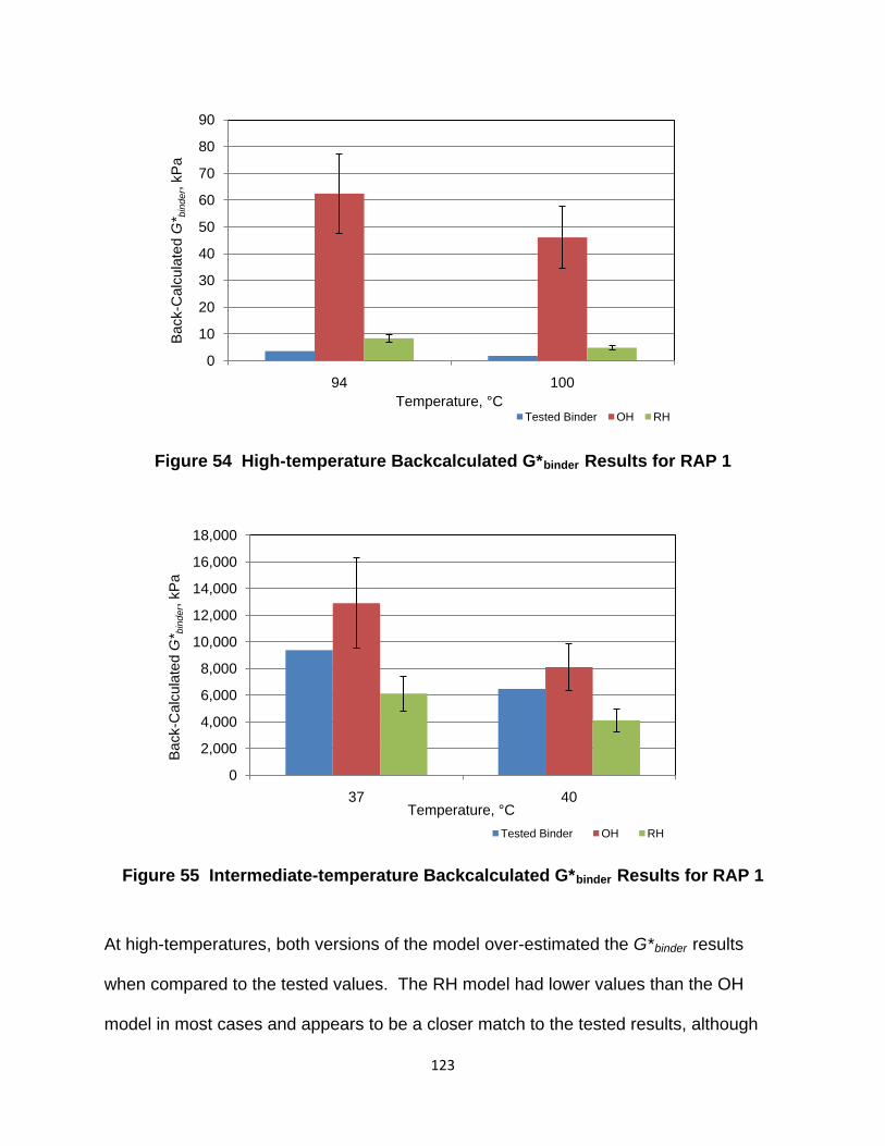
Figure 54 High-temperature Backcalculated G*binder Results for RAP 1
Figure 55 Intermediate-temperature Backcalculated G*binder Results for RAP 1
At high-temperatures, both versions of the model over-estimated the G*binder results
when compared to the tested values. The RH model had lower values than the OH
model in most cases and appears to be a closer match to the tested results, although
0
10
20
30
40
50
60
70
80
90
94 100
Back
-Cal
cula
ted
G* b
inde
r, kP
a
Temperature, °CTested Binder OH RH
0
2,000
4,000
6,000
8,000
10,000
12,000
14,000
16,000
18,000
37 40
Back
-Cal
cula
ted
G* b
inde
r, kP
a
Temperature, °CTested Binder OH RH
123

they may not be a statistical match. Both versions of the model have high variability
between the replicate data, with COV values approaching 80% in some cases.
At intermediate-temperatures, the OH model over-estimated G*binder for all five
RAPs. The RH model under-estimated G*binder for all the RAP materials except RAP 5.
Variability was high for these results as well. Neither version of the model stands out as
a consistent best match for the intermediate-temperature G*binder tested values. Table
19 shows the one-sample t-test results (α=0.05) for comparing the tested values to the
backcalculated values for each model.
124

Table 19 p-values for RAP G*binder
G*binder, kPa
RAP Temp, °C Binder OH p-value RH p-value
1
94 3.61 62.41 0.004 8.37 0.007 100 1.83 46.05 0.005 4.84 0.006 37 9380 12903 0.128 6129 0.016 40 6475 8113 0.164 4117 0.011
2
88 3.32 23.54 0.120 3.47 0.867 94 1.65 16.57 0.127 1.95 0.610 31 8735 9994 0.516 5016 0.020 34 6591 6295 0.780 3203 0.006
3
94 2.43 18.14 0.012 53.02 0.021 100 1.24 11.94 0.016 37.31 0.027 31 9410 6621 0.164 12986 0.055 34 6730 4717 0.136 9181 0.041
4
82 4.19 3.74 0.007 23.79 0.727 88 2.00 1.64 0.010 13.76 0.611 28 9732 8424 0.047 16510 0.229 31 6942 5733 0.053 10834 0.118
5
82 3.30 39.03 0.006 108.84 0.008 88 1.67 25.43 0.012 77.35 0.020 25 9018 31996 0.142 121559 0.071 28 6305 19195 0.058 55578 0.039
The statistical analysis comparing the backcalculated G*binder values and the tested
G*binder values for the RAP materials showed that at high-temperatures, neither model
was a statistical match for G*binder except for the OH model for RAP 2 and the RH model
for RAPs 2 and 4. The average results for the RAP 2 G*binder backcalculated using the
OH model and the RAP 4 G*binder backcalculated using the RH model appear to be
much larger than the average recovered binder values for these RAP sources. Both of
these datasets had extremely high COV values at high temperatures (83% for RAP 2
and 70% for RAP 4). The variability in these results is most likely affecting the results of
125

the statistical analysis in this case and it is likely that these backcalculated values are
not actually equal to the tested values.
At intermediate-temperatures, the OH G*binder dataset is the best match for all the
RAPs. The RH model is also a statistical match for RAP 4 (both temperatures) and
RAPs 3 and 5 (one temperature only) at intermediate-temperatures.
RAP Backcalculated δbinder
Figures 56 and 57 show the percent difference between the tested δbinder and the
backcalculated δbinder for the 100% RAP results using both versions of the Hirsch model.
Figure 56 Percent Difference in δbinder for HighTemperature Results
-100-80-60-40-20
020406080
100
1 2 3 4 5 6 7 8 9 10 11 12 13 14 15 16 17 18 19 20
% D
iffer
ence
ReplicateOH RH
126

Figure 57 Percent Difference in δbinder for Intermediate-temperature Results
Similar to the virgin material results, both versions of the Hirsch model under-estimated
δbinder for the 100% RAP materials at high-temperatures with the RH model (average
percent difference = -53%) as being worse than the OH model (average % difference =
-42%). At intermediate-temperatures, some of the test results are under-estimated and
some are over-estimated. In most cases, the RH model was slightly closer to the tested
values than the OH model. Both versions of the model had average percent differences
of approximately 5%.
Figures 58 and 59 compare the backcalculated δbinder values to those obtained
from testing the recovered RAP binders. RAP 1 is shown while the other RAP source
results are included in Appendix D. Trends were similar for all the RAP sources.
-100-80-60-40-20
020406080
100
1 2 3 4 5 6 7 8 9 10 11 12 13 14 15 16 17 18 19 20
% D
iffer
ence
ReplicateOH RH
127

Figure 58 High-temperature Backcalculated δbinder Results for RAP 1
Figure 59 Intermediate-temperature Backcalculated δbinder Results for RAP 1
0
10
20
30
40
50
60
70
80
90
94 100
Back
-Cal
cula
tedδ b
inde
r, °
Temperature, °CTested Binder OH RH
05
101520253035404550
37 40
Back
-Cal
cula
ted
δ bin
der,
°
Temperature, °CTested Binder OH RH
128

At high-temperatures neither model was a close match for the tested binder data, with
RAP 2 being the only exception. The models do a better job of estimating δbinder at
intermediate-temperatures. Table 20 shows the one-sample t-test results (α=0.05)
comparing the tested and calculated δbinder results.
Table 20 p-values for Backcalculated δbinder
δbinder, °
RAP Temp, °C Binder OH p-value RH p-value
1
94 80.2 47.9 0.000 51.4 0.000
100 82.5 48.0 0.000 51.7 0.000
37 40.7 42.3 0.481 39.5 0.040
40 43.4 43.3 0.959 40.9 0.006
2
88 79.9 54.3 0.000 57.4 0.000
94 82.5 54.7 0.000 58.0 0.000
31 36.1 40.0 0.055 40.9 0.020 34 37.8 42.0 0.058 42.7 0.024
3
94 80.3 40.9 0.015 43.6 0.501
100 82.9 41.3 0.012 44.1 0.466 31 36.4 29.1 0.051 30.8 0.658
34 38.8 30.3 0.087 31.9 0.794
4
82 78.7 49.1 0.000 59.4 0.013
88 81.6 49.6 0.000 60.7 0.015 28 35.5 33.4 0.027 37.0 0.055
31 37.7 35.3 0.028 38.9 0.058
5
82 80.3 44.2 0.000 46.9 0.000
88 82.8 44.4 0.000 47.3 0.000 25 37.9 32.2 0.245 30.1 0.004
28 40.4 34.4 0.167 32.4 0.004
Based on the statistical analysis of the δbinder results, only the RAP 3 δbinder dataset
calculated using the RH model was a statistical match for the tested δbinder values at
high-temperatures. Based on the average values for RAP 3, the statistical match is
129

most likely due to sample variability. All the other δbinder datasets were lower than the
tested values. At intermediate-temperatures, the δbinder values calculated for all the
RAPs except RAP 4 using the OH dataset were statistical matches for the tested δbinder
values. The RH dataset was a statistical match for RAPs 3 and 4 at intermediate-
temperatures.
RAP Critical Temperatures
Figure 60 shows how the backcalculated binder critical temperatures values
compared to the tested values for RAP 1.
Figure 60 RAP 1 Backcalculated Tcrit
Table 21 shows the one-sample t-test results (α=0.05) comparing the high and
intermediate backcalculated critical temperatures to the tested values.
0
20
40
60
80
100
120
140
160
180
200
Tcrit, High Tcrit, Int
Tem
pera
ture
, °C
Binder Original Hirsch Revised Hirsch
130

Table 21 p-Values for Comparison of Backcalculated Critical Temperature, °C
OH RH
Tested Tcrit p-value Tcrit p-value
RAP 1 High 98.4 164.9 0.001 111.1 0.001 Int 38.9 33.5 0.007 39.2 0.762
RAP 2 High 91.8 126.2 0.040 93.8 0.487 Int 31.3 29.7 0.301 34.5 0.102
RAP 3 High 95.0 152.8 0.003 127.7 0.006 Int 32.2 29.2 0.104 35.3 0.118
RAP 4 High 87.3 110.4 0.002 82.1 0.045 Int 29.4 23.4 0.010 30.1 0.633
RAP 5 High 85.7 150.8 0.009 125.9 0.015 Int 26.0 12.4 0.002 17.2 0.005
At high-temperatures, the RH dataset provided backcalculated critical temperatures that
were not a statistical match for the tested critical temperatures for any of the RAP
sources except for RAP 2. At intermediate-temperatures, the RH results were a
statistical match for all of the RAPs except for RAP 5. The critical temperatures
calculated based on the OH results were statistical matches only for RAPs 2 and 4 at
intermediate-temperatures.
As for the virgin materials, it is important to remember that the desired result of
this project was a method for estimating the binder properties of the RAP sources, not
necessarily to obtain an exact statistical match. Table 22 shows the high and
intermediate PG grades of the RAP binders based on the average of the backcalculated
results.
131

Table 22 Standard PG Grades for RAP Materials
RAP 1 RAP 2 RAP 3 RAP 4 RAP 5
High Int High Int High Int High Int High Int
Binder 94 40 88 34 94 34 82 31 82 28
OH 160 34 124 31 148 31 106 25 148 13
RH 106 40 88 37 124 37 82 31 124 19
At high-temperatures, the RH dataset did the best job of estimating the high standard
PG grade of the RAP binders, although it was off by as many as seven standard grades
in some cases. At intermediate-temperatures, the RH datasets were within one
standard temperature of the intermediate-temperature grade for all the RAP sources
except for RAP 5. The OH dataset over-estimated the high PG grade by a minimum of
four and up to eleven standard grades. The intermediate-temperature PG grades were
within two standard grades for all but RAP 5.
Summary
Based on the results presented in this chapter, the following conclusions can be
made:
1. The original version of the Hirsch model was not calibrated for the DSR torsion
bars and could not accurately predict G*mix using G*binder for either the virgin
materials or the 100% RAP materials. A calibration of the model based on the
virgin materials showed that the accuracy of the model compared to the tested
G*mix results could be improved.
132

2. The original version of the Hirsch model over-estimated G*binder at high-
temperatures by as much as 2,000% for some samples. The revised version of
the model also tended to over-estimate G*binder at high-temperatures but in most
cases was not as severe (40 – 65%). δbinder was almost always under-estimated
by both versions of the model and was usually better estimated using the original
model results.
3. At intermediate-temperatures, the virgin G*binder values were all over-estimated by
as much as 65% with no clear trend as to which version of the model is better.
The original Hirsch model severely over-estimated the RAP G*binder as well, while
the revised model under-estimated it for all but one RAP source. δbinder also
showed no clear trend at intermediate-temperatures as to which version of the
Hirsch model was better.
4. When analyzing the estimated PG grades for the virgin binders, the results
backcalculated using the revised version of the Hirsch model with the -4
aggregate gave to the closest estimate for the high and intermediate PG grade
for both virgin binders. The PG 64-22 binder (which actually graded to be PG
70+25 based on its high and intermediate temperature properties) was estimated
to be a PG 64+31(high and intermediate PG grades) based on the
backcalculated results. The PG 76-22 binder (PG 76+22 based on its high and
intermediate temperature properties) was estimated to be a PG 70+31.
5. The revised Hirsch model gave a closer estimate of the extracted binder RAP PG
grades compared to the original Hirsch model results.
133

LABORATORY RAP BLENDS AND PLANT MIXES
A potential application for the torsion bar back-calculation procedure is the
characterization of asphalt binder properties of HMA mixtures containing RAP.
Currently there is no method for directly testing the asphalt binder properties of RAP
blends other than using solvent extraction and recovery procedures to obtain the binder
to test or by estimating the asphalt binder properties from blending charts (which also
require recovered asphalt binder). If the backcalculation procedure can successfully
identify the asphalt binder properties of mixes with RAP, then it may eliminate the need
for asphalt binder testing to quantify changes in mixture stiffness due to increasing RAP
content or to identify the maximum amount of RAP that can be added to a mix while still
maintaining a target PG binder grade.
In this section of the project, the virgin and recovered binder high and
intermediate critical temperatures obtained during previous testing were used to create
blending charts for three of the RAP materials (RAP 2, RAP 3, and RAP 5). The
recovered values were used instead of the backcalculated since this is the current
method of creating blending charts according to AASHTO M323. Torsion bars made
from laboratory HMA mixes containing three different percentages of RAP (20, 35, and
50%) were tested and their binder properties backcalculated using both versions of the
model. The backcalculated values were compared to the critical temperatures
estimated by the blending charts. Five plant-produced mixes were also tested to see
how their backcalculated binder properties compared to the blending chart estimations.
134

Laboratory RAP Blends
The laboratory RAP blend evaluation was conducted using laboratory-produced
mixes containing three of the RAP sources from the previous section. Mix designs were
created using three percentages of RAP and test specimens were fabricated using both
virgin binders. Aggregate gradations for the mixes were designed to be as similar as
possible, accounting for the additional RAP aggregates. Figures 61-64 show an
example of the master curves created from the average backcalculated G*binder values
for RAP 2 with the virgin PG 64-22 binders. Also included in the figures are the G*binder
master curves obtained from testing the recovered RAP 2 binder and the RTFO-aged
virgin binder master curves. No recovery testing was done for these mixes; therefore,
there are no master curves shown for the recovered asphalt binders from the individual
blends.
135

Figure 61 PG 64-22 RAP 2 Master Curve – OH Model
Figure 62 PG 64-22 RAP 2 Master Curve – RH Model
1.E-02
1.E-01
1.E+00
1.E+01
1.E+02
1.E+03
1.E+04
1.E+05
1.E+06
1.E-06 1.E-04 1.E-02 1.E+00 1.E+02 1.E+04 1.E+06
G* b
inde
r, kP
a
Log Reduced Frequency, Hz
PG 64-22 OH 20% OH 35% OH 50% 100% RAP 2
1.E-02
1.E-01
1.E+00
1.E+01
1.E+02
1.E+03
1.E+04
1.E+05
1.E+06
1.E-06 1.E-04 1.E-02 1.E+00 1.E+02 1.E+04 1.E+06
G* b
inde
r, kP
a
Reduced Frequency, HzPG 64-22 RH 20% RH 35% RH 50% 100% RAP 2
136

Figure 63 PG 76-22 RAP 2 Master Curve – OH Model
Figure 64 PG 76-22 RAP 2 Master Curve – RH Model
1.E-02
1.E-01
1.E+00
1.E+01
1.E+02
1.E+03
1.E+04
1.E+05
1.E+06
1.E-06 1.E-04 1.E-02 1.E+00 1.E+02 1.E+04 1.E+06
G* b
inde
r, kP
a
Log Reduced Frequency, Hz
PG 76-22 OH 20% OH 35% OH 50% 100% RAP 2
1.E-02
1.E-01
1.E+00
1.E+01
1.E+02
1.E+03
1.E+04
1.E+05
1.E+06
1.E-06 1.E-04 1.E-02 1.E+00 1.E+02 1.E+04 1.E+06
G* b
inde
r, kP
a
Log Reduced Frequency, Hz
PG 76-22 RH 20 RH 35% RH 50% 100% RAP 2
137

Trends for the other RAP blends were similar and the master curves for RAPs 3 and 5
are included in Appendix E, along with a summary of the backcalculated G*binder and
δbinder results. The expected behavior for RAP mixes is increased stiffness with
increasing RAP content with the stiffness values for the blends being somewhere
between the virgin and 100% RAP binder values. Neither version of the model appears
to consistently rank the results from the different RAP contents in the expected manner
for the RAP blends. In a few cases, the G*binder values backcalculated using the RH
model for the RAP blends are softer than the virgin binder values. In other cases, the
backcalculated G*binder values are stiffer than the recovered RAP binder master curve.
In several cases, the 35% RAP blends appear to be stiffer than the 50% RAP blends.
Figure 65 shows the blending chart created for the laboratory blends containing
RAP 2 and the PG 64-22 virgin binder. The high and intermediate critical temperatures
for the virgin binder (0%) RAP and the recovered RAP 2 binder (100% RAP) were
plotted on the chart and lines drawn from the 0 to 100% RAP conditions. From these
lines, estimates were made for the high and intermediate critical temperatures at 20, 35,
and 50% RAP. For the RAP 2 blends shown in Figure 65, the estimated high critical
temperatures were found to be higher than the backcalculated critical temperatures.
Blending charts for the other RAP sources are included in Appendix F.
138

Figure 65 PG 64-22 RAP 2 Blending Chart
As can be seen from the figure, the back-calculation procedure was not
successful at estimating the high-temperature binder properties of the RAP blends
compared to the blending charts. For both versions of the Hirsch model, the high critical
temperatures based on the backcalculated results were significantly lower than those
estimated from the blending charts. For RAP 2, the backcalculated high critical
temperatures are also not following the expected trends of increasing values with
increasing RAP contents and are lower at 50% RAP than at the 35% and the 20%
values.
At intermediate-temperatures, the backcalculated critical temperature results are
a better match for the values estimated from the blending charts. A one-sample t-test
0.0
10.0
20.0
30.0
40.0
50.0
60.0
70.0
80.0
90.0
100.0
0 20 40 60 80 100
T crit
, °C
% RAPPG 64-22 high PG 64-22 int original HIrschRevised Hirsch original Hirsch int Revised Hirsch Int
139

analysis (α=0.05) was used to compare the critical temperatures estimated from the
blending charts to the backcalculated values for all the RAP and virgin binder
combinations. Tables 23 and 24 show the average estimated and backcalculated
critical temperatures and the p-values obtained from the statistical analysis.
Table 23 p-values for Laboratory RAP Blends with PG 64-22
PG 64-22
Blending OH RH
% RAP Range Chart Tcrit Tcrit p-value Tcrit p-value
RAP2
20% High 74.5 63.2 0.009 56.9 0.003 Int 25.4 23.5 0.188 26.6 0.327
35% High 77.7 64.0 0.002 56.6 0.001 Int 26.5 24.6 0.024 27.8 0.102
50% High 80.9 60.2 0.000 55.8 0.001 Int 27.6 23.8 0.029 26.8 0.202
RAP 3
20% High 75.2 60.3 0.004 55.5 0.000 Int 25.6 23.1 0.148 26.3 0.487
35% High 78.9 73.5 0.034 63.9 0.000 Int 26.8 15.9 0.004 20.7 0.008
50% High 82.6 76.2 0.030 66.1 0.007 Int 28.1 12.5 0.002 17.4 0.004
RAP 5
20% High 73.3 63.0 0.066 62.5 0.070 Int 24.3 24.4 0.968 28.2 0.457
35% High 75.6 66.1 0.026 60.9 0.038 Int 24.6 17.7 0.003 20.6 0.006
50% High 78.0 68.3 0.014 64.7 0.001 Int 25.0 20.1 0.060 25.0 0.993
140
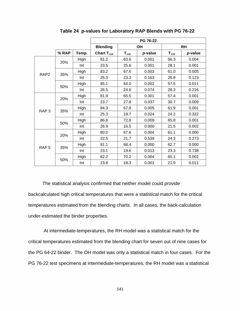
Table 24 p-values for Laboratory RAP Blends with PG 76-22
PG 76-22
Blending OH RH
% RAP Temp. Chart Tcrit Tcrit p-value Tcrit p-value
RAP2
20% High 81.2 63.6 0.001 56.3 0.004 Int 23.5 25.6 0.001 28.1 0.001
35% High 83.2 67.6 0.003 61.0 0.005 Int 25.0 23.3 0.163 26.8 0.123
50% High 85.1 64.0 0.002 57.5 0.011 Int 26.5 24.6 0.074 28.3 0.216
RAP 3
20% High 81.9 65.5 0.001 57.4 0.001 Int 23.7 27.8 0.037 30.7 0.009
35% High 84.3 67.8 0.005 61.9 0.001 Int 25.3 19.7 0.024 24.2 0.322
50% High 86.8 72.8 0.009 65.8 0.001 Int 26.9 16.5 0.000 21.5 0.002
RAP 5
20% High 80.0 67.6 0.004 61.1 0.000 Int 22.5 21.7 0.539 24.3 0.273
35% High 81.1 68.4 0.000 62.7 0.000 Int 23.1 19.6 0.013 23.3 0.738
50% High 82.2 70.2 0.004 65.1 0.002 Int 23.8 18.3 0.001 21.9 0.011
The statistical analysis confirmed that neither model could provide
backcalculated high critical temperatures that were a statistical match for the critical
temperatures estimated from the blending charts. In all cases, the back-calculation
under-estimated the binder properties.
At intermediate-temperatures, the RH model was a statistical match for the
critical temperatures estimated from the blending chart for seven out of nine cases for
the PG 64-22 binder. The OH model was only a statistical match in four cases. For the
PG 76-22 test specimens at intermediate-temperatures, the RH model was a statistical
141
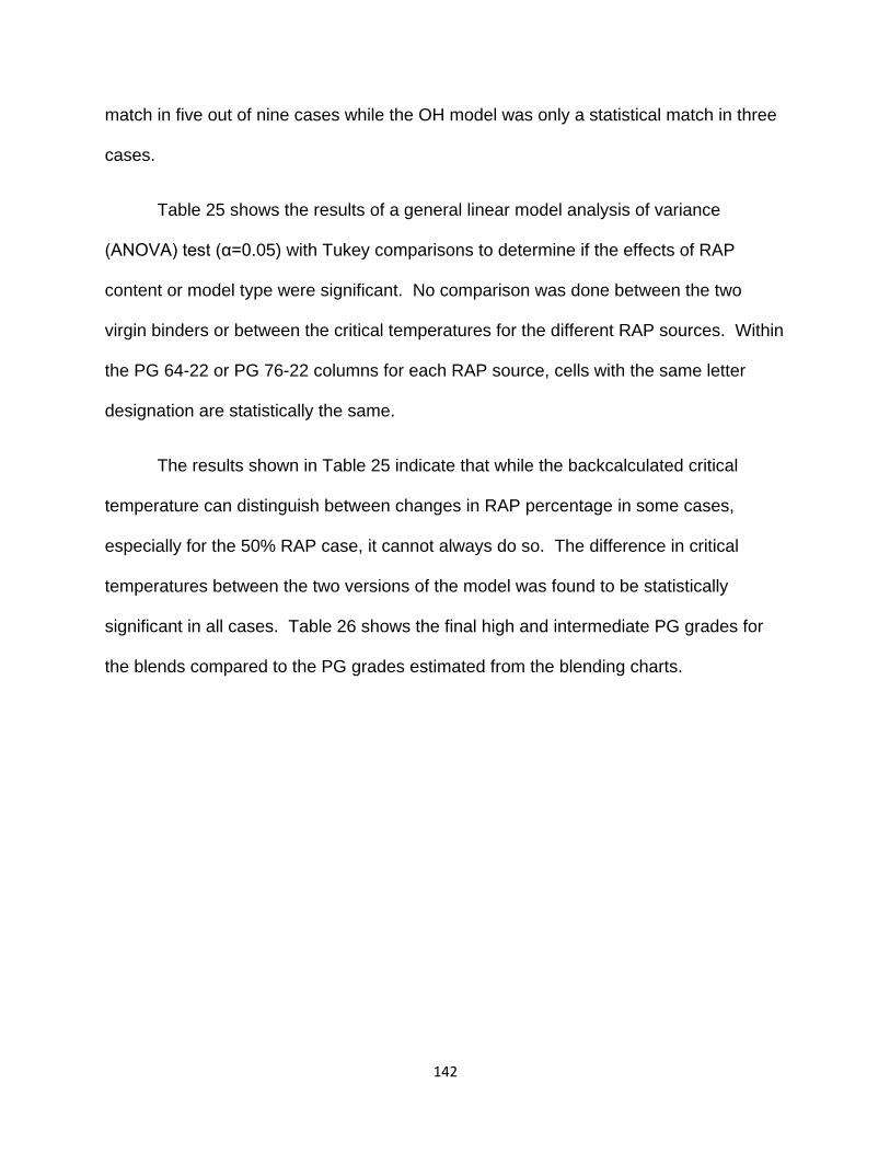
match in five out of nine cases while the OH model was only a statistical match in three
cases.
Table 25 shows the results of a general linear model analysis of variance
(ANOVA) test (α=0.05) with Tukey comparisons to determine if the effects of RAP
content or model type were significant. No comparison was done between the two
virgin binders or between the critical temperatures for the different RAP sources. Within
the PG 64-22 or PG 76-22 columns for each RAP source, cells with the same letter
designation are statistically the same.
The results shown in Table 25 indicate that while the backcalculated critical
temperature can distinguish between changes in RAP percentage in some cases,
especially for the 50% RAP case, it cannot always do so. The difference in critical
temperatures between the two versions of the model was found to be statistically
significant in all cases. Table 26 shows the final high and intermediate PG grades for
the blends compared to the PG grades estimated from the blending charts.
142

Table 25 ANOVA Results for Laboratory Blends
PG 64-22 PG 76-22
RAP, % OH RH OH RH
RAP 2
High Temps 20 A C A C 35 A C B D 50 B D B D
Int Temps 20 A B A C 35 A B AB CD 50 A B B C
RAP 3
High Temps 20 A D A D 35 B E B E 50 C F C F
Int Temps 20 A D A D 35 B E B E 50 C F C F
RAP 5
High Temps 20 A B A D 35 A B B E 50 A B C F
Int Temps 20 A C A D 35 AB CD B E 50 AB C C F
143

Table 26 PG Grades for Laboratory Blends
PG 64-22 PG 76-22
RAP, % Blending Chart OH RH Blending
Chart OH RH
RAP 2
20 70 58 52 76 58 52 35 76 64 64 82 52 58 50 76 58 64 82 52 52 20 28 25 28 25 28 31 35 28 25 25 28 28 28 50 28 25 25 28 28 31
RAP 3
20 70 58 64 76 52 52 35 76 70 64 82 58 58 50 82 76 70 82 64 64 20 28 25 28 25 28 31 35 28 16 22 28 22 25 50 31 13 19 28 19 22
RAP 5
20 70 58 64 76 58 58 35 70 64 64 76 58 58 50 76 64 70 82 64 64 20 25 22 22 25 28 25 35 25 19 22 25 22 25 50 25 22 19 25 25 22
At high-temperatures, the backcalculated PG grades were at least one grade and as
many as three grades lower than those estimated from the blending charts for all of the
blends. At intermediate-temperatures, there was no trend in the results, with some
RAP/binder combinations having lower intermediate grades than those estimated from
the blending charts and some having higher intermediate PG grades.
Plant Mix Analysis
The final portion of the project involved testing plant-produced HMA to determine
if the back-calculation method could identify the properties of the asphalt binder in the
mix. Torsion bar test specimens were constructed from five plant-produced mixes
144

containing various percentages of RAP and either a PG 64-22 or PG 76-22 virgin
binder. Asphalt binder properties were backcalculated from the torsion results and
compared to those obtained by testing asphalt binder recovered using solvent extraction
and recovery procedures. The backcalculated binder results were also compared to the
critical temperatures estimated from blending charts created using the recovered RAP
binder properties for the RAP sources used in the mixes.
Figures 66 – 69 show the backcalculated G*binder master curves compared to the
G*binder obtained from the recovered binder for four of the mixes. Plant mix C did not
have enough material to do extractions and therefore is not shown.
Figure 66 G*binder Master Curves – Plant Mix A
1.E-01
1.E+00
1.E+01
1.E+02
1.E+03
1.E+04
1.E+05
1.E+06
1.E-06 1.E-04 1.E-02 1.E+00 1.E+02 1.E+04 1.E+06
G* b
inde
r, kP
a
Log Reduced Frequency, Hz
Recovered BInder Back-calculated OH Back-calculated RH
145

Figure 67 G*binder Master Curves – Plant Mix B
Figure 68 G*binder Master Curves – Plant Mix D
1.E-01
1.E+00
1.E+01
1.E+02
1.E+03
1.E+04
1.E+05
1.E+06
1.E-06 1.E-04 1.E-02 1.E+00 1.E+02 1.E+04 1.E+06
G* b
inde
r, kP
a
Log Reduced Frequency, Hz
Recovered BInder Back-calculated OH Back-calculated RH
1.E-01
1.E+00
1.E+01
1.E+02
1.E+03
1.E+04
1.E+05
1.E+06
1.E-06 1.E-04 1.E-02 1.E+00 1.E+02 1.E+04 1.E+06
G* b
inde
r, kP
a
Log Reduced Frequency, Hz
Recovered BInder Back-calculated OH Back-calculated RH
146
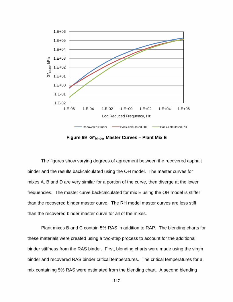
Figure 69 G*binder Master Curves – Plant Mix E
The figures show varying degrees of agreement between the recovered asphalt
binder and the results backcalculated using the OH model. The master curves for
mixes A, B and D are very similar for a portion of the curve, then diverge at the lower
frequencies. The master curve backcalculated for mix E using the OH model is stiffer
than the recovered binder master curve. The RH model master curves are less stiff
than the recovered binder master curve for all of the mixes.
Plant mixes B and C contain 5% RAS in addition to RAP. The blending charts for
these materials were created using a two-step process to account for the additional
binder stiffness from the RAS binder. First, blending charts were made using the virgin
binder and recovered RAS binder critical temperatures. The critical temperatures for a
mix containing 5% RAS were estimated from the blending chart. A second blending
1.E-02
1.E-01
1.E+00
1.E+01
1.E+02
1.E+03
1.E+04
1.E+05
1.E+06
1.E-06 1.E-04 1.E-02 1.E+00 1.E+02 1.E+04 1.E+06
G* b
inde
r, kP
a
Log Reduced Frequency, Hz
Recovered BInder Back-calculated OH Back-calculated RH
147
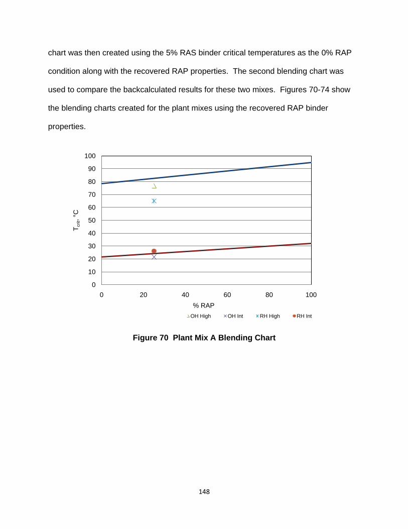
chart was then created using the 5% RAS binder critical temperatures as the 0% RAP
condition along with the recovered RAP properties. The second blending chart was
used to compare the backcalculated results for these two mixes. Figures 70-74 show
the blending charts created for the plant mixes using the recovered RAP binder
properties.
Figure 70 Plant Mix A Blending Chart
0
10
20
30
40
50
60
70
80
90
100
0 20 40 60 80 100
T crit
, °C
% RAPOH High OH Int RH High RH Int
148

Figure 71 Plant Mix B Blending Chart
Figure 72 Plant Mix C Blending Chart
0
10
20
30
40
50
60
70
80
90
100
0 20 40 60 80 100
T crit
, °C
% RAP
OH High OH Int RH High RH Int
0
10
20
30
40
50
60
70
80
90
100
0 20 40 60 80 100
T crit
, °C
% RAP
OH High OH Int RH High RH Int
149
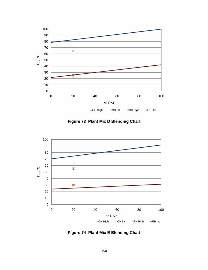
Figure 73 Plant Mix D Blending Chart
Figure 74 Plant Mix E Blending Chart
0
10
20
30
40
50
60
70
80
90
100
0 20 40 60 80 100
T crit
, °C
% RAP
OH High OH Int RH High RH Int
0
10
20
30
40
50
60
70
80
90
100
0 20 40 60 80 100
T crit
, °C
% RAPOH High OH int RH High RH int
150

The blending charts show that the backcalculated high critical temperatures for
the plant-produced mixes were usually lower than the estimated critical temperatures.
The intermediate backcalculated critical temperatures match those estimated from the
blending charts fairly well in most cases. Table 27 shows results of a one sample t-test
(α=0.05) comparison of backcalculated and estimated critical temperatures.
Table 27 p-values Comparing Backcalculated Critical Temperature to Blending Chart Values
Tcrit, High, °C Tcrit, Intermediate, °C
Mix Blending Chart OH
p-value RH
p-value
Blending Chart OH
p-value RH
p-value
A 82.7 76.9 0.079 65.1 0.005 24.3 21.6 0.072 26.2 0.234 B 75.6 68.5 0.002 60.0 0.005 24.9 23.0 0.248 27.8 0.308 C 75.1 76.8 0.030 75.1 0.972 24.6 16.7 0.002 20.8 0.012 D 82.9 70.0 0.004 65.0 0.003 25.7 21.8 0.087 25.5 0.916 E 74.5 64.1 0.001 55.2 0.001 25.4 29.0 0.008 30.3 0.002
The statistical analysis shows that only the high critical temperatures backcalculated for
plant mix A using the original Hirsch model and plant mix C using the revised Hirsch
model match the values estimated from the blending chart. All the other plant mix
backcalculated high critical temperatures were significantly lower than the blending
chart values. At intermediate-temperatures, only plant mixes C and E did not match the
blending chart values for either version of the model. Plant mixes A, B, and D
backcalculated intermediate critical temperatures were a statistical match for the
blending chart values regardless of the model used.
Table 28 shows the statistical analysis results using a 1-sample t-test (α=0. 05)
comparing the critical temperatures from the recovered binder testing and those
backcalculated from the torsion bar results.
151
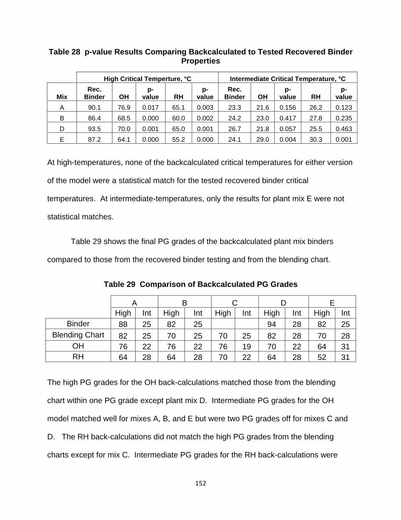
Table 28 p-value Results Comparing Backcalculated to Tested Recovered Binder Properties
High Critical Temperture, °C Intermediate Critical Temperature, °C
Mix Rec.
Binder OH p-
value RH p-
value Rec.
Binder OH p-
value RH p-
value A 90.1 76.9 0.017 65.1 0.003 23.3 21.6 0.156 26.2 0.123 B 86.4 68.5 0.000 60.0 0.002 24.2 23.0 0.417 27.8 0.235 D 93.5 70.0 0.001 65.0 0.001 26.7 21.8 0.057 25.5 0.463 E 87.2 64.1 0.000 55.2 0.000 24.1 29.0 0.004 30.3 0.001
At high-temperatures, none of the backcalculated critical temperatures for either version
of the model were a statistical match for the tested recovered binder critical
temperatures. At intermediate-temperatures, only the results for plant mix E were not
statistical matches.
Table 29 shows the final PG grades of the backcalculated plant mix binders
compared to those from the recovered binder testing and from the blending chart.
Table 29 Comparison of Backcalculated PG Grades
A B C D E High Int High Int High Int High Int High Int
Binder 88 25 82 25 94 28 82 25 Blending Chart 82 25 70 25 70 25 82 28 70 28
OH 76 22 76 22 76 19 70 22 64 31 RH 64 28 64 28 70 22 64 28 52 31
The high PG grades for the OH back-calculations matched those from the blending
chart within one PG grade except plant mix D. Intermediate PG grades for the OH
model matched well for mixes A, B, and E but were two PG grades off for mixes C and
D. The RH back-calculations did not match the high PG grades from the blending
charts except for mix C. Intermediate PG grades for the RH back-calculations were
152

within one PG grade. All the backcalculated PG grades were under-estimated
compared to those from the recovered binder tests.
Summary
The following observations were made from the results of the laboratory and plant-
produced mixes:
1. Neither version of the Hirsch model could accurately estimate the high critical
temperatures of the laboratory mixes. Both versions under-estimated the
high-temperature grade by at least one standard PG grade. In many cases,
the backcalculated critical temperature was lower than the high critical
temperature for the virgin binder. The revised Hirsch model was a better
match than the original Hirsch model for the intermediate critical
temperatures.
2. Neither version of the model could consistently identify changes in asphalt
binder stiffness due to increasing RAP content and showed the 50% RAP
case to be less stiff than the 35% case in several instances. The stiffer PG
76-22 mixes better identified changes in mix stiffness than the PG 64-22
mixes.
3. As with the laboratory mixes, both versions of the model under-estimated the
high critical temperatures of the plant mix. The revised Hirsch model
backcalculated values were lower than the original Hirsch model. At
intermediate-temperatures, the backcalculated values for both versions of the
model were more likely to be a statistical match for the blending chart critical
153
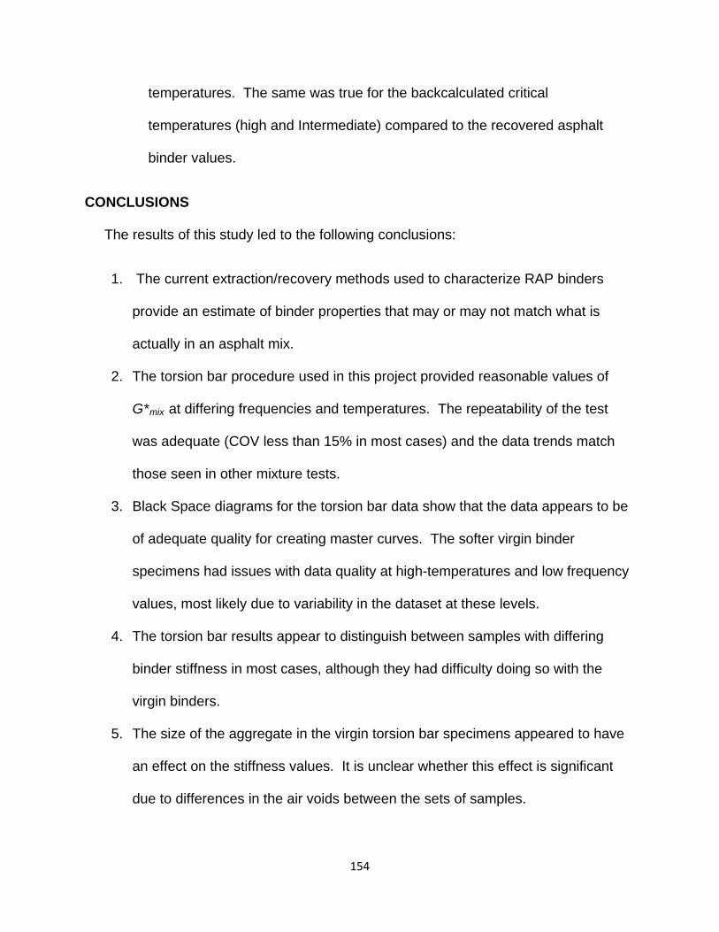
temperatures. The same was true for the backcalculated critical
temperatures (high and Intermediate) compared to the recovered asphalt
binder values.
CONCLUSIONS
The results of this study led to the following conclusions:
1. The current extraction/recovery methods used to characterize RAP binders
provide an estimate of binder properties that may or may not match what is
actually in an asphalt mix.
2. The torsion bar procedure used in this project provided reasonable values of
G*mix at differing frequencies and temperatures. The repeatability of the test
was adequate (COV less than 15% in most cases) and the data trends match
those seen in other mixture tests.
3. Black Space diagrams for the torsion bar data show that the data appears to be
of adequate quality for creating master curves. The softer virgin binder
specimens had issues with data quality at high-temperatures and low frequency
values, most likely due to variability in the dataset at these levels.
4. The torsion bar results appear to distinguish between samples with differing
binder stiffness in most cases, although they had difficulty doing so with the
virgin binders.
5. The size of the aggregate in the virgin torsion bar specimens appeared to have
an effect on the stiffness values. It is unclear whether this effect is significant
due to differences in the air voids between the sets of samples.
154

6. The original Hirsch model formula could not accurately forward calculate G*mix
using either the virgin G*binder or the recovered RAP G*binder. Calculated G*mix
values were usually under-estimated for both sets of materials.
7. A calibration of the Hirsch model using the virgin binder data resulted in a
revised model that provided an improved correlation between tested and
calculated G*mix for the virgin binder specimens. Calculation of G*mix using the
revised Hirsch model also showed an improved correlation to the tested G*mix for
the 100% RAP specimens, although the calculated values were still under-
estimated compared to the tested values.
8. Both versions of the model had problems with scatter in the backcalculated
results at the high-temperature/low frequency condition. Both versions also had
problems with the limitations of the model at low-temperature/high frequency
values and large variability between the backcalculated results compared to that
of the G*mix data (up to 83% in some cases).
9. For the virgin materials, neither verson of the model could accurately predict the
PG grade of the binders. The original Hirsch with -4 aggregate dataset (PG
76+34) or the revised Hirsch with passing -4 dataset (PG 64+31) gave the
closest estimate of PG temperature for the PG 64-22 results. The revised
Hirsch with passing -4 aggregate dataset gave the closest estimate for the PG
76-22 at high temperatures (PG 70) while the original Hirsch with passing -8
aggregate dataset gave the closest estimate at intermediate temperatures (PG
+25).
155

10. Neither of the versions of the model could accurately estimate the PG grade of
the RAP binders compared to the recovered RAP binder tests in all cases.
When estimating the PG grades for the 100% RAP materials, the revised HIrsch
model gave the closest estimate of high PG grade, with exact matches for two of
the five RAP sources. Estimated PG grades for the other three RAP sources
were within two and seven PG grades. At intermediate temperatures, both
versions of the model estimated PG grades that were within one or two grades
for all but one RAP.
11. Neither model could accurately predict the high-temperature PG grades of
laboratory or plant-produced mixes. Comparisons were made using both
blending charts and recovered binder from the actual mixes (plant mixes only).
In all cases, the backcalculated results were significantly lower than the actual
tested values.
12. Both models adequately estimated the intermediate-temperature PG grades of
the laboratory blends and plant-produced mixes. Backcalculated PG grades
were within 1 standard grade in most cases.
13. The results backcalculated from the torsion bars G*mix for the laboratory mixes
were not able to distinguish between changes in binder stiffness due to
increasing RAP content.
Overall, the torsion bar test procedure for measuring G*mix appear to be promising, but
much more work is needed to improve repeatability. The values of G*mix it provides are
of reasonable quality and provide the expected trends with changes in materials and
testing conditions. Repeatability may be improved in the future by using tighter controls
156

on air voids so that the percent of air voids does not vary by more than 0.5% between
test specimens. Air voids should also be kept to the normal ranges used in asphalt
mixture testing. The air voids seen in the torsion bars were several percent higher than
normal target values. Repeatability may also be improved by using a larger specimen
size than the 5.5-mm thick by 11.5-mm wide by 50-mm long bars used in this research.
Finally, repeatability may be improved with a better quality saw blade than the one used
to cut the tested specimens. Using the tile saw, it was difficult to cut test specimens that
had similar dimensions and flawless surfaces.
The Hirsch model back-calculation procedure may have some promise as a
means of estimating the PG grades of RAP materials, but needs much more work to
improve accuracy and reduce variability in the backcalculate data. The calibration
process described in this report improved the estimated high temperature PG grades,
but still gives values that are over- or under-estimated by at least one grade. A more
thorough calibration using multiple binder and aggregate combinations may provide a
better calibration of the model. The results obtained from the model may also be
improved by using larger test specimens with lower percentages of air voids. This will
lead to higher G*mix values which may be handled better by the model.
The back-calculation procedure does not appear to be a good candidate for
quality control of laboratory- and plant-produced mixes. The backcalculated PG grades
for the high-temperature tests did a poor job of estimating the binder properties for
these mixes and neither version of the model could consistently distinguish between
different RAP contents.
157
REFERENCES
1. “Average Cost of Asphalt Cement Based on the NCDOT Liquid Index” http://www.stwcorp.com/en/34/Default.aspx?&Year=2012.
2. “Oklahoma Department of Transportation Monthly Asphalt Binder Price Index” http://www.okladot.state.ok.us/contractadmin/pdfs/binder-index.pdf.
3. Fournier, Paul. “What’s Driving Asphalt Prices Up?” www.acppubs.com, http://www.superpave.psu.edu/downloads/pdf/What%27s%20driving%20asphalt.pdf, October, 2008.
4. “Recycled HMA” www.asphaltwa.com, http://www.asphaltwa.com/2010/09/18/pavement-types-recycled-hma, 2010.
5. “Reclaimed Asphalt Pavement” www.graniterock.com,
http://www.graniterock.com/technical_notes/reclaimed_asphalt_pavement.html
6. McDaniel, R., H. Soleymani, R. Anderson, P. Turner, and R. Peterson. NCHRP Web Document 30: Recommended Use of Reclaimed Asphalt Pavement in the Superpave Mix Design Method, Transportation Research Board, National Research Council, Washington, D.C., 2000.
7. Peterson, R.L., H.R. Soleymani, R.M. Anderson, and R.S. McDaniel. “Recovery and Testing of RAP Binders from Recycled Asphalt Pavements,” Journal of the Association of Asphalt Paving Technologists, Vol. 69, 2000.
8. VWR Scientific Price Sheet (2011).
9. Abson, G. “Method and Apparatus for the Recovery of Asphalt,” Proceedings
ASTM Vol II, 1933.
10. Burr, B.L., R.R. Davison, C.J. Glover, and J.A. Bullin. “Solvent Removal from Asphalt,” Transportation Research Record 1269, Transportation Research Board, National Research Council, Washington, D.C., 1990.
11. Soleymani, H., H. Bahia, and A. Bergan. “Time-Temperature Dependency of Blended and Rejuvenated RAP Binders,” Journal of the Association of Asphalt Paving Technologists, Vol. 68, 1999
158
12. McDaniel, S.R., and A. Shah. “Use of Reclaimed Asphalt Pavement (RAP) Under Superpave Specifications,” Journal of the Association of Asphalt Paving Technologists, Vol. 72, 2003.
13. Daniel, J.S., J.L. Pochily, and D.M. Boisvert. “Can More Reclaimed Asphalt Pavement be Added?” Transportation Research Record No. 2180, Transportation Research Board of the National Academies, Washington, D.C., 2010.
14. Hajj, E.Y., P.E. Sebaaly, L. Loria, K. Said. Kass, T. Liske. “Impact of High RAP Content on the Performance Characteristics of Asphalt Mixtures in Manitoba,” Paper presented at The Innovative Developments in Sustainable Pavements Session of the 2011 Annual Conference of the Transportation Association of Canada, 2011.
15. Mogawer, W.S., T. Bennert, J.S. Daniel, R. Bonaquist, A. Austerman, A. Booshehrian. “Performance Characteristics of Plant Produced High RAP Mixtures,” presented at the 87th Annual Meeting of the Association of Asphalt Paving Technologists, Austin, TX., 2012.
16. McDaniel, R.S., A. Shah, and G. Huber. “Investigation of Low- and High-
Temperature Properties of Plant-Produced RAP Mixtures,” FHWA-HRT-11-058, Federal Highway Administration, 2012.
17. Zhao, S., B.Huang, X.Shu, X. Jia, and M. Woods. “Laboratory Performance
Evaluation of Warm Mix Asphalt Containing High Percentages of RAP,” Paper presented at the Transportation Research Board Annual Meeting, Washington, D.C., 2012.
18. Roque, R., B. Birgisson, C. Drakos, and B. Dietrich. “Development and Field
Evaluation of Energy-Based Criteria for Top-down Cracking Performance of Hot Mix Asphalt,” Journal of the Association of Asphalt Paving Technologists, Vol. 73, 2004.
19. Zofka, A., M.O. Marasteanu, T.R. Clyne, X. Li, and O. Hoffmann. “Development of Simple Asphalt Test for Determination of RAP Blending Charts,” Report 2004-44, Minnesota Department of Transportation, St. Paul, MN, 2004.
20. Zofka, A., Mihai Marasteanu, X. Li, T. Clyne, and J. McGraw. “Simple Method to Obtain Asphalt Binders Low-temperature Properties from Asphalt Mixtures Properties,” Journal of the Association of Asphalt Paving Technologists, Vol.74, 2005.
21. Velasquez, R., M. Marasteanu, J. Labuz, and M. Turos. “Evaluation of Bending Beam Rheometer for Characterization of Asphalt Mixtures, “Journal of the Association of Asphalt Paving Technologists, Vol 79, 2010.
159

22. Bennert, T., and R. Dongre. “A Backcalculation Method to Determine Effective Asphalt Binder Properties of RAP Mixtures,” Transportation Research Record 2179, Transportation Research Board, National Research Council, Washington, D.C., 2010.
23. Tran, N., A. Taylor, R. West, and A. Kvasnak. “Evaluation of Predictive Models for Determination of Binder Critical High-temperature from Mixture Properties,” Transportation Research Record 2179, Transportation Research Board, National Research Council, Washington, D.C., 2010.
24. Swiertz, D., E. Mahmoud, and H.U. Bahia. “Estimating the Effect of Recycled Asphalt Pavements and Asphalt Shingles on Fresh Binder, Low-Temperature Properties without Extraction and Recovery,” Transportation Research Record No. 2208, Transportation Research Board of the National Academies, Washington, D.C., 2011.
25. Performance Graded Asphalt Binder Specification and Testing, Asphalt Institute Superpave Series No. 1 (SP-1), Lexington, KY., 1997.
26. Javed, B., and M.W. Witczak. “Development of a New Revised Version of the
Witczak E* Predictive Model for Hot Mix Asphalt Mixtures,” Journal of the Association of Asphalt Paving Technologists, Vol. 75, 2006.
27. Christensen, D.W., T. Pellinen, and R. Bonaquist. “Hirsch Model for Estimating the
Modulus of Asphalt Concrete,” Journal of the Association of Asphalt Paving Technologists, Vol. 72, 2003.
28. Christensen, D.W., and D.A. Anderson. “Interpretation of Dynamic Mechanical Test Data for Paving Grade Asphalt Cements, Journal of the Association of Asphalt Paving Technologists, Vol. 62, 1992.
29. Rowe, G.M., and M.J. Sharrock. “Alternate Shift Factor Relationship for Describing the Temperature Dependency of the Visco-Elastic Behaviour of Asphalt Materials,” Transportation Research Record No. 2208, Transportation Research Board of the National Academies, Washington, D.C., 2011.
30. Rowe, G. “Phase Angle Determination and Interrelationships within Bituminous
Materials,” Presented at 45th Petersen Asphalt Research Conference, Laramie, WY., 2008.
160

31. Dongre, R., L. Myers, J. D’Angelo, C. Paugh, and J. Gudimettla. “Field Evaluation of Witczak and Hirsch Models for Predicting Dynamic Modulus of Hot-Mix Asphalt,” Journal of the Association of Asphalt Paving Technologists, Vol. 74, 2005.
161

Appendix A
Figure A-1 Alabama Contractor Locations
162

Appendix B
The following section describes the process used to determine backcalculated
values of G*binder and δbinder based on DSR torsion bar results. The example calculation
shown uses the original version of the Hirsch model. The procedure used for the
revised version was identical with the exception of the formula used.
1. Obtain a set of torsion bar G*mix data as shown in Table B-1:
Table B-1 Sample Torsion Bar Results
Temp frequency |G*| delta °C Hz Pa degrees 20 0.1 1.458E+09 20.82 20 1 2.250E+09 16.92 20 10 3.251E+09 14.26 30 0.1 6.409E+08 27.65 30 1 1.139E+09 23.01 30 10 1.873E+09 19.24 40 0.1 2.695E+08 31.49 40 1 5.231E+08 28.63 40 10 9.744E+08 24.99 50 0.1 1.226E+08 32.83 50 1 2.444E+08 32.09 50 10 5.028E+08 30.44 60 0.1 5.691E+07 31.80 60 1 1.078E+08 33.87 60 10 2.297E+08 34.89
2. Create a spreadsheet as shown in Table B-2 to determine the value of
backcalculated G*binder that will provide predicted G*mix equal to measured G*mix
using equations 2 and 3. This can be done by either manually changing the
values of G*binder or by setting up a Microsoft Excel solver or goal-seek function.
163

Table B-2 Iterative Spreadsheet to solve for Backcalculated G*binder
Temp Freq Measured G*mix
Volumetrics (%)
Backcalculated G*binder Pc
Predicted G*mix Difference
(oC) (Hz) Pa (psi) VMA VFA (psi) kPa (psi)
20 0.10 1.46E+09 211465.02 15.7 53.6 1,174.7 8099.2 0.41 211465 0
20 1.00 2.25E+09 3.26E+05 15.7 53.6 4,418.8 30466.7 0.63 326335 0
20 10.00 3.25E+09 4.72E+05 15.7 53.6 47,747.8 329209.2 0.90 471518 0
30 0.10 6.41E+08 9.30E+04 15.7 53.6 215.2 1484.0 0.18 92955 0
30 1.00 1.14E+09 1.65E+05 15.7 53.6 663.3 4573.1 0.32 165198 0
30 10.00 1.87E+09 2.72E+05 15.7 53.6 2,342.1 16148.1 0.53 271656 0
40 0.10 2.70E+08 3.91E+04 15.7 53.6 49.6 342.2 0.08 39088 0
40 1.00 5.23E+08 7.59E+04 15.7 53.6 150.3 1036.0 0.15 75869 0
40 10.00 9.74E+08 1.41E+05 15.7 53.6 478.2 3296.9 0.28 141325 0
50 0.10 1.23E+08 1.78E+04 15.7 53.6 14.0 96.2 0.04 17782 0
50 1.00 2.44E+08 3.54E+04 15.7 53.6 42.4 292.1 0.07 35447 0
50 10.00 5.03E+08 7.29E+04 15.7 53.6 140.3 967.3 0.14 72925 0
60 0.10 5.69E+07 8.25E+03 15.7 53.6 3.8 26.0 0.02 8254 0
60 1.00 1.08E+08 1.56E+04 15.7 53.6 11.3 78.0 0.03 15635 0
60 10.00 2.30E+08 3.33E+04 15.7 53.6 38.3 264.3 0.07 33315 0
164
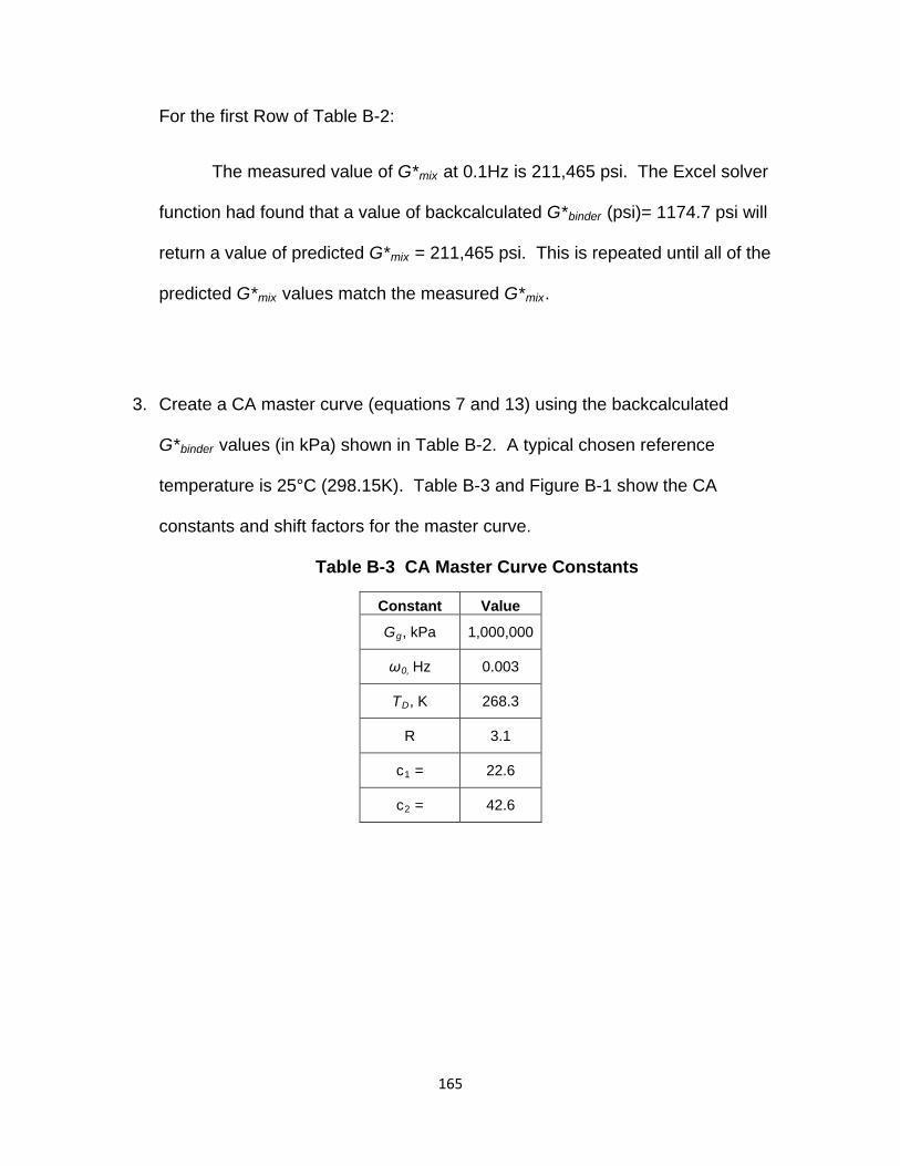
For the first Row of Table B-2:
The measured value of G*mix at 0.1Hz is 211,465 psi. The Excel solver
function had found that a value of backcalculated G*binder (psi)= 1174.7 psi will
return a value of predicted G*mix = 211,465 psi. This is repeated until all of the
predicted G*mix values match the measured G*mix.
3. Create a CA master curve (equations 7 and 13) using the backcalculated
G*binder values (in kPa) shown in Table B-2. A typical chosen reference
temperature is 25°C (298.15K). Table B-3 and Figure B-1 show the CA
constants and shift factors for the master curve.
Table B-3 CA Master Curve Constants
Constant Value
Gg, kPa 1,000,000
ω0, Hz 0.003
TD, K 268.3
R 3.1
c1 = 22.6
c2 = 42.6
165

Figure B-1 Kaeble Shift Factors
4. Additional temperatures of G*binder and δbinder can be calculated using the
constants shown in Table B-3. For example, to determine the backcalculated
binder properties at 64°C (337.15K) and 1.59 Hz (typical DSR frequency) use the
following steps:
a. Calculate the shift factor for 64°C:
659.43.26815.2986.42
3.26815.2983.2682.3376.42
3.2682.3376.22)64log( −=
−+−
−−+
−−=rtoshiftfacto
-5.0
-4.0
-3.0
-2.0
-1.0
0.0
1.0
20 30 40 50 60
log
shift
fact
or
Temperature, °C
166

b. Calculate the reduced frequency:
000348.010 ))659.4()59.1(log( == −+rFreq
c. Use equations 7 and 11 to calculate G*binder and δbinder:
( ) kPaeGG
R
R
g 7.690000348.
003.10611*2log1.3
1.32log2log2log
0 =
+=
+=
−−
ωωω
°=
+
=
+
= 7.53
003.0000348.1
90
1
90)(41.3
2log2log
0
R
ωω
ωδ
167

Appendix C
Figure C-1 Virgin Torsion G*mix Results @ 20°C
Figure C-2 Virgin Torsion G*mix Results @ 30°C
-
500
1,000
1,500
2,000
2,500
3,000
3,500
0.01 0.02 0.05 0.10 0.22 0.46 1.00 2.15 4.64 10.00
G* m
ix, M
Pa
Frequency, HzPG 64-22 -4 PG 64-22 -8 PG 76-22 -4 PG 76-22 -8
-
500
1,000
1,500
2,000
2,500
3,000
3,500
0.01 0.02 0.05 0.10 0.22 0.46 1.00 2.15 4.64 10.00
G* m
ix, M
Pa
Frequency, Hz
PG 64-22 -4 PG 64-22 -8 PG 76-22 -4 PG 76-22 -8
168
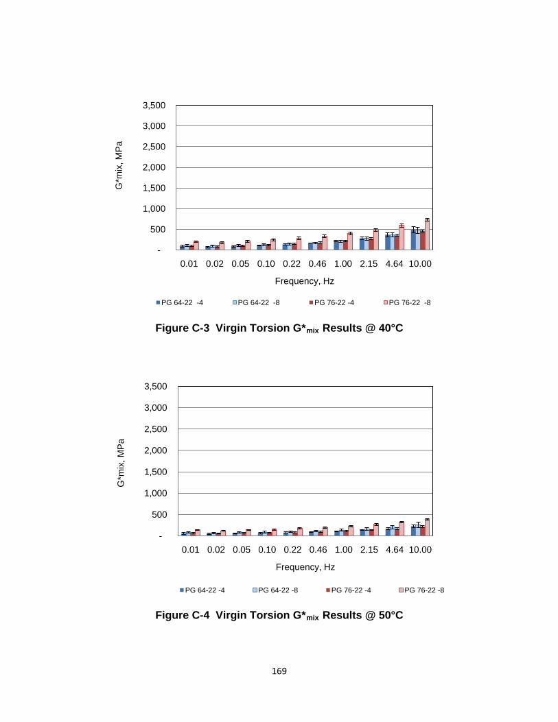
Figure C-3 Virgin Torsion G*mix Results @ 40°C
Figure C-4 Virgin Torsion G*mix Results @ 50°C
-
500
1,000
1,500
2,000
2,500
3,000
3,500
0.01 0.02 0.05 0.10 0.22 0.46 1.00 2.15 4.64 10.00
G*m
ix, M
Pa
Frequency, Hz
PG 64-22 -4 PG 64-22 -8 PG 76-22 -4 PG 76-22 -8
-
500
1,000
1,500
2,000
2,500
3,000
3,500
0.01 0.02 0.05 0.10 0.22 0.46 1.00 2.15 4.64 10.00
G*m
ix, M
Pa
Frequency, Hz
PG 64-22 -4 PG 64-22 -8 PG 76-22 -4 PG 76-22 -8
169

Figure C-5 Virgin Torsion G*mix Results @ 60°C
Figure C-6 Virgin Torsion δmix Results @ 20°C
-
500
1,000
1,500
2,000
2,500
3,000
3,500
0.01 0.02 0.05 0.10 0.22 0.46 1.00 2.15 4.64 10.00
G*m
ix, M
Pa
Frequency, Hz
PG 64-22 -4 PG 64-22 -8 PG 76-22 -4 PG 76-22 -8
-
5.0
10.0
15.0
20.0
25.0
30.0
35.0
40.0
45.0
0.01 0.02 0.05 0.10 0.22 0.46 1.00 2.15 4.64 10.00
δ mix, d
egre
es
Frequency, HzPG 64-22 -4 PG 64-22 -8 PG 76-22 -4 PG 76-22 -8
170

Figure C-7 Virgin Torsion δmix Results @ 30°C
Figure C-8 Virgin Torsion δmix Results @ 40°C
-
5.0
10.0
15.0
20.0
25.0
30.0
35.0
40.0
45.0
0.01 0.02 0.05 0.10 0.22 0.46 1.00 2.15 4.64 10.00
δ mix, d
egre
es
Frequency, HzPG 64-22 -4 PG 64-22 -8 PG 76-22 -4 PG 76-22 -8
-
5.0
10.0
15.0
20.0
25.0
30.0
35.0
40.0
45.0
0.01 0.02 0.05 0.10 0.22 0.46 1.00 2.15 4.64 10.00
δ mix, d
egre
es
Frequency, HzPG 64-22 -4 PG 64-22 -8 PG 76-22 -4 PG 76-22 -8
171

Figure C-9 Virgin Torsion δmix Results @ 50°C
Figure C-10 Virgin Torsion δmix Results @ 60°C
-
5.0
10.0
15.0
20.0
25.0
30.0
35.0
40.0
45.0
0.01 0.02 0.05 0.10 0.22 0.46 1.00 2.15 4.64 10.00
δ mix, d
egre
es
Frequency, HzPG 64-22 -4 PG 64-22 -8 PG 76-22 -4 PG 76-22 -8
-
5.0
10.0
15.0
20.0
25.0
30.0
35.0
40.0
45.0
0.01 0.02 0.05 0.10 0.22 0.46 1.00 2.15 4.64 10.00
δ mix, d
egre
es
Frequency, Hz
PG 64-22 -4 PG 64-22 -8 PG 76-22 -4 PG 76-22 -8
172

Figure C-11 RAP Torsion G*mix Results @ 20°C
Figure C-12 RAP Torsion G*mix Results @ 30°C
-
1,000
2,000
3,000
4,000
5,000
6,000
0.01 0.02 0.05 0.10 0.22 0.46 1.00 2.15 4.64 10.00
G* m
ix, m
Pa
Frequency, HzRAP 1 RAP 2 RAP 3 RAP 4 RAP 5
-
1,000
2,000
3,000
4,000
5,000
6,000
0.01 0.02 0.05 0.10 0.22 0.46 1.00 2.15 4.64 10.00
G*m
ix, M
Pa
Frequency, Hz
RAP 1 RAP 2 RAP 3 RAP 4 RAP 5
173

Figure C-13 RAP Torsion G*mix Results @ 40°C
Figure C-14 RAP Torsion G*mix Results @ 50°C
-
1,000
2,000
3,000
4,000
5,000
6,000
0.01 0.02 0.05 0.10 0.22 0.46 1.00 2.15 4.64 10.00
G*m
ix, M
Pa
Frequency, Hz
RAP 1 RAP 2 RAP 3 RAP 4 RAP 5
-
1,000
2,000
3,000
4,000
5,000
6,000
0.01 0.02 0.05 0.10 0.22 0.46 1.00 2.15 4.64 10.00
G*m
ix, M
Pa
Frequency, Hz
RAP 1 RAP 2 RAP 3 RAP 4 RAP 5
174

Figure C-15 RAP Torsion G*mix Results @ 60°C
Figure C-16 RAP Torsion δmix Results @ 20°C
-
1,000
2,000
3,000
4,000
5,000
6,000
0.01 0.02 0.05 0.10 0.22 0.46 1.00 2.15 4.64 10.00
G*m
ix, M
Pa
Frequency, Hz
RAP 1 RAP 2 RAP 3 RAP 4 RAP 5
0.0
5.0
10.0
15.0
20.0
25.0
30.0
35.0
0.01 0.02 0.05 0.10 0.22 0.46 1.00 2.15 4.64 10.00
δ mix, d
egre
es
Frequency, HzRAP 1 RAP 2 RAP 3 rAP 4 RAP 5
175
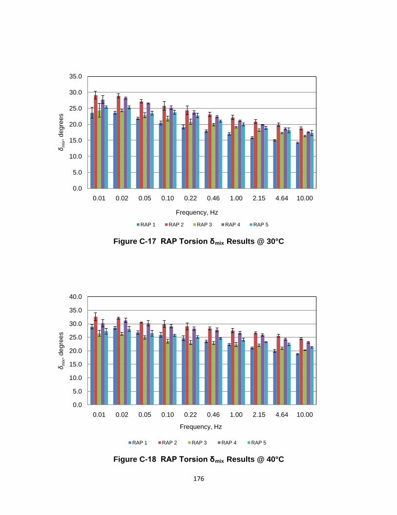
Figure C-17 RAP Torsion δmix Results @ 30°C
Figure C-18 RAP Torsion δmix Results @ 40°C
0.0
5.0
10.0
15.0
20.0
25.0
30.0
35.0
0.01 0.02 0.05 0.10 0.22 0.46 1.00 2.15 4.64 10.00
δ mix, d
egre
es
RAP 1 RAP 2 RAP 3 RAP 4 RAP 5
Frequency, Hz
0.0
5.0
10.0
15.0
20.0
25.0
30.0
35.0
40.0
0.01 0.02 0.05 0.10 0.22 0.46 1.00 2.15 4.64 10.00
δ mix, d
egre
es
RAP 1 RAP 2 RAP 3 RAP 4 RAP 5
Frequency, Hz
176

Figure C-19 RAPTorsion δmix Results @ 50°C
Figure C-20 RAP Torsion δmix Results @ 60°C
0.0
5.0
10.0
15.0
20.0
25.0
30.0
35.0
0.01 0.02 0.05 0.10 0.22 0.46 1.00 2.15 4.64 10.00
δ mix, d
egre
es
RAP 1 RAP 2 RAP 3 RAP 4 RAP 5
Frequency, Hz
0.0
5.0
10.0
15.0
20.0
25.0
30.0
35.0
40.0
0.01 0.02 0.05 0.10 0.22 0.46 1.00 2.15 4.64 10.00
δ mix, d
egre
es
RAP 1 RAP 2 RAP 3 RAP 4 RAP 5
Frequency, Hz
177

Appendix D
Figure D-1 RAP 1 Calculation Comparison for Original and Revised Hirsch
Figure D-2 RAP 2 Calculation Comparison for Original and Revised Hirsch
R² = 0.9511
R² = 0.9208
0.0E+00
5.0E+02
1.0E+03
1.5E+03
2.0E+03
2.5E+03
3.0E+03
3.5E+03
4.0E+03
0.0E+00 1.0E+03 2.0E+03 3.0E+03 4.0E+03
Cal
cula
ted
G* m
ix, M
Pa
Tested G*mix, MPaOriginal Model Revised Model Line of Equality 95% CI Orig 95% CI Rev
R² = 0.9306
R² = 0.9310
0.0E+00
5.0E+02
1.0E+03
1.5E+03
2.0E+03
2.5E+03
3.0E+03
3.5E+03
0.0E+00 5.0E+02 1.0E+03 1.5E+03 2.0E+03 2.5E+03 3.0E+03 3.5E+03
Cal
cula
ted
G* m
ix, M
Pa
Tested G*mix, MPaOriginal Hirsch Revised Hirsch 95% CI Orig 95% CI Rev
178
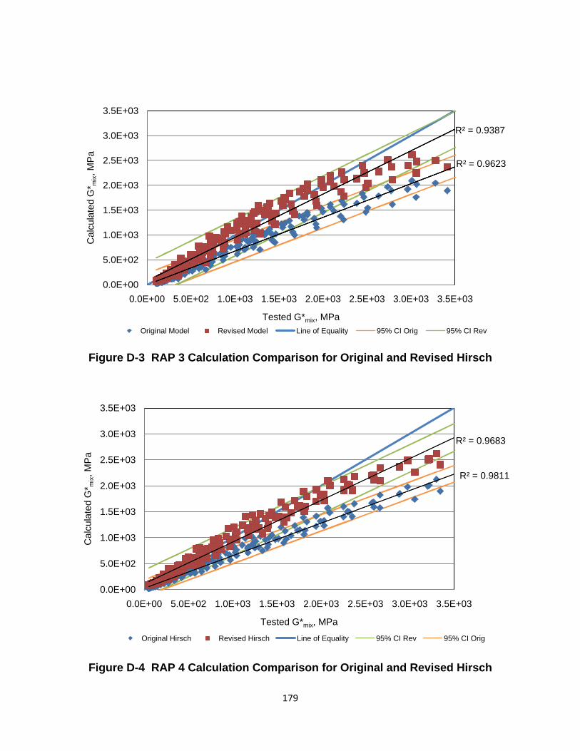
Figure D-3 RAP 3 Calculation Comparison for Original and Revised Hirsch
Figure D-4 RAP 4 Calculation Comparison for Original and Revised Hirsch
R² = 0.9623
R² = 0.9387
0.0E+00
5.0E+02
1.0E+03
1.5E+03
2.0E+03
2.5E+03
3.0E+03
3.5E+03
0.0E+00 5.0E+02 1.0E+03 1.5E+03 2.0E+03 2.5E+03 3.0E+03 3.5E+03
Cal
cula
ted
G* m
ix, M
Pa
Tested G*mix, MPaOriginal Model Revised Model Line of Equality 95% CI Orig 95% CI Rev
R² = 0.9811
R² = 0.9683
0.0E+00
5.0E+02
1.0E+03
1.5E+03
2.0E+03
2.5E+03
3.0E+03
3.5E+03
0.0E+00 5.0E+02 1.0E+03 1.5E+03 2.0E+03 2.5E+03 3.0E+03 3.5E+03
Cal
cula
ted
G* m
ix, M
Pa
Tested G*mix, MPa
Original Hirsch Revised Hirsch Line of Equality 95% CI Rev 95% CI Orig
179

Figure D-5 RAP 5 Calculation Comparison for Original and Revised Hirsch
R² = 0.9406
R² = 0.9388
0.0E+00
5.0E+02
1.0E+03
1.5E+03
2.0E+03
2.5E+03
3.0E+03
3.5E+03
0.0E+00 5.0E+02 1.0E+03 1.5E+03 2.0E+03 2.5E+03 3.0E+03 3.5E+03
Cal
cula
ted
G* m
ix, M
Pa
Tested G*mix, MPa
Original Hirsch Revised Hirsch Line of Equality 95% CI Orig 95% CI Rev
180
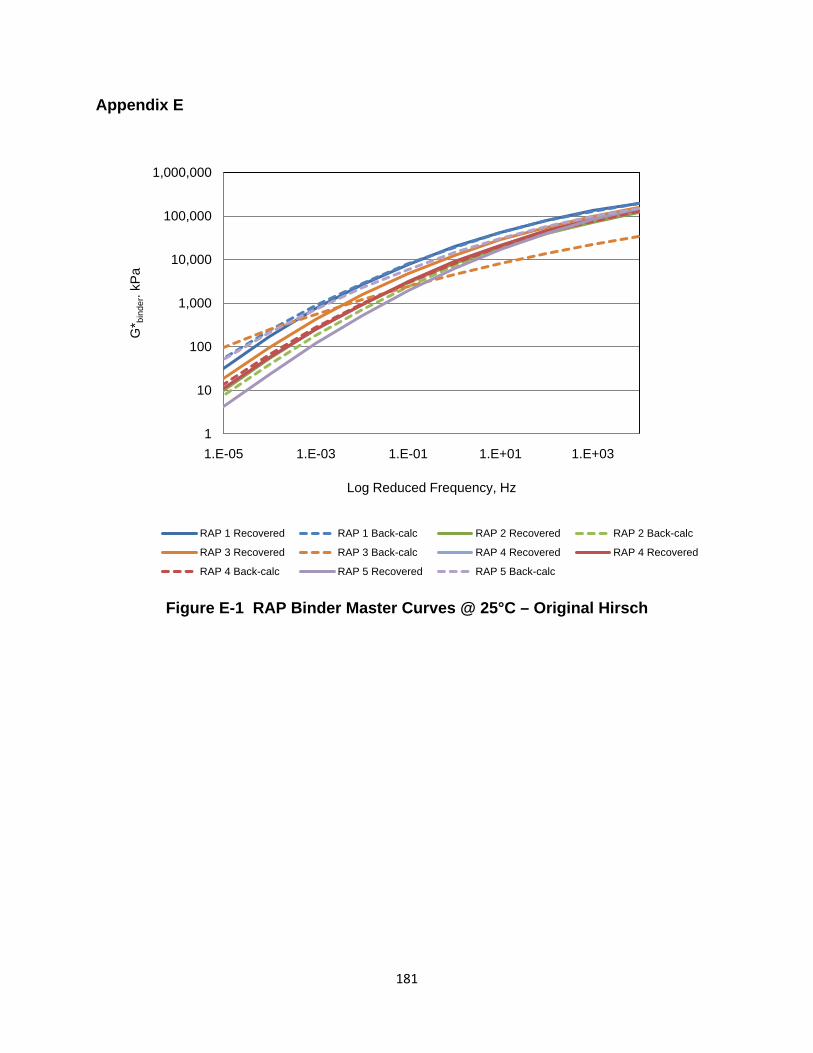
Appendix E
Figure E-1 RAP Binder Master Curves @ 25°C – Original Hirsch
1
10
100
1,000
10,000
100,000
1,000,000
1.E-05 1.E-03 1.E-01 1.E+01 1.E+03
G* b
inde
r. kP
a
Log Reduced Frequency, Hz
RAP 1 Recovered RAP 1 Back-calc RAP 2 Recovered RAP 2 Back-calc
RAP 3 Recovered RAP 3 Back-calc RAP 4 Recovered RAP 4 Recovered
RAP 4 Back-calc RAP 5 Recovered RAP 5 Back-calc
181

Figure E-2 RAP Binder Master Curves @ 25°C – Revised Hirsch
1
10
100
1,000
10,000
100,000
1,000,000
1.E-05 1.E-03 1.E-01 1.E+01 1.E+03
G* b
inde
r. kP
a
Log Reduced Frequency, Hz
RAP 1 Recovered RAP 1 Back-calc RAP 2 Recovered RAP 2 Back-calc
RAP 3 Recovered RAP 3 Back-calc RAP 4 Recovered RAP 4 Back-calc
RAP 5 Recovered RAP 5 Back-calc
182

Figure E-3 High Temp Backcalculated G*binder Results- RAP 1
Figure E-4 Intermediate Temp Backcalculated G*binder Results- RAP 1
0.00
10.00
20.00
30.00
40.00
50.00
60.00
70.00
80.00
90.00
94 100
Back
-Cal
cula
ted
G* b
inde
r, kP
a
Temperature, °C
Tested Binder
OH
RH
0
2000
4000
6000
8000
10000
12000
14000
16000
18000
37 40
Back
-Cal
cula
ted
G* b
inde
r, kP
a
Temperature, °C
Tested Binder
OH
RH
183
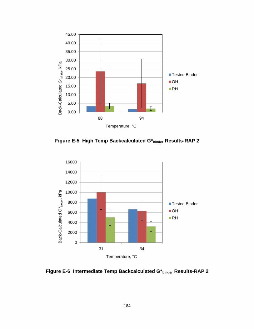
Figure E-5 High Temp Backcalculated G*binder Results-RAP 2
Figure E-6 Intermediate Temp Backcalculated G*binder Results-RAP 2
0.00
5.00
10.00
15.00
20.00
25.00
30.00
35.00
40.00
45.00
88 94
Back
-Cal
cula
ted
G* b
inde
r, kP
a
Temperature, °C
Tested Binder
OH
RH
0
2000
4000
6000
8000
10000
12000
14000
16000
31 34
Back
-Cal
cula
ted
G* b
inde
r, kP
a
Temperature, °C
Tested Binder
OH
RH
184

Figure E-7 High Temp Backcalculated G*binder Results-RAP 3
Figure E-8 Intermediate Temp Backcalculated G*binder Results- RAP 3
0.00
10.00
20.00
30.00
40.00
50.00
60.00
70.00
80.00
94 100
Back
-Cal
cula
ted
G* b
inde
r, kP
a
Temperature, °C
Tested Binder
OH
RH
0
2000
4000
6000
8000
10000
12000
14000
16000
18000
31 34
Back
-Cal
cula
ted
G* b
inde
r, kP
a
Temperature, °C
Tested Binder
OH
RH
185

Figure E-9 High Temp Backcalculated G*binder Results-RAP 4
Figure E-10 Intermediate Temp Backcalculated G*binder Results-RAP 4
0
5
10
15
20
25
30
35
82 88
Back
-Cal
cula
ted
G* b
inde
r, kP
a
Temperature, °C
Tested Binder
OH
RH
0
5000
10000
15000
20000
25000
28 31
Back
-Cal
cula
ted
G* b
inde
r, kP
a
Temperature, °C
Tested Binder
OH
RH
186

Figure E-11 High-temperature Backcalculated G*binder Results-RAP 5
Figure E-12 Intermediate Temp Backcalculated G*binder Results- RAP 5
0.00
20.00
40.00
60.00
80.00
100.00
120.00
140.00
160.00
82 88
Back
-Cal
cula
ted
G* b
inde
r, kP
a
Temperature, °C
Tested Binder
OH
RH
0
50000
100000
150000
200000
250000
25 28
Back
-Cal
cula
ted
G* b
inde
r, kP
a
Temperature, °C
Tested Binder
OH
RH
187

Figure E-13 High Temp Backcalculated δbinder Results- RAP 1
Figure E-14 Intermediate Temp Backcalculated δbinder Results-RAP 1
0.0
10.0
20.0
30.0
40.0
50.0
60.0
70.0
80.0
90.0
94 100
Back
-Cal
cula
tedδ b
inde
r, °
Temperature, °C
Tested Binder
OH
RH
0
5
10
15
20
25
30
35
40
45
50
37 40
Back
-Cal
cula
ted
δ bin
der,
°
Temperature, °C
Tested Binder
OH
RH
188

Figure E-15 High Temp Backcalculated δbinder Results-RAP 2
Figure E-16 Intermediate Temp Backcalculated δbinder Results-RAP 2
0
10
20
30
40
50
60
70
80
90
88 94
Back
-Cal
cula
tedδ b
inde
r, °
Temperature, °C
Tested Binder
OH
RH
0
5
10
15
20
25
30
35
40
45
50
31 34
Back
-Cal
cula
ted
δ bin
der,
°
Temperature, °C
Tested Binder
OH
RH
189

Figure E-17 High Temp Backcalculated δbinder Results-RAP 3
Figure E-18 Intermediate Temp Backcalculated δbinder Results-RAP 3
0
10
20
30
40
50
60
70
80
90
94 100
Back
-Cal
cula
tedδ b
inde
r, °
Temperature, °C
Tested Binder
OH
RH
0
5
10
15
20
25
30
35
40
45
31 34
Back
-Cal
cula
ted
δ bin
der,
°
Temperature, °C
Tested Binder
OH
RH
190

Figure E-19 High Temp Backcalculated δbinder Result-RAP 4
Figure E-20 Intermediate Temp Backcalculated δbinder Results-RAP 4
0
10
20
30
40
50
60
70
80
90
82 88
Back
-Cal
cula
tedδ b
inde
r, °
Temperature, °C
Tested Binder
OH
RH
0
5
10
15
20
25
30
35
40
45
28 31
Back
-Cal
cula
ted
δ bin
der,
°
Temperature, °C
Tested Binder
OH
RH
191

Figure E-21 High Temp Backcalculated δbinder Results-RAP 5
Figure E-22 Intermediate Temp Backcalculated δbinder Results-RAP 5
0
10
20
30
40
50
60
70
80
90
82 88
Back
-Cal
cula
tedδ b
inde
r, °
Temperature, °C
Tested Binder
OH
RH
0
5
10
15
20
25
30
35
40
45
25 28
Back
-Cal
cula
ted
δ bin
der,
°
Temperature, °C
Tested Binder
OH
RH
192

Figure E-23 Backcalculated Tcrit-RAP 1
Figure E-24 Backcalculated Tcrit -RAP 2
0
20
40
60
80
100
120
140
160
180
200
Tcrit, High Tcrit, Int
Tem
pera
ture
, °C
Binder
Original Hirsch
Revised Hirsch
0
20
40
60
80
100
120
140
160
Tcrit, High Tcrit, Int
Tem
pera
ture
, °C
Binder
Original Hirsch
Revised Hirsch
193

Figure E-25 Backcalculated Tcrit -RAP 3
Figure E-26 Backcalculated Tcrit -RAP 4
0
20
40
60
80
100
120
140
160
180
Tcrit, High Tcrit, Int
Tem
pera
ture
, °C
Binder
Original Hirsch
Revised Hirsch
0
20
40
60
80
100
120
140
Tcrit, High Tcrit, Int
Tem
pera
ture
, °C
Binder
Original Hirsch
Revised Hirsch
194

Figure E-27 Backcalculated Tcrit -RAP 5
0.0
20.0
40.0
60.0
80.0
100.0
120.0
140.0
160.0
180.0
200.0
Tcrit, High Tcrit, Int
Tem
pera
ture
, °C
Binder
Original Hirsch
Revised Hirsch
195

Appendix F
Figure F-1 PG 64-22 Laboratory Blend Master Curves for OH Model – RAP 2
Figure F-2 PG 64-22 Laboratory Blend Master Curves for RH Model – RAP 2
0.01
0.10
1.00
10.00
100.00
1,000.00
10,000.00
100,000.00
1,000,000.00
1.E-06 1.E-04 1.E-02 1.E+00 1.E+02 1.E+04 1.E+06
|G* b
inde
r|, k
Pa
Log Reduced Frequency, Hz
PG 64-22 OH 20% OH 35% OH 50% 100% RAP 2
0.01
0.10
1.00
10.00
100.00
1,000.00
10,000.00
100,000.00
1,000,000.00
1.E-06 1.E-04 1.E-02 1.E+00 1.E+02 1.E+04 1.E+06
|G* b
inde
r|, k
Pa
Log Reduced Frequency, Hz
PG 64-22 RH 20% RH 35% RH 50% 100% RAP 2
196

Figure F-3 PG 76-22 Laboratory Blend Master Curves for OH Model – RAP 2
Figure F-4 PG 76-22 Laboratory Blend Master Curves for RH Model – RAP 2
0.01
0.10
1.00
10.00
100.00
1,000.00
10,000.00
100,000.00
1,000,000.00
1.E-06 1.E-04 1.E-02 1.E+00 1.E+02 1.E+04 1.E+06
|G* b
inde
r|, k
Pa
Log Reduced Frequency, Hz
PG 76-22 OH 20% OH 35% OH 50% 100% RAP 2
0.01
0.10
1.00
10.00
100.00
1,000.00
10,000.00
100,000.00
1,000,000.00
1.E-06 1.E-04 1.E-02 1.E+00 1.E+02 1.E+04 1.E+06
|G* b
inde
r|, k
Pa
Log Reduced Frequency, Hz
PG 76-22 RH 20 RH 35% RH 50% 100% RAP 2
197

Figure F-5 PG 64-22 Laboratory Blend Master Curves for OH Model – RAP 3
Figure F-6 PG 64-22 Laboratory Blend Master Curves for RH Model – RAP 3
0.01
0.10
1.00
10.00
100.00
1,000.00
10,000.00
100,000.00
1,000,000.00
1.E-06 1.E-04 1.E-02 1.E+00 1.E+02 1.E+04 1.E+06
|G* b
inde
r|, k
Pa
Log Reduced Frequency, Hz
PG 64-22 OH 20% OH 35% OH 50% 100% RAP 3
0.01
0.10
1.00
10.00
100.00
1,000.00
10,000.00
100,000.00
1,000,000.00
1.E-06 1.E-04 1.E-02 1.E+00 1.E+02 1.E+04 1.E+06
|G* b
inde
r|, k
Pa
Reduced Frequency, Hz
PG 64-22 RH 20% RH 35% RH 50% 100% RAP 3
198

Figure F-7 PG 76-22 Laboratory Blend Master Curves for OH Model – RAP 3
Figure F-8 PG 76-22 Laboratory Blend Master Curves for RH Model – RAP 3
0.01
0.10
1.00
10.00
100.00
1,000.00
10,000.00
100,000.00
1,000,000.00
1.E-06 1.E-04 1.E-02 1.E+00 1.E+02 1.E+04 1.E+06
|G* b
inde
r|, k
Pa
Log Reduced Frequency, Hz
PG 76-22 OH 20% OH 35% OH 50% 100% RAP 3
0.01
0.10
1.00
10.00
100.00
1,000.00
10,000.00
100,000.00
1,000,000.00
1.E-06 1.E-04 1.E-02 1.E+00 1.E+02 1.E+04 1.E+06
|G* b
inde
r|, k
Pa
Log Reduced Frequency, Hz
PG 76-22 RH 20 RH 35% RH 50% 100% RAP 3
199

Figure F-9 PG 64-22 Laboratory Blend Master Curves for OH Model – RAP 5
Figure F-10 PG 64-22 Laboratory Blend Master Curves for RH Model – RAP 5
0.01
0.10
1.00
10.00
100.00
1,000.00
10,000.00
100,000.00
1,000,000.00
1.E-06 1.E-04 1.E-02 1.E+00 1.E+02 1.E+04 1.E+06
|G* b
inde
r|, k
Pa
Log Reduced Frequency, Hz
PG 64-22 OH 20% OH 35% OH 50% 100% RAP 5
0.01
0.10
1.00
10.00
100.00
1,000.00
10,000.00
100,000.00
1,000,000.00
1.E-06 1.E-04 1.E-02 1.E+00 1.E+02 1.E+04 1.E+06
|G* b
inde
r|, k
Pa
Log Reduced Frequency, Hz
PG 64-22 100% RAP 5 RH 20% RH 35% RH 50%
200

Figure F-11 PG 76-22 Laboratory Blend Master Curves for OH Model – RAP 5
Figure F-12 PG 76-22 Laboratory Blend Master Curves for RH Model – RAP 5
0.01
0.10
1.00
10.00
100.00
1,000.00
10,000.00
100,000.00
1,000,000.00
1.E-06 1.E-04 1.E-02 1.E+00 1.E+02 1.E+04 1.E+06
|G* b
inde
r|, k
Pa
Log Reduced Frequency, HzPG 76-22 OH 20% OH 35% OH 50% 100% RAP 5
0.01
0.10
1.00
10.00
100.00
1,000.00
10,000.00
100,000.00
1,000,000.00
1.E-06 1.E-04 1.E-02 1.E+00 1.E+02 1.E+04 1.E+06
|G* b
inde
r|, k
Pa
Log Reduced Frequency, Hz
PG 76-22 100% RAP 5 RH 20 RH 35% RH 50%
201
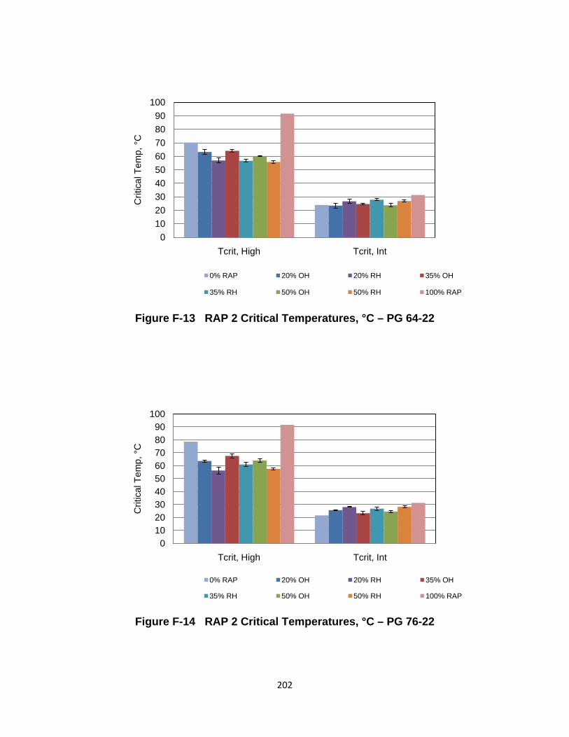
Figure F-13 RAP 2 Critical Temperatures, °C – PG 64-22
Figure F-14 RAP 2 Critical Temperatures, °C – PG 76-22
0102030405060708090
100
Tcrit, High Tcrit, Int
Crit
ical
Tem
p, °
C
0% RAP 20% OH 20% RH 35% OH
35% RH 50% OH 50% RH 100% RAP
0102030405060708090
100
Tcrit, High Tcrit, Int
Crit
ical
Tem
p, °
C
0% RAP 20% OH 20% RH 35% OH
35% RH 50% OH 50% RH 100% RAP
202

Figure F-15 RAP 3 Critical Temperatures, °C – PG 64-22
Figure F-16 RAP 3 Critical Temperatures, °C – PG 76-22
0102030405060708090
100
Tcrit, High Tcrit, Int
Crit
ical
Tem
ps, °
C
0% RAP 20% OH 20% RH 35% OH
35% RH 50% OH 50% RH 100% RAP
0102030405060708090
100
Tcrit, High Tcrit, Int
Crit
ical
Tem
ps, °
C
0% RAP 20% OH 20% RH 35% OH
35% RH 50% OH 50% RH 100% RAP
203

Figure F-17 RAP 5 Critical Temperatures, °C – PG 64-22
Figure F-18 RAP 5 Critical Temperatures, °C – PG 76-22
0102030405060708090
100
Tcrit, High Tcrit, Int
Crit
ical
Tem
ps, °
C
0% RAP 20% OH 20% RH 35% OH
35% RH 50% OH 50% RH 100% RAP
0102030405060708090
100
Tcrit, High Tcrit, Int
Crit
ical
Tem
ps, °
C
0% RAP 20% OH 20% RH 35% OH
35% RH 50% OH 50% RH 100% RAP
204

Figure F-19 PG 64-22 Blending Chart – RAP 2
Figure F-20 PG 76-22 Blending Chart – RAP 2
0.010.020.030.040.050.060.070.080.090.0
100.0
0 20 40 60 80 100
Crit
ical
Tem
p, °
C
% RAP
PG 64-22 high PG 64-22 int original HIrschRevised Hirsch original Hirsch int Revised Hirsch Int
0.010.020.030.040.050.060.070.080.090.0
100.0
0 20 40 60 80 100
Crit
ical
Tem
p, °
C
% RAP
PG 76-22 HIgh PG 76-22 Int original HIrschRevised Hirsch original Hirsch int Revised Hirsch Int
205

Figure F-21: PG 64-22 Blending Chart – RAP 3
Figure F-22 PG 76-22 Blending Chart – RAP 3
0.010.020.030.040.050.060.070.080.090.0
100.0
0 20 40 60 80 100
Crit
ical
Tem
p, °
C
% RAP
PG 64-22 high PG 64-22 int original HIrsch
Revised Hirsch original Hirsch int Revised Hirsch Int
0.010.020.030.040.050.060.070.080.090.0
100.0
0 20 40 60 80 100
Crit
ical
Tem
p, °
C
% RAP
PG 76-22 PG 76-22 int original HIrsch
Revised Hirsch original Hirsch int Revised Hirsch Int
206

Figure F-23 PG 64-22 Blending Chart – RAP 5
Figure F-24 PG 76-22 Blending Chart – RAP 5
0.010.020.030.040.050.060.070.080.090.0
0 20 40 60 80 100
Crit
ical
Tem
p, °
C
% RAP
PG 64-22 high PG 64-22 int original HIrschRevised Hirsch original Hirsch int Revised Hirsch Int
0.0
10.0
20.0
30.0
40.0
50.0
60.0
70.0
80.0
90.0
0 20 40 60 80 100
Crit
ical
Tem
p, °
C
% RAP
PG 76-22 PG 76-22 Int original HIrschRevised Hirsch original Hirsch int Revised Hirsch Int
207

Figure F-25 Plant Mix A Critical Temperatures, °C
Figure F-26 Plant Mix B Critical Temperatures, °C
0
10
20
30
40
50
60
70
80
90
100
Tcrit, High Tcrit, Int
Crit
ical
Tem
p, °
C
OH RH Recovered BInder Blending Chart
0102030405060708090
100
Tcrit, High Tcrit, Int
Crit
ical
Tem
p, °
C
OH RH Recovered Binder Blending Chart
208

Figure F-27 Plant Mix C Critical Temperatures, °C
Figure F-28 Plant Mix D Critical Temperatures, °C
0102030405060708090
100
Tcrit, High Tcrit, Int
Crit
ical
Tem
p, °
C
OH RH Blending Chart
0102030405060708090
100
Tcrit, High Tcrit, Int
Crit
ical
Tem
p, °
C
OH RH Recovered Binder Blending Chart
209

Figure F-29 Plant Mix E Critical Temperatures, °C
0
10
20
30
40
50
60
70
80
90
100
Tcrit, High Tcrit, Int
Crit
ical
Tem
p, °
C
OH RH Recovered Binder Blending Chart
210