evaluation of a sontek acoustic doppler meter
TRANSCRIPT

EVALUATION OF A SONTEK ACOUSTIC DOPPLER METER
by
Lynn Groundwater
BioResource and Agricultural Engineering
BioResource and Agricultural Engineering Department
California Polytechnic State University
San Luis Obispo
June 2011

ii
SIGNATURE PAGE
TITLE : Evaluation of a SonTek Acoustic Doppler Flow Meter AUTHOR : Lynn Groundwater DATE SUBMITTED : June 10, 2011
Stuart Styles Senior Project Advisor Signature
Richard A. Cavaletto
Date
Department Head Signature
Date

iii
ABSTRACT
The Tehama-Colusa Canal Authority (TCCA) has been using SonTek Doppler flow meters at approximately 30 installations for about 3 years. TCCA is located in northern California with its headquarters in Willows. The Cal Poly ITRC compared the accuracy of the volumetric readings from the new Doppler flow meters to the venturi meters that were installed by the US Bureau of Reclamation (USBR) and were the historical standard for flow measurement for TCCA. Delano-Earlimart Irrigation District (DEID) installed the SonTek into 2 of its laterals. DEID is located in Central California north of Bakersfield. TCCA and DEID have opted to move away from the existing technology for a variety of reasons, especially concerning access requirements for an enclosed space. TCCA has opted to use the Doppler meter as the replacement. USBR has proposed using one standard deviation for the evaluation of the minimum number of data points to calibrate a site. In past studies, ITRC has used the R-Squared statistic to set the minimum number of data points. This senior project evaluates the technique used to report calibration of a meter.
iv
DISCLAIMER STATEMENT
The university makes it clear that the information forwarded herewith is a project resulting from a class assignment and has been graded and accepted only as a fulfillment of a course requirement. Acceptance by the university does not imply technical accuracy or reliability. Any use of the information in this report is made by the user(s) at his/her own risk, which may include catastrophic failure of the device or infringement of patent or copyright laws. Therefore, the recipient and/or user of the information contained in this report agrees to indemnify, defend and save harmless the State its officers, agents and employees from any and all claims and losses accruing or resulting to any person, firm, or corporation who may be injured or damaged as a result of the use of this report.

v
Table of Contents
Page
SIGNATURE PAGE .......................................................................................................... ii
ABSTRACT ....................................................................................................................... iii
DISCLAIMER STATEMENT .......................................................................................... iv
LIST OF FIGURES .......................................................................................................... vii
LIST OF TABLES ............................................................................................................. ix
INTRODUCTION .............................................................................................................. 1
LITERATURE REVIEW ................................................................................................... 2
Flow Measurement....................................................................................................................... 2
Accuracy ...................................................................................................................................... 3
Statistical Analysis ....................................................................................................................... 7
PROCEDURES AND METHODS..................................................................................... 8
Tehama-Colusa Canal Authority ................................................................................................. 8
SonTek Installation/Calibration. .............................................................................................. 9
Delano-Earlimart Irrigation District ........................................................................................... 11
SonTek Installation at Lateral 56W. ...................................................................................... 11
SonTek Installation Lateral 40W. .......................................................................................... 12
Measurement Procedure ............................................................................................................. 13
Statistical Method and Data Processing ..................................................................................... 24
RESULTS ......................................................................................................................... 30
DISCUSSION ................................................................................................................... 34
Data Comparison ....................................................................................................................... 34
Statistical Calibration Discussion .............................................................................................. 35
RECOMMENDATIONS .................................................................................................. 40
REFERENCES ................................................................................................................. 41
APPENDIX A ................................................................................................................... 42
How Project Meets Requirements for the BRAE Major ............................................................ 42
APPENDIX B ................................................................................................................... 46
Calibration Sheets ...................................................................................................................... 46
APPENDIX C ................................................................................................................... 47

vi
TCCA Venturi Calibration ......................................................................................................... 47

vii
LIST OF FIGURES
Page
Figure 1 Flowmeters (U.S., 2001) ...................................................................................... 5 Figure 2 SonTek Argonaut-SW (SonTek/YSI Inc., 2009). ................................................ 6 Figure 3 How the Argonaut-SW works (SonTek/YSI Inc., 2009). .................................... 7 Figure 4 TCCA Venturi Meter ............................................................................................ 9 Figure 5 Installation of SonTek Meter .............................................................................. 10 Figure 6 Schematic of Layout of Lateral 56W SonTek Installation ................................. 12 Figure 8 View Argonaut Icon ........................................................................................... 13 Figure 7 SonTek Argonaut-SW mounting locations – Lateral 40W ................................ 13 Figure 9 View Argonaut Main Screen .............................................................................. 14 Figure 10 View Argonaut Recorder Screen ...................................................................... 14 Figure 11 View Argonaut Display Screen-Connected ...................................................... 15 Figure 12 View Argonaut Recorder Screen- Download Files .......................................... 15 Figure 14 View Argonaut- Session Type.......................................................................... 16 Figure 13 View Argonaut Recorder Screen- Format Files ............................................... 16 Figure 15 View Argonaut- Connect to System ................................................................. 17 Figure 16 View Argonaut- System Settings ..................................................................... 17 Figure 17 View Argonaut-Load Template ........................................................................ 17 Figure 18 View Argonaut- Units ...................................................................................... 18 Figure 19 View Argonaut- Set Time ................................................................................ 18 Figure 20 View Argonaut- Match Computer Time .......................................................... 19 Figure 21 View Argonaut- Data Interval .......................................................................... 19 Figure 22 View Argonaut- Profile Settings ...................................................................... 19 Figure 23 View Argonaut- Coordinate System ................................................................ 20 Figure 24 View Argonaut- Burst Mode ............................................................................ 20 Figure 25 View Argonaut- Channel Geometry ................................................................. 21 Figure 26 View Argonaut- Velocity Calculation .............................................................. 21 Figure 27 View Argonaut- Volume .................................................................................. 22 Figure 28 View Argonaut- Output Type ........................................................................... 22 Figure 29 View Argonaut- Battery ................................................................................... 22 Figure 30 View Argonaut- Summary ............................................................................... 23 Figure 31 View Argonaut- Update System ....................................................................... 23 Figure 32 View Argonaut- Start Deployment ................................................................... 23 Figure 33 View Argonaut- Deployment Finished ............................................................ 24 Figure 34 View Argonaut- Exit ........................................................................................ 24 Figure 35 View Argonaut Icon ......................................................................................... 24 Figure 36 View Argonaut- Main Screen ........................................................................... 25 Figure 37 View Argonaut- Processing Screen .................................................................. 25

viii
Figure 38 View Argonaut- Open File ............................................................................... 25 Figure 39 View Argonaut- Data Information ................................................................... 26 Figure 40 View Argonaut- Processing .............................................................................. 26 Figure 41 View Argonaut- Flow Calculation ................................................................... 27 Figure 42 View Argonaut- Channel Geometery ............................................................... 27 Figure 43 View Argonaut- File ......................................................................................... 27 Figure 44 View Argonaut- Export Data ............................................................................ 28 Figure 45 View Argonaut- Discharge Data ...................................................................... 28 Figure 46 Volume graphs of Lateral 56W (2007-2010) ................................................... 32 Figure 47 Volume graphs of Lateral 40W (2009-2010) ................................................... 33 Figure 48 Venturi line being bled of air ............................................................................ 48 Figure 49 SonTek Flow Display ....................................................................................... 49 Figure 50 Badger Flow Display ........................................................................................ 49

ix
LIST OF TABLES
Page
Table 1 Comparison of TCCA Turnouts after Dopplers Installed (SonTek-Venturi) ................... 30 Table 2 Comparison of DEID Laterals after Dopplers Installed (SonTek-Venturi) ...................... 31 Table 3 Comparison of DEID Turnouts to FWUA Lateral in acre-ft (DEID-FWUA) .................. 34 Table 4 Comparison of DEID Turnouts after SonTeks Installed in acre-ft (DEID-FWUA) ......... 35 Table 5 Comparison of DEID Turnouts after SonTeks Installed in acre-ft (SonTek-FWUA) ...... 35 Table 6 Statistical evaluation of the DEID laterals ........................................................................ 35 Table 7 Summary of the results from Lat 56 and Lat 40 ............................................................... 36 Table 8 Summary of the results from Lat 56 and Lat 40 ............................................................... 37 Table 9 Summary of the results from TCCA laterals .................................................................... 38 Table 10 Summary of the results of TCCA laterals ....................................................................... 39

1
INTRODUCTION
Almost every day there are major headlines in the news regarding the water crisis in California. Even with statewide precipitation and snowpack levels above normal for the 2012 water year many California water users south of the Delta who depend on either the State Water Project or the federal Central Valley Project (CVP) for all or a portion of their water are receiving less than 100 percent of their contracted water allocations. The water from the state and federal water projects is an essential resource for the state’s urban and rural populations, its agricultural industry, as well as many other businesses and industries that depend on a reliable water supply. The demands for water to meet these needs, as well as to meet environmental needs, exceed the available supply. With predictions that global warming will result in rising snow levels, less water would be stored in the snowpack leaving us with less water in storage to carry California through our dry summers. It is important that the water usage is being measured accurately. Water customers do not want to pay for more water than they are receiving. The Tehama-Colusa Canal Authority (TCCA) has been using SonTek Doppler flow meters for at least 3 years. The volume is measured twice: once by the Bureau of Reclamation at the head of the canal and once by TCCA at the laterals. The TCCA volume numbers need to be within 10% of the volume that the volume recorded by the Bureau. TCCA currently uses a venturi with a Badger recording device to measure the flow and the SonTek indexing is adjusted so that the flow rate matches that of the Badger. The Badger is currently used to bill the consumers but TCCA wants to switch over to the SonTeks for billing. TCCA installed the SonTek meters because the recorders on the Badgers are failing and there was no support; the venturi meters have to be bled to get rid of the air; and the SonTeks are an upgrade, more manageable, and easier to maintain. By installing a SonTek, it takes away having to make an entry into a confined space to maintain the meter. The purpose of this project was to check the accuracy of the volumetric readings from the SonTek flow meters compared to the venturi meters that are currently used. Many irrigation districts and other water agencies are moving towards the SonTek Doppler flow meters for these types of sites in order to minimize restrictions associated with confined and enclosed space access. However, the calibration of the units can take some time due to a discussion on the minimum number of data points required to adequately calibrate a field site. For this project data points were collected using the SonTeks and compared to the volume readings of the venturi meters from Tehama-Colusa Canal Authority and Delano Earlimart Irrigation District. Once the data was collected, a statistical analysis was performed in order to determine the minimum number of calibration points required and the relative uncertainty of the device. One standard deviation was used to determine the accuracy of the devices.

2
LITERATURE REVIEW
Public concepts of how to share and manage the finite supplies of water are changing. Increasing competition exists between power, irrigation, municipal, industrial, recreation, aesthetic, and fish and wildlife uses. Within the United States, critical examinations of water use will be based on consumption, perceived waste, population density, and impact on ecological systems and endangered species. Water districts will need to seek ways to extend the use of their supplies of water by the best available technologies. Best management measures and practices without exception depend upon conservation of water. The key to conservation is good water measurement practices (USBR, 2001).
Flow Measurement
As district needs for water increase, plans will be formulated to extend the use of water. Rather than finding and developing new sources, water often can be less expensively provided by conservation and equitable distribution of existing water supplies. Every cubic foot of water recovered as a result of improving water measurement produces more revenue than the same amount obtained from a new source. Better measurement procedures extend the use of water because poor operation and deterioration of the metering equipment usually result in the delivery of excess water to users or unacceptable losses through waste. Beyond the district or supply delivery point, attention to measurement, management, and maintenance will also extend the farmer's water use and help prevent reduced yields and other crop damage caused by over-watering (USBR, 2001). Besides proper billing for water usage, many benefits are derived by upgrading water measurement programs and systems. Although some of the benefits are intangible, they should be considered during system design or when planning a water measurement upgrade. Good water management requires accurate water measurement. Some benefits of improved water measurement are:
• Accurate accounting and good records help allocate equitable shares of water among competitive uses both on and off the farm.
• Good water measurement practices facilitate accurate and equitable distribution of water within a district or farm, resulting in fewer problems and easier operation.
• Accurate water measurement provides the on-farm irrigation decision-maker with the information needed to achieve the best use of the irrigation water applied while typically minimizing negative environmental impacts.
• Installing canal flow measuring structures reduces the need for time-consuming current metering. Without these structures, current metering is frequently needed after making changes of delivery and to make seasonal corrections for changes of boundary resistance caused by weed growths or changes of sectional shape by bank slumping and sediment deposits.
• Instituting accurate and convenient water measurement methods improves the evaluation of seepage losses in unlined channels. Thus, better determinations of the cost benefits of proposed canal and ditch improvements are possible.
• Permanent water measurement devices can also form the basis for future improvements, such as remote flow monitoring and canal operation automation.

3
• Good water measurement and management practice prevents excess runoff and deep percolation, which can damage crops, pollute ground water with chemicals and pesticides, and result in project farm drainage flows containing contaminants.
• Accounting for individual water use combined with pricing policies that penalize excessive use.
Flow is classified into open channel flow and closed conduit flow. Open channel flow conditions occur whenever the flowing stream has a free or unconstrained surface that is open to the atmosphere. Flows in canals or in vented pipelines which are not flowing full are typical examples. The presence of the free water surface prevents transmission of pressure from one end of the conveyance channel to another as in fully flowing pipelines. Thus, in open channels, the only force that can cause flow is the force of gravity on the fluid. As a result, with steady uniform flow under free discharge conditions, a progressive fall or decrease in the water surface elevation always occurs as the flow moves downstream (USBR, 2001). In hydraulics, a pipe is any closed conduit that carries water under pressure. The filled conduit may be square, rectangular, or any other shape, but is usually round. If flow is occurring in a conduit but does not completely fill it, the flow is not considered pipe or closed conduit flow, but is classified as open channel flow (USBR, 2001). Flow occurs in a pipeline when a pressure or head difference exists between ends. The rate or discharge that occurs depends mainly upon (1) the amount of pressure or head difference that exists from the inlet to the outlet; (2) the friction or resistance to flow caused by pipe length, pipe roughness, bends, restrictions, changes in conduit shape and size, and the nature of the fluid flowing; and (3) the cross-sectional area of the pipe (USBR, 2001).
Water is sold and measured in terms of total volume delivered (typically in units of cubic feet or acre feet) over a set period of time period, perhaps for a billing each month. Many flowmeters have built in capability to sum or totalize volume continuously. Thus, the volume consumed is obtained by taking the difference of two sequential monthly readings. To aid irrigation operation and management, most meters provide instantaneous rate of flow or discharge displayed in units such as cubic feet per second. These flow rates are used to set flow and predict the volume of water that will be consumed for intervals of time after flow setting (USBR, 2001).
Accuracy
Application of accurate water measuring devices generally depends upon standard designs or careful selection of devices, care of fabrication and installation, good calibration data and analyses, and proper user operation with sufficiently frequent inspection and maintenance procedures. In operations, accuracy requires continual verification that the measuring system is functioning properly. Thus, good training and supervision is required to attain measurements within prescribed accuracy bounds. Accuracy is the degree of conformance of a measurement to a standard or true value. The standards are set by users, providers, governments, or compacts between these entities. Accuracy is usually stated in terms of deviation of discharge discussed subsequently. All parts of a measuring system, including the user, need to be considered in accessing the system's total accuracy (USBR, 2001). Procedures are presented to estimate the accuracy of various methods for inferring total annual water volume based on near-continuous measurement of stage and various methods for

4
determining the stage–discharge relationship. These uncertainty estimates can then be used to obtain insight into water users’ flow measurement strategies as well as suggestions on improving these strategies. Many water users have been strongly encouraged to reduce the amount of their diversions through improved water management practices. However, the impact of improved practices can be lost in the uncertainty of measured water volumes. A firm understanding of the accuracy of flow measurements and accumulated volumes is important for identifying opportunities for improvement. Many irrigation districts and water users are under increased political pressure to account accurately for their water use. For example, the U.S. Supreme Court decision in Arizona v. California (1964) requires the Secretary of the Interior to provide detailed and accurate records about diversions, return flows, and consumptive uses of water diverted from the Colorado River by water users in Arizona, California, and Nevada. The U.S. Bureau of Reclamation (USBR) has also developed criteria for evaluating water management plans in response to the Central Valley Project Improvement Act of 1992 and the Reclamation Reform Act of 1982. Water users that contract with the USBR for water must promote the highest level of water use efficiency reasonably achievable using the best available, cost-effective technology as well as best management practices. (Clemmens and Wahlin, 2006). The primary source of error in properly calibrated, constructed, and installed flow measurement devices is due to reading error or uncertainty. Head reading uncertainty in small V-notch flumes and submerged orifices is measured in the field as ±3mm with no consistent variation with reading. Elapsed time measurement uncertainty for volumetric measurements increases with the square root of the time. The sensitivity of flow measurement uncertainty to head or time reading uncertainty is proportional to the ratio of the device discharge equation exponent to the reading (Trout and Mackey, 1988). The Doppler flowmeter measures the velocity of particles moving with the flowing fluid (figure 1-a). Acoustic signals of known frequency are transmitted, reflected from particles, and are picked up by a receiver. The received signals are analyzed for frequency shifts (changes), and the resulting mean value of the frequency shifts can be directly related to the mean velocity of the particles moving with the fluid. System electronics are used to reject stray signals and correct for frequency changes caused by the pipe wall or transducer protective material. Doppler flowmeter performance is highly dependent on physical properties such as the liquid's sonic conductivity, particle density, and flow profile. Likewise, nonuniformity of particle distribution in the pipe cross section results in a computed mean velocity that is incorrectly weighted. Therefore, the meter accuracy is sensitive to velocity profile variations and to distribution of acoustic reflectors in the measurement section. Unlike other acoustic flowmeters, Doppler meters are affected by changes in the liquid's sonic velocity. As a result, the meter is sensitive to changes in density and temperature. These problems make Doppler flowmeters unsuitable for highly accurate measurements (USBR, 2001).

5
Figure 1 Flowmeters (U.S., 2001)
New technologies have resulted in the introduction of new flow measurement devices such as the FlowTracker acoustic Doppler velocimeter, was designed by SonTek/YSI to make streamflow measurements in wadeable conditions. The device measures a point velocity and can be used with standard midsection method algorithms to compute streamflow. The USGS collected 55 quality-assurance measurements with the FlowTracker at 43 different USGS streamflow-gaging stations. These measurements were compared with Price mechanical current meter measurements. Analysis of the comparisons shows that the FlowTracker discharges were not statistically different from the Price meter discharges at a 95% confidence level (Rehmel, 2007). FlowTrackers have several unique data-processing requirements because of their method of operation and some of the inherent limitations of the acoustic Doppler measurement technique. Unlike mechanical meters that use the momentum of the water to turn a propeller and directly measure the velocity of the water, the FlowTracker does not measure the velocity of the water. The FlowTracker measures the velocity of particles (sediment, small organisms, and bubbles) suspended in the flow, assuming that these particles travel at the same velocity as the water. Therefore, the quality of the measurement is dependent on the presence of particles within the sampling volume that reflect a transmitted signal. The FlowTracker records the signal-to-noise ratio (SNR), standard error of velocity (based on 1 s data), angle of the measured flow (relative to the x-axis of the FlowTracker probe), number of filtered velocity spikes, and a boundary quality-control flag. These velocity and quality-assurance data may be used to evaluate the measurement conditions. Few similar quality assurance data are available for Price current meter measurements. (Rehmel, 2007).

6
The FlowTracker ADV operates at an acoustic frequency of 10 Mhz and measures the phase change caused by the Doppler shift in acoustic frequency that occurs when a transmitted acoustic signal reflects off particles in the flow. The magnitude of the phase change is proportional to the flow velocity. The phase difference can be positive or negative, allowing ADVs to measure positive and negative velocities. The FlowTracker measures the velocity at a rate of approximately 10 Hz, averages the data, and records 1 s velocity-vector data. According to the manufacturer, the FlowTracker can be used in water depths as shallow as 3 cm and in velocities in the range of 0.1 to 450 cm/ s with an accuracy of ±1% of measured velocity (SonTek/YSI Inc., 2009). Although a FlowTracker can measure within 3 cm of a boundary, the velocity measurement might be affected by acoustic interference when the sampling volume is close to boundaries or underwater objects, even when the sampling volume is not directly on or past the boundary. (Rehmel, 2007). Another accurate flow meter is the SonTek Argonaut-SW, shown in Figure 2. Designed with state-of-the-art surface mount electronics and proven Doppler technology; SonTek’s Argonaut series of acoustic current meters offers unsurpassed accuracy in velocity measurements. Argonauts are available in several configurations for a wide range of applications (SonTek/YSI Inc., 2009).
Figure 2 SonTek Argonaut-SW (SonTek/YSI Inc., 2009).
The Argonaut-SW has three acoustic beams as shown in Figure 3. When properly bottom-mounted (usually in a channel), one of these beams points straight up, and the other two point up/down stream at a 45-degree angle. The upward-looking beam measures water level. The two slanted beams measure the water velocity in two dimensions via the Doppler method. This level and velocity information is then used (together with the geometry of the channel) to compute flow, mean velocity, and area. A key technical innovation in the Argonaut-SW, which separates it from other Doppler sensors, is that velocity measurements are made all the way to the water’s surface without any of the contamination normally associated with side-lobe interference. This enables the SW to take full advantage of the vertically-integrated velocity in its internal flow calculations (SonTek/YSI Inc., 2009).

7
Figure 3 How the Argonaut-SW works (SonTek/YSI Inc., 2009).
Statistical Analysis
The most recent advances in measuring flow in pressure conduits has been with the further developments of acoustic flowmeters. These meters are used extensively at powerplants and other major points of diversion. They are well suited to use in automated data acquisition systems. Their accuracy depends on type and installation, but generally varies from +/-3 percent down to +/-0.1 percent (USBR, 2001). The evaluation of the FlowTracker streamflow measurements indicates that FlowTrackers can be used successfully for data collection under a variety of field conditions. On average, the FlowTracker has proven capable of measuring discharge within 5% of standard USGS wading measurements that use mechanical current meters (Rehmel, 2007). Flow measurement uncertainty in properly calibrated and used devices is primarily dependent on the uncertainty in the reading and the sensitivity of the device. Thus, to minimize uncertainty, readings must minimize uncertainty relative to the reading, and devices should be chosen and sized to minimize sensitivity in the measured flow range (Trout and Mackey, 1988). All accumulated volume estimates have uncertainty regardless of the calculation method. This uncertainty has both random and systematic components. Random errors are generally assumed to be normally distributed. The effect of random error for an average measurement (as done when we integrate measurements over time) can be reduced by making frequent measurements. If the random errors for each measurement are independent, then the random error for the average of these measurements is less because some measurements will be high and some will be low. The magnitude and direction of a systematic error is the same for each volume measurement (Clemmens and Wahlin, 2006).

8
PROCEDURES AND METHODS
Tehama-Colusa Canal Authority
The Tehama Colusa Canal System diverts water from the Sacramento River for use by various water districts within their service area. The canal system is owned by the U.S. Bureau of Reclamation (USBR) and operated by the Tehama Colusa Canal Authority (TCCA). The dam at Red Bluff is owned and operated by the USBR. Within this arrangement exists a network of release structures and pumps that frequently result in complex flow conditions in the canals and pipes that deliver water to the districts supplied by the system. Because of these dynamic conditions, modernized flow instrumentation is necessary to accurately measure the flow rate so that the total water volume numbers are correct (Ward et al. 2007). The volume is measured twice for recording purposes: once by the Bureau of Reclamation at the head of the canal and once by the TCCA at the laterals. The TCCA volume numbers need to be within 10% of the volume recorded by the Bureau per their contract. TCCA currently uses a Badger venturi meter at each lateral to measure the flow, and changes the SonTek indexing so that the flow rate matches that of the venturi. The Badgers are currently used to bill consumers, but TCCA wants to switch over to the SonTek meters for billing (Ward et al. 2007). Venturis, seen in Figure 4, have been used for a number of years by several of the projects originally constructed and maintained by the USBR. However, for several reasons, they are currently being evaluated for replacement:
1. Enclosed space access. The venturis are located in “pits.” These areas are now classified as confined spaces and subject to OSHA requirements for a confined workplace. OSHA standards require at least two staff people to be in attendance when each measurement is taken.
2. Air in the lines. There are two problems with having air in the lines: a. Air takes up space. If the air represents 4% of the area in the pipeline as it passes
through a meter, then the meter will be over-reporting the flow rate by 4%. b. Air can get into the feed lines that measure the pressure differential at the venturi.
This can lead to long-term errors in the data reported by the meter.
3. Turbulence. The venturi meter may be installed in the pipeline in conditions that are less than ideal due to space constraints. The venturi may be located close to the pumps and in close proximity with elbows. This may cause excessive turbulence at the entrance to the venturi.
4. Availability of Parts. TCCA has identified the replacement cost and availability of parts for the Badger Recorder as an issue for future consideration.

9
Figure 4 TCCA Venturi Meter
TCCA currently calibrates flow measured by the SonTek SW using the venturi meters, which are recorded by logging equipment by Badger Instruments. As indicated previously, the Badgers are failing due to age, and replacement parts are increasingly unavailable. While a data review of the venturi meters showed the instantaneous values to be very good, the venturi showed some discrepancies under the constant flow tests. Until 2006, the venturi has been the primary measurement device of the TCCA and the expected flow rate accuracy was within ±5% of the true instantaneous flow rate. This level of accuracy has been verified by TCCA staff through numerous field checks of the measured flow rate compared to instantaneous pitot meter readings.
SonTek Installation/Calibration. Hydroacoustic flow meters, such as the SonTek SW, are high-precision instruments that very accurately measure the velocity of water in the section of flow being sampled. The water velocity measured by hydroacoustic flow meters represents a sampled portion of the flow that can be used as an “index” for the actual mean water velocity. Acoustic flow meters are a new technology that are well suited for difficult flow metering sites where traditional discharge measurement structures (weirs and flumes) are not practical (e.g., at sites with backwater problems caused by downstream gates and tides). These instruments combine, in a small package, the capability to measure depth, velocity, and temperature, and using this information calculate and log a discharge. Like all electronic systems, acoustic flow meters require periodic maintenance which will vary from site to site (Vermeyen 2000). A hydroacoustic flow meter provides remote velocity sampling and integrated flow measurement based on the physical principle called the Doppler shift. The sensors can either project a continuous or pulsed beam of acoustic signals at angles above the horizontal position of the sensor. Flow velocity is calculated by averaging the measured variations in sound frequency reflected back from particles in the water. Depth is measured with a ceramic-based pressure transducer integrally mounted in a surface mount velocity sensor and the device calculates the flow rate (ITRC 2005). The SonTek-SW provides a vertically integrated velocity measurement. This measurement configuration provides an improved index velocity in complicated flow regimes, including highly variable water levels and stratified flow. It also provides improved performance for theoretical flow calculations, which are important in smaller channels where an index calibration

10
may not be practical. The sensor is also intended for use in pipes with diameters from 0.3 to 5 m (Huhta and Ward 2003). The installation of the new SonTek SW flow meters at the TCCA followed guidelines recommended by the ITRC. Figure 5 shows the new installation. The ITRC guidelines include:
• The location of the device must be at least ten times the average canal width or pipeline diameter away from bends or turbulences to ensure a good, even velocity distribution.
• The device must be located in a concrete-lined section of a canal that has been properly surveyed. The concrete section provides a stable stage-area rating.
• The device must be installed on a secure, movable mounting bracket for easy removal of the sensor for maintenance. Even more important, the mounting bracket must be designed so that when the device is placed back into the canal, it returns to the exact same location and horizontal angle.
• A trash deflector must be installed around the device to prevent trash, algae, and weeds from collecting on or around the sensors.
• A calibration procedure, such as the Flow Rate Indexing Procedure (QIP), must be completed.
Figure 5 Installation of SonTek Meter
A calibration procedure [sometimes referred to as velocity indexing but herein termed the flow rate indexing procedure (QIP)] has been developed to address this problem of converting the sample velocity into a true average channel velocity. At least 10 individual flow and depth conditions are recommended for QIP. It is time-consuming and logistically challenging to obtain calibration data over a wide range of flow conditions (Howes et al. 2010). The flow rate is computed internally (by devices such as the Argonaut SW flow meter) by firmware in the instrument using a programmed stage-area rating and the index water velocity (Q = V × A). The user can input an indexing equation into the unit with the deployment software based on the results of the QIP process. The QIP process developed by ITRC is described in detail in the Non-Standard Structure Flow Measurement Evaluation using the Flow Rate Indexing Procedure – QIP, technical report (September 2006). In QIP applications, the measured velocity is sampled and recorded in programmed time intervals concurrently by both the device being calibrated (e.g., an Argonaut SW upstream of the pumps) and a second device that produces a very accurate discharge measurement such as a

11
venturi meter downstream of the pumps. Mean velocities can also be obtained from other techniques such as pitot tube measurements, as long as the time periods are the same (Styles et al. 2006).
Delano-Earlimart Irrigation District
The ITRC has completed the tasks of this evaluation and have concluded that the venturis will continue to be used since the venturis are accurate when properly maintained. Friant Water Users Authority (FWUA) takes 2-3 head tests per year and additional head tests are made when ITRC collects calibration points. The transmitters were replaced on all of the venturis by 2007 which is a possible reason why the volume numbers between FWUA and DEID are closer. Another reason may be that DEID has expanded their meter testing program to verify their meters are accurate. The average percent difference between DEID and FWUA from 2002-2005 was -4.5% and after the ITRC was involved in this study the average dropped to -3.5%.
The SonTek flow meters reported a slightly higher flow values than the FWUA venturi meters. Three possible reasons why the SonTek is reading higher than the venturi are that the SonTeks have siting issues, there are minimal high calibration points, and the venturis are being better maintained. Since there is not a fair distribution of calibration points, the calibration line may be distorted.
SonTek Installation at Lateral 56W. DEID requested that ITRC install flow measurement equipment at Lateral 56W to determine if there is a discrepancy between FWUA’s measured flow and the actual flow delivered to DEID. Since the installation might be temporary and the site includes a confined space access issue, ITRC decided that using Acoustic Doppler flow meters would work best in this case. The site requires installing two flow meters: one in each of the two box culverts (North and South) that connect the Friant-Kern canal to DEID’s Lateral 56W. Since the flow meters will always be submerged it was decided to mount the meters along the side of the box culverts to prevent impacts from most debris in the canal. The flow meters were installed using the 10 diameters upstream and 4 diameters downstream rule to determine a suitable location in the box culvert that would provide good hydraulic conditions for flow measurement. Two SonTek Argonaut-SW flow meters were installed by ITRC using the new SonTek mounting shoe. The flow meters were installed in the box culverts in order to provide good hydraulic conditions for flow measurement. Figure 6 shows a schematic of the layout.

12
Figure 6 Schematic of Layout of Lateral 56W SonTek Installation
The flow meters were connected to DEID’s SCADA system to display the current readings in the DEID main office. SonTek Installation Lateral 40W. DEID requested that ITRC install flow measurement equipment at Lateral 40W to continue with a plan to replace the old venturi meters with lower maintenance Doppler flow meters. The site requires installing two flow meters: one in each of the two box culverts (North and South) that connect the Friant-Kern canal to DEID’s Lateral 40W. Since the flow meters will always be submerged it was decided to mount the meters on the side of the box culverts at the midpoint to prevent impacts from most debris in the canal. The flow meters were installed by measuring approximately 4.5 diameters upstream and 1 diameter downstream to determine the location in the box culvert to provide suitable hydraulic conditions for calibration of the SonTek flow meters. Two SonTek Argonaut-SW flow meters were installed by ITRC in the North and South Box Culverts locations shown in Figure 7.
Friant-Kern Canal
Venturi
PropellerMeter
PropellerMeter
South SonTek SW
North SonTek SW
16'
4.5'
4.5'
N
Pumps
Trash Screen
4.5'
4.5'
2.25'
Location of Velocity Measurement
Cross SectionLateral 56W
FlowFlow 45’

13
Measurement Procedure
The SonTeks need to be calibrated to determine if they can replace the Venturis as a method of billing the water users since the SonTek is a fairly new device that doesn’t have a calibration procedure. TCCA and DEID both use the SonTek SW which is primarily used in shallow water. For the calibration procedure, data was recorded for the SonTek and Venturi at various flow rates to be compared during the data processing. Both the SonTek and Venturi at DEID have external screens that display the latest readings. The SonTek continuously collects data at the interval the user specified until it is connected to a computer. The data is stored directly in the SonTek and needs to be downloaded using a computer. The procedure to download the data is outlined below.
• Turn Computer on • Connect computer to the SonTek • Open View Argonaut
Figure 8 View Argonaut Icon
• Click on Recorder
4.5' 4.5'
20'
21'
6'
North Box Culvert
South Box Culvert
Trash Screens
2 SonTek SWs
PLAN VIEW (nts)
5'
Flow Flow
Friant‐Kern Canal Turnout Gates
Figure 7 SonTek Argonaut-SW mounting locations – Lateral 40W

14
Figure 9 View Argonaut Main Screen
o Make sure it is on com1 and the baud rate is 9600 o Connect
May take a few seconds
Figure 10 View Argonaut Recorder Screen
The files will appear in the right hand box

15
Figure 11 View Argonaut Display Screen-Connected
o Select all To change file location:
1. Bottom right box has save file location 2. Click on browse to select where the files are to be saved
Figure 12 View Argonaut Recorder Screen- Download Files
o Download files
This could take some time Make sure files are saved somewhere Check the file size of the View Argonaut file against the saved file. If they are the same then the files have been saved.
o Format Erases files This could take some time

16
A warning box pops up and asks you if you are sure you want to erase the files, click ok
o Exit (click on the red x in right hand corner)
Downloading the data from the SonTek takes it offline in order for the computer to communicate with the SonTek. In order for the SonTek to start collecting data again it has to be deployed (the process for deployment is outlined below).
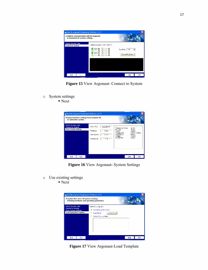
• Deployment If restarting an existing SonTek with no changes, the options are set.
o Direct system setup
Figure 14 View Argonaut- Session Type
Com1 baud rate: 9600 Connect to system Next
Figure 13 View Argonaut Recorder Screen- Format Files
17
Figure 15 View Argonaut- Connect to System
o System settings
Next
Figure 16 View Argonaut- System Settings
o Use existing settings
Next
Figure 17 View Argonaut-Load Template

18
o English units
Next
Figure 18 View Argonaut- Units
o Standard settings
Set system date/time
Figure 19 View Argonaut- Set Time
Match system to computer time Close next

19
Figure 20 View Argonaut- Match Computer Time
o Sampling interval
Set sampling interval to desired time length Next
Figure 21 View Argonaut- Data Interval
o Profiling settings
No profile Next
Figure 22 View Argonaut- Profile Settings

20
o Advanced settings
XYZ coordinate system next
Figure 23 View Argonaut- Coordinate System
o Burst mode
Disable burst mode
Figure 24 View Argonaut- Burst Mode
o Flow settings Double check channel dimensions Pick shape of pipe or canal Enter in dimensions Make sure to put the system elevation of the SonTek Next

21
Figure 25 View Argonaut- Channel Geometry
o Velocity calculations
Click on Theoretical flow calculation next
Figure 26 View Argonaut- Velocity Calculation
o Volume settings Select output units
i. Cfs and acre-ft Check total volume criteria
i. Add flow to total volume a. Enter value to when to add to total volume
Next

22
Figure 27 View Argonaut- Volume
o Output: current Enter flow parameters
i. Set channel flow and volume max Next
Figure 28 View Argonaut- Output Type
o Battery and Recorder Input battery options Next
Figure 29 View Argonaut- Battery

23
o Summary Save configuration file Next
Figure 30 View Argonaut- Summary
o Start deployment
Update system
Figure 31 View Argonaut- Update System
Start deployment
Figure 32 View Argonaut- Start Deployment

24
Figure 33 View Argonaut- Deployment Finished
o Exit
Unplug cable Click yes
Figure 34 View Argonaut- Exit
Statistical Method and Data Processing
The data comes in a file that can only be viewed in View Argonaut. The files first need to be converted into an Excel file before the data can be processed and be analyzed statistically. The steps to convert the files are outlined below. Processing Sontek Data
• Open View Argonaut
Figure 35 View Argonaut Icon

25
o Click on Processing
Figure 36 View Argonaut- Main Screen
Click on the open folder
Figure 37 View Argonaut- Processing Screen
Find the file
Figure 38 View Argonaut- Open File

26
Rename files (use start time) [location year month day time]
• Right click on file • Select rename
Open Ok
Figure 39 View Argonaut- Data Information
o Click on Processing after the file has opened
Figure 40 View Argonaut- Processing
Flow calc

27
Figure 41 View Argonaut- Flow Calculation
Double check info ok
Figure 42 View Argonaut- Channel Geometery
o File
Figure 43 View Argonaut- File

28
Export data
Figure 44 View Argonaut- Export Data
• Discharge data o Click on browse to select where the file will be
saved
Figure 45 View Argonaut- Discharge Data
• Export selected variable • Ok • Close

29
• Open Excel o Open- find folder (.dis)-discharge data o Open
Deliminated width o Copy (sample-flow)
Paste in master file Check volume summary
Once the data is in Excel, the flow values must be separated from the rest of the values. The master spreadsheet uses the flow rate to calculate the volume passing through the culvert. This value is then added up to get the total volume per day. The volume per day is then added up to have the total for each month. This value is used to compare the flows calculated by the SonTek, the DEID, and the FWUA which can be seen in the results section. The calibration points were used for the statistical analysis. The calibration points were obtained from a site visit. The flow rate was read from the external screens of the SonTek and venturi for 3 different periods of time. These flow rates were used to determine the standard deviation and uncertainty in Excel. The data sheet with these values can be seen in Appendix B.

30
RESULTS
The resulting data for multiple pairs of mean velocity and index velocity collected over a range of flows were analyzed using regression techniques, with and without multi-parameter ratings to account for the effect of stage. The resulting equation of the index velocity rating is necessary for using the internal flow computational feature on hydroacoustic flow meters or for post-processing data from temporary deployments. The goal was to check the accuracy of the volumetric readings from the SonTek flow meters by comparing them with the venturi meters that are currently being used for flow measurements. Table 1 shows the volumetric difference between the SonTek and the venturi meters at the different laterals, using TCCA-supplied data. Table 2 shows the volumetric difference between the SonTek and the venturi meters at the different laterals at DEID. Many irrigation districts and other water agencies are moving towards the SonTek Doppler flow meters for these types of sites in order to eliminate restrictive enclosed space access and the associated confined space entry requirements. However, the calibration of the units can take some time due to the number of data points required to adequately calibrate a field site.
Evaluation of TCCA Turnouts Table 1 Comparison of TCCA Turnouts after Dopplers Installed (SonTek-Venturi)
Site Sontek (acre-ft)
Venturi (acre-ft)
Difference (acre-ft)
% Difference from Venturi
OAWD 3* 8457 6906 1551 22.46% OAWD 4* 3784 3268 516 15.79% OAWD 5* 7469 6224 1245 20.00%
KWD 1 4835 4438 397 8.95% KWD 2 2650 2657 -7 -0.26% KWD 3 3105 3031 74 2.44% KWD 4 1757 1957 -200 -10.22% KWD 5 8257 7877 380 4.82% KWD 6 3888 3691 197 5.34% KWD 7 3127 3208 -81 -2.52% WWD 3 3831 4181 -350 -8.37% WWD 5 2090 1876 214 11.41% WWD 7 985 917 68 7.42% WWD 8 2575 2441 134 5.49%
WWD 9A 786 692 94 13.58% WWD 9B 1014 No BadgerCCWD 5 2749 2056 693 33.71% CCWD 7 5957 No BadgerDWD 3 2507 No BadgerDWD 4* 3899 2989 910 30.44%
*SonTek installed in beginning of 2009

31
Evaluation of DEID Laterals Table 2 Comparison of DEID Laterals after Dopplers Installed
(SonTek meter totals –Venturi meter totals)
Year Lat 40W (Acre-ft)
Lat 56W (Acre-ft)
Total Difference (Acre-ft)
Venturi meter total (Acre-ft) % Difference
2007 44 44 13780 0.32% 2008 -184 -184 16804 -1.09% 2009 -114 659 545 39238 1.39% 2010 482 627 1109 36001 3.21%
Figure 8 on the following page is a graphical representation of the data at DEID Lateral 56W in the years 2007, 2008, 2009 and part of 2010. Figure 9 on the page 19 is a graphical representation at DEID Lateral 40W for the year 2009 and part of 2010.

32
0
5000
10000
15000
20000
25000
30000
3/20 4/3 4/17 5/1 5/15 5/29 6/12 6/26 7/10 7/24 8/7 8/21 9/4 9/18 10/2 10/16 10/30 11/13
Volu
me
(acr
e-ft)
Date
Comparison of volume delivered to DEID lateral 56 West between two SonTek flow meters and FWUA's venturi and 2 propeller meters, 2007
SonTek Accumulated Volume FWUA Accumulated Volume DEID Accumulated Volume
April through October 2007% Dif f
SonTek = 13,780 acre-feet 0.32%FWUA = 13,736 acre-feet 0.0%DEID = 12,974 acre-feet -5.5%
% Dif f = Dif ference f rom FWUA/ FWUA total
0
5000
10000
15000
20000
25000
30000
5/24 6/7 6/21 7/5 7/19 8/2 8/16 8/30 9/13 9/27 10/11 10/25 11/8 11/22 12/6
Volu
me
(acr
e-ft)
Date
Comparison of volume delivered to DEID lateral 56 West between two SonTek flow meters and FWUA's venturi and 2 propeller meters, 2008
SonTek Accumulated Volume FWUA Accumulated Volume DEID Accumulated Volume
June through November 2008% Dif f
SonTek = 16,620 acre-feet -1.1%FWUA = 16,804 acre-feet 0.0%DEID = 16,407 acre-feet -2.4%
% Dif f = Dif ference f rom FWUA/ FWUA Total
No data for Jan‐Jun 2008
0
5000
10000
15000
20000
25000
30000
12/6 12/20 1/3 1/17 1/31 2/14 2/28 3/14 3/28 4/11 4/25 5/9 5/23 6/6 6/20 7/4 7/18 8/1 8/15 8/29 9/12 9/26 10/1010/24 11/7 11/21
Vol
ume
(acr
e-ft)
Date
Comparison of volume delivered to DEID lateral 56 West between two SonTek flow meters and FWUA's venturi and 2 propeller meters, 2009
SonTek Accumulated Volume FWUA Accumulated Volume DEID Accumulated Volume
January through October 2009% Dif f
SonTek = 24,375 acre-feet 2.8%FWUA = 23,716 acre-feet 0.0%DEID = 23,461 acre-feet -1.1%
% Dif f = Dif ference f rom FWUA/ FWUA Total
0
5000
10000
15000
20000
25000
30000
12/5 12/19 1/2 1/16 1/30 2/13 2/27 3/13 3/27 4/10 4/24 5/8 5/22 6/5 6/19 7/3 7/17 7/31 8/14 8/28 9/11 9/25 10/9 10/23 11/6 11/20
Vol
ume
(acr
e-ft)
Date
Comparison of volume delivered to DEID lateral 56 West between two SonTek flow meters and FWUA's venturi and 2 propeller meters, 2010
SonTek Accumulated Volume FWUA Accumulated Volume DEID Accumulated Volume
January through August 2010% Dif f
SonTek = 19,405 acre-feet 3.3%FWUA = 18,781 acre-feet 0.0%DEID = 18,506 acre-feet -1.5%
% Dif f= Difference f rom FWUA/ FWUA total
Figure 46 Volume graphs of Lateral 56W (2007-2010)

33
0
2000
4000
6000
8000
10000
12000
14000
16000
18000
2/14 2/28 3/14 3/28 4/11 4/25 5/9 5/23 6/6 6/20 7/4 7/18 8/1 8/15 8/29 9/12 9/26 10/10 10/24 11/7 11/2
Volu
me
(acr
e-ft)
Date
Comparison of volume delivered to DEID lateral 40 West between two SonTek flow meters and FWUA's venturi and 2 propeller meters, 2009
SonTek Accumulated Volume FWUA Accumulated Volume DEID Accumulated Volume
March through October 2009% Dif f
SonTek = 15,408 acre-feet -0.73%FWUA = 15,522 acre-feet 0.00%
DEID = 14,881 acre-feet -4.1%
% Dif ference= Dif ference f rom FWUA/ FWUA
Figure 47 Volume graphs of Lateral 40W (2009-2010)
0
2000
4000
6000
8000
10000
12000
14000
16000
18000
1/1 1/15 1/29 2/12 2/26 3/12 3/26 4/9 4/23 5/7 5/21 6/4 6/18 7/2 7/16 7/30 8/13 8/27 9/10 9/24 10/8 10/22 11/5 11/19
Volu
me
(acr
e-ft)
Date
Comparison of volume delivered to DEID lateral 40 West between two SonTek flow meters and FWUA's venturi and 2 propeller meters, 2010
SonTek Accumulated Volume FWUA Accumulated Volume DEID Accumulated Volume
Jan through October 2010% Dif
SonTek = 17,464 acre-feet 1.4%FWUA = 17,220 acre-feet 0.0%DEID = 16,613 acre-feet -3.5%
% Dif ference= Dif ference f rom FWUA/ FWUA

34
DISCUSSION
Data Comparison
The initial evaluation of the two DEID laterals from 2002 to 2005 (before installation of the Doppler meters) showed the following comparison between data measured by DEID and FWUA as seen in Table 3. DEID uses propeller meters for each water user and uses the total of all the meters to determine the total volume used per month. There is an issue with this because the meters are read at different times. The FWUA has a venturi meter at each lateral that is used for their monthly volume numbers.
Table 3 Comparison of DEID Turnouts to FWUA Laterals in acre-ft (DEID-FWUA)
Year 56W (acre-ft) 40W (acre-ft) Total Difference % Difference2002 Total -1452 -934 -2387 -4.9% 2003 Total -721 -818 -1539 -3.6% 2004 Total -1872 -1159 -3032 -6.2% 2005 Total -804 -558 -1362 -3.1% Grand Total (2002-2005) -4850 -3470 -8319 Average (2002-2005) -1212 -867 -2080 -4.5% The results of the current evaluation (shown in the Tables 4 and 5) reveal three items of significance:
1. The data from the venturi meters appears to be comparable to the data from the SonTeks at the two laterals where the equipment was installed. Comparing the data from 2002-2005 (Table 3) with the data from 2007-2010 (Table 4), the difference between the data measured by DEID and by FWUA has been reduced by more than 900 AF on average. One explanation for this reduction in the difference is that the venturi meters are being better maintained since this evaluation began.
2. The SonTek flow meters reported higher flow values than the FWUA venturi meters as seen in Table 5.
3. The average error was less than 1.0% when reporting the total volumes. Using the SonTek flow meters as the standard, the average loss calculated between the DEID propeller flow meters and the SonTek flow meters was 3.6%. This is a reasonable value considering conveyance losses and the potential for some under-reporting by propeller meters.

35
Evaluation of DEID Turnouts
Table 4 Comparison of DEID Turnouts after SonTeks Installed in acre-ft (DEID-FWUA)
56W 40W Total Difference % Difference 2007 Total -762 -822 -1584 -6.4% 2008 Total -397 -587 -984 -3.3% 2009 Total -255 -641 -896 -2.3% 2010 Total* -275 -411 -686 -2.1% Totals -1689 -2461 -4150 Average -422 -615 -1038 -3.5%
Table 5 Comparison of DEID Turnouts after SonTeks Installed in acre-ft (SonTek-FWUA)
Year 40W 56W Total Difference % Difference 2007 44 44 0.32% 2008 -184 -184 -1.09% 2009 -114 659 545 1.39% 2010 482 627 1109 3.21% Total 368 1146 1514 3.82% Average 184 286.5 378.5 0.96%
%
100% *2010 data is from Jan-August 2010
Statistical Calibration Discussion
In past studies, ITRC has used the R-Squared statistic to set the minimum number of data points. After reviewing the literature it was found that USGS uses 1 standard deviation to describe measurement sites and a simple rating to rate the site. Table 6 shows the impact of using the USGS statistical calculations to evaluate the minimum number of points required.
Table 6 Statistical evaluation of the DEID laterals
USGS – 1 Standard Deviation ITRC- Uncertainty “Excellent” means ≤ 2% “Excellent” means ≤ 4%
“Good” means ≤ 5% “Good” means ≤ 10% “Fair” means ≤ 8% “Fair” means ≤ 16% “Poor” means ≥ 8% “Poor” means ≥ 16%
Tables 7 and 8 shows the results from Laterals 56W and 40W and Tables 9 and 10 shows the results from the TCCA laterals. Note that although R-Squared is considered high

36
(>0.99) for many of the examples, the relative uncertainty is very poor until at least 8 data points are obtained in these examples. More data points are generally encouraged to improve the reporting of the volumetric accuracy and to regularly verify the meters are all working properly. The recommended “relative uncertainty” value of 8% is considered “good.” Both DEID and TCCA laterals meet these calibration criteria when at least 8 data points are used. The more data points collected, the smaller the uncertainty is. The uncertainty can be reduced by using additional data points but it takes time and money to get calibration points for each of the laterals. The field calibration is expensive so it is beneficial to use a model. The model needs to have similar hydraulic conditions as the field installation. This makes it so the calibration can still be done but at a smaller scale making it less expensive. Table 8 shows the results from the TCCA laterals. The recommended one standard deviation value of 5% is considered “good.” The TCCA tries to calibrate the venturi every month to ensure good measurements. The relative uncertainty was first used after the r-squared statistic to rate an installation; however, it was hard for people to understand. There are many statistical formulas that can be used to calculate uncertainty and there is no one standard equation accepted for determining uncertainty. The uncertainty values found in Tables 8 and 10 were found using the Linest function in Excel. These values can be found on the calibration sheets in Appendix B. The standard deviation was also used to rate each site (using the USGS ratings system) since it is a more commonly used equation and more people are familiar with the term. Tables 7-10 include a column titled “Slope.” The ideal slope would be 1.0 which would mean the SonTek and the venturi have the same flow rate. 7 out of the 10 laterals had a smaller slope than 1 which means the venturi had a larger flow rate than the SonTek. The other 3 laterals had a larger slope so the SonTek had a larger flow rate than the venturi. In most cases the more data points collected the closer the slope got to one, so the flow rate of the two devices were getting closer to the same number.
Table 7 Summary of the results from Lat 56 and Lat 40
Site Std Dev R-Squared Slope DEID 56W-4 points 2.8% 0.989 0.8599 DEID 56W-8 points 2.1% 0.995 0.8680 DEID 56W-12 points 2.2% 0.996 0.8782 DEID 56W-14 points 2.8% 0.996 0.8701 DEID 40W-4 points 1.9% 0.988 0.6964 DEID 40W-8 points 4.2% 0.994 0.8842 DEID 40W-10 points 3.57% 0.997 0.8762
37
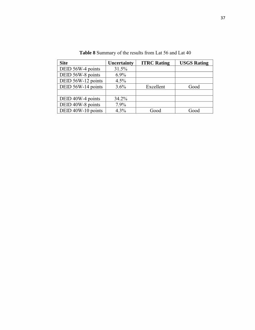
Table 8 Summary of the results from Lat 56 and Lat 40
Site Uncertainty ITRC Rating USGS Rating DEID 56W-4 points 31.5% DEID 56W-8 points 6.9% DEID 56W-12 points 4.5% DEID 56W-14 points 3.6% Excellent Good DEID 40W-4 points 34.2% DEID 40W-8 points 7.9% DEID 40W-10 points 4.3% Good Good

38
Table 9 Summary of the results from TCCA laterals
Site Std Dev
R-Squared Slope
CCWD 5- 4 points 1.40% 0.9986 0.8326 CCWD 5- 10 points 3.45% 0.9957 0.8579 CCWD 5 -20 points 8.52% 0.9887 0.8601 CCWD 5- 28 points 7.84% 0.9900 0.8435 CCWD 7A- 4 points 2.48% 0.9995 0.9394 CCWD 7A- 10 points 4.78% 0.9944 0.9893 CCWD 7A- 11 points 4.57% 0.9962 0.9855 DWD 3- 4 points 5.15% 0.9686 1.0766 DWD 3- 10 points 10.28% 0.9818 0.7868 DWD 3- 14 points 8.78% 0.9864 0.7964 DWD 4- 4 points 32.42% 0.7880 0.7881 DWD 4- 8 points 21.70% 0.8120 0.8122 DWD 4- 9 points 21.30% 0.8790 0.8789 WWD 5- 4 points 1.90% 0.9992 0.8906 WWD 5- 10 points 6.68% 0.9976 0.9211 WWD 5- 11 points 6.51% 0.9961 0.9171 WWD 7- 4 points 10.58% 0.9748 0.8388 WWD 7- 10 points 8.45% 0.9817 0.8667 WWD 7- 18 points 6.43% 0.9830 0.8789 WWD 8- 4 points 2.73% 0.9954 1.1186 WWD 8- 10 points 7.05% 0.9900 1.0844 WWD 8- 14 points 7.87% 0.9875 1.0988 WWD 9B- 4 points 15.10% 0.9260 1.0381 WWD 9B- 10 points 11.25% 0.9769 0.9869 WWD 9B- 12 points 10.46% 0.9703 0.9559

39
Table 10 Summary of the results of TCCA laterals
Site UncertaintyITRC Rating
USGS Rating
CCWD 5- 4 points 11.32% CCWD 5- 10 points 5.34% CCWD 5 -20 points 5.30% CCWD 5- 28 points 4.55% Good Fair CCWD 7A- 4 points 6.92% CCWD 7A- 10 points 6.12% CCWD 7A- 11 points 4.65% Good Good DWD 3- 4 points 54.80% DWD 3- 10 points 11.09% DWD 3- 14 points 7.38% Good Poor DWD 4- 4 points 98.02% DWD 4- 8 points 26.32% DWD 4- 9 points 13.59% Fair Poor WWD 5- 4 points 8.52% WWD 5- 10 points 4.00% WWD 5- 11 points 4.74% Good Fair WWD 7- 4 points 48.87% WWD 7- 10 points 11.12% WWD 7- 18 points 6.97% Good Fair WWD 8- 4 points 20.77% WWD 8- 10 points 8.20% WWD 8- 14 points 7.08% Good Fair WWD 9B- 4 points 85.98% WWD 9B- 10 points 12.54% WWD 9B- 12 points 12.33% Fair Poor

40
RECOMMENDATIONS
The SonTek SW flow meter will provide a more reliable volumetric reading over the water season and will be a good replacement for the older technology when it has been fully calibrated. The venturi meter is still an accurate instantaneous device and can be used to check the calibration of the SonTek SW flow meter. Time is needed after installing the SonTek before switching over to insure a good calibration procedure. Collecting calibration points takes a lot of time and 10 or more data points should be used to calibrate a site. The DEID laterals have a consistent slope value for rectangular pipes of 0.85. The TCCA laterals have a consistent slope value for round pipes of 0.92. To ensure good calibration the venturi needs to be properly maintained and calibrated often. The calibration procedure for TCCA can be seen in Appendix D. The FWUA calibrates the venturi 4 times a year when they have time. It would be recommended that the venturi be calibrated more often to ensure accurate readings.

41
REFERENCES
Clemmens, A.J. and Brian Wahlin. 2006. Accuracy of Annual Volume from Current-Meter-Based Stage Discharges. ASCE, Journal of Hydrologic Engineering 11(5): 489-501.
Howes D., Burt C.M., and Sanders B.F. 2010. Subcritical Contraction for Improved Open-Channel Flow Measurement Accuracy with an Upward-Looking ADVM. J. Irrig. Drain. Eng., 136(9), 617-626.
Huhta, C., and Ward, C. 2003. Flow measurements using an upwardlooking Argonaut-SW Doppler current meter. Proc., IEEE/OES 7th Working Conf. on Current Measurement Technology, San Diego, 35– 39.
Irrigation Training and Research Center (ITRC). 2005. Hydroacoustic meters. Irrigation Training and Research Center, California Polytechnic State Univ., San Luis Obispo, Calif.
Rehmel, Michael. 2007. Application of Acoustic Doppler Velocimeters for Streamflow Measurements. ASCE, Journal of Hydrologic Engineering 133(12): 1433-1438.
SonTek YSI Incorporated. 2009. SonTek YSI Incorporated Home Page. <http://www.sontek.com/>, October 22, 2010.
Styles, S. W., Busch, B., Howes, D., and Cardenas, M. 2006. Nonstandard structure flow measurement evaluation using the flow rate indexing procedure-QIP. R 06-003, Irrigation Training and Research Center, California Polytechnic State Univ., San Luis Obispo, Calif. http://www.itrc.org/reports/qip/r06003.pdf.
Trout, Thomas and Bruce Mackey. 1988. Furrow Flow Measurement Accuracy. ASCE, Journal of Irrigation and Drainage Engineering 114(2):244-255.
U. S. Department of the Interior Bureau of Reclamation. 2001. Water Measurement Manual. Washington, D.C.
Vermeyen, T. B. 2000. A laboratory evaluation of Unidata’s Starflow Doppler flowmeter and MGD technologies’ acoustic Doppler flowmeter. Proc., Joint Conf. on Water Resource Engineering and Water Resources Planning and Management, Minneapolis, ASCE, 318.
Ward, C.J., Kibby K., Nauman, R. 2007. Upgrading the Flow Measurement System at the Tehama Colusa Canal Authority. http://www.hydroscientificwest.com/pdfs/ TCCA.pdf

42
APPENDIX A
How Project Meets Requirements for the BRAE Major

43
California Polytechnic State University 10‐June‐11 BioResource and Agricultural Engineering Department Groundwater, Lynn BRAE Senior Project Contract ID #00338686 BRAEProject Title Evaluate the accuracy of the Sontek Doppler Flow Meters in large diameter pipes in water districts.
Background Information Sontek doppler flow meters are used to measure the flow going through a pipeline or canal. Water districts need to measure the flow in order to bill their customers for the correct amount of water. Water districts currently use various flow measurement devices such as a venturi meter, magnetic meter, or a Sontek flow meter. Water districts are switching over to Sontek meters because it eliminates confined space entry requirements and is easier to maintain.
Statement of Work The first phase of this senior project will be to evaluate points (volumetric readings at a point in time) for the currently used venturi meters and the sontek flow meters. The two cooperating districts are the Delano Earlimart Irrigation District and the Tehama Colusa Canal Authority. The second phase will be to run a statistical analysis on the data and determine the uncertainty. Uncertainty is how one determines how accurate a meter is. The third phase will be to compile the results to evaluate the accuracy of the Sontek flow meters versus the venturi meters.
How Project Meets Requirements for the BRAE Major Major Design Experience - The project must incorporate a major design experience. Design is the process of devising a system, component, or process to meet specific needs. The design process typically includes the following fundamental elements. Explain how this project will address these issues. (Insert N/A for any item not applicable to this project.)
Establishment of objectives and criteria
Project objectives and criteria are established to meet the needs of the water district and USBR standards for flow measurement.
Synthesis and analysis
The project will incorporate QC through ITRC and statistical analysis of the sites using FlowPack
Construction, testing and evaluation N/A
Incorporation of applicable engineering standards The project will utilize USBR standards for flow measurement.

44
Capstone Design Experience ‐ The engineering design project must be based on the knowledge and skills acquired in earlier coursework (Major, Support and/or GE courses).
Incorporates knowledge/ skills from these key courses
129 Lab Skills/Safety, 216 Principles of Irrigation, 312 Fluid Hydraulics, 331 Irrigation Theory, 414 Irrigation Design, CSC 232 Computer Programming , 216 Fundamentals of Electricity, 328 Measurements and Computer Interfacing, Technical Writing
Design Parameters and Constraints - The project should address a significant number of the categories of constraints listed below. (Insert N/A for any area not applicable to this project.)
Physical
The flow meters have already been installed based on the physical constraints of the existing pipe and/or channels. Accurate measurement of the pipes and channels is necessary to ensure the accuracy of the flow meters.
Economic Installation, operation and maintenance costs will be an important
factor in the water districts' decision making process.
Environmental
The flow meters must be able to operate under the full range of environmental conditions that they will encounter in the field (i.e., temperature extremes, humidity, rain, wind, dust, etc.)
Sustainability
The flow metering equipment must be capable of operating continuously for long periods of time and last a number of years before requiring major maintenance or replacement.
Manufacturability N/A
Health and Safety Health and safety considerations for the operation and maintenance
of the flow meters must be identified. Ethical N/A Social N/A
Political Implementation of the project 's recommendation will be subject to
approval of the governing board of each water district. Aesthetic N/A the flow meters have already been installed.
Other ‐ Productivity The man‐hours required to operate and maintain the flow meters
must be factored into the economic analysis. Other

45
List of Tasks and Time Estimate
TASK Hours Research in library on flow measurement 10 Data Evaluation 50 Statistical Analysis 75 FlowPack Analysis 25
Preparation of written report 40
TOTAL 200
Financial Responsibility
Preliminary estimate of project costs: $100
Finances approved by (signature of Project Sponsor):
Final Report Due: June 10, 2011 Number of Copies: 3
Approval Signatures Date Student:
Project
Supervisor:
Department
Head:

46
APPENDIX B
Calibration Sheets

DEID 40 calibration data- 10 pointsCalibration following procedure by Flow Measurement Manual, USBR Chapter 3
DateSonTek
Discharge (cfs)Venturi
Discharge (cfs)
Adjusted Discharge
(cfs) Error
Percent Deviation of Discharge Bin Frequency
Qact Qcs Qeq deltaQ% -4.00% -0.04 14/22/2009 25.1 28.2 26.2 -2.05 -7.26% -2.00% -0.02 15/13/2009 43.0 39.9 41.9 2.01 5.05% 0.00% 0 35/28/2009 47.6 43.7 45.9 2.24 5.13% 2.00% 0.02 36/16/2009 44.0 42.5 42.8 0.30 0.70% 4.00% 0.04 09/10/2009 43.5 42.8 42.3 -0.52 -1.22% 6.00% 0.06 29/10/2009 92.6 85.5 85.4 -0.12 -0.14% More 09/15/2009 37.7 37.6 37.2 -0.39 -1.03%9/15/2009 81.0 77.2 75.1 -2.03 -2.63%6/17/2010 60.0 56.6 56.8 0.17 0.30%6/17/2010 123.6 112.1 112.5 0.39 0.34%
calibration equation is y = 0.8762x + 4.195 from chart
standard deviation 3.57%
Qventuri = m(QSonTek) + b
m b0.876 4.19501
Standard errors of m and b 0.0166 1.0989
r2 Std. Erry estimate 0.9971 1.5032
Fdegrees of
freedom 2796.8112 8Regression sum of squares
Residual sum of squares 6319.6572 18.0768
Confidence Level = 68%α = 32%Tα,ν = 1.060Confidence Interval on m 0.8586Uncertainty on m ± 0.018Relative uncertainty on m, % ± 2.00 %Confidence Interval on b 3.0299Uncertainty on b ± 1.165Relative uncertainty on b, % 27.77%
REGRESSION TO PREDICT VENTURI OUTPUT FROM SONTEK INDEX FLOW MEASUREMENT - Tony Wahl (USBR)
0
1
2
3
4
-4.0% -2.0% 0.0% 2.0% 4.0% 6.0%
Occ
urre
nces
Percent Deviation of Discharge
Histogram of Percent Deviation of Discharge
y = 0.8762x + 4.1950R² = 0.9971
0.0
20.0
40.0
60.0
80.0
100.0
120.0
0.0 20.0 40.0 60.0 80.0 100.0 120.0 140.0
47
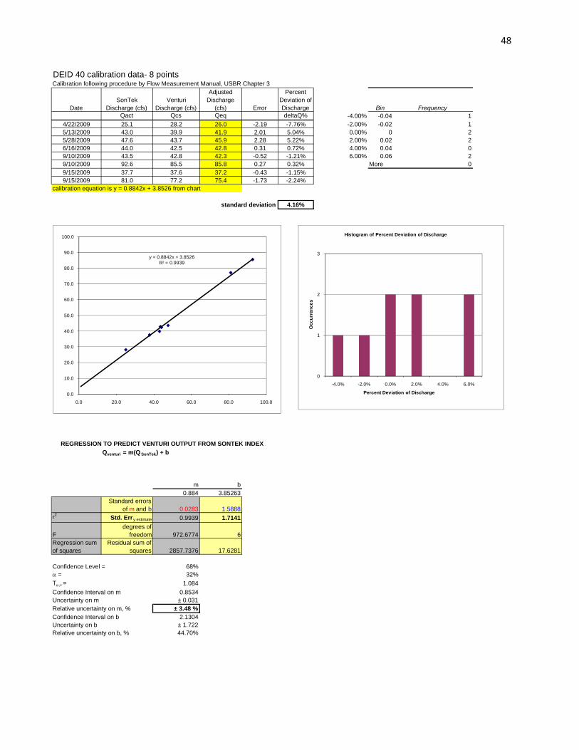
DEID 40 calibration data- 8 pointsCalibration following procedure by Flow Measurement Manual, USBR Chapter 3
DateSonTek
Discharge (cfs)Venturi
Discharge (cfs)
Adjusted Discharge
(cfs) Error
Percent Deviation of Discharge Bin Frequency
Qact Qcs Qeq deltaQ% -4.00% -0.04 14/22/2009 25.1 28.2 26.0 -2.19 -7.76% -2.00% -0.02 15/13/2009 43.0 39.9 41.9 2.01 5.04% 0.00% 0 25/28/2009 47.6 43.7 45.9 2.28 5.22% 2.00% 0.02 26/16/2009 44.0 42.5 42.8 0.31 0.72% 4.00% 0.04 09/10/2009 43.5 42.8 42.3 -0.52 -1.21% 6.00% 0.06 29/10/2009 92.6 85.5 85.8 0.27 0.32% More 09/15/2009 37.7 37.6 37.2 -0.43 -1.15%9/15/2009 81.0 77.2 75.4 -1.73 -2.24%
calibration equation is y = 0.8842x + 3.8526 from chart
standard deviation 4.16%
Qventuri = m(Q SonTek) + b
m b0.884 3.85263
Standard errors of m and b 0.0283 1.5888
r2 Std. Erry estimate 0.9939 1.7141
Fdegrees of
freedom 972.6774 6Regression sum of squares
Residual sum of squares 2857.7376 17.6281
Confidence Level = 68%α = 32%Tα,ν = 1.084Confidence Interval on m 0.8534Uncertainty on m ± 0.031Relative uncertainty on m, % ± 3.48 %Confidence Interval on b 2.1304Uncertainty on b ± 1.722Relative uncertainty on b, % 44.70%
REGRESSION TO PREDICT VENTURI OUTPUT FROM SONTEK INDEX
0
1
2
3
-4.0% -2.0% 0.0% 2.0% 4.0% 6.0%
Occ
urre
nces
Percent Deviation of Discharge
Histogram of Percent Deviation of Discharge
y = 0.8842x + 3.8526R² = 0.9939
0.0
10.0
20.0
30.0
40.0
50.0
60.0
70.0
80.0
90.0
100.0
0.0 20.0 40.0 60.0 80.0 100.0
48

DEID 40 calibration data- 4 pointsCalibration following procedure by Flow Measurement Manual, USBR Chapter 3
DateSonTek
Discharge (cfs)Venturi
Discharge (cfs)
Adjusted Discharge
(cfs) Error
Percent Deviation of Discharge Bin Frequency
Qact Qcs Qeq deltaQ% -4.00% -0.04 04/22/2009 25.1 28.2 28.2 0.00 0.00% -2.00% -0.02 15/13/2009 43.0 39.9 40.7 0.83 2.08% 0.00% 0 05/28/2009 47.6 43.7 43.9 0.24 0.54% 2.00% 0.02 26/16/2009 44.0 42.5 41.4 -1.07 -2.51% 4.00% 0.04 1
calibration equation is y = 0.6964x + 10.7485 from chart 6.00% 0.06 0More 0
standard deviation 1.91%
Qventuri = m(Q SonTek) + b
m b0.696 10.74848
Standard errors of m and b 0.0554 2.2649
r2 Std. Erry estimate 0.9875 0.9694
Fdegrees of
freedom 157.8816 2Regression sum of squares
Residual sum of squares 148.3619 1.8794
Confidence Level = 68%α = 32%Tα,ν = 1.312Confidence Interval on m 0.6237Uncertainty on m ± 0.073Relative uncertainty on m, % ± 10.44 %Confidence Interval on b 7.7779Uncertainty on b ± 2.971Relative uncertainty on b, % 27.64%
REGRESSION TO PREDICT VENTURI OUTPUT FROM SONTEK INDEX
0
1
2
3
-4.0% -2.0% 0.0% 2.0% 4.0% 6.0%
Occ
urre
nces
Percent Deviation of Discharge
Histogram of Percent Deviation of Discharge
y = 0.6964x + 10.7485R² = 0.9875
0.0
5.0
10.0
15.0
20.0
25.0
30.0
35.0
40.0
45.0
50.0
0.0 10.0 20.0 30.0 40.0 50.0
49

DEID 56 calibration data- 14 pointsCalibration following procedure by Flow Measurement Manual, USBR Chapter 3
DateSonTek
Discharge (cfs)Venturi
Discharge (cfs)
Adjusted Discharge
(cfs) Error
Percent Deviation of Discharge Bin Frequency
Qact Qcs Qeq deltaQ% -4.00% -0.04 06/7/2007 81.9 74.2 76.6 2.37 3.19% -2.00% -0.02 37/12/2007 106.8 99.4 98.3 -1.16 -1.16% 0.00% 0 69/16/2008 50.4 50.1 49.1 -0.99 -1.97% 2.00% 0.02 210/16/2008 72.7 71.1 68.5 -2.57 -3.62% 4.00% 0.04 24/22/2009 23.4 26.3 25.7 -0.65 -2.47% 6.00% 0.06 05/13/2009 66.2 62.9 62.9 -0.01 -0.01% More 15/28/2009 68.4 64.7 64.8 0.06 0.10%6/16/2009 55.8 53.1 53.8 0.70 1.31%9/10/2009 49.2 46.7 48.2 1.44 3.08%9/10/2009 100.6 94.3 92.8 -1.43 -1.52%9/15/2009 31.2 33.0 32.5 -0.54 -1.62%9/15/2009 67.0 65.5 63.7 -1.80 -2.75%6/17/2010 103.2 89.2 95.1 5.89 6.60%6/17/2010 196.3 177.5 176.2 -1.32 -0.74%
calibration equation is y = 0.87x + 5.308 from chart
standard deviation 2.80%
Qventuri = m(QSonTek) + b
m b0.870 5.308
Standard errors of m and b 0.0145 1.2601
r2 Std. Erry estimate 0.9967 2.2266
Fdegrees of
freedom 3605.4290 12Regression sum of squares
Residual sum of squares 17874.5920 59.4923
Confidence Level = 68%α = 32%Tα,ν = 1.037Confidence Interval on m 0.8551Uncertainty on m ± 0.015Relative uncertainty on m, % ± 1.73 %Confidence Interval on b 4.0007Uncertainty on b ± 1.307Relative uncertainty on b, % 24.63%
REGRESSION TO PREDICT VENTURI OUTPUT FROM SONTEK INDEX FLOW MEASUREMENT - Tony Wahl (USBR)
0
1
2
3
4
5
6
7
-4.0% -2.0% 0.0% 2.0% 4.0% 6.0%
Occ
urre
nces
Percent Deviation of Discharge
Histogram of Percent Deviation of Discharge
y = 0.8701x + 5.3079R² = 0.9967
0.0
20.0
40.0
60.0
80.0
100.0
120.0
140.0
160.0
180.0
200.0
0.0 50.0 100.0 150.0 200.0 250.0
50

DEID 56 calibration data- 12 pointsCalibration following procedure by Flow Measurement Manual, USBR Chapter 3
DateSonTek
Discharge (cfs)Venturi
Discharge (cfs)
Adjusted Discharge
(cfs) Error
Percent Deviation of Discharge Bin Frequency
Qact Qcs Qeq deltaQ% -4.00% -0.04 06/7/2007 81.9 74.2 77.1 2.89 3.90% -2.00% -0.02 37/12/2007 106.8 99.4 99.0 -0.43 -0.44% 0.00% 0 49/16/2008 50.4 50.1 49.4 -0.72 -1.43% 2.00% 0.02 310/16/2008 72.7 71.1 69.0 -2.13 -2.99% 4.00% 0.04 24/22/2009 23.4 26.3 25.7 -0.60 -2.28% 6.00% 0.06 05/13/2009 66.2 62.9 63.3 0.39 0.62% More 05/28/2009 68.4 64.7 65.2 0.47 0.73%6/16/2009 55.8 53.1 54.1 1.01 1.90%9/10/2009 49.2 46.7 48.4 1.70 3.64%9/10/2009 100.6 94.3 93.5 -0.76 -0.81%9/15/2009 31.2 33.0 32.6 -0.42 -1.28%9/15/2009 67.0 65.5 64.1 -1.40 -2.13%
calibration equation is y = 0.8782x + 5.1712 from chart
standard deviation 2.26%
Qventuri = m(QSonTek) + b
m b0.878 5.171
Standard errors of m and b 0.0176 1.2061
r2 Std. Erry estimate 0.9960 1.4468
Fdegrees of
freedom 2502.7456 10Regression sum of squares
Residual sum of squares 5238.5054 20.9310
Confidence Level = 68%α = 32%Tα,ν = 1.046Confidence Interval on m 0.8598Uncertainty on m ± 0.018Relative uncertainty on m, % ± 2.09 %Confidence Interval on b 3.9092Uncertainty on b ± 1.262Relative uncertainty on b, % 24.41%
REGRESSION TO PREDICT VENTURI OUTPUT FROM SONTEK INDEX
0
1
2
3
4
5
-4.0% -2.0% 0.0% 2.0% 4.0% 6.0%
Occ
urre
nces
Percent Deviation of Discharge
Histogram of Percent Deviation of Discharge
y = 0.8782x + 5.1712R² = 0.9960
0.0
20.0
40.0
60.0
80.0
100.0
120.0
0.0 20.0 40.0 60.0 80.0 100.0 120.0
51

DEID 56 calibration data- 8 pointsCalibration following procedure by Flow Measurement Manual, USBR Chapter 3
DateSonTek
Discharge (cfs)Venturi
Discharge (cfs)
Adjusted Discharge
(cfs) Error
Percent Deviation of Discharge Bin Frequency
Qact Qcs Qeq deltaQ% -4.00% -0.04 06/7/2007 81.9 74.2 76.8 2.62 3.53% -2.00% -0.02 17/12/2007 106.8 99.4 98.5 -0.96 -0.97% 0.00% 0 39/16/2008 50.4 50.1 49.4 -0.67 -1.34% 2.00% 0.02 310/16/2008 72.7 71.1 68.8 -2.31 -3.25% 4.00% 0.04 14/22/2009 23.4 26.3 26.0 -0.28 -1.07% 6.00% 0.06 05/13/2009 66.2 62.9 63.2 0.27 0.43% More 05/28/2009 68.4 64.7 65.1 0.34 0.52%6/16/2009 55.8 53.1 54.1 1.00 1.88%
calibration equation is y = 0.868x + 5.7276 from chart
standard deviation 2.10%
Qventuri = m(QSonTek) + b
m b0.868 5.728
Standard errors of m and b 0.0244 1.6986
r2 Std. Erry estimate 0.9953 1.5710
Fdegrees of
freedom 1261.2877 6Regression sum of squares
Residual sum of squares 3112.8510 14.8080
Confidence Level = 68%α = 32%Tα,ν = 1.084Confidence Interval on m 0.8415Uncertainty on m ± 0.026Relative uncertainty on m, % ± 3.05 %Confidence Interval on b 3.8864Uncertainty on b ± 1.841Relative uncertainty on b, % 32.15%
REGRESSION TO PREDICT VENTURI OUTPUT FROM SONTEK INDEX
0
1
2
3
4
-4.0% -2.0% 0.0% 2.0% 4.0% 6.0%
Occ
urre
nces
Percent Deviation of Discharge
Histogram of Percent Deviation of Discharge
y = 0.8680x + 5.7276R² = 0.9953
0.0
20.0
40.0
60.0
80.0
100.0
120.0
0.0 20.0 40.0 60.0 80.0 100.0 120.0
52

DEID 56 calibration data- 4 pointsCalibration following procedure by Flow Measurement Manual, USBR Chapter 3
DateSonTek
Discharge (cfs)Venturi
Discharge (cfs)
Adjusted Discharge
(cfs) Error
Percent Deviation of Discharge Bin Frequency
Qact Qcs Qeq deltaQ% -4.00% -0.04 06/7/2007 81.9 74.2 77.1 2.92 3.93% -2.00% -0.02 17/12/2007 106.8 99.4 98.6 -0.86 -0.87% 0.00% 0 29/16/2008 50.4 50.1 50.0 -0.12 -0.24% 2.00% 0.02 010/16/2008 72.7 71.1 69.2 -1.93 -2.72% 4.00% 0.04 1
calibration equation is y = 0.8599x + 6.6892 from chart 6.00% 0.06 0More 0
standard deviation 2.81%
Qventuri = m(QSonTek) + b
m b0.860 6.689
Standard errors of m and b 0.0630 5.0715
r2 Std. Erry estimate 0.9894 2.5494
Fdegrees of
freedom 186.4080 2Regression sum of squares
Residual sum of squares 1211.5359 12.9988
Confidence Level = 68%α = 32%Tα,ν = 1.312Confidence Interval on m 0.7773Uncertainty on m ± 0.083Relative uncertainty on m, % ± 9.61 %Confidence Interval on b 0.0375Uncertainty on b ± 6.652Relative uncertainty on b, % 99.44%
REGRESSION TO PREDICT VENTURI OUTPUT FROM SONTEK INDEX
0
1
2
3
-4.0% -2.0% 0.0% 2.0% 4.0% 6.0%
Occ
urre
nces
Percent Deviation of Discharge
Histogram of Percent Deviation of Discharge
y = 0.8599x + 6.6892R² = 0.9894
0.0
20.0
40.0
60.0
80.0
100.0
120.0
0.0 20.0 40.0 60.0 80.0 100.0 120.0
53

CCWD 5 calibration data- 28 pointsCalibration following procedure by Flow Measurement Manual, USBR Chapter 3
DateSonTek
Discharge (cfs)Venturi
Discharge (cfs)
Adjusted Discharge
(cfs) Error
Percent Deviation of Discharge Bin Frequency
Qact Qcs Qeq deltaQ% -4.00% -0.04 54/6/2009 10.81 8.8 8.8 -0.04 -0.43% -2.00% -0.02 64/10/2009 7.87 6.3 6.3 0.03 0.46% 0.00% 0 24/24/2009 3.92 3.1 3.0 -0.11 -3.45% 2.00% 0.02 34/27/2009 7.61 6.3 6.1 -0.19 -2.98% 4.00% 0.04 25/4/2009 4.10 3.0 3.1 0.17 5.58% 6.00% 0.06 25/15/2009 7.10 5.9 5.7 -0.20 -3.41% More 35/17/2009 3.71 3.0 2.8 -0.17 -5.59%5/18/2009 4.11 3.1 3.1 0.05 1.52%5/22/2009 3.83 3.0 2.9 -0.06 -2.18%5/23/2009 7.65 6.4 6.1 -0.32 -5.03%5/29/2009 7.87 5.6 6.3 0.71 12.68%5/30/2009 11.81 9.0 9.6 0.68 7.55%7/18/2009 18.97 15.3 15.7 0.36 2.33%7/23/2009 20.15 17.9 16.7 -1.19 -6.68%8/8/2009 3.53 3.2 2.6 -0.55 -17.23%8/10/2009 8.12 6.7 6.5 -0.21 -3.13%8/14/2009 7.68 6.5 6.1 -0.36 -5.46%8/22/2009 11.41 9.4 9.3 -0.13 -1.38%9/25/2009 4.94 3.1 3.8 0.75 24.29%10/1/2009 3.96 3.1 3.0 -0.07 -2.38%3/5/2010 4.08 3.1 3.1 0.03 0.89%3/19/2010 16.26 13.1 13.4 0.30 2.29%3/26/2010 16.87 13.4 13.9 0.54 4.04%4/16/2010 12.40 10.3 10.1 -0.15 -1.45%4/24/2010 8.88 6.9 7.2 0.27 3.97%4/24/2010 12.96 10.0 10.6 0.58 5.77%5/8/2010 19.41 15.5 16.0 0.53 3.45%5/17/2010 22.81 18.8 18.9 0.16 0.83%
standard deviation 7.84%
Qventuri = m(QSonTek) + b
m b0.843 -0.336
Standard errors of m and b 0.0185 0.1831
r2 Std. Erry estimate 0.9900 0.4472
Fdegrees of
freedom 2089.1489 21Regression sum of squares
Residual sum of squares 417.7504 4.1992
Confidence Level = 68%α = 32%Tα,ν = 1.019Confidence Interval on m 0.8247Uncertainty on m ± 0.019Relative uncertainty on m, % ± 2.23 %Confidence Interval on b -0.5228Uncertainty on b ± 0.186Relative uncertainty on b, % -55.45%
REGRESSION TO PREDICT VENTURI OUTPUT FROM SONTEK INDEX FLOW MEASUREMENT - Tony Wahl (USBR)
0
1
2
3
4
5
6
7
-4.0% -2.0% 0.0% 2.0% 4.0% 6.0%
Occ
urre
nces
Percent Deviation of Discharge
Histogram of Percent Deviation of Discharge
y = 0.8435x - 0.3363R² = 0.9900
-20.0
-15.0
-10.0
-5.0
0.0
5.0
10.0
15.0
20.0
0.00 5.00 10.00 15.00 20.00 25.00
54

CCWD 5 calibration data- 20 pointsCalibration following procedure by Flow Measurement Manual, USBR Chapter 3
DateSonTek
Discharge (cfs)Venturi
Discharge (cfs)
Adjusted Discharge
(cfs) Error
Percent Deviation of Discharge Bin Frequency
Qact Qcs Qeq deltaQ% -4.00% -0.04 64/6/2009 10.81 8.8 8.9 0.05 0.60% -2.00% -0.02 5
4/10/2009 7.87 6.3 6.3 0.07 1.13% 0.00% 0 14/24/2009 3.92 3.1 3.0 -0.13 -4.22% 2.00% 0.02 34/27/2009 7.61 6.3 6.1 -0.15 -2.38% 4.00% 0.04 15/4/2009 4.10 3.0 3.1 0.14 4.88% 6.00% 0.06 1
5/15/2009 7.10 5.9 5.7 -0.17 -2.92% More 35/17/2009 3.71 3.0 2.8 -0.19 -6.51%5/18/2009 4.11 3.1 3.1 0.03 0.84%5/22/2009 3.83 3.0 2.9 -0.09 -3.04%5/23/2009 7.65 6.4 6.2 -0.29 -4.44%5/29/2009 7.87 5.6 6.3 0.75 13.43%5/30/2009 11.81 9.0 9.7 0.78 8.75%7/18/2009 18.97 15.3 15.9 0.58 3.81%7/23/2009 20.15 17.9 16.9 -0.95 -5.30%8/8/2009 3.53 3.2 2.6 -0.58 -18.18%
8/10/2009 8.12 6.7 6.6 -0.16 -2.45%8/14/2009 7.68 6.5 6.2 -0.32 -4.87%8/22/2009 11.41 9.4 9.4 -0.03 -0.31%9/25/2009 4.94 3.1 3.8 0.74 24.06%10/1/2009 3.96 3.1 3.0 -0.10 -3.13%
standard deviation 8.52%
Qventuri = m(QSonTek) + b
m b0.860 -0.425
Standard errors of m and b 0.0217 0.2000
r2 Std. Erry estimate 0.9887 0.4510
Fdegrees of
freedom 1569.5825 18Regression sum of squares
Residual sum of squares 319.3018 3.6618
Confidence Level = 68%α = 32%Tα,ν = 1.023Confidence Interval on m 0.8379Uncertainty on m ± 0.022Relative uncertainty on m, % ± 2.58 %Confidence Interval on b -0.6299Uncertainty on b ± 0.205Relative uncertainty on b, % -48.10%
REGRESSION TO PREDICT VENTURI OUTPUT FROM SONTEK INDEX FLOW MEASUREMENT - Tony Wahl (USBR)
0
1
2
3
4
5
6
7
-4.0% -2.0% 0.0% 2.0% 4.0% 6.0%
Occ
urre
nces
Percent Deviation of Discharge
Histogram of Percent Deviation of Discharge
y = 0.8601x - 0.4253R² = 0.9887
-20.0
-15.0
-10.0
-5.0
0.0
5.0
10.0
15.0
20.0
0.00 5.00 10.00 15.00 20.00 25.00
55

CCWD 5 calibration data- 10 pointsCalibration following procedure by Flow Measurement Manual, USBR Chapter 3
DateSonTek
Discharge (cfs)Venturi
Discharge (cfs)
Adjusted Discharge
(cfs) Error
Percent Deviation of Discharge Bin Frequency
Qact Qcs Qeq deltaQ% -4.00% -0.04 04/6/2009 10.81 8.8 8.9 0.11 1.30% -2.00% -0.02 24/10/2009 7.87 6.3 6.4 0.14 2.22% 0.00% 0 44/24/2009 3.92 3.1 3.0 -0.05 -1.71% 2.00% 0.02 14/27/2009 7.61 6.3 6.2 -0.08 -1.28% 4.00% 0.04 25/4/2009 4.10 3.0 3.2 0.22 7.48% 6.00% 0.06 05/15/2009 7.10 5.9 5.7 -0.10 -1.72% More 15/17/2009 3.71 3.0 2.8 -0.12 -3.89%5/18/2009 4.11 3.1 3.2 0.10 3.34%5/22/2009 3.83 3.0 2.9 -0.01 -0.42%5/23/2009 7.65 6.4 6.2 -0.22 -3.37%
standard deviation 3.45%
Qventuri = m(Q SonTek) + b
m b0.858 -0.339
Standard errors of m and b 0.0199 0.1292
r2 Std. Erry estimate 0.9957 0.1466
Fdegrees of
freedom 1866.9916 8Regression sum of squares
Residual sum of squares 40.1283 0.1719
Confidence Level = 68%α = 32%Tα,ν = 1.060Confidence Interval on m 0.8368Uncertainty on m ± 0.021Relative uncertainty on m, % ± 2.45 %Confidence Interval on b -0.4764Uncertainty on b ± 0.137Relative uncertainty on b, % -40.33%
REGRESSION TO PREDICT VENTURI OUTPUT FROM SONTEK INDEX FLOW MEASUREMENT - Tony Wahl (USBR)
0
1
2
3
4
5
-4.0% -2.0% 0.0% 2.0% 4.0% 6.0%
Occ
urre
nces
Percent Deviation of Discharge
Histogram of Percent Deviation of Discharge
y = 0.8579x - 0.3395R² = 0.9957
-20.0
-15.0
-10.0
-5.0
0.0
5.0
10.0
15.0
0.00 2.00 4.00 6.00 8.00 10.00 12.00
56

CCWD 5 calibration data- 4 pointsCalibration following procedure by Flow Measurement Manual, USBR Chapter 3
DateSonTek
Discharge (cfs)Venturi
Discharge (cfs)
Adjusted Discharge
(cfs) Error
Percent Deviation of Discharge Bin Frequency
Qact Qcs Qeq deltaQ% -4.00% -0.04 04/6/2009 10.81 8.8 8.8 0.00 0.02% -2.00% -0.02 04/10/2009 7.87 6.3 6.4 0.10 1.61% 0.00% 0 14/24/2009 3.92 3.1 3.1 0.01 0.29% 2.00% 0.02 34/27/2009 7.61 6.3 6.2 -0.11 -1.79% 4.00% 0.04 0
6.00% 0.06 0More 0
standard deviation 1.40%
Qventuri = m(Q SonTek) + b
m b0.833 -0.179
Standard errors of m and b 0.0219 0.1738
r2 Std. Erry estimate 0.9986 0.1070
Fdegrees of
freedom 1445.8967 2Regression sum of squares
Residual sum of squares 16.5533 0.0229
Confidence Level = 68%α = 32%Tα,ν = 1.312Confidence Interval on m 0.8039Uncertainty on m ± 0.029Relative uncertainty on m, % ± 3.45 %Confidence Interval on b -0.4066Uncertainty on b ± 0.228Relative uncertainty on b, % -127.63%
REGRESSION TO PREDICT VENTURI OUTPUT FROM SONTEK INDEX
0
1
2
3
4
-4.0% -2.0% 0.0% 2.0% 4.0% 6.0%
Occ
urre
nces
Percent Deviation of Discharge
Histogram of Percent Deviation of Discharge
y = 0.8326x - 0.1786R² = 0.9986
-20.0
-15.0
-10.0
-5.0
0.0
5.0
10.0
15.0
0.00 2.00 4.00 6.00 8.00 10.00 12.00
57

CCWD 7A calibration data- 11 pointsCalibration following procedure by Flow Measurement Manual, USBR Chapter 3
DateSonTek
Discharge (cfs)Venturi
Discharge (cfs)
Adjusted Discharge
(cfs) Error
Percent Deviation of Discharge Bin Frequency
Qact Qcs Qeq deltaQ% -4.00% -0.04 24/6/2009 6.01 5.4 5.1 -0.30 -5.59% -2.00% -0.02 24/27/2009 10.61 9.7 9.6 -0.09 -0.91% 0.00% 0 15/24/2009 10.89 9.5 9.9 0.37 3.84% 2.00% 0.02 15/30/2009 28.33 26.3 27.1 0.82 3.13% 4.00% 0.04 38/8/2009 15.37 14.8 14.3 -0.45 -3.04% 6.00% 0.06 08/10/2009 21.50 21.6 20.4 -1.20 -5.59% More 2
10/12/2009 6.72 5.4 5.8 0.40 7.40%3/26/2010 6.66 5.4 5.7 0.33 6.21%3/28/2010 6.47 5.7 5.5 -0.18 -3.14%4/17/2010 6.51 5.4 5.6 0.19 3.47%5/7/2010 28.98 27.6 27.7 0.12 0.42%
standard deviation 4.57%
Qventuri = m(Q SonTek) + b
m b0.985 -0.835
Standard errors of m and b 0.0202 0.3219
r2 Std. Erry estimate 0.9962 0.5688
Fdegrees of
freedom 2369.7972 9Regression sum of squares
Residual sum of squares 766.6544 2.9116
Confidence Level = 68%α = 32%Tα,ν = 1.053Confidence Interval on m 0.9642Uncertainty on m ± 0.021Relative uncertainty on m, % ± 2.16 %Confidence Interval on b -1.1742Uncertainty on b ± 0.339Relative uncertainty on b, % -40.57%
REGRESSION TO PREDICT VENTURI OUTPUT FROM SONTEK INDEX FLOW MEASUREMENT - Tony Wahl (USBR)
0
1
2
3
4
-4.0% -2.0% 0.0% 2.0% 4.0% 6.0%
Occ
urre
nces
Percent Deviation of Discharge
Histogram of Percent Deviation of Discharge
y = 0.9855x - 0.8353R² = 0.9962
-30.0
-20.0
-10.0
0.0
10.0
20.0
30.0
40.0
0.00 5.00 10.00 15.00 20.00 25.00 30.00 35.00
58

CCWD 7A calibration data- 10 pointsCalibration following procedure by Flow Measurement Manual, USBR Chapter 3
DateSonTek
Discharge (cfs)Venturi
Discharge (cfs)
Adjusted Discharge
(cfs) Error
Percent Deviation of Discharge Bin Frequency
Qact Qcs Qeq deltaQ% -4.00% -0.04 24/6/2009 6.01 5.4 5.1 -0.31 -5.79% -2.00% -0.02 24/27/2009 10.61 9.7 9.6 -0.08 -0.84% 0.00% 0 15/24/2009 10.89 9.5 9.9 0.37 3.92% 2.00% 0.02 05/30/2009 28.33 26.3 27.2 0.89 3.41% 4.00% 0.04 38/8/2009 15.37 14.8 14.3 -0.42 -2.87% 6.00% 0.06 08/10/2009 21.50 21.6 20.4 -1.16 -5.37% More 2
10/12/2009 6.72 5.4 5.8 0.39 7.25%3/26/2010 6.66 5.4 5.7 0.33 6.05%3/28/2010 6.47 5.7 5.5 -0.19 -3.30%4/17/2010 6.51 5.4 5.6 0.18 3.31%
standard deviation 4.78%
Qventuri = m(Q SonTek) + b
m b0.989 -0.869
Standard errors of m and b 0.0262 0.3657
r2 Std. Erry estimate 0.9944 0.6010
Fdegrees of
freedom 1420.7272 8Regression sum of squares
Residual sum of squares 513.1401 2.8895
Confidence Level = 68%α = 32%Tα,ν = 1.060Confidence Interval on m 0.9614Uncertainty on m ± 0.028Relative uncertainty on m, % ± 2.81 %Confidence Interval on b -1.2564Uncertainty on b ± 0.388Relative uncertainty on b, % -44.64%
REGRESSION TO PREDICT VENTURI OUTPUT FROM SONTEK INDEX FLOW MEASUREMENT - Tony Wahl (USBR)
0
1
2
3
4
-4.0% -2.0% 0.0% 2.0% 4.0% 6.0%
Occ
urre
nces
Percent Deviation of Discharge
Histogram of Percent Deviation of Discharge
y = 0.9893x - 0.8686R² = 0.9944
-30.0
-20.0
-10.0
0.0
10.0
20.0
30.0
0.00 5.00 10.00 15.00 20.00 25.00 30.00
59

CCWD 7A calibration data- 4 pointsCalibration following procedure by Flow Measurement Manual, USBR Chapter 3
DateSonTek
Discharge (cfs)Venturi
Discharge (cfs)
Adjusted Discharge
(cfs) Error
Percent Deviation of Discharge Bin Frequency
Qact Qcs Qeq deltaQ% -4.00% -0.04 04/6/2009 6.01 5.4 5.3 -0.13 -2.50% -2.00% -0.02 14/27/2009 10.61 9.7 9.6 -0.13 -1.37% 0.00% 0 25/24/2009 10.89 9.5 9.8 0.31 3.23% 2.00% 0.02 05/30/2009 28.33 26.3 26.2 -0.04 -0.15% 4.00% 0.04 1
6.00% 0.06 0More 0
standard deviation 2.48%
Qventuri = m(Q SonTek) + b
m b0.939 -0.392
Standard errors of m and b 0.0151 0.2470
r2 Std. Erry estimate 0.9995 0.2573
Fdegrees of
freedom 3868.2941 2Regression sum of squares
Residual sum of squares 256.1642 0.1324
Confidence Level = 68%α = 32%Tα,ν = 1.312Confidence Interval on m 0.9196Uncertainty on m ± 0.020Relative uncertainty on m, % ± 2.11 %Confidence Interval on b -0.7159Uncertainty on b ± 0.324Relative uncertainty on b, % -82.66%
REGRESSION TO PREDICT VENTURI OUTPUT FROM SONTEK INDEX
0
1
2
3
-4.0% -2.0% 0.0% 2.0% 4.0% 6.0%
Occ
urre
nces
Percent Deviation of Discharge
Histogram of Percent Deviation of Discharge
y = 0.9394x - 0.3920R² = 0.9995
-20.0
-15.0
-10.0
-5.0
0.0
5.0
10.0
15.0
20.0
25.0
30.0
0.00 5.00 10.00 15.00 20.00 25.00 30.00
60

DWD 3 calibration data- 14 pointsCalibration following procedure by Flow Measurement Manual, USBR Chapter 3
DateSonTek
Discharge (cfs)Venturi
Discharge (cfs)
Adjusted Discharge
(cfs) Error
Percent Deviation of Discharge Bin Frequency
Qact Qcs Qeq deltaQ% -4.00% -0.04 54/20/2009 6.19 5.9 5.2 -0.72 -12.15% -2.00% -0.02 04/23/2009 6.93 6.1 5.8 -0.29 -4.79% 0.00% 0 14/26/2009 7.44 6.8 6.2 -0.57 -8.38% 2.00% 0.02 04/27/2009 4.08 3.1 3.5 0.41 13.27% 4.00% 0.04 25/30/2009 17.14 14.2 13.9 -0.25 -1.76% 6.00% 0.06 26/29/2009 15.97 12.4 13.0 0.60 4.83% More 47/18/2009 14.62 11.7 11.9 0.24 2.01%8/22/2009 7.84 7.3 6.5 -0.73 -10.11%8/23/2009 4.79 3.7 4.1 0.40 10.68%9/12/2009 5.12 3.8 4.4 0.53 13.77%9/13/2009 3.50 2.8 3.1 0.28 10.11%3/26/2010 3.72 3.1 3.2 0.12 3.96%4/17/2010 3.15 3.0 2.8 -0.17 -5.68%4/26/2010 3.34 2.8 2.9 0.15 5.51%
standard deviation 8.78%
Qventuri = m(QSonTek) + b
m b0.796 0.281
Standard errors of m and b 0.0270 0.2367
r2 Std. Erry estimate 0.9864 0.4737
Fdegrees of
freedom 872.0953 12Regression sum of squares
Residual sum of squares 195.6927 2.6927
Confidence Level = 68%α = 32%Tα,ν = 1.037Confidence Interval on m 0.7684Uncertainty on m ± 0.028Relative uncertainty on m, % ± 3.51 %Confidence Interval on b 0.0356Uncertainty on b ± 0.246Relative uncertainty on b, % 87.35%
REGRESSION TO PREDICT VENTURI OUTPUT FROM SONTEK INDEX FLOW MEASUREMENT - Tony Wahl (USBR)
0
1
2
3
4
5
6
-4.0% -2.0% 0.0% 2.0% 4.0% 6.0%
Occ
urre
nces
Percent Deviation of Discharge
Histogram of Percent Deviation of Discharge
y = 0.7964x + 0.2811R² = 0.9864
-20.0
-15.0
-10.0
-5.0
0.0
5.0
10.0
15.0
20.0
0.00 5.00 10.00 15.00 20.00
61

DWD 3 calibration data- 10 pointsCalibration following procedure by Flow Measurement Manual, USBR Chapter 3
DateSonTek
Discharge (cfs)Venturi
Discharge (cfs)
Adjusted Discharge
(cfs) Error
Percent Deviation of Discharge Bin Frequency
Qact Qcs Qeq deltaQ% -4.00% -0.04 34/20/2009 6.19 5.9 5.3 -0.65 -11.03% -2.00% -0.02 24/23/2009 6.93 6.1 5.9 -0.23 -3.82% 0.00% 0 04/26/2009 7.44 6.8 6.3 -0.51 -7.58% 2.00% 0.02 14/27/2009 4.08 3.1 3.6 0.50 16.03% 4.00% 0.04 05/30/2009 17.14 14.2 13.9 -0.29 -2.03% 6.00% 0.06 16/29/2009 15.97 12.4 13.0 0.57 4.61% More 37/18/2009 14.62 11.7 11.9 0.22 1.89%8/22/2009 7.84 7.3 6.6 -0.68 -9.41%8/23/2009 4.79 3.7 4.2 0.47 12.83%9/12/2009 5.12 3.8 4.4 0.60 15.76%
standard deviation 10.28%
Qventuri = m(Q SonTek) + b
m b0.787 0.406
Standard errors of m and b 0.0378 0.3841
r2 Std. Erry estimate 0.9818 0.5602
Fdegrees of
freedom 432.7517 8Regression sum of squares
Residual sum of squares 135.8145 2.5107
Confidence Level = 68%α = 32%Tα,ν = 1.060Confidence Interval on m 0.7467Uncertainty on m ± 0.040Relative uncertainty on m, % ± 5.10 %Confidence Interval on b -0.0010Uncertainty on b ± 0.407Relative uncertainty on b, % 100.25%
REGRESSION TO PREDICT VENTURI OUTPUT FROM SONTEK INDEX FLOW MEASUREMENT - Tony Wahl (USBR)
0
1
2
3
4
-4.0% -2.0% 0.0% 2.0% 4.0% 6.0%
Occ
urre
nces
Percent Deviation of Discharge
Histogram of Percent Deviation of Discharge
y = 0.7868x + 0.4063R² = 0.9818
-20.0
-15.0
-10.0
-5.0
0.0
5.0
10.0
15.0
20.0
0.00 5.00 10.00 15.00 20.00
62

DWD 3 calibration data- 4 pointsCalibration following procedure by Flow Measurement Manual, USBR Chapter 3
DateSonTek
Discharge (cfs)Venturi
Discharge (cfs)
Adjusted Discharge
(cfs) Error
Percent Deviation of Discharge Bin Frequency
Qact Qcs Qeq deltaQ% -4.00% -0.04 14/20/2009 6.19 5.9 5.5 -0.42 -7.10% -2.00% -0.02 04/23/2009 6.93 6.1 6.3 0.22 3.53% 0.00% 0 04/26/2009 7.44 6.8 6.9 0.08 1.21% 2.00% 0.02 14/27/2009 4.08 3.1 3.2 0.12 3.97% 4.00% 0.04 2
6.00% 0.06 0More 0
standard deviation 5.15%
Qventuri = m(Q SonTek) + b
m b1.077 -1.153
Standard errors of m and b 0.1371 0.8625
r2 Std. Erry estimate 0.9686 0.3503
Fdegrees of
freedom 61.6456 2Regression sum of squares
Residual sum of squares 7.5629 0.2454
Confidence Level = 68%α = 32%Tα,ν = 1.312Confidence Interval on m 0.8967Uncertainty on m ± 0.180Relative uncertainty on m, % ± 16.70 %Confidence Interval on b -2.2846Uncertainty on b ± 1.131Relative uncertainty on b, % -98.08%
REGRESSION TO PREDICT VENTURI OUTPUT FROM SONTEK INDEX
0
1
2
3
-4.0% -2.0% 0.0% 2.0% 4.0% 6.0%
Occ
urre
nces
Percent Deviation of Discharge
Histogram of Percent Deviation of Discharge
y = 1.0766x - 1.1534R² = 0.9686
-25.0
-20.0
-15.0
-10.0
-5.0
0.0
5.0
10.0
0.00 1.00 2.00 3.00 4.00 5.00 6.00 7.00 8.00
63
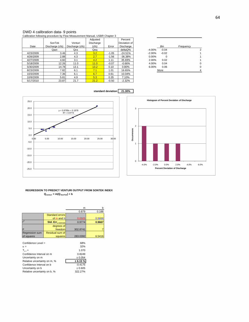
DWD 4 calibration data- 9 pointsCalibration following procedure by Flow Measurement Manual, USBR Chapter 3
DateSonTek
Discharge (cfs)Venturi
Discharge (cfs)
Adjusted Discharge
(cfs) Error
Percent Deviation of Discharge Bin Frequency
Qact Qcs Qeq deltaQ% -4.00% -0.04 24/23/2009 3.46 4.3 3.2 -1.05 -24.51% -2.00% -0.02 14/26/2009 2.88 4.3 2.7 -1.56 -36.38% 0.00% 0 14/27/2009 4.60 3.1 4.2 1.11 35.69% 2.00% 0.02 15/18/2009 12.26 11.0 11.0 -0.07 -0.66% 4.00% 0.04 05/30/2009 14.78 13.1 13.2 0.10 0.80% 6.00% 0.06 08/23/2009 7.82 6.1 7.1 1.01 16.65% More 410/3/2009 7.36 6.1 6.7 0.61 10.04%10/9/2009 5.81 4.9 5.3 0.35 7.10%5/17/2010 23.87 21.7 21.2 -0.50 -2.32%
standard deviation 21.30%
Qventuri = m(Q SonTek) + b
m b0.879 0.188
Standard errors of m and b 0.0505 0.5656
r2 Std. Erry estimate 0.9774 0.9667
Fdegrees of
freedom 302.8741 7Regression sum of squares
Residual sum of squares 283.0392 6.5416
Confidence Level = 68%α = 32%Tα,ν = 1.070Confidence Interval on m 0.8249Uncertainty on m ± 0.054Relative uncertainty on m, % ± 6.15 %Confidence Interval on b -0.4175Uncertainty on b ± 0.605Relative uncertainty on b, % 322.27%
REGRESSION TO PREDICT VENTURI OUTPUT FROM SONTEK INDEX
0
1
2
3
-4.0% -2.0% 0.0% 2.0% 4.0% 6.0%
Occ
urre
nces
Percent Deviation of Discharge
Histogram of Percent Deviation of Discharge
y = 0.8789x + 0.1878R² = 0.9774
-25.0
-20.0
-15.0
-10.0
-5.0
0.0
5.0
10.0
15.0
20.0
25.0
0.00 5.00 10.00 15.00 20.00 25.00 30.00
64

DWD 4 calibration data- 8 pointsCalibration following procedure by Flow Measurement Manual, USBR Chapter 3
DateSonTek
Discharge (cfs)Venturi
Discharge (cfs)
Adjusted Discharge
(cfs) Error
Percent Deviation of Discharge Bin Frequency
Qact Qcs Qeq deltaQ% -4.00% -0.04 34/23/2009 3.46 4.3 3.4 -0.85 -19.88% -2.00% -0.02 14/26/2009 2.88 4.3 3.0 -1.32 -30.86% 0.00% 0 04/27/2009 4.60 3.1 4.4 1.24 39.60% 2.00% 0.02 05/18/2009 12.26 11.0 10.6 -0.46 -4.19% 4.00% 0.04 05/30/2009 14.78 13.1 12.6 -0.45 -3.47% 6.00% 0.06 08/23/2009 7.82 6.1 7.0 0.91 15.12% More 410/3/2009 7.36 6.1 6.6 0.55 9.01%10/9/2009 5.81 4.9 5.3 0.39 7.94%
standard deviation 21.70%
Qventuri = m(Q SonTek) + b
m b0.812 0.617
Standard errors of m and b 0.0874 0.7305
r2 Std. Erry estimate 0.9351 0.9748
Fdegrees of
freedom 86.4062 6Regression sum of squares
Residual sum of squares 82.1086 5.7016
Confidence Level = 68%α = 32%Tα,ν = 1.084Confidence Interval on m 0.7175Uncertainty on m ± 0.095Relative uncertainty on m, % ± 11.66 %Confidence Interval on b -0.1749Uncertainty on b ± 0.792Relative uncertainty on b, % 128.35%
REGRESSION TO PREDICT VENTURI OUTPUT FROM SONTEK INDEX
0
1
2
3
4
-4.0% -2.0% 0.0% 2.0% 4.0% 6.0%
Occ
urre
nces
Percent Deviation of Discharge
Histogram of Percent Deviation of Discharge
y = 0.8122x + 0.6169R² = 0.9351
-20.0
-15.0
-10.0
-5.0
0.0
5.0
10.0
15.0
0.00 2.00 4.00 6.00 8.00 10.00 12.00 14.00 16.00
65

DWD 4 calibration data- 4 pointsCalibration following procedure by Flow Measurement Manual, USBR Chapter 3
DateSonTek
Discharge (cfs)Venturi
Discharge (cfs)
Adjusted Discharge
(cfs) Error
Percent Deviation of Discharge Bin Frequency
Qact Qcs Qeq deltaQ% -4.00% -0.04 24/23/2009 3.46 4.3 3.8 -0.44 -10.40% -2.00% -0.02 14/26/2009 2.88 4.3 3.4 -0.90 -21.05% 0.00% 0 04/27/2009 4.60 3.1 4.7 1.61 51.73% 2.00% 0.02 05/18/2009 12.26 11.0 10.8 -0.27 -2.43% 4.00% 0.04 0
6.00% 0.06 0More 1
standard deviation 32.42%
Qventuri = m(Q SonTek) + b
m b0.788 1.106
Standard errors of m and b 0.1795 1.2436
r2 Std. Erry estimate 0.9060 1.3576
Fdegrees of
freedom 19.2691 2Regression sum of squares
Residual sum of squares 35.5168 3.6864
Confidence Level = 68%α = 32%Tα,ν = 1.312Confidence Interval on m 0.5526Uncertainty on m ± 0.235Relative uncertainty on m, % ± 29.88 %Confidence Interval on b -0.5248Uncertainty on b ± 1.631Relative uncertainty on b, % 147.44%
REGRESSION TO PREDICT VENTURI OUTPUT FROM SONTEK INDEX
0
1
2
3
-4.0% -2.0% 0.0% 2.0% 4.0% 6.0%
Occ
urre
nces
Percent Deviation of Discharge
Histogram of Percent Deviation of Discharge
y = 0.7881x + 1.1062R² = 0.9060
-20.0
-15.0
-10.0
-5.0
0.0
5.0
10.0
15.0
0.00 2.00 4.00 6.00 8.00 10.00 12.00 14.00
66

WWD 5 calibration data- 11 pointsCalibration following procedure by Flow Measurement Manual, USBR Chapter 3
DateSonTek
Discharge (cfs)Venturi
Discharge (cfs)
Adjusted Discharge
(cfs) Error
Percent Deviation of Discharge Bin Frequency
Qact Qcs Qeq deltaQ% -4.00% -0.04 24/26/2009 7.30 7.3 6.9 -0.36 -4.88% -2.00% -0.02 35/15/2009 6.60 6.4 6.3 -0.10 -1.57% 0.00% 0 25/29/2009 16.90 15.6 15.7 0.11 0.70% 2.00% 0.02 15/31/2009 5.77 5.6 5.5 -0.12 -2.14% 4.00% 0.04 08/17/2009 6.43 6.4 6.1 -0.25 -3.92% 6.00% 0.06 18/24/2009 2.48 2.7 2.5 -0.16 -6.03% More 29/14/2009 3.51 3.0 3.4 0.47 15.98%9/25/2009 3.18 3.0 3.1 0.18 5.90%5/8/2010 17.85 16.7 16.6 -0.11 -0.64%5/24/2010 6.76 6.7 6.4 -0.22 -3.33%6/11/2010 9.52 8.4 9.0 0.56 6.60%
standard deviation 6.51%
Qventuri = m(Q SonTek) + b
m b0.917 0.230
Standard errors of m and b 0.0192 0.1776
r2 Std. Erry estimate 0.9961 0.3119
Fdegrees of
freedom 2280.9112 9Regression sum of squares
Residual sum of squares 221.8553 0.8754
Confidence Level = 68%α = 32%Tα,ν = 1.053Confidence Interval on m 0.8969Uncertainty on m ± 0.020Relative uncertainty on m, % ± 2.20 %Confidence Interval on b 0.0428Uncertainty on b ± 0.187Relative uncertainty on b, % 81.37%
REGRESSION TO PREDICT VENTURI OUTPUT FROM SONTEK INDEX
0
1
2
3
4
-4.0% -2.0% 0.0% 2.0% 4.0% 6.0%
Occ
urre
nces
Percent Deviation of Discharge
Histogram of Percent Deviation of Discharge
y = 0.9171x + 0.2297R² = 0.9961
-25.0
-20.0
-15.0
-10.0
-5.0
0.0
5.0
10.0
15.0
20.0
0.00 5.00 10.00 15.00 20.00
67

WWD 5 calibration data- 10 pointsCalibration following procedure by Flow Measurement Manual, USBR Chapter 3
DateSonTek
Discharge (cfs)Venturi
Discharge (cfs)
Adjusted Discharge
(cfs) Error
Percent Deviation of Discharge Bin Frequency
Qact Qcs Qeq deltaQ% -4.00% -0.04 24/26/2009 7.30 7.3 7.0 -0.30 -4.13% -2.00% -0.02 25/15/2009 6.60 6.4 6.3 -0.05 -0.76% 0.00% 0 35/29/2009 16.90 15.6 15.8 0.20 1.29% 2.00% 0.02 15/31/2009 5.77 5.6 5.6 -0.07 -1.29% 4.00% 0.04 08/17/2009 6.43 6.4 6.2 -0.20 -3.13% 6.00% 0.06 08/24/2009 2.48 2.7 2.5 -0.13 -4.71% More 29/14/2009 3.51 3.0 3.5 0.51 17.29%9/25/2009 3.18 3.0 3.2 0.21 7.17%5/8/2010 17.85 16.7 16.7 -0.01 -0.07%5/24/2010 6.76 6.7 6.5 -0.17 -2.54%
standard deviation 6.68%
Qventuri = m(Q SonTek) + b
m b0.921 0.255
Standard errors of m and b 0.0160 0.1473
r2 Std. Erry estimate 0.9976 0.2579
Fdegrees of
freedom 3324.7573 8Regression sum of squares
Residual sum of squares 221.1304 0.5321
Confidence Level = 68%α = 32%Tα,ν = 1.060Confidence Interval on m 0.9041Uncertainty on m ± 0.017Relative uncertainty on m, % ± 1.84 %Confidence Interval on b 0.0989Uncertainty on b ± 0.156Relative uncertainty on b, % 61.23%
REGRESSION TO PREDICT VENTURI OUTPUT FROM SONTEK INDEX
0
1
2
3
4
-4.0% -2.0% 0.0% 2.0% 4.0% 6.0%
Occ
urre
nces
Percent Deviation of Discharge
Histogram of Percent Deviation of Discharge
y = 0.9211x + 0.2550R² = 0.9976
-25.0
-20.0
-15.0
-10.0
-5.0
0.0
5.0
10.0
15.0
20.0
0.00 5.00 10.00 15.00 20.00
68

WWD 5 calibration data- 4 pointsCalibration following procedure by Flow Measurement Manual, USBR Chapter 3
DateSonTek
Discharge (cfs)Venturi
Discharge (cfs)
Adjusted Discharge
(cfs) Error
Percent Deviation of Discharge Bin Frequency
Qact Qcs Qeq deltaQ% -4.00% -0.04 04/26/2009 7.30 7.3 7.1 -0.19 -2.60% -2.00% -0.02 15/15/2009 6.60 6.4 6.5 0.08 1.32% 0.00% 0 05/29/2009 16.90 15.6 15.6 0.02 0.13% 2.00% 0.02 35/31/2009 5.77 5.6 5.7 0.09 1.51% 4.00% 0.04 0
6.00% 0.06 0More 0
standard deviation 1.90%
Qventuri = m(Q SonTek) + b
m b0.891 0.589
Standard errors of m and b 0.0176 0.1798
r2 Std. Erry estimate 0.9992 0.1592
Fdegrees of
freedom 2548.7413 2
Regression sum of squares
Residual sum of squares 64.5945 0.0507
Confidence Level = 68%α = 32%Tα,ν = 1.312Confidence Interval on m 0.8675Uncertainty on m ± 0.023Relative uncertainty on m, % ± 2.60 %Confidence Interval on b 0.3532Uncertainty on b ± 0.236Relative uncertainty on b, % 40.04%
REGRESSION TO PREDICT VENTURI OUTPUT FROM SONTEK INDEX
0
1
2
3
4
-4.0% -2.0% 0.0% 2.0% 4.0% 6.0%
Occ
urre
nces
Percent Deviation of Discharge
Histogram of Percent Deviation of Discharge
y = 0.8906x + 0.5890R² = 0.9992
-20.0
-15.0
-10.0
-5.0
0.0
5.0
10.0
15.0
20.0
0.00 5.00 10.00 15.00 20.00
69

WWD 7 calibration data- 18 pointsCalibration following procedure by Flow Measurement Manual, USBR Chapter 3
DateSonTek
Discharge (cfs)Venturi
Discharge (cfs)
Adjusted Discharge
(cfs) Error
Percent Deviation of Discharge Bin Frequency
Qact Qcs Qeq deltaQ% -4.00% -0.04 34/6/2009 8.1 9.1 7.5 -1.64 -17.98% -2.00% -0.02 1
4/27/2009 8.3 7.3 7.7 0.36 4.96% 0.00% 0 15/11/2009 7.7 7.0 7.1 0.07 1.03% 2.00% 0.02 55/15/2009 21.1 18.8 18.9 0.13 0.68% 4.00% 0.04 45/16/2009 4.9 5.0 4.6 -0.42 -8.43% 6.00% 0.06 25/22/2009 3.2 3.2 3.2 0.03 0.82% More 25/29/2009 5.0 4.2 4.8 0.51 12.08%5/29/2009 12.2 10.8 11.0 0.21 1.90%6/13/2009 6.9 6.3 6.4 0.13 2.04%8/10/2009 6.0 5.9 5.6 -0.28 -4.69%8/21/2009 6.6 5.9 6.2 0.32 5.53%8/24/2009 6.8 5.9 6.3 0.42 7.04%9/14/2009 6.5 5.9 6.0 0.19 3.30%
10/10/2009 9.0 8.1 8.2 0.17 2.06%3/19/2010 11.0 10.3 10.0 -0.33 -3.20%4/16/2010 4.2 4.0 4.0 -0.02 -0.48%5/21/2010 4.2 3.9 4.0 0.09 2.32%6/11/2010 4.5 4.2 4.3 0.06 1.49%
standard deviation 6.43%
Qventuri = m(QSonTek) + b
m b0.879 0.333
Standard errors of m and b 0.0289 0.2476
r2 Std. Erry estimate 0.9830 0.4919
Fdegrees of
freedom 925.5554 16Regression sum of squares
Residual sum of squares 223.9303 3.8711
Confidence Level = 68%α = 32%Tα,ν = 1.026Confidence Interval on m 0.8492Uncertainty on m ± 0.030Relative uncertainty on m, % ± 3.37 %Confidence Interval on b 0.0792Uncertainty on b ± 0.254Relative uncertainty on b, % 76.23%
REGRESSION TO PREDICT VENTURI OUTPUT FROM SONTEK INDEX FLOW MEASUREMENT - Tony Wahl (USBR)
0
1
2
3
4
5
6
-4.0% -2.0% 0.0% 2.0% 4.0% 6.0%
Occ
urre
nces
Percent Deviation of Discharge
Histogram of Percent Deviation of Discharge
y = 0.8789x + 0.3333R² = 0.9830
-20.0
-15.0
-10.0
-5.0
0.0
5.0
10.0
15.0
20.0
25.0
0.0 5.0 10.0 15.0 20.0 25.0
70

WWD 7 calibration data- 10 pointsCalibration following procedure by Flow Measurement Manual, USBR Chapter 3
DateSonTek
Discharge (cfs)Venturi
Discharge (cfs)
Adjusted Discharge
(cfs) Error
Percent Deviation of Discharge Bin Frequency
Qact Qcs Qeq deltaQ% -4.00% -0.04 24/6/2009 8.1 9.1 7.6 -1.54 -16.95% -2.00% -0.02 14/27/2009 8.3 7.3 7.7 0.45 6.21% 0.00% 0 05/11/2009 7.7 7.0 7.2 0.17 2.43% 2.00% 0.02 15/15/2009 21.1 18.8 18.8 0.06 0.33% 4.00% 0.04 35/16/2009 4.9 5.0 4.7 -0.29 -5.78% 6.00% 0.06 15/22/2009 3.2 3.2 3.3 0.18 5.65% More 25/29/2009 5.0 4.2 4.9 0.64 15.16%5/29/2009 12.2 10.8 11.1 0.25 2.30%6/13/2009 6.9 6.3 6.5 0.24 3.75%8/10/2009 6.0 5.9 5.8 -0.16 -2.69%
standard deviation 8.45%
Qventuri = m(Q SonTek) + b
m b0.867 0.525
Standard errors of m and b 0.0418 0.4039
r2 Std. Erry estimate 0.9817 0.6413
Fdegrees of
freedom 429.7075 8Regression sum of squares
Residual sum of squares 176.7447 3.2905
Confidence Level = 68%α = 32%Tα,ν = 1.060Confidence Interval on m 0.8224Uncertainty on m ± 0.044Relative uncertainty on m, % ± 5.11 %Confidence Interval on b 0.0966Uncertainty on b ± 0.428Relative uncertainty on b, % 81.59%
REGRESSION TO PREDICT VENTURI OUTPUT FROM SONTEK INDEX FLOW MEASUREMENT - Tony Wahl (USBR)
0
1
2
3
4
-4.0% -2.0% 0.0% 2.0% 4.0% 6.0%
Occ
urre
nces
Percent Deviation of Discharge
Histogram of Percent Deviation of Discharge
y = 0.8667x + 0.5248R² = 0.9817
-20.0
-15.0
-10.0
-5.0
0.0
5.0
10.0
15.0
20.0
25.0
0.0 5.0 10.0 15.0 20.0 25.0
71

WWD 7 calibration data- 4 pointsCalibration following procedure by Flow Measurement Manual, USBR Chapter 3
DateSonTek
Discharge (cfs)Venturi
Discharge (cfs)
Adjusted Discharge
(cfs) Error
Percent Deviation of Discharge Bin Frequency
Qact Qcs Qeq deltaQ% -4.00% -0.04 14/6/2009 8.1 9.1 7.9 -1.24 -13.61% -2.00% -0.02 04/27/2009 8.3 7.3 8.0 0.75 10.29% 0.00% 0 05/11/2009 7.7 7.0 7.5 0.49 6.90% 2.00% 0.02 15/15/2009 21.1 18.8 18.8 0.00 0.01% 4.00% 0.04 0
6.00% 0.06 0More 2
standard deviation 10.58%
Qventuri = m(Q SonTek) + b
m b0.839 1.056
Standard errors of m and b 0.0953 1.2064
r2 Std. Erry estimate 0.9748 1.0803
Fdegrees of
freedom 77.5033 2Regression sum of squares
Residual sum of squares 90.4490 2.3341
Confidence Level = 68%α = 32%Tα,ν = 1.312Confidence Interval on m 0.7138Uncertainty on m ± 0.125Relative uncertainty on m, % ± 14.90 %Confidence Interval on b -0.5267Uncertainty on b ± 1.582Relative uncertainty on b, % 149.89%
REGRESSION TO PREDICT VENTURI OUTPUT FROM SONTEK INDEX
0
1
2
-4.0% -2.0% 0.0% 2.0% 4.0% 6.0%
Occ
urre
nces
Percent Deviation of Discharge
Histogram of Percent Deviation of Discharge
y = 0.8388x + 1.0556R² = 0.9748
-15.0
-10.0
-5.0
0.0
5.0
10.0
15.0
20.0
25.0
0.0 5.0 10.0 15.0 20.0 25.0
72

WWD 8 calibration data- 14 pointsCalibration following procedure by Flow Measurement Manual, USBR Chapter 3
DateSonTek
Discharge (cfs)Venturi
Discharge (cfs)
Adjusted Discharge
(cfs) Error
Percent Deviation of Discharge Bin Frequency
Qact Qcs Qeq deltaQ% -4.00% -0.04 45/15/2009 3.9 4.2 3.9 -0.31 -7.43% -2.00% -0.02 35/17/2009 5.8 6.0 6.0 -0.01 -0.20% 0.00% 0 25/22/2009 8.0 8.6 8.4 -0.28 -3.28% 2.00% 0.02 05/29/2009 8.1 8.9 8.5 -0.37 -4.12% 4.00% 0.04 15/30/2009 7.5 8.1 7.9 -0.22 -2.78% 6.00% 0.06 16/13/2009 11.2 12.1 12.0 -0.12 -1.01% More 38/9/2009 2.0 2.0 1.8 -0.17 -8.58%
8/10/2009 2.2 2.4 2.0 -0.37 -15.30%8/14/2009 9.6 9.8 10.1 0.31 3.17%9/12/2009 5.1 4.5 5.2 0.68 15.10%10/1/2009 5.5 5.2 5.6 0.39 7.46%
10/10/2009 4.2 4.3 4.2 -0.12 -2.77%4/16/2010 4.5 4.2 4.5 0.36 8.50%4/23/2010 4.3 4.1 4.3 0.24 5.82%
standard deviation 7.87%
Qventuri = m(QSonTek) + b
m b1.099 -0.382
Standard errors of m and b 0.0357 0.2284
r2 Std. Erry estimate 0.9875 0.3485
Fdegrees of
freedom 945.9738 12Regression sum of squares
Residual sum of squares 114.9174 1.4578
Confidence Level = 68%α = 32%Tα,ν = 1.037Confidence Interval on m 1.0618Uncertainty on m ± 0.037Relative uncertainty on m, % ± 3.37 %Confidence Interval on b -0.6186Uncertainty on b ± 0.237Relative uncertainty on b, % -62.10%
REGRESSION TO PREDICT VENTURI OUTPUT FROM SONTEK INDEX FLOW MEASUREMENT - Tony Wahl (USBR)
0
1
2
3
4
5
-4.0% -2.0% 0.0% 2.0% 4.0% 6.0%
Occ
urre
nces
Percent Deviation of Discharge
Histogram of Percent Deviation of Discharge
y = 1.0988x - 0.3816R² = 0.9875
-30.0
-25.0
-20.0
-15.0
-10.0
-5.0
0.0
5.0
10.0
15.0
0.0 2.0 4.0 6.0 8.0 10.0 12.0
73
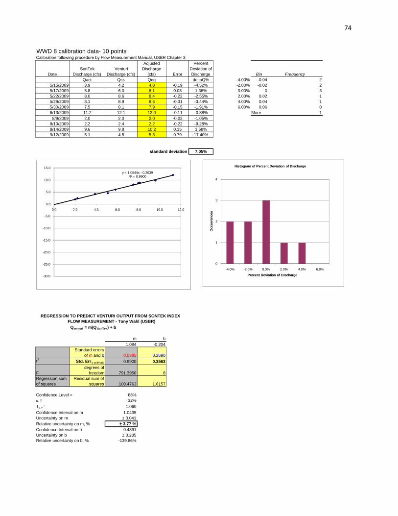
WWD 8 calibration data- 10 pointsCalibration following procedure by Flow Measurement Manual, USBR Chapter 3
DateSonTek
Discharge (cfs)Venturi
Discharge (cfs)
Adjusted Discharge
(cfs) Error
Percent Deviation of Discharge Bin Frequency
Qact Qcs Qeq deltaQ% -4.00% -0.04 25/15/2009 3.9 4.2 4.0 -0.19 -4.52% -2.00% -0.02 25/17/2009 5.8 6.0 6.1 0.08 1.36% 0.00% 0 35/22/2009 8.0 8.6 8.4 -0.22 -2.55% 2.00% 0.02 15/29/2009 8.1 8.9 8.6 -0.31 -3.44% 4.00% 0.04 15/30/2009 7.5 8.1 7.9 -0.15 -1.91% 6.00% 0.06 06/13/2009 11.2 12.1 12.0 -0.11 -0.88% More 18/9/2009 2.0 2.0 2.0 -0.02 -1.05%
8/10/2009 2.2 2.4 2.2 -0.22 -9.28%8/14/2009 9.6 9.8 10.2 0.35 3.58%9/12/2009 5.1 4.5 5.3 0.79 17.40%
standard deviation 7.05%
Qventuri = m(Q SonTek) + b
m b1.084 -0.204
Standard errors of m and b 0.0385 0.2690
r2 Std. Erry estimate 0.9900 0.3563
Fdegrees of
freedom 791.3950 8Regression sum of squares
Residual sum of squares 100.4763 1.0157
Confidence Level = 68%α = 32%Tα,ν = 1.060Confidence Interval on m 1.0435Uncertainty on m ± 0.041Relative uncertainty on m, % ± 3.77 %Confidence Interval on b -0.4891Uncertainty on b ± 0.285Relative uncertainty on b, % -139.86%
REGRESSION TO PREDICT VENTURI OUTPUT FROM SONTEK INDEX FLOW MEASUREMENT - Tony Wahl (USBR)
0
1
2
3
4
-4.0% -2.0% 0.0% 2.0% 4.0% 6.0%
Occ
urre
nces
Percent Deviation of Discharge
Histogram of Percent Deviation of Discharge
y = 1.0844x - 0.2039R² = 0.9900
-30.0
-25.0
-20.0
-15.0
-10.0
-5.0
0.0
5.0
10.0
15.0
0.0 2.0 4.0 6.0 8.0 10.0 12.0
74

WWD 8 calibration data- 4 pointsCalibration following procedure by Flow Measurement Manual, USBR Chapter 3
DateSonTek
Discharge (cfs)Venturi
Discharge (cfs)
Adjusted Discharge
(cfs) Error
Percent Deviation of Discharge Bin Frequency
Qact Qcs Qeq deltaQ% -4.00% -0.04 05/15/2009 3.9 4.2 4.1 -0.12 -2.83% -2.00% -0.02 15/17/2009 5.8 6.0 6.2 0.22 3.64% 0.00% 0 25/22/2009 8.0 8.6 8.6 -0.01 -0.12% 2.00% 0.02 05/29/2009 8.1 8.9 8.8 -0.09 -1.01% 4.00% 0.04 1
6.00% 0.06 0More 0
standard deviation 2.73%
Qventuri = m(Q SonTek) + b
m b1.119 -0.265
Standard errors of m and b 0.0540 0.3599
r2 Std. Erry estimate 0.9954 0.1873
Fdegrees of
freedom 429.0765 2Regression sum of squares
Residual sum of squares 15.0495 0.0701
Confidence Level = 68%α = 32%Tα,ν = 1.312Confidence Interval on m 1.0478Uncertainty on m ± 0.071Relative uncertainty on m, % ± 6.33 %Confidence Interval on b -0.7375Uncertainty on b ± 0.472Relative uncertainty on b, % -177.79%
REGRESSION TO PREDICT VENTURI OUTPUT FROM SONTEK INDEX
0
1
2
3
-4.0% -2.0% 0.0% 2.0% 4.0% 6.0%
Occ
urre
nces
Percent Deviation of Discharge
Histogram of Percent Deviation of Discharge
y = 1.1186x - 0.2655R² = 0.9954
-25.0
-20.0
-15.0
-10.0
-5.0
0.0
5.0
10.0
15.0
0.0 2.0 4.0 6.0 8.0 10.0
75

WWD 9B-3 calibration data- 12 pointsCalibration following procedure by Flow Measurement Manual, USBR Chapter 3
DateSonTek
Discharge (cfs)Venturi
Discharge (cfs)
Adjusted Discharge
(cfs) Error
Percent Deviation of Discharge Bin Frequency
Qact Qcs Qeq deltaQ% -4.00% -0.04 44/27/2009 2.9 3.3 2.8 -0.51 -15.25% -2.00% -0.02 25/17/2009 2.8 2.8 2.8 0.03 0.97% 0.00% 0 05/22/2009 2.9 2.4 2.9 0.50 21.46% 2.00% 0.02 25/29/2009 5.7 5.8 5.5 -0.23 -4.06% 4.00% 0.04 05/31/2009 2.7 3.0 2.7 -0.31 -10.49% 6.00% 0.06 06/13/2009 2.9 3.1 2.9 -0.21 -6.72% More 49/14/2009 5.9 5.9 5.7 -0.22 -3.69%9/25/2009 2.8 2.4 2.7 0.37 15.71%10/1/2009 8.5 8.4 8.2 -0.18 -2.17%3/19/2010 5.7 5.4 5.5 0.08 1.41%3/25/2010 5.9 5.4 5.8 0.34 6.27%4/18/2010 5.9 5.4 5.8 0.34 6.27%
standard deviation 10.46%
Qventuri = m(Q SonTek) + b
m b0.956 0.084
Standard errors of m and b 0.0529 0.2595
r2 Std. Erry estimate 0.9703 0.3404
Fdegrees of
freedom 326.6306 10Regression sum of squares
Residual sum of squares 37.8414 1.1585
Confidence Level = 68%α = 32%Tα,ν = 1.046Confidence Interval on m 0.9005Uncertainty on m ± 0.055Relative uncertainty on m, % ± 5.79 %Confidence Interval on b -0.1874Uncertainty on b ± 0.272Relative uncertainty on b, % 322.77%
REGRESSION TO PREDICT VENTURI OUTPUT FROM SONTEK INDEX FLOW MEASUREMENT - Tony Wahl (USBR)
0
1
2
3
4
5
-4.0% -2.0% 0.0% 2.0% 4.0% 6.0%
Occ
urre
nces
Percent Deviation of Discharge
Histogram of Percent Deviation of Discharge
y = 0.9559x + 0.0841R² = 0.9703
-25.0
-20.0
-15.0
-10.0
-5.0
0.0
5.0
10.0
0.0 2.0 4.0 6.0 8.0 10.0
76

WWD 9B-3 calibration data- 10 pointsCalibration following procedure by Flow Measurement Manual, USBR Chapter 3
DateSonTek
Discharge (cfs)Venturi
Discharge (cfs)
Adjusted Discharge
(cfs) Error
Percent Deviation of Discharge Bin Frequency
Qact Qcs Qeq deltaQ% -4.00% -0.04 34/27/2009 2.9 3.3 2.8 -0.48 -14.51% -2.00% -0.02 15/17/2009 2.8 2.8 2.8 0.05 1.82% 0.00% 0 15/22/2009 2.9 2.4 2.9 0.53 22.55% 2.00% 0.02 25/29/2009 5.7 5.8 5.6 -0.12 -2.11% 4.00% 0.04 15/31/2009 2.7 3.0 2.7 -0.29 -9.84% 6.00% 0.06 06/13/2009 2.9 3.1 2.9 -0.18 -5.88% More 29/14/2009 5.9 5.9 5.8 -0.10 -1.69%9/25/2009 2.8 2.4 2.7 0.39 16.62%10/1/2009 8.5 8.4 8.4 0.02 0.20%3/19/2010 5.7 5.4 5.6 0.19 3.46%
standard deviation 11.25%
Qventuri = m(Q SonTek) + b
m b0.987 0.020
Standard errors of m and b 0.0537 0.2507
r2 Std. Erry estimate 0.9769 0.3252
Fdegrees of
freedom 338.2114 8Regression sum of squares
Residual sum of squares 35.7737 0.8462
Confidence Level = 68%α = 32%Tα,ν = 1.060Confidence Interval on m 0.9300Uncertainty on m ± 0.057Relative uncertainty on m, % ± 5.77 %Confidence Interval on b -0.2459Uncertainty on b ± 0.266Relative uncertainty on b, % 1335.54%
REGRESSION TO PREDICT VENTURI OUTPUT FROM SONTEK INDEX FLOW MEASUREMENT - Tony Wahl (USBR)
0
1
2
3
4
-4.0% -2.0% 0.0% 2.0% 4.0% 6.0%
Occ
urre
nces
Percent Deviation of Discharge
Histogram of Percent Deviation of Discharge
y = 0.9869x + 0.0199R² = 0.9769
-25.0
-20.0
-15.0
-10.0
-5.0
0.0
5.0
10.0
0.0 2.0 4.0 6.0 8.0 10.0
77

WWD 9B-3 calibration data- 4 pointsCalibration following procedure by Flow Measurement Manual, USBR Chapter 3
DateSonTek
Discharge (cfs)Venturi
Discharge (cfs)
Adjusted Discharge
(cfs) Error
Percent Deviation of Discharge Bin Frequency
Qact Qcs Qeq deltaQ% -4.00% -0.04 14/27/2009 2.9 3.3 2.8 -0.51 -15.44% -2.00% -0.02 05/17/2009 2.8 2.8 2.8 0.02 0.66% 0.00% 0 15/22/2009 2.9 2.4 2.9 0.50 21.34% 2.00% 0.02 15/29/2009 5.7 5.8 5.7 -0.01 -0.13% 4.00% 0.04 0
6.00% 0.06 0More 1
standard deviation 15.10%
Qventuri = m(Q SonTek) + b
m b1.038 -0.157
Standard errors of m and b 0.2075 0.7821
r2 Std. Erry estimate 0.9260 0.5072
Fdegrees of
freedom 25.0397 2Regression sum of squares
Residual sum of squares 6.4423 0.5146
Confidence Level = 68%α = 32%Tα,ν = 1.312Confidence Interval on m 0.7660Uncertainty on m ± 0.272Relative uncertainty on m, % ± 26.21 %Confidence Interval on b -1.1826Uncertainty on b ± 1.026Relative uncertainty on b, % -653.75%
REGRESSION TO PREDICT VENTURI OUTPUT FROM SONTEK INDEX
0
1
2
-4.0% -2.0% 0.0% 2.0% 4.0% 6.0%
Occ
urre
nces
Percent Deviation of Discharge
Histogram of Percent Deviation of Discharge
y = 1.0381x - 0.1569R² = 0.9260
-25.0
-20.0
-15.0
-10.0
-5.0
0.0
5.0
10.0
0.0 1.0 2.0 3.0 4.0 5.0 6.0
78

79
APPENDIX C
TCCA Venturi Calibration

80
The calibration of the SonTek Argonaut-SW flow meters will be completed by Tehema-Colusa Canal Authority (TCCA). The purpose of the procedures is to assist in collecting data to be used to properly calibrate the SonTek Argonaut-SW flow meters. Tehema-Colusa Canal Authority is responsible for:
• Calibrating the Venturi • Making head measurement checks on the venturi • Recording data from both the venturi and the SonTek flow meters during head
test • Informing DEID when the head measurement check is complete
Procedures The procedure for calibration includes head measurement checks on the venturi, meter reading and turning off of pumps, and calibration post-processing completed by ITRC. Tehema-Colusa Canal Authority The procedures for TCCA’s responsibilities are outlined below: Step 1. The flow rate needs to be stable when taking a calibration point.
Step 2. Complete a standard head test on the venturi. The head test measurement method
utilizes an air-water manometer to measure the pressure differential through the venturi. Using the air-manometer method, the difference in head across the venturi is found by measuring the height difference between the two water levels in a ½” diameter clear tube. The tubing of the air-water manometer is attached to the wall in the access shaft. Before the head is measured, water is bled from the venturi to make sure no air is in the lines as seen in Figure 10. The height of water in the tube is measured with a tape measure.
Figure 48 Venturi line being bled of air
Step 3. Record basic data from the SonTek recorder on the data sheet. Figure 11 shows the screen from the SonTek display that shows the basic data to be recorded. The SonTek has multiple screens that can be scrolled through using the yellow “next screen” button. Record the SonTek date, time, and flow rate.

81
Figure 49 SonTek Flow Display
Step 4. Record the Badger flow rate. Figure 12 shows the Badger and the screen has a red
oval around it.
Figure 50 Badger Flow Display
Step 5. Make sure to note if the pumps are on at the site. If the pumps are on, the venturi and SonTek may not agree with each other depending on the set up of the site.