Evaluation of applicability of numerical modelling tools for complex slope stability problems in

Hokkaido

Graduate School of Engineering, Hokkaido University, Student Member, (○) Srikrishnan SIVA SUBRAMANIAN

Faculty of Engineering, Hokkaido University, International Member, Tatsuya ISHIKAWA

Tomakomai National College of Technology, International Member, Tetsuya TOKORO

1 Introduction

Slope stability against anticipated earthquake vibrations is an engineering issue in earthquake prone regions like Hokkaido. Due to

repeated earthquake ground vibrations the soil losses its shear strength and slope failure occurs. Hokkaido, being a cold region

experiences varied amount of rainfall and freeze and thaw cycles every year. This affects the slope stability and it affects the shear

strength of the soil which is very complex to understand (Kawamura and Miura, 2013). The stability of a soil slope in the event of an

earthquake also depends on its stability in static state (Terzaghi, 1950). When the slopes are close to static failure small seismic shocks

may be enough to trigger a collapse. This study involves analysis of seismic stability and simulation of seismic behaviour of soil

slopes using different numerical modelling approaches. The numerical analysis in this study is performed using GeoStudio finite

element software (FEM) (GEO-SLOPE International, Ltd., 2012) and FLAC2D Fast Lagrangian Analysis of Continua finite difference

software (FDM) (Itasca, 2012). The soil slopes are simulated against various peak ground accelerations (PGA) and dynamic factor of

safety is evaluated for the entire earthquake duration. The results are obtained in the form of failure surface and dynamic factor of

safety fluctuation over time.

2 Modelling methodology and experimental considerations

The aim of this study is to evaluate the applicability of numerical modelling tools to analyse dynamic slope stability problems. It

should be kept in consideration that the dynamic characteristics of geomaterials are precisely analysed using laboratory experiments i.e.

shaking table tests, geotechnical centrifuge etc. This study attempts to simulate the shaking table test environment in numerical

modelling tools from which the results of laboratory experiments can be cross verified and validated. For this purpose the numerical

modelling has been performed with experimental setup pertaining to model shaking table tests. The dynamic numerical modelling in this study has been performed in three stages as given below.

1. Slope stability analysis and modelling of soil slope in static state,

2. Slope stability analysis and modelling of soil slope in dynamic state,

3. Simulations of shaking table model with PWP build up due to earthquake.

The slope geometry for numerical simulations has been configured in consideration to the shaking table tests. The slope geometry for

numerical simulations designed with assumed parameters is as given in Figure 1.

Figure 1 Slope geometry adopted for numerical simulations

Evaluation of applicability of numerical modelling tools for complex slope stability problems in Hokkaido. Srikrishnan SIVA

SUBRAMANIAN (Hokkaido University), Tatsuya ISHIKAWA (Hokkaido University), Tetsuya TOKORO (Tomakomai

National College of Technology).

地盤工学会 北海道支部

技術報告集 第 5 5 号

平成27年1月 於 室 蘭 市

215

Toyoura Sand has been used in model soil slopes of the shaking table. The shear strength properties of Toyoura Sand have been

obtained from previous laboratory test results (Ozaki, 2004) and (Miura and Yagi 2003). The angle of internal friction of Toyoura sand

has been considered as 40° based on triaxial compression tests performed by Ozaki (2004) corresponding to 40% relative density. The

E-Modulus is given as 300MPa based on the test results. The cohesion of the soil is kept as 0 due to assumed loose state of the sand in

shaking table.

Table 1 Soil parameters for numerical simulations

e - Void Ratio emax emin Dr(%)

Dry

Density

ρd (g/cm3)

Gs

(g/cm3)

Unit

weight

(kN/m3)

Young’s

modulus

(kPa)

Poisson’s ratio

Damping ratio

Cohesion (kPa)

Angle

of

internal friction

0.82 0.96 0.61 40 1.26 2.64 1.26E+01 300,000 0.334 0.05 0 40°

The analytical conditions for the model shaking table tests were predetermined and numerical modelling has been performed in a

similar manner of shaking table tests so as to enable validation of the numerical results with shaking table tests. The assumed soil parameters of the soil slope in model shaking table tests are as given in Table 1.

3 Modelling using GeoStudio

Dynamic numerical modelling has been performed using three components SIGMA/W, QUAKE/W and SLOPE/W, in a complete

suite of geotechnical products called GeoStudio (John Krahn 2004). SIGMA/W is a finite element stress analysis tool used for static

analysis. QUAKE/W is a finite element dynamic analysis tool. SLOPE/W is a slope stability analysis tool based on the method of

slices. Dynamic analyses are carried over using QUAKE/W to compute the dynamic stress conditions and are keyed in to SLOPE/W to

compute the factor of safety. During the analysis the FEM nodes keep records of information about the stresses. During dynamic

analysis the nodes will contain dynamic stresses and static stresses. The relationship between the dynamic and static stresses is given by equation 1. The dynamic stresses are evaluated in QUAKE/W using the following equation,

………….. (1)

here σdynamic is dynamic stress, σ static is static stress and σ is the total stress (static+dynamic) acting at a point.

The dynamic stresses are computed at the base of each slice. Integrating along the entire slip surface then gives the total dynamic

mobilized shear stress. This is the additional shear stress created by the earthquake shaking. Once the mobilized and resisting shear

stresses are available for each slice, the forces can be integrated over the length of the slip surface to determine the stability factor. The factor of safety (F.O.S) is defined as,

………….. (2)

where Sr is the total available shear resistance and Sm is the total mobilized shear stress along the entire length of the slip surface. The modelling methodology adopted in GeoStudio is given in Figure 2.

Figure 2 Modelling methodology adopted in GeoStudio

3.1 Static simulation of soil slope

Prior evaluating the dynamic stability of soil slope it will be prudent to analyse its stability in static state. To perform static slope

stability analysis a component of GeoStudio SIGMA/W has been used to evaluate the stress state of the slope through finite element

method. The slope geometry and soil strength properties have been keyed into the tool with applying roller boundaries at horizontal(x)

and vertical directions(y). The boundaries applied at the slope bottom and sides are as given in Figure 1. The stress state derived from

SIGMA/W analysis has been carried over to SLOPE/W in order to estimate a factor of safety. The static stresses at the base of each

slice have been estimated and integrated along the entire slice gives the total static shear stress. The safety factor of slope has been

estimated using equation 2. The static safety factor of the soil slope estimated using FEM is 1.562. The minimum optimised failure surface and factor of safety have been given in Figure 3.

3.2 Dynamic simulation of soil slope

Dynamic simulations have been performed using QUAKE/W. The soil slope has been modeled and solved in initial static state using

SIGMA/W (insitu state) in order to bring the model into equilibrium. Once the static analysis is over, horizontal and vertical

earthquake wave motions have been keyed in and dynamic deformation analysis is performed. Dynamic stress levels for maximum and

216

minimum earthquake accelerations have been computed and then keyed into SLOPE/W to compute a factor of safety. Equation 1 explains the way dynamic stresses are estimated in QUAKE/W. The factor of safety has been estimated using Equation 2.

Figure 3 Failure surface and factor of safety of soil slope in static state (FEM)

The soil slope has been simulated against various earthquake accelerations and frequencies. To analyse the soil slope in Level 1

earthquake vibration 1995 Kobe earthquake motion has been used in this study. Figure 4 shows the typical seismic waveforms used in

GeoStudio.

Figure 4 (a) Sinusoidal waveform with 100 Gal PGA at 1 Hz frequency (b) Sinusoidal waveform with 100 Gal PGA at 1 Hz frequency (c)

Earthquake acceleration record of 1995 Great Hanshin Earthquake (N-S component)

3.2.1 Effect of increasing peak ground accelerations

The soil slope has been simulated against PGAs ranging from 100 Gal to 500 Gal with fixed frequencies. The frequencies adopted for

this study ranges from 1 Hz to 3 Hz. To analyse the effect of increasing PGAs the slope has been simulated using 100 Gal, 200 Gal, 300 Gal, 400 Gal and 500 Gal with a fixed frequency 1 Hz.

Figure 5 Dynamic factor of safety vs. time (a) PGA 100 Gal (b) PGA 200 Gal (c) PGA 300 Gal (d) PGA 400 Gal (e) PGA 500 Gal

(f) Effect of increasing PGA on slope stability

Figures 5 a, b, c, d and e show the variation of factor of safety over time for PGAs 100 Gal, 200 Gal, 300 Gal, 400 Gal and 500 Gal

respectively. It can be observed that the safety factor of the slope decreases with increasing PGA and the slope completely fails for

PGA >400 Gal. The safety factor values for increasing PGAs are plotted with static factor of safety and given in Figure 5 (f). The soil

217

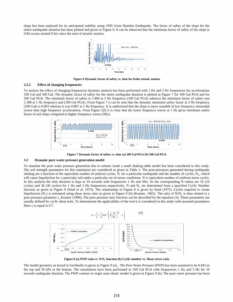
slope has been analysed for its anticipated stability using 1995 Great Hanshin Earthquake. The factor of safety of the slope for the

entire earthquake duration has been plotted and given in Figure 6. It can be observed that the minimum factor of safety of the slope is 0.84 occurs around 8 Sec since the start of seismic motion.

Figure 6 Dynamic factor of safety vs. time for Kobe seismic motion

3.2.2 Effect of changing frequencies

To analyse the effect of changing frequencies dynamic analysis has been performed with 1 Hz and 3 Hz frequencies for accelerations

100 Gal and 500 Gal. The dynamic factor of safety for the entire earthquake duration is plotted in Figure 7 for 100 Gal PGA and for

500 Gal PGA. The minimum factor of safety is 1.469 at 3 Hz frequency (100 Gal PGA) whereas the minimum factor of safety was

1.398 at 1 Hz frequency and (100 Gal PGA). From Figure 7 it can be seen that the dynamic minimum safety factor at 3 Hz frequency

(500 Gal) is 0.893 whereas it was 0.867 at 1 Hz frequency. It is understood that the slope is more unstable in low frequency sinusoidal

waves than high frequency accelerations. From Figure 5(f) it is clear that the lower frequency waves at 1 Hz gives minimum safety factor of soil slope compared to higher frequency waves (3Hz).

Figure 7 Dynamic factor of safety vs. time (a) 100 Gal PGA (b) 500 Gal PGA

3.3 Dynamic pore water pressure generation model

To simulate the pore water pressure generation due to seismic loads a small shaking table model has been considered in this study.

The soil strength parameters for this simulation are considered as given in Table 1. The pore-pressures generated during earthquake

shaking are a function of the equivalent number of uniform cycles, N, for a particular earthquake and the number of cycles, NL, which

will cause liquefaction for a particular soil under a particular set of stress conditions. N is equivalent number of uniform stress cycles.

In this analysis the time duration is kept as 10 seconds with frequencies 1 Hz and 3Hz. So the corresponding N values are 10 (10

cycles) and 30 (30 cycles) for 1 Hz and 3 Hz frequencies respectively. N and NL are determined from a specified Cyclic Number

function as given in Figure 8 (Seed et al. 1975). The relationship in Figure 8 is given by Seed (1975) .Cycles required to create

liquefaction (NL) is estimated using shear stress ratio as given in Figure 8 (b) (Kramer, 1965). The ratio of N/NL is then related to a

pore pressure parameter ru Kramer (1996). The pore pressure ratio function can be described by the equation (3). These parameters are

usually defined by cyclic shear tests. To demonstrate the applicability of the tool it is considered in this study with assumed parameters.

Hereαis equal to 0.7.

1

N

N2Sin

π

1

2

1r

α1

L

1u

(3)

Figure 8 (a) PWP ratio vs. N/NL function (b) Cyclic number vs. Shear stress ratio

The model geometry as keyed in GeoStudio is given in Figure 9 (a).. The Pore Water Pressure (PWP) has been assumed to be 0 kPa in

the top and 30 kPa in the bottom. The simulations have been performed in 100 Gal PGA with frequencies 1 Hz and 3 Hz for 10

seconds earthquake duration. The PWP contour in virgin state elastic model is given in Figure 9 (b). The pore water pressure has been

218

monitored in two points at the bottom of the model during seismic loadings. The model initially had been solved in insitu stress state

and after obtaining static equilibrium conditions seismic loadings have been given in horizontal and vertical directions. The PWP

increase for different PGAs and frequencies using sinusoidal wave is given in Figure 9 (c). From Figure 9(c) it can be observed that the PWP increases up to 3 kPa in Point 2 (Bottom) and around 2.5 kPa at Point 1.

Figure 9 (a) Shaking table model in QUAKE/W (b) PWP contours (kPa) in virgin state elastic model (c) PWP increase due to earthquake for

100 Gal PGA with different frequencies

The PWP initially increases up to 2.5 kPa in Point 1, 3 kPa in Point 2 and remains constant until the end of earthquake. This may be

due the sinusoidal waveforms considered in this study. The PWP increase (liquefaction) occurs within 2 seconds of seismic loading

based on the configurations in this model. After 2 seconds the PWP held constant until the loading ends. The frequencies of the

waveform used here is 1 Hz and 3 Hz. It can be observed that the PWP increase varies among frequencies. In Point 1 the PWP

increases gradually for 1 Hz frequency whereas it increases suddenly for 3 hz frequency. Point 2 also shows the same tendency.

Anyhow it is difficult to demonstrate the effect of frequency with this model due to the fact that assumed parameters are not properly

defined. The N and NL values should be decided based on the earthquake magnitude (Seed et al. (1975). In this example sinusoidal

wave of 100 Gal PGA is only used. Also the model should be tested with real seismic inputs provided with cyclic shear test results.

For proper simulation of PWP using these tool further studies will be performed along with laboratory testing. Nabili et al (2008) have

used GeoStudio to simulate the PWP due to seismic loads. The pore water pressure increase for any anticipated earthquake

acceleration can be estimated using this tool. This model suggests the applicability of GeoStudio to simulate liquefaction due to earthquakes.

4 Modelling using FLAC2D

Numerical modelling has been carried over in FLAC2D to compare the results obtained from SLOPE/W. FLAC2D is a two

dimensional numerical tool for soil and rock modelling based on Finite Difference Method (FDM). Static slope stability analysis of the

soil slope is performed followed by the dynamic analysis. Mohr – Coulomb elasto plastic material model has been adopted for both

static and dynamic analysis. Factor of safety of the soil slope in static state is estimated using built-in Shear Strength Reduction (SSR)

technique. A built in model to simulate the excess pore pressure build up due to seismic load has been used and its applicability has been discussed. Numerical modelling in FLAC2D had been performed through the following stages

Stage 1: Virgin model loaded with slope geometry, boundary conditions and insitu state of stresses etc.

Stage 2: Cycling the model in elastic stage to reach static equilibrium

Stage 3: Mohr-Coulomb elasto plastic analysis and estimation of factor of safety using Shear Strength Reduction (SSR) technique.

Stage 4: Dynamic analysis with sinusoidal waves for different accelerations and frequencies.

4.1 Static slope stability analysis using FLAC2D

Figure 10 FLAC2D grid used for numerical simulations

219

The slope geometry for FLAC analysis is same as the soil slope model used in SLOPE/W. The slope geometry has been built in FLAC

and as given in Figure 10. The material properties used in FLAC simulation are as given in Table 1. The model has been cycled to

reach its equilibrium state in elastic analysis. The vertical stress contours after elastic run of the soil slope is given in Figure 11 (a).

Mohr-coulomb elasto plastic analysis is performed in continuation to the elastic analysis. The failure zones of the slope using elasto

plastic analysis is as given in Figure 11 (b). From Figure 11 (b) it can be seen that only the skin of the slope has been yielded in static state.

Figure 11 (a) Vertical stress contours of the soil slope. (b) Mohr-Coulomb elasto plastic simulation of soil slope

4.2 Shear strength reduction technique

The strength reduction method for determining factor of safety is implemented in FLAC based on Mohr-Coulomb elasto-plastic

material model using the bracketing approach. To perform slope-stability analysis with the shear-reduction technique actual shear-

strength properties cohesion (c) and friction angle (φ) are reduced according to the following equations,

C trial = C (1/F) (4)

φ trial = arctan {(1/F) tan φ} (5)

where c = cohesion, φ = friction angle and F = factor of safety.

A series of simulations are made using trial values of the factor Ftrial to reduce the cohesion, c, and friction angle, φ, until slope failure

occurs. In this study the cohesion is considered as 0. So the simulation to find the weakest plane on the slope is done by Ftrial and φ trial

using equation 5. A bracketing approach is used to solve the model (Dawson and Roth 1999). Unlike conventional limit-equilibrium

stability analyses based on the method of slices, the shear strength reduction technique has a number of advantages (Dawson and Roth

1999). In the above technique incorporated in FLAC it is not necessary to specify the shape of the failure surface in advance, as the

critical failure surface (or multiple failure surfaces) evolves automatically through the weakest zone during the solution. The failure

surface and factor of safety estimated using SSR method is given in Figure 13. The safety factor of the slope is 1.44 in static state. It

should be noted that the safety factor is less compared to the static safety factor obtained through FEM analysis using equal number of

slices. The area of the failure surface in Figure 12 is approximately 38 cm2 whereas it was 48cm2 in the failure surface obtained by

SLOPE/W in Figure 3.

Figure 12 Factor of safety and failure surface estimated using SSR method

4.3 Dynamic simulations using FLAC2D

Dynamic simulations have been performed using built-in dynamic option of FLAC2D. The interpretation and post processing of data

has been performed using FISH a built in language of FLAC. The earthquake waves are simulated at a depth of 1m below the slope toe.

These waves are considered as sine waves which travel in upward direction with the local damping of 3.5-5.0%. The dynamic analysis

is been carried out considering the motion of seismic (sinusoidal) wave in X (horizontal) and Z (vertical) directions with different peak

accelerations of seismic (sinusoidal) wave.

………….. (6)

where Accparticle is acceleration of the particles, ACCP is peak acceleration of wave, t is dynamic time of the wave, ω is angular velocity of wave.

………….. (7)

220

here f is frequency of oscillation of wave.

4.3.1 Procedure for dynamic mechanical simulations

A static equilibrium calculation always precedes a dynamic analysis. There are generally four components to the dynamic analysis

stage:

1. Ensure that model conditions satisfy the requirements for accurate wave transmission.

2. Specify appropriate mechanical damping, representative of the problem materials and input frequency range.

3. Apply dynamic loading and boundary conditions. 4. Set up histories to monitor the dynamic response of the model.

4.3.2 Effect of increasing peak ground accelerations

To analyse the effect of increasing PGA the soil slope has been simulated against 100 Gal, 200 Gal, 300 Gal, 400 Gal and 500 Gal

PGAs. The earthquake response is monitored in slope top. The duration of the earthquake motion is 10 Seconds. The maximum

response acceleration for each PGA has been recorded at the slope top and plotted in Figure 13 (a).

Figure 13 (a) Maximum acceleration response at slope against PGAs, (b) Maximum displacement against PGAs

Figure 13 (b) shows the maximum displacement of the slope for increasing PGAs. From Figure 14 (a) and (b) it can be observed that

the stability of the slope decreases as the input acceleration increases. The slope reaches its maximum acceleration and displacement

for 400 Gal acceleration input and completely fails at 500 Gal PGA. To visualise the effect of increasing PGAs the Mohr-Coulomb elasto plastic failure zones have been plotted in Figure 14.

Figure 14 Elasto-plastic failure zones of the slope against increasing PGAs

From Figure 14 it can be observed that the failure zones increase with the input acceleration and complete slope failure occurs for

PGAs > 400 Gal. The results are similar to the results obtained from GeoStudio simulations.

4.3.3 Effect of changing frequencies

Figure 15 Effect of changing frequencies in earthquake response of slope (a) Frequency vs. PGA (b) Frequency vs. Maximum displacement

To analyse the effect of frequencies sinusoidal waveforms of 1 Hz and 3 Hz have been used with 100 Gal PGA. The slope acceleration

response had been monitored during the simulation. The results are plotted in Figure 15. It is interesting to note the variation in

221

response acceleration and maximum displacement for different frequencies. It can be inferred that at low frequency earthquake the

slope failure tendency is high as compared to higher frequencies. From Figure 15 (a) and (b) it can be seen that the acceleration

response and maximum displacement is high for frequency 1 Hz as compared with frequencies 2 Hz and 3 Hz. Similar results are obtained from QUAKE/W modelling.

4.4 Dynamic pore pressure generation model

To simulate the excess pore water pressure due to seismic loads a built-in model of FLAC has been used in this study. This mechanism

is well-described by Martin et al. (1975). Pore water pressure is the secondary effect of cyclic loading due to the irreversible

volumetric contraction of soil grains. Martin (1975) relates the increment of volume decrease, ∆∊vd, to the cyclic shear-strain amplitude,

ϒ, where ϒ is presumed to be shear strain.

AC

CCC

vd

vdvdvd

4

23

21 )(

(8)

where C1, C2, C3 and C4 are constants.

An alternative, and simpler, formula is proposed by Byrne (1991).

))(exp( 21

vdCC

vd

(9)

where C1 and C2 are constants.

25.16011 )(7.8 NC

(10)

12

4.0

CC (11)

21 )(0046.0)60( rDN (12)

here N160 is normalized standard penetration test value, Dr is the relative density.

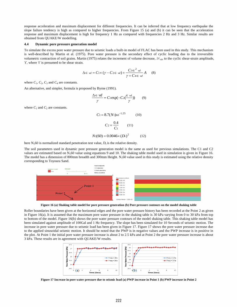
The soil parameters used in dynamic pore pressure generation model is the same as used for previous simulations. The C1 and C2

values are estimated based on N160 value using equations 9 and 10. The shaking table model used in simulation is given in Figure 16.

The model has a dimension of 800mm breadth and 300mm Height. N160 value used in this study is estimated using the relative density corresponding to Toyoura Sand.

Figure 16 (a) Shaking table model for pore pressure generation (b) Pore pressure contours on the model shaking table

Roller boundaries have been given at the horizontal edges and the pore water pressure history has been recorded at the Point 2 as given

in Figure 16(a). It is assumed that the maximum pore water pressure in the shaking table is 30 kPa varying from 0 to 30 kPa from top

to bottom of the model. Figure 16(b) shows the pore water pressure contours of the model shaking table. This shaking table model has

been simulated against amplitude of 100Gal and 1 Hz frequency. The slope has been simulated for 10 Seconds of seismic motion. The

increase in pore water pressure due to seismic load has been given in Figure 17. Figure 17 shows the pore water pressure increase due

to the applied sinusoidal seismic motion. It should be noted that the PWP is in negative values and the PWP increase is in positive in

the plot. At Point 1 the initial pore water pressure increase is about 2 to 2.5 kPa and at Point 2 the pore water pressure increase is about

3 kPa. These results are in agreement with QUAKE/W results.

Figure 17 Increase in pore water pressure due to seismic load (a) PWP increase in Point 1 (b) PWP increase in Point 2

222

5 Comparison of results obtained from numerical codes GeoStudio and FLAC2D

As per the aim of this paper it will be prudent to compare the results obtained from both the numerical codes. In both software codes

the modelling has been performed in same analytical conditions. Broadly two type of analysis have been done one with the slope

model and the other one with the shaking table model. The summary of the analytical conditions considered and the results obtained is given in Table 2.

Table 2 Summary of modelling considerations and results

GeoStudio FLAC2D

Input acceleration (Gal) Factor of safety X

Displacement (mm) Y

Displacement (mm) X

Displacement (mm) Y

Displacement (mm) 100 1.398 1.6 1.06 1.59 1.05 200 1.21 3.11 2.1 3 2.1 300 1.075 4.67 3.1 4.5 3 400 0.9714 6.05 4.03 6 4 500 0.8677 7.7 5.1 Infinity Infinity

Input Freq (Acc=100Gal)

1 1.398 1.6 1.06 1.59 1.05 2 1.4 0.756 0.5 0.796 0.525 3 1.469 0.5 0.335 0.531 0.35

Table 3 Variation in static safety factor

Code GeoStudio FLAC2D

Method FEM FDM SSR

F.O.S 1.562 1.44

From Table 2 it can be noticed that the effect of increasing accelerations obtained from GeoStudio and FLAC2D codes are similar.

Table 3 shows the safety factor variation in static state between SLOPE/W and FLAC codes. Both the numerical modelling tools are

useful in solving dynamic slope stability problems. Quake/W a component of GeoStudio had been used in this study. On the other

hand Itasca’s FDM code FLAC in two dimensions had been used with dynamic option. To present the merits and demerits of the

software codes based on the limited amount of studies performed is cumbersome. Anyhow to clearly understand the components and

basic capabilities of these software codes a brief interpretation had been made based on the modelling methodology of these software

codes. For static slope stability analysis GeoStudio software is useful in consideration to the built in limit equilibrium models. For

PWP estimation GeoStudio analysis had been defined clearly with cyclic shear test terminologies whereas the PWP model in FLAC

has not been clearly defined and should be used with care. For dynamic slope stability analysis both the codes are useful. GeoStudio is

useful to estimate the dynamic safety factor and the analysis is fast compared to FLAC. Even FLAC code doesn’t provide a dynamic safety factor for slope stability value its dynamic feature is attractive and can be used for any type of seismic stability problems.

5.1 General user interface of GeoStudio and FLAC2D

GeoStudio software tool is user friendly having graphical user interface as the only option for modelling. It has the capability of

coupling components like Sigma/W, Quake/W and Slope/W etc. This study used the coupling phenomena to evaluate the dynamic soil

slope stability. The slope geometry for this study had been drawn using built-in graphics tools of the software. FLAC2D numerical

tool is based on FDM and being widely used for soil and rock modelling. FLAC2D has a built in graphical user interface (GIIC) which

enables the user to control the software. Anyhow in this study all the modelling in FLAC2D had been done using command based programming and built-in programming language (FISH).

5.2 Applicability for static slope stability analysis

SLOPE/W is a well-known software tool widely used for slope stability analysis in static state. It has the capacity of coupling with

other GeoStudio components. The factor of safety of the slope is mainly derived based on the method of slices. The stress levels at the

base of each slice can be obtained by limit equilibrium method as well as FEM method. Sigma/W should be used to derive the stress

state of the slope using FEM. The static factor of safety in this study had been estimated based on FEM derived static stress states. The

theory and methodology had been discussed in section 3. FLAC2D is not commonly used for slope stability analysis as the limit

equilibrium models are not provided by the code. Whereas FLAC2D and other Itasca products have inbuilt shear strength reduction

(SSR) technique which serves as an alternative to traditional limit equilibrium analysis in estimating factor of safety of slopes. The

static factor of safety of soil slope in FLAC is estimated using the built-in SSR technique. Also it should be noted that there is a

difference between the static factor of safety of the slope estimated using FEM method in SLOPE/W and SSR method using FLAC2D.

Many researchers have reported the difference in safety factor between limit equilibrium method and SSR method (Cheng et al 2007).

Previous research by Cala and Flisiak (2001) had shown that the safety factor derived from FLAC SSR is lower than safety factors

from limit equilibrium analysis.

5.3 Applicability for dynamic slope stability analysis

The dynamic slope stability analysis performed in both the codes provides different ways of outputs for interpretation of dynamic

behaviour of soil. QUAKE/W component used in this study is capable of solving equivalent linear, equivalent nonlinear and PWP

problems. In this study equivalent linear and PWP models have been used. One of the attractive features of GeoStudio is that the

dynamic factor of safety for the entire earthquake can be obtained for any type of seismic waveforms. The input acceleration is mainly

horizontal and vertical direction components mostly given in units of g (1g=9.87m/s2). The safety factor on this study has been

obtained using the derived dynamic stress levels at base of each slice in coupled SLOPE/W analysis. The theory and estimation

223

procedures are given in section 3. FLAC has optional dynamic analysis tools which can be used for solving linear and nonlinear

seismic problems. But the application of dynamic slope stability in FLAC is not straightforward and deep care should be made when configuring the damping, boundary conditions and dynamic response etc.

5.4 Applicability of pore water pressure generation model

In this study the pore water pressure generation due to seismic loadings has been simulated in both GeoStudio and FLAC2D. In

GeoStudio the method is simple and same as usual dynamic analysis. Pore water pressure increase and excess PWP can be obtained

using dynamic analysis as explained in section 3.3. In a typical finite element analysis the soil strength variables are automatically

recorded for each node and the data can be retrieved any time after the analysis. Whereas in FLAC2D (FDM) all the history variables

needed for interpreting the model must be pre-configured before the cycling starts. The PWP generation model has been used in this

study. The model estimates the increase in PWP for simpler geometries. For finer mesh and large material model the model becomes

slower. However the exact conditions prevailing in model shaking table test can be simulated using FLAC. Behnam et al 2012 and

Moradi et al 2011 have used FLAC2D to simulate the liquefaction potential of soil.

6 Conclusions

Using numerical modelling tools GeoStudio and FLAC2D the soil slope has been simulated against various seismic motions. It is

observed that the numerical modelling tools are robust to solve seismic slope stability problems both in static and dynamic state. Based

on the limited simulations performed the applicability of numerical tools for dynamic slope stability problems have been explained.

This study is an attempt to simulate the behaviour of soil slope in model shaking table test conditions. Due to availability of limited

data of the shaking table test to be performed the simulations have been performed with assumed soil parameters. So far this study had

shown that the built-in constitutive models of FLAC and GeoStudio can be used to precisely simulate the soil slope behaviour for

anticipated earthquake motions. Further numerical simulation studies are aimed to be performed along with model shaking table tests in order to compare and validate the results of numerical and shaking table simulations.

Acknowledgements

The authors are grateful for funding awarded by the Japan Ministry of Education, Culture, Sports, Science and Technology (MEXT)

7 References

Byrne, P. M. (1991). “A Cyclic Shear-Volume Coupling and Pore-Pressure Model for Sand,” in Proceedings: Second International Conference on Recent Advances in Geotechnical Earthquake Engineering and Soil Dynamics (St. Louis, Missouri, March 1991), Paper No. 1.24, 47-55.

Cala M. Flisiak J. (2001). “Slope stability analysis with FLAC and limit equilibrium methods”. In Bilaux, Rachez, Detournay & Hart (eds.) FLAC and Numerical Modelling in Geomechanics: 111-114. A.A. Balkema Publishers

Dawson EM, Roth WH. (1999) “Slope stability analysis with FLAC”, In: FLAC and numerical modelling in Geomechanics. In: Proceedings of the international FLAC symposium on numerical modelling in Geomechanics, Minneapolis, Minnesota; September 1999. p. 3-9.

“Fast Lagrangian Analysis of Continua in 2Dimensions FLAC 2D Manual - FLAC 2D (2006)” Itasca Consulting Group, Minneapolis, U.S.A

GeoStudio - GEOSLOPE International, 2012, Canada

Gholam Moradi, Behnam Rahro Khatibi, Mehdi Hosseinzade Sutubadi (2011). “Determination of Liquefaction Potential of Soil Using (N1)60 by Numerical Modeling Method”. EJGE. Vol. 16, Bund. D.

Kawamura S. and Miura S (2013). “Rainfall-induced failures of volcanic slopes subjected to freezing and thawing”, Soils and Foundations, 53 (30).

Krahn John (2004) “Stability modelling with SLOPE/W - An Engineering Methodology”. GEO-SLOPE/W International Ltd., Alberta, Canada

Krahn John (2004) “Dynamic modelling with QUAKE/W - An Engineering Methodology”. GEO-SLOPE/W International Ltd., Alberta, Canada

Kramer S L (1995) Geotechnical Earthquake Engineering, Prentice Hall, Upper Saddle River, New Jersey

Martin G. R, W. D. L. Finn and H. B. Seed (1975). “Fundamentals of Liquefaction under Cyclic Loading”. J. Geotech., Div. ASCE, 101(GT5), 423-438.

Miura S, Yagi K. (2003). “Mechanical behaviour and particle crushing of volcanic coarse grained soils in Japan”. Characterisation and Engineering Properties of Natural Soils. Tan et al (Eds). Swets and Zeitlinger. Lisse ISBN 90 5809 537 1.

Ozaki Yuta (2004), “Influence of specimen size on strength characteristics of granular materials”. Bachelor thesis, Faculty of Engineering, Hokkaido University.

Seed, H.B, Mori, K, and Chan, C.K, (1975). “Influence of seismic history on the liquefaction characteristics of sands”, Report EERC

75-25, Earthquake Engineering Research Center, University of California, Berkeley, 21pp.

Terzaghi K (1950) “Mechanisms of landslides”. Engineering Geology (Berkey) Volume, Geological Society of America

Y.M. Cheng, T. Lansivaara, W.B. Wei. (2007) “Two-dimensional slope stability analysis by limit equilibrium and strength reduction methods”, Computers and Geotechnics, Volume 34, Issue 3, May 2007, Pages 137-150, ISSN 0266-352X,

Behnam Rahrou Khatibi, Mehdi Hosseinzadeh Sutubadi, Gholam Moradi (2012). “Liquefaction Potential Variations Influenced by Building Constructions”. Earth Science Research; Vol. 1, No. 2; 2012 ISSN 1927-0542 E-ISSN 1927-0550 Published by Canadian Center of Science and Education.

Nabili S, Jafarian Y, Baziar M.H.(2008) “Seismic pore water pressure generation models numerical evaluation and comparison”. The 14th World Conference on Earthquake Engineering. October 12-17, Beijing, China.

224