evaluation of atmospheric pressure loading effects on gps

Evaluation of Atmospheric Pressure Loading

Effects on GPS

H

Examiner: Hans-

Technology

Supervisors: Frank H. Webb, Jet Propulsion Laboratory

Jan M. Johansson, Chalmers

Department of

CHALMERS UNIVERSITY OF TECHNOLOGY

Göteborg, Sweden 2010


Effects on GPS-based Positioning

HERMAN ANDERSSON

-Georg Scherneck, Chalmers University of

Technology

Frank H. Webb, Jet Propulsion Laboratory

Jan M. Johansson, Chalmers University of Technology

Department of Earth and Space Science

CHALMERS UNIVERSITY OF TECHNOLOGY

Göteborg, Sweden 2010


University of Technology

Evaluation of Atmospheric Pressure Loading Effects on GPS-based Positioning

HERMAN ANDERSSON, 2010

Department of Radio and Space Science

Chalmers University of Technology

SE-412 96 Göteborg

Sweden

Cover:

Differences in displacement time series at Bishkek (POL2) with and without

applying the model for atmospheric pressure loading

Chalmers University of Technology

Göteborg, Sweden

ABSTRACT

As atmospheric pressure varies over time it exerts a dynamic load on the

Earth, causing crustal deformations. When performing high precision GPS

measurements, such deformations may affect the accuracy of the

measurements. This Master of Science thesis aims at describing how

atmospheric pressure loading tends to affect precise point positioning with

GPS measurements and evaluate the effects. Furthermore, the goal of the long-

term work, of which this evaluation is part, is to implement correction terms

for crustal movements derived from atmospheric pressure loading in the GPS

data processing software package GIPSY-OASIS and to perform tests to

investigate the results on precise positioning.

Deformation time-series data, based on 6-hourly NCEP reanalysis pressure

data in a 2.5° x 2.5° grid, is downloaded from a database administrated by the

VLBI group at NASA Goddard Space Flight Center. Subsequently, the

deformation data is applied on GPS measurement data as daily average values

and the results are analyzed.

Results from comparing GPS displacement time series data with and without

having applied the model for atmospheric pressure loading, respectively, show

a reduced daily scatter at most of the investigated sites, especially for the

radial component, after implementation of the model. This suggests that

implementing terms of atmospheric pressure loading can enhance the

accuracy in GPS measurements.

Keywords:

Atmospheric pressure loading, crustal deformation, Global Positioning System

(GPS), GPS-Inferred Positioning System – Orbit Analysis Simulation Software

(GIPSY-OASIS), GPS site, time-series, pressure grid

ACKNOWLEDGEMENTS

This Master of Science thesis project has been made possible with help and

support from many people, at Jet Propulsion Laboratory in Pasadena,

California as well as at Chalmers University of Technology in Göteborg,

Sweden, and also my family.

I would especially like to express my gratitude to the following people:

Hans-Georg Scherneck, my examiner at Chalmers University of Technology,

for preparing me for my visit to JPL and sharing his wisdom in the field of

atmospheric loading.

Jan Johansson, my supervisor at Chalmers University of Technology, for

giving me the opportunity to go to JPL, preparing me for my visit and always

being helpful, both with issues directly concerning the project and of more

general nature.

Frank Webb, my supervisor at JPL, for giving me the opportunity to come to

JPL and providing important guidance throughout the project.

Shailen Desai, for giving me supportive guidance and important input to my

work during my visit at JPL.

Angelyn “Angie” Moore, for always being there to answer my numerous

questions concerning everything included in the project and showing patience

with my limitations in programming skills.

Allyson Beatrice, for helping me prepare everything for my visit to JPL and

taking care of everything not directly associated with my project while in

Pasadena so I could focus entirely on my work.

Rob DeCarvalho, my officemate at JPL, for helping me solving all kinds of

problems, big and small, that I encountered in my work, and for all the

interesting discussions during lunches.

Last but not least I would like to thank my wonderful girlfriend Elin for joining

me in California and planning the weekends for us to explore “the Golden

State”, and for always being a great support.

TABLE OF CONTENTS 1. Introduction .......................................................................................................................................... 1

2. Background ........................................................................................................................................... 3

2.1. Global Positioning System ....................................................................................................... 3

2.1.1. Space segment ........................................................................................................................... 4

2.1.2. Control segment ........................................................................................................................ 4

2.1.3. User/receiver segment .......................................................................................................... 5

2.2. GIPSY-OASIS ................................................................................................................................... 6

2.2.1. Software overview ................................................................................................................... 7

2.2.2. gd2p.pl ........................................................................................................................................... 9

2.2.3. GPS Network Processor ..................................................................................................... 10

2.3. NOAA/NCEP Atmospheric Pressure Data ..................................................................... 11

2.4. Inverted Barometer Effect .................................................................................................... 11

3. Implementation ................................................................................................................................ 13

3.1. Acquisition of GPS Time Series Data ................................................................................ 13

3.2. Acquisition of Atmospheric Pressure Loading Data ................................................ 13

3.3. Applying Atmospheric Pressure Loading to Time Series Data ........................... 17

4. Model Verification ........................................................................................................................... 18

4.1. Site selection ................................................................................................................................ 18

4.2. Repeatability analysis ............................................................................................................. 21

4.3. Scatter analysis .......................................................................................................................... 21

4.4. Spectral analysis ........................................................................................................................ 22

5. Results .................................................................................................................................................. 24

5.1. Atmospheric Pressure Loading effects ........................................................................... 24

5.2. Scatter analysis .......................................................................................................................... 30

5.2.1. Standard Deviation ............................................................................................................... 30

5.2.2. Variance ..................................................................................................................................... 32

5.2.3. Possible correlations ........................................................................................................... 34

5.3. Spectral analysis ........................................................................................................................ 36

6. Discussion ........................................................................................................................................... 42

7. Conclusions ........................................................................................................................................ 44

8. References .......................................................................................................................................... 46

APPENDIX

APPENDIX A – GIPSY-OASIS FLOWCHART, SHOWING THE MAIN PROGRAMS AND FILES

APPENDIX B – GREEN’S FUNCTIONS FOR COMPUTING DISPLACEMENTS

1

1. INTRODUCTION In everyday life people are likely to encounter Global Navigation Satellite

Systems (GNSS) such as the American Global Positioning System (GPS), which

has numerous widespread applications. Geophysics, weather forecasting,

navigation and construction are just a few of the fields in which GPS technique

is used. In 1973 the U.S. Department of Defense started developing GPS and

since then there is an ongoing process to improve the system (U.S. National

Executive Committee for Space-Based Positioning, Navigation and Timing,

2009).

As the use of GPS is increasing, so is the demand of the system’s precision and

accuracy. Over the last decade the progress of decreasing error sources

affecting the system has taken a large step forward with advances in receiver

hardware and data analysis software. However, the system is not yet perfect.

One of the remaining error sources in GPS is associated with crustal

movements of the Earth due to atmospheric pressure loading.

The atmosphere exerts a pressure on the Earth’s crust causing elastic

deformation of the solid Earth and thus movements on the ground surface.

The effects of this dynamic load, notably referred to as atmospheric pressure

loading, tend to vary with time as the atmospheric mass distribution changes

globally. The magnitude of the effects fluctuates with time as the pressure

varies, but also depending on location. Oceans tend to reduce the effects of the

atmospheric pressure since large amounts of water can relocate and thereby

absorb the loading. However, the effect is still present in shallow waters. The

amplitude of the caused displacements has proven to be as large as 2 cm in

the vertical direction and 3 mm horizontally (Petrov & Boy, 2004), or comprise

up to 24 % of the total variance in vertical component estimates (van Dam,

Blewitt, & Heflin, 1994) and is thus of importance when computing satellite

orbit data. The Global Positioning System (GPS), which is based on such data,

can be refined by implementing correction terms for ground surface move-

ments derived from atmospheric pressure loading in GPS data processing

software such as GIPSY-OASIS, a software package developed by the National

Aeronautics and Space Administration (NASA) at Jet Propulsion Laboratory

(JPL) in Pasadena, California.

This Master of Science thesis aims at describing influences from atmospheric

pressure loading in connection to GPS measurement data and how

atmospheric pressure loading can affect such measurements. Moreover, the

project is part of an on-going work on implementing correction terms for

atmospheric pressure loading in GIPSY-OASIS. The model is to comprise

meteorological data collected at weather forecasting centers such as the

National Centers for Environmental Prediction (NCEP).

3

2. BACKGROUND This chapter contains descriptions of techniques and technologies essential

for carrying out this project. A summary of how the Global Positioning System

(GPS) works is included, as is a description of the GIPSY-OASIS software as

well as an overview of the meteorological data used.

2.1. GLOBAL POSITIONING SYSTEM The Global Positioning System, GPS, was initially an American military system

for navigational purposes. Originally denoted NAVSTAR (Navigation Satellite

Time And Ranging) GPS has been under development ever since the start in

1973 at the United States Department of Defense (Wells, et al., 1986). Today

the system, which is still owned by the U.S. government, provides various

positioning, navigation and timing (PNT) services not only for military

purposes but also for civilians to use globally. As displayed in Figure 1 below,

GPS is based on interaction between three different segments, namely the

space segment, the control segment and the user/receiver segment (U.S.

National Executive Committee for Space-Based Positioning, Navigation and

Timing, 2009). Below, these three segments and their principles are

described.

FIGURE 1. GPS IS BASED ON INTERACTION BETWEEN THREE DIFFERENT SEGMENTS

2.1.1. SPACE SEGMENT

The space segment consists of 32 (originally 24) satellites orbiting in six

nearly circular orbit planes, inclined 55°. The satellites, operating at a nominal

altitude of 20,180 km with a period of 11 hours and 58 minutes, carry atomic

clocks and continuously transmit unique messages with information about

their position and state, including orbit data and clock parameters. Moreover,

signals are broadcast via two L-band carrier frequencies; L1 (1575.42 MHz)

and L2 (1227.60 MHz) respectively. The L1 carrier is modulated by a military

precision “P-code” at 10.23 MHz along with a civilian course acquisition “C/A-

code” whilst the L2 carrier is modulated only by the P-code. (Wells, et al.,

1986)

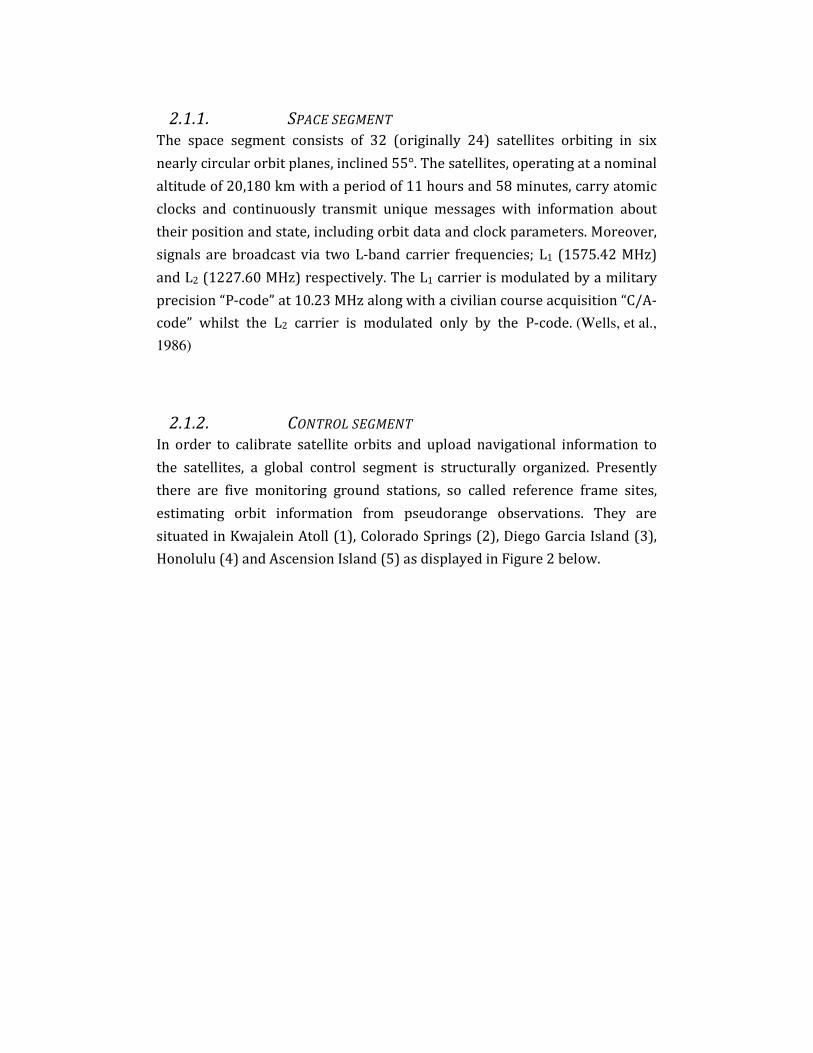
2.1.2. CONTROL SEGMENT

In order to calibrate satellite orbits and upload navigational information to

the satellites, a global control segment is structurally organized. Presently

there are five monitoring ground stations, so called reference frame sites,

estimating orbit information from pseudorange observations. They are

situated in Kwajalein Atoll (1), Colorado Springs (2), Diego Garcia Island (3),

Honolulu (4) and Ascension Island (5) as displayed in Figure 2 below.

5

FIGURE 2. THE IGS TRACKING NETWORK WITH REFERENCE FRAME SITES HIGHLIGHTED IN

RED

The five reference frame sites belong to the IGS (International GNSS Service)

tracking network consisting of numerous GPS stations spread all over the

world, tracking both code and phase data from at least eight visible satellites

simultaneously. Such stations can be operated and controlled by practically

anyone who can meet the requirements of the IGS Site Guidelines established

at the IGS Central Bureau (IGS Central Bureau, 2007). The IGS Site Guidelines

include requirements on submitting tracking data, meteorological data and

timing activities amongst others. For each included field there are some

equipment and operational characteristics that are “strictly required” and

some that are “additionally desired”, meaning that the features of the different

stations in the IGS tracking network vary, which may need to be taken into

consideration when using the tracking stations for analysis.

2.1.3. USER/RECEIVER SEGMENT

The third segment needed in GPS measurement is the user/receiver segment.

This is where the signals sent out from the satellites in the space segment are

acquired and interpreted. The basic idea behind this step is to measure the

difference between the time a message is sent from a satellite and the time it

is collected by a receiver, and then calculate the distance according to

equation 1 below. The distance between a satellite and a receiver is usually

denoted pseudorange.

� = � ∙ (�� − ��) (1) where,

R is the pseudorange,

c is the speed of light,

tr is the time when the signal reaches the receiver and

tsat is the time when the signal is sent from the satellite.

As modern receivers have parallel working channels, it is possible to acquire

several satellites simultaneously. As mentioned earlier, all satellites transmit

unique code sequences and thus the receivers are able to separate the

different satellites from one another. Accordingly, receivers can determine

their position from knowledge of the distances to multiple satellites.

There is, however, a more precise alternative to this traditional method of

code based positioning using the carrier phase instead. By measuring the

phase difference between the generated and the received code, millimeter

precision can be obtained. This more precise method is used in this project.

Regardless of which method is used, receivers commonly consist of three

main components; an antenna, a receiver-processor unit and a

control/display.

In general, the accuracy of GPS positioning depends on the geometric

constellation of the satellites used and the precision of a single pseudorange is

commonly expressed by the standard deviation, σr. When describing the

associated error in position, the term Dilution Of Precision, DOP, is

introduced. As the accuracy is depending on satellite orbit constellation the

DOP is not the same in all directions, north, east and vertical, and applies also

on time measurements. (Seeber, 1993)

2.2. GIPSY-OASIS GPS data can be collected and processed by using the software package GIPSY-

OASIS, which consists of two parts with common modules. The first part,

GIPSY, short for GPS-Inferred Positioning System, is intended for standard

geodetic applications while the second part, OASIS (Orbit Analysis Simulation

Software), is a software package for analysis of orbit data covariance. JPL

started developing the software in 1985 and it has developed and improved

ever since. The current version of G

system and can be used for pro

(Satellite Laser Ranging), TOPEX

(Doppler Orbitography and Radio posi

observations. (Gregorius, 1996)

2.2.1. SOFTWARE OVERVIEW

A flowchart thoroughly displaying the outline of the

software is enclosed in appendix

components of the software package and the

namely obervational data and orbit data.

an overview of what steps are in

FIGURE 3. A TYPICAL GIPSY

7

Inferred Positioning System, is intended for standard

cations while the second part, OASIS (Orbit Analysis Simulation



ever since. The current version of GIPSY-OASIS runs on the UNIX operating

system and can be used for processing not only GPS data but also SLR

(Satellite Laser Ranging), TOPEX (TOPography Experiment) and DORIS

(Doppler Orbitography and Radio positioning Integrated by Satellite)

(Gregorius, 1996)

OFTWARE OVERVIEW

displaying the outline of the traditional GIPSY

ware is enclosed in appendix A. The flowchart shows the main

components of the software package and the two main input branches,

namely obervational data and orbit data. The chart in Figure 3 below shows

an overview of what steps are included in a typical GIPSY-OASIS data flow.

A TYPICAL GIPSY-OASIS DATA FLOW (JET PROPULSION LABORATORY, 2010)

Inferred Positioning System, is intended for standard

cations while the second part, OASIS (Orbit Analysis Simulation



OASIS runs on the UNIX operating

cessing not only GPS data but also SLR

and DORIS

grated by Satellite)

GIPSY-OASIS

. The flowchart shows the main

two main input branches,

below shows

OASIS data flow.

RATORY, 2010)

Data consisting of satellite observations is collected in a RINEX file, which is

the input to a program file called ninja. RINEX (Reciever Independent

Exchange) files are, as the name suggests, independent of what receiver they

are collected from. There are two kinds of RINEX files, namely single

frequency and double frequency. Single frequency files hold only carrier wave

data from L1 and code data from C1, while double frequency RINEX files

consist of carrier wave data from both L1 and L2 as well as code data from

both C1 and C2 (Gutner, 2002). The ninja program reads the RINEX files,

reorders the data and writes the satellite data to individual binary fortran

files, called quick measurement, qm, files. The individual qm files are then

merged into a single file with the help of a program called merg_qm. Two

scripts, qr_nml and s2nml, are used for creating a so called qregres namelist,

suitable for the subsequent qregres program, from a merged qm file and other

station information.

The other input data branch, containing satellite orbit data, begins with an

orbit generator script called genoi. This script works with two namelists,

tp.nml containing data of time along with polar motion and trajedy.nml

containing satellite orbit data. The orbit generator module creates so called oi

files consisting of satellite state data including position, velocity, acceleration

and partials as a function of time. In the same way as several qm files were

merged into one with the use of merg_qm, merge_sat is used in order to merge

several oi files into one that can be added to the qregres namelist mentioned

above. (Gregorius, 1996)

The qregres namelist is put into the qregres program, which interprets the

namelist values and applies built-in physical models in order to create a

regres file called rgfile, adjusted according to the models. The physical models

hold correction terms concerned with measurement and Earth models,

including tidal effects, phase centre offset, clock behavior and tropospheric

effects, among many other (Gregorius, 1996). The output regres file is

prepared for the following filtering process, starting with two steps of basic

preparation for the actual filtering algorithm coming into play in a module

simply called filter. The filtering algorithm is a modified Kalman filter called

9

Square Root Information Filter (SRIF), producing up to five optional output

files with the final arrays along with smoothing coefficients, transition

matrices and other parameters.

Subsequently, a function called smapper computes and maps the covariance,

sensitivity and solution before post-fit data residuals are calculated by the

postfit script. The output file, postfit.nio, carries both the pre- and post-fitted

residuals. The postbreak command is then used for discovering

discontinuities in the postfit.nio file. If previously passed on cycle slips are

present the procedure is re-run with a modified qm file. If no cycle slips are

found, however, outliers in the filtered output data are deleted with edtpnt2.

After that step the smapper and postfit functions have to be re-run with the

updated data files. The user can then evaluate the results and verify that no

points need to be rejected. If modifications are needed the results are looped

back to edtpnt2 for readjustment. If the results seem satisfying, however, they

are passed on to the stacov software tools, which are used for creating

readable text files. The ambigon2 script is an optional tool for adjusting the

ambiguity resolution in order to obtain a more bias-free outcome. (Gregorius,

1996)

The stacov software tools, including the programs stacov, heightfix, stamrg,

project, statistics and transform, interpret the smcov.nio file and, as

previously mentioned, create readable output files. The output data is stored

in so called stacov files, in ASCII format, to be interpreted and used directly or

for further post-processing. (Gregorius, 1996)

2.2.2. GD2P.PL

As mentioned earlier, the GIPSY-OASIS software is under continuous

development. An important step in the progress came in late 2008 with the

new program gd2p.pl, short for GPS Data to Position. The program, written in

the programming language Perl, works as a part of the traditional GIPSY-

OASIS software and uses many of the already featured modules but, however,

takes over the roles of others. gd2p.pl can be used for static and kinematic

point positioning as well as precise orbit determination.

The outcome of running gd2p.pl is not only the final position solution, named

tdp_final, but also three other important files. An executable script called

run_again is created for running the program again, allowing the user to

either keep the options used previously or make modifications. In addition,

eventual errors are collected in gd2p.err while gd2p.log can provide a log of

which GIPSY programs where executed and how. (Jet Propulsion Laboratory,

2008)

2.2.3. GPS NETWORK PROCESSOR

Over the past years new software has been developed at JPL for efficient

processing of GPS ground station data from large networks. The software,

called GPS Network Processor, runs with modules from GIPSY-OASIS using

precise point positioning and bias fixing. In conformity with regular use of

GIPSY-OASIS, the network processor has a command line interface where the

user can decide what software features to use or not to use.

The GPS Network Processor software consists of three main programs, simply

called a.pl, b.pl and c.pl. At start, the software expects a RINEX archive with

station data at the local computer where the processing is to take place, from

where files are copied to a directory called pp_input. The first main program,

a.pl, moves input RINEX files from pp_input to another directory called

pp_in_process, and initializes the script run_gd2p.pl, which point positions the

RINEX files and places the results in a tree under the pp_output directory

organized by year and day. The second program, b.pl, runs the script

run_amb_day.pl for each day, either creating clusters of sites or keeping the

sites separate, if desired, and then performing ambiguity resolution on each

baseline. The results, ending up in a year and day of year tree under a

directory called amb_output are then merged into one single stacov file in a

directory called mrg_final for the user to view. The third program, c.pl, finally

runs the script run_staproject.pl for each day. The script transforms the stacov

file containing the final result to International Terrestrial Reference System

(ITRF) coordinates and gets rid of the included covariance matrix. At last, the

ultimate results are copied to an archive directory specified by the user.

(Newport, 2006)

11

2.3. NOAA/NCEP ATMOSPHERIC PRESSURE DATA National Centers for Environmental Prediction (NCEP) is part of the U.S.

National Weather Service (NWS), which in its turn is governed by the National

Oceanic and Atmospheric Administration (NOAA). NCEP provides national as

well as international meteorological data and statistics used in many

instances; governmental, corporative and private. (NOAA, 2007)

Global pressure field reanalysis data for the atmospheric loading data used in

this project is provided by NCEP at the Computational and Information

Systems Laboratory (CISL) Research Data Archive in 6-hourly data sets,

collected each day at 0:00 UT, 6:00 UT, 12:00 UT and 18:00 UT, in a 2.5° x 2.5°

grid.

2.4. INVERTED BAROMETER EFFECT At sea the concept of an Inverted Barometer Effect, IBE, is often used for

estimating elastic fluctuations of the sea level due to atmospheric loading.

Moreover, IBE is not only present at sea but also comes into play over land.

The effects, however, are not as large as they are at sea. By IBE is understood

both vertical and horizontal movements of mass in connection to atmospheric

pressure loading at ground surface. It bases on the trivial principles of

pressure behavior, saying that elastic bodies deform and move their mass

towards low-pressure environments. (Wunsch & Stammer, 1997)

The magnitude of the effect is most often expressed by the direction

dependant ratios between the crustal response and the exerted atmospheric

pressure. In the vertical direction the ratio is approximately 0.4 mm/hPa on

land (approximately 10 mm/hPa at sea), but the figure is highly dependent on

the properties of the underlying soil. Thus, sites located in the vicinity of a

coastline or on an island will respond differently than inland sites to an equal

magnitude of atmospheric pressure loading (van Dam, Blewitt, & Heflin, 1994).

The sketch in Figure 4 below shows a two dimensional example of the

Inverted Barometer Effect, IBE.

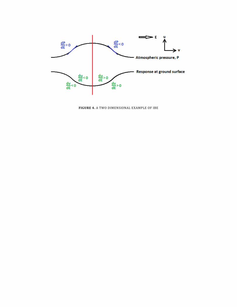
FIGURE 4. A TWO DIMENSIONAL EXAMPLE OF IBE

13

3. IMPLEMENTATION The implementation part of this project can be divided into two different

development processes. The first part comprises software development for

collecting atmospheric pressure loading data in grids with appropriate

resolution. The second part consists of developing new GIPSY interfaces for

comprehensive modeling of east, north and vertical movements caused by

atmospheric pressure loading. Moreover, the both parts need to be

compatible with one another, thus contain data sets with agreeing units,

formats and coordinate systems.

3.1. ACQUISITION OF GPS TIME SERIES DATA The analysis is based on GPS tracking data collected using GIPSY-OASIS

software, as previously described. Initially, GPS position data is processed for

a period of time from May 1st 2009 through June 29th 2010 for a number of

chosen stations with the GPS Network Processor. Subsequently a program

called staseries is used for creating time series from the individual location

data. The program staseries is, as most other GIPSY-related programs, based

on a command line user interface, where a file containing the reference

location of a certain station is declared followed by the other files to be

combined in the time series and optional user preferences. Time series have

to be created for each station individually using staseries.

Running staseries gives output in the form of three files for each station; one

with latitude (*.lat), one with longitude (*.lon) and one containing radial

component data (*.rad). An optional feature, which is used in this project, is to

also include position residuals in the staseries results.

3.2. ACQUISITION OF ATMOSPHERIC PRESSURE LOADING DATA For the implementation of atmospheric pressure loading in the analysis,

atmospheric pressure loading time series are provided by the Goddard Very

Long Baseline Interferometry (VLBI) group at NASA Goddard Space Flight

Center; available on the Web at http://gemini.gsfc.nasa.gov/aplo (Petrov &

Boy, 2004). Below is described in short the method used for calculating

atmospheric loading from atmospheric pressure data.

Reanalysis pressure data is, as previously mentioned, collected from NCEP at

CISL Research Data Archive in 6-hourly data sets over a 2.5° x 2.5° grid.

Moreover, the original data files contain ground or sea level pressure data,

expressed in Pascal (Pa) along with longitude, latitude and geopotential

height for each point in the grid. The model gives mean surface pressure and

comprises a model of diurnal and semi-diurnal variations computed from

NCEP reanalysis data over a period of time spanning from 1980 through 2002.

(Petrov, Atmospheric Pressure Loading Service, 2008)

Using the pressure data, global distribution of atmospheric pressure loading

is computed by Green’s functions, presented in appendix B, in accordance

with Farrell (1972) and bases on the Preliminary Reference Earth Model

(PREM). PREM is an extensive data set containing a radial model of the Earth

with numerous geophysical parameters, such as distribution of density and

seismic velocities (Dziewonski & Anderson, 1981). The displacements derived

from atmospheric pressure loading are calculated in relation to the center of

mass of the solid Earth and the atmosphere combined. (Petrov, Atmospheric

Pressure Loading Service, 2008)

In order to obtain an accurate and sufficiently precise model of the oceanic

boundaries, the FES99 land-sea mask with 0.25° x 0.25° resolution was used.

The oceanic response to atmospheric loading was then computed in

accordance with the previously described inverted barometer effect theory

(Petrov, Atmospheric Pressure Loading Service, 2008). The plots in Figure 5

show amplitudes of the displacements caused by the diurnal (S1) and semi-

diurnal (S2) variations in atmospheric loading according to the model.

FIGURE 5. DISPLACEMENT CAUSED

IN ATMOSPHERIC PRESSURE

As van Dam, Altamimi, Collilieux and Ray

resolution of the reanalysis pressure data grid

concern due to considerable topographic variation within grid cells. Since a

large variation in topography typica

pressure, it may seem relevant to use a somewhat finer grid in mountainous

regions. However, van Dam, Altami

incentives for settling with the coarse grid. Firstly, their study indicates that

less than 4 % of the grid points in the NCEP

15

DISPLACEMENT CAUSED BY DIURNAL (S1) AND SEMI-DIURNAL (S2) VARIATIONS

URE (PETROV, ATMOSPHERIC PRESSURE LOADING SER

2008)

i, Collilieux and Ray (2009) suggest, the rather coarse

lution of the reanalysis pressure data grid (2.5° x 2.5°) may be a cause for


large variation in topography typically gives large differences in atmospheric


van Dam, Altamimi, Collilieux and Ray (2009) present two


the grid points in the NCEP 2.5° x 2.5° grid show variations

) VARIATIONS

PRESSURE LOADING SERVICE,

suggest, the rather coarse

may be a cause for


lly gives large differences in atmospheric


present two


show variations

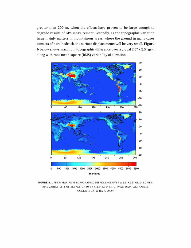
greater than 200 m, when the effects have proven to be large enough to

degrade results of GPS measurement

issue mainly matters in mountainous areas, where the ground in many cases

consists of hard bedrock, the surface displacements will be very small.

6 below shows maximum topographic difference over a global

along with root-mean-square

FIGURE 6. UPPER: MAXIMUM TOPOGRAPHIC

RMS VARIABILITY OF ELEVA

, when the effects have proven to be large enough to

lts of GPS measurement. Secondly, as the topographic variation


consists of hard bedrock, the surface displacements will be very small.

shows maximum topographic difference over a global 2.5° x 2.5

square (RMS) variability of elevation.

MAXIMUM TOPOGRAPHIC DIFFERENCE OVER A 2.5°X2.5° GRID. LOWER:

VARIABILITY OF ELEVATION OVER A 2.5°X2.5° GRID. (VAN DAM, ALTAMIMI,

COLLILIEUX, & RAY, 2009)

, when the effects have proven to be large enough to

graphic variation


consists of hard bedrock, the surface displacements will be very small. Figure

x 2.5° grid

GRID. LOWER:

(VAN DAM, ALTAMIMI,

17

3.3. APPLYING ATMOSPHERIC PRESSURE LOADING TO TIME

SERIES DATA When finally combining the two preceding steps, the displacement vectors

caused by atmospheric pressure loading is subtracted from the original time

series data, according to the principle commonly referred to as o – c (or omc),

meaning observed data minus computed data. This principle is generally used

in GPS processing when correcting observational data.

For this particular project, a program was written in Perl programming

language to read observed and computed data in order to subtract the

displacements caused by the atmospheric pressure loading. The program

outputs time series data in the same format as the original, non-corrected,

time series data in order to facilitate use of the corrected data and comparison

between the two. Before applying the model on the time series data, daily

averages where created from the provided 6-hourly atmospheric pressure

loading data, in order to decrease the influence from diurnal and semi-diurnal

variation.

4. MODEL VERIFICATION Throughout the implementation process GPS site data has been used for

testing processing software and analyzing the results. Below is described the

approach for testing and verifying the accuracy of the implementation model.

4.1. SITE SELECTION All stations used in the project belong to the IGS tracking network and are

considered to provide consistent and reliable data for the analysis. Apart from

this, the choice of stations is also based on location. In order to obtain a broad

variety of data with all types of variations in atmospheric loading the selected

sites are spread globally.

For the analysis, all used stations are also situated at least 500 km from the nearest

ocean coastline in order to avoid interference from ocean loading and tidal effects. The

total number of stations used is 29, which is considered to be large enough to provide

reliable results but still small enough for the processing to be performed within a

reasonable amount of time. Below, Figure 7 displays a map showing the locations of all

sites used in the analysis whilst a complete list of the stations is shown in

Table 1.

FIGURE 7. THE COLORED DOTS REP

COLORS INDICATE DISTANCE TO NEAREST OCEA

BOTTOM. NOTE THAT ALL

19

THE COLORED DOTS REPRESENT THE 29 STATIONS USED IN THE ANALY

ANCE TO NEAREST OCEAN ACCORDING TO THE SCALE AT THE

. NOTE THAT ALL STATIONS ARE SITUATED AT LEAST 500 KM FROM

NEAREST OCEAN SHORE.

NS USED IN THE ANALYSIS. THE

AT THE

THE

TABLE 1. THE 29 STATIONS USED IN THE ANALYSIS

Station

ID No. Location Country Lon (E) Lat (N)

Altitude

(m)

Dist. to

coast (m)

ALGO 1 Algonquin Park Canada 281,9286 45,9588 201,4 538431

ALIC 2 Alice Springs Australia 133,8855 -23,6701 603,7 899809

AMC2 3 Colorado Springs U.S.A. 255,4754 38,8031 1912,5 1149910

BRAZ 4 Brasilia Brazil 312,1222 -15,9474 1106,0 860715

CHUM 5 Chumysh Kazakhstan 74,7511 42,9985 716,3 2077430

DUBO 6 Lac Du Bonnet Canada 264,1338 50,2588 251,0 773545

FLIN 7 CFS Flin Flon Canada 258,0220 54,7256 320,0 627010

IRKJ 8 Irkutsk Russia 104,3162 52,2190 502,1 1785250

KIT3 9 Kitab Uzbekistan 66,8800 39,1400 643,0 1505810

KUNM 10 Kunming China 102,7972 25,0295 1986,2 607385

LHAZ 11 Lhasa China 91,1040 29,6573 3622,0 766567

MBAR 12 Mbarara Uganda 30,7379 -0,6015 1337,7 1047310

MDO1 13 Fort Davis U.S.A. 255,9850 30,6805 2004,5 689398

MDVJ 14 Mendeleevo Russia 37,2145 56,0215 257,4 596298

NLIB 15 North Liberty U.S.A. 268,4251 41,7716 207,1 1266130

NVSK 16 Novosibirsk Russia 83,2355 54,8406 123,6 1399710

PICL 17 Pickle Lake Canada 269,8380 51,4798 315,1 533360

PIE1 18 Pie Town U.S.A. 251,8811 34,3015 2347,7 579328

POL2 19 Bishkek Kyrgyzstan 74,6943 42,6798 1714,2 2043210

PRDS 20 Calgary Canada 245,7065 50,8713 1247,0 632610

SELE 21 Almaty Kazakhstan 77,0168 43,1791 1340,0 2178380

SULP 22 Lviv Ukraine 24,0145 49,8356 370,5 584023

TEHN 23 Tehran Iran 51,3341 35,6973 1194,6 615699

ULAB 24 Ulaanbataar Mongolia 107,0500 47,67 1611,7 1299190

UNSA 25 Salta Argentina 294,5924 -24,7275 1257,8 509277

URUM 26 Urumqi China 87,6300 43,59 856,1 2357430

WUHN 27 Wuhan City China 114,3573 30,5317 25,8 568800

XIAN 28 Lintong China 109,2215 34,3687 81,6 882602

YELL 29 Yellowknife Canada 245,5193 62,4809 181,0 583112

An alternative approach towards avoiding ocean loading intervention could

be to base the choice of stations on the size of the ocean loading coefficients at

each station, i.e. use stations with ocean loading coefficients less than a

certain threshold value. This approach, however, was not used because of the

fact that ocean loading coefficients have daily variation. As in this project daily

average values are used for calculating atmospheric pressure loading, the

daily variation in ocean loading may bring that ocean loading is applicable at

certain stations at some points in time although the coefficients fall below the

threshold in average over the day.

Moreover, no considerations concerning properties of the underlying rock or

soil structures at the stations are taken into account in the project. It is likely

that this affects the loading behavior, but as the pressure grid is rather coarse

21

(2.5° x 2.5°) the variation within each bin area is too great to model

comprehensibly.

4.2. REPEATABILITY ANALYSIS In order to analyze the accuracy of the results, time series are created by

combining stacov files for each individual site, both with and without having

applied correction terms for atmospheric pressure loading. As previously

mentioned, the time series span from May 1st 2009 through June 29th 2010.

The resulting time series, which are created using the program staseries,

include site coordinates, repeatability about the initial reference position and

residuals.

4.3. SCATTER ANALYSIS The quality of the displacement data can be assessed by comparing the daily

scatter within the time series before and after having applied terms of

atmospheric loading. This is done by comparing standard deviation and

variance for each time series. A reduction in scatter, thus reduction of

standard deviation and variance, indicates a superior solution. Before per-

forming the scatter analysis, outliers with values farther from the sample

mean than three times the standard deviation are eliminated from the time

series displacement data.

Prior to the scatter analysis the time series data is also prepared by

subtracting the sample mean and removing eventual obvious trends within

the data sets. Trends are removed by subtracting the equation of a line, fitted

to the curve of the original data, from the displacement time series data. In

order to reduce influence from annual behavior, a sine curve is fitted to each

time series and subsequently subtracted. This procedure gives bias-free time

series data with reduced power from linear and annual trends for the

analysis.

In Figure 8 below, plot A (top left) shows the original time series in red with

the mean value in black. Plot B (top right) shows the same time series after

subtracting the mean in green and a fitted linear regression in black.

(bottom left) shows the time series after subt

blue and a fitted sine curve in black whilst plot D (bottom right) shows the

final time series, prepared for further analysis.

FIGURE 8. AN EXAMPLE OF

ANALYSIS, TAKEN FROM THE STATI

4.4. SPECTRAL ANALYSIS

The periodogram is a tool for investigating periodic tendencies within time

series data spectra. In this project

power and frequency as w

subtracting the mean in green and a fitted linear regression in black.

(bottom left) shows the time series after subtracting the linear regression in

nd a fitted sine curve in black whilst plot D (bottom right) shows the

final time series, prepared for further analysis.

AN EXAMPLE OF THE PROCEDURE OF PREPARING TIME SERIES DATA F

TAKEN FROM THE STATION IN YELLOWKNIFE (YELL)

PECTRAL ANALYSIS The periodogram is a tool for investigating periodic tendencies within time

s data spectra. In this project it is used for finding relations between

as well as amplitude and frequency, respectively,

subtracting the mean in green and a fitted linear regression in black. Plot C

cting the linear regression in

nd a fitted sine curve in black whilst plot D (bottom right) shows the

G TIME SERIES DATA FOR

The periodogram is a tool for investigating periodic tendencies within time

it is used for finding relations between

ell as amplitude and frequency, respectively, among

23

the time series data. As for the scatter analysis, described above, outliers are

eliminated before performing spectral analysis and linear trends are removed

as well as annual tendencies. The program pdgram, written in Perl, then

computes Fourier transformation and smoothes the periodogram results in

order to provide comprehensible output data.

5. RESULTS The results of the model verification, described in the previous chapter, imply

that a higher degree of accuracy can be obtained by implementing

atmospheric pressure loading in high precision GPS measurement. Below, the

results from each step of the model verification process are presented.

5.1. ATMOSPHERIC PRESSURE LOADING EFFECTS According to above, time series are created with and without applying the

model of atmospheric pressure loading effects. Figure 9 shows an example of

time series for Bishkek, Kyrgyzstan in latitudinal, longitudinal and radial

directions, respectively. The red lines represent the case where no

atmospheric pressure loading model is applied and the green lines represent

the case with having applied the model.

FIGURE 9. DISPLACEMENT TIME SE

Comparing the differences in displacement after applying the model for

atmospheric pressure loading to the original time series gives the direct

effects of the model, and thus the loading

example of this, again for Bishkek, is

the model has the most im

this site vary from -1.67 cm to 0.86 cm

displacement of 0.42 cm

period of time in the latitudinal direction and

longitudinally.

25

DISPLACEMENT TIME SERIES FOR BISHKEK (POL2)

the differences in displacement after applying the model for

essure loading to the original time series gives the direct

effects of the model, and thus the loading, assuming the model is correct. An

example of this, again for Bishkek, is shown in Figure 10. The plots show that

the model has the most impact on the vertical component, where estimates at

1.67 cm to 0.86 cm. Atmospheric pressure loading causes

.42 cm at maximum at Bishkek during the investigated

in the latitudinal direction and half as much, 0.21 cm

the differences in displacement after applying the model for

essure loading to the original time series gives the direct

the model is correct. An

The plots show that

, where estimates at

ressure loading causes

during the investigated

0.21 cm,

FIGURE 10. DIFFERENCES IN DISPL

WITHOUT APPLYING THE MODEL FOR

The plots in Figure 11

displacement caused by atmospheric pressure loading

standard deviation (blue bars), indicate that it is not only at Bishkek the

largest impact is seen in the radial direction, but for all other stations in

in the analysis as well. Further

the model in the longitudinal direction whilst the latitude is affected slightly

more. The displacements in the radial direction, however, are significantly

larger. Note that plotted means are absolu

negative) only determine the directions of dis

DIFFERENCES IN DISPLACEMENT TIME SERIES AT BISHKEK (POL2) WITH AND

LYING THE MODEL FOR ATMOSPHERIC PRESSURE LOADING

11, showing averages (red circles) of suggested

displacement caused by atmospheric pressure loading at each station and


largest impact is seen in the radial direction, but for all other stations in

Furthermore, most results show the least impact from

tudinal direction whilst the latitude is affected slightly


Note that plotted means are absolute values and the signs (positive or

negative) only determine the directions of displacement.

WITH AND

LOADING

of suggested

at each station and


largest impact is seen in the radial direction, but for all other stations included

more, most results show the least impact from

tudinal direction whilst the latitude is affected slightly


te values and the signs (positive or

Figure 11. The red circles represent

pressure loading at each station. The blue bars show stan

numbered according to

27

The red circles represent mean displacement caused by Atmospheric

pressure loading at each station. The blue bars show standard deviation. Stations are

mean displacement caused by Atmospheric

dard deviation. Stations are

TABLE 1.

Looking at maximum displacement caused by atmospheric pressure loading it

is, again, obvious that the largest movements are found in the vertical

direction.

Typically, maximum values for longitudinal displacement are less than 5 mm

while they in average are 5 mm for the latitude and 15 mm for the radial,

reaching as high as 32 mm at one point at the station in Novosibirsk, Russia

(NVSK). The maximum displacements due to the modeled atmospheric

pressure loading are shown as red circles in Figure 12 with standard

deviations represented by blue bars. Again, note that maximums are absolute

values and the signs only show the directions of displacement.

Figure 12. The red circles represent maximum displacement caused by Atmospheric


numbered according to

29

The red circles represent maximum displacement caused by Atmospheric


The red circles represent maximum displacement caused by Atmospheric


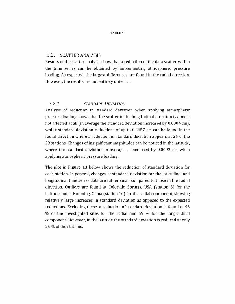
TABLE 1.

5.2. SCATTER ANALYSIS Results of the scatter analysis show that a reduction of the data scatter within

the time series can be obtained by implementing atmospheric pressure

loading. As expected, the largest differences are found in the radial direction.

However, the results are not entirely univocal.

5.2.1. STANDARD DEVIATION

Analysis of reduction in standard deviation when applying atmospheric

pressure loading shows that the scatter in the longitudinal direction is almost

not affected at all (in average the standard deviation increased by 0.0004 cm),

whilst standard deviation reductions of up to 0.2657 cm can be found in the

radial direction where a reduction of standard deviation appears at 26 of the

29 stations. Changes of insignificant magnitudes can be noticed in the latitude,

where the standard deviation in average is increased by 0.0092 cm when

applying atmospheric pressure loading.

The plot in Figure 13 below shows the reduction of standard deviation for

each station. In general, changes of standard deviation for the latitudinal and

longitudinal time series data are rather small compared to those in the radial

direction. Outliers are found at Colorado Springs, USA (station 3) for the

latitude and at Kunming, China (station 10) for the radial component, showing

relatively large increases in standard deviation as opposed to the expected

reductions. Excluding these, a reduction of standard deviation is found at 93

% of the investigated sites for the radial and 59 % for the longitudinal

component. However, in the latitude the standard deviation is reduced at only

25 % of the stations.

Figure 13. Reduction of standard deviation with Station numbers according to

31

Reduction of standard deviation with Station numbers according to

Reduction of standard deviation with Station numbers according to

TABLE 1.

5.2.2. VARIANCE

Since the magnitude of displacement varies significantly between different

stations within the analysis it is important not only to investigate the scatter

reduction in terms of absolute figures, but also as percentual reduction of an

initial value. A convenient way of doing this is by looking at variance.

Figure 14, showing percentual reduction of variance for each of the

investigated sites, reveals that rather large percentual changes in variance are

present in the radial and latitudinal directions while only small changes are

seen in the longitude. At the most, the radial component variance is reduced

by 61 % (in Irkutsk, Russia). Excluding the outlier found in Colorado Springs,

USA, the maximum percentual change in variance for the latitude is an

increase of 28 %, found in Lhasa, China.

In average, variance is reduced by 28 % for the radial direction, while it was

increased by 6 % (if excluding the outlier at the station in Colorado Springs)

for the latitude. The longitude was as good as unaffected.

Figure 14. Percentual reduction of variance with station numbers

33

Percentual reduction of variance with station numbers according to

according to

TABLE 1.

5.2.3. POSSIBLE CORRELATIONS

As described earlier, the magnitude of atmospheric pressure and thus

atmospheric pressure loading is highly dependant on altitude. Accordingly,

the meteorological data must be precise enough to give correct values of

atmospheric pressure and the model for calculating and interpolating the

derived loading to the specific sites must be precise enough to model the

loading distribution correctly.

If the model would fail to describe the loading, trends may appear as results of

correlation between altitude and measured displacement. However, plotting

reduction of standard deviation against the altitudes at which the stations are

located, as displayed in Figure 15, suggests that no such correlation exists at

the sites included in this project.

FIGURE 15. REDUCTION OF STANDAR

In the same way as for altitude,

shoreline may interfere with displacement data. If the model of atmospheric

pressure loading fails to account for differences between oceanic behavior

and the loading response over l

unwanted biases.

The results from plotting reduction of standard deviation against distance to

nearest ocean, as seen in

the plot with standard deviation against altitude. The reason for this is that

the stations included in the analysis are all chosen because they are situated

at a great distance from nearest shoreline.

35

REDUCTION OF STANDARD DEVIATION PLOTTED AGAINST ALTITUDE

the same way as for altitude, effects related to the distance to nearest



and the loading response over land, the results may be affected and thus carry

results from plotting reduction of standard deviation against distance to

nearest ocean, as seen in Figure 16, are however not as easily interpreted as



at a great distance from nearest shoreline. Thus, the plot does not necessarily

AGAINST ALTITUDE

the distance to nearest



and, the results may be affected and thus carry

results from plotting reduction of standard deviation against distance to

, are however not as easily interpreted as



Thus, the plot does not necessarily

suggest that there is no correlation between the results and the distance to

coast, although no signs of such a correlation can be found, but rather that all

stations are situated sufficiently far from the closest ocean

FIGURE 16. REDUCTION OF STANDAR

5.3. SPECTRAL ANALYSIS

Before implementing the atmospheric pressure loading model, time series

data was dominated by an

amounts of noise affected the signal.

found for the semi-annual frequencies in the power spectra.

model, the annual peak is reduced at most stations



stations are situated sufficiently far from the closest ocean to be affected by it.

REDUCTION OF STANDARD DEVIATION PLOTTED AGAINST DISTANCE TO

NEAREST COASTLINE.

PECTRAL ANALYSIS Before implementing the atmospheric pressure loading model, time series

data was dominated by an annual power and as frequency increased, larger

amounts of noise affected the signal. At many sites an additional peak can be

annual frequencies in the power spectra. By applying the

model, the annual peak is reduced at most stations but only small



to be affected by it.

AGAINST DISTANCE TO

Before implementing the atmospheric pressure loading model, time series

annual power and as frequency increased, larger

At many sites an additional peak can be

By applying the

only small

37

improvements can be found in the high frequency noise. The semi-annual

peaks are reduced to some extent, but generally not as much as the annual.

As the statistical scatter analysis above showed, the largest alterations

between before and after applying the model of atmospheric pressure loading

are found in the radial direction. Therefore, the spectral analysis is focused

mainly on vertical displacement data. Periodograms of signals in the

latitudinal and longitudinal directions, however, typically show the same

effect as in the radial only with smaller differences between the two cases;

with and without applied atmospheric pressure loading, respectively.

Figure 17 shows a log-scale periodogram of radial time series data from

Irkutsk, Russia. The red line represents the case where no model of

atmospheric pressure loading is applied, and the green line represents the

case after implementing the model. Power reductions are found at most

frequencies throughout the spectra, with the largest improvements at low

frequencies. At frequencies around ~2.75 cycles per year energy is added to

the signal, but the increase is not significant.

FIGURE 17. POWER SPECTRA OF RAD

Another example of power spectra is given in

periodogram of radial time series data from

red line represents the case without atmospheric pressure loading and the

green line corresponds to the case with the model applied. At this station a

larger resemblance between t

the largest reductions in the power spectra are found in frequencies from 2 to

20 cycles per year (with the exception around 4.5 cycles per year, where

power is added). This implies a different behavior than

from Irkutsk. Assumingly the meteorological conditions are causing the

POWER SPECTRA OF RADIAL TIME SERIES DATA FROM IRKUTSK (IRKJ)

Another example of power spectra is given in Figure 18, showing a

riodogram of radial time series data from Lac du Bonnet, Canada. Again, the



blance between the two cases is seen at low frequencies, whilst



This implies a different behavior than the example above,


FROM IRKUTSK (IRKJ), RUSSIA

, showing a

u Bonnet, Canada. Again, the



he two cases is seen at low frequencies, whilst



the example above,


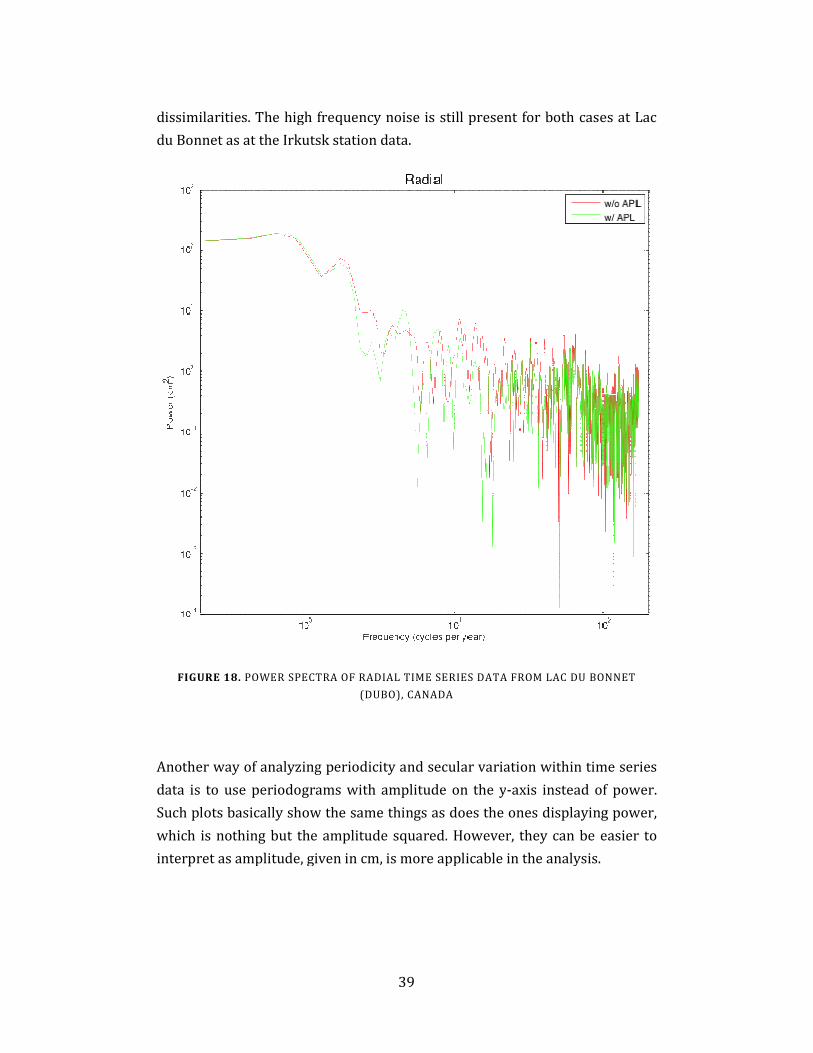
dissimilarities. The high frequency noise is still present for both cases

du Bonnet as at the Irkutsk station data

FIGURE 18. POWER SPECTRA OF RADIAL TI

Another way of analyzing periodicity and secular variation within time series

data is to use periodograms with amplitude on the y

Such plots basically show the sa

which is nothing but the amplitude squared

interpret as amplitude, given in cm, is more applicable in the analysis.

39

The high frequency noise is still present for both cases

du Bonnet as at the Irkutsk station data.

SPECTRA OF RADIAL TIME SERIES DATA FROM LAC DU BONNET

(DUBO), CANADA


data is to use periodograms with amplitude on the y-axis instead of power.

Such plots basically show the same things as does the ones displaying power

which is nothing but the amplitude squared. However, they can be easier to

amplitude, given in cm, is more applicable in the analysis.

The high frequency noise is still present for both cases at Lac

LAC DU BONNET


axis instead of power.

me things as does the ones displaying power,

. However, they can be easier to

Figure 19 below shows the amplitude periodogram of vertical displacement

time series data from Irkutsk, Russia. The red line symbolizes the case with no

atmospheric pressure loading model and the gree

with the model applied. As for the power periodogram for the same station,

shown previously in Figure

(frequencies around 1 cycle per year) is evident

degradation at frequencies somewhat lower than 3.

FIGURE 19. AMPLITUDE PERIODOGRA

Obvious similarities between power and amplitude periodograms can also be

seen in Figure 20 if compared to what was previously presented in

below shows the amplitude periodogram of vertical displacement


spheric pressure loading model and the green line represent the case

As for the power periodogram for the same station,

Figure 17, the improvement around the annual

(frequencies around 1 cycle per year) is evident, as is the insignificant

degradation at frequencies somewhat lower than 3.

AMPLITUDE PERIODOGRAM OF RADIAL TIME SERIES DATA FROM IRKUTS

(IRKJ), RUSSIA

ties between power and amplitude periodograms can also be

if compared to what was previously presented in

below shows the amplitude periodogram of vertical displacement


n line represent the case

As for the power periodogram for the same station,

, the improvement around the annual

, as is the insignificant

IES DATA FROM IRKUTSK

ties between power and amplitude periodograms can also be

if compared to what was previously presented in Figure

18. The red line continuously represents the case without atmospheric

pressure loading whilst the green line represents the

model is implemented.

FIGURE 20. AMPLITUDE PERIODOGRA

41

. The red line continuously represents the case without atmospheric

pressure loading whilst the green line represents the situation when the

AMPLITUDE PERIODOGRAM OF RADIAL TIME SERIES DATA FROM LAC DU

BONNET (DUBO), CANADA

. The red line continuously represents the case without atmospheric

when the

IES DATA FROM LAC DU

6. DISCUSSION The results show reason to believe that implementing the model of

atmospheric pressure loading will improve the precision of GPS

measurement, especially affecting the vertical component of position vectors.

Nevertheless, there are remaining issues causing noise to interfere with the

measurement data, which may result in deficiencies within the analysis. Such

issues can be divided into three main categories. Firstly, the procedure of the

analysis itself may contain shortcomings. Secondly, the model of atmospheric

pressure loading may be slightly inaccurate and, thirdly, other phenomena

may affect the GPS measurement time series data.

Regarding the analysis, the main issues are most probably associated with the

quite limited number of stations used and the stations’ locations, along with

the fact that daily averages where used for the analysis instead of the original

6-hourly displacement data. All included stations are situated far (>500 km)

from the oceans where the effect of atmospheric pressure loading is likely to

be at its greatest.

As a next step in this process of implementing atmospheric pressure loading

in GIPSY-OASIS, it is suggested to include more stations in the test-runs.

Furthermore, the stations are to be situated closer to the ocean in order to

examine influence from ocean loading. Subsequently, the 6-hourly

displacement data can be used instead of the daily averages to enable analysis

of short-term fluctuations such as tidal effects. The procedure of the analysis,

however, is considered to be consistent and reliable.

The main source of potential disadvantages in this project is the model for

calculating atmospheric pressure loading from meteorological pressure data.

First and foremost, the pressure data provided by NCEP may be inaccurate. As

the global distribution of meteorological stations, at which pressure data is

collected, is uneven with more dense coverage of North America and western

Europe than the rest of the world, the pressure fields created from the

measured data may be inadequate.

Furthermore, the pressure grid is rather coarse (2.5° x 2.5°), which can lead to

insufficiently modeled pressure distributions at some sites, especially in areas

43

with lots of local variations for example in mountainous regions. Neither is the

grid fine enough to account for variations of the rock or soil structures

underlying the GPS stations. A station located on soft clay is more likely to be

affected by atmospheric pressure loading than is a station situated on

extensive igneous rock.

It is possible that the Green’s functions used in the model for computing

loading distribution from atmospheric surface pressure contain inadequacies.

Assessments found in literature solely compare the specific functions used in

this project to other Green’s functions, arguing only that the used Green’s

functions are better than their “rival” in the assessments. It does not, in fact,

prove that the fundamental physical assumptions, on which all Green’s

functions are based, are accurate. It is possible that the effects of atmospheric

pressure loading are, in some cases, overestimated by the model.

Another difficulty in connection to this project is the fact that atmospheric

pressure loading is not the only phenomena bringing noise to GPS

measurement data. Also other signals, which may interfere with the

atmospheric loading effects, are present. How well a certain effect is modeled

is hard to tell, especially if other phenomena interfere destructively and the

effects add each other out. If that is the case, applying a model of only one of

the effects could cause more harm than benefit.

Moreover, other phenomena than atmospheric pressure loading are causing

crustal deflections. For example, variations in water storage at lakes and in

the underlying soil have proven to result in movements on the surface of the

Earth. Such effects can be both random and follow trends, as precipitation and

water storage volume generally is seasonally dependant. Some stations

included in the analysis are situated in the vicinity of seas and lakes of

considerable sizes and may thus be subject to such effects.

7. CONCLUSIONS Crustal movements caused by variations in atmospheric pressure are found to

affect the accuracy of high precision GPS measurement. By applying a model

of the deflections, it is possible to reduce the effects and thus enhance the

accuracy. In this Master of Science thesis, an evaluation of the effects from

applying such a model is presented.

The model uses NCEP (National Centers for Environmental Prediction)

reanalysis pressure data to calculate crustal movements by convolving

Green’s functions according to Farrell (1972). Pressure data is collected at 6-

hourly intervals over a 2.5° x 2.5° grid. Displacement time series are created

from high precision GPS measurements at 29 GPS stations located more than

500 km inland. The model of atmospheric pressure loading is applied on the

time series in terms of daily average values, derived from the 6-hourly data, in

order to avoid influence from diurnal and semi-diurnal variations.

Subsequently, the two sets of time series; the original data without the model

(1), and after having applied the model (2), where analyzed by comparing

data scatter and periodicity.

Results of the analysis show that measurement data scatter can be reduced by

implementing the model. The largest reductions are found in the radial

direction, whilst generally only insignificant effects are found in the longitude.

Statistical analysis shows that data scatter in the latitudinal direction is

somewhat degraded, but the effects are very small compared to those in the

radial. In average, the variance within the time series data scatter was

reduced by ~28 % for the vertical component, increased by ~6% for the

latitude and unaffected (~0 % change) for the longitude.

Spectral analysis with periodogram indicate that for most stations, the largest

benefits from applying the model for atmospheric pressure loading are found

at low (around annual) frequencies. At some stations, however, the most

significant reductions are found at mid-frequencies, proving that local

environment determines the nature of the loading response.

In conclusion, results show positive effects of implementing the atmospheric

pressure loading model. However, further analysis is needed before including

45

the model in GIPSY-OASIS GPS data processing procedure. As a next step, it is

recommended that more stations are included, situated closer to the oceans in

order to investigate how well the oceanic response is modeled. Furthermore,

the original 6-hourly data is suggested to be included instead of daily

averages, to enable sub-daily variation.

8. REFERENCES Dziewonski, A. M., & Anderson, D. L. (1981). Preliminary reference Earth

model. Physics of The Earth and Planetery Interiors , 25 (4), 297 - 356.

Farrell, W. E. (1972). Deformation of the Earth by Surface Loads. Reviews of

Geophysics and Space Physics , 10 (3), 761 - 797.

Gregorius, T. (1996). GIPSY-OASIS II: How it works... Newcastle: Department of

Geomatics, University of Newcastle upon Tyne.

Gutner, W. (2002 йил 25-01). SWEPOS. Retrieved 2010 йил 17-05 from

RINEX: The Receiver Independent Exchange Format Version 2.10:

http://swepos.lmv.lm.se/rinex/rinex210.txt

IGS Central Bureau. (2007 йил 26-07). IGS Central Guidelines. Retrieved 2010

йил 01-06 from International GNSS Service:

http://igscb.jpl.nasa.gov/network/guidelines/guidelines.html#allsites

Jet Propulsion Laboratory. (2008). Introduction to gd2p.pl. GIPSY User Group

Meeting/Class. Pasadena, CA: JPL.

Jet Propulsion Laboratory. (2010). Introduction to GIPSY Software. Pasadena,

CA: California Institute of Technology.

Newport, B. (2006). User's Guide GPS Network Processor Version 3.0. Pasadena:

Jet Propulsion Laboratory.

NOAA. (2007 йил 23-08). About NCEP. Retrieved 2010 йил 12-07 from

National Centers for Environmental Prediction:

http://www.ncep.noaa.gov/about/

Petrov, L. (2008 йил 01-11). Atmospheric Pressure Loading Service. Retrieved

2010 йил 19-07 from The Goddard Geodetic VLBI Group's Gemini auxiliary

web pages: http://gemini.gsfc.nasa.gov/aplo/

Petrov, L., & Boy, J.-P. (2004). Study of the atmospheric pressure loading

signal in very long baseline interferometry observations. Journal of

Geophysical Research , 109.

47

Seeber, G. (1993). Satellite geodesy : foundations, methods, and applications.

Berlin ; New York: Walter de Gruyter & Co.

U.S. National Executive Committee for Space-Based Positioning, Navigation

and Timing. (2009 йил 28th-May). The Global Positioning System. Retrieved

2010 йил 5th-May from Space-Based Positioning, Navigation & Timing:

http://www.gps.gov/

van Dam, T. M., Blewitt, G., & Heflin, M. B. (1994). Atmospheric pressure

loading effects on Global Positioning System coordinate determinations.

Journal of Geophysical Research , 99 (23), 939 - 950.

van Dam, T., Altamimi, Z., Collilieux, X., & Ray, J. (2009). Topographically

Induced Height Errors in Predicted Atmospheric Loading Effects. Faculte des

Sciences de la Technologie et de la Communication. Luxembourg: University

of Luxembourg.

Wells, D., Beck, N., Delikaraoglou, D., Kleusberg, A., Krakiwsky, E. J., Lachapelle,

G., et al. (1986). Guide to GPS Positioning. Fredericton, N.B., Canada: Canadian

GPS Associated.

Wunsch, C., & Stammer, D. (1997). Atmospheric Loading and the oceanic

"Inverted Barometer" Effect. Reviews of Geophysics , 35, 117 - 135.

APPENDIX A

49

APPENDIX B

Vertical displacements, ur, are computed with the following formulae,

according to Farrell (1972) and Petrov and Boy (2004):

ur(r, t) = ∆P(r', t)GR (ψ)cosϕ'dλ'dϕ'∫∫

where, r is the site coordinates

t is the time

ΔP is the variation in surface pressure

GR is the vertical Green’s function (see below)

ψ is the angular distance between the station with coordinates r and

the pressure source with coordinates r’

φ’ is the geocentric latitude and

λ’ is the longitude

The vertical Green’s function is:

GR (ψ) =fa

g0

2h'n Pn (cosψ)

n =0

+∞

∑

where, f is the universal constant of gravitation (as defined in PREM)

a is the Earth’s radius (as defined in PREM)

g0 is the mean surface gravity (as defined in PREM)

hn’ is a computed Love number and

Pn is the Legendre polynomial of degree n

Horizontal displacements, uh, are computed with the following formulae:

uh (r, t) = q(r,r')∆P(r', t)GH (ψ)cosϕ'dλ'dϕ'∫∫

where, q(r,r’) is the unit vector originating from the station, tangential to the

Earth’s surface and

GH is the tangential Green’s function (see below)

GH (ψ) = −fa

g0

2l'n

∂Pn (cosψ)

∂ψn =1

+∞

∑

where, l’n is a computed Love number

evaluation of atmospheric pressure loading effects on gps

Documents