evaluation of chiller modeling approaches …gaia.lbl.gov/btech/papers/48856.pdf · statistical...
TRANSCRIPT
LBNL-48856
CD-485
This work was completed under contract to Lawrence Berkeley National Laboratory as part of the High Performance Commercial Building Systems program. This program is supported by the California Energy Commission's Public Interest Energy Research (PIER) Buildings Program and the Assistant Secretary for Energy Efficiency and Renewable Energy, Office of Building Technology, Building Technologies Program, of the U.S. Department of Energy under Contract No. DE-AC03-76SF00098.
EVALUATION OF CHILLER MODELING APPROACHES AND THEIR USABILITY
FOR FAULT DETECTION
Prepared by:
Priya Sreedharan Department of Mechanical Engineering, University of California, Berkeley and
Commercial Buildings Group, Building Technologies Department
Environmental and Energy Technologies Division Ernest Orlando Lawrence Berkeley National Laboratory
1 Cyclotron Road Berkeley, California 94720
MASTERS PROJECT (PLAN II)
Reviewed by:
Professor Van P. Carey, Professor David M. Auslander
Department of Mechanical Engineering,
University of California, Berkeley
May 2001

Masters Project – Plan II i Priya Sreedharan
TABLE OF CONTENTS
1. ABSTRACT ........................................................................................................................... 1
2. INTRODUCTION ................................................................................................................... 2 2.1 PROJECT GOAL......................................................................................................... 2 2.2 BRIEF DESCRIPTION OF FAULT DETECTION AND DIAGNOSIS .................................... 2 2.3 CATEGORIES OF MODELS ......................................................................................... 3 2.4 APPROACHES TO MODELING IN HVAC&R SYSTEMS ............................................. 3 2.5 MODELING CONSIDERATIONS .................................................................................. 4 2.6 SELECTED MODELS .................................................................................................. 4
3. OVERVIEW OF VAPOR COMPRESSION CHILLER MODELS ................................................ 6 3.1 PHYSICAL COMPONENT MODELS ............................................................................. 6 3.2 PHYSICAL PARAMETER ESTIMATION MODELS ......................................................... 9 3.3 ARTIFICIAL NEURAL NETWORKS ........................................................................... 10 3.4 POLYNOMIAL CURVE FITTING................................................................................ 10
4. ASHRAE PRIMARY TOOLKIT COMPONENT CHILLER MODEL ..................................... 12 4.1 INTRODUCTION....................................................................................................... 12 4.2 COMPONENT BY COMPONENT ................................................................................ 12 4.3 COMPUTATIONAL SCHEME - FULL LOAD OPERATION............................................ 16 4.4 PART LOAD VARIATIONS ....................................................................................... 17 1.5 CALIBRATION OF ORIGINAL TOOLKIT MODEL ....................................................... 17 4.6 MODIFICATIONS TO THE MODEL AND COMPUTATIONAL SCHEME .......................... 18 4.7 CALIBRATION OF MODIFIED TOOLKIT MODEL ....................................................... 20
5. GORDON-NG UNIVERSAL CHILLER MODEL.................................................................... 24 5.1 INTRODUCTION....................................................................................................... 24 5.2 DESCRIPTION AND CALIBRATION ........................................................................... 24 5.3 COMPARISON BETWEEN TOOLKIT AND GORDON-NG MODELS.............................. 25
6. EMPIRICAL MODEL (DOE-2/COOLTOOLS)...................................................................... 27 6.1 INTRODUCTION....................................................................................................... 27 6.2 DESCRIPTION.......................................................................................................... 27 6.3 CALIBRATION......................................................................................................... 28
7. MEASURED DATA AND DATA PROCESSING...................................................................... 30 7.1 LABORATORY CHILLER .......................................................................................... 30 7.2 FIELD (BUILDING) CHILLER ................................................................................... 31
8. UNCERTAINTY ANALYSIS ................................................................................................. 34 8.1 EVAPORATOR AND CONDENSER LOAD UNCERTAINTIES......................................... 34 8.2 UNCERTAINTY IN MODELED PREDICTIONS............................................................... 35

Masters Project – Plan II ii Priya Sreedharan
9. RESULTS – LABORATORY CASE STUDY........................................................................... 37 9.1 ENERGY BALANCE AND UNCERTAINTY IN LOAD CALCULATIONS.......................... 37 9.2 ASHRAE TOOLKIT RESULTS................................................................................. 42 9.3 GORDON-NG UNIVERSAL MODEL RESULTS ........................................................... 49 9.4 DOE-2 MODEL RESULTS ....................................................................................... 53
10. RESULTS – FIELD CASE STUDY ............................................................................ 60 10.1 DATA PROCESSING................................................................................................. 60 10.2 ASHRAE TOOLKIT RESULTS................................................................................. 64 10.3 GORDON-NG UNIVERSAL MODEL RESULTS ........................................................... 68 10.4 COOLTOOLS/DOE-2 MODEL RESULTS .................................................................. 73
11. DISCUSSION........................................................................................................... 77 11.1 SUMMARY OF RESULTS AND GENERAL OBSERVATIONS......................................... 77 11.2 MODEL LIMITATIONS ............................................................................................. 79 11.3 BUILDING CHILLER MODEL PREDICTION DISCONTINUITY ..................................... 80
12. CONCLUSIONS ....................................................................................................... 85
ACKNOWLEDGEMENTS ............................................................................................................. 1
REFERENCES............................................................................................................................. 2

Masters Project – Plan II iii Priya Sreedharan
LIST OF TABLES
TABLE 4.1. LIST OF SYMBOLS .............................................................................................................. 14
TABLE 5. 1. COMPARISON OF PHYSICAL MODELS ............................................................................... 26
TABLE 7.1: SENSORS AND UNCERTAINTY............................................................................................ 31
TABLE 7.2: SENSORS AND UNCERTAINTY............................................................................................ 32
TABLE 9.1 PARAMETER ESTIMATION RESULTS ................................................................................... 42
TABLE 9.2. STATISTICAL ANALYSIS OF TOOLKIT MODEL RESULTS ................................................... 46
TABLE 9.3. STATISTICAL ANALYSIS OF GORDON-NG MODEL RESULTS ............................................. 52
TABLE 9.4. DOE-2 PARAMETERS AND REFERENCE CONDITIONS – ADJUSTED POWER DATA ........... 53
TABLE 9.5. DOE-2 PARAMETERS AND REFERENCE CONDITIONS – ORIGINAL POWER DATA ............ 56
TABLE 9.6. STATISTICAL ANALYSIS OF DOE-2 MODEL RESULTS ...................................................... 58
TABLE 10.1 PARAMETER ESTIMATION RESULTS ................................................................................. 65
TABLE 10.2. STATISTICAL ANALYSIS OF TOOLKIT MODEL RESULTS – BINNED DATA SET ............... 66
TABLE 10.3. STATISTICAL ANALYSIS OF TOOLKIT MODEL RESULTS – UNBINNED, FILTERED DATA
SET .......................................................................................................................................... 67
TABLE 10.4. STATISTICAL ANALYSIS OF GORDON-NG MODEL RESULTS – BINNED DATA SET ......... 71
TABLE 10.5. STATISTICAL ANALYSIS OF GORDON-NG MODEL RESULTS- FULL DATA SET............... 72
TABLE 10.5. COOLTOOLS AUTOMATED CALIBRATION PARAMETERS AND REFERENCE CONDITIONS 73
TABLE 10.6. STATISTICAL ANALYSIS OF COOLTOOLS/DOE-2 MODEL RESULTS- AUTOMATED
CALIBRATION (BINNED DATA SET) ........................................................................................ 74
TABLE 10.7. STATISTICAL ANALYSIS OF COOLTOOLS/DOE-2 MODEL RESULTS- FULL (UNBINNED & FILTERED) DATA SET.............................................................................................................. 75
TABLE 11.1 SUMMARY OF MODELING RESULTS ................................................................................. 77

Masters Project – Plan II iv Priya Sreedharan
LIST OF FIGURES
FIGURE 2.1. MODEL BASED FAULT DETECTION OVERVIEW ................................................................. 2
FIGURE 9.1. ENERGY BALANCE .......................................................................................................... 37
FIGURE 9.2. ENERGY BALANCE AS PERCENTAGE OF MAXIMUM POWER............................................ 38
FIGURE 9.3. ENERGY BALANCE AS PERCENTAGE OF MAXIMUM EVAPORATOR LOAD ....................... 38
FIGURE 9.4. ENERGY BALANCE CORRELATION WITH EVAPORATOR LOAD ...................................... 39
FIGURE 9.5. ENERGY BALANCE CORRELATION WITH CONDENSER LOAD......................................... 39
FIGURE 9.6. ENERGY BALANCE CORRELATION WITH COMPRESSOR POWER .................................... 40
FIGURE 9.7 ENERGY BALANCE (% MAXIMUM POWER) ..................................................................... 41
FIGURE 9.8 ENERGY BALANCE (% MAXIMUM EVAPORATOR LOAD) ................................................ 41
FIGURE 9.9 ADJUSTED ENERGY BALANCE .......................................................................................... 41
FIGURE 9.10. ASHRAE TOOLKIT RESULTS - LABORATORY CHILLER - OBJECTIVE FUNCTION
(ADJUSTED DATA)................................................................................................................... 43
FIGURE 9.11. ASHRAE TOOLKIT RESULTS - LABORATORY CHILLER - OBJECTIVE FUNCTION
(ORIGINAL DATA) ................................................................................................................... 44
FIGURE 9.12. ASHRAE TOOLKIT RESULTS - LABORATORY CHILLER (ADJUSTED DATA)................ 45
FIGURE 9.13. ASHRAE TOOLKIT RESULTS - LABORATORY CHILLER (ORIGINAL DATA)................. 45
FIGURE 9.14. EVAPORATOR PRESSURE MODEL PREDICTIONS (ORIGINAL DATA) ............................. 46
FIGURE 9.15. CONDENSER PRESSURE MODEL PREDICTIONS (ORIGINAL DATA)................................ 47
FIGURE 9.16. ASHRAE TOOLKIT RESULTS - LABORATORY CHILLER WITH UNCERTAINTY ERROR
BARS (ORIGINAL DATA) ......................................................................................................... 48
FIGURE 9.17. ASHRAE TOOLKIT CONDENSER LOAD PREDICTIONS- LABORATORY CHILLER .......... 49
FIGURE 9.18. GORDON-NG LINEAR REGRESSION RESULTS (ADJUSTED POWER) .............................. 50
FIGURE 9.19. GORDON-NG LINEAR REGRESSION RESULTS (ORIGINAL POWER) ............................... 50

Masters Project – Plan II v Priya Sreedharan
FIGURE 9.20. GORDON-NG MODEL RESULTS - LABORATORY CHILLER (ADJUSTED DATA) ............. 51
FIGURE 9.21. GORDON-NG MODEL RESULTS - LABORATORY CHILLER (ORIGINAL DATA) .............. 51
FIGURE 9.22. GORDON-NG MODEL RESULTS WITH UNCERTAINTY ERROR BARS - LABORATORY
CHILLER .................................................................................................................................. 53
FIGURE 9.23. DOE-2 CALIBRATION OF CAPFT CURVE - LABORATORY CHILLER (ADJUSTED DATA)54
FIGURE 9.24. DOE-2 CALIBRATION OF EIRFT CURVE - LABORATORY CHILLER (ADJUSTED DATA)54
FIGURE 9.25. DOE-2 CALIBRATION OF EIRFPLR CURVE - LABORATORY CHILLER (ADJUSTED
DATA)...................................................................................................................................... 55
FIGURE 9.26. DOE-2 RESULTS - LABORATORY CHILLER (ADJUSTED DATA).................................... 55
FIGURE 9.27. DOE-2 CALIBRATION OF CAPFT CURVE - LABORATORY CHILLER (ORIGINAL DATA)56
FIGURE 9.28. DOE-2 CALIBRATION OF EIRFT CURVE - LABORATORY CHILLER (ORIGINAL DATA)57
FIGURE 9.29. DOE-2 CALIBRATION OF EIRFPLR CURVE - LABORATORY CHILLER (ORIGINAL
DATA)...................................................................................................................................... 57
FIGURE 9.30. DOE-2 RESULTS - LABORATORY CHILLER (ORIGINAL DATA) ..................................... 58
FIGURE 9.31. DOE-2 MODEL RESULTS WITH UNCERTAINTY ERROR BARS - LABORATORY CHILLER59
FIGURE 10.1. EFFICIENCY - BUILDING CHILLER - ENTIRE FILTERED UNBINNED DATA SET .............. 60
FIGURE 10.2. EFFICIENCY - BUILDING CHILLER – FILTERED BINNED DATA SET ............................... 61
FIGURE 10.3. ENERGY BALANCE - BUILDING CHILLER FILTERED (UNBINNED) DATA....................... 61
FIGURE 10.4. ENERGY BALANCE VS. EVAPORATOR LOAD - BUILDING CHILLER BINNED DATA ....... 62
FIGURE 10.5. ENERGY BALANCE VS. COMPRESSOR POWER - BUILDING CHILLER BINNED DATA ..... 62
FIGURE 10.6. ENERGY BALANCE (% OF MAXIMUM POWER) - BUILDING CHILLER BINNED DATA.... 63
FIGURE 10.7. ENERGY BALANCE (% OF MAXIMUM EVAPORATOR LOAD) - BUILDING CHILLER
BINNED DATA ......................................................................................................................... 63
FIGURE 10.9. ASHRAE TOOLKIT RESULTS - BUILDING CHILLER - OBJECTIVE FUNCTION .............. 65
FIGURE 10.10. ASHRAE TOOLKIT RESULTS - BUILDING CHILLER ................................................... 66
FIGURE 10.11. ASHRAE TOOLKIT RESULTS - BUILDING CHILLER FILTERED UNBINNED DATA SET67
FIGURE 10.12. ASHRAE TOOLKIT RESULTS WITH UNCERTAINTY ERROR BARS - BUILDING CHILLER68

Masters Project – Plan II vi Priya Sreedharan
FIGURE 10.13. GORDON-NG LINEAR REGRESSION RESULTS - BUILDING CHILLER ........................... 69
FIGURE 10.14. GORDON-NG MODEL RESULTS - BUILDING CHILLER BINNED DATA SET.................. 71
FIGURE 10.15. GORDON-NG MODEL RESULTS - BUILDING CHILLER FILTERED UNBINNED DATA SET72
FIGURE 10.16. GORDON-NG MODEL RESULTS WITH UNCERTAINTY ERROR BARS -BUILDING
CHILLER .................................................................................................................................. 73
FIGURE 10.17. COOLTOOLS/DOE-2 RESULTS - BUILDING CHILLER BINNED DATA SET................... 74
FIGURE 10.18. COOLTOOLS/DOE-2 RESULTS - BUILDING CHILLER FILTERED UNBINNED DATA SET75
FIGURE 10.19. COOLTOOLS/DOE-2 RESULTS WITH UNCERTAINTY ERROR BARS - BUILDING
CHILLER .................................................................................................................................. 76
FIGURE 11.7. RESIDUAL VS. TEMPERATURE LIFT – BUILDING CHILLER BINNED DATA..................... 80
FIGURE 11.8. RESIDUAL VS. ENERGY BALANCE – BUILDING CHILLER BINNED DATA....................... 81
FIGURE 11.9. MEASURED EFFICIENCY – BUILDING CHILLER BINNED DATA...................................... 82
FIGURE 11.1. RESIDUAL ANALYSIS – GORDON-NG MODEL RESULTS - BUILDING CHILLER FILTERED
DATA ....................................................................................................................................... 83
FIGURE 11.2. RESIDUAL ANALYSIS - EFFICIENCY - BUILDING CHILLER FILTERED DATA................. 83

Masters Project – Plan II 1 Priya Sreedharan
1. ABSTRACT
Selecting the model is an important and essential step in model based fault detection and diagnosis (FDD). Several factors must be considered in model evaluation, including accuracy, training data requirements, calibration effort, generality, and computational requirements. All modeling approaches fall somewhere between pure first-principles models, and empirical models. The objective of this study was to evaluate different modeling approaches for their applicability to model based FDD of vapor compression air conditioning units, which are commonly known as chillers. Three different models were studied: two are based on first-principles and the third is empirical in nature. The first-principles models are the Gordon and Ng Universal Chiller model (2nd generation), and a modified version of the ASHRAE Primary Toolkit model, which are both based on first principles. The DOE-2 chiller model as implemented in CoolToolsTM was selected for the empirical category. The models were compared in terms of their ability to reproduce the observed performance of an older chiller operating in a commercial building, and a newer chiller in a laboratory. The DOE-2 and Gordon-Ng models were calibrated by linear regression, while a direct-search method was used to calibrate the Toolkit model. The "CoolTools" package contains a library of calibrated DOE-2 curves for a variety of different chillers, and was used to calibrate the building chiller to the DOE-2 model. All three models displayed similar levels of accuracy. Of the first principles models, the Gordon-Ng model has the advantage of being linear in the parameters, which allows more robust parameter estimation methods to be used and facilitates estimation of the uncertainty in the parameter values. The ASHRAE Toolkit Model may have advantages when refrigerant temperature measurements are also available. The DOE-2 model can be expected to have advantages when very limited data are available to calibrate the model, as long as one of the previously identified models in the CoolTools library matches the performance of the chiller in question.

Masters Project – Plan II 2 Priya Sreedharan
2. INTRODUCTION
2.1 PROJECT GOAL
The ability to detect faults in equipment can result in reduced energy, maintenance costs, and extended equipment life. Model based fault detection begins with selecting a model of the physical system. This project evaluated various models for vapor compression refrigeration units (commonly known as chillers). The models were compared using various criteria such as prediction accuracy, calibration effort, and training data requirements, usefulness of parameters, computational requirements, and generality of the model. Fault detection and diagnostics (FDD) and various modeling approaches are described in more detail in this section.
2.2 BRIEF DESCRIPTION OF FAULT DETECTION AND DIAGNOSIS
The field of fault detection and diagnosis (FDD) applied to heating, ventilating, air conditioning and refrigerating (HVAC&R ) systems is relatively new. Interest in the HVAC&R field has lagged behind others, primarily because of the high cost to benefit ratio, compared to other industries. (Braun, 1999). Within engineering fields, it first originated in the chemical and nuclear industries. In these industries, the driving forces have primarily been safety and quality control. Within mechanical engineering, it has been applied to automotive, fluid, combustion and HVAC&R systems (Issermann, 1997). FDD involves two steps: detecting that a fault is present, then isolating and diagnosing it. Faults can be classified as either degradation or abrupt faults. In HVAC&R systems, an example of a degradation fault is the gradual leakage of refrigerant from an air conditioning unit, which increases energy use. An abrupt fault could be the failure of a sensor, or the breaking of a fan belt. These faults, unlike degradation faults, are immediately detectable. FDD can be as simple as monitoring and comparing sensor readings to a threshold. Model-based FDD automates the fault detection process, reducing the need for manual inspection of performance data. Figure 2.1 describes the general process of model-based fault detection:
Figure 2.1. Model Based Fault Detection Overview
RealSystem
ModeledSystem
Inputs(measurements)
Real Output
Modeled Output
-
+
Residual >threshold ?

Masters Project – Plan II 3 Priya Sreedharan
The inputs are sensor measurements or control signals. The model processes the measured data and generates an output, which is then compared to the actual output from the system. Residuals, or innovations beyond a pre-determined threshold indicate the presence of a fault. The selection of the model is an important step, that governs the accuracy of fault detection. This project focused on the selection of a model for FDD of water cooled vapor compression refrigeration units, commonly known as chillers. Specifically, three models were studied to assess their applicability to model-based FDD of chillers.
2.3 CATEGORIES OF MODELS
Models can be classified into two broad classes: empirical (black-box), and analytical (physical or first principles). Empirical models do not incorporate any kind of prior knowledge of the system. Examples of empirical models include polynomial curve fits, and artificial neural networks. An advantage of empirical models is that detailed physical knowledge of the system is not necessary. A disadvantage is that the model is reliable only for operating points within the range of the training data, and extrapolation outside this range may lead to significant error. In order to properly train the model, adequate training data are required; the richer the data, the more accurate the model predictions. Analytical or physical models, also known as white-box models are largely based on the laws of physics. Physical models may require less training data, since the model should be valid at all operating conditions for which the assumptions inherent in the model are valid. A disadvantage is that a good understanding of the physical phenomena is necessary for an accurate model, which is not always available. It is nearly impossible to model a system perfectly, and in addition, ‘unmodeled disturbances’ contribute to the inaccuracy of the model. In practice, a model may be partly empirical, and partly based on first principles. (Haves, 1999)
2.4 APPROACHES TO MODELING IN HVAC&R SYSTEMS
There are two main approaches to model-based FDD of HVAC&R systems: the whole building (top-down) level approach, and component level (bottom-up) approach. The whole building approach focuses on the energy consumption of the whole building, and major systems (such as chilled water, lighting, fans). Actual energy consumption is compared to the expected consumption, based on a whole building simulation program1. The component level approach focuses on modeling individual pieces of equipment, or local systems. Actual performance is compared to the baseline performance, which is the model predictions based on either manufacturer's data, or training data acquired during correct operation. In actual implementation, an FDD scheme may link the two approaches. While the whole-building approach may be more simple, it is not sufficient to localize the actual fault. The component level
1 Such as the DOE-2, or Energy-Plus simulation programs developed by Lawrence Berkeley National Laboratory.

Masters Project – Plan II 4 Priya Sreedharan
approach has the advantage of relating the faults to a specific piece of equipment or system, but is a more complex approach. (Haves, 1999)
2.5 MODELING CONSIDERATIONS
The selection of a model is based on a variety of factors. Eventually, these techniques will be deployed in commercial buildings, with the intent to save energy, and improve occupant comfort. With this in mind, the following factors should be considered in the selection of the model: ¾ accuracy ¾ calibration effort and training data requirements ¾ computational scheme ¾ physical relevance of parameters (for physical models) As with any kind of model, accuracy is important. Moreover, in FDD applications, it is important that 'false alarms' are not generated. That is, the detection routine must be robust such that only real faults are detected. This requires that the model is able to predict operation within small error. Calibration of the model is a critical step. The more limited the range of conditions for which training data are required, the more quickly and easily these data can be obtained. Unlike in a laboratory setting, existing building equipment cannot be tested at will. Although computational load is not usually a problem, the estimation of the values of the parameters of a model that is both non-linear in the inputs and non-linear in the parameters can be both slow and uncertain. When physical models are used, the parameters obtained through calibration should be physically meaningful. For example, if their values suggest the presence of a fault, not only is a fault detected, but the cause of the fault may be more easily identified.
2.6 SELECTED MODELS
The objective of this study was to validate various chiller models using operating data from real chillers. The three following steady-state chiller models were selected for this study: 1) ASHRAE Primary HVAC&R Toolkit Model (Bourdouxhe et al. 1997) 2) Gordon-Ng Universal Chiller Model (Ng et al. 1997) 3) CoolTools/ (DOE-2) Model (Pacific Gas and Electric, 1996) The first two models were selected because they are both physical models, and differ in their formulation and structure. The Primary Toolkit model is a component model, which is based on thermodynamic (first law) and heat transfer relationships, whose equations are solved in an iterative manner. The Gordon-Ng Universal model is based on both the first and second laws of thermodynamics, and uses heat transfer relationships as well. However, it is not a component model, but uses a systems approach, and the model structure provides a simple, explicit solution. The DOE-2 model is an empirical model based on polynomial curve fits, which relate the efficiency, capacity, and energy consumption to the operating conditions.

Masters Project – Plan II 5 Priya Sreedharan
At this point, it is useful to distinguish between steady-state and transient models. The models selected are all steady-state models, and could not be applied to data obtained during transient operation. Examples of transient operation are start-up and shutdown. Mathematically, steady-state models consist of algebraic equations, while transient models consist of differential equations. The model selection was limited by the kind of measurements and information available for the chillers studied. For example, detailed heat exchanger dimensions were not available for the building chiller. Refrigerant temperature and pressure measurements were also unavailable for the building chiller, and are not generally available on-line, although this is slowly changing.

Masters Project – Plan II 6 Priya Sreedharan
3. OVERVIEW OF VAPOR COMPRESSION CHILLER MODELS
The objective of this study was to compare various types of vapor compression chiller models for the purpose of fault detection and diagnosis. Fault detection and diagnosis (FDD) as a general subject is vast. It was determined that a thorough literature review of this subject is not only a challenging endeavor, but outside the scope of this study. Therefore, this section is limited to a discussion of the types of chiller models, and if applicable, their use in fault detection schemes. Section 2.3 briefly described the broad approaches to modeling, which included first-principles or physical models, and empirical models. The next few sections describe four different chiller modeling approaches, two within each of these categories. The physical component modeling section is by no means comprehensive in the various nuances to compressor and heat exchanger modeling, but is intended to give a flavor of the issues and general approaches to component modeling.
3.1 PHYSICAL COMPONENT MODELS
3.1.1 OVERVIEW
In general, the chiller component modeling approach considers each component in the refrigeration cycle and applies mass, momentum and energy balances. Browne et. al (1998) reviewed the existing approaches to steady state and transient chiller modeling (physical). No transient chiller models were found, which remains to be an unsolved problem for the HVAC industry. Various steady-state modeling approaches along with their limitations were discussed in the paper, and are summarized below. COMPRESSORS: In general, compression is assumed to be polytropic2, and the motor is considered to be constant speed. The volumetric efficiency, which is assumed constant, or based on manufacturer’s data, and inlet conditions were used to calculate mass flow rate. Alternatively, an isentropic efficiency is assumed to determine outlet conditions. In a simpler approach, manufacturer-supplied empirical curve fits are used for component models. More complex models consider heat losses and gains through the compressor shell, motor efficiencies, and pressure drops through the intake and exit valves. HEAT EXCHANGERS: The majority of chillers contain an evaporator and condenser of a shell and tube configuration, with the water in the tube, and refrigerant in the shell. The tube may have multiple passes. Traditionally, an effectiveness, or NTU method has been used. The effectiveness is defined as ratio of actual heat transfer to the maximum amount of heat transfer that would occur, if the heat exchanger has infinite surface area. Often, an isothermal heat exchanger is used.3 However, it is limited to the phase-change regions. A more accurate approach assumes separate overall-heat transfer coefficients for the superheating (evaporator), desuperheating, and subcooling (condenser) regions.
2 pvn=constant 3 ε = 1-e-NTU

Masters Project – Plan II 7 Priya Sreedharan
This approach treats the heat exchanger as two (evaporator) or three (condenser) variable sized heat exchangers, of which the total area is known. Another common approach is the log mean temperature difference (LMTD) method, where the heat transfer is the product of the LMTD, overall heat transfer coefficient and area.4
fluid.colder theof res temperatuexiting and entering theare T ,T
and fluid,hot theof res temperatuexiting and entering theare T ,T
,
)(
)(ln
LMTD
coci
hohi
where
TT
TT
)T(T)T(T
ciho
cohi
cohiciho
−−
−−−=
This approach is a good representation of a classical heat exchanger if both superheating and evaporation are considered in the evaporator, and likewise, desuperheating, condensation, and subcooling are considered in the condenser. In counterflow heat exchangers, the heat exchanger can be divided into the various regions of heat transfer; then the overall heat transfer coefficients for each region can be determined. In shell and tube heat exchangers, these different regions are not well defined. If the evaporator is assumed to include only evaporation, then the LMTD expression is further simplified. Mathematically, the relationship between heat transfer and the overall heat transfer coefficients are identical, however the difference appears in how they are used to estimate the heat transfer coefficients. Normally, the NTU method uses convection correlations to estimate directly the overall heat transfer coefficients; the LMTD method provides a simple method to estimate the overall heat transfer coefficient using fluid temperatures, and avoids the details of convection. Lastly, the elemental methods approach divides the heat exchanger into smaller discrete elements, or control volumes, and solves the mass and energy equations for each control volume. This approach is rarely used to model shell and tube heat exchangers. EXPANSION VALVE: The two most common expansion valves used in chillers are float valves and thermostatic expansion valves. While the control mechanisms and geometry differ, the expansion process is universally modeled as an isenthalpic process. Manufacturers’ data can be used to develop empirical models for the mass flow rate. Alternatively, basic fluid mechanics can be used to relate the mass flow rate to the pressure drop cross the valve. SOLVING THE EQUATIONS: Steady state models, which consist of a set of algebraic equations, can be solved in an iterative process. Derivative based techniques, such as newton-raphson method increase the efficiency of the algorithm. (Many equation solving programs are available as well, such as SPARK and Engineering Equation Solver, which automate the iterative process mentioned above.) Transient models requiring the solution to differential equations, can be solved through numerical integration (e.g., Euler method, which is a simple first order method). Three different approaches to component modeling of chiller are discussed below.
4 Q=UA(LMTD)

Masters Project – Plan II 8 Priya Sreedharan
3.1.2 ASHRAE PRIMARY HVAC 1 TOOLKIT
The Toolkit model (Bourdouxhe, 1994), which will be described in more detail later in this report, is a component modeling approach, with some simplifications to the component models. The heat exchangers are treated as “black-boxes”, where the flow configuration, and areas of the heat exchanger are not used to estimate the overall heat transfer coefficients. Rather, the heat transfer coefficients, and other parameters were found during the calibration, and are selected based on finding the best fit values. Each heat exchanger is assumed to only undergo phase change, neglecting sensible heat transfer. The NTU method was used to estimate heat transfer. The inefficiencies in the compressor are modeled as linearly proportional to the compressor power. These losses, are assumed to sensibly heat the refrigerant. Reciprocating, screw and centrifugal component models are presented for the compressors; the difference between the three is reflected in the parameters used to estimate the volumetric flow rate through the compressor. Expansion is modeled as an isenthalpic process. The Toolkit model, once calibrated, only requires inlet water conditions, and refrigerant property data to predict evaporator load, compressor power, condensing and evaporator pressures, and condenser heat transfer.
3.1.3 PURDUE COMPONENT MODEL APPROACH
A steady state model of a chiller was developed in order to lay the foundation for a dynamic chiller model. (Comstock, 1999, Braun, 2000) Again, the NTU method is used to estimate heat transfer in the heat exchangers. However, the more accurate method, where phase change, and sensible heat transfer are considered separately is employed. The heat transfer coefficients for both the phase change, and sensible heat transfer sections are calculated using the geometry, thermo-physical properties of the fluids, and well known empirical relationships. The area fractions of the different modes of heat transfer are outputs of the model. Using both water measurements, and refrigerant data, the heat transfer, output water temperature, fractional areas for the different modes of heat transfer (i.e., condensing and subcooling, or evaporating and superheating), outlet refrigerant enthalpy, and subcooling/superheating are outputs of the model. The compressor is modeled using both a polytropic and electromechanical efficiency. An empirical relationship is used to relate the polytropic efficiency as a function of power, and the electromechanical efficiency is assumed constant. Expansion was modeled as an isenthalpic process. Each component model is calibrated individually, and an overall system model linked the components, and applied overall energy balances. The overall system model requires only inlet water temperatures and flow rates, and evaporator load (along with refrigerant property data) to predict compressor work, evaporating and condensing pressures, and condenser heat transfer.
3.1.4 ASHRAE PROJECT #1139-RP
The objective of this currently ongoing project is to develop online training methods for model based fault detection in chillers. (Reddy et. al, 2000) Consequently, a variety of chiller models was studied, including a component based modeling approach, which is described here. This approach follows the recommendation of the ASHRAE equipment handbook. The LMTD method is used to estimate the product of the overall heat transfer coefficient and area (UA) for the heat exchangers. The compressor is modeled using a variable electromechanical efficiency, and polytropic efficiency. The polytropic

Masters Project – Plan II 9 Priya Sreedharan
efficiency is dependent, among other things, on empirical relationships obtained from the manufacturer. As usual, the expansion valve is modeled as an isenthalpic process, and is modeled using basic fluid mechanics (i.e., mass flow rate proportional the square root of the pressure differential).
3.2 PHYSICAL PARAMETER ESTIMATION MODELS
The Gordon and Ng models described below are still based on the physics of the refrigeration cycle, but are manipulated into simple linear relationships, for which refrigerant data and thermo-physical properties are not required. In contrast to the previously described component models, the Gordon-Ng models may be regarded as a system models.
3.2.1 GORDON- NG UNIVERSAL CHILLER MODEL (FIRST GENERATION)
The first version of the Gordon and Ng universal chiller model was a physical model with empirical relationships to represent the variation of irreversibility with temperature. It was based on both a system energy and entropy balance. An overall heat exchanger effectiveness was used to relate the refrigerant and water temperatures to the heat transfer in the heat exchangers . Algebraic manipulation resulted in a linear relationship between the inverse of the coefficient of performance (COP) and inverse of the evaporator load. (Gordon, 1995…) Stylianou and Nikanpour (1996) used this model for a reciprocating chiller. The model was used only for fault detection purposes, not fault diagnosis, and for steady state operation. Diagnosis was performed using a rules-based approach. The measured data included condenser and evaporator water temperatures, and compressor power. Brandemuehl (1996) used this model for in-situ testing of chillers. Two centrifugal chillers were tested, and calibrated to the model. The model was used at two levels: the first ignored temperature variations in evaporator and condenser water, and simply regressed the inverse of COP with the inverse of evaporator load. The second mode incorporated the empirical relationships between irreversibility and condenser and evaporator temperatures. It was interesting that these empirical relationships, which had been tested on reciprocating chillers, were able to calibrate data from a centrifugal chiller.
3.2.2 GORDON- NG UNIVERSAL CHILLER MODEL (SECOND GENERATION)
The second generation model, while based on the same concepts, restructured the model such that the parameters found have physical relevance (versus the parameters in the first generation model that are based on an empirical relationship between irreversibility and temperature). The result is a relationship that is linear with these physically meaningful parameters. This model is currently being investigated by the Reddy et. al (Reddy, 2000) as part of ASHRAE project 1139-RP, and was also investigated in this project. More details of the model are given in Section 5.2, however, Gordon and Ng discuss some interesting thermodynamic phenomena of chillers worthy of discussion here (Gordon, 2000). Interestingly, the total internal entropy generation remains constant across different cooling loads, and operating temperatures. An example is in centrifugal chillers, where partial closing of the inlet guide vanes

Masters Project – Plan II 10 Priya Sreedharan
achieves part-load conditions (i.e., lower cooling loads). A qualitative explanation is provided, where the decrease in refrigerant mass flow rate at part-load conditions, is compensated for by an increase in specific entropy generation, such that total entropy generation remains constant. While this is not valid for all chiller types (e.g., it is not valid for thermoelectric chillers, or screw-compressor chillers), it appears to be valid for both reciprocating and centrifugal chillers. This model is discussed in more detail in Section 5.2.
3.3 ARTIFICIAL NEURAL NETWORKS
Comstock (1999) conducted a comprehensive literature search of vapor compression FDD studies, which by necessity included a discussion of the modeling approaches used in the fault detection scheme. Two FDD studies using artificial neural networks were described in this report. In her thesis, Bailey trained artificial neural networks (ANN) using both faulty and faultless data from a screw chiller. The independent variables were fault degree and evaporator load. These were varied to study the effect on the dependent variables: energy consumption, chilled water supply temperature, superheat and subcooling temperatures, suction pressure, and discharge pressure (the latter four were refrigerant data). The faults simulated were refrigerant loss and overcharge, oil loss and overcharge, condenser fouling, and loss of an air-cooled condenser fan. The ability of the neural network to classify these faults was difficult to deduce from the results. The best model presented had a misclassification rate of 20%. Peitsman and Bakker (1996) used autoregressive (ARX) and artificial neural network (ANN) models. The former models are linear in the input data, while the latter combine the input data in a non-linear fashion. The models were trained using laboratory chiller data. Modeling at the system level was used to detect a fault, and models at the component level were used to isolate the fault. The ANN performed slightly better than the ARX in modeling various output conditions, which can be attributed to the non-linearity of the system (i.e., ANN models are better suited to address non-linearity). Only one fault was demonstrated: detecting air in the refrigerant using the discharge refrigerant pressure.
3.4 POLYNOMIAL CURVE FITTING
3.4.1 DOE-2 MODEL
The DOE-2 model was developed by the Department of Energy as a tool to help guide architects, and engineers to design more energy efficient buildings. Within the DOE-2 program is a chiller module that simulates chiller performance. The DOE-2 chiller model (hereafter referred to as DOE-2 model) consists of three polynomial curves. They describe how the cooling capacity of the chiller varies with temperature (inlet evaporator and inlet condenser), how the efficiency (kW/ton) of the chiller varies with temperature, and how the power consumption varies at part load conditions. They are empirical in the sense that the polynomial structure is not based on physical relationships. However, the model is somewhat a grey-box model, since the final power prediction of the chiller is based on physically

Masters Project – Plan II 11 Priya Sreedharan
meaningful quantities obtained from the polynomial curves. An assumption the model makes is that evaporator and condenser water flow rates remain constant. This model was the basis of the CoolTools project, of which the objective was to optimize the operation of chilled water plants. The project included the collection of chiller data from existing buildings for different types of vapor-compression chillers. The DOE-2 model parameters were found for these chillers, and are included in a library of curves contained in the CoolTools software. The CoolTools software, is presented by PG&E as a tool to calibrate the DOE-2 models, and thus predict chiller performance at different operating conditions. (PG&E, 1997). Meyers (1996) calibrated the DOE-2 curves, using manufacturer’s data, and compared the actual performance of the a screw chiller to the expected performance. The DOE-2 model acted as a useful commissioning agent, and helped identify fouling in the condenser water line.

Masters Project – Plan II 12 Priya Sreedharan
4. ASHRAE PRIMARY TOOLKIT COMPONENT CHILLER MODEL
4.1 INTRODUCTION
The Primary HVAC Toolkit is a collection of first principles models for a variety of heat and cooling equipment, such as boilers, various types of vapor-compression chillers, absorption chillers, cooling towers, and gas turbines. The vapor-compression chiller models include algorithms for centrifugal, reciprocating, and screw type compressors. Apart from the differences in the compressor, the remaining components of vapor-compression chillers (hereafter referred to as 'chillers') are similar. These include the expansion device, evaporator and condenser. The chiller model contains four component models, each for the evaporator, compressor, condenser, and expansion device, respectively. In contrast to the other selected models, the ASHRAE Toolkit model was not formulated specifically for the purpose of fault detection and diagnostics work. Rather, the model is used to test the ability of the chiller to reach various chilled (evaporator) water setpoints, and under what control mode, for the given operating conditions. (Bourdouxhe, 1994) That is, for specified inlet condenser and evaporator water temperatures and flow rates, can a particular setpoint be realized, and if so, how much power does the compressor consume; and, is the chiller operating in full-load or part-load conditions? This formulation was not convenient for this project, particularly because the calibration required only full-load data, which was unavailable. The model was restructured, and the computational scheme made more efficient with the secant method. The main physical concepts were retained. The original model, calibration routine, and computational scheme is first described, followed by a description of the modifications made for this study.
4.2 COMPONENT BY COMPONENT
The Toolkit offers several different subroutines. These subroutines differ only in the way they model the compression stage.5 The ideal refrigeration cycle consists of four processes, which are listed with the respective component in brackets. (Cengel, 1994) 1-2 Isentropic compression (Compressor) 2-3 Isobaric desuperheating, phase change from vapor to liquid, and subcooling (Condenser) 3-4 Isenthalpic expansion (Expansion Device) 4-1 Isobaric evaporation, and superheating (Evaporator)
5 Compression depends on the compressor type. For example, the reciprocating compressor models
ideal throttling prior to the compression stage, and ideal throttling after exiting the compressor. The centrifugal compressor only adds throttling prior to compression stage. Furthermore, there are different subroutines based on whether the chiller is at full load, or part load conditions. See the documentation for more detail.

Masters Project – Plan II 13 Priya Sreedharan
The modeling concepts, including the assumptions made are described for each component. Let us first consider full-load operation, that is, the chiller is cooling the evaporator water to the lowest temperature it possibly can. Part-load operation is modeled slightly differently, and is discussed later. COMPRESSOR: Compression, at full load is assumed as isentropic for all compressor types. The electromechanical losses from the motor/transmission system are assumed to be a combination of a constant loss and a loss proportional to the compressor power. These losses are assumed to heat the refrigerant sensibly before it enters the compressor, and are not considered as losses to the environment. In fact, the model assumes that no energy leaks between the refrigerant and the environment. The compressibility factor is used in modeling the refrigerant, which is otherwise treated as an ideal gas. CONDENSER: Heat transfer in the condenser is assumed to be isothermal, that is, the refrigerant only undergoes phase change. Therefore, desuperheating after exiting the compressor as well as subcooling are neglected, and lumped into the isothermal heat transfer phase. The NTU-effectiveness relationship is used to model the heat transfer assuming an infinite capacity on the refrigerant side. The overall heat exchanger effectiveness is one of the parameters determined in the calibration routine. As a result of neglecting the sensible heat transfer, the heat transfer coefficient is artificially inflated. As is common to most heat exchanger analysis, the process is assumed to be isobaric. The refrigerant is assumed to exit at the saturated liquid state. EXPANSION DEVICE: The expansion device assumes an isenthalpic process. This assumption, as described in Section 3, is a common assumption in most chiller models. EVAPORATOR: Like the condenser, heat transfer in the evaporator is modeled as an isothermal process, neglecting superheating prior to compression. The refrigerant is assumed to exit as a saturated vapor. (Bourdouxhe, 1994) Table 4.1 contains a list of symbols used in the model. These symbols will be used consistently throughout the remainder of the report.

Masters Project – Plan II 14 Priya Sreedharan
Table 4.1. List of Symbols
Symbol Description Units Tei Evaporator inlet temperature of water K Teo Evaporator exit temperature of water K Tci Condenser inlet temperature of water K Tco Condenser exit temperature of water K z Ideal gas compressibility factor -- Me Mass flow rate of water through evaporator kg/s Mc Mass flow rate of water through condenser kg/s Cpw Specific heat of water J/kg/K T1 Evaporating temperature of refrigerant (assumed to be isothermal) K T1p Temperature of refrigerant after being superheated by the motor, prior to
compression K
Qe Heat transfer from water to refrigerant in the evaporator J/s P1 Evaporating pressure of refrigerant Pa hfg Enthalpy of vaporization of refrigerant J/kg dhfg Enthalpy of vaporization at the evaporating temperature J/kg h1 Enthalpy of refrigerant exiting evaporator (saturated vapor) J/kg T3 Condensing temperature of refrigerant (assumed to be isothermal) K Qc Heat transfer from refrigerant to water in the condenser J/s P2 Condensing pressure of refrigerant Pa Wlo Constant portion of electromechanical losses of motor W α Portion of electromechanical losses proportional to compressor work -- V Volumetric flow rate of refrigerant through compressor m3/s v1p Specific volume of refrigerant entering compressor m3/kg Mref Mass flow rate of refrigerant kg/s A,B Refrigerant constants in the Clausius Clapeyron equation --, K Tc, Tb, To Refrigerant critical, boiling, and reference temperatures K hfo Enthalpy at reference temperature of the refrigerant J/kg h3 Enthalpy of refrigerant exiting condenser (saturated liquid) J/kg Pcomp Power input to compressor W Win Useful work input to the compressor W Wis Isentropic work input to the compressor W εe Evaporator heat exchanger effectiveness -- εc Condenser heat exchanger effectiveness -- UAe Overall heat transfer coefficient of the evaporator W/K UAc Overall heat transfer coefficient of the condenser W/K

Masters Project – Plan II 15 Priya Sreedharan
4.2.1 COMPONENT EQUATIONS
All component models represented below are universal to all chiller types, but for the compressor volumetric flow rate (4.8), which is dependent on compressor type. (The compressor volumetric flow rate is not shown in detail for this reason.)
( )
)7.4( )(
)6.4(
)5.4(1000
)4.4(1
(4.3) )(
(4.2) or )(
(4.1) )(
:Evaporator
11
1
/1
41
e1e1
e
1
fgopfo
b
bc
cfgfg
TBA
CM
UA
e
refe
pwe
eeipweiee
eoeipwe
dhTTChh
TT
TThdh
eP
e
hhMQ
CM
QTTCMTTQ
TTCMQ
liq
b
pwe
e
+−×+=
−−
×=
×=
−=
−×=
××−=××−=
−××=
+
×−
ε
εε
(4.13) )(
(4.12) )1(
(4.11)
(4.10) v
(4.9) /
(4.8) type)compressor on thedependent is expression (this )(
:Compressor
11
1
1
21
1
11p
1
pvapref
islop
islocomp
k
k
prefis
p
pref
CM
WWTT
WWP
P
PTRzMW
P
TRz
vVM
ParametersCompressorfV
×+
+=
++=
×××=
××=
==
−
αα
Masters Project – Plan II 16 Priya Sreedharan
( )
(4.19) :DeviceExpansion
)18.4( )(
)17.4(1000
)16.4(1
(4.15) or )(
(4.14) )(
:Condenser
34
33
/2
3e3
c
1
hh
TTchh
eP
e
CM
QTTCMTTQ
TTCMQ
opfo
TBA
CM
UA
c
pwcc
ccipwcicc
cicopwc
liq
pwc
c
=
−×+=×=
−=
××+=××−=
−××=
+
×−
ε
εε
In addition, an energy balance on the refrigerant is used. Note, this assumes that all motor losses result in sensible heat transfer to the refrigerant, and therefore, the power to the compressor is considered (rather that useful work input).
(4.20) cQPQ compe =+
4.3 COMPUTATIONAL SCHEME - FULL LOAD OPERATION
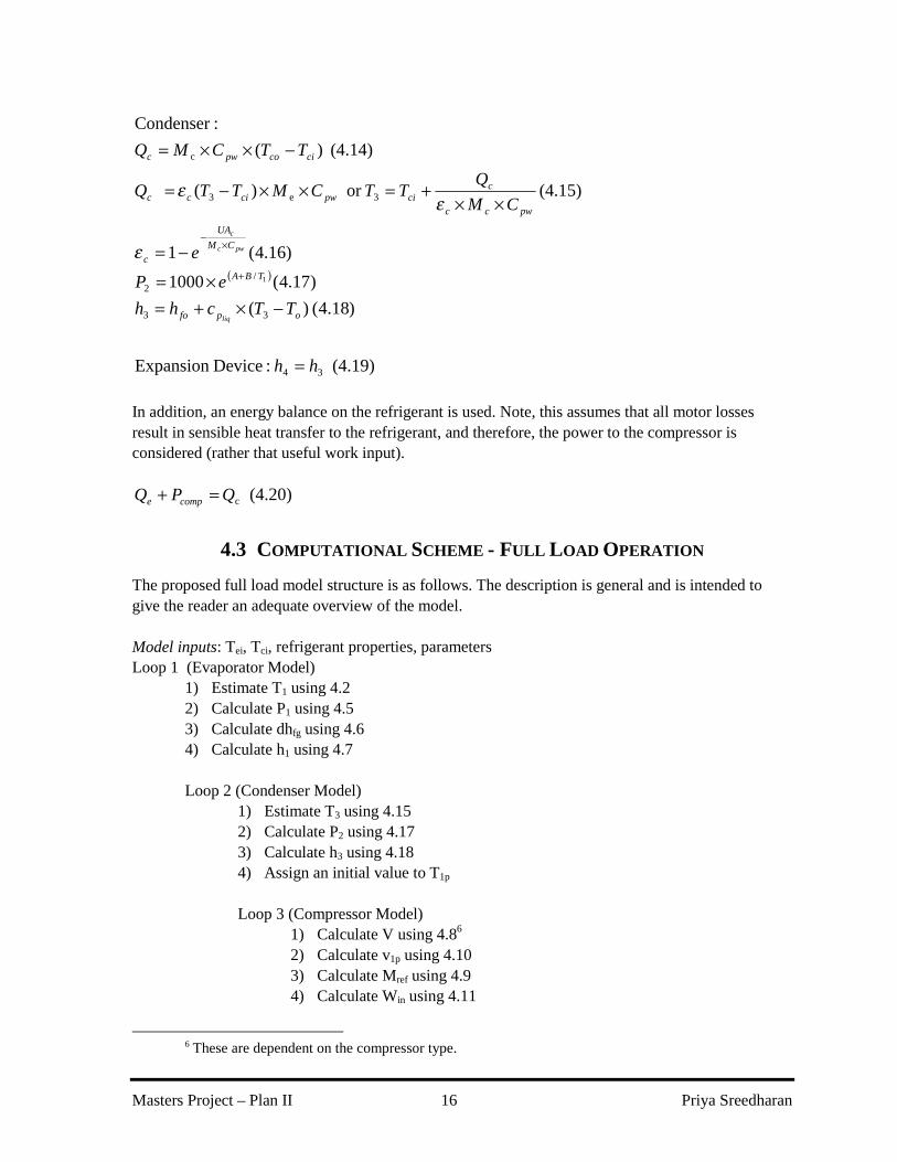
The proposed full load model structure is as follows. The description is general and is intended to give the reader an adequate overview of the model. Model inputs: Tei, Tci, refrigerant properties, parameters Loop 1 (Evaporator Model)
1) Estimate T1 using 4.2 2) Calculate P1 using 4.5 3) Calculate dhfg using 4.6 4) Calculate h1 using 4.7 Loop 2 (Condenser Model)
1) Estimate T3 using 4.15 2) Calculate P2 using 4.17 3) Calculate h3 using 4.18 4) Assign an initial value to T1p Loop 3 (Compressor Model)
1) Calculate V using 4.86 2) Calculate v1p using 4.10 3) Calculate Mref using 4.9 4) Calculate Win using 4.11
6 These are dependent on the compressor type.

Masters Project – Plan II 17 Priya Sreedharan
5) Calculate Pcomp using 4.12 6) Calculate T1p using 4.13 7) Exit Loop 3 when converged on T1p
End of Loop 3 5) Recalculate Qc using 4.20 6) Exit Loop 2 when converged on Qc
End of Loop 2 5) Recalculate Qe using 4.3 and 4.18 6) Exit Loop 1 when converged on Qe
End of Loop 3 Model Outputs: Teo, Tco (both calculated using 4.1 and 4.14 respectively), Pcomp
4.4 PART LOAD VARIATIONS
At full-load the chiller is cooling the evaporator water to the lowest possible temperature. The “chilled” water setpoint determines how hard the chiller must work in order to deliver the required cooling load. If the chiller does not have to work as hard to achieve a certain setpoint, then it is operated at part-load. At part-load, the refrigerant flow rate is reduced, which reduces the cooling capacity of the chiller. The refrigerant flow rate reduction is achieved in different ways: if the motor is variable speed, then a reduction in the rotational speed will result in a decrease in refrigerant flow rate. The other method is to change the volumetric displacement. For example, in reciprocating compressors, cylinders are unloaded. In centrifugal compressors, inlet guide vanes are partially closed to restrict flow. The Toolkit incorporates only the latter method, and not variable speed motors (although, this would not be a difficult to incorporate by the user). For reciprocating compressors, the number of unloaded cylinders is specified (or estimated), and closely resembles the actual part-load mechanism. In centrifugal compressors, however, the inlet guide vane restriction is modeled as a throttling process prior to compression. The throttling reduces the pressure of the refrigerant, thus, increasing the specific volume (decreasing the density). This, in turn combined with the ‘full-load’ volumetric displacement, that is specified by the compressor configuration results in a reduction in refrigerant mass flow rate.
4.5 CALIBRATION OF ORIGINAL TOOLKIT MODEL
The toolkit requires several parameters, including the heat exchanger coefficients (UAe and UAc), compressor loss parameters (Wlo, α), as well as the compressor specific parameters that determine the volumetric displacement.7 The toolkit contains a variety of parameterization routines, depending on the available data. In order parameterize a centrifugal chiller, the data required are: evaporator load, compressor power, inlet and
7 For centrifugal compressors, these other parameters are based on the “Velocity Triangle” of the impeller, which
includes the tangential velocity of impeller (U), and the absolute velocity of the fluid (C).

Masters Project – Plan II 18 Priya Sreedharan
exit water temperatures, and water flow rates, all at full load.8 The heat exchanger parameters (UA’s) are initially estimated by assuming a temperature difference of 5 K between the chilled water temperature and refrigerant (Teo-T1) and condenser outlet water temperature and refrigerant (T3-Tco). With the knowledge of the heat exchanger parameters, the effectiveness, and condensing and evaporating temperatures are calculated for each operating point. The refrigerant mass flow rate, and isentropic compression work to the compressor are directly calculated. Using this information, the compressor loss terms are estimated using linear regression. The remaining compressor parameters are calculated by a search method, such that the error between the estimated and measured compressor power is minimized. Finally, the heat exchanger parameters are recalculated at a fictitious operating point that is characterized by the average values of the evaporator load, condenser load, and water flow rates. (Bourdouxhe, 1994)
4.6 MODIFICATIONS TO THE MODEL AND COMPUTATIONAL SCHEME
The original Toolkit model’s purpose is to determine if a particular evaporator setpoint was achievable under specified operating conditions, and if so, by how much power. In addition, the calibration of the centrifugal chiller required full-load data. In contrast, the purpose of this paper was to compare the diagnostic capability of the Toolkit model. Particularly, at a given chiller evaporator load, could the compressor power consumption be accurately predicted. In addition, neither of the data sets obtained had significant number of full-load data. The modifications made to the original model, and computational scheme converted the Toolkit to the desirable form, that is not dependent on the control mode (i.e., full-load, part-load), nor on the compressor type, and can be calibrated with part-load data. The compressor loss relationship (4.12), which relates useful work input to compressor power is valid for all compressor types. The only equation presented in the full-load routine that is not universal to all compressor types is volumetric displacement (4.8). If the compressor power is known, and is used as an input to the model, then the refrigerant mass flow rate, and evaporator load can be calculated, using (4.12) and (4.11). The volumetric displacement relationship, therefore, is not required. One assumption was made with this restructuring: Recall, the part-load operation is modeled as a throttling process prior to compression. This pressure drop results in an increase in the specific volume of the refrigerant, which in turn achieved a reduced refrigerant flow rate. The reduced or "part-load" refrigerant flow rate was then used to compute work input to the compressor. Since the original model structure maintained both compressor power and evaporator load as 'outputs', this "throttling" was the only way to force part-load conditions (i.e., reduce refrigerant mass flow rate). However, with this restructuring, where compressor power is used as an input, and evaporator load is predicted (or vice versa, where evaporator load is the input, and compressor power is the output to match the other models). In computing refrigerant flow rate from useful compressor work, the specific volume of the refrigerant, in the absence of this part-load throttling process is used. This is appropriate since the throttle effect was primarily present to reduce mass flow rate, which is unnecessary in the modified structure where actual compressor power is known. The advantages that result from these modifications are listed:
8 The parameters are found using the full-load routine.
Masters Project – Plan II 19 Priya Sreedharan
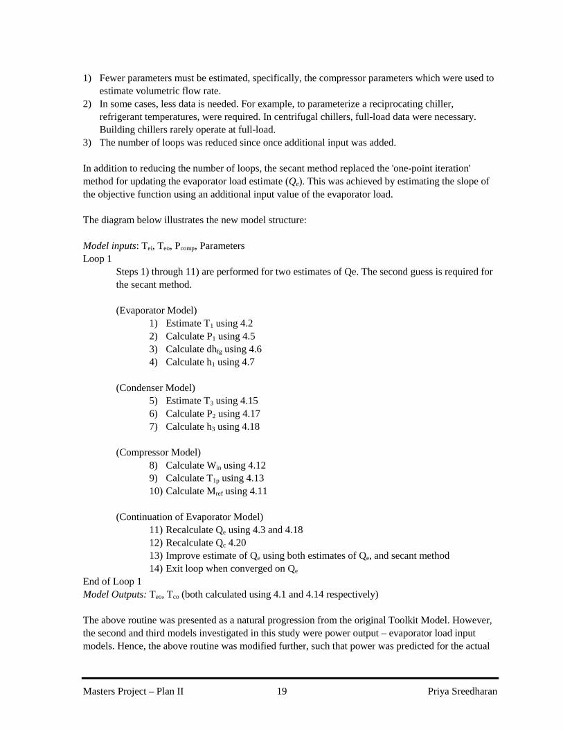
1) Fewer parameters must be estimated, specifically, the compressor parameters which were used to estimate volumetric flow rate.
2) In some cases, less data is needed. For example, to parameterize a reciprocating chiller, refrigerant temperatures, were required. In centrifugal chillers, full-load data were necessary. Building chillers rarely operate at full-load.
3) The number of loops was reduced since once additional input was added. In addition to reducing the number of loops, the secant method replaced the 'one-point iteration' method for updating the evaporator load estimate (Qe). This was achieved by estimating the slope of the objective function using an additional input value of the evaporator load. The diagram below illustrates the new model structure: Model inputs: Tei, Teo, Pcomp, Parameters Loop 1
Steps 1) through 11) are performed for two estimates of Qe. The second guess is required for the secant method. (Evaporator Model)
1) Estimate T1 using 4.2 2) Calculate P1 using 4.5 3) Calculate dhfg using 4.6 4) Calculate h1 using 4.7
(Condenser Model) 5) Estimate T3 using 4.15 6) Calculate P2 using 4.17 7) Calculate h3 using 4.18
(Compressor Model)
8) Calculate Win using 4.12 9) Calculate T1p using 4.13 10) Calculate Mref using 4.11
(Continuation of Evaporator Model) 11) Recalculate Qe using 4.3 and 4.18 12) Recalculate Qc 4.20 13) Improve estimate of Qe using both estimates of Qe, and secant method 14) Exit loop when converged on Qe
End of Loop 1 Model Outputs: Teo, Tco (both calculated using 4.1 and 4.14 respectively) The above routine was presented as a natural progression from the original Toolkit Model. However, the second and third models investigated in this study were power output – evaporator load input models. Hence, the above routine was modified further, such that power was predicted for the actual
Masters Project – Plan II 20 Priya Sreedharan
evaporator load. This was easily achieved by placing a larger loop around the entire routine, where for given evaporator load, power was predicted. The secant method was used here as well, to ensure quick convergence upon the compressor power (Pcomp) more efficiently. Note, the modified model still has fewer loops, and a more efficient routine (secant-method vs. one-point iteration) for convergence.
4.7 CALIBRATION OF MODIFIED TOOLKIT MODEL
The previous section described the modifications made to the original Toolkit model, as well as changes to the computational scheme. Four parameters were left to be estimated: the evaporator and condenser heat transfer coefficients, the compressor constant losses, and losses proportional to the power. Rather than adapting the parameter estimation schemes proposed in the reference, a different approach was used. The field of optimization has produced a variety of routines that can minimize a multi-variable function by simply using starting conditions, and the value of the function. These methods are called direct search methods, and are ideal for HVAC applications, where the equations are non-linear in the parameters. The following section very briefly introduces the subject of multi-variable optimization, describes the various direct search methods in limited detail, as well as the particular direct search method used to estimate the Toolkit parameters.
4.7.1 OPTIMIZATION INTRODUCTION
A function can be optimized using two broad methods: direct (numerical) or indirect (analytic). In direct methods, the solution is approached in an iterative manner, with each step hopefully improving the value of the objective function. Indirect methods attempt to reach the optimum in a single step without tests or trials, by analysis of the properties of the objective function; often this property is setting the partial derivative of the objective function with respect to each variable to zero. (Schwefel, 1995)
i allfor 0=∂∂
ix
f
The secant method that was used to improve the computational scheme of the Toolkit model is an example of an indirect method. That method is simple since the objective function is only a function of one variable. The Toolkit model is a complicated looped structure, whose equations cannot be reduced to a set of equations of known values that are linear in the parameters.9 Nor can the objective function, or error function, be written explicitly in terms of the known inputs and parameters. In fact, since the thermodynamic properties are a function of temperature and pressure, which themselves are estimated within the program, are not “known”. It is for these situations, where the partial derivatives of the function are not easily evaluated, that direct search methods are useful. They depend solely on the values of the objective function. The root mean square error was considered as the objective function:
9 This is true for this study, where part-load data is used to calibrate the model. Bourdouxhe (1994) did provide a
full-load calibration scheme that is a combination of linear regression and a grid-type search method.

Masters Project – Plan II 21 Priya Sreedharan
( )∑ −= 2 XmeasXpredRMSE
The value of X depends on which model prediction is desired, that is, whether power or evaporator load is the desired output. Since the remaining models discussed are based on power predictions, only that case will be discussed. A brief description of direct search methods in general is included, followed by a more detailed description of the particular direct search method employed.
4.7.2 DIRECT SEARCH METHODS
There are a variety of multidimensional direct search methods available. They can be compared using various criteria: computation efficiency (i.e., number of iterations required to find a solution), convergence success (i.e., whether a solution is reached), and type of minima found (i.e., global vs. local minima). To illustrate the need for an efficient direct search method, consider the “Equidistant Grid Strategy”. An evenly meshed grid is placed over the space of all possible parameter values and the objective function is evaluated at each node. This method is by far the most computationally expensive, and requires that the problem be constrained in the parameters. By “Bellman’s Curse of Dimensions”, the number of computations increases exponentially with the number of variables. All direct search strategies assume a degree of smoothness in the objective function. None converge with certainty to the global minimum; at best local minima are found. This is true, not only for direct search methods, but gradient (based on first order partial derivatives) and Newton (based on second order partial derivatives) methods. The solution is therefore, extremely sensitive to the initial conditions. They are attractive not for the theoretical proofs of convergence, but for the fact that they are simple and have worked in practice. The most well known direct search methods are: 1) Coordinate Strategy, 2) Hooke and Jeeves Pattern Search, 3) Rosenbrock Rotating Coordinates, 4) Davies, Swann, and Campey Method, 5) Box’s Complex Strategy Method, and 6) Nelder –Mead Simplex Method. All methods employ a trial and error approach. This means that while rules are used to vary the parameter, in the hope of a better objective function value, there is no guarantee of a successful step. These “rules” are what differentiate the various methods. Schwefel compared these methods on the basis of convergence efficiency and number of parameters. At this moment, there is no widely accepted function that can be used for such comparison purposes, hence, Schwefel used a few different function types for his comparison. Since a summary cannot properly describe this comparison, the reader is referred to the reference for the results of this comparison. However, since there is no accepted function for comparison purposes, there is no universal or ‘optimal’ optimization method. The Nelder-Mead and Hooke-Jeeves methods appear to be widely popular in the optimization community (Wetter, 2001). A proof of convergence has been presented for the Hooke-Jeeves algorithm, although neither method distinguishes between global or local minima. Due to its
Masters Project – Plan II 22 Priya Sreedharan
availability in the programming environment used in this study, the Nelder-Mead Simplex direct search method was chosen to find the parameter values that minimized the value of the objective function.
4.7.3 NELDER-MEAD SIMPLEX METHOD10
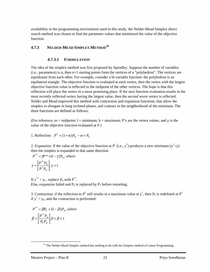
4.7.3.1 FORMULATION
The idea of the simplex method was first proposed by Spendley. Suppose the number of variables (i.e., parameters) is n, then n+1 starting points form the vertices of a “polyhedron”. The vertices are equidistant from each other. For example, consider a bi-variable function: the polyhedron is an equilateral triangle. The objective function is evaluated at each vertex, then the vertex with the largest objective function value is reflected in the midpoint of the other vertices. The hope is that this reflection will place the vertex in a more promising place. If the next function evaluation results in the most recently reflected vertex having the largest value, then the second worst vertex is reflected. Nelder and Mead improved this method with contraction and expansion functions, that allow the simplex to elongate in long inclined planes, and contract in the neighborhood of the minimum. The three functions are defined as follows: (For reference, m = midpoint; l = minimum; h = maximum; P’s are the vertex values, and y is the value of the objective function evaluated at P.)
1. Reflection: hm PPP ×−+= αα )(1 *
2. Expansion: If the value of the objective function at P* (i.e., y*) produces a new minimum (y*<y) then the simplex is expanded in that same direction
1,
,)1(*
*
**
**
>=
−+=
γγ
γγ
m
m
m
PP
PP
wherePPP
If y** < yl , replace Ph with P**. Else, expansion failed and Ph is replaced by P* before restarting. 3. Contraction: if the reflection to P* still results in a maximum value at y*, then Ph is redefined as P* if y* < yh, and the contraction is performed:
10,
,)1( **
**
<<=
−+=
ββ
ββ
mh
m
mh
PP
PP
wherePPP
10 The Nelder-Mead Simplex method has nothing to do with the Simplex method of Linear Programming.

Masters Project – Plan II 23 Priya Sreedharan
As long as y** < min (yh,y*), then P** replaces Ph. Otherwise, the contraction failed contraction, and all
vertices are replaced with the average between it’s value and the vertex with the minimum y value.
2 li
i
PPP
+=
4.7.3.2 OTHER ISSUES
If the variables are constrained, these constraints can be incorporated easily into the method by penalizing the objective function (i.e., setting it equal to a very large number) in disallowed values of the variables. Nelder and Mead compared the simplex method to the indirect, gradient based method of Powell. The convergence criterion was that the root mean square (r.m.s.) error should be less than 10-8. The N-M simplex method performed slightly better than Powell's method for two functions; convergence of the third function was strongly dependent on the initial step length, and was both more efficient and less efficient for different step lengths. For a number of variables between 2 and 10, the number of evaluations can be approximated by:
( ) 11.213.16 += kN
Consider a two variable problem, for which the variables are constrained between 1 and 100. (i.e., 1<x1, x2<100). Selecting an increment of 1 and using the equidistant grid strategy, the number of evaluations would be 100x100 = 10,000 evaluations. Using the above formula, the Nelder Mead method should take 32 function evaluations, which results in a reduction of evaluations by more than 99%. Not only, would the solution be converged upon more quickly, but two additional benefits are found: 1) the variables do not need to be constrained, and 2) the variables are not limited to specific intervals, as they are in the grid strategy. In summary, this method: 1) does not use derivatives, 2) requires little information of the function, and makes no assumptions about the surface, except
that it is continuous and has a unique minimum in the area of search (i.e., the algorithm cannot distinguish between a local minimum in the search area, and other minima outside the search area),
3) does well compared to gradient methods when curvature changes rapidly, and 4) may falsely converge in the case of a space having a long, curved valley, with extremely steep
sides.

Masters Project – Plan II 24 Priya Sreedharan
5. GORDON-NG UNIVERSAL CHILLER MODEL
5.1 INTRODUCTION
The Gordon –Ng model was first developed in 1994, and then refined later. (Gordon, 1995) The second generation model relies purely on the first and second laws of thermodynamics, heat transfer relationships, and makes simplifications where appropriate to derive an equation that relates COP to commonly measured parameters, including inlet evaporator and condenser temperatures, and evaporator load. The resulting equation can be rearranged to a form that is linear in the parameters, and can be calibrated using linear regression. (Ng, 1996, 1997)
5.2 DESCRIPTION AND CALIBRATION
The model begins with a first law energy balance on the refrigerant. This balance includes energy leaks at the evaporator, condenser and compressor:
positive are flowsenergy all where
(5.1) 0 ,, =+−−−+ leakcompcompeleakecleakc QPQQQQ
From the second law, an entropy balance is performed on the refrigerant:
g) throttlinand
n compressio isentropic-non (i.e., losses frictional todue generationentropy internal totalis S where
(5.2) 0
T
,
∆
=∆−+
−+
Tevap
eleake
cond
leak,cc ST
T
As in the ASHRAE Toolkit model, sensible heat exchange is ignored in both the condenser and the evaporator, which are modeled using the effectiveness-NTU method assuming an infinite capacity on the refrigerant side:
(5.4) )(),()()(
(5.3) )(),()()(
,,
,,
epweevaprefevapeievaprefevapeiepwee
cpwccondcirefcondcondcirefcondcpwcc
CMCTTCTTCMQ
CMCTTCTTCMQ
εεεε
≡−=−×=
≡−=−×=
The COP is defined as the ratio of evaporator load to power, and the equations are simplified by neglecting energy leaks and entropy generation in expressions where they are small compared to other terms. These approximations were based on experimental measurements. The simplification of the above equations results in the following chiller performance equation:

Masters Project – Plan II 25 Priya Sreedharan
( )
(5.5) 1
111
1 ,
+
×+
×−
+∆=−
+
COPT
QR
QT
TTQS
Q
T
COPT
T
ci
e
eci
eicieqvleakT
e
ei
ci
ie
The three performance parameters are: a) total internal entropy production, ∆ST b) total heat exchanger 'thermal resistance'11,
pweepwcc CMCMR
εε11
+=(5.6)
c) equivalent heat leak,
eici
eicompleakeleakeqvleak TT
TQQQ
−×
+= ,,,
Although Qleak,eqv has a dependence on temperatures, the authors claim this dependence exerts a small influence on COP for properly operating commercial chillers. While the other parameters may also have slight dependence on temperatures, the authors found that adopting constant values resulted in performance predictions whose errors are less than the effects of typical measurement errors. The model is calibrated by fitting the function on the left side to the variables x1, x2, and x3, which are defined as,
( )
+=
×−
==COPT
Qx
QT
TTx
Q
Tx
ci
e
eci
ieci
e
ei 113 ,2 ,1
Once calibrated, the equation is rearranged to solve for COP, or Power explicitly.
5.3 COMPARISON BETWEEN TOOLKIT AND GORDON-NG MODELS
Both the Toolkit and Gordon-Ng models are based on first principles, but are different their assumptions, and approach. These are listed in Table 5.1.
11 Note that R is not equal to the sum of the reciprocals of the conventional UA values, but of UA values defined
in terms of the difference between the inlet water temperature and the refrigerant temperature, rather than the log mean temperature difference.
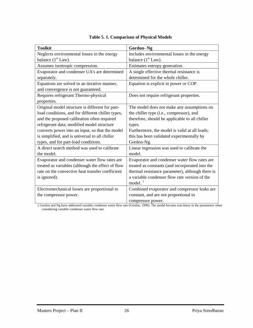
Masters Project – Plan II 26 Priya Sreedharan
Table 5. 1. Comparison of Physical Models
Toolkit Gordon- Ng Neglects environmental losses in the energy balance (1st Law).
Includes environmental losses in the energy balance (1st Law).
Assumes isentropic compression. Estimates entropy generation. Evaporator and condenser UA's are determined separately.
A single effective thermal resistance is determined for the whole chiller.
Equations are solved in an iterative manner, and convergence is not guaranteed.
Equation is explicit in power or COP.
Requires refrigerant Thermo-physical properties.
Does not require refrigerant properties.
Original model structure is different for part-load conditions, and for different chiller types, and the proposed calibration often required refrigerant data; modified model structure converts power into an input, so that the model is simplified, and is universal to all chiller types, and for part-load conditions.
The model does not make any assumptions on the chiller type (i.e., compressor), and therefore, should be applicable to all chiller types. Furthermore, the model is valid at all loads; this has been validated experimentally by Gordon-Ng.
A direct search method was used to calibrate the model.
Linear regression was used to calibrate the model.
Evaporator and condenser water flow rates are treated as variables (although the effect of flow rate on the convective heat transfer coefficient is ignored).
Evaporator and condenser water flow rates are treated as constants (and incorporated into the thermal resistance parameter), although there is a variable condenser flow rate version of the model. 1
Electromechanical losses are proportional to the compressor power.
Combined evaporator and compressor leaks are constant, and are not proportional to compressor power.
1 Gordon and Ng have addressed variable condenser water flow rate (Gordon, 1999). The model became non-linear in the parameters when considering variable condenser water flow rate.

Masters Project – Plan II 27 Priya Sreedharan
6. EMPIRICAL MODEL (DOE-2/COOLTOOLS)
6.1 INTRODUCTION
The DOE-2 model was developed by the Department of Energy as a tool to help guide architects, and engineers to design more energy efficient buildings. Within the DOE-2 program is a chiller module that simulates chiller performance. The DOE-2 chiller model (hereafter referred to as DOE-2 model) is based on three polynomial curves. They describe how the cooling capacity and efficiency (kW/ton) vary with operating conditions, as well as how the power consumption varies at part load conditions. They are empirical in the sense that the polynomial structure is not based on physical relationships. However, the model is somewhat a grey-box model, since the final power prediction of the chiller is based on physically meaningful quantities obtained from the polynomial curves. An assumption the model makes is that evaporator and condenser water flow rates remain constant. (PG&E, 1999)
6.2 DESCRIPTION
The three curves in DOE-2 are defined as follows:
(6.3) ,
,
(6.2)
(6.1)
),(
2333
22
222
222
12
112
111
TciTeoavailablee
e
cieicicieoeo
cieocicieoeo
Q
QPLRwherePLRcPLRbaEIRFPLR
TTfTeTdTcTbaEIRFT
TTfTeTdTcTbaCAPFT
=×+×+=
××+×+×+×+×+=
××+×+×+×+×+=
The first curve describes how the cooling capacity of the chiller varies at different evaporator and condenser water temperatures, in comparison to the cooling capacity at reference conditions. The reference conditions can be any temperature, so long as they are consistent. According to ARI standards, these reference temperatures are 44 °F (6.7 °C ) and 85 °F (29.4 °C). Q ref, and P ref are the full load cooling capacity, and power consumption at the reference chilled and condenser water temperatures. Thus,
(6.4) ,
,
refe
availablee
Q
QCAPFT =
The second curve describes how the full load (in)efficiency, defined as power consumption in kW per ton of cooling varies with water temperatures. This is also a dimensionless term where,
(6.5) max
,
, ref
refe
availablee P
Q
Q
PEIRFT ×=
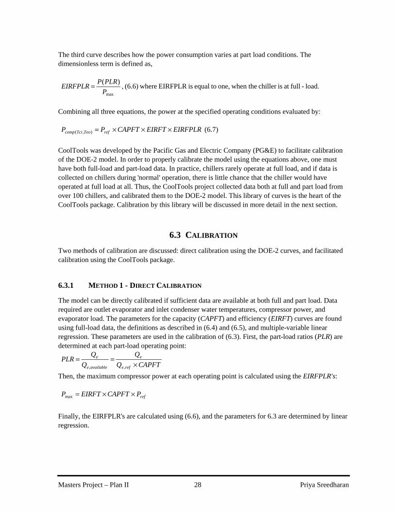
Masters Project – Plan II 28 Priya Sreedharan
The third curve describes how the power consumption varies at part load conditions. The dimensionless term is defined as,
load.-fullat ischiller when theone, toequal is EIRFPLR where(6.6) , )(
maxP
PLRPEIRFPLR =
Combining all three equations, the power at the specified operating conditions evaluated by:
(6.7) ),( EIRFPLREIRFTCAPFTPP refTeoTcicomp ×××=
CoolTools was developed by the Pacific Gas and Electric Company (PG&E) to facilitate calibration of the DOE-2 model. In order to properly calibrate the model using the equations above, one must have both full-load and part-load data. In practice, chillers rarely operate at full load, and if data is collected on chillers during 'normal' operation, there is little chance that the chiller would have operated at full load at all. Thus, the CoolTools project collected data both at full and part load from over 100 chillers, and calibrated them to the DOE-2 model. This library of curves is the heart of the CoolTools package. Calibration by this library will be discussed in more detail in the next section.
6.3 CALIBRATION
Two methods of calibration are discussed: direct calibration using the DOE-2 curves, and facilitated calibration using the CoolTools package.
6.3.1 METHOD 1 - DIRECT CALIBRATION
The model can be directly calibrated if sufficient data are available at both full and part load. Data required are outlet evaporator and inlet condenser water temperatures, compressor power, and evaporator load. The parameters for the capacity (CAPFT) and efficiency (EIRFT) curves are found using full-load data, the definitions as described in (6.4) and (6.5), and multiple-variable linear regression. These parameters are used in the calibration of (6.3). First, the part-load ratios (PLR) are determined at each part-load operating point:
CAPFTQ
Q
Q
QPLR
refe
e
availablee
e
×==
,,
Then, the maximum compressor power at each operating point is calculated using the EIRFPLR's:
refPCAPFTEIRFTP ××=max
Finally, the EIRFPLR's are calculated using (6.6), and the parameters for 6.3 are determined by linear regression.

Masters Project – Plan II 29 Priya Sreedharan
6.3.2 METHOD 2 - CALIBRATION BY THE COOLTOOLS LIBRARY OF CURVES
The second method involves using the CoolTools automated calibration procedure. To facilitate the calibration of the DOE-2 chiller model from field operating data, the CoolTools project collected operating data both at full and part load from over 100 chillers and used these data to generate a library of curves that is included in the CoolTools package. When limited performance data are available, a curve that matches the data can be selected from the library, resulting in a significantly better model than would have been obtainable otherwise.

Masters Project – Plan II 30 Priya Sreedharan
7. MEASURED DATA AND DATA PROCESSING
7.1 LABORATORY CHILLER
7.1.1 EXPERIMENTAL ARRANGEMENT
Performance data were collected from a centrifugal, 90 ton (316 kW) water-cooled McQuay chiller, with R-134 as the working fluid .12 The test stand was designed to meet the American Refrigeration Institute (ARI) specifications for testing chillers, with the goal of simulating the load of a real building. The chiller itself follows the basic design of most vapor-compression chillers (compressor – condenser – expansion valve – evaporator). The capacity of the chiller is controlled by adjusting the inlet guide vanes to the impeller of the compressor. The onboard chiller controller hydraulically regulates the vane position to achieve the desired setpoint temperature, although, the vane position is not monitored. The motor itself is external to the chiller, with a drive shaft connecting the motor to the compressor (compared to a hermetically sealed motor). A variation to the main refrigerant line, includes a separate motor cooling line which diverts refrigerant flow from the expansion valve to the motor, and recombines with the remaining refrigerant flow prior to entering the evaporator.
7.1.2 TEST SEQUENCE
ARI standards determine the range of condenser inlet temperatures, and evaporator outlet temperatures at which the chiller should be tested. In addition, the chiller was tested at various part-load conditions. The temperature guidelines were followed as closely as possible, but were limited in some cases. The most severe limitation was on the upper limit of the condenser temperatures, since larger condenser temperatures could result in surge (when the larger pressure lift causes the refrigerant to flow in the reverse direction). A matrix of test conditions was devised, such that the evaporator setpoint was changed as minimally as possible (in order to reach steady-state conditions more quickly). Chiller data at 27 different operating conditions were obtained.
7.1.3 MEASURED DATA AND SENSOR ACCURACY
Water flow rates and temperatures were measured on both the condenser and evaporator sides. Water temperatures at other locations were measured as well, but not used for chiller modeling. Temperatures were measured by two sensor types, thermistors, and Resistance Temperature Detectors (RTDs). (Two types of sensors were present, since one was part of the chiller control panel, and the other, the overall test stand controller.) The RTD measurements were reported as their accuracy was superior to the thermistors’. Vortex flow meters were used to measure the water flow rates. Compressor power was measured as well, by a watt transducer. Table 7.1 lists the sensors and their accuracy.
12 This data was collected by Purdue University, and was presented in the Report # 4036-3, available from the Ray
Herrick Laboratory, Purdue.

Masters Project – Plan II 31 Priya Sreedharan
Table 7.1: Sensors and Uncertainty
Point Sensor Type Uncertainty (%)
Uncertainty (Absolute Terms)
Water Temperatures Resistance Temperature Detector (RTD)
-- ± 0.05 F (0.03 C)
Evaporator Volumetric Flow Rate
Vortex Flow Meter (VFM) ±1 ± 2.2 gpm 1
(8.3 l/min) Evaporator Mass Flow Rate -- -- ± 0.14 kg/s 2
Condenser Volumetric Flow Rate
VFM ±1 ± 2.8 gpm 1
(10.6 l/min) Condenser Mass Flow Rate -- -- ± 0.18 kg/s 2
Compressor Power Watt Transducer ±1.5 ±1.3 kW 3
1 Calculated from the % uncertainty and design flow rates.
2 Calculated from the % uncertainty and assuming water density of 1 kg/l
3 Calculated from a full load power of 85 kW.
The data provided in the report had been filtered to remove the transient data, and were ready for analysis. However, prior to applying the data to the models, a simple energy balance was performed on the chiller to ensure that environmental losses were below acceptable standards. This step was considered important, since the ultimate objective of the model is to predict power measurements within high accuracy, and this cannot be achieved unless the data is considered to be accurate. The energy balance on the chiller is: Energy Balance = Qe + Pcomp – Qc (kW), where a positive energy balance implies energy loss at the compressor or condenser, and a negative energy balance implies energy gain at the evaporator.
7.2 FIELD (BUILDING) CHILLER
7.2.1 CHILLER AND BUILDING DESCRIPTION
Data was collected from an older 225 ton (791 kW) Carrier water-cooled centrifugal chiller, which uses R-11, over a period of 18 months.13 The chiller capacity was controlled by adjusting the inlet guide vanes of the compressor. Chiller data, along with other HVAC&R system data was collected as part of a building diagnostics project by Lawrence Berkeley National Laboratory (LBNL). Evaporator and condenser flow rates, temperatures, and compressor power were collected every minute using high quality sensors. (Piette, 1998)
13 The chiller was installed around 1970.

Masters Project – Plan II 32 Priya Sreedharan
7.2.2 SENSOR ACCURACY
Water temperatures were measured by precise thermistors, designed to eliminate sensor drift. The thermistors were calibrated to an accuracy of 0.008 °F (0.0044 °C) over a full range of values, using a NIST traceable procedure. Water flow rates were measured by magnetic flow meters, which were installed in sufficiently long sections of the pipe (as pipe bends affect accuracy). Power was measured by three phase power transducers. Table 7.2 lists the sensors with their accuracy.
Table 7.2: Sensors and Uncertainty
Point Sensor Type Uncertainty (%)
Uncertainty (Absolute Terms)
Water Temperatures Thermistors -- ± 0.008 °F (0.0044 °C)
Evaporator Volumetric Flow Rate
Magnetic Flow Meter (MFM)
±0.5 ± 2.9 gpm 1
(10.9 l/min) Evaporator Mass Flow Rate -- -- ± 0.18 kg/s 2
Condenser Volumetric Flow Rate
MFM ±0.5 ± 2.7 gpm 3
(10.1 l/min) Condenser Mass Flow Rate -- -- ± 0.17 kg/s 2
Compressor Power Watt Transducer ±0.2 ±0.36 kW 4
1 Calculated from the % uncertainty and an average flow rate of 577 gpm.
2 Calculated from the % uncertainty and assuming water density of 1 kg/l.
3 Calculated from the % uncertainty and an average flow rate of 534 gpm.
4 Calculated from full load power of 180 kW.
7.2.3 STEADY-STATE FILTERING AND DATA BINNING
A simple steady-state filter was developed to remove data from transient operation. In the chiller, transient behavior occurs during start-up and shut-down, as well as when the chilled water setpoint is changed, and is detectable by either unusually high or low efficiencies. A geometrically weighted average of the functional variation is calculated as follows:
A large forgetting factor favors the most recent data, while a small forgetting factor tightens the steady-state requirement. Both the forgetting factor and the threshold were tuned until the data appeared to be filtered thoroughly. The data was filtered by three data points: chilled water temperature, evaporator load, and condenser water temperature. (Piette, 1999)
threshold theis and factor, forgetting a is k, at time signal theof value theis where,
statesteady in is signal then , if
)1( 11
ty
tV
VyyV
k
k
kkkk
α
αα
<
−+−= −−

Masters Project – Plan II 33 Priya Sreedharan
In order to produce a representative data set for calibration of the models, the entire filtered data set was binned by chilled water temperature, condenser temperature, and evaporator load. The data in each bin were averaged, and these average values comprised the training data.

Masters Project – Plan II 34 Priya Sreedharan
8. UNCERTAINTY ANALYSIS
8.1 EVAPORATOR AND CONDENSER LOAD UNCERTAINTIES
Measurement error is comprised of two components: bias and precision errors. The bias consistently shifts the sampled mean from the true mean by a fixed amount. The precision, however, is scattered, and is normally distributed about the sampled mean. The combination of these independent errors results in the true error. This true error is what is known as uncertainty. Typically, the uncertainty guarantees that the measured value is within x% of the true value, with a confidence of 95%. The uncertainty in the individual measurements results in the propagation of error. In general, the uncertainty of a function is dependent on the uncertainties of each independent variable, and the sensitivity of the function to each variable. By approximating the uncertainty contributions from each variable with the first two terms of the Taylor series expansion, the uncertainty of a function, f, with variables, xi, is: (Figliola, 1995)
∑
×
∂∂±=
2
ixi
f ux
fu (8.1)
The calculated evaporator and condenser loads demonstrate error propagation, since each are dependent on three measured variables. (The specific heat of water, and densities are assumed constant.)
condenser and ,evaporator theacross sdifference re temperatupositive are T ,T
where,
(8.3) ,
(8.2) , Recall,
ce
cc
e
∆∆
∆××=
∆××=
cp
epe
TCMQ
TCMQ
The evaporator load uncertainty can be calculated using (8.1), and (8.2):
( ) ( )2222
)( MeepTepeMee
eTe
e
eQe uTCuCMu
M
Qu
T
QkWu ×∆×+××±=
×
∂∂
+
×
∆∂∂
±= ∆∆
It is often more convenient to represent the uncertainty in terms of a percentage. Dividing both sides by the evaporator load and multiplying by 100 results in:

Masters Project – Plan II 35 Priya Sreedharan
22
100 (%)
+
∆
×±= ∆
e
Me
e
TeQe M
u
T
uu
(8.4)
(8.4) requires the uncertainty of the temperature change, which is shown below:
( ) ( ) ( ) uniform) all weresensors atureour temper since ,( (8.5) 2 22eoeiTeiTeoTeiTe UTUTUUUu =±=+±=∆
The uncertainty of the condenser load can be calculated in a similar way, and is exactly analogous to (8.4):
22
100 (%)
+
∆
×±= ∆
c
Mc
c
TcQc M
u
T
uu
(8.6)
( ) ( ) ( ) (8.7) 2 22TciTcoTciTc UUUu =+±=∆
8.2 UNCERTAINTY IN MODELED PREDICTIONS
The uncertainty in the actual evaporator and condenser loads is easily calculated at each operating point using the above equations. However, the purpose of this study is to compare various chiller models, and identify those that are adequate for fault detection. In operation, the model would be used to determine when a fault is generated, that is, the error between the predicted power (for example), and actual power is above a predefined threshold. It is imperative to be able to differentiate between a true fault, and an error due to experimental uncertainty. Thus, the uncertainty of the model predictions due to error in the measured variables was investigated. When it is undesirable to calculate the sensitivities analytically (i.e., using partial derivatives), a finite difference approximation can be used. For example, if one variable is perturbed, the difference between the unperturbed function value and perturbed function value divided by the perturbation is the sensitivity to that variable. To evaluate the overall uncertainty in the function, the Sequential Perturbation method was used. (Figliola, 1995)
8.2.1 SEQUENTIAL PERTURBATION
The sequential perturbation method basically calculates the uncertainty in a worst case scenario. Each variable is perturbed one at a time to its maximum values, and then to its minimum values. The uncertainty due to each variable is based on the average, and the total uncertainty due to all variables is based on the sum of the squares of the uncertainties. Steps 1 through 6 describe this method:

Masters Project – Plan II 36 Priya Sreedharan
( )
±=
+=
−=−=
=
∑=
−+
−−++
−
+
2
1
.6
2 .5
and , 4.
etc. theseCall R. erecalculat and ies,uncertaint respectiveby their t variableindependeneach Decrease 3.
etc. theseCall R. erecalculat and ies,uncertaint respectiveby their t variableindependeneach Increase .2
st variableindependen dunperturbe .arex2,...xL.. x1, where)...,3,2,1( alc .1
L
iRiR
Ri
RiRi
u
RiRi
RoRiRoRi
Ri
Ri
xLxxxfRoC
δ
δ
δδ
Each variable requires 2 model runs, therefore, a total of 2L model runs is required to calculate the uncertainty in the model predictions.

Masters Project – Plan II 37 Priya Sreedharan
9. RESULTS – LABORATORY CASE STUDY
Section 9 presents the analysis of the data obtained from the laboratory chiller. Details of the chiller and experimental measurements were given in Section 7.1.
9.1 ENERGY BALANCE AND UNCERTAINTY IN LOAD CALCULATIONS
Figure 9.1 shows the energy balance as a function of the test (each test represented different operating conditions). The error bars represent the uncertainty range of the energy balance, following procedures described in Section 8, and 9.1.
( ) ( ) ( ) (9.1) )( 222QcPcompQenceEnergyBala UUUkWU ++±=
0.00
10.00
20.00
30.00
40.00
50.00
60.00
70.00
80.00
0 5 10 15 20 25 30Test
Ene
rgy
Bal
ance
(kW
)
Figure 9.1. Energy Balance
The maximum compressor power is 85 kW and evaporator load is 316 kW. The energy balance as a percentage of the maximum compressor power, and evaporator load, respectively, was calculated, and is shown in Figures 9.2 and 9.3.

Masters Project – Plan II 38 Priya Sreedharan
0%
10%
20%
30%
40%
50%
60%
70%
80%
90%
100%
0 5 10 15 20 25 30
Test
% o
f Ma
xim
um
Po
we
r
`
Figure 9.2. Energy Balance as Percentage of Maximum Power
0%
10%
20%
30%
40%
50%
60%
70%
80%
90%
100%
0 5 10 15 20 25 30
Test
% o
f Ma
xim
um E
vap
ora
tor L
oa
d
`
Figure 9.3. Energy Balance as Percentage of Maximum Evaporator Load
The uncertainty analysis confirmed that the observed energy imbalance is not due to sensor uncertainty alone. The energy imbalance was correlated with the evaporator load, condenser load, and compressor power. These results are shown in Figures 9.4 – 9.6.
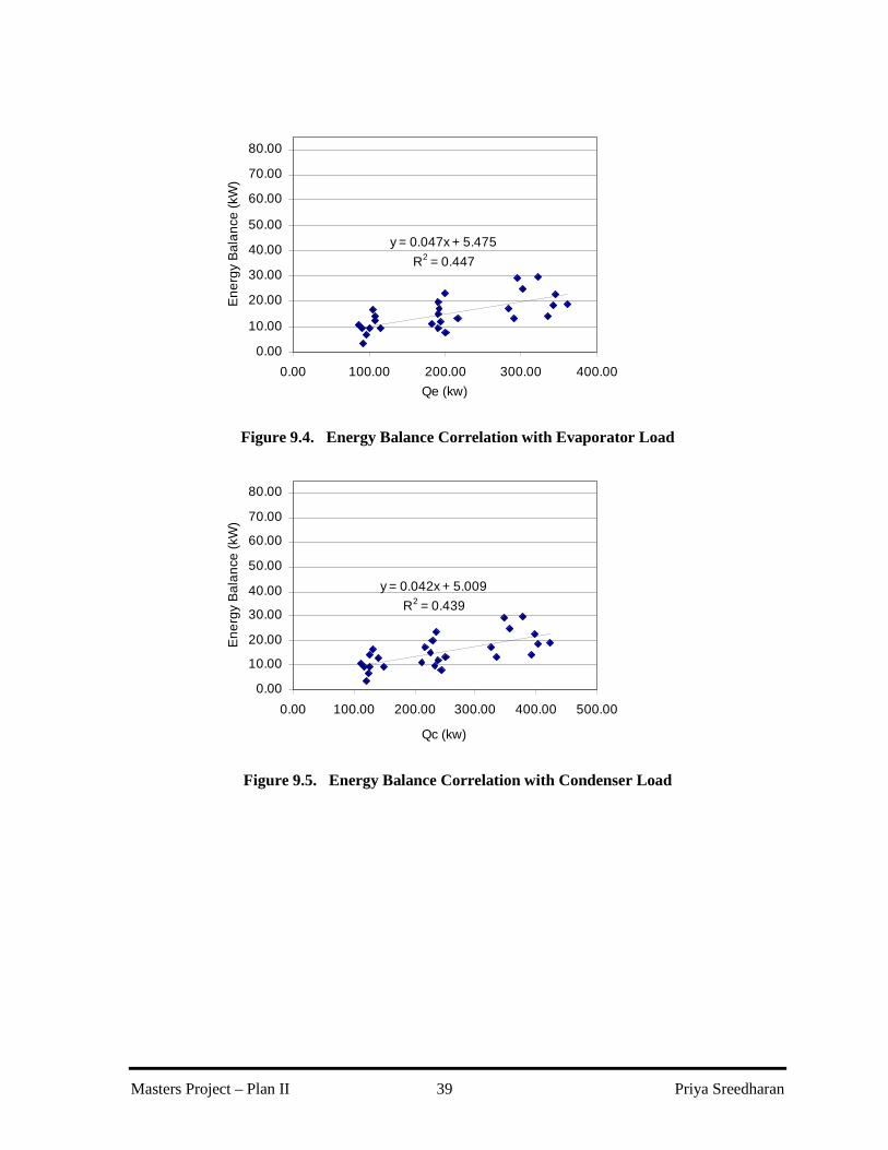
Masters Project – Plan II 39 Priya Sreedharan
y = 0.047x + 5.475
R2 = 0.447
0.00
10.00
20.00
30.00
40.00
50.00
60.00
70.00
80.00
0.00 100.00 200.00 300.00 400.00
Qe (kw)
En
erg
y B
ala
nce
(kW
)
Figure 9.4. Energy Balance Correlation with Evaporator Load
y = 0.042x + 5.009
R2 = 0.439
0.00
10.00
20.00
30.00
40.00
50.00
60.00
70.00
80.00
0.00 100.00 200.00 300.00 400.00 500.00
Qc (kw)
En
erg
y B
ala
nce
(kW
)
Figure 9.5. Energy Balance Correlation with Condenser Load

Masters Project – Plan II 40 Priya Sreedharan
y = 0.308x - 1.502
R2 = 0.637
0.00
10.00
20.00
30.00
40.00
50.00
60.00
70.00
80.00
0.00 20.00 40.00 60.00 80.00 100.00
P (kw)
En
erg
y B
ala
nce
(kW
)
Figure 9.6. Energy Balance Correlation with Compressor Power
The energy balance shows a significantly stronger correlation with the compressor power than with either the evaporator or condenser load. This suggests that the energy imbalance could be a result of electromechanical losses from the motor to the environment. Two versions of the laboratory data set were used to test the models, the original and one in which the compressor measurements were reduced by 30%, resulting in an approximately zero energy balance. Both data sets were used in order to observe the effect of the energy losses on the model predictions. The data set for which the power measurements were reduced are hereafter named “Adjusted Data”, and the unchanged data set are named "Original Data". Figures 9.7 and 9.8 shows the energy balance as a percentage of the maximum compressor power, and evaporator load after the power measurement adjustment.
-20%
0%
20%
40%
60%
80%
100%
0 5 10 15 20 25 30
Test
% o
f Ma
xim
um
Po
we
r
`

Masters Project – Plan II 41 Priya Sreedharan
Figure 9.7 Energy Balance (% Maximum Power)
-20%
0%
20%
40%
60%
80%
100%
0 5 10 15 20 25 30
Test
% o
f Ma
xim
um
Eva
po
rato
r Lo
ad
`
Figure 9.8 Energy Balance (% Maximum Evaporator Load)
The energy balance with adjusted power is within 10% of the maximum compressor power, and 2% of the maximum evaporator load. Figure 9.8 shows the adjusted energy balance with adjusted uncertainty analyses, as a function of test.
-15.00
-5.00
5.00
15.00
25.00
35.00
45.00
55.00
0 5 10 15 20 25 30
Test
Ene
rgy
Bal
ance
(kW
)
Figure 9.9 Adjusted Energy Balance
As seen in Figure 9.9, the adjusted energy balance, when accounted for uncertainty is approximately zero.
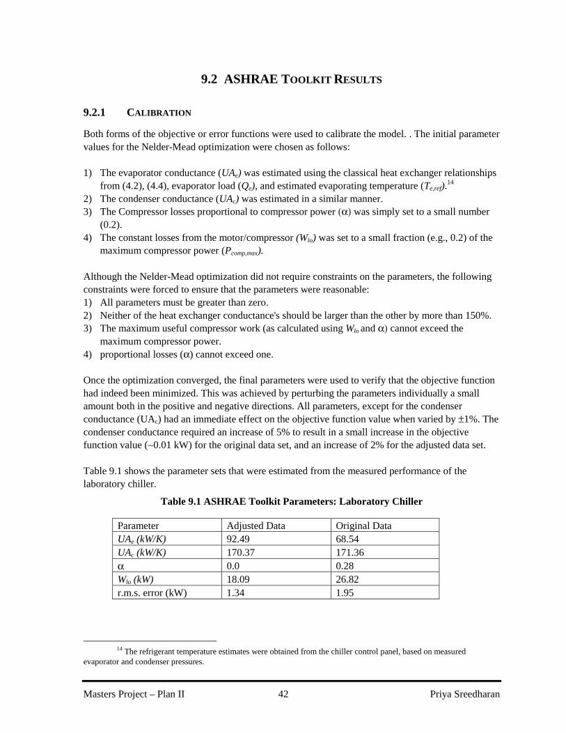
Masters Project – Plan II 42 Priya Sreedharan
9.2 ASHRAE TOOLKIT RESULTS
9.2.1 CALIBRATION
Both forms of the objective or error functions were used to calibrate the model. . The initial parameter values for the Nelder-Mead optimization were chosen as follows: 1) The evaporator conductance (UAe) was estimated using the classical heat exchanger relationships
from (4.2), (4.4), evaporator load (Qe), and estimated evaporating temperature (Te,ref).14
2) The condenser conductance (UAc) was estimated in a similar manner. 3) The Compressor losses proportional to compressor power (α) was simply set to a small number
(0.2). 4) The constant losses from the motor/compressor (Wlo) was set to a small fraction (e.g., 0.2) of the
maximum compressor power (Pcomp,max). Although the Nelder-Mead optimization did not require constraints on the parameters, the following constraints were forced to ensure that the parameters were reasonable: 1) All parameters must be greater than zero. 2) Neither of the heat exchanger conductance's should be larger than the other by more than 150%. 3) The maximum useful compressor work (as calculated using Wlo and α) cannot exceed the
maximum compressor power. 4) proportional losses (α) cannot exceed one. Once the optimization converged, the final parameters were used to verify that the objective function had indeed been minimized. This was achieved by perturbing the parameters individually a small amount both in the positive and negative directions. All parameters, except for the condenser conductance (UAc) had an immediate effect on the objective function value when varied by ±1%. The condenser conductance required an increase of 5% to result in a small increase in the objective function value (∼0.01 kW) for the original data set, and an increase of 2% for the adjusted data set. Table 9.1 shows the parameter sets that were estimated from the measured performance of the laboratory chiller.
Table 9.1 ASHRAE Toolkit Parameters: Laboratory Chiller
Parameter Adjusted Data Original Data UAe (kW/K) 92.49 68.54 UAc (kW/K) 170.37 171.36 α 0.0 0.28 Wlo (kW) 18.09 26.82 r.m.s. error (kW) 1.34 1.95
14 The refrigerant temperature estimates were obtained from the chiller control panel, based on measured
evaporator and condenser pressures.

Masters Project – Plan II 43 Priya Sreedharan
In addition to verifying that a true minimum was found, the model was exercised with a range of parameter values for both heat exchanger conductances (UAe and UAc), maintaining the other parameters (Wlo and α) at their optimized values to observe the shape of the objective function and verify that a global minimum, rather than an isolated local minimum was found. The surface graphs from this exercise are presented in figures 9.10 and 9.11.
Figure 9.10. ASHRAE Toolkit Results - Laboratory Chiller - Objective Function (Adjusted
Data)

Masters Project – Plan II 44 Priya Sreedharan
Figure 9.11. ASHRAE Toolkit Results - Laboratory Chiller - Objective Function (Original
Data)
Overall, the shapes of both surfaces were quite similar, which follows the expected behavior, in that the heat exchanger UA's are inversely related. The sum of the reciprocals of the UA's is approximately constant, indicating that the total thermal resistance of the condenser and the evaporator is well-defined by the performance data.
9.2.2 MODEL RESULTS
Comparisons of the predicted and measured compressor powers are shown in figures 9.12 and 9.13.

Masters Project – Plan II 45 Priya Sreedharan
0
10
20
30
40
50
60
70
0 10 20 30 40 50 60 70Measured Pow er (kw )
Pre
dict
ed P
ower
(kw
)
Figure 9.12. ASHRAE Toolkit Results - Laboratory Chiller (Adjusted Data)
0
10
20
30
40
50
60
70
80
90
0 10 20 30 40 50 60 70 80 90
Measured Power (kw)
Pre
dict
ed
Pow
er (
kw)
Figure 9.13. ASHRAE Toolkit Results - Laboratory Chiller (Original Data)
Table 9.2 presents the statistical analysis for the model predictions.

Masters Project – Plan II 46 Priya Sreedharan
Table 9.2. Statistical Analysis of Toolkit Model Results
Statistical Value Adjusted Data Original Data Average Error (kW) 1.11 1.56 Error (%) 3.02 2.98 r.m.s. error (kW) 1.34 1.95 r.m.s. error (%) 3.54 3.69
Since the condenser and evaporator pressures were available, the internally predicted pressures for both the heat exchangers are shown in figures 9.14 and 9.15. (The results from the original data set are shown, since the results from the adjusted data set were similar.)
0
50
100
150
200
250
300
350
400
450
0 50 100 150 200 250 300 350 400 450
Measured (kPa)
Pre
dic
ted
(kP
a)
Figure 9.14. Evaporator Pressure Model Predictions (Original Data)

Masters Project – Plan II 47 Priya Sreedharan
0
100
200
300
400
500
600
700
800
900
1000
0 100 200 300 400 500 600 700 800 900 1000
Measured (kPa)
Pre
dic
ted
(kP
a)
Figure 9.15. Condenser Pressure Model Predictions (Original Data)
The evaporating pressures are overestimated, particularly at higher pressures, while the condensing pressures are slightly underestimated. Condensing and evaporating pressures correlate directly with the evaporating and condensing temperatures. This implies that, based on the heat transfer, and heat exchanger effectiveness relationships, both the evaporator and condenser conductance’s are overestimated. This result was expected, since, in both cases, the sensible heat transfer was not considered separately, and was lumped into the isothermal heat transfer process. A sequential perturbation analysis was performed to determine the uncertainty in the power predictions. Figure 9.16 shows the results from this analysis. This analysis was performed using the original data set.

Masters Project – Plan II 48 Priya Sreedharan
0
10
20
30
40
50
60
70
80
90
0 10 20 30 40 50 60 70 80 90
Measured Pow er (kw )
Pre
dict
ed P
ower
(kw
)
Figure 9.16. ASHRAE Toolkit Results - Laboratory Chiller With Uncertainty Error Bars
(Original Data)
The r.m.s. error (kW) and r.m.s. error (%) of the uncertainty was calculated from the uncertainty at each individual operating point using the following function:
( )
points operatingnumber n where,)((%)
points operatingnumber n where,)(
2
1 ,
2
1
=
±=
=
±=
∑
∑
=
=
n
P
U
uRMSE
n
U
uRMSE
n
i dunperturbepred
Pi
P
n
iPi
P
Using the above formulae, the uncertainty in model predictions due to measurement errors in the input data is estimated to be 0.83 kW, or 1.37%. The Toolkit model assumes an energy balance in order to estimate the condenser load. Therefore, the energy losses from the compressor resulted in an overestimation of the condenser load when the original data was used. In the case of the adjusted data, the condenser load was more accurately predicted. Figure 9.17 shows the condenser load predictions for both cases.

Masters Project – Plan II 49 Priya Sreedharan
0
50
100
150
200
250
300
350
400
450
500
0 50 100 150 200 250 300 350 400 450 500
Measured Condenser Load (kW)
Pre
dic
ted
Co
nde
nse
r L
oad
(kW
)
"Original Data"
"Adjusted Data"
Figure 9.17. ASHRAE Toolkit Condenser Load Predictions- Laboratory Chiller
9.3 GORDON-NG UNIVERSAL MODEL RESULTS
The Gordon-Ng model was parameterized using multi-variable linear regression. The term 'y' refers to the terms in (5.5). The results of the linear regression are shown graphically in figures 9.18 and 9.19.

Masters Project – Plan II 50 Priya Sreedharan
y = 0.998x
R2 = 0.975
0.00
0.05
0.10
0.15
0.20
0.25
0.00 0.05 0.10 0.15 0.20 0.25
y Measured
y P
red
icte
d
Figure 9.18. Gordon-Ng Linear Regression Results (Adjusted Power)
y = 0.999x
R2 = 0.974
0.00
0.05
0.10
0.15
0.20
0.25
0.30
0.35
0.40
0.00 0.05 0.10 0.15 0.20 0.25 0.30 0.35 0.40
y Measured
y P
red
icte
d
Figure 9.19. Gordon-Ng Linear Regression Results (Original Power)
Table 9.3 shows the parameter sets that were estimated from the measured performance of the laboratory chiller.
Table 9.3 Gordon-Ng Parameters: Laboratory Chiller
Parameter Adjusted Data Original Data ∆ST (kW/K) 0.058 0.080

Masters Project – Plan II 51 Priya Sreedharan
Parameter Adjusted Data Original Data R (K/kW) 0.051 0.079 Qleak,eqv (kW) 35.26 105.65
Using these parameters, and rearranging (5.5) the compressor power was predicted. Comparisons of the predicted and measured compressor powers are shown in figures 9.20 and 9.21.
0
10
20
30
40
50
60
70
0 10 20 30 40 50 60 70
Measured Power (kw)
Pre
dict
ed P
ower
(kw
)
Figure 9.20. Gordon-Ng Model Results - Laboratory Chiller (Adjusted Data)
0
10
20
30
40
50
60
70
80
90
0 10 20 30 40 50 60 70 80 90
Measured Power (kw)
Pre
dict
ed P
ower
(kw
)
Figure 9.21. Gordon-Ng Model Results - Laboratory Chiller (Original Data)

Masters Project – Plan II 52 Priya Sreedharan
While the estimated parameter sets differed significantly, particularly for the heat loss term, the trends observed in the modeled power were very similar. The validity and significance of the parameters was questionable, particularly for the heat loss term for the original data set. A loss of 105 kW, which exceeds the maximum power consumption of the compressor, and is approximately one third of the maximum evaporator load is extremely large. Ng et al. (1997) had estimated an equivalent heat loss of approximately 40% for both a 10 kW and 70 kW chiller. The heat loss for the adjusted data was 35 kW, and represented 60% of the adjusted maximum compressor power. The heat exchanger conductance’s obtained from the Toolkit calibration, along with water mass flow rates were used to calculate each heat exchanger effectiveness, and from there, the equivalent thermal resistance. The calculated thermal resistance was 0.037 K/kW for the adjusted data, and 0.040 K/kW for the original data. These are less than the resistances estimated from Gordon-Ng, particularly for the original data, but as in the Gordon-Ng results, the original data produced a larger thermal resistance. Table 9.4 presents the statistical analysis for the model predictions.
Table 9.4. Statistical Analysis of Gordon-Ng Model Results
Statistical Value Adjusted Data Original Data Average Error (kW) 1.12 1.70 Error (%) 2.94 3.06 r.m.s. error (kW) 1.38 2.21 r.m.s. error (%) 3.42 3.73
Taking into account that the adjusted power measurements were less than the original power measurements, the statistics for both data sets were very similar. An uncertainty analyses of the model predictions, due to experimental error was performed using the sequential perturbation method. The results are presented graphically, as error bars in figure 9.22. Again, the original data were used in this analysis.

Masters Project – Plan II 53 Priya Sreedharan
0
10
20
30
40
50
60
70
80
90
0 10 20 30 40 50 60 70 80 90Measured Power (kw)
Pre
dic
ted
Po
we
r (kw
)
Figure 9.22. Gordon-Ng Model Results With Uncertainty Error Bars - Laboratory Chiller
The uncertainty in model predictions due to measurement errors in the input data is estimated to be 0.68 kW, or1.09 %.
9.4 DOE-2 MODEL RESULTS
The three DOE-2 curves were calibrated; the first two curves (CAPFT, EIRFT) used only full-load data, and the third (EIRFPLR), included the part-load data as well. Six full-load data points were available, and twenty-one at part-load. Table 9.5 lists the reference conditions and parameters estimated from the "adjusted" measured performance of the laboratory chiller.
Table 9.5. DOE-2 Parameters and Reference Conditions – Adjusted Data
Curve a b c d e f CAPFT 3.33E+00 -2.02E-01 6.36E-06 6.99E-02 -1.30E-03 2.62E-03 EIRFT 1.61E+00 4.68E-02 -4.08E-04 -5.59E-02 5.23E-04 -2.35E-04 EIRFPLR 3.63E-01 4.79E-01 1.49E-01 Q e,ref (tons) 84.01 Pref (kW) 56.76 The results of the calibration are shown in figures 9.23 through 9.25:

Masters Project – Plan II 54 Priya Sreedharan
y = 0.8929x
R2 = 0.9206
0.0
0.2
0.4
0.6
0.8
1.0
1.2
1.4
0.0 0.2 0.4 0.6 0.8 1.0 1.2 1.4CAPFT Measured
CA
PF
T P
red
icte
d
Figure 9.23. DOE-2 Calibration of CAPFT Curve - Laboratory Chiller (Adjusted Data)
y = 1.0003x
R2 = 1
0.0
0.2
0.4
0.6
0.8
1.0
1.2
1.4
0.0 0.2 0.4 0.6 0.8 1.0 1.2 1.4
EIRFT Measured
EIR
FT
Pre
dic
ted
Figure 9.24. DOE-2 Calibration of EIRFT Curve - Laboratory Chiller (Adjusted Data)

Masters Project – Plan II 55 Priya Sreedharan
y = 1.0015x
R2 = 0.9214
0.0
0.2
0.4
0.6
0.8
1.0
1.2
1.4
0.0 0.2 0.4 0.6 0.8 1.0 1.2 1.4
EIRFPLR Measured
EIR
FP
LR
Pre
dic
ted
Figure 9.25. DOE-2 Calibration of EIRFPLR Curve - Laboratory Chiller (Adjusted Data)
While the data were separated into part-load and full-load categories for the calibration, once the parameters were found, the model predictions were based on the generic model formula per (6.7). A comparison of measured and predicted compressor power is shown in figure 9.26.
0
10
20
30
40
50
60
0 10 20 30 40 50 60
Measured Power (kw)
Pre
dict
ed
Pow
er (
kw)
Figure 9.26. DOE-2 Results - Laboratory Chiller (Adjusted Data)
In a similar fashion, the DOE-2 model was calibrated using the original data set. Table 9.5 lists the reference conditions and parameters estimated from the original measured performance of the laboratory chiller.
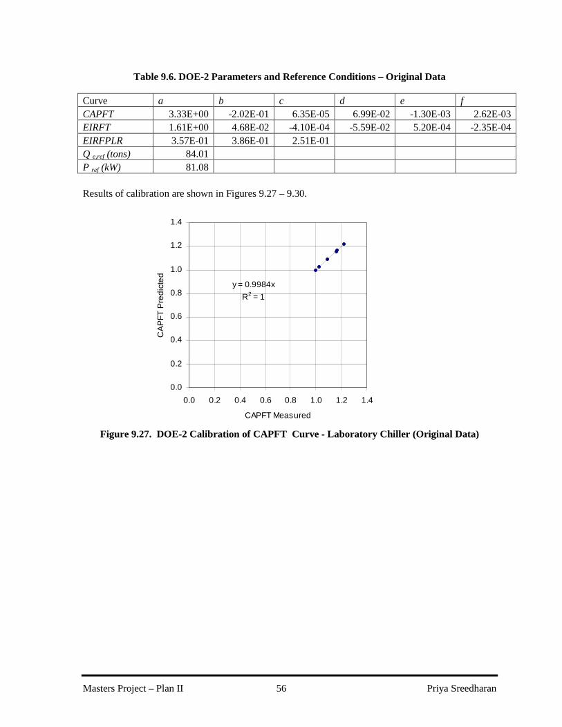
Masters Project – Plan II 56 Priya Sreedharan
Table 9.6. DOE-2 Parameters and Reference Conditions – Original Data
Curve a b c d e f CAPFT 3.33E+00 -2.02E-01 6.35E-05 6.99E-02 -1.30E-03 2.62E-03 EIRFT 1.61E+00 4.68E-02 -4.10E-04 -5.59E-02 5.20E-04 -2.35E-04 EIRFPLR 3.57E-01 3.86E-01 2.51E-01 Q e,ref (tons) 84.01 P ref (kW) 81.08 Results of calibration are shown in Figures 9.27 – 9.30.
y = 0.9984x
R2 = 1
0.0
0.2
0.4
0.6
0.8
1.0
1.2
1.4
0.0 0.2 0.4 0.6 0.8 1.0 1.2 1.4
CAPFT Measured
CA
PF
T P
red
icte
d
Figure 9.27. DOE-2 Calibration of CAPFT Curve - Laboratory Chiller (Original Data)
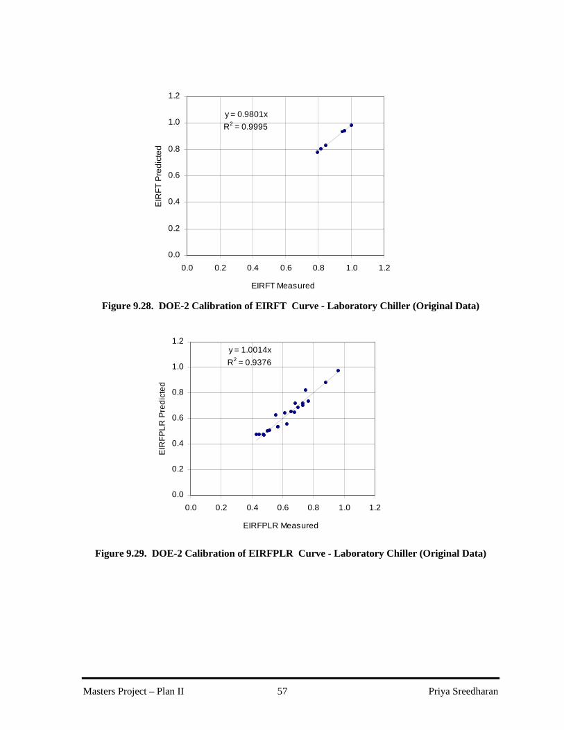
Masters Project – Plan II 57 Priya Sreedharan
y = 0.9801x
R2 = 0.9995
0.0
0.2
0.4
0.6
0.8
1.0
1.2
0.0 0.2 0.4 0.6 0.8 1.0 1.2
EIRFT Measured
EIR
FT
Pre
dic
ted
Figure 9.28. DOE-2 Calibration of EIRFT Curve - Laboratory Chiller (Original Data)
y = 1.0014x
R2 = 0.9376
0.0
0.2
0.4
0.6
0.8
1.0
1.2
0.0 0.2 0.4 0.6 0.8 1.0 1.2
EIRFPLR Measured
EIR
FP
LR
Pre
dic
ted
Figure 9.29. DOE-2 Calibration of EIRFPLR Curve - Laboratory Chiller (Original Data)

Masters Project – Plan II 58 Priya Sreedharan
0
10
20
30
40
50
60
70
80
90
0 10 20 30 40 50 60 70 80 90
Measured Power (kw)
Pre
dict
ed
Pow
er (
kw)
Figure 9.30. DOE-2 Results - Laboratory Chiller (Original Data)
Again, the results for both data sets showed similar trends. As expected, the coefficients were different. Table 9.7 presents the statistical analysis for the model predictions.
Table 9.7. Statistical Analysis of DOE-2 Model Results
Statistical Value Adjusted Data Original Data Average Error (kW) 1.56 2.00 Error (%) 4.56 4.05 r.m.s. error (kW) 1.92 2.42 r.m.s. error (%) 6.02 5.26
Taking into account that the adjusted power measurements were less than the original power measurements, the statistics for both data sets were similar. An uncertainty analysis was performed on the model predictions to determine the influence of the uncertainties of the input data. For this purpose, the original data set was used. As with the other models, the sequential perturbation method was used. The results are presented graphically, as error bars in Figure 9.31.

Masters Project – Plan II 59 Priya Sreedharan
0
10
20
30
40
50
60
70
80
90
0 10 20 30 40 50 60 70 80 90
Measured Power (kw)
Pre
dic
ted
Po
we
r (kw
)
Figure 9.31. DOE-2 Model Results With Uncertainty Error Bars - Laboratory Chiller
The uncertainty in model predictions due to measurement errors in the input data is estimated to be 0.58 kW, or 0.99 %.

Masters Project – Plan II 60 Priya Sreedharan
10. RESULTS – FIELD CASE STUDY
Section 10 includes the analysis of the chiller data obtained from the building chiller over a period of one and half years. Details of the chiller and experimental measurements were given in Section 7.2.
10.1 DATA PROCESSING
10.1.1 FILTERED AND BINNED DATA
Please refer to section 7.2.3 for a more complete description of the data conditioning. The data were first filtered for transients. Although noise is always present in experimental data, the transient effects due to start and shutdown were much larger, and resulted in unrealistic chiller efficiencies. The filtered data set was achieved by increasing the filter parameters, such that the anomalous points with unusual efficiencies were removed. Next, the data were binned by condenser inlet, evaporator outlet temperatures, and evaporator load. The results of the filtering and binning are presented as inefficiency (1/COP) versus evaporator load graphs.
0.00
0.05
0.10
0.15
0.20
0.25
0.30
0.35
0.40
0 100 200 300 400 500 600
Evaporator Load (kW)
1/C
OP
Figure 10.1. Efficiency - Building Chiller - Entire Filtered Unbinned Data Set

Masters Project – Plan II 61 Priya Sreedharan
0.00
0.05
0.10
0.15
0.20
0.25
0.30
0.35
0.40
0 100 200 300 400 500 600
Evaporator Load (kW)
1/C
OP
Figure 10.2. Efficiency - Building Chiller – Filtered Binned Data Set
10.1.2 ENERGY BALANCE AND UNCERTAINTY IN LOAD CALCULATIONS
The energy balance was performed on both the filtered unbinned data set, and filtered binned data set. Figures 10.3 - 10.7 present the results in various modes.
-40
-20
0
20
40
60
80
Time
Bal
ance
(kW
)
Peak Energy Balance due to Evaporator Inlet w ater Sensor failure
Jun-98 Oct-98 Aug-99 Sep-99
Figure 10.3. Energy Balance - Building Chiller Filtered (Unbinned) Data
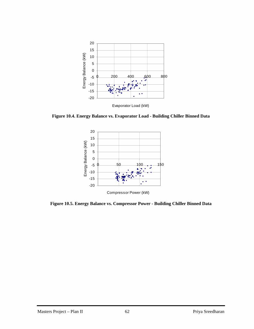
Masters Project – Plan II 62 Priya Sreedharan
-20
-15
-10
-5
0
5
10
15
20
0 200 400 600 800
Evaporator Load (kW)
En
erg
y B
ala
nce
(kW
)
Figure 10.4. Energy Balance vs. Evaporator Load - Building Chiller Binned Data
-20
-15
-10
-5
0
5
10
15
20
0 50 100 150
Compressor Power (kW)
En
erg
y B
ala
nce
(kW
)
Figure 10.5. Energy Balance vs. Compressor Power - Building Chiller Binned Data
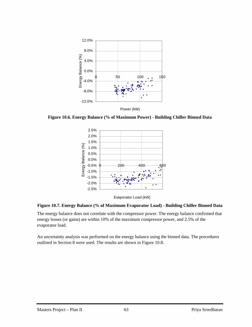
Masters Project – Plan II 63 Priya Sreedharan
-12.0%
-8.0%
-4.0%
0.0%
4.0%
8.0%
12.0%
0 50 100 150
Power (kW)
En
erg
y B
ala
nce
(%
)
Figure 10.6. Energy Balance (% of Maximum Power) - Building Chiller Binned Data
-2.5%
-2.0%
-1.5%
-1.0%
-0.5%
0.0%
0.5%
1.0%
1.5%
2.0%
2.5%
0 200 400 600
Evaporator Load (kW)
En
erg
y B
ala
nce
(%
)
Figure 10.7. Energy Balance (% of Maximum Evaporator Load) - Building Chiller Binned Data
The energy balance does not correlate with the compressor power. The energy balance confirmed that energy losses (or gains) are within 10% of the maximum compressor power, and 2.5% of the evaporator load. An uncertainty analysis was performed on the energy balance using the binned data. The procedures outlined in Section 8 were used. The results are shown in Figure 10.8.

Masters Project – Plan II 64 Priya Sreedharan
-20
-15
-10
-5
0
5
10
15
20
0 20 40 60 80 100
Data Point
Ba
lan
ce (
kW)
Figure 10.8. Energy Balance with Uncertainty Error Bars- Building Chiller Binned Data The uncertainty in energy balance is estimated at ± 2.9 kW.
10.2 ASHRAE TOOLKIT RESULTS
10.2.1 CALIBRATION
The model was calibrated using the binned data set, and both forms of the objective function. The initial parameter values for the Nelder-Mead optimization were chosen as follows: 1) The evaporator conductance (UAe) was estimated using the classical heat exchanger relationships
from (4.2), (4.4), evaporator load (Qe), and an estimated evaporating temperature (Te,ref). 2) The condenser conductance (UAc) was estimated in a similar manner. 3) The Compressor losses proportional to compressor power (α) was simply set to a small number
(0.2). 4) The constant losses from the motor/compressor (Wlo) was set to a small fraction (e.g., 0.2) of the
maximum compressor power (Pcomp,max). Although the Nelder-Mead optimization did not require constraints on the parameters, the following constraints were forced to ensure that the parameters were reasonable: 1) All parameters must be greater than zero. 2) Neither of the heat exchanger conductance's should be larger than the other by more than 150%. 3) The maximum useful compressor work (as calculated using Wlo and α) cannot exceed the
maximum compressor power. 4) proportional losses (α) cannot exceed one.

Masters Project – Plan II 65 Priya Sreedharan
Once the optimization converged, the objective function was confirmed to be a minimum by perturbing the parameters by ±1%. Table 10.1 shows the parameters that were estimated from the measured performance data of the building chiller.
Table 10.1 ASHRAE Toolkit Parameters: Building Chiller
Parameter UAe (kW/K) 54.54 UAc (kW/K) 135.98 α 0.00 Wlo (kW) 41.40 r.m.s. error (kW) 4.09
The shape of the objective function was determined with a range of parameter values for both heat exchanger conductances (UAe and UAc), maintaining the other parameters (Wlo and α) at their optimized values . The surface graph is shown in figure 10.9.
Figure 10.9. ASHRAE Toolkit Results - Building Chiller - Objective Function
The above graph was similar to the shapes determined by the laboratory chiller objective functions, in that, the contour lines showed the expected inverse relationship between the heat exchanger

Masters Project – Plan II 66 Priya Sreedharan
conductances. Surprisingly, the UA's are larger for the laboratory chiller, although the building chiller has a larger capacity (by almost 150%).
10.2.2 MODEL RESULTS
A comparison of the predicted and measured compressor powers for the binned data set is shown in figure 10.10.
0
20
40
60
80
100
120
140
160
0 20 40 60 80 100 120 140 160
Measured Power (kw)
Pre
dic
ted
Po
we
r (kw
)
Figure 10.10. ASHRAE Toolkit Results - Building Chiller
The Toolkit results show a rather significant discontinuity between predicted and measured power at high power (i.e., greater than 105 kW). This discontinuity is discussed in detail in the discussion section. (The discontinuity was found to be present in all the model results, and was not unique to any one model, or even the result of a modeling flaw. Therefore, the discussion was better suited for the discussion section, Section 11.) Table 10.2 presents the statistical analysis for the calibrated model predictions.
Table 10.2. Statistical Analysis of Toolkit Model Results – Binned Data Set
Statistical Value Average Error (kW) 2.97 Error (%) 3.86 r.m.s. error (kW) 4.09 r.m.s. error (%) 4.82
Using the calibration results, the entire unbinned, filtered data set was modeled. A comparison of the predicted and measured compressor powers is shown in figure 10.11.
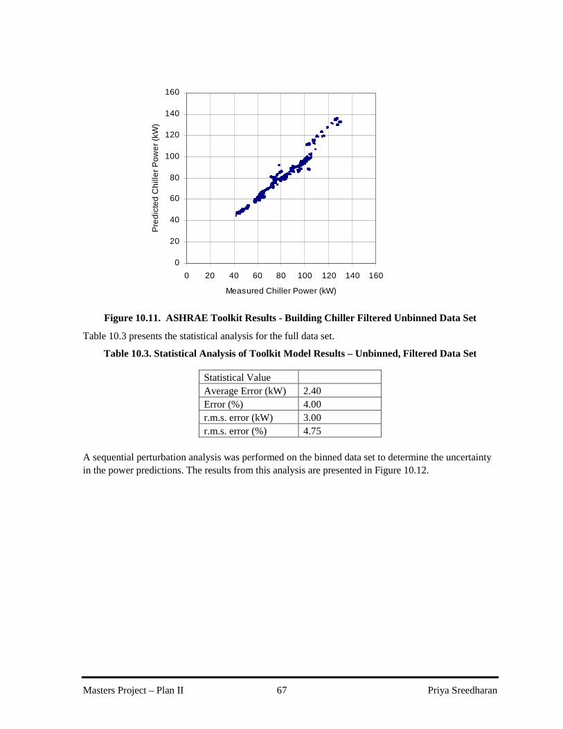
Masters Project – Plan II 67 Priya Sreedharan
0
20
40
60
80
100
120
140
160
0 20 40 60 80 100 120 140 160
Measured Chiller Power (kW)
Pre
dic
ted
Ch
ille
r P
ower
(kW
)
Figure 10.11. ASHRAE Toolkit Results - Building Chiller Filtered Unbinned Data Set
Table 10.3 presents the statistical analysis for the full data set.
Table 10.3. Statistical Analysis of Toolkit Model Results – Unbinned, Filtered Data Set
Statistical Value Average Error (kW) 2.40 Error (%) 4.00 r.m.s. error (kW) 3.00 r.m.s. error (%) 4.75
A sequential perturbation analysis was performed on the binned data set to determine the uncertainty in the power predictions. The results from this analysis are presented in Figure 10.12.

Masters Project – Plan II 68 Priya Sreedharan
0
20
40
60
80
100
120
140
160
0 20 40 60 80 100 120 140 160
Measured Power (kw)
Pre
dic
ted
Po
we
r (kw
)
Figure 10.12. ASHRAE Toolkit Results With Uncertainty Error Bars - Building Chiller
The uncertainty in model predictions due to measurement errors in the input data is estimated to be 0.32 kW, or 0.34 %. This uncertainty is particularly small, and even less than the uncertainty in the flow measurement, because it is biased towards measurements of low power. In the low power regime, a reduction (or increase) in flow, and hence, load, results in a comparatively small decrease (or increase) in power since the efficiency deteriorates rapidly.
10.3 GORDON-NG UNIVERSAL MODEL RESULTS
The Gordon-Ng model is calibrated (parameterized) using linear regression of the term represented in (5.5). The binned data set was used to calibrate the model. The results of this regression are shown in figure 10.13.

Masters Project – Plan II 69 Priya Sreedharan
y = 0.9986x
R2 = 0.9742
0.00
0.05
0.10
0.15
0.20
0.25
0.30
0.35
0.40
0.00 0.05 0.10 0.15 0.20 0.25 0.30 0.35 0.40
y Measured
y P
red
icte
d
Figure 10.13. Gordon-Ng Linear Regression Results - Building Chiller
Table 10.4 shows the parameter sets that were estimated from the measured performance of the laboratory chiller.
Table 10.4 Gordon-Ng Parameters: Building Chiller
Parameter Value ∆ST (kW/K) 0.134 R (K/kW) 0.043 Qleak,eqv (kW) 12.05
The entropy generation for the building chiller is larger than for the laboratory chiller's by 100% for the adjusted data, and 50% for the original data. This can be explained, in part by a larger refrigerant flow rate in the larger chiller. This pattern followed the results found by Ng et. al (1997), where the estimated entropy generation of a 70 kW reciprocating chiller was approximately 500% larger than the entropy generation of a 10 kW reciprocating chiller. The heat loss parameter was 12 kW, which was approximately 7% of the maximum compressor power. This value was low compared to the 40% obtained by Ng et. al (1997), but was more believable than the results obtained for the laboratory chiller. The equivalent heat loss term can be qualitatively compared to the compressor loss term obtained from the Toolkit model. The equivalent heat loss term can be qualitatively compared to the compressor loss term obtained in the Toolkit model. When comparing the results for the adjusted data, the compressor losses from the Toolkit model are larger than the heat leak term found in the Gordon-Ng model. This may be due to the assumption of isentropic compression in the Toolkit model, which is an idealization that must be ‘corrected’ with a larger compressor loss term. This result, however, was not found with the laboratory chiller results.

Masters Project – Plan II 70 Priya Sreedharan
Again, the heat exchanger conductance’s estimated from the Toolkit model were used in combination with the water mass flow rates to estimate an equivalent thermal resistance of 0.034 K/kW. This was slightly less than the 0.043 K/kW obtained from the Gordon-Ng model, but were not significantly different, as was the case with the laboratory chiller. For both the laboratory and building chillers, these thermal resistances are significantly different, although the ranking is the same in each case. Specifically, the thermal resistance for the building was less than that of the laboratory chiller using adjusted data, which in turn was less than the thermal resistance for the laboratory chiller using the original data. Table 10.4 can better demonstrate this point.
Table 10.4. Comparison of Thermal Resistance’s between Toolkit and Gordon-Ng Models
Thermal Resistance (K/kW) Toolkit Gordon-Ng Laboratory Chiller – Original Data
0.040 0.079
Laboratory Chiller – Adjusted Data
0.037 0.051
Building Chiller 0.034 0.043 However, the thermal resistance for the building chiller is not half the resistance for the laboratory chiller, as would be expected based on the capacity difference. Using the estimated parameters, and rearranging (5.5) the compressor power was predicted. The results are shown in Figure 10.14. The variable 'y' is proportional to the inverse of the COP. The lower part of the previous figure showed poor correlation between the predicted y and measured y. The region above the 45° line corresponded to the upper-right region in Figure 10.16 where the measured power was significantly less than the estimated power. The region below the 45° line corresponded to the regions where estimated power was significantly less than the measured power. Both of these regions are marked on figure 10.14. Again, the discontinuity between measured and predicted power at 105 kW is similar to that seen in the Toolkit results. As noted earlier, the discussion section includes an explanation for this discontinuity.

Masters Project – Plan II 71 Priya Sreedharan
0
20
40
60
80
100
120
140
160
0 20 40 60 80 100 120 140 160
Measured Power (kw)
Pre
dic
ted
Po
we
r (kw
)
Figure 10.14. Gordon-Ng Model Results - Building Chiller Binned Data Set
Table 10.5 presents the statistical analysis for the model predictions.
Table 10.5. Statistical Analysis of Gordon-Ng Model Results – Binned Data Set
Statistical Value Average Error (kW) 2.36 Error (%) 2.67 r.m.s. error (kW) 4.01 r.m.s. error (%) 3.86
The unbinned, filtered data set was then modeled using the calibration results, and the results are shown in figure 10.15.

Masters Project – Plan II 72 Priya Sreedharan
0
20
40
60
80
100
120
140
160
0 20 40 60 80 100 120 140 160
Measured Chiller Power (kW)
Pre
dict
ed
Ch
ille
r Po
we
r (k
W)
Figure 10.15. Gordon-Ng Model Results - Building Chiller Filtered Unbinned Data Set
Table 10.6 presents the statistical analysis for the full (filtered) data set.
Table 10.6. Statistical Analysis of Gordon-Ng Model Results- Full Data Set
Statistical Value Average Error (kW) 1.29 Error (%) 1.89 r.m.s. error (kW) 2.34 r.m.s. error (%) 2.87
An uncertainty analyses of the model predictions, due to experimental error was performed using the sequential perturbation method. The results are presented graphically, as error bars in Figure 10.16.

Masters Project – Plan II 73 Priya Sreedharan
0
20
40
60
80
100
120
140
160
0 20 40 60 80 100 120 140 160
Measured Power (kw)
Pre
dic
ted
Po
we
r (kw
)
Figure 10.16. Gordon-Ng Model Results With Uncertainty Error Bars -Building Chiller
The uncertainty in model predictions due to measurement errors in the input data is estimated to be 0.37 kW, or 0.40 %.
10.4 COOLTOOLS/DOE-2 MODEL RESULTS
Since full load data for the building chiller were unavailable, the CoolTools software was used to select a chiller curves that have already been fitted to the DOE-2 model. Each parameter set in the library is tested using data from the chiller to be calibrated and the curve producing the lowest r.m.s. error is selected. Table 10.7 lists the reference conditions and parameters estimated by the CoolToolsTM automated calibration procedure from the measured performance of the building chiller.
Table 10.7. CoolTools Automated Calibration Parameters and Reference Conditions
Curve a b c d e f CAPFT 7.25E-01 4.67E-03 -7.40E-05 4.24E-03 -3.01E-05 2.95E-05 EIRFT 1.07E+00 -1.50E-02 4.96E-04 5.95E-03 2.22E-04 -5.76E-04 EIRFPLR 3.05E-01 2.76E-01 4.18E-01 Qe,ref (tons) 160.68 P,ref (kW) 108.72 A comparison of measured and predicted compressor powers using the binned data set is shown in figure 10.17.

Masters Project – Plan II 74 Priya Sreedharan
0
20
40
60
80
100
120
140
160
0 20 40 60 80 100 120 140 160
Measured Power (kw)
Pre
dic
ted
Po
we
r (kw
)
Figure 10.17. CoolTools/DOE-2 Results - Building Chiller Binned Data Set
The results closely resemble the results from the other models. Interestingly, all three models show a discontinuity between measured and predicted power at 105 kW. The similarities between all three model results are discussed in Section 11, as well explanations for the discontinuity. Table 10.8 presents the statistical analysis for the binned data model predictions.
Table 10.8. Statistical Analysis of CoolTools/Doe-2 Model Results- Automated Calibration (Binned Data Set)
Statistical Value Average Error (kW) 2.45 Error (%) 2.73 r.m.s. error (kW) 4.24 r.m.s. error (%) 4.03
The unbinned filtered data set was then modeled using the calibration results, and are shown in figure 10.18.

Masters Project – Plan II 75 Priya Sreedharan
0
20
40
60
80
100
120
140
160
0 20 40 60 80 100 120 140 160
Measured Chiller Pow er (kW)
Pre
dict
ed C
hille
r P
ower
(kW
)
Figure 10.18. CoolTools/DOE-2 Results - Building Chiller Filtered Unbinned Data Set
Table 10.9 presents the statistical analysis for the unbinned filtered data set.
Table 10.9. Statistical Analysis of CoolTools/DOE-2 Model Results- Full (Unbinned & Filtered) Data Set
Statistical Value Average Error (kW) 1.31 Error (%) 1.90 r.m.s. error (kW) 2.40 r.m.s. error (%) 2.86
An uncertainty analysis was performed on the model predictions to determine the influence of the uncertainty of the input data. This was determined from the binned data set. Again, the sequential perturbation method was used. The results are presented graphically, as error bars in Figure 10.19.

Masters Project – Plan II 76 Priya Sreedharan
0
20
40
60
80
100
120
140
160
0 20 40 60 80 100 120 140 160
Measured Power (kw)
Pre
dic
ted
Po
we
r (kw
)
Figure 10.19. CoolTools/DOE-2 Results With Uncertainty Error Bars - Building Chiller
The uncertainty in model predictions due to measurement errors in the input data is estimated to be 0.367 kW, or 0.41 %.

Masters Project – Plan II 77 Priya Sreedharan
11. DISCUSSION
11.1 SUMMARY OF RESULTS AND GENERAL OBSERVATIONS
Table 11.1 contains a summary of the r.m.s. error's of the model predictions, as well as the r.m.s. error's of the uncertainty in the model predictions due to measurement error. The results for the building chiller are based on the binned data set.
Table 11.1 Summary of Modeling Results
Model Prediction Error (kW) Model Prediction Uncertainty (kW)
Laboratory Chiller Model Adjusted Data
Original Data
Building Chiller
Laboratory Chiller (original data)
Building Chiller
ASHRAE Toolkit
1.34 1.95 4.09 0.83 0.32
Gordon-Ng 1.38 2.21 4.01 0.68 0.37 DOE-2/ CoolTools
1.92 2.42 4.24 0.58 0.37
Based on the statistical analyses, the accuracy of the physical models (i.e., ASHRAE Toolkit, Gordon-Ng) as indicated by the r.m.s. error is similar, and within 0.04 kW for the adjusted data, and 0.26 kW for the original data (where the adjusted data corrected the compressor power measurements for energy losses to the environment). The ASHRAE Toolkit performed slightly better in the case of the laboratory chiller, while the Gordon-Ng model performed slightly better with the building chiller. The empirical model results (i.e., DOE-2/CoolTools) were only slightly less accurate than the physical model results. The uncertainty in the model predictions due to experimental error was calculated using the sequential perturbation method. This method basically varied each input data by the maximum error of that sensor, one by one, to compute the individual uncertainties, from which the overall uncertainty was computed. This uncertainty was minimal, which was not surprising, as both projects used high-quality temperature and flow sensors. LABORATORY CHILLER: The trends between the physical models are similar. However, the trends seen with empirical model results differed. This was a direct consequence of the calibration method, which separately used the full load and part load data. The CoolTools software was very successful in calibrating the building chiller data to the DOE-2 curves; the CoolTools library, which contains over one-hundred pre-calibrated chiller curves, allows the calibration of part-load data possible.

Masters Project – Plan II 78 Priya Sreedharan
BUILDING CHILLER RESULTS: All three model results show similar trends. In particular, a significant discontinuity between the predicted and measured compressor power at 105 kW is observed with all three models. In addition, data taken from the backup chiller in the building showed a similar pattern. This discontinuity, however, was not observed with the laboratory chiller’s results. This is discussed further in section 11.4. PARAMETER COMPARISON: Table 11.2 lists the various parameters estimated from the physical models. 'TK' refers to the Toolkit Model, and 'G-Ng' refers to the Gordon-Ng model.
Table 11.2. Summary of Parameter Estimates
Laboratory Chiller
Adjusted Data Original Data
Building Chiller
Wlo – TK (kW) 18.09 26.82 41.40 α − ΤΚ (−−) 0.00 0.28 0.00 UAe – TK (kW/K) 92.49 68.54 54.54 UAc – TK (kW/K) 170.37 171.36 135.98 R – TK (K/kW) 0.037 0.040 0.034 R – G-Ng (K/kW) 0.051 0.079 0.043 ∆ST (kW/K) 0.058 0.080 0.134 Qleak (kW) 35.26 105.65 12.05
The laboratory chiller data exhibits significant energy losses from the compressor to the environment. Energy losses, as a percentage of compressor consumption, tend to be larger with smaller chillers (Bourdouxhe,1994). The compressor power measurements were corrected for the proportional electromechanical compressor losses, and both this corrected data set, and the original data set were used to calibrate all three models. While the accuracy of the model predictions was not affected by the electromechanical losses, the estimated heat leak parameter, from the Gordon-Ng model is significantly larger, as a percentage of compressor capacity, compared to the building chiller, and other studies (Ng, 1997). An unusual result is that the Toolkit model estimated larger conductance’s (UA’s) for the laboratory chiller, although the building chiller had more than twice the capacity. The thermal resistance’s as defined by the Gordon-Ng model are closer to expected behavior, although the thermal resistance of the laboratory chiller is only slightly larger than the thermal resistance estimated for the building chiller. The thermal resistance calculated from the Toolkit parameters does not match those from the Gordon-Ng model. This may be attributed to the treatment of environmental losses. The Gordon-Ng model estimates energy losses to the environment, whereas, the Toolkit model loses energy solely through the condenser, which accounts for the smaller thermal resistance’s from the Toolkit model. However, the thermal resistance estimated from the Gordon-Ng model corroborated this result. The loss parameters from both models followed expected behavior. In the case of the building chiller, the compressor loss term from the Toolkit model is larger than the leak term from the Gordon-Ng model. This is not the case for the laboratory chiller results. This results may be explained by the isentropic compression assumption in the Toolkit model, an idealization that is ‘corrected’ with a larger loss term. The leak term obtained from the Gordon-Ng model when using the original data is

Masters Project – Plan II 79 Priya Sreedharan
unreasonably large. This questions the Gordon-Ng model's ability to treat chillers with environmental losses proportional to the compressor power.
11.2 MODEL LIMITATIONS
This section discusses the assumptions and limitations of each model.
11.2.1 ASHRAE TOOLKIT MODEL
The following assumptions are made in the formulation of the model: ¾ Losses to environment are considered negligible. ¾ Motor inefficiencies are modeled completely as sensible heat gain by the refrigerant, prior to
compression. ¾ The refrigerant in the compressor is treated as an ideal gas. ¾ De-superheating and sub-cooling in the condenser are ignored, resulting in an inflated condenser
heat transfer coefficient. ¾ For centrifugal compressors, compression work is considered isentropic at full-load and part-load. ¾ Calibration of the original model for centrifugal chillers requires full-load data. In addition to the above assumptions, one more assumption was made in order to convert the model into a universal chiller model, independent of compressor type, and slightly altered the original equations: The Toolkit authors modeled the part-load condition as a throttling process prior to compression. This pressure drop resulted in an increase in the specific volume of the refrigerant, which in turn achieved a reduced refrigerant flow rate. The reduced or "part-load" refrigerant flow rate was then used to compute work input to the compressor. Since the original model structure maintained both compressor power and evaporator load as 'outputs', this "throttling" was the only way to force part-load conditions. However, in converting the model to a usable form, it was restructured, such that compressor power was an input, and evaporator load an output, and then, again, such that power was the output (to match the other models). In computing refrigerant flow rate from useful compressor work, the specific volume of the refrigerant, in the absence of such a throttling process was used. The limitations found with this model as applied in this study include: ¾ Calibration is achieved through the Nelder-Mead direct search method, which is considerably
more time-consuming and involved than simple linear regression. ¾ The model equations are solved in an iterative manner, and convergence, while improved using
the secant method, is not always guaranteed. ¾ Refrigerant thermodynamic properties are required.
11.2.2 GORDON-NG MODEL
The Gordon-Ng model formulation is similar to the Toolkit model in some aspects, but different in others (see Section 5.3 for a comparison between the models) . Unlike the Toolkit model, which is a component based approach, the Gordon-Ng model is a systems approach. The model has the following limitations:

Masters Project – Plan II 80 Priya Sreedharan
¾ While the Toolkit model neglects environmental losses, the Gordon-Ng model estimates an average equivalent energy leak (a combination of evaporator and compressor losses). However, this quantity does not adequately account for losses proportional to compressor power.
¾ Unlike the Toolkit model, this version of the model does not incorporate variable evaporator and condenser flow rate, however the model authors have devised an alternate form to incorporate variable condenser flow rate.
¾ The total thermal resistance is estimated, and represents the sum of the condenser and evaporator resistances. The effectiveness of each heat exchanger is not evaluated.
11.2.3 DOE-2 / COOLTOOLS MODEL
The following limitations were found with the DOE-2/CoolTools model: ¾ Although the CoolTools calibration was very successful for the building chiller, it is not clear
how much data are required for a successful calibration. ¾ The parameters have no physical meaning. ¾ Condenser and evaporator flow rate were assumed constant, and therefore is not valid for chillers
with variable water flow rate.
11.3 BUILDING CHILLER MODEL PREDICTION DISCONTINUITY
A strange discontinuity is observed in the all three sets of modeling results for the building chiller. This discontinuity was not present in the laboratory chiller model results. The model residuals were compared with energy balance, and the condenser and evaporator inlet temperature difference, which is an indicator of pressure lift.
-20
-15
-10
-5
0
5
10
15
0 5 10 15 20
Tci-Tei (k)
Re
sid
ua
l (kw
)
Figure 11.7. Residual vs. Temperature Lift – Building Chiller Binned Data

Masters Project – Plan II 81 Priya Sreedharan
-20
-15
-10
-5
0
5
10
15
-20 -15 -10 -5 0
Energy Balance (kW)
Re
sid
ua
l (kw
)
Figure 11.8. Residual vs. Energy Balance – Building Chiller Binned Data
Figures 11.7 and 11.8 demonstrated a strong correlation between residual and temperature difference, but not with energy balance. The residuals were significantly larger at the highest temperature differences. Further analysis showed that the chiller was operating more efficiently in the high power regions where this greater temperature difference existed, than would be expected for those particular operating conditions. Figure 11.9 shows the measured chiller efficiency (1/COP) as a function of evaporator load. The difference between the evaporator water inlet temperature and condenser water inlet temperature is scaled and is also shown on the figure.

Masters Project – Plan II 82 Priya Sreedharan
0.00
0.05
0.10
0.15
0.20
0.25
0.30
0.35
0.40
0 200 400 600 800
Evaporator Load (kW)
1/C
OP
1/COP
(Tci-Tei) Scaled
Figure 11.9. Measured Efficiency – Building Chiller Binned Data
Consider the circled portion in the figure: Based on the increase in temperature difference between the evaporator and condenser inlet water conditions, there appears to be a pressure increase in this circled region. However, this ‘pressure increase’ did not cause a decrease in efficiency, as would be suspected. Note, the '1/COP' graph did not show a similar type of discontinuity. However, the models would expect power consumption to increase with an increase in pressure lift, which explains the discontinuity in the model results. Currently, there is no explanation for the chiller operating more efficiently than would be expected in this region. We are pursuing this problem with chiller manufacturers and hope to have closure in the near future.
11.3.1 LARGE RESIDUALS IN THE BUILDING MODEL PREDICTIONS (FULL DATA SET)
All three models exhibited similar regions of high residuals, where model prediction error was significantly large. In an FDD scheme, these large residuals would trigger the possibility of a fault. It was therefore important to identify whether these residuals were caused by faults, or were due to inadequacies in the model(s). It was found that each grouping of residuals came from a particular day of chiller operation. All but one of the residual groups found from the model predictions graph (s) were also identified as isolated data groups in the efficiency curves. This is most easily explained with the aid of figures. Refer to figures 11.10 and 11.11 to see which dates correspond to the various irregular groups.

Masters Project – Plan II 83 Priya Sreedharan
0
20
40
60
80
100
120
140
160
0 20 40 60 80 100 120 140 160
Measured Chiller Power (kW)
Pre
dict
ed
Ch
ille
r Po
we
r (k
W)
7/7/98
4/16/99
7/7/99,7/12/99
4/14/99
Figure 11.1. Residual Analysis – Gordon-Ng Model Results - Building Chiller Filtered Data
0.00
0.05
0.10
0.15
0.20
0.25
0.30
0.35
0.40
0 100 200 300 400 500 600
Evaporator Load (kW)
1/C
OP
7/7/98
4/16/99
4/14/997/7/99, 7/12/99
9/27/99
Figure 11.2. Residual Analysis - Efficiency - Building Chiller Filtered Data
The sensor failure from July 7, 1998 was identified earlier, and accounts for the low power (less than 100 kW) positive residuals (predicted power greater than measured power). Recall, the other set of positive residuals at high power was discussed earlier. The remainder of the residuals could not be explained either by a sensor failure, which would have been observable from the energy balance. In

Masters Project – Plan II 84 Priya Sreedharan
these cases, the modeled residuals were accompanied by efficiency deviations on figure 11.11. Each of these groups were compared with points of similar evaporator load to determine if the chiller was operating in an expected manner. It was found that the greater inefficiencies found on April 16, July 7 and 12, 1999 could partially be explained by a decrease in evaporator temperatures, and/or increase in condenser temperatures (indicating an increase in pressure lift), which would indicate an increase in power. However, the model predictions showed that these power differences (when compared with operating days of similar evaporator load) should not have been quite as large as they were. In addition to the lower evaporator water temperatures, the evaporator water flow rate from April 16 was significantly less than on September 17, 1998, the date used for comparison purposes. The evaporator temperature difference was larger to compensate for the reduction in flow rate, such that evaporator loads were still equivalent between the two days. The measurements demonstrated that in order to achieve a similar evaporator load, with reduced flow rate, the refrigerant must be cooled to a lower temperature or its flow rate must be increased to cool the evaporator water to a lower temperature, resulting in an increase in compressor power. Neither the CoolTools, or Gordon-Ng models account for variable evaporator water flow rates,15 which explains why the predicted power from those models were less than the measured power. The Toolkit model, which does account for variable evaporator flow rate did predict lower power, but was closer to the actual power measurement. Since 95% of the filtered data had evaporator flow rates that were within one standard deviation of the average flow rates, this factor alone need not favor the Toolkit model over the other models. The residuals from April 14, 1999 could not be explained. When the operating conditions were compared with those of October 20, 1998 (which had a similar evaporator load) it was found that the evaporator temperatures were slightly larger on April 14, which should have resulted in lower inefficiency on April 14. The actual measurements, however, showed smaller inefficiencies for October 20, contradicting the hypothesis based on the evaporator conditions. This explained why the predicted power measurements were smaller than the actual measurements on April 14; in fact, the predicted power measurements were smaller for April 14, than for October 20. In summary, many of the residuals were caused by anomalous behavior of the chiller, rather than by limitations of the models. Further consultation with industry experts may help to explain the patterns in efficiency that did not follow expected behavior. In addition, examination of another year of data from this same chiller may be helpful, as well as examination of operating data from a different building chiller. Refrigerant measurements may also help diagnose such behavior, and could be used to build a more robust component modeling scheme.
15 Although, (Gordon, 1999) addressed variable condenser flow rate, and modified their model accordingly. The
new model became non-linear in the parameters.

Masters Project – Plan II 85 Priya Sreedharan
12. CONCLUSIONS
The ability of the models to reproduce the observed behavior, as indicated by the r.m.s. prediction errors, is quite similar. The similarity of the graphs of predicted vs. measured power indicates that the dominant sources of error are either in the measurements or result from behavior that none of the models treat. The variation in the parameter values from model to model and chiller to chiller can be explained in terms of the assumptions of the models. ¾ The isentropic compression assumption in the Toolkit model results in a larger estimate for the
loss term, as compared to the Gordon-Ng model, which accounts for entropy generation in compression.
¾ The Gordon-Ng model's assumption of constant heat losses/gains over the operating range results in unreasonably large estimates of the leak parameter, questioning the ability of this model to treat chillers with heat losses proportional to compressor power.
¾ The Toolkit model, as used in this study, produced larger estimates of the heat exchanger coefficients (UA's) for the laboratory chiller, although the building chiller had a significantly larger cooling capacity. The estimates of thermal resistance, as defined in the Gordon-Ng model, were larger for the laboratory chiller, though not as large as would be expected from the difference in the cooling capacities of the two chillers
Of the first principles models, the Gordon-Ng model has the advantage of being linear in the parameters, which allows more robust parameter estimation methods to be used and facilitates estimation of the uncertainty in the parameter values. The ASHRAE Toolkit Model may have advantages when refrigerant temperature measurements are also available since it should be possible to predict the expected performance of the compressor, condenser and evaporator separately with more confidence, and with more meaningful parameter estimates, than has been found to be possible with only water side thermal measurements. The DOE-2 model can be expected to have advantages when very limited data are available to calibrate the model, as long as one of the previously identified models in the CoolTools library matches the performance of the chiller in question. None of the models could explain the anomalous behavior of the building chiller, which showed a significant discontinuity between predicted and measured compressor powers at high power. The chiller appeared to be performing more efficiently than would be expected based on the operating conditions. A more robust modeling approach, that incorporates internal, refrigerant measurements may explain such behavior.

Masters Project – Plan II A - 1 Priya Sreedharan
ACKNOWLEDGEMENTS
I'd first like to thank both my advisors, Professor Van Carey from the Mechanical Engineering Department at Cal, and Dr. Philip Haves from Lawrence Berkeley Laboratory. I'd also like to thank Mary Ann Piette, and Saki Kinney, also from LBL for providing me with the building chiller data. Thanks are also due to James Braun of Purdue University for providing the performance data for the laboratory chiller. Last, but not least, I'd like to thank Professor David Auslander for agreeing to review this very lengthy report, and be second chair on the review committee. This work was completed under contract to Lawrence Berkeley National Laboratory as part of the High Performance Commercial Building Systems program. This program is supported by the California Energy Commission's Public Interest Energy Research (PIER) Buildings Program and the Assistant Secretary for Energy Efficiency and Renewable Energy, Office of Building Technology, Building Technologies Program, of the U.S. Department of Energy under Contract No. DE-AC03-76SF00098.

Masters Project – Plan II A - 2 Priya Sreedharan
REFERENCES
Bourdouxhe, J. P., M. Grodent, J. J. Lebrun. 1994. "A Toolkit for Primary HVAC System Energy Calculation – Part 2: Reciprocating Chiller Models", ASHRAE Transactions, vol. 100, Part 2, pp. 774-786. Bourdouxhe, J. P., M. Grodent, J. J. Lebrun. 1994. "A Toolkit for Primary HVAC System Energy Calculation", Draft Final Report prepared for The American Society of Heating, Refrigerating and Air Conditioning Engineers. Braun, J. B., E. A. Groll, S. Bendapudi. 2000. "Steady-state model of a centrifugal chiller", Purdue University. (not published) Braun, J. 1999. "Automated Fault Detection and Diagnostics for the HVAC&R Industry", International Journal of HVAC&R Research, vol. 5, no.2, pp. 85-86. Browne, M. W., P.K. Bansal, 1998. "Challenges in Modeling Vapor-Compression Liquid Chillers,” ASHRAE Transactions, Vol. 104, Part 1a, pp. 474-486. Chua, H. T. , K. C. Ng, J. M. Gordon. 1996. "Experimental study of the fundamental properties of reciprocating chillers and their relation to thermodynamic modeling and chiller design", International Journal of Heat and Mass Transfer, vol. 39, no. 11, pp. 2195-2204. Comstock, M., J. E. Braun, 1999. "Development of Analysis Tools for the Evaluation of Fault Detection and Diagnostics in Chillers”, Ray W. Herrick Laboratories Report #4036-3. Figliola, R., S., D. E. Beasley. 1995. Theory and design for mechanical measurements (Second Edition). John Wiley & Sons, Inc., NY. Gordon, J. M., K. C. Ng, H. T. Chua, C. K. Lim. 2000. "How varying condenser coolant flow rate affects chiller performance: thermodynamic modeling and experimental confirmation", Applied Thermal Engineering, vol. 20, pp. 1149-1159. Gordon, J. M., K. C. Ng. 1995. "Predictive and diagnostic aspects of universal thermodynamic model for chillers", International Journal of Heat and Mass Transfer, vol.38, no.5, pp. 807-818. Gordon, J., K. C. Ng. 2000. Cool Thermodynamics. Cambridge International Science Publishing. UK. Haves, P., S. Khalsa. 2000. "Model-based Performance Monitoring: Review of Diagnostic Methods and Chiller Case Study", Proc. ACEEE Summer School, Asilomar, CA, August, LBNL Report 45949

Masters Project – Plan II A - 3 Priya Sreedharan
Haves, P. 1999. "Overview of Diagnostics Methods", Proceedings of Diagnostics for Commercial Buildings: From Research to Practice, San Francisco, CA. http:/poet.lbl.gov/diagworkshop/proceedings/haves.htm Isermann, R., P. Balle. 1997. "Trends in the application of model-based fault detection and diagnosis of technical processes", Control Engineering Practice, vol.5, no.5, pp. 709-719. Meyers, S. R. 1996. "Chiller Modeling Error Analysis: Implications for Energy-savings Retrofits and Control Strategies", Masters Thesis, University of California, Berkeley. Nelder, J. A., R. Mead. 1965. "A Simplex method for function minimization", The Computer Journal, vol. 8, pp. 308-313. Ng, K. C., H. T. Chua, W. Ong, S. S. Lee, J. M. Gordon. 1997. "Diagnostics and optimization of reciprocating chillers: theory and experiment", Applied Thermal Engineering, vol. 17, no. 3, pp. 263-276. Pacific Gas and Electric, 1996. Proceedings from the PG&E Energy Center DOE-2 Lunch Series: Chiller Plant Performance Curves, San Francisco, CA. Peitsman, H. C., V. E. Bakker. 1996. "Application of Black-Box Models to HVAC Systems for Fault Detection", ASHRAE Transactions, vol. 102, Part 1, pp. 628-640. Phelan, J., M. J. Brandemuehl, M. Krarti. 1997. "In-Situ Performance Testing of Chillers for Energy Analysis", ASHRAE Transactions, vol. 103, Part 1, pp. 290-302. Piette, M. A., S. Khalsa, P. Rumsey, K. L. Kinney, E. L. Lee, A. Sebald, and C. Shockman. 1998. "Early Results and Field Tests of an Information Monitoring and Diagnostic System for Commercial Buildings", prepared for the California Energy Commission and the California Institute for Energy Efficiency, LBNL 42338, September. Downloadable from http://poet.lbl.gov/imds/phase2/ Piette, M. A., S. Khalsa, P. Haves, P. Rumsey, K. L. Kinney, E. L. Lee, A. Sebald, and C. Shockman. 1999. "Performance Assessment and Adoption Processes of an Information Monitoring and Diagnostic System Prototype", Report to the California Energy Commission and LBNL 44453. Reddy, A., D. Niebur, J. Gordon, J. Seem, 2000. “Literature Review and Formulation of Research Plan: Development and Comparison of On-Line Model Training Techniques for Model-Based FDD Methods Applied to Vapor Compression Chillers,” Draft report submitted to ASHRAE, for ASHRAE Research Project 1139-RP. Schwefel, H. P. 1995. Evolution and Optimum Seeking. John Wiley & Sons, Inc., NY.