Evaluation of Cloud Fraction Simulated by Seven SCMs against theARM Observations at the SGP Site*

HUA SONG,1 WUYIN LIN,1 YANLUAN LIN,# AUDREY B. WOLF,@ LEO J. DONNER,&

ANTHONY D. DEL GENIO,** ROEL NEGGERS,11 SATOSHI ENDO,1 AND YANGANG LIU1

1Brookhaven National Laboratory, Upton, New York#Ministry of Education Key Laboratory for Earth System Modeling, Center for Earth System Science,

Tsinghua University, Beijing, China@Columbia University, New York, New York

&NOAA/Geophysical Fluid Dynamics Laboratory, Princeton, New Jersey

** NASA Goddard Institute for Space Studies, New York, New York11Royal Netherlands Meteorological Institute, De Bilt, Netherlands

(Manuscript received 9 September 2013, in final form 2 June 2014)

ABSTRACT

This study evaluates the performances of seven single-column models (SCMs) by comparing simulated cloud

fraction with observations at the Atmospheric RadiationMeasurement Program (ARM) SouthernGreat Plains

(SGP) site fromJanuary 1999 toDecember 2001. Comparedwith the 3-yrmean observational cloud fraction, the

ECMWF SCM underestimates cloud fraction at all levels and the GISS SCM underestimates cloud fraction at

levels below 200hPa. The two GFDL SCMs underestimate lower-to-middle level cloud fraction but over-

estimate upper-level cloud fraction. The three Community Atmosphere Model (CAM) SCMs overestimate

upper-level cloud fraction and produce lower-level cloud fraction similar to the observations but as a result of

compensating overproduction of convective cloud fraction and underproduction of stratiform cloud fraction.

Besides, the CAM3 and CAM5 SCMs both overestimate midlevel cloud fraction, whereas the CAM4 SCM

underestimates. The frequency and partitioning analyses show a large discrepancy among the seven SCMs:

Contributions of nonstratiform processes to cloud fraction production are mainly in upper-level cloudy events

over the cloud cover range 10%–80% in SCMswith prognostic cloud fraction schemes and in lower-level cloudy

events over the cloud cover range 15%–50% in SCMs with diagnostic cloud fraction schemes. Further analysis

reveals different relationships between cloud fraction and relative humidity (RH) in the models and observa-

tions. The underestimation of lower-level cloud fraction in most SCMs is mainly due to the larger threshold RH

used inmodels. The overestimation of upper-level cloud fraction in the threeCAMSCMs and twoGFDLSCMs

is primarily due to the overestimation of RH and larger mean cloud fraction of cloudy events plus more

occurrences of RH around 40%–80%, respectively.

1. Introduction

Clouds are a major source of uncertainty in future cli-

mate change projections (e.g., Cess et al. 1996; Solomon

et al. 2007; Boucher et al. 2014). This motivates the

quantitative evaluations of clouds in climate models

against in situ and remote sensing observational data. A

key question is how to use the increasingly available

observational data to efficiently evaluate the perfor-

mance of climate models in representing clouds. Testing

the treatment of cloud-related physical processes in full

general circulation models (GCMs) is both scientifically

and computationally demanding. An alternative approach

is the use of single-column models (SCMs): namely, mod-

eling the atmosphere in a single column of climate models

(Randall et al. 1996).

With the collective effects of the surrounding grid

columns being constrained by observations, the SCM-

based approach has proven to be a powerful tool for

* Supplemental information related to this paper is available at

the Journals Online website: http://dx.doi.org/10.1175/JCLI-D-13-

00555.s1.

Corresponding author address:Hua Song, Atmospheric Sciences

Division, Brookhaven National Laboratory, 75 Rutherford Dr.,

Bldg. 815E, Upton, NY 11973-5000.

E-mail: hsong@bnl.gov; lyg@bnl.gov

6698 JOURNAL OF CL IMATE VOLUME 27

DOI: 10.1175/JCLI-D-13-00555.1

� 2014 American Meteorological Society

evaluating parameterizations of subgrid-scale processes

(i.e., Neggers et al. 2012; Zhang et al. 2013) and has been

adopted by several major scientific programs, including

the Global Energy and Water Cycle Experiment

(GEWEX) Cloud System Study (GEWEX Cloud Sys-

tem Science Team 1993) and the U.S. Department of

Energy’s Atmospheric Radiation Measurement Pro-

gram (ARM; Stokes and Schwartz 1994; Ackerman and

Stokes 2003) and Atmospheric System Research (ASR)

program. ARM/ASR has organized a series of SCM

intercomparison studies using observations at the ARM

sites. Most of these studies are focused on specific cases

over a week- or month-long periods (e.g., Ghan et al.

2000; Xie et al. 2002, 2005; Xu et al. 2005; Klein et al.

2009; Morrison et al. 2009; Davies et al. 2013). However,

to make a statistically meaningful comparison and

evaluation of model performance, longer SCM simu-

lations are desirable. To carry out long-term SCM

simulations, one must obtain the reliable long-term

large-scale advective tendency (forcing) data. ARM

has constructed the multiyear continuous large-scale

forcing data over the ARM Southern Great Plains

(SGP) site, using an objective variational analysis

method and constrained by the surface and top-of-the-

atmosphere observations (Xie et al. 2004). Forced with

these continuous forcing data, several-year-long SCM

simulations of the Goddard Institute for Space Studies

(GISS) model at the ARM SGP site have been used to

analyze cloud feedbacks by Del Genio et al. (2005) and

to evaluate the model performance on cloud simula-

tions by Kennedy et al. (2010). Using these observa-

tionally constrained continuous large-scale forcing

data, we have carried out 3-yr (1999–2001) simulations

of seven GCMs participating in the Fast-Physics Sys-

tem Testbed and Research (FASTER) project at the

ARM SGP site, with the aid of the FASTER SCM test

bed. Detailed information on the FASTER project and

the test bed can be found online (at http://www.bnl.gov/

faster/). In our previous study (Song et al. 2013), eval-

uation of precipitation in the 3-yr SCM simulations

using the ARM observations shows that, although the

seven SCMs can produce the observed precipitation

reasonably well, they differ tremendously in details and

suffer from compensating errors between precipitation

intensity and frequency. The different SCM perfor-

mances and associations with large-scale forcing and

thermodynamic factors shed useful insights on con-

vection parameterizations and future development. To

further expose the parameterization deficiencies, this

paper focuses on evaluation of cloud fraction.

Accurate simulation of the vertical structure of cloud

fraction in amodel is critical to understand cloud feedback

processes. The vertical distribution of clouds may affect

the vertical heating profiles through radiative and latent

heating processes and thus influence the atmospheric

stratification and general circulation (e.g., Stephens et al.

2002). Qian et al. (2012) evaluated the cloud fraction

simulated in the Intergovernmental Panel on Climate

Change (IPCC) FourthAssessmentReport (AR4)GCMs

at three ARM sites, demonstrating the significant differ-

ences in the model performances of cloud simulation at

different vertical levels and different sites. Kennedy et al.

(2010) showed that the simulated clouds at different levels

in the GISS SCM are differently biased from the surface

and satellite observations and also revealed the different

dependences of the modeled high and low clouds on the

large-scale synoptic patterns and variables.

This study evaluates some key features (vertical pro-

files, amounts, and frequencies) of cloud fraction simu-

lated by seven SCMs against the ARM observations at

the SGP site. We first examine the seasonal and diurnal

variations of cloud fraction and illustrate the striking

differences in the vertical structures of cloud fraction

between the SCMs and observations and among the

SCMs. We then analyze the possible factors that could

contribute to these differences through partitioning the

nonstratiform and stratiform cloudy events in the seven

SCMs. Last, we investigate the possible influences of

relative humidity on the model biases of cloud fraction

in connection with model parameterizations. The rest of

the paper is organized as follows: Section 2 describes the

models and data used in this study. The main results are

presented in sections 3–6. Section 7 summarizes the

major conclusions.

2. Model description and evaluation data

a. Participating models

Three main U.S. GCMs [the Community Atmosphere

Model (CAM), the Geophysical Fluid Dynamics Lab-

oratory (GFDL) Atmospheric Model (AM), and the

Goddard Institute for Space Studies (GISS) Model

E2] and one European GCM [the European Centre

for Medium-Range Weather Forecasts (ECMWF) In-

tegrated Forecast System (IFS)] participate in the

FASTER project. To further enhance the diagnosis of

parameterizations and track the model improvement,

the CAM and GFDLAM also include multiple versions

(CAM3, CAM4, and CAM5; AM2 andAM3). Note that

the GFDL AM3 used here is not the full version of

GFDL AM3 (Donner et al. 2011). Here, the major

change of the AM3 from the AM2 is the convection

scheme. The AM2 uses the relaxed Arakawa–Shubert

scheme (Moorthi and Suarez 1992) for both deep and

shallow convections while the AM3 uses the Donner

1 SEPTEMBER 2014 SONG ET AL . 6699

cumulus scheme (Donner et al. 2001, 2011) for deep

convection andUniversity ofWashington (UW) scheme

(Bretherton et al. 2004) for shallow convection. Table 1

summaries the sevenGCMs used in the intercomparison

study, including the number of vertical layers, time

steps, cloudiness parameterization schemes, and key

corresponding references.

The models determine cloud fraction in various ways.

The ECMWF IFS, GFDL AM2, and GFDL AM3 use

prognostic cloud fraction schemes based on Tiedtke

(1993) with different modifications. Major modifications

in the ECMWF IFS involve the treatments of ice fallout

(Gregory et al. 2000) and ice supersaturation (Tompkins

et al. 2007), whereas the GFDL AMs involve the treat-

ment of supersaturated conditions in grid cells and the

erosion constant (Anderson et al. 2004). The production

of cloud fraction is determined by advection terms,

source terms from convection and stratiform conden-

sation processes, and the sink term from evaporation.

The GISS Model E2 and three CAMs use different di-

agnostic cloud fraction schemes. The diagnostic schemes

partition cloud fraction into two types of clouds: con-

vective and stratiform. In the GISS Model E2, the con-

vective cloud fraction is determined by updraft mass flux

and convective updraft speed, and the stratiform cloud

fraction is a joint function of convective stability and

relative humidity (RH) with a threshold RH, which

varies with the environmental state (Naud et al. 2010).

In the three CAMs, the convective cloud fraction is

determined by updraft mass flux (Xu andKrueger 1991),

and the stratiform cloud fraction is determined by RH

with a threshold RH, which varies with atmospheric

pressure. The stratiform cloud fraction is only above

zero when RH exceeds the threshold RH. The CAM3

and CAM4 additionally diagnose the low-level marine

stratus using an empirical relationship between cloud

fraction and the lower-tropospheric stability, which is

defined as the difference in potential temperature be-

tween the surface and 700 hPa (Klein and Hartmann

1993). In the CAM5, ice cloud fraction is diagnosed

separately from liquid cloud fraction (Gettelman et al.

2010). Total cloud fraction is the sum of stratiform cloud

fraction and convective cloud fraction in the GISS

Model E2 and CAM5, while it is the maximum of

stratiform cloud fraction and convective cloud fraction

in the CAM3 and CAM4. Themajor difference between

cloud fraction schemes in the CAM3 and CAM4 is that

the CAM4 employs a modification to stratiform cloud

fraction by reducing the diagnosed low cloud fraction if

grid mean water vapor is less than a threshold (Vavrus

and Waliser 2008). This modification vastly reduces the

frequency of ‘‘empty clouds’’ seen in the CAM3, where

cloud condensate was zero and yet cloud fraction was

nonzero because of an inconsistency between micro-

physical and macrophysical schemes. Details of these

cloud fraction schemes can be found in the references

given in Table 1.

To drive the SCM simulation, both the large-scale

horizontal and vertical advective tendency, along with

surface heat fluxes, are prescribed using the ARM var-

iational analysis product (Xie et al. 2004), which is

generated by constraining the National Oceanic and

Atmospheric Administration Rapid Update Cycle,

version 2 (RUC-2) analyses with ARM surface and top-

of-the-atmosphere (TOA) satellite measurements. This

RUC-based continuous forcing dataset has the advan-

tage of being available for driving SCMs over long pe-

riods, with a quality often comparable to that from

intensive observing periods (IOPs) (Xie et al. 2004;

Del Genio et al. 2005; Kennedy et al. 2010).

For the 3-yr simulations from January 1999 to De-

cember 2001, all seven SCMs are reinitialized at the

beginning of each month and integrated for the whole

month. The relaxation of temperature and specific hu-

midity is employed at each time step to keep modeled

temperature andmoisture from drifting in the long-term

integration (Randall and Cripe 1999; Henderson and

Pincus 2009). The SCM outputs are averaged over 1 h

and vertically interpolated to 20 pressure vertical levels

(50–1000 hPa with an interval of 50 hPa). Detailed in-

formation about the model configuration and setup can

be found in Song et al. (2013).

b. Evaluation data

The evaluation dataset used in this study is the active

remotely sensed cloud layers (ARSCL) cloud fraction

provided by the ARM Best Estimate (ARMBE) prod-

ucts (Xie et al. 2010). TheARMBE data products aim to

transforming detailed ARM observations into a form

that can be easily used by the climate modeling com-

munity for model evaluation and development. The

ARMBEARSCL cloud fraction is based on theARSCL

cloud boundary information and derived from the

ARSCL cloud information. The ARSCL product pro-

vides estimates of total amount and vertical locations of

clouds (Clothiaux et al. 1999, 2000). The high vertical

resolution of the ARSCL cloud fraction is particularly

valuable in identification of model deficiencies. Note

that the ARSCL cloud fraction, derived from upward-

looking narrow view radar–lidar pair of measurements,

actually represents the frequency of cloud occurrence

within a specified sampling time period rather than

fractional cloud area coverage as defined in models.

However, previous studies (e.g., Dong et al. 2006; Xie

et al. 2010; Kennedy et al. 2010; Qian et al. 2012)

have found that the long-term averaged ARSCL cloud

6700 JOURNAL OF CL IMATE VOLUME 27

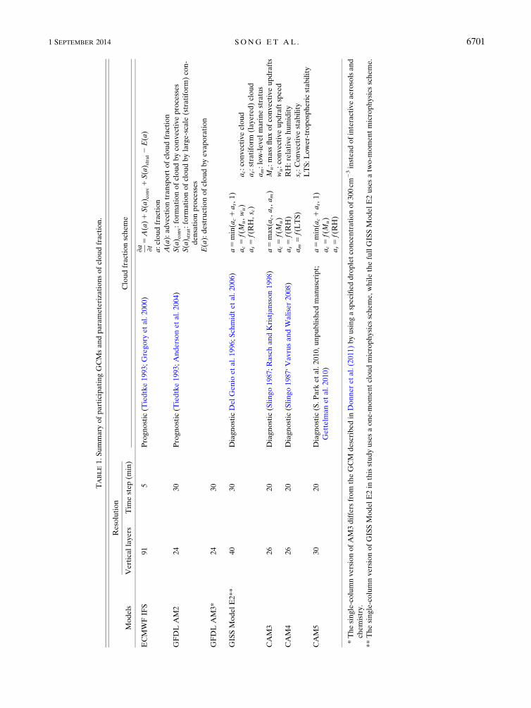
TABLE1.Summary

ofparticipatingGCMsandparameterizationsofcloudfraction.

Models

Resolution

Cloudfractionschem

eVerticallayers

Tim

estep(m

in)

ECMW

FIFS

91

5Prognostic(T

iedtke1993;Gregory

etal.2000)

›a ›t5A(a)1S(a) conv1S(a) strat2E(a)

a:cloudfraction

A(a):advectiontransport

ofcloudfraction

GFDLAM2

24

30

Prognostic(T

iedtke1993;Andersonetal.2004)

S(a) conv:form

ationofcloudbyconvectiveprocesses

S(a) strat:form

ationofcloudbylarge-scale

(stratiform

)con-

densationprocesses

E(a):destructionofcloudbyevaporation

GFDLAM3*

24

30

GISSModelE2**

40

30

Diagnostic

DelGenio

etal.1996;Schmidtetal.2006)

a5min(a

c1as,1)

ac5f(M

u,w

u)

ac:convectivecloud

as5f(RH,s c)

as:stratiform

(layered)cloud

am:low-levelmarinestratus

CAM3

26

20

Diagnostic

(Slingo1987;

RaschandKristjansson1998)

a5max(a

c,as,am)

Mu:mass

fluxofconvectiveupdrafts

ac5f(M

u)

wu:convectiveupdraftspeed

CAM4

26

20

Diagnostic

(Slingo1987‘

VavrusandW

aliser2008)

as5f(RH)

RH:relativehumidity

am5f(LTS)

s c:Convectivestability

LTS:Lower-troposphericstability

CAM5

30

20

Diagnostic

(S.Park

etal.2010,

unpublishedmanuscript;

Gettelm

anetal.2010)

a5min(a

c1as,1)

ac5f(M

u)

as5f(RH)

*Thesingle-columnversionofAM3differs

from

theGCM

describedin

Donner

etal.(2011)byusingaspecifieddropletconcentrationof300cm

23insteadofinteractiveaerosolsand

chemistry.

**Thesingle-columnversionofGISSModelE2in

thisstudyusesaone-m

omentcloudmicrophysics

schem

e,whilethefullGISSModelE2usesatw

o-m

omentmicrophysics

schem

e.

1 SEPTEMBER 2014 SONG ET AL . 6701

occurrence can represent large areal cloud fraction ob-

servations, which provides confidence for using the

ARSCLmultiyear cloud fraction to statistically evaluate

the simulated cloud fraction.

The ARMBE products also provide vertical profiles of

RH measured by balloon-borne soundings up to four

times daily at the ARM SGP Central Facility. The

sounding RH data have a known dry bias (Turner et al.

2003), but the ARMBEuses theMicrowave Radiometer-

Scaled Sonde Profiles (LSSONDE) value-added product

(VAP) to remove this bias (Turner et al. 1998; Xie et al.

2010). However, the sounding RH data are very sparse in

the years 1999–2001. There are only about 2400 h (about

300h at levels below 950hPa and above 150hPa) with

valid sounding RH, much less than the 25000h of valid

ARSCL cloud fraction and RUC-based RH in the con-

tinuous forcing dataset (Xie et al. 2004). Large differences

between the RUC-based RH and sounding RH are

shown to be mainly above 200-hPa level (Kennedy et al.

2011), where most sounding RH values are concentrated

at low RH ranges (RH , 5%) (Figs. S1 and S2 in the

supplementary material). Minnis et al. (2005) revealed

that the large differences between sounding RH and

RUC-based RH at high levels mainly occur in clear and

cloud-free conditions. In our simulations, we use the

RUC-based temperature and specific humidity from the

continuous forcing dataset to derive the relaxation terms

for temperature and specific humidity at each time step.

Considering all these factors, the RUC-based RH from

the continuous large-scale forcing dataset is used to

evaluate modeled RH as well.

The surface precipitation observational data used in

our analysis are the hourly Arkansas-Red Basin River

Forecast Center (ABRFC) 4-km rain gauge adjusted

Weather Surveillance Radar-1988 Doppler (WSR-88D)

measurements averaged over the variational analysis

domain (Xie et al. 2004).

3. Seasonal, diurnal, and vertical variations ofcloud fraction

The 3-yr average seasonal variations of cloud fraction

profile in the observations and seven SCMs are shown in

Fig. 1. The seasonal variations of the observed cloud

fraction exhibit a bimodal vertical distribution with

a higher peak at 400–200 hPa from January to July and

a lower peak around 850 hPa from March to June. The

largest cloud fraction occurs from winter to spring, when

baroclinic wave activities are common over the SGP site.

The minimum cloud fraction occurs during summer. The

three SCMs with prognostic cloud fraction schemes

(ECMWF IFS, GFDL AM2, and GFDL AM3) well

produce the seasonal variation pattern in the observations

(shading in Figs. 1b–d). For the other four SCMs with

diagnostic cloud fraction schemes, the GISS SCM cap-

tures the observed cloud fraction peaks in the cold season

(November–April) and cloud fraction minima in the

warm season (May–October), but all three CAM SCMs

have difficulty in capturing the observed seasonal phases

and generally have a weak seasonal contrast especially at

lower levels (shading in Figs. 1e–h).

Contours in Fig. 1 show the seasonal variations of cloud

fraction differences between the seven SCMs and obser-

vations. Compared with the observations, the ECMWF

SCM underestimates almost all clouds throughout the

year. The two GFDL SCMs underestimate low-level

clouds and overestimate high-level clouds in all months.

The GISS SCM underestimates clouds at most levels in

each month and mildly overestimates upper-level clouds

above 300hPa from October to April and lower-level

clouds between 600 and 800hPa in July and August. For

the three versions of CAM SCMs (SCAMs: SCAM3,

SCAM4, and SCAM5), there are some similarities and

differences. The SCAM4 has a similar bias pattern as the

SCAM3 but with smaller biases from May to November,

except for clouds around 200hPa and clouds below

800hPa from April to July. The SCAM3 and SCAM5

strongly overestimate upper-level cloud fraction between

350 and 200hPa, especially around May. Besides, the

SCAM5 has more near-surface low-level clouds than the

observations and other SCMs. One noteworthy point is

that, different from all the other SCMs, all three SCAMs

mildly overestimate lower-level cloud fraction during the

warm season. This feature is most likely a result of a day-

time bias in lower-level clouds in this season (not shown).

Here, daytime is defined as solar insolation at TOA being

larger than 0.01Wm22 (otherwise nighttime).

The striking phenomenon that only the three SCAMs

overestimate lower-level cloud fraction during warm

season deserves further inspection. Clouds in the three

SCAMs are composed of two types: convective and

stratiform, which are separately diagnosed and outputted

at each integration time step. Figure 2 shows the differ-

ences in monthly-mean daytime cloud fractions between

the convective clouds in the SCAMs and the total clouds

in the observations and that between the stratiform clouds

in the SCAMs and the total observed. It is striking that the

convective cloud fractions from the SCAMs alone are

already much larger than the observed total cloud frac-

tion in most months and at most levels, whereas the

stratiform clouds alone would have caused the un-

derestimation of lower-level cloud fraction (except below

850hPa for the SCAM5) and the overestimation of high-

level cloud fraction in most months in the three SCAMs.

These results imply that the overestimation of warm-

season lower-level clouds in the three SCAMs is mainly

6702 JOURNAL OF CL IMATE VOLUME 27

due to too many convective clouds that are diagnosed

from the convective mass flux. The excessive convective

cloud fraction in SCAMs ismainly due to their overactive

convection, which is easily triggered during the daytime

(Xie et al. 2002). It is also noteworthy that, during the

three years, events with nonzero convective cloud fraction

mainly occur during warm-season daytime at lower-to-

middle levels (Fig. 2, bottom),which leads to the negligible

FIG. 1. Seasonal variations of 3-yr monthly-mean cloud fraction in the (a) ARM observations and (b)–(h) seven

SCMs (shading) and model–observation differences in seasonal variations (contours). The contour interval is 4%.

1 SEPTEMBER 2014 SONG ET AL . 6703

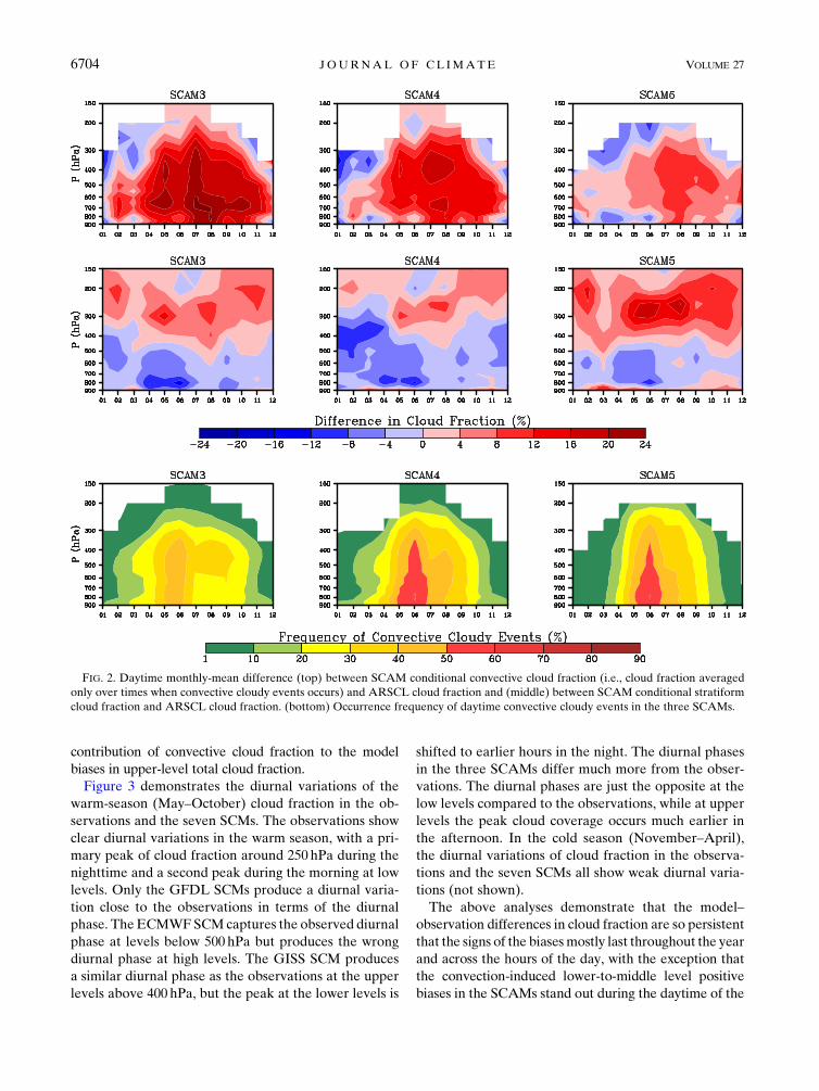
contribution of convective cloud fraction to the model

biases in upper-level total cloud fraction.

Figure 3 demonstrates the diurnal variations of the

warm-season (May–October) cloud fraction in the ob-

servations and the seven SCMs. The observations show

clear diurnal variations in the warm season, with a pri-

mary peak of cloud fraction around 250 hPa during the

nighttime and a second peak during the morning at low

levels. Only the GFDL SCMs produce a diurnal varia-

tion close to the observations in terms of the diurnal

phase. TheECMWFSCMcaptures the observed diurnal

phase at levels below 500 hPa but produces the wrong

diurnal phase at high levels. The GISS SCM produces

a similar diurnal phase as the observations at the upper

levels above 400 hPa, but the peak at the lower levels is

shifted to earlier hours in the night. The diurnal phases

in the three SCAMs differ much more from the obser-

vations. The diurnal phases are just the opposite at the

low levels compared to the observations, while at upper

levels the peak cloud coverage occurs much earlier in

the afternoon. In the cold season (November–April),

the diurnal variations of cloud fraction in the observa-

tions and the seven SCMs all show weak diurnal varia-

tions (not shown).

The above analyses demonstrate that the model–

observation differences in cloud fraction are so persistent

that the signs of the biasesmostly last throughout the year

and across the hours of the day, with the exception that

the convection-induced lower-to-middle level positive

biases in the SCAMs stand out during the daytime of the

FIG. 2. Daytime monthly-mean difference (top) between SCAM conditional convective cloud fraction (i.e., cloud fraction averaged

only over times when convective cloudy events occurs) and ARSCL cloud fraction and (middle) between SCAM conditional stratiform

cloud fraction and ARSCL cloud fraction. (bottom) Occurrence frequency of daytime convective cloudy events in the three SCAMs.

6704 JOURNAL OF CL IMATE VOLUME 27

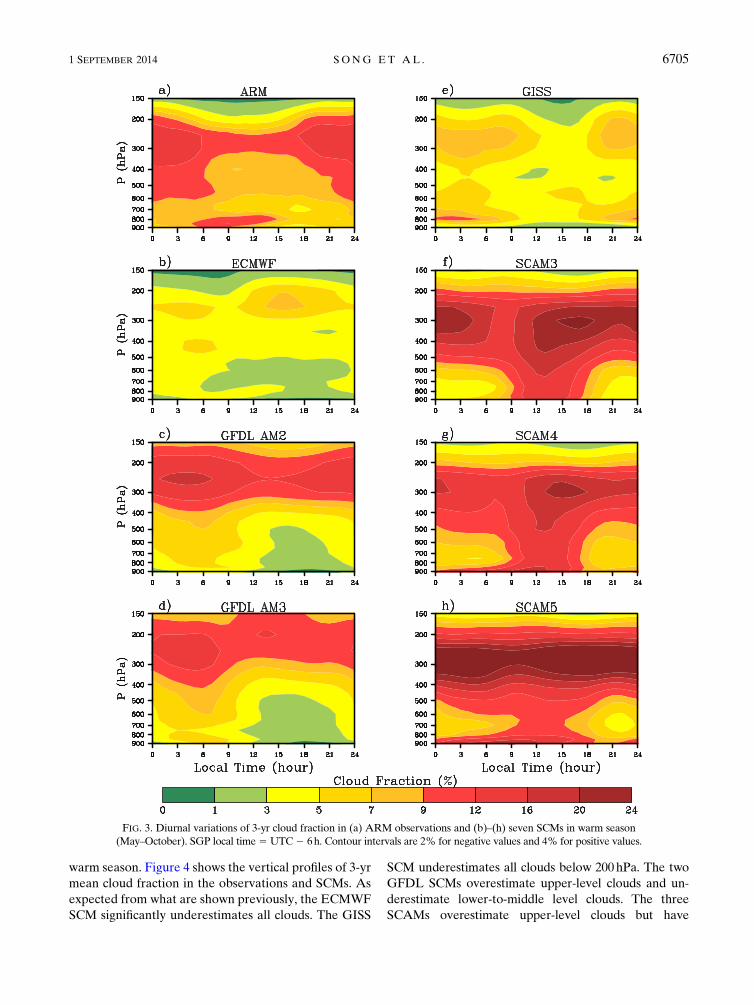
warm season. Figure 4 shows the vertical profiles of 3-yr

mean cloud fraction in the observations and SCMs. As

expected from what are shown previously, the ECMWF

SCM significantly underestimates all clouds. The GISS

SCM underestimates all clouds below 200hPa. The two

GFDL SCMs overestimate upper-level clouds and un-

derestimate lower-to-middle level clouds. The three

SCAMs overestimate upper-level clouds but have

FIG. 3. Diurnal variations of 3-yr cloud fraction in (a) ARM observations and (b)–(h) seven SCMs in warm season

(May–October). SGP local time5 UTC2 6h. Contour intervals are 2% for negative values and 4% for positive values.

1 SEPTEMBER 2014 SONG ET AL . 6705

a lower-level (800–600 hPa) cloud fraction similar to the

observations. However, a further inspection reveals that

the apparent agreement between the three SCAMs and

observations stems from the compensating over-

production of convective cloud fraction during the day-

time of the warm season and a general underproduction

of stratiform cloud fraction. The SCAM3 and SCAM5

both overestimate midlevel cloud fraction while the

SCAM4 underestimates. Besides, the SCAM5 has more

near-surface low-level clouds than the observations and

other SCMs. In short, compared with the observations,

most SCMs overestimate upper-level cloud fraction and

underestimate lower-level cloud fraction but still with

some differences in details. Note that here we loosely

define clouds above 350hPa as the upper-level clouds and

clouds below 600hPa as lower-level clouds to more

concisely characterize the discrepancies between the

observation and simulated cloud fraction from all the

seven SCMs. This partition is different from the con-

ventional definition (e.g., Hahn et al. 2001).

One source of errors in the cloud radar observations is

the attenuation during heavy precipitation events; the

radar tends to underestimate upper-level clouds when

precipitation is strong and the cloud is deep (Wu et al.

2009; Lin et al. 2012). To minimize the possible influence

of precipitation on the accuracy of the ARSCL cloud

fraction and thus the evaluation ofmodeled cloud fraction

against the observations, we excluded events with ob-

served surface precipitation rate larger than 40mmday21

in the following analyses. The model–observation cloud

fraction differences appear to have little dependence on

the observed precipitation rate when the observed pre-

cipitation rate is smaller than 40mmday21 (Fig. S3 in the

supplementary material). The total occurrence frequency

of heavy precipitation events (Pr. 40mmday21) is only

1.4% in the years from 1999 to 2001, and the vertical

profiles of 3-yr mean cloud fraction in the observations

and the seven SCMs after the exclusion of observed heavy

precipitation events are nearly identical to those in Fig. 4.

In the following sections, we investigate why the seven

SCMs have such striking biases in cloud fraction at dif-

ferent levels.

4. Partitioning analysis of cloud fraction

The preceding analysis shows that there are not only

significant differences between the SCMs and observa-

tions but also substantial intermodel discrepancies in the

simulated cloud fraction. The intermodel differences

can be due to their different stratiform and convective

cloud parameterizations. To identify the specific sources,

this section aims to partition the influences of these

two main types on the modeled cloud fraction.

In the diagnostic cloud fraction schemes of the GISS

Model E2 and three CAMs, the convective cloud frac-

tion and stratiform cloud fraction are calculated sepa-

rately. The convective cloud fraction is related to

updraft mass fluxes in the deep and shallow cumulus

schemes and the stratiform cloud fraction is a function of

RH and the threshold RH. In the prognostic cloud

fraction schemes of the ECMWFand twoGFDLGCMs,

the convection source term is proportional to the mass

detrainment of cumulus updrafts. The source term of the

stratiform process is a function of RH and only produces

cloud fraction when RH exceeds a threshold RH. The

evaporation term is also a function of RH. The strati-

form source term and evaporation sink term can be

considered together as the RH-related terms. Different

from the GISS and CAM models, the ECMWF and

GFDL models do not explicitly provide the contribu-

tions of stratiform source and convective source to total

cloud production. For consistency, a procedure com-

monly applicable to all the models is proposed and de-

scribed below that partitions cloud fraction into the

stratiform and nonstratiform (primarily convective)

cloud sources.

Because the detrainment rate and mass flux of deep/

shallow cumulus updrafts are not standard outputs of

most GCMs and were not saved for this study, we use

convective precipitation rate to indirectly represent

convection-related processes and define convective

events as the events whereby the modeled convective

precipitation rate is larger than 0.1mmday21. To further

FIG. 4. Vertical profiles of 3-yr mean cloud fraction in ARM

observations and seven SCMs.

6706 JOURNAL OF CL IMATE VOLUME 27

exclude the events with stratiform cloud production in

models during convective precipitation processes, we

also add an additional constraint of RH, 80% based on

the fact that thresholds of RH in the stratiform source

term in both prognostic and diagnostic schemes are

normally around 80% (from 60% to 90%) in most

models. Note that the variable thresholdRH in theGISS

model is about 60% on average; the analyses using RH

,80% or ,60% do not show any significant difference

for the GISS SCM.

For the ECMWF and GFDL SCMs using the prog-

nostic cloud fraction scheme, cloud fraction is locally

produced by the competition of the large-scale vertical

transport of cloud fraction, convection and/or large-

scale condensation processes, and evaporation, since the

continuous large-scale forcing data (Xie et al. 2004) do

not provide any large-scale hydrometeor advection.

Without horizontal advection of cloud fraction, clouds

cannot be removed from or added into the grid box by

surrounding dynamical fluxes. As a result, cloud fraction

in the next time step will keep on accumulating the

model bias at the previous time steps if there is no strong

source or sink of cloud fraction (hence small time ten-

dency of cloud fraction). Under such conditions, the

model cloud bias is not necessarily a flawed response of

model physics to the large-scale environment. To illus-

trate the influence of accumulated model bias in cloud

fraction on the following time step with weak time

tendency of cloud fraction, we also pick out the events

that have a small absolute value of modeled cloud

fraction tendency (much smaller than the cloud fraction

bias at the previous time step), convective precipitation

rate smaller than 0.1mmday21, and RH smaller than

80%. These events are neither purely convection nor

purely stratiform sources, and are included in the type of

nonstratiform-source events.

By use of the above partition procedure, modeled

cloudy events are separated into two types:

nonstratiform-source events (with convection sources or

small time tendency of cloud fraction for the ECMWF

and twoGFDL SCMs) and stratiform-source events. The

detailed criteria for the partitioning analysis are listed in

Table 2. It should be emphasized that this partitioning

method is tailored only for modeled cloud fraction. In the

real atmosphere the convective detrainment can produce

stratiform anvils, whereas in models these anvils may be

calculated from RH (when RH exceeds a threshold), in-

stead of by the convective scheme (e.g., in SCAMs).

Therefore, here we assume these anvil clouds in models

to be produced by the stratiform sources rather than the

convective sources (e.g., when convective precipitation

occurs and RH . 80%).

The 3-yr mean cloud fraction at each level can be

partitioned into the mean cloud fractions of the events

with nonstratiform sources and of the events with

stratiform sources, respectively,

CF5

�i5N

tot

i50

CFi

Ntot

5

�i5N

1

i50

CFijE1

Ntot

1

�i5N

2

i50

CFijE2

Ntot

1

�i5N

3

i50

CFijE3

Ntot

5CFnon-strat 1CFstrat 1CFboth , (1)

where CF stands for cloud fraction at any vertical level;

Ntot 5 25 852, which is the total number of time points

in the 3-yr hourly data; E1 represents nonstratiform-

source events; N1 is total number of time points with

nonstratiform-source events; E2 represents stratiform-

source events; N2 is total number of time points with

stratiform-source events; E3 represents events with

comparable nonstratiform source and stratiform source;

N3 is total number of time points with such events;Ntot5N1 1 N2 1 N3; CF represents the 3-yr mean cloud

fraction averaged for all events; CFnon-strat represents

the contribution of the nonstratiform-source events to

the 3-yr mean cloud fraction; CFstrat represents the

contribution of the stratiform-source events; and CFboth

represents the contribution of the events with compa-

rable nonstratiform source and stratiform source. Note

that, in the following analyses, we have not separately

considered the events with comparable nonstratiform

source and stratiform source because the contributions

of these events are very small in all SCMs. Instead we

include these events in the stratiform-source events.

The vertical profiles of 3-yr mean cloud fractions for

nonstratiform-source events and stratiform-source events

are illustrated in Fig. 5. It is seen that the contribution of

the nonstratiform-source events to the 3-yr mean cloud

fraction (Fig. 4) is mainly above the 600-hPa level in the

ECMWF and two GFDL SCMs and below the 400-hPa

level in three SCAMs. In the GISS SCM, the mean cloud

fraction of nonstratiform-source events is negligible and

less than 1%at all levels. ComparingFig. 5 with Fig. 4, the

overestimation of upper-level cloud fraction in the three

SCAMs can be clearly traced to the stratiform source,

while the overestimation of upper-level clouds in the

GFDL SCMs may be due to both stratiform and

1 SEPTEMBER 2014 SONG ET AL . 6707

nonstratiform sources. Similarly, the underestimation of

lower-level cloud fraction in the ECMWF SCM, two

GFDLSCMs, andGISS SCMmaybe due to lack of cloud

production by either or both the stratiform and non-

stratiform sources. Furthermore, the contribution of

stratiform-source events is much larger than that of

nonstratiform-source events at all levels in the tropo-

sphere (below 200 hPa) in all seven SCMs, indicating

the importance of stratiform (RH dependent) pro-

cesses in producing cloud fraction during the three

years (Fig. 4).

5. Frequency distribution of cloud fraction in theseven SCMs

Next we investigate the model performances over dif-

ferent cloud amount regimes. First we sort all the 3-yr

hourly cloud fraction data (total sample number is 25852)

by their amounts (from 0% to 100%) at each vertical

level, and then we calculate the occurrence frequencies of

cloud fraction at the specified ranges (each bin is 5%).

Here, frequency is the ratio of the number of events

within each specified cloud fraction range to the total

sample number. Figure 6 shows the frequency distri-

butions of cloud fraction over the cloud fraction ranges

from 0% to 100% at different vertical levels in the

seven SCMs. The most frequent events occur with

cloud fraction smaller than 10% at all levels in all

SCMs. Over the cloud fraction range from 10% to

100%, the frequency distributions are quite different

between the models with prognostic cloud fraction

schemes and those with diagnostic cloud fraction

schemes. Compared with the other SCMs, the ECMWF

SCM has much fewer occurrences of events with cloud

TABLE 2. Criteria used in the partitioning analysis. Stratiform-source events are all events excluding nonstratiform-source events. Note

that events with comparable nonstratiform source and stratiform source are not separately considered and are included in the stratiform-

source events.

Models Nonstratiform-source events at each time step t and vertical level p

ECMWF IFS Prconv(t). 0:1mmday21 and RH(t, p), 80%; or

GFDL AM2jaSCM(t2 1, p)2 aARM(t2 1, p)j.. jaSCM(t, p)2 aSCM(t2 1, p)j,Prconv(t), 0:1mmday21 and RH(t, p), 80%

� �GFDL AM3

GISS Model E2 Prconv(t). 0:1mmday21 and RH(t, p), 80%

CAM3

CAM4

CAM5

FIG. 5. (a) Vertical profiles of 3-yr mean cloud fraction in the seven SCMs for nonstratiform-source events. (b) Vertical

profiles of 3-yr mean cloud fraction in the ARM observations for all events and in the seven SCMs for stratiform-source

events. Events with observed surface precipitation rate larger than 40mmday21 are excluded.

6708 JOURNAL OF CL IMATE VOLUME 27

fraction larger than 40% at all levels (except for low-

level near-overcast events). The twoGFDL SCMs have

more high-level cloudy events than low-level cloudy

events over the cloudy range from 20% to 100%.

A special feature for the three SCAMs, different from

the models with prognostic cloud schemes, is the more

frequent occurrences of cloudy events over the range

from 10% to 50% at all levels. Besides, among the

FIG. 6. Frequency distributions of cloud fraction in seven SCMs binned by cloud fraction ranging from0% to 100%.

Each bin of cloud fraction is 5%. Events with observed surface precipitation rate larger than 40mmday21 are

excluded.

1 SEPTEMBER 2014 SONG ET AL . 6709

three SCAMs there are large discrepancies in the fre-

quency distributions. The SCAM4 has much fewer

occurrences of extensively cloudy events than the

SCAM3 and SCAM5. The SCAM5 has much more

frequent near-overcast events especially at high levels

than the SCAM3 and SCAM4.

Figure 7 presents the ratio of the nonstratiform-

source events to all the events for each total cloud

fraction bin in the seven SCMs. It is shown that, in the

SCMs with prognostic cloud scheme, especially in the

two GFDL SCMs, cloud fractions above the 400-hPa

level over the range 10%–80% are mainly produced

by the nonstratiform processes (contribution of the

events with small time tendency of cloud fraction is

about twice as large as that of the events with con-

vective sources), while cloud fractions below 700 hPa

are mainly produced by the stratiform processes. In

the GISS SCM, the cloudy events related to convec-

tion processes are rare, which is consistent with the

few convective precipitation events produced in the

GISS SCM (Song et al. 2013). Because of its parcel-

lifting-based trigger used in the convection scheme,

the GISS SCM cannot convect in most events when

the observation precipitation occurs (Del Genio and

Wolf 2012). Our precipitation study (Song et al. 2013)

shows that themean convective precipitation rates in both

the GISS and GFDL AM2 SCMs are very small but for

different reasons. In the GISS SCM both the occurrence

frequency and intensity of convective precipitation events

are very small, whereas in the GFDL AM2 SCM the in-

tensity of convective precipitation events is small but the

occurrence frequency of convective precipitation is high

and even higher than that in theGFDLAM3SCM.This is

also consistent with the overall higher ratio of nonstrati-

form events in the GFDL AM2 SCM than in the GFDL

AM3SCM, as can be seen in Fig. 7. For the three SCAMs,

their ratios of nonstratiform events suggest that the cloud

events below 400-hPa levels over the range 15%–50%

have a lot to do with the convective process, while the

cloud fractions below the 400-hPa level over the range

50%–100% and above the 300-hPa level over the whole

range are mainly produced by the stratiform process.

The diagnostic cloud fraction schemes calculate the

convective and stratiform cloud fractions separately, so

we can determine the relative roles of these two types of

cloud source in producing the total cloud fraction. Figure

8 illustrates the ratio of convective cloud fraction to total

cloud fraction averaged over each cloud fraction bin in the

GISS SCMand the three SCAMs. The distributions of the

ratios are generally similar to those in Fig. 7 for the GISS

SCM and SCAMs. This confirms the reliability of using

convective precipitation rate and RH , 80% to choose

the convective events for thesemodels. In theGISS SCM,

the ratio of convective cloud fraction to total cloud frac-

tion averaged over each bin of total cloud amount is very

small. The very small convective cloud fraction in the

GISS SCMsimulation is also reported inKennedy (2011).

In the three SCAMs, over the range from 15% to 50%,

clouds below the 400-hPa level have a large contribution

from convective sources. Together, the results in Figs. 6–8

suggest that the diagnostic schemes related to the con-

vective processes in the three SCAMs produce too many

clouds over this range too frequently. It is also seen in Fig.

8 that, over the range from 60% to 100%, cloud fractions

are mainly contributed by stratiform (nonconvective)

clouds, which is diagnosed fromRHwith a threshold RH.

6. Cloud fraction and RH

Many previous studies have shown the strong re-

lationship between cloud fraction and RH in the obser-

vations and models (e.g., Slingo 1980; Xu and Randall

1996a,b). For stratiform cloud fraction in models, there

are three ways in which RH could possibly influence the

calculation of cloud amount: 1) values of threshold RH

used in the cloud scheme; 2) dependence of cloud fraction

on RH above the threshold (viz., the diagnostic formula);

and 3)modeledRH. The frequency distribution of cloudy

events is mainly related to ways 1 and 3, whereas the

mean cloud amount is mainly related to ways 2 and 3.

Note that in this study, RH is defined with respect to

liquid and/or ice depending on air temperature. Satura-

tion mixing ratio with respect to liquid (ice) is used when

temperature is above 08C (below 2208C), and a linear

combination with respect to liquid and ice is used be-

tween 08 and 2208C. Next we dissect these possible in-

fluences of RH on the model biases in cloud fraction,

revealing a close link to model parameterizations.

a. Diagnosis of the threshold RH

As discussed above, cloud fraction in all the seven

models is related to a threshold RH, which is specified in

some models but a variable in others. Quaas (2012) pro-

posed an approach to estimate the threshold RH from

cloud fraction and RH in both observations and models

and demonstrated that the threshold RH value is a pow-

erful diagnostic for evaluating the representation of

subgrid variability in cloud fraction parameterizations in

GCMs. Low values of the threshold RH indicate large

subgrid-scale variability of humidity. It is noteworthy

that the threshold RH diagnosed here is a common

measure for purpose of comparison, not the exact

threshold RH used in the cloud fraction schemes.

Briefly, assuming a uniform probability density func-

tion (PDF) of total water specific humidity qt in the grid

box and that clouds only occur in the area where qt is

6710 JOURNAL OF CL IMATE VOLUME 27

larger than saturation specific humidity qs, the uniform

PDF with a width related to qs can be formulated in

terms of threshold RH rc, and then cloud fraction f can

be expressed in terms of the gridbox mean RH r and rc(Sundqvist et al. 1989),

f 5 12

12 r

12 rc

!1/2

, (2)

where f 5 0 for r# rc and f 5 1 for r$ 1.

FIG. 7. Ratios of nonstratiform-source events to all the events for each total cloud fraction bins (each bin is 5%) in the

seven SCMs. Events with observed surface precipitation rate larger than 40mmday21 are excluded.

1 SEPTEMBER 2014 SONG ET AL . 6711

Using cloud fraction and RH from the models or ob-

servations, the threshold RH can be calculated

(0, f , 1),

rc5 1212 r

(12 f )2. (3)

Figure 9a shows the vertical profiles of the 3-yr mean

threshold RH in the observations and the seven SCMs.

Here the hourly RUC-based RH and hourly ARSCL

cloud fraction are used to calculate the hourly threshold

RH in the observations. It is seen that, compared with

the observations, at levels below 400 hPa all seven SCMs

(except the GISS SCM at certain levels) have larger

threshold RH, while at levels above 400 hPa the two

GFDL SCMs have smaller threshold RH and the

ECMWF SCM and the three SCAMs still have larger

threshold RH. The larger threshold RH in most SCMs

also indicates their smaller subgrid variability of RH

than the observations. The diagnosed threshold RH

in Fig. 9a does not distinguish clouds of stratiform or

nonstratiform. The nonstratiform clouds in the models

are presumably produced by the convective schemes.

Although the calculation of such clouds does not di-

rectly involve RH, practically what constitutes the

overall threshold RHs in Fig. 9a can be separated into

those associated with stratiform and nonstratiform

clouds. The vertical profiles of the diagnosed threshold

RH for nonstratiform and stratiform events in the seven

SCMs are shown in Fig. 9b. The values of threshold RH

in the stratiform events aremuch larger than those in the

nonstratiform events. This again implies that cumulus

parameterizations do not use RH directly to form clouds

(except to the extent that high PBL RH is needed for

CAPE or buoyancy) and that such clouds often occur

when the grid box as a whole, at least above the

boundary layer, is drier than that needed to form strat-

iform clouds. It is also shown that the larger threshold

RH values in most models (Fig. 9a) are mainly con-

tributed by the threshold RHs of stratiform events,

whereas the smaller threshold RH values in the GFDL

SCMs at upper levels (Fig. 9a) are because of the higher

ratio of nonstratiform events and the associated smaller

threshold RH.

b. Dependence of cloud fraction on RH

The vertical profiles ofmean cloud fraction binned byRH

in the observations and seven SCMs are shown in Fig. 10

(shading). Note the RUC-based RH is used as the ob-

servation for the reasons discussed in section 2b. Cloud

fraction increases with RH in both the observations and

seven SCMs but more sharply at high RH ranges in most

SCMs. Also, themodel–observation differences in mean

FIG. 8. Averaged ratios of the convective cloud fraction to total

cloud fraction for each total cloud fraction bins (each bin is 5%) in the

GISS SCM and three SCAMs. Events with observed surface pre-

cipitation rate larger than 40mmday21 are excluded.

6712 JOURNAL OF CL IMATE VOLUME 27

cloud fraction binned by RH (contours in Fig. 10) show

large differences in the distribution patterns. In both

the ECMWF andGISS SCMs, the mean cloud fractions

at each RH bin are much smaller than the observations

at most levels, which can be partly attributed to the

weak dependence of cloud fraction on RH in these two

models and generally larger RH threshold for strati-

form clouds as shown in Fig. 9. Lack of nonstratiform

cloud source at small cloud fractions in the GISS SCM

(Fig. 7) also makes it unable to mitigate the negative

biases. In the twoGFDL SCMs at levels below 300 hPa,

the mean cloud fractions are much smaller than the

observations at most RH ranges, while at levels above

300 hPa the mean cloud fractions are larger than the

observations at all RH ranges, especially at the high

RH ranges. In the three SCAMs, at lower levels mean

cloud fractions at low RH ranges are slightly larger

than observed. The positive cloud biases in GFDL and

CAM SCMs at low-to-moderate RH ranges are most

likely due to their excessive nonstratiform cloud pro-

duction, while the negative biases at these low-to-

moderate RH ranges may be primarily attributable to

the requirement of higher RH threshold for stratiform

clouds. Figure 11 shows the frequency distributions of

RUC-based RH and modeled RH for each RH bins. It

is seen that the distribution of RH favors low RH

(10%–40%) at lower-to-middle levels much more than

at the upper levels. The ECMWF, two GFDL, and

GISS SCMs have similar frequency distributions as that

of the RUC-based RH, mainly with differences smaller

than 1%.However, the three SCAMs have significantly

different frequency distributions of RH from those of

the RUC-based RH (contours in Fig. 11) and other

SCMs. There is a much higher frequency of large RH

and a lower frequency of small RH, especially at levels

above 500 hPa, in three SCAMs, indicating the strong

overestimation of high-level RH. Combining the

model–observation differences in mean cloud fraction

and differences in RH distribution, it can be seen that

the cause of upper-level cloud fraction in the seven

SCMs differs substantially. In the ECMWF and GISS

SCMs, the underestimation of upper-level cloud frac-

tion may be primarily due to their weaker relationship

between cloud fraction and RH. In the two GFDL

SCMs, the overestimations of upper-level cloud frac-

tion are mainly due to larger mean cloud fraction of

cloudy events and more events, with RH ranging from

40% to 80% (Fig. S5 in the supplementary material). In

the three SCAMs, the overestimation of upper-level

cloud fraction is mainly due to the strong over-

estimation of RH. While the overestimation of lower-

level clouds in SCAMs can be attributed to excessive

convective cloud production, the underestimation of

lower-level cloud fraction in the rest of SCMs may be

primarily attributed to the fact that most events in the

three years have RH smaller than threshold RH and

models have larger threshold RH than the observations

(Fig. 9).

It is noteworthy that we have also found that the re-

lationship between cloud fraction and RH varies with

FIG. 9. (a) Vertical profiles of the diagnosed threshold RH in the observations and seven SCMs. (b) Vertical

profiles of thresholdRH in theARMobservations (black solid line) and seven SCMs for nonstratiform-source events

(dashed–dotted lines) and for stratiform-source events (dashed lines). Events with observed surface precipitation

rate larger than 40mmday21 are excluded. The RUC-based RH data are used to derive threshold RH in the

observations.

1 SEPTEMBER 2014 SONG ET AL . 6713

FIG. 10. Vertical profiles of mean cloud fraction in the ARM observations binned by the RUC-based RH and in

seven SCMs binned by modeled RH (shading) and cloud fraction differences between the observations and seven

SCMs (contours). Each bin of RH is 5%.

6714 JOURNAL OF CL IMATE VOLUME 27

seasons in both observations and seven SCMs, with

a tighter correlation in cold seasons when stratiform

cloudy events dominate (Fig. S4 in the supplementary

material). Meanwhile, cloud fraction has a much

stronger relationship with RH in most SCMs than in the

observations, which may be partially due to the fact that

the RUC-based RH are not always well matched to the

ARSCL point observations.

FIG. 11. As in Fig. 10, but for frequency of RH in the RUC-based forcing and seven SCMs. Events with observed

surface precipitation rate larger than 40mmday21 are excluded.

1 SEPTEMBER 2014 SONG ET AL . 6715

7. Summary

This study quantitatively evaluates the overall per-

formances of seven SCMs by comparing simulated cloud

fraction with the observations at the ARM SGP site.

Striking differences in cloud fraction are found not only

between the SCMs and the observations but also among

the SCMs themselves, in terms of mean cloud fraction

and frequency distribution.

The seasonal and diurnal variation analyses demon-

strate that the model–observation differences in cloud

fraction are so persistent that the signs of the biases

mostly last throughout the year and across the hours of

the day, with the exception that the convection-induced

lower-level positive biases in the SCAMs stand out

during the daytime of the warm season. Compared with

the 3-yr mean ARSCL cloud fraction, most of the

SCMs overestimate upper-level cloud fraction and un-

derestimate lower-level cloud fraction but still with

some differences in details. The ECMWF SCM un-

derestimates cloud fraction at all levels, and the GISS

SCM underestimates cloud fraction at levels below

200hPa. The GFDL SCMs underestimate lower-to-

middle-level cloud fraction but overestimate upper-level

cloud fraction. The SCAMs overestimate upper-level

cloud fraction and produce lower-level cloud fraction

(600–800hPa) similar to the observations. The SCAM3

and SCAM5 both overestimate midlevel cloud fraction

while the SCAM4 underestimates. Also, the SCAM5 has

more near-surface lower-level clouds than the observa-

tions and other SCMs.

The frequency distribution of cloud fraction shows

a large discrepancy among the seven SCMs, especially

between models with prognostic cloud fraction schemes

and those with diagnostic cloud fraction schemes. Par-

titioning analysis further shows that the contribution of

the stratiform process is much larger than that of the

nonstratiform process to 3-yr mean cloud fraction at all

levels below 200 hPa in all seven SCMs, indicating the

importance of the stratiform process in producing cloud

fraction in models. Despite a smaller contribution to

the total cloud fraction, nonstratiform processes for

cloud fraction production at different vertical levels

and cloud fraction ranges are quite different among the

seven SCMs. This large intermodel difference in non-

stratiform processes seems consistent with that in con-

vection parameterization and precipitation as reported

in Song et al. (2013). Further analysis reveals different

relationships between cloud fraction and RH in the

models and observations. The consistent lower-level RH

distribution in the SCMs and observations implies that

the underestimation of lower-level cloud fraction in

most SCMs is mainly due to the larger threshold RH

used in the models, while biases in the upper-level cloud

fraction for different SCMs exist for quite different

reasons. Analysis of threshold RH suggests that there

are substantial differences in the representation of

subgrid variability among the seven models, and be-

tween the models and the observations. This finding

reinforces the increasing recognition of the need for

improving the representation of subgrid variability in

climate models (Tompkins 2002; Wood and Hartmann

2006).

Compared to the precipitation performance reported

in Song et al. (2013), the results show that unlike pre-

cipitation, the cloud fraction biases of the seven SCMs

(stratiform cloud fraction for three SCAMs) are quite

consistent during different seasons, daytime or night-

time. This is most likely related to the fact that, at the

SGP site, the mean precipitation is dominated by con-

vective precipitation whereas the mean cloud fraction is

dominated by stratiform cloud fraction.

A few points are noteworthy. First, the continuous

large-scale forcing used in our SCM simulations has

some well-known limitations. For example, Kennedy

et al. (2011) showed that the continuous forcing data

have a moist bias in the boundary layer and at the

upper levels, especially above 200 hPa, when com-

pared to the ARMBE soundings (Fig. S1). This moist

bias at the boundary layer likely influences the model

convection process, especially for SCMs with CAPE-

based triggers. Another deficiency is the lack of large-

scale hydrometeor advection in the continuous forcing

data, which can influence modeled cloud fraction

and precipitation through the prognostic cloud frac-

tion scheme and/or prognostic cloud microphysical

schemes. To further address possible influences of

the forcing data on our SCM performances, simula-

tions with an ensemble of long-term forcings will be

carried out when different forcing data become

available. Second, analysis of RH threshold in this

study reveals some problems with the cloud fraction

representation in climate models (e.g., RH represen-

tation and subgrid variability). Higher-resolution

models such as cloud-resolving model or large-eddy

simulations (e.g., Xu and Randall 1996b; Siebesma

et al. 2003; Cheng and Xu 2011) can be used for further

improving cloud parameterizations in GCMs. Finally,

similar biases of cloud fraction identified in the seven

SCMs at the SGP site can also be seen in some of their

parent global models and many other GCMs (Qian

et al. 2012; Fig. S6 in the supplementary material).

Current cloud fraction schemes in models cannot well

reproduce the observed cloud fraction (e.g., Xu and

Randall 1996a; Lauer and Hamilton 2013). A better

and more physically based cloud fraction scheme is

6716 JOURNAL OF CL IMATE VOLUME 27

needed to ultimately remove the deficiencies in cli-

mate models.

Acknowledgments. This work is supported by the

Office of Biological and Environmental Research of the

U.S. Department of Energy as part of the Earth Systems

Modeling (ESM) program via the FASTER project

(http://www.bnl.gov/faster) and Atmospheric System

Research program. Del Genio is supported also by the

NASA Modeling and Analysis Program. We thank

Editor Dr. Robert Wood and three anonymous re-

viewers for their insightful and constructive comments.

We also thank Dr. Stephen Schwartz for his interest and

helpful suggestions.

REFERENCES

Ackerman, T. P., and G. M. Stokes, 2003: The Atmospheric Ra-

diation Measurement Program. Phys. Today, 56, 38–44,

doi:10.1063/1.1554135.

Anderson, J., andCoauthors, 2004: The newGFDLglobal atmosphere

and land model AM2–LM2: Evaluation with prescribed SST

simulations. J. Climate, 17, 4641–4673, doi:10.1175/JCLI-3223.1.

Boucher, O., and Coauthors, 2014: Clouds and aerosols. Climate

Change 2013: The Physical Science Basis, T. F. Stocker et al.,

Eds., Cambridge University Press, 571–657.

Bretherton, C. S., J. R. McCaa, and H. Grenier, 2004: A new pa-

rameterization for shallow cumulus convection and its appli-

cation tomarine subtropical cloud-toppedboundary layers. Part

I: Description and 1D results. Mon. Wea. Rev., 132, 864–882,

doi:10.1175/1520-0493(2004)132,0864:ANPFSC.2.0.CO;2.

Cess, R. D., and Coauthors, 1996: Cloud feedback in atmospheric

general circulation models: An update. J. Geophys. Res., 101,

12 791–12 794, doi:10.1029/96JD00822.

Cheng, A., and K.-M. Xu, 2011: Improved low-cloud simulation

from a multiscale modeling framework with a third-order

turbulence closure in its cloud-resolving model component.

J. Geophys. Res., 116, D14101, doi:10.1029/2010JD015362.

Clothiaux, E. E., and Coauthors, 1999: The Atmospheric Radia-

tion Measurement Program cloud radars: Operational

modes. J. Atmos. Oceanic Technol., 16, 819–827, doi:10.1175/

1520-0426(1999)016,0819:TARMPC.2.0.CO;2.

——, T. P. Ackerman, G. G. Mace, K. P. Moran, R. T. Marchand,

M. A.Miller, and B. E. Martner, 2000: Objective determination

of cloud heights and radar reflectivities using a combination of

active remote sensors at the ARM CART sites. J. Appl. Me-

teor., 39, 645–665, doi:10.1175/1520-0450(2000)039,0645:

ODOCHA.2.0.CO;2.

Davies, L., and Coauthors, 2013: A single-column model ensemble

approach applied to the TWP-ICE experiment. J. Geophys.

Res., 118, 6544–6563, doi:10.1002/jgrd.50450.

Del Genio, A. D., and A. Wolf, 2012: Should today’s SCMs

convect at the SGP? ASR Science Team Meeting, Arlington,

VA, U.S. Department of Energy, 11 pp. [Available online at

http://asr.science.energy.gov/meetings/stm/2012/presentations/

delgeniofaster.pdf.]

——, M.-S. Yao, W. Kovari, and K. K.-W. Lo, 1996: A prognostic

cloud water parameterization for global climate models.

J. Climate, 9, 270–304, doi:10.1175/1520-0442(1996)009,0270:

APCWPF.2.0.CO;2.

——,A. B.Wolf, andM. S. Yao, 2005: Evaluation of regional cloud

feedbacks using single-column models. J. Geophys. Res., 110,

D15S13, doi:10.1029/2004JD005011.

Dong, X., B. Xi, and P. Minnis, 2006: A climatology of midlatitude

continental clouds from the ARM SGP Central Facility. Part

II: Cloud fraction and surface radiative forcing. J. Climate, 19,

1765–1783, doi:10.1175/JCLI3710.1.

Donner, L. J., C. J. Seman, R. S. Hemiler, and S. Fan, 2001:

A cumulus parameterization including mass fluxes, convective

vertical velocities, and mesoscale effects: Thermodynamic

and hydrological aspects in a general circulation model.

J. Climate, 14, 3444–3463, doi:10.1175/1520-0442(2001)014,3444:

ACPIMF.2.0.CO;2.

——, and Coauthors, 2011: The dynamical core, physical parame-

terizations, and basic simulation characteristics of the atmo-

spheric component AM3 of the GFDL global coupled model

CM3. J. Climate, 24, 3484–3519, doi:10.1175/2011JCLI3955.1.Gettelman, A., and Coauthors, 2010: Global simulations of ice

nucleation and ice supersaturation with an improved cloud

scheme in the Community Atmosphere Model. J. Geophys.

Res., 115, D18216, doi:10.1029/2009JD013797.

GEWEX Cloud System Science Team, 1993: The GEWEX Cloud

System Study. Bull. Amer. Meteor. Soc., 74, 387–400,

doi:10.1175/1520-0477(1993)074,0387:TGCSS.2.0.CO;2.

Ghan, S., and Coauthors, 2000: An intercomparison of single col-

umn model simulations of summertime midlatitude conti-

nental convection. J. Geophys. Res., 105, 2091–2124,

doi:10.1029/1999JD900971.

Gregory, D., J. J. Morcrette, C. Jakob, A. C. M. Beljaars, and

T. Stockdale, 2000: Revision of convection, radiation and

cloud schemes in the ECMWF Integrated Forecasting System.

Quart. J. Roy. Meteor. Soc., 126, 1685–1710, doi:10.1002/

qj.49712656607.

Hahn, C. J., W. B. Rossow, and S. G. Warren, 2001: ISCCP cloud

properties associated with standard cloud types identified in

individual surface observations. J. Climate, 14, 11–28,

doi:10.1175/1520-0442(2001)014,0011:ICPAWS.2.0.CO;2.

Henderson, P. W., and R. Pincus, 2009: Multiyear evaluations of

a cloud model using ARM data. J. Atmos. Sci., 66, 2925–2936,

doi:10.1175/2009JAS2957.1.

Kennedy, A. D., 2011: Evaluation of a single column model at the

Southern Great Plains Climate Research Facility. Ph. D. dis-

sertation, University of North Dakota, 149 pp.

——, X. Dong, B. Xi, P. Minnis, A. D. Del Genio, A. B. Wolf, and

M. M. Khaiyer, 2010: Evaluation of the NASA GISS Single-

Column Model simulated clouds using combined surface and

satellite observations. J. Climate, 23, 5175–5192, doi:10.1175/

2010JCLI3353.1.

——, ——, ——, S. Xie, Y. Zhang, and J. Chen, 2011: A compar-

ison ofMERRAandNARR reanalysis datasets with theDOE

ARM SGP continuous forcing data. J. Climate, 24, 4541–4557,

doi:10.1175/2011JCLI3978.1.

Klein, S. A., and D. L. Hartmann, 1993: The seasonal cycle of

low stratiform clouds. J. Climate, 6, 1587–1606, doi:10.1175/

1520-0442(1993)006,1587:TSCOLS.2.0.CO;2.

——, and Coauthors, 2009: Intercomparison of model simulations

of mixed-phase clouds observed during the ARM Mixed-

Phase Arctic Cloud Experiment. I: Single-layer cloud. Quart.

J. Roy. Meteor. Soc., 135, 979–1002, doi:10.1002/qj.416.

Lauer, A., and K. Hamilton, 2013: Simulating clouds with global

climate models: A comparison of CMIP5 results with CMIP3

and satellite data. J. Climate, 26, 3823–3845, doi:10.1175/

JCLI-D-12-00451.1.

1 SEPTEMBER 2014 SONG ET AL . 6717

Lin, Y., and Coauthors, 2012: TWP-ICE global atmospheric model

intercomparison: Convection responsiveness and resolution im-

pact. J. Geophys. Res., 117, D09111, doi:10.1029/2011JD017018.

Minnis, P., Y. Yi, J. Huang, and K. Ayers, 2005: Relationships

between radiosonde and RUC-2 meteorological conditions

and cloud occurrence determined from ARM data. J. Geo-

phys. Res., 110, D23204, doi:10.1029/2005JD006005.

Moorthi, S., and M. J. Suarez, 1992: Relaxed Arakawa-Schubert:

A parameterization of moist convection for general circula-

tion models. Mon. Wea. Rev., 120, 978–1002, doi:10.1175/

1520-0493(1992)120,0978:RASAPO.2.0.CO;2.

Morrison, H., and Coauthors, 2009: Intercomparison of model

simulations of mixed-phase clouds observed during the ARM

Mixed-Phase Arctic Cloud Experiment. II: Multilayer cloud.

Quart. J. Roy. Meteor. Soc., 135, 1003–1019, doi:10.1002/

qj.415.

Naud, C. M., A. D. Del Genio, M. Bauer, and W. Kovari, 2010:

Cloud vertical distribution across warm and cold fronts in

CloudSat–CALIPSO data and a general circulation model.

J. Climate, 23, 3397–3415, doi:10.1175/2010JCLI3282.1.

Neggers, R. A. J., A. P. Siebesma, and T. Heus, 2012: Continuous

single-column model evaluation at a permanent meteorolog-

ical supersite. Bull. Amer. Meteor. Soc., 93, 1389–1400,

doi:10.1175/BAMS-D-11-00162.1.

Qian, Y., C. N. Long, H. Wang, J. M. Comstock, S. A. McFarlane,

and S. Xie, 2012: Evaluation of cloud fraction and its radiative

effect simulated by IPCC AR4 global models against ARM

surface observations. Atmos. Chem. Phys., 12, 1785–1810,

doi:10.5194/acp-12-1785-2012.

Quaas, J., 2012: Evaluating the ‘‘critical relative humidity’’ as

a measure of subgrid-scale variability of humidity in general

circulation model cloud cover parameterizations using satel-

lite data. J. Geophys. Res., 117, D09208, doi:10.1029/

2012JD017495.

Randall, D. A., and D. G. Cripe, 1999: Alternative methods for

specification of observed forcing in single-column models and

cloud system models. J. Geophys. Res., 104, 24 527–24 545,

doi:10.1029/1999JD900765.

——, K.-M. Xu, R. J. C. Somerville, and S. Iacobellis, 1996: Single-

column models and cloud ensemble models as links between

observations and climate models. J. Climate, 9, 1683–1697,

doi:10.1175/1520-0442(1996)009,1683:SCMACE.2.0.CO;2.

Rasch, P. J., and J. E. Kristjansson, 1998: A comparison of the

CCM3 model climate using diagnosed and predicted con-

densate parameterizations. J. Climate, 11, 1587–1614,

doi:10.1175/1520-0442(1998)011,1587:ACOTCM.2.0.CO;2.

Schmidt, G. A., and Coauthors, 2006: Present-day atmospheric

simulations using GISS ModelE: Comparison to in situ, sat-

ellite, and reanalysis data. J. Climate, 19, 153–192, doi:10.1175/

JCLI3612.1.

Siebesma, A. P., and Coauthors, 2003: A large eddy simulation

intercomparison study of shallow cumulus convection. J. At-

mos. Sci., 60, 1201–1219, doi:10.1175/1520-0469(2003)60,1201:

ALESIS.2.0.CO;2.

Slingo, J. M., 1987: The development and verification of a cloud

prediction scheme for the ECMWF model. Quart. J. Roy.

Meteor. Soc., 113, 899–927, doi:10.1002/qj.49711347710.

——, 1980: A cloud parameterization scheme derived fromGATE

data for use with a numerical model. Quart. J. Roy. Meteor.

Soc., 106, 747–770, doi:10.1002/qj.49710645008.Solomon, S., D. Qin,M.Manning, Z. Chen,M.Marquis, K. Averyt,

M. Tignor, and H. L. Miller Jr., Eds., 2007: Climate Change

2007: The Physical Science Basis.CambridgeUniversity Press,

996 pp.

Song, H., W. Lin, Y. Lin, A. B.Wolf, R. Neggers, L. J. Donner, A. D.

Del Genio, and Y. Liu, 2013: Evaluation of precipitation

simulated by seven SCMs against the ARM observations at the

SGPsite. J.Climate, 26,5467–5492, doi:10.1175/JCLI-D-12-00263.1.

Stephens, G. L., and Coauthors, 2002: The CloudSat mission and

the A-Train. Bull. Amer. Meteor. Soc., 83, 1771–1790,

doi:10.1175/BAMS-83-12-1771.

Stokes, G.M., and S. E. Schwartz, 1994: TheAtmospheric Radiation

Measurement (ARM) program: Programmatic background and

design of the cloud and radiation test bed. Bull. Amer. Meteor.

Soc., 75, 1202–1221, doi:10.1175/1520-0477(1994)075,1201:

TARMPP.2.0.CO;2.

Sundqvist, H., E. Berge, and J. E. Kristjánsson, 1989: Conden-sation and cloud parameterization studies with a meso-

scale numerical weather prediction model.Mon. Wea. Rev.,

117, 1641–1657, doi:10.1175/1520-0493(1989)117,1641:

CACPSW.2.0.CO;2.

Tiedtke,M., 1993: Representation of clouds in large-scalemodels.Mon.

Wea. Rev., 121, 3040–3061, doi:10.1175/1520-0493(1993)121,3040:

ROCILS.2.0.CO;2.

Tompkins,A.M., 2002:Aprognostic parameterization for the subgrid-

scale variability of water vapor and clouds in large-scale models

and its use to diagnose cloud cover. J. Atmos. Sci., 59, 1917–1942,

doi:10.1175/1520-0469(2002)059,1917:APPFTS.2.0.CO;2.

——, K. Gierens, and G. Rädel, 2007: Ice supersaturation in the

ECMWF integrated forecast system. Quart. J. Roy. Meteor.

Soc., 133, 53–63, doi:10.1002/qj.14.

Turner, D. D., T. R. Shippert, P. D. Brown, S. A. Clough, R. O.

Knuteson, H. E. Revercomb, and W. L. Smith, 1998: Long-

term analyses of observed and line-by-line calculations of

longwave surface spectral radiance and the effect of scaling

the water vapor profile. Proc. Eighth Atmospheric Radiation

Measurement Science Team Meeting, Tucson, AZ, U.S. De-

partment of Energy, 773–776.

——, B. M. Lesht, S. A. Clough, J. C. Liljegren, H. E. Revercomb,

andD.C. Tobin, 2003: Dry bias and variability inVaisalaRS80-

H radiosondes: The ARM experience. J. Atmos. Oceanic

Technol., 20, 117–132, doi:10.1175/1520-0426(2003)020,0117:

DBAVIV.2.0.CO;2.

Vavrus, S., and D. Waliser, 2008: An improved parameteriza-

tion for simulating Arctic cloud amount in the CCSM3

climate model. J. Climate, 21, 5673–5687, doi:10.1175/

2008JCLI2299.1.

Wood, R., and D. L. Hartmann, 2006: Spatial variability of liquid

water path in marine low cloud: The importance of mesoscale

cellular convection. J. Climate, 19, 1748–1764, doi:10.1175/

JCLI3702.1.

Wu, J., A. D. Del Genio, M.-S. Yao, and A. B. Wolf, 2009: WRF

and GISS SCM simulations of convective updraft properties

during TWP-ICE. J. Geophys. Res., 114,D04206, doi:10.1029/

2008JD010851.

Xie, S., and Coauthors, 2002: Intercomparison and evaluation of

cumulus parameterizations under summertime midlatitude

continental conditions.Quart. J. Roy. Meteor. Soc., 128, 1095–

1135, doi:10.1256/003590002320373229.

——, R. T. Cederwall, and M. Zhang, 2004: Developing long-term

single-column model/cloud system-resolving model forcing

data using numerical weather prediction products constrained

by surface and top of atmosphere observations. J. Geophys.

Res., 109, D01104, doi:10.1029/2003JD004045.

6718 JOURNAL OF CL IMATE VOLUME 27

——, and Coauthors, 2005: Simulations of midlatitude frontal

clouds by single-column and cloud-resolving models during

the Atmospheric Radiation Measurement March 2000 cloud

intensive operational period. J. Geophys. Res., 110, D15S03,

doi:10.1029/2004JD005119.

——, and Coauthors, 2010: Cloud and more: ARM climate mod-

eling best estimate data. Bull. Amer. Meteor. Soc., 91, 13–20,

doi:10.1175/2009BAMS2891.1.

Xu, K.-M., and S. K. Krueger, 1991: Evaluation of cloudiness pa-

rameterizations using a cumulus ensemble model. Mon. Wea.

Rev., 119, 342–367, doi:10.1175/1520-0493(1991)119,0342:

EOCPUA.2.0.CO;2.

——, and D. A. Randall, 1996a: Evaluation of statistically based

cloudiness parameterizations used in climate models. J. Atmos.

Sci., 53, 3103–3119, doi:10.1175/1520-0469(1996)053,3103:

EOSBCP.2.0.CO;2.

——, and ——, 1996b: A semiempirical cloudiness parameteriza-

tion for use in climate models. J. Atmos. Sci., 53, 3084–3102,

doi:10.1175/1520-0469(1996)053,3084:ASCPFU.2.0.CO;2.

——, and Coauthors, 2005: Modeling springtime shallow frontal

clouds with cloud-resolving and single-column models.

J. Geophys. Res., 110, D15S04, doi:10.1029/2004JD005153.

Zhang, M., and Coauthors, 2013: CGILS: Results from the

first phase of an international project to understand the

physical mechanisms of low cloud feedbacks in single column

models. J. Adv. Model. Earth Syst., 5, 826–842, doi:10.1002/

2013MS000246.

1 SEPTEMBER 2014 SONG ET AL . 6719