evaluation of cupcarbon network simulator for wireless

Network Protocols and Algorithms ISSN 1943-3581

2018, Vol. 10, No. 2

www.macrothink.org/npa 1

Evaluation of CupCarbon Network Simulator for Wireless Sensor Networks

Cristina López-Pavón1, Sandra Sendra1,2, Juan F. Valenzuela-Valdés1

1Dept. of Signal Theory, Telematics and Communications Department (TSTC),

Universidad de Granada, Granada, Spain

C/ Periodista Daniel Saucedo Aranda, s/n. 18071 Granada (Spain)

2Instituto de Investigación para la Gestión Integrada de zonas Costeras, Universitat

Politècnica de València.

C/ Paranimf nº 1. 46730 Grao de Gandía. Valencia (Spain)

E-mail: [email protected], [email protected], [email protected]

Received: March 26, 2018 Accepted: June 21, 2018 Published: June 29, 2018

DOI: 10.5296/npa.v10i2.13201 URL: https://doi.org/10.5296/npa.v10i2.13201

Abstract

Wireless sensor networks (WSNs) are a technology in continuous evolution with great future and a huge quantity of applications. The implementation and deployment of a WSN imply important expenses, so it is interesting to simulate the operation of our design before deploying it. In addition, WSNs are limited by a set of parameters such as the low processing capacity, low storing capacity or limited energy. Energy consumption is the most limiting parameter since the network stability and availability depends on the survival of the nodes. To check the correct operation of a network, currently, there are several network simulators and day by day new proposals are launched. This paper presents the evaluation of a new network simulator called CupCarbon. Along the document, we present the main characteristics of this simulator and check its operation by an example. To evaluate the ease of use of this new network simulator, we propose a modified version of Dijkstra algorithm. In addition of considering the cost route to calculate the best route, it considers the remaining energy in nodes as an additional parameter to evaluate the best route. CupCarbon allows implementing


2018, Vol. 10, No. 2


our proposal and the results show that our proposal is able to offer a more stable network with an increase of the network lifetime of the 20%. Finally, to extract some conclusions from our experiences, we compare the characteristics and results of CupCarbon with the most common network simulators currently used by researchers. Our conclusions point out that CupCarbon can be used as a complementary tool for those simulators that are not able to monitor the energy consumption in nodes. However, it needs some improvements to reach the level of functionality of the most used simulators. CupCarbon could be an interesting option for academic environments.

Keywords: Wireless Sensor Networks (WSN), CupCarbon, Dijkstra, energy efficiency, Network Simulator.

1. Introduction

Wireless Sensor Networks (WSNs) are one of the fastest growing control and monitoring technologies in recent years. According to Kumbhar et al. [1], WSNs are destined to be one of the 10 technologies that will change the world and the foreseen future is impregnated by WSNs powered by batteries that will monitor our environment and even us.

WSNs are composed by a set of spatially distributed sensors that are capable of collecting, storing and processing environmental information. Although in their beginnings they were connected by wires, nowadays, WSNs are wirelessly connected with other nodes for communicating and transmitting the collected data. In this sense, the application field [2] of this technology is very broad and can be applied in different areas (see Figure 1) [3].

WSN

Home Monitoring

SecurityControl and monitoringin Industry

Agrigulture and environmental

monitoringSmart Cities

Militar Applications

Smart Metering

Control Processes

Figure 1. Wireless sensor networks applications.


2018, Vol. 10, No. 2


The deployment of a WSN involves the dispersion of several devices with very limited resources such as power, memory and processing. Specifically, energy consumption can be considered as the most limiting characteristic of this type of network. Energy efficiency is crucial to maintain the full operation of a network as long as possible. Therefore, network lifetime [3] is defined as the total amount of time during which the network remains operative and it is therefore capable of giving support to the application. Factors such as the number of nodes or the area to be covered are other design limitations that should be carefully treated during the deployment of the network [4]. The network topology is another vital aspect that must be taken into account since it is usually designed for each specific application and it directly affects other characteristics such as delay, capacity, routing, energy consumption and network lifetime [5]. Related to the physical network topology, we should take into account the quality of coverage [6] which is crucial to maintain the continuous connectivity.

As a prior step to the actual deployment of the sensors and network devices, it is necessary to verify that our design will guarantee the correct network operation. The implementation of a network implies high economic costs and therefore, more and more network simulators and emulators are used to determine if the planned design is correct.

This paper presents the evaluation of a network simulator called CupCarbon that has been designed for the simulation of WSNs. To this end, we present the main characteristic of this software and an example to see its options. To test its performance, we implement a simple routing algorithm such as the Dijkstra algorithm and we tried to apply a modification on it, considering the remaining energy in the nodes. Afterwards, the results obtained from this modification are shown. Finally, this network simulator is compared with other existing and widely used ones to evaluate the possibility of using CupCarbon in academic and research field.

The rest of this paper is structured as follows. Section 2 presents some of the most used network simulators to determine the correct operation of a proposed network before their deployment. Section 3 presents the CupCarbon Network simulator as well as the user interface and an example of topology designed in CupCarbon. To check the power of this network simulator, in Section 4, we present a practical case where a modified Dijkstra is implemented and simulated. CupCarbon is compared and discussed in Section 5. Finally, section 6 presents the conclusion and future work.

2. Related Work

This section presents some of the most popular network simulators that are currently being used to simulate and check the correct operation of a network before deploying it.

The Network Simulator (NS-2) is a discrete event simulation tool and one of the most used [7]. It started as a general network simulator and later NS-2 added support for WSN. Its great success is due to its possibilities of use, its availability to the public and its characteristics that allow users to perform and test several types of network. The source code of this simulator is available to be inspected and modified by any user. NS-2 is free license and this fact has promoted the generation of modules that allow creating new protocols and


2018, Vol. 10, No. 2


systems to be simulated. NS-2 provides one of the most complete communications supports among existing tools. Some of the protocols this tool can simulate are TCP / IP, UDP, FTP, RTP, GPRS, Mobile IPv6, MPLS, as well as technologies such as Ad Hoc, WLAN, Mobile-IP and UMTS networks. The NS-2 simulations are written with the C/C++ and Otcl (object-oriented programming with tcl extension) programming languages. The simulations can be graphically analyzed through the Network AniMator (Nam). This tool requires a great previous knowledge and experience of use for its correct execution. A disadvantage of NS-2 is that the graphic support through the tool called Nam is very poor. The Otcl script is used to select what information should be recorded and Nam uses the data stored in the file to visualize the network topology and the packet flow. Originally, it was developed to be used in the Linux operating system, Ubuntu. However, later, the possibility of being installed on Windows OS with Cywing support was incorporated [8]. Finally, the latest version is more suitable for sensor networks since it includes power modeling [9].

The Network Simulator (NS-3) is a discrete network event simulator that arises after discovering a set of important failures in NS-2. NS-3 is not an update of NS-2. Among these failures, NS-2 presents a rigid coupling between C++ and Otcl. In NS-3, however, the simulations are based solely on C++ and it is also compatible with Python. The old scripts for NS-2, developed in OTcl, do not work in NS-3. However, it is expected to get a way of using them in NS-3 [10]. It is software with a free license GNU GPLv2. NS-3 is supported by i386, x86-64, Linux, OS X, freeBSD, Solaris and Windows platforms [11]. NS-3 offers a command-line configuration and the graphic interface supports some forms of animation using Nam. The traces of the packets are available in "*.pcap" format that can be analyzed using traffic analyzers such as Wireshark or TCpdump. The topology generator of NS-3 provides an easy and quick way to create the topology through an intuitive interface which allows adding nodes. From a specific generated topology, we can generate the code in C++ and Python. NS-3 allows simulations on IPv4, IPv6, some wireless protocols such as IEEE 802.11a, IEEE 802.11b, IEEE 802.11, IEEE 802.11g and routing protocols such as OLSR (Optimized Link State Routing).

Objective Modular Network Test bed in C++ (OMNET++) [12] is another popular discrete event simulation tool that owes its success to its extensibility and to being open source. Particularly, it is characterized by having a very powerful graphical interface. Among the main features of it graphical interface, we can highlight:

• Message animation. • Graphic display of statistics. • Possibility of observing each module in a different window. • Stack of future events. • Four different execution speeds.

Since it is a free license, libraries and components can be added or modified according to the user’s needs. OMNET++ is available on all common platforms including Unix, MAC, Windows and Cywin. One disadvantage is the lack of protocols and energy modeling in its library compared to other simulators. However, this is complemented with the publication of


2018, Vol. 10, No. 2


various contributions due to the popularity increase of this tool. In fact, different implementations of protocols have been published. In last years, complements such as mobility features, location nodes in WSN's or specific MAC protocol have been added. This tool is composed by modules, written in C++, hierarchically nested that communicate through messages and where simple modules can form composite modules [13]. The modules that make up the tool are not fully developed. This implies that programmers should modify the existing code, so the learning curve is high. Finally, OMNET++ has graphic tools for evaluating the obtained results.

Riverbed Modeler, known previously as Opnet Modeler, is a commercial product, although the academic version does not generate economic charges. Riverbed provides its software for free for educational purposes and academic research to universities around the world that meet certain requirements [14]. Riverbed Modeler can be used in Unix and Windows operating systems. The most recent versions include lots of possibilities for WSN simulation (including IEEE 802.11, IEEE 802.16, UMTS, DSR, GRP, OLSR, OSPFv3, TORA, etc.). In addition, Riverbed Modeler is able to model the different characteristics of the radio transmission [9]. Unlike other simulation tools already mentioned, Riverbed Modeler does not support power modeling [15]. The use of this tool allows us to easily interpret simulation results using Cartesian graphs and intuitive tables that describe the relationship between different variables to interpret the network behavior. Riverbed uses C as a programming language, although the topologies are preferably defined by the graphical interface which presents large number of options. Due to the great number of advantages, Riverbed Modeler can be characterized by its powerful graphical interface that can be used in both in the research and academic community, since the way of simulating is very intuitive. However, the users need a high level of prior knowledge in networks and programming.

EstiNet Network Simulator and Emulator (NC-TUns) [16] is a simulator of wired and wireless networks highly used in the research community and was developed by the University of NCTU (National Chiao Tung University) of Taiwan. Since NC-TUns is free software, it can be copied, modified and distributed for non-commercial or lucrative uses. NC-TUns does not have command line support; its operation is through the graphic interface also used to the design of the topology, configuration and simulation. The graphical interface is quite complete but somewhat confusing for the users due to its options and menus. Prior knowledge in network technologies is required for the correct use of the tool. It can only be executed and used in Linux. Nevertheless, it supports a large number of protocols and kind of networks such as VANET (Vehicular Ad-Hoc Network), MANET (Mobile Ad-hoc Network), Internet, Wireless LANS, GPRS Networks, Optical Networks, Real TCP / IP, UDP / IP, as well as real applications through different configurations of simulated networks. NCTUns has had a very poor impact on the research community, which may be due to the fact that it seems to follow a closed development model and the code is not available for modifications.

TOSSIM is a discrete event simulator for TinyOS WSNs [17]. Its main objective is to provide high fidelity for the simulation of TinyOS applications. Although this simulator can be used to evaluate behavior in real cases, it does not capture all of them, so it cannot be considered as an endpoint. TOSSIM software is compiled and linked in a software library.


2018, Vol. 10, No. 2


Python and C++ can be used to define the topology, configure and run the simulation, etc. On the one hand, Python allows dynamic interaction when the simulation is running, although C++ is faster and better for performing simulations. TOSSIM has a BSD (Berkeley Software Distribution) license which is a permissive free software license and is supported by Linux, Windows and Cywing. The main disadvantages of TOSSIM are the following: it is based on the assumption that all nodes execute the exact same code which makes it less flexible and does not model the power consumption. However, in the last versions in has added PowerTOSSIMz [18] which solves this problem. TOSSIM supports protocols such as CSMA. When the simulation is running, it can be visualized and controlled through the Java-based TinyViz graphical interface. During a simulation, the user can perform a passive observation checking the messages exchanged or coverage area, among others, or an active observation by injecting packages in the network for checking [19].

As we have seen, most of the network simulators do not include tools for energy modeling and require an important previous knowledge in WSNs to understand their operation. CupCarbon seems to be a good option to start studying the WSN. Therefore, and because there are no previous comparisons, this paper evaluates the CupCarbon potential compared with the simulators currently used.

3. CupCarbon Description

This section presents the CupCarbon network simulator [20, 21], which is the tool under evaluation. The section presents the main characteristics and functionalities of this network simulator, the graphical user interface and an example performed in CupCarbon.

Cupcarbon is a simulator specially designed for WSN networks. Its objective is the design, visualization, and validation of algorithms for environmental monitoring, data collection, etc. It allows creating scenarios with environmental stimulus as fires, gases, and mobile objects within scientific and educational projects. It offers two simulation environments. On the one hand, it enables the design of scenarios with mobility and generation of natural events and on the other, the simulation of discrete events in WSNs.

The network can be designed thanks to its intuitive graphical interface making use of the OpenStreetMap (OSM) where the sensors can be placed directly. In addition, each sensor can be individually configured by its command-line making use of a language specially designed for CupCarbon called SenScript. CupCarbon does not implement all protocol layers. For this reason, it is said that its true functionality is to complement the existing simulators to observe the consumption of natural resources and the effect of buildings and streets in urban networks.

The energy consumption can be calculated and graphically displayed as a function of the simulation time. In addition, it allows observing the visibility of propagation and interference models. CupCarbon is able to simulate the ZigBee, LoRa and WiFi protocols. On the other hand, although CupCarbon does not stand out for having a wide variety of protocols integrated, the fact that it has been implemented using Java permits the creation of different algorithms.


2018, Vol. 10, No. 2


3.1 User Interface of CupCarbon

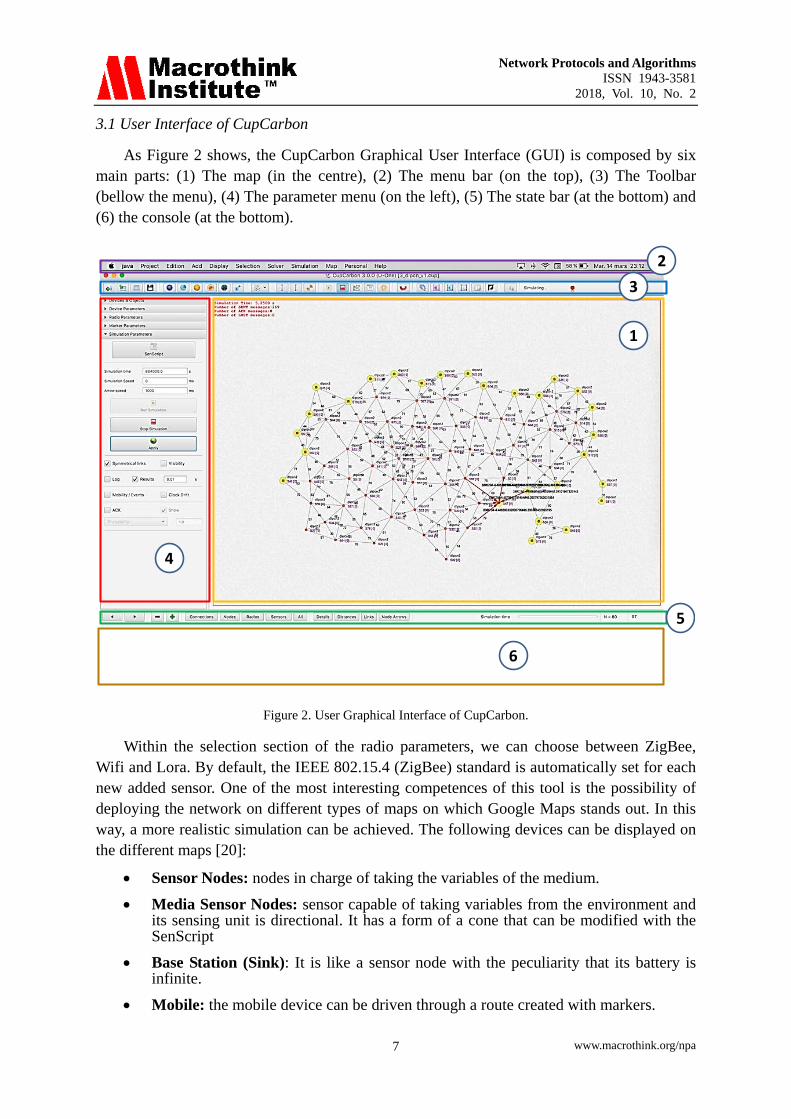
As Figure 2 shows, the CupCarbon Graphical User Interface (GUI) is composed by six main parts: (1) The map (in the centre), (2) The menu bar (on the top), (3) The Toolbar (bellow the menu), (4) The parameter menu (on the left), (5) The state bar (at the bottom) and (6) the console (at the bottom).

2

1

3

4

5

6

Figure 2. User Graphical Interface of CupCarbon.

Within the selection section of the radio parameters, we can choose between ZigBee, Wifi and Lora. By default, the IEEE 802.15.4 (ZigBee) standard is automatically set for each new added sensor. One of the most interesting competences of this tool is the possibility of deploying the network on different types of maps on which Google Maps stands out. In this way, a more realistic simulation can be achieved. The following devices can be displayed on the different maps [20]:

• Sensor Nodes: nodes in charge of taking the variables of the medium. • Media Sensor Nodes: sensor capable of taking variables from the environment and

its sensing unit is directional. It has a form of a cone that can be modified with the SenScript

• Base Station (Sink): It is like a sensor node with the peculiarity that its battery is infinite.

• Mobile: the mobile device can be driven through a route created with markers.


2018, Vol. 10, No. 2


• Markers: these markers can be used for different tasks such as: o Adding sensors can be done randomly delimiting the area on which you want

to deploy. o Creating routes. o Adding or drawing buildings.

Moreover, by extending the Solver section of the menu, we can use different algorithms such as the Jarvis algorithm that, given a cloud of points, surrounds them with lines in the positive direction.

3.2 Example performed in CupCarbon

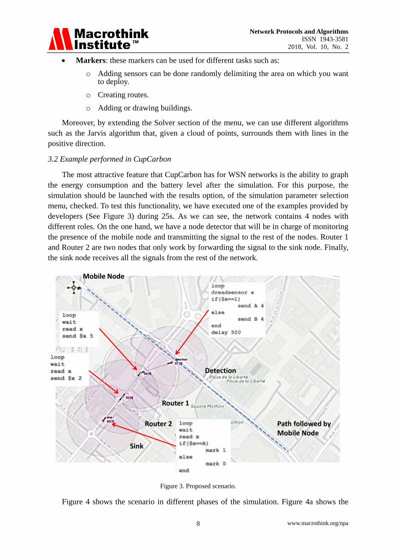
The most attractive feature that CupCarbon has for WSN networks is the ability to graph the energy consumption and the battery level after the simulation. For this purpose, the simulation should be launched with the results option, of the simulation parameter selection menu, checked. To test this functionality, we have executed one of the examples provided by developers (See Figure 3) during 25s. As we can see, the network contains 4 nodes with different roles. On the one hand, we have a node detector that will be in charge of monitoring the presence of the mobile node and transmitting the signal to the rest of the nodes. Router 1 and Router 2 are two nodes that only work by forwarding the signal to the sink node. Finally, the sink node receives all the signals from the rest of the network.

Mobile Node

Detection

Router 1

Router 2

Sink

Path followed byMobile Node

Figure 3. Proposed scenario.

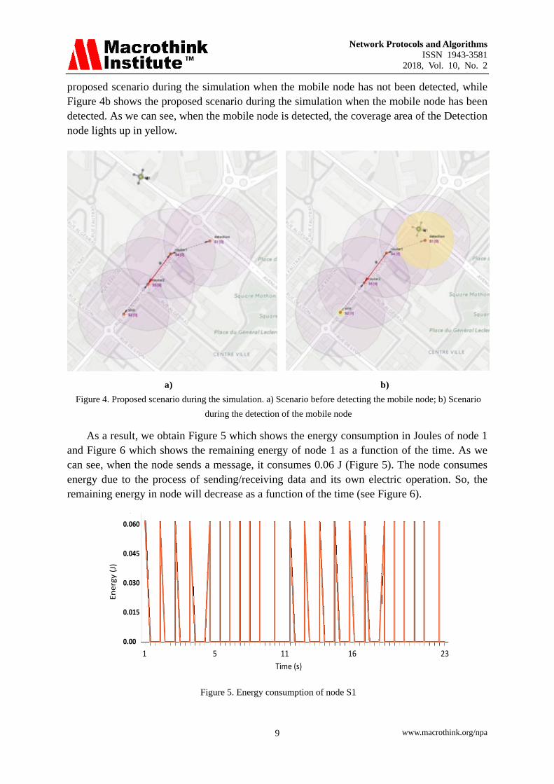
Figure 4 shows the scenario in different phases of the simulation. Figure 4a shows the


2018, Vol. 10, No. 2


proposed scenario during the simulation when the mobile node has not been detected, while Figure 4b shows the proposed scenario during the simulation when the mobile node has been detected. As we can see, when the mobile node is detected, the coverage area of the Detection node lights up in yellow.

a) b) Figure 4. Proposed scenario during the simulation. a) Scenario before detecting the mobile node; b) Scenario

during the detection of the mobile node

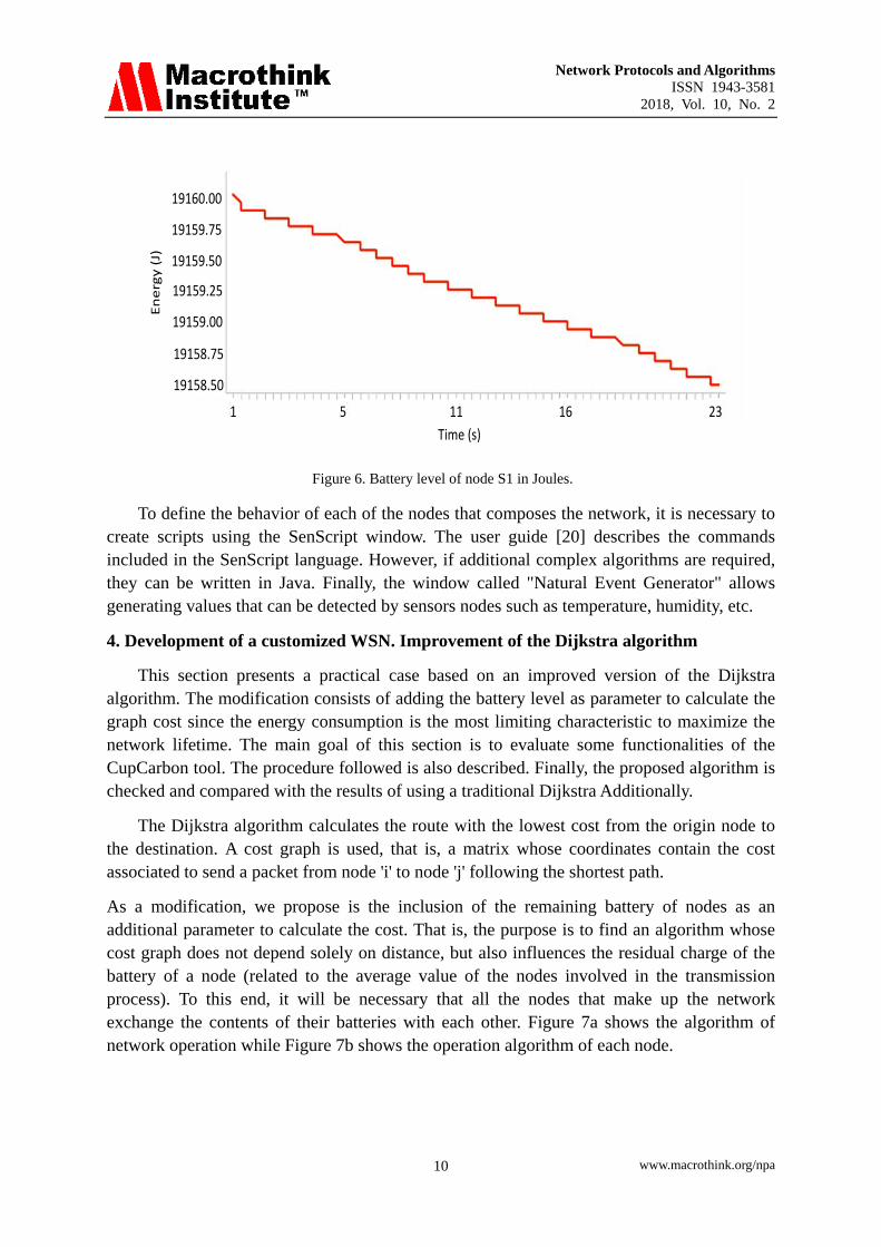
As a result, we obtain Figure 5 which shows the energy consumption in Joules of node 1 and Figure 6 which shows the remaining energy of node 1 as a function of the time. As we can see, when the node sends a message, it consumes 0.06 J (Figure 5). The node consumes energy due to the process of sending/receiving data and its own electric operation. So, the remaining energy in node will decrease as a function of the time (see Figure 6).

Time (s)

Ener

gy(J

)

1 5 11 16 23

0.060

0.045

0.030

0.015

0.00

Figure 5. Energy consumption of node S1


2018, Vol. 10, No. 2


Time (s)

Ener

gy(J

)

1 5 11 16 23

19160.00

19159.75

19159.50

19159.25

19159.00

19158.75

19158.50

Figure 6. Battery level of node S1 in Joules.

To define the behavior of each of the nodes that composes the network, it is necessary to create scripts using the SenScript window. The user guide [20] describes the commands included in the SenScript language. However, if additional complex algorithms are required, they can be written in Java. Finally, the window called "Natural Event Generator" allows generating values that can be detected by sensors nodes such as temperature, humidity, etc.

4. Development of a customized WSN. Improvement of the Dijkstra algorithm

This section presents a practical case based on an improved version of the Dijkstra algorithm. The modification consists of adding the battery level as parameter to calculate the graph cost since the energy consumption is the most limiting characteristic to maximize the network lifetime. The main goal of this section is to evaluate some functionalities of the CupCarbon tool. The procedure followed is also described. Finally, the proposed algorithm is checked and compared with the results of using a traditional Dijkstra Additionally.

The Dijkstra algorithm calculates the route with the lowest cost from the origin node to the destination. A cost graph is used, that is, a matrix whose coordinates contain the cost associated to send a packet from node 'i' to node 'j' following the shortest path.

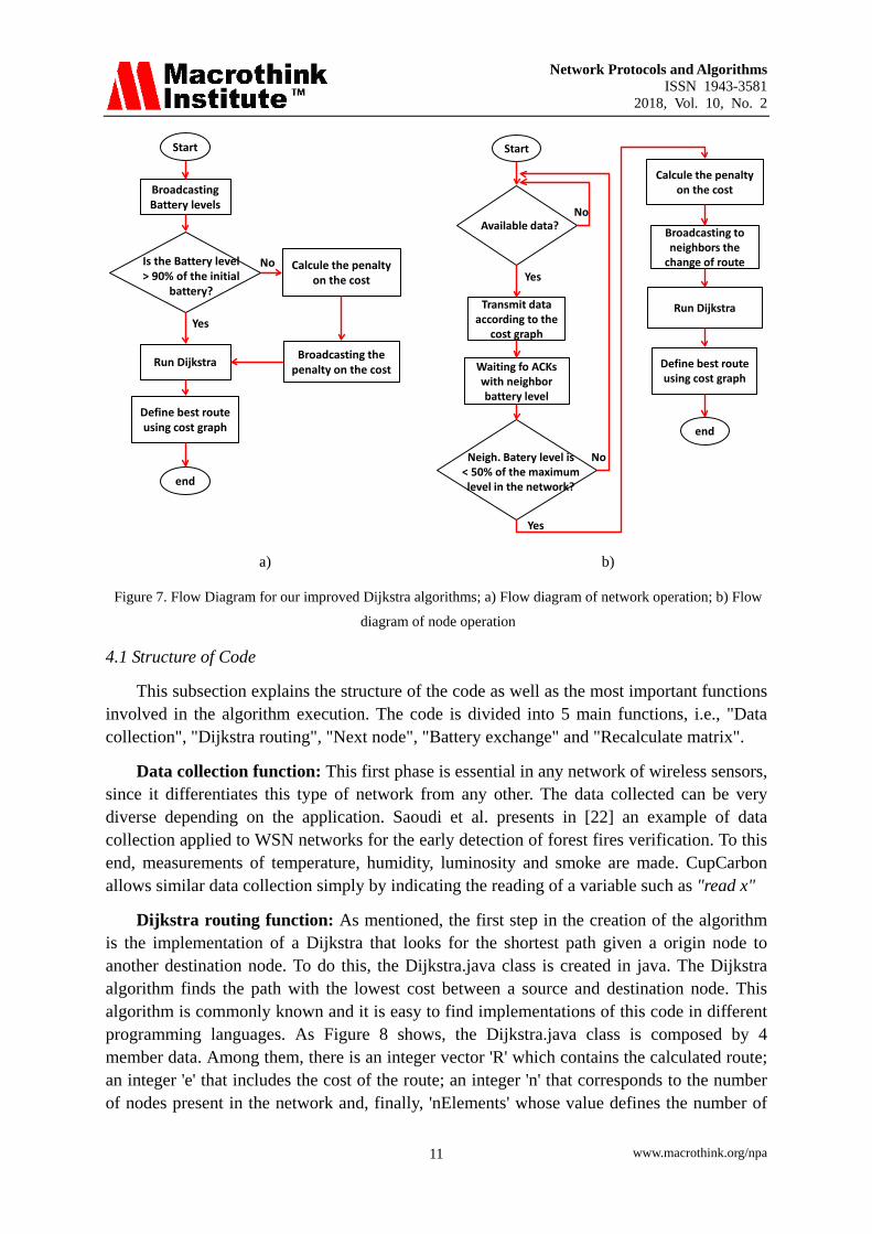
As a modification, we propose is the inclusion of the remaining battery of nodes as an additional parameter to calculate the cost. That is, the purpose is to find an algorithm whose cost graph does not depend solely on distance, but also influences the residual charge of the battery of a node (related to the average value of the nodes involved in the transmission process). To this end, it will be necessary that all the nodes that make up the network exchange the contents of their batteries with each other. Figure 7a shows the algorithm of network operation while Figure 7b shows the operation algorithm of each node.


2018, Vol. 10, No. 2


Start

BroadcastingBattery levels

Is the Battery level> 90% of the initial

battery?

Run Dijkstra

Define best routeusing cost graph

Calcule the penaltyon the cost

Broadcasting thepenalty on the cost

end

Yes

No

Start

Broadcasting to neighbors the

change of route

Available data?

Transmit data according to the

cost graph

Define best routeusing cost graph

Calcule the penaltyon the cost

Run Dijkstra

end

Yes

No

Waiting fo ACKswith neighborbattery level

Neigh. Batery level is< 50% of the maximumlevel in the network?

No

Yes

a) b)

Figure 7. Flow Diagram for our improved Dijkstra algorithms; a) Flow diagram of network operation; b) Flow

diagram of node operation

4.1 Structure of Code

This subsection explains the structure of the code as well as the most important functions involved in the algorithm execution. The code is divided into 5 main functions, i.e., "Data collection", "Dijkstra routing", "Next node", "Battery exchange" and "Recalculate matrix".

Data collection function: This first phase is essential in any network of wireless sensors, since it differentiates this type of network from any other. The data collected can be very diverse depending on the application. Saoudi et al. presents in [22] an example of data collection applied to WSN networks for the early detection of forest fires verification. To this end, measurements of temperature, humidity, luminosity and smoke are made. CupCarbon allows similar data collection simply by indicating the reading of a variable such as "read x"

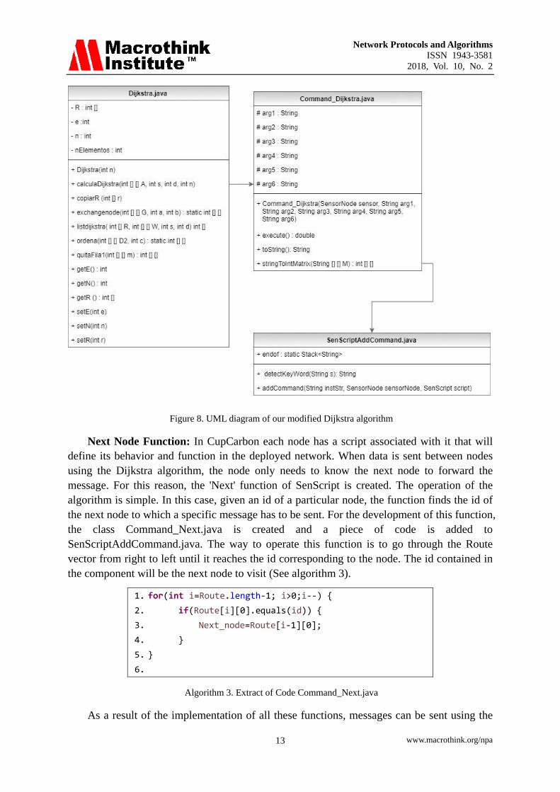
Dijkstra routing function: As mentioned, the first step in the creation of the algorithm is the implementation of a Dijkstra that looks for the shortest path given a origin node to another destination node. To do this, the Dijkstra.java class is created in java. The Dijkstra algorithm finds the path with the lowest cost between a source and destination node. This algorithm is commonly known and it is easy to find implementations of this code in different programming languages. As Figure 8 shows, the Dijkstra.java class is composed by 4 member data. Among them, there is an integer vector 'R' which contains the calculated route; an integer 'e' that includes the cost of the route; an integer 'n' that corresponds to the number of nodes present in the network and, finally, 'nElements' whose value defines the number of


2018, Vol. 10, No. 2


components that the Route vector contains. That is, in a scenario with 5 nodes, if the vector is full, then 'nElements' will be equal to 5. The final method for calculating the route and cost is 'calculateDijkstra (...)'. This method calculates the route and cost for an array whose components contain the cost between two nodes (also called cost graph), source node, destination node and number of nodes in the given network. The mentioned variables are passed by value to the method.

To be able to interpret the Java codes in CupCarbon, it is necessary to create a function in SenScript, so that the Dijkstra algorithm can be used in the scripts of CupCarbon. It is necessary to modify the source code of CupCarbon that can be downloaded for free in [20]. Therefore, the java classes Command_Dijkstra.java and SenScriptAddCommand.java are necessary for implementing this function. The following code fragment is added inside the 'addComand (...)' method (See Algorithm 1).

1. if (inst[0].toLowerCase().equals("dijkstra")) { 2. command = new Command_Dijkstra(sensorNode, inst[1], inst[2], inst[3],

inst[4], inst[5], inst[6]); 3. }

Algorithm 1. Code for Flow SenScriptAddCommand.java.

Each variable 'inst []' is given by a value to the constructor 'Command_Dijkstra (...)' and it corresponds to an argument of the Dijkstra function for SenScript. In the Command_Dijkstra.java class, the value of each of these arguments is defined as presented as Algorithm 2 shows.

1. String tabDist = arg3; 2. String vecRute = arg2; 3. String num = sensor.getScript().getVariableValue(arg4); 4. String source = sensor.getScript().getVariableValue(arg5); 5. String dest = sensor.getScript().getVariableValue(arg6); 6. int n = Double.valueOf(num).intValue(); 7. int s=Double.valueOf(source).intValue(); 8. int d = Double.valueOf(dest).intValue(); 9. String[][] tab = sensor.getScript().getTable(tabDist); 10. String[][] Rute = sensor.getScript().getTable(vecRute); 11. int[][] m = new int[tab.length][tab[0].length]; 12. m=stringToIntMatrix(tab); 13. […] //Code not copied 14. sensor.getScript().addVariable(arg1, coste);

Algorithm 2. Extract of Code Command_Dijkstra.java.

The six arguments defined (arg1, ..., arg6) are specified in the constructor. Each of them corresponds to the cost, the route vector, the cost matrix, the number of nodes in the network, the origin node and, finally, the destination node, respectively. The first two are output arguments and the rest are input arguments.


2018, Vol. 10, No. 2


Figure 8. UML diagram of our modified Dijkstra algorithm

Next Node Function: In CupCarbon each node has a script associated with it that will define its behavior and function in the deployed network. When data is sent between nodes using the Dijkstra algorithm, the node only needs to know the next node to forward the message. For this reason, the 'Next' function of SenScript is created. The operation of the algorithm is simple. In this case, given an id of a particular node, the function finds the id of the next node to which a specific message has to be sent. For the development of this function, the class Command_Next.java is created and a piece of code is added to SenScriptAddCommand.java. The way to operate this function is to go through the Route vector from right to left until it reaches the id corresponding to the node. The id contained in the component will be the next node to visit (See algorithm 3).

1. for(int i=Route.length-1; i>0;i--) { 2. if(Route[i][0].equals(id)) { 3. Next_node=Route[i-1][0]; 4. } 5. } 6.

Algorithm 3. Extract of Code Command_Next.java

As a result of the implementation of all these functions, messages can be sent using the


2018, Vol. 10, No. 2


Dijkstra algorithm in a CupCarbon script that will be assigned to each node of the network. Algorithm 4 shows the necessary code to be defined in a node for the sending a 'hello' message from a origin node 's' to a destination node 'd'.

1. dijkstra c r A $n $s $d 2. atget id f 3. next t r $f 4. send hola $t

Algorithm 4. Fragment of ‘script.csc’ that makes use of Dijkstra algorithm.

First, the function 'dijkstra' is called, calculating the route 'r' with an associated cost 'c'. Then the next node to which the message is to be sent is calculated given the id of the current node 'f' and, finally the message 'hello' is sent to the next node 't'.

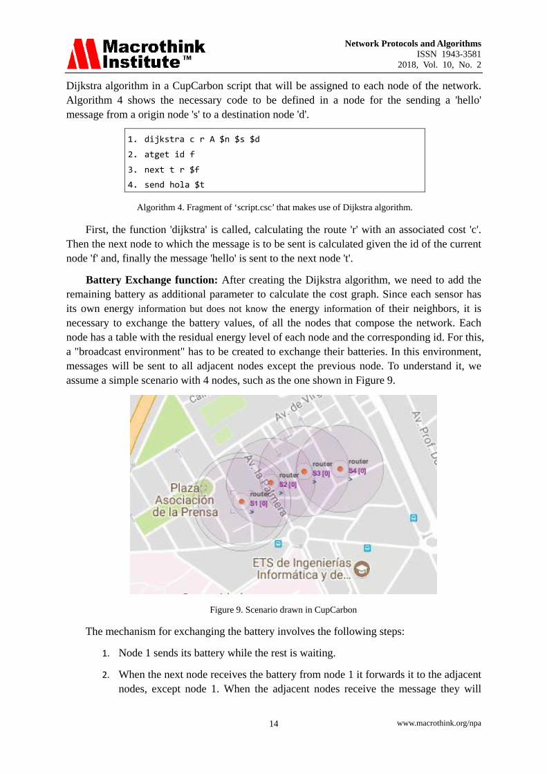
Battery Exchange function: After creating the Dijkstra algorithm, we need to add the remaining battery as additional parameter to calculate the cost graph. Since each sensor has its own energy information but does not know the energy information of their neighbors, it is necessary to exchange the battery values, of all the nodes that compose the network. Each node has a table with the residual energy level of each node and the corresponding id. For this, a "broadcast environment" has to be created to exchange their batteries. In this environment, messages will be sent to all adjacent nodes except the previous node. To understand it, we assume a simple scenario with 4 nodes, such as the one shown in Figure 9.

Figure 9. Scenario drawn in CupCarbon

The mechanism for exchanging the battery involves the following steps:

1. Node 1 sends its battery while the rest is waiting.

2. When the next node receives the battery from node 1 it forwards it to the adjacent nodes, except node 1. When the adjacent nodes receive the message they will


2018, Vol. 10, No. 2


forward it to their neighboring nodes and so on until all the sensors know the battery of 1.

3. The next node, node 2, sends the battery it has repeating steps 1 and 2.

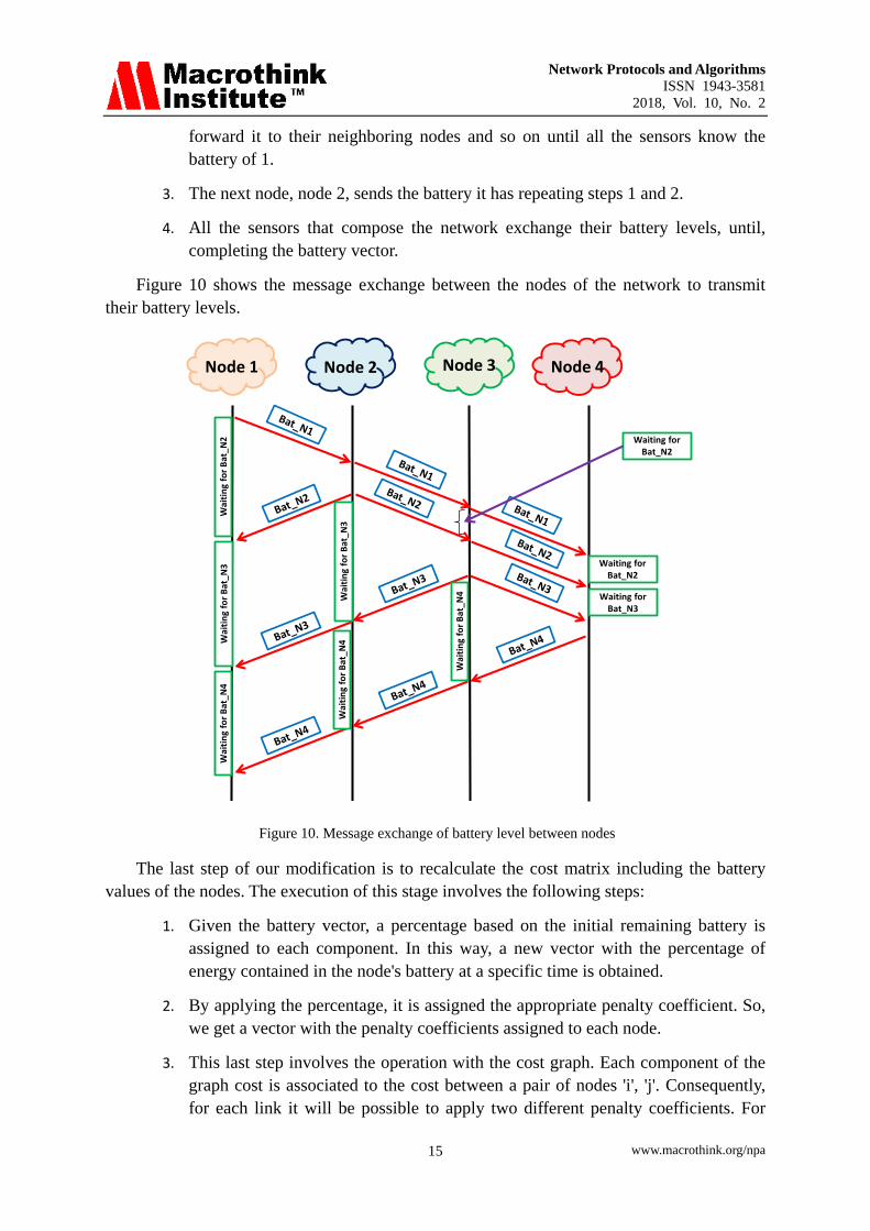
4. All the sensors that compose the network exchange their battery levels, until, completing the battery vector.

Figure 10 shows the message exchange between the nodes of the network to transmit their battery levels.

Node 1 Node 2 Node 3 Node 4

Wai

ting

forB

at_N

2W

aitin

gfo

rBat

_N4

Wai

ting

forB

at_N

3

Wai

ting

forB

at_N

3W

aitin

gfo

rBat

_N4

Wai

ting

forB

at_N

4

Waiting forBat_N2

Waiting forBat_N3

Waiting forBat_N2

Figure 10. Message exchange of battery level between nodes

The last step of our modification is to recalculate the cost matrix including the battery values of the nodes. The execution of this stage involves the following steps:

1. Given the battery vector, a percentage based on the initial remaining battery is assigned to each component. In this way, a new vector with the percentage of energy contained in the node's battery at a specific time is obtained.

2. By applying the percentage, it is assigned the appropriate penalty coefficient. So, we get a vector with the penalty coefficients assigned to each node.

3. This last step involves the operation with the cost graph. Each component of the graph cost is associated to the cost between a pair of nodes 'i', 'j'. Consequently, for each link it will be possible to apply two different penalty coefficients. For


2018, Vol. 10, No. 2


this reason, the worst case is assumed, that is, the highest coefficient. Algorithm 5 shows the necessary code to perform this step. If the component is equal to ∞, that is 999, implies the route in unreachable through this node.

1. for(int i=0; i<coef.length; i++) {

2. for(int j=0; j<coef.length; j++) {

3. if(m[i][j]!=999){

4. if(coef[i]>coef[j]) {

6. m[i][j]=(int) (m[i][j]*coef[i]);

7. }else {

8. m[i][j]=(int) (m[i][j]*coef[j]);

9. }

10. }

11. } 12. }

Algorithm 5. Fragment code for calculating the matrix costs.

4.2 Simulations Results

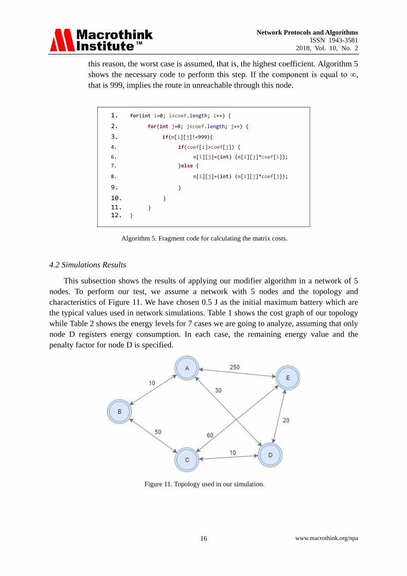
This subsection shows the results of applying our modifier algorithm in a network of 5 nodes. To perform our test, we assume a network with 5 nodes and the topology and characteristics of Figure 11. We have chosen 0.5 J as the initial maximum battery which are the typical values used in network simulations. Table 1 shows the cost graph of our topology while Table 2 shows the energy levels for 7 cases we are going to analyze, assuming that only node D registers energy consumption. In each case, the remaining energy value and the penalty factor for node D is specified.

Figure 11. Topology used in our simulation.


2018, Vol. 10, No. 2


Table 1. Matrix of distances for topology of Figure 11.

Matrix of Distance Nodes

A (i=0) B (i=1) C (i=2) D (i=3) E (i=4)

A (i=0) ∞ 10 ∞ 30 100

B (i=1) 10 ∞ 50 ∞ ∞

C (i=2) ∞ 50 ∞ 10 60

D (i=3) 30 ∞ 10 ∞ 20

E (i=4) 250 ∞ 60 20 ∞

Table 2. Battery vector of topology of Figure 11.

Parameters Cases

1 2 3 4 5 6 7

Battery percentaje 100% 90% 70% 50% 30% 10% 0%

Coeficients 1 1 1,5 2,1 4,1 5,1 999*

Energy

Vector (J)

i=0 500 500 500 500 500 500 500

i=1 500 500 500 500 500 500 500

i=2 500 500 500 500 500 500 500

i=3 500 450 350 250 150 50 0

i=4 500 500 500 500 500 500 500

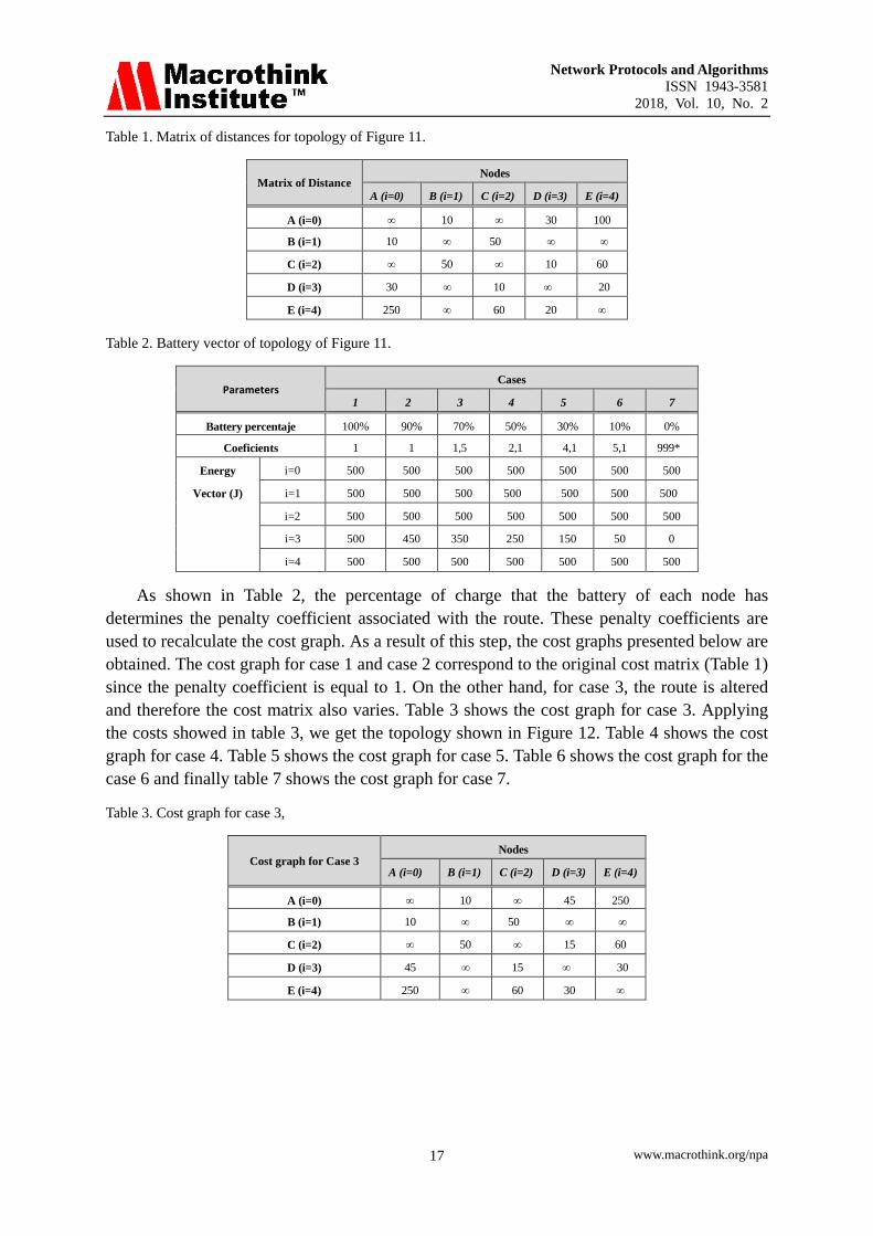
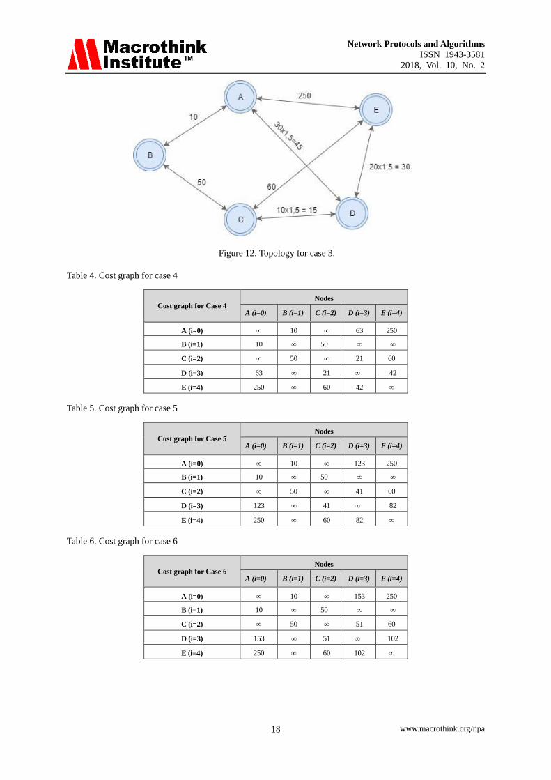
As shown in Table 2, the percentage of charge that the battery of each node has determines the penalty coefficient associated with the route. These penalty coefficients are used to recalculate the cost graph. As a result of this step, the cost graphs presented below are obtained. The cost graph for case 1 and case 2 correspond to the original cost matrix (Table 1) since the penalty coefficient is equal to 1. On the other hand, for case 3, the route is altered and therefore the cost matrix also varies. Table 3 shows the cost graph for case 3. Applying the costs showed in table 3, we get the topology shown in Figure 12. Table 4 shows the cost graph for case 4. Table 5 shows the cost graph for case 5. Table 6 shows the cost graph for the case 6 and finally table 7 shows the cost graph for case 7.

Table 3. Cost graph for case 3,

Cost graph for Case 3 Nodes

A (i=0) B (i=1) C (i=2) D (i=3) E (i=4)

A (i=0) ∞ 10 ∞ 45 250

B (i=1) 10 ∞ 50 ∞ ∞

C (i=2) ∞ 50 ∞ 15 60

D (i=3) 45 ∞ 15 ∞ 30

E (i=4) 250 ∞ 60 30 ∞


2018, Vol. 10, No. 2


Figure 12. Topology for case 3.

Table 4. Cost graph for case 4


A (i=0) B (i=1) C (i=2) D (i=3) E (i=4)

A (i=0) ∞ 10 ∞ 63 250

B (i=1) 10 ∞ 50 ∞ ∞

C (i=2) ∞ 50 ∞ 21 60

D (i=3) 63 ∞ 21 ∞ 42

E (i=4) 250 ∞ 60 42 ∞



A (i=0) B (i=1) C (i=2) D (i=3) E (i=4)

A (i=0) ∞ 10 ∞ 123 250

B (i=1) 10 ∞ 50 ∞ ∞

C (i=2) ∞ 50 ∞ 41 60

D (i=3) 123 ∞ 41 ∞ 82

E (i=4) 250 ∞ 60 82 ∞



A (i=0) B (i=1) C (i=2) D (i=3) E (i=4)

A (i=0) ∞ 10 ∞ 153 250

B (i=1) 10 ∞ 50 ∞ ∞

C (i=2) ∞ 50 ∞ 51 60

D (i=3) 153 ∞ 51 ∞ 102

E (i=4) 250 ∞ 60 102 ∞


2018, Vol. 10, No. 2




A (i=0) B (i=1) C (i=2) D (i=3) E (i=4)

A (i=0) ∞ 10 ∞ 45 250

B (i=1) 10 ∞ 50 ∞ ∞

C (i=2) ∞ 50 ∞ ∞ 60

D (i=3) ∞ ∞ ∞ ∞ ∞

E (i=4) 250 ∞ 60 ∞ ∞

Finally, assuming the cases shown in Table 2 different routes are established to check how the algorithm would vary in the choice of the best path. Table 8 shows the result of applying our proposed algorithm when different routes are selected.

Table 8. Results of routes

Routes Cases

1 2 3 4 5 6 7

C -> E C->D->E C->D->E C->D->E C->E C->E C->E C->E

Cost 30 30 45 60 60 60 60

A -> C A->D->C A->D->C A->B->C A->B->C A->B->C A->B->C A->B->C

Cost 40 40 60 60 60 60 60

A-> E A->D->E A->D->E A->D->E A->D->E A->D->E A->E A->E

Cost 50 50 75 105 205 250 250

In the last test, we analyzed how the battery levels would vary in a continuous sending in the topology of Figure 13 where the algorithm shown in Figure 7 is applied. In this case, all nodes register energy consumption being node D the one that consumes more energy. This algorithm allows us to dynamically change the route depending on the battery levels of each node, compared to the maximum battery value of the adjacent neighbors.

Best route accordingto Dijkstra

Alternative route whenour algoritm is used

Figure 13. Topology used in our test


2018, Vol. 10, No. 2


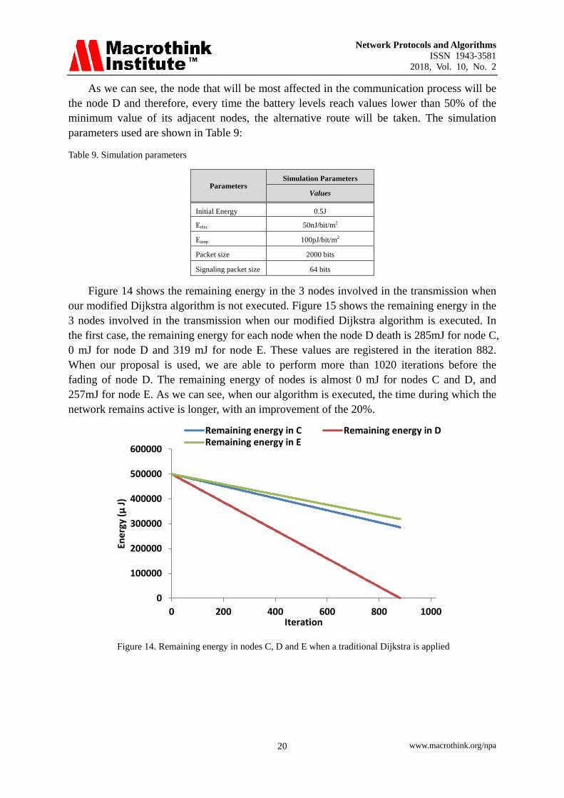
As we can see, the node that will be most affected in the communication process will be the node D and therefore, every time the battery levels reach values lower than 50% of the minimum value of its adjacent nodes, the alternative route will be taken. The simulation parameters used are shown in Table 9:

Table 9. Simulation parameters

Parameters Simulation Parameters

Values

Initial Energy 0.5J

Eelec 50nJ/bit/m2

Eamp 100pJ/bit/m2

Packet size 2000 bits

Signaling packet size 64 bits

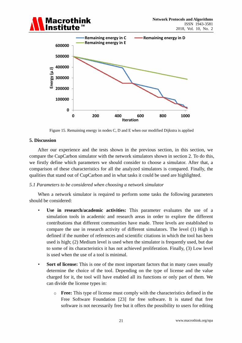
Figure 14 shows the remaining energy in the 3 nodes involved in the transmission when our modified Dijkstra algorithm is not executed. Figure 15 shows the remaining energy in the 3 nodes involved in the transmission when our modified Dijkstra algorithm is executed. In the first case, the remaining energy for each node when the node D death is 285mJ for node C, 0 mJ for node D and 319 mJ for node E. These values are registered in the iteration 882. When our proposal is used, we are able to perform more than 1020 iterations before the fading of node D. The remaining energy of nodes is almost 0 mJ for nodes C and D, and 257mJ for node E. As we can see, when our algorithm is executed, the time during which the network remains active is longer, with an improvement of the 20%.

0

100000

200000

300000

400000

500000

600000

0 200 400 600 800 1000

Ener

gy (μ

J)

Iteration

Remaining energy in C Remaining energy in DRemaining energy in E

Figure 14. Remaining energy in nodes C, D and E when a traditional Dijkstra is applied


2018, Vol. 10, No. 2


0

100000

200000

300000

400000

500000

600000

0 200 400 600 800 1000

Ener

gy (μ

J)

Iteration

Remaining energy in C Remaining energy in DRemaining energy in E

Figure 15. Remaining energy in nodes C, D and E when our modified Dijkstra is applied

5. Discussion

After our experience and the tests shown in the previous section, in this section, we compare the CupCarbon simulator with the network simulators shown in section 2. To do this, we firstly define which parameters we should consider to choose a simulator. After that, a comparison of these characteristics for all the analyzed simulators is compared. Finally, the qualities that stand out of CupCarbon and in what tasks it could be used are highlighted.

5.1 Parameters to be considered when choosing a network simulator

When a network simulator is required to perform some tasks the following parameters should be considered:

• Use in research/academic activities: This parameter evaluates the use of a simulation tools in academic and research areas in order to explore the different contributions that different communities have made. Three levels are established to compare the use in research activity of different simulators. The level (1) High is defined if the number of references and scientific citations in which the tool has been used is high; (2) Medium level is used when the simulator is frequently used, but due to some of its characteristics it has not achieved proliferation. Finally, (3) Low level is used when the use of a tool is minimal.

• Sort of license: This is one of the most important factors that in many cases usually determine the choice of the tool. Depending on the type of license and the value charged for it, the tool will have enabled all its functions or only part of them. We can divide the license types in:

o Free: This type of license must comply with the characteristics defined in the Free Software Foundation [23] for free software. It is stated that free software is not necessarily free but it offers the possibility to users for editing


2018, Vol. 10, No. 2


it, coping it, executing it, distributing it and improving it. In this way, we have four freedoms: (1) run the program for any purpose, (2) study how the program works and adapt it to the needs we have, (3) distribute the code from one user to another, and (4) distribute the modified code to others.

o Commercial: Licenses that have certain restrictions for the user and users have to pay for disabling these restrictions.

• Curve of learning: With this parameter, it is defined the level of demand of the tool to achieve an adequate management. For its measurement, previous knowledge about protocols and standards used for communicating networks and programming as well as the didactic use of the tool are taken into account. In this last sense, there are simulators that, in terms of interaction, are extremely user-friendly since they allow configuring network elements in an intuitive way. The evaluation of this parameter is divided into: (1) High level, when high prior knowledge in networks and programming are required; (2) Medium when the entire learning load is focused on the configuration of network devices through console commands; and (3) Low when the dynamic use tools in which the interaction with the user is very intuitive.

• Platforms: This parameter specifies the operating systems for which the program can be executed without any problem.

• Graphical Interface: With this parameter we define the friendliness of the tool to the user. The ranges are:

o High. It is possible to perform all the tasks through the graphical interface so the level of programming required is minimal.

o Medium. The graphical interface facilitates its use, but some implementations must be done through programming.

o Low. The tool does not have a graphical interface or, if it has one, it is not friendly to the user, so the programming of each element is necessary.

• Results through graphs: For a network simulator, the final end is to evaluate the network in a real environment so it is necessary to take measurements of some variables. One way to interpret the data obtained is to graph them. Depending on how powerful and/or friendly the tool is for this purpose, the following categories can be defined:

o Good. The tool has its own modules for generating graphics and statistics that can be manipulated from the same simulator or exported to a specialized processor.

o Acceptable. These simulators can generate statistical data, but they need an external tool to process them and present them in a friendly manner to the user.

o Limited. In this case, the tools do not have their own module for generating


2018, Vol. 10, No. 2


graphics. The statistical information can be represented in text files that need an external extension for its presentation.

• Supported technologies and layer 2-3 protocols: This parameter refers to the lists the technologies and layer 2-3 protocols of the OSI Model each simulator supports. The simulator that does not support all protocols should implement them by generating code or adapting pre-existing components.

• Traffic modeled: This parameter is important since it determines the types of applications, protocols and services that each simulator is able to simulate. In this way, we will classify the simulators based on the amount of services they support, following the criteria:

o High. Simulators that allow generating a great variety of application traffic.

o Medium. Simulators with the ability to generate traffic from the most common applications.

o Low. In this case, it is not possible to configure traffic distributions that allow an in deep academic analysis, or failing that they do not have modules or extensions for this end.

• Programming Language: It defines the programming languages needed to develop our networks in each simulation.

• Energy modeling: Energy modeling is a critical analysis for WSN networks because the nodes are usually powered by batteries. Energy efficiency is perhaps one of the parameters that have become more important for this type of networks during the planning of sensor networks with the aim of prolonging their life time. Through this parameter, it is evaluated if the different simulators have tools for energy modeling.

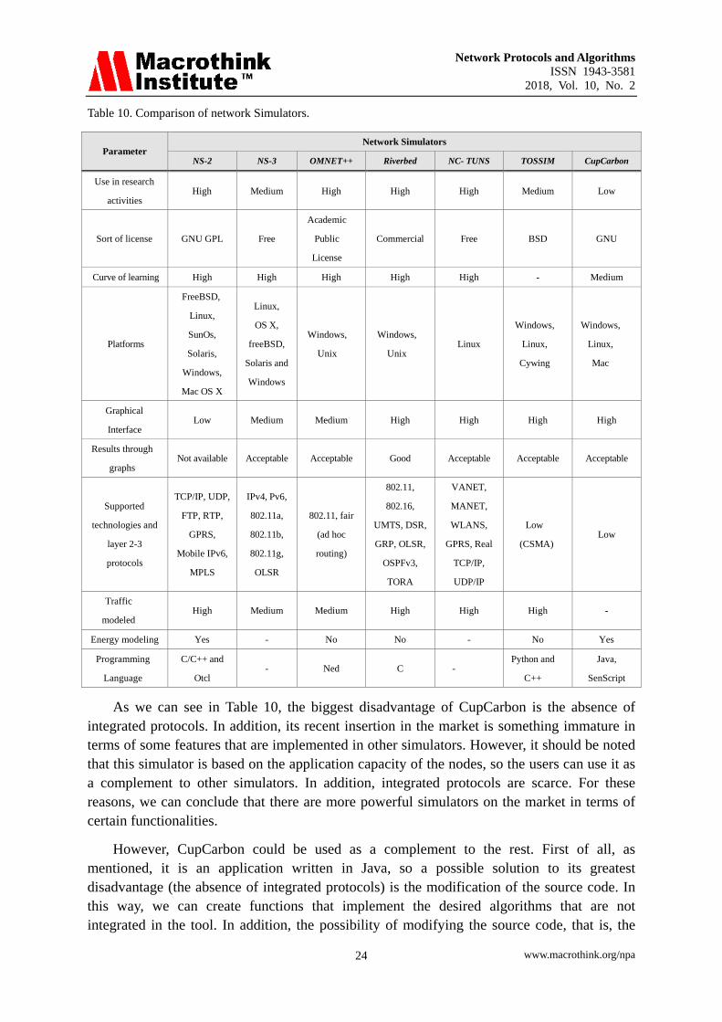
5.2 Comparison

Finally, the Table 10 shows the comparison of CupCarbon and the simulators presented in Section 3.


2018, Vol. 10, No. 2


Table 10. Comparison of network Simulators.

Parameter Network Simulators

NS-2 NS-3 OMNET++ Riverbed NC- TUNS TOSSIM CupCarbon

Use in research

activities High Medium High High High Medium Low

Sort of license GNU GPL Free

Academic

Public

License

Commercial Free BSD GNU

Curve of learning High High High High High - Medium

Platforms

FreeBSD,

Linux,

SunOs,

Solaris,

Windows,

Mac OS X

Linux,

OS X,

freeBSD,

Solaris and

Windows

Windows,

Unix

Windows,

Unix Linux

Windows,

Linux,

Cywing

Windows,

Linux,

Mac

Graphical

Interface Low Medium Medium High High High High

Results through

graphs Not available Acceptable Acceptable Good Acceptable Acceptable Acceptable

Supported

technologies and

layer 2-3

protocols

TCP/IP, UDP,

FTP, RTP,

GPRS,

Mobile IPv6,

MPLS

IPv4, Pv6,

802.11a,

802.11b,

802.11g,

OLSR

802.11, fair

(ad hoc

routing)

802.11,

802.16,

UMTS, DSR,

GRP, OLSR,

OSPFv3,

TORA

VANET,

MANET,

WLANS,

GPRS, Real

TCP/IP,

UDP/IP

Low

(CSMA) Low

Traffic

modeled High Medium Medium High High High -

Energy modeling Yes - No No - No Yes

Programming

Language

C/C++ and

Otcl - Ned C -

Python and

C++

Java,

SenScript

As we can see in Table 10, the biggest disadvantage of CupCarbon is the absence of integrated protocols. In addition, its recent insertion in the market is something immature in terms of some features that are implemented in other simulators. However, it should be noted that this simulator is based on the application capacity of the nodes, so the users can use it as a complement to other simulators. In addition, integrated protocols are scarce. For these reasons, we can conclude that there are more powerful simulators on the market in terms of certain functionalities.

However, CupCarbon could be used as a complement to the rest. First of all, as mentioned, it is an application written in Java, so a possible solution to its greatest disadvantage (the absence of integrated protocols) is the modification of the source code. In this way, we can create functions that implement the desired algorithms that are not integrated in the tool. In addition, the possibility of modifying the source code, that is, the


2018, Vol. 10, No. 2


open source is another great advantage. On the other hand, CupCarbon has the possibility of observing the consumption of resources that occur due to the nature of urban networks. The sensors can be displayed directly on the map. Additionally, the graphical interface is another of its advantages; it is intuitive for the user and allows performing all the functionalities through it. Another advantage is the lack of important prerequisite requirements. The only ones we need is to access to the program and programming in Java. For these reasons, intuitive interface and reduced prior knowledge, it is a suitable tool for academic or networking environments. Finally, the presence of energy modeling that can be plotted is another advantage since it is an important parameter to be tested in WSNs.

6. Conclusion and Future work

WSN is a technology in full development and with great future. Currently, there are several applications that make use of them. For this reason, there are numerous network simulators in the market to emulate the operation of this type of networks that provide different functionalities. Consequently, the most appropriate simulator will depend on the application we wish to develop.

In this paper, the CupCarbon network simulator has been analyzed. To evaluate the ease of use and the results it offers, a modified Dijkstra algorithm has been designed. This modification includes the battery level of the nodes as an additional parameter to be considered in order to calculate the best route. As a result of our modified Dijkstra, it is possible to keep all the nodes of the network alive for 20% more time than using a conventional Dijkstra algorithm. Additionally, it is verified that the total energy dissipated from the network is distributed more equitably. Consequently, a more efficient network is achieved.

Finally, the following conclusions can be drawn. The evaluation of CupCarbon has not been satisfactory enough, although, given its continuous updates, its perfection and full development of some of its most interesting features are expected, such as the possibility of migration of code to the Arduino platform. Although CupCarbon has allowed us to develop the algorithms that we wanted, the fact of having to work with different programming languages makes it not recommended for certain applications. However, CupCarbon could be used as a teaching complement in subjects related to networks.

As future work, we want to see the possibility of developing other protocols focused on saving energy consumption for WSNs. Finally, we want to check other scenarios and situations where the use of wireless nodes and mobile nodes can help us to solve dangerous events [24].

References

[1] Kumbhar, A., Koohifar, F., Güvenç, I. and, Mueller, B., “A survey on legacy and emerging technologies for public safety communications”. IEEE Communications Surveys & Tutorials. Vol. 19,


2018, Vol. 10, No. 2


Issue 1. Pp.97-124. 2017. DOI: 10.1109/COMST.2016.2612223 [2] Garcia, M., Bri, D., Sendra, R. and, Lloret, J., “Practical deployments of wireless sensor networks: a survey”, International Journal on Advances in Networks and Services. Vol. 3. Issue 1 & 2. Pp. 170-185. 2010. DOI: 0.1.1.681.7101 [3] Yetgin, H., Cheung, K. T. K., El-Hajjar, M. and, Hanzo, L. H., “A survey of network lifetime maximization techniques in wireless sensor networks”. IEEE Communications Surveys & Tutorials. Vol. 19. Issue 2. Pp. 828-854, 2017. DOI: 0.1109/COMST.2017.2650979 [4] Lloret, J., Garcia, M., Bri, D. and, Sendra, S., “A wireless sensor network deployment for rural and forest fire detection and verification”. Sensors. Vol. 9. Issue 11. Pp. 8722-8747. 2009. DOI: 10.3390/s91108722 [5] Azizi, R. “Consumption of energy and routing protocols in wireless sensor network”. Network Protocols and Algorithms. Vol. 8, Issue 3. Pp.76-87. 2016. DOI: https://doi.org/10.5296/npa.v8i3.10257 [6] Liang, J., Liu, M., & Kui, X. “A survey of coverage problems in wireless sensor networks”. Sensors & Transducers. Vol. 163. Issue 1, Pp. 240-246. 2014. DOI:10.1.1.433.8178 [7] Fall, K. and Varadhan, K. The ns Manual (formerly ns Notes and Documentation). The VINT project, 47.2015. Available at: https://www.isi.edu/nsnam/ns/doc/ns_doc.pdf [Last Access: June 11, 2018] [8] Rajaram, M. L., Kougianos, E., Mohanty, S. P. and, Choppali, U.,”Wireless sensor network simulation frameworks: A tutorial review: MATLAB/Simulink bests the rest”. IEEE Consumer Electronics Magazine. Vol. 5, Issue 2. Pp. 63-69. 2016. DOI: 10.1109/MCE.2016.2519051 [9] Korkalainen, M., Sallinen, M., Kärkkäinen, N. and, Tukeva, P., “Survey of wireless sensor networks simulation tools for demanding applications”. In proc. of the Fifth International Conference on Networking and Services (ICNS'09). April 20-25, 2009. Valencia, Spain (pp. 102-106). DOI: 10.1109/ICNS.2009.75 [10] Ns-3 Network simulator .Available at: https://www.nsnam.org [Last Access: June 11, 2018] [11] Henderson, T. R., Roy, S., Floyd, S. and, Riley, G.F., “Ns-3 Project Goals”. in proc. of the 2006 workshop on ns-2: the IP network simulator (WNS2 '06). October 10, 2006. Pisa, Italy (pp. 13-20). DOI: 10.1145/1190455.1190468 [12] Omnet++ Network simulator. Available at: https://www.omnetpp.org/ [Last Access: June 11, 2018] [13] Chen, F., Dietrich, I., German, R. and, Dressler, F., “An energy model for simulation studies of wireless sensor networks using omnet++”. PIK-Praxis der Informationsverarbeitung und Kommunikation, 32(2). Pp. 133-138. 2009. DOI: https://doi.org/10.1515/piko.2009.0023 [14] Riverved Network Simulator. Available at: https://www.riverbed.com/ [Last Access: June 11, 2018] [15] Hammoodi, I. S., Stewart, B. G., Kocian, A. and, McMeekin, S. G., "A Comprehensive Performance Study of OPNET Modeler for ZigBee Wireless Sensor Networks,", In proc. of the Third International Conference on Next Generation Mobile Applications, Services and Technologies (NGMAST 2009), September 16 -18, 2009. Cardiff, Wales, (pp. 357-362). DOI: 10.1109/NGMAST.2009.12 [16] Wang S. Y. and Huang Y.M., “NCTUNS Distributed Network Emulator”, Internet Journal. Vol. 4, Issue 2. Pp.66-94. 2012. DOI:10.1.1.666.853 [17] “TOSSIM”, In TinyOS web site. Available at: http://tinyos.stanford.edu/tinyos-wiki/index.php/TOSSIM. [Last Access: June 11, 2018] [18] Perla, E., Catháin, A. Ó., Carbajo, R. S., Huggard, M., & Mc Goldrick, C., “PowerTOSSIM z: realistic energy modelling for wireless sensor network environments”, In proc. of The 11-th ACM International Conference on Modeling, Analysis and Simulation of Wireless and Mobile Systems, October 31 - 31, 2008. Vancouver, British Columbia, Canada. (Pp. 35-42). DOI:10.1145/1454630.1454636

https://www.isi.edu/nsnam/ns/doc/ns_doc.pdf

https://www.nsnam.org/

https://www.omnetpp.org/

https://www.riverbed.com/

http://tinyos.stanford.edu/tinyos-wiki/index.php/TOSSIM


2018, Vol. 10, No. 2


[19] Kellner, A., Behrends, K. and, Hogrefe, D., “Simulation Environments for Wireless Sensor Networks”, Technical Report, IFI-TB-2010-04, Pp. 1-11. June 2010. Available at: https://pdfs.semanticscholar.org/ab88/d8d685c782d67129e2866c628be904d50988.pdf [Last Access: June 11, 2018] [20] CupCarbon User Guide. Available at: http://www.cupcarbon.com/cupcarbon_ug.html [Last Access: June 11, 2018] [21] CupCarbon network simulator. Available at: http://www.cupcarbon.com/ [Last Access: June 11, 2018] [22] Saoudi, M., Bounceur, A., Euler, R. and, Kechadi, T., “Data Mining Techniques Applied to Wireless Sensor Networks for Early Forest Fire Detection”, In Proc. of the International Conference on Internet of things and Cloud Computing. March 22-23, 2016. Cambridge, United Kingdom. (Article No. 71) DOI:10.1145/2896387.2900323 [23] Free Software Foundation. Available at: https://www.fsf.org/?set_language=es. [Last Access: June 11, 2018] [24] Cambra, C., Sendra, S., Lloret, J. and, Parra, L., “Ad hoc network for emergency rescue system based on unmanned aerial vehicles”. Network Protocols and Algorithms. Vol. 7, Issue 4. Pp. 72-89. 2016. DOI: https://doi.org/10.5296/npa.v7i4.8816

Copyright Disclaimer

Copyright reserved by the author(s).

This article is an open-access article distributed under the terms and conditions of the Creative Commons Attribution license (http://creativecommons.org/licenses/by/3.0/).

http://www.cupcarbon.com/cupcarbon_ug.html

http://www.cupcarbon.com/

https://www.fsf.org/?set_language=es

evaluation of cupcarbon network simulator for wireless

Documents