Evaluation of design waves considering climate change

P Satyavathi, E Roshin, Prerna Bansal, Shreyas Bhat, Pooja Jain and M C Deo

Indian Institute of Technology Bombay, 400076 India

Workshop at Liverpool, Sept. 11, 2017

Background

Structures in the sea are designed using the significant wave height with 100 year’s

return. This value may change in future due to climate change.

Aim :

To evaluate significant wave heights (Hs) with 100-year return

along the entire Indian coastline considering climate change

Procedure :

Consider series of 91 locations around the coastline of India.

Consider historical as well as projected (future) wind data.

Generate Hs for past and future ~30 yr time slices.

Fit statistical distributions and derive 100-year Hs.

Compare such design waves based on past and projected wave data.

Understand amount of variations if the input wind is changed. 2

Locations of interest along the 7500 km long Indian coastline All locations: water depth = 10 – 20 m; ~ 75 km away

3

Arabian Sea

Bay of Bengal

Indian Ocean

-Subjected to reversing SW and NE monsoons, -High seasonality effects, -4.8 cyclones/year, - deep and narrow shelf

-Subjected to SW monsoon with strong waves. -Has high swell dominance. -1.8 cyclones/year -Shallow, wide conti. shelf,

3

To generate waves: Numerical Wave Model: Mike-21 SW, of DHI

Governing equation:

4

-Wind data used to generate waves- An ensemble average of 3 regional climate models (RCMs) available under: CMIP5 Coordinated Regional Downscaling Experiment (CORDEX), South Asia Reg-CM4 (LMDZ), RegCM4 (ESM-LR), SMHI-RCA4 (ECearth),

(Note: RCMs differ from each other due to different modelling of underlying physical processes, use of alternative numerical schemes, boundary conditions.

By taking an ensemble mean of available RCM’s uncertainties in individual RCM’s can be minimized.)

- Past time slice: 27 years (1979-2005) Future time slice: 27 years (2006-2032) Future warming scenario: RCP 4.5 (moderate pathway, rise in temp. = 2.4 deg. C; CO2 equivalent = 650 ppm) - Resolution: 0.44 x 0.44 deg. sq.; 1 day

Wind data pre-processing: -Bias removal – by quantile mapping with CFSR wind

0.5 ̊ x 0.5 ̊ grid resolution; 6 hour temporal resolution - Required re-gridding by bilinear interpolation

5

Model domain and bathymetry Digitized NHO charts Area within 19⁰S to 30⁰ N and 20⁰E to 110⁰ E Mesh size: 1.5◦ (From 40◦ S to 0 ◦), 0.75 ◦ (Above 0 ◦ Lat.) and 0.25 ◦ (along coastline)

6

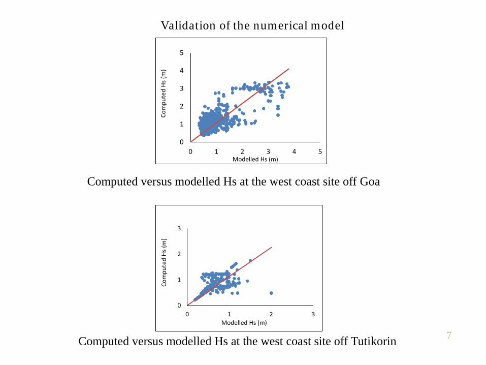
Validation of the numerical model

0

1

2

3

4

5

0 1 2 3 4 5Co

mpu

ted

Hs (m

) Modelled Hs (m)

Computed versus modelled Hs at the west coast site off Goa

0

1

2

3

0 1 2 3

Com

pute

d Hs

(m)

Modelled Hs (m)

Computed versus modelled Hs at the west coast site off Tutikorin 7

Trends of annual average and annual mean Hs were studied.

8

9

Wave rose diagrams for past and future data compared. (Ex.: site:P5)

PDF’s of Hs for past and future compared. (Ex. : Site: P5)

- West coast sites westward shift; East coast sites eastward shift in directions

9

Generalized Pareto Distribution

H = dummy variable representing

significant wave height, Hs u = selected threshold. Ψ = scale parameter and ξ = shape parameter.

GPD was fitted to simulated data of past and future

10

11

Selection of threshold (u): By drawing plot of sample mean exceedence x ‘u’. and noticing the lowest value above which the graph becomes linear; Also to know adequacy of GPD fit, conditional mean exceedence x ‘u’ was plotted and its linearity checked. Ex.: Site: P7

11

12

Adequacy of the GPD fit also checked by, Comparing CDF’s of data and fitted GPD and Quantile-Quantile plots Ex. : Site: P5

12

13

• The west coast showed relatively strong tendency of the design Hs to increase. Out of 52 sites, 20 < 10 % increase, 11 sites (10 – 20) % rise, 21 stations > 20 % increase in design Hs

13

14

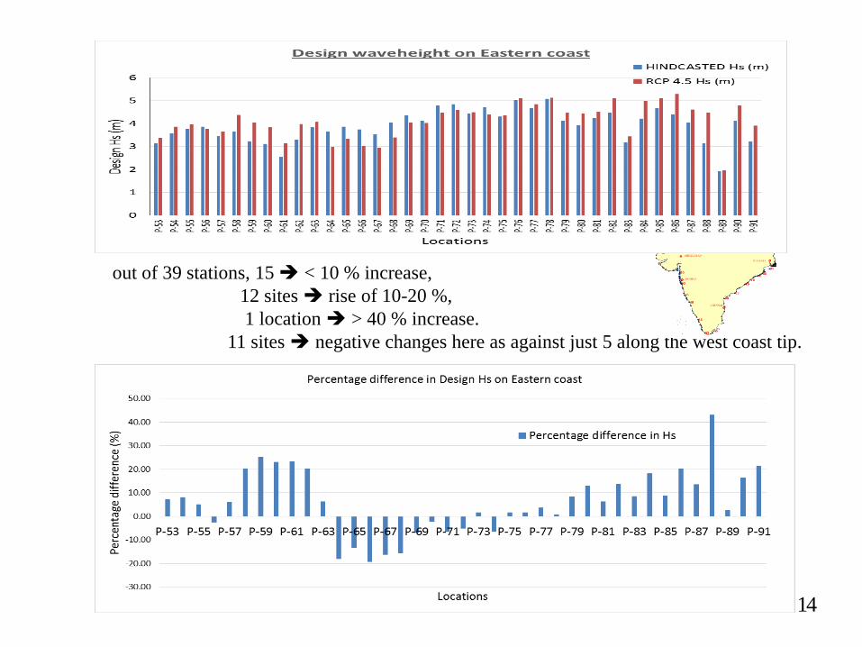
out of 39 stations, 15 < 10 % increase, 12 sites rise of 10-20 %, 1 location > 40 % increase. 11 sites negative changes here as against just 5 along the west coast tip.

14

• The future changes in Hs were highly site specific and non-uniform throughout the west or east coast.

• Reasons:

Site complexities. The sites at the southern tip of the coastline are subjected to complex wind

conditions because of exposure to AS, BoB and IO. The sites near entrances of gulfs, bays, river mouths, are affected by more

complex wave effects than open coasts.

• Reasons: The decrease can be due to local features: weaker wind circulation,

shifting of storms,… The increase in Hs could be due to the rise in wind and changes in

circulation as per some past studies at and around Indian seas. (Dobrynin et al., 2012, Bhaskaran et al., 2014, Satyavathi et al., 2016)

-Wind and waves in Southern Ocean will intensify in future sending swells northwards

(Dobrynin et al., 2015)

15

- In a separate work, Analysis of 15 CORDEX GCM winds was done at ~1400 grids mean wind will considerably increase in future until 2100. (CRPMP Project Report, 2017)

- In another study based on daily wind of 10 CMIP5 GCMs high wind may occur more frequently with change in directions in Arabian Sea and Bay of Bengal (Sumeet et al., 2015)

Reasons:

- Aboobacker et al., (2011) Intensification of ‘Shamal’ wind and swells coming from NE direction and from Persian Gulf in future.

16

-The observed rise in Hs is high compared with general global trends (Grabermann and Weisse, 2008).

- However local trend in Hs can be different than the global one -Mori et al., 2012, Wu et al., 2017, Dobrynin et al., 2015, Bennet et al., 2016).

At local level waves may build up because of changes in local topography, wind fetch and durations, wave directions and their frequencies of occurrence. -In this work a collective view of analysis of trends, pdf’s, wave roses point to the high rise in Hs.

17

Note:

Past works at or near the region of interest -Storms have intensified in northern Indian Ocean in past.

(Anoop et al., 2015) . - Annual mean Hs has shown rising trends in I O. (Hemer et al., 2010, Young et al., 2011, Shanas and Kumar, 2014).

-In recent decades higher waves occurred more frequently here. -(Patra and Bhaskaran (2016)

- The climate change signal in swells coming from Indian Ocean has been previously detected, distinguishing between climate variability and climate change . (Dobrynin et al., 2015)

18

-Past studies elsewhere

- An increase in the annual average wave heights ~ 0.022 m/yr off western England. (Carter and Draper, 1988)

-Hs with 100-year return were found be 10 % higher in North Sea (Reistad, 2001).

-In NE Atlantic- return periods of extreme waves may lower from 20 yr to ~12 to even 4 years. (Wang et al. 2004)

-In North Sea 7 % and 18 % increase in 99 percentile wind speed and Hs (Grabmann and Wiesse, 2008 )

-Maximum of 1.8 m rise in next 30 years along the U S east coast. - Komar and Allan (2008).

-Annual average Hs would grow by 0.015 m/yr while the annual extreme Hs would increase by 0.071 m/yr along the US NW Pacific. - Ruggiero et al. (2010)

19

Effect of changing

Ensemble RCM data by reanalysis data, and also,

Ensemble RCM data by single RCM data

for historical conditions

20

• In preceding work same type of wind data (RCM) were used for past and future for a meaningful comparison

21

Changing the wind input from ensemble RCM to reanalysis (ERA interim)

-27 coastal stations considered – same as study by India’s NIOT -30 years Hs data were considered (1985-2014 ). - GPD fitted at each site. 100-year Hs evaluated.

21

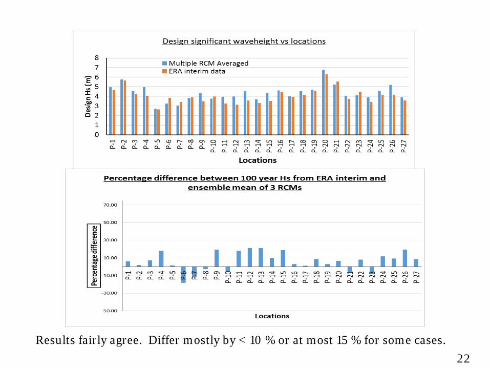
22 Results fairly agree. Differ mostly by < 10 % or at most 15 % for some cases.

22

Changing the wind input from ensemble RCM to a given single RCM

0

500

1000

1500

2000

P-1

P-2

P-3

P-4

P-5

P-6

P-7

P-8

P-9

P-10

P-11

P-12

P-13

P-14

P-15

P-16

P-17

P-18

P-19

P-20

P-21

P-22

P-23

P-24

P-25

P-26

P-27

P-28

P-29

P-30

P-31

P-32

P-33

P-34

P-35

P-36

P-37

P-38

P-39W

ater

Dep

th

(m)

Locations

23

24

Identical procedure was followed and 100-year Hs were derived based on historical data as per (i) single RCM and as per (ii) ensemble of RCM

Single RCM: RegCM4

24

Note: Larger difference

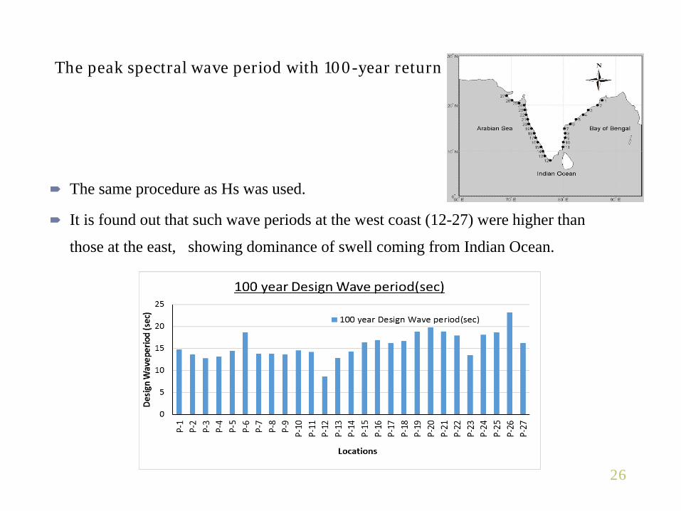
The same procedure as Hs was used.

It is found out that such wave periods at the west coast (12-27) were higher than

those at the east, showing dominance of swell coming from Indian Ocean.

The peak spectral wave period with 100-year return

25

The same procedure as Hs was used.

It is found out that such wave periods at the west coast (12-27) were higher than

those at the east, showing dominance of swell coming from Indian Ocean.

The peak spectral wave period with 100-year return

26

27 27

Conclusions The derivation of design Hs with 100-years’ return at a series of 91 locations along India’s west and east coasts generally indicated higher values when the basis of such derivation changed from past wave data to the projected one. The west coast showed relatively strong tendency of the design Hs to increase. At some locations however a decrease in the design Hs was also noticed. It is found that the changes were highly site specific and non-uniform throughout the west or east coastlines and those are most likely to be governed by local wind complexity and interaction with different met-ocean and geo-morphological factors. Considering changes in the probability density functions from past to future, the higher waves might appear more frequently and lower waves less frequently in future, indicating an intensified wave activity.

28 28

The wave rose diagrams prepared from past and projected waves showed that the west coast sites might see westward and east coast sites might experience eastward shift in the wave directions.

When the wind input to simulate waves was changed from the ensemble RCM

mean to a single RCM the differences were significantly large and hence the use of ensemble mean wind should be made in such studies for less uncertainty.

When the wind input was changed from the ensemble RCM to reanalysis

(ERA-Interim) wind, the differences were small indicating usefulness of the former wind type.

The values of the 100-year spectral peak wave period evaluated at various

locations showed that they were higher at the west coast than the east coast indicating the dominance of swells coming from the Indian Ocean.

It is suggested that future design of sea structures along the Indian coast may

consider possible changes in the design Hs as presented in this study.

29 29

30 30

0.0

50.0

100.0

150.0

1 2 3 4 5 6 7 8 9 101112131415161718192021222324252627

Dept

h (m

)

Location

National Institute of Ocean Technology, India published Wave Atlas (2014): Gives 50-yr Hs based on 15 years’ historical Hs data, derived from ERA-Interim wind, fitted to Weibull distribution using the total sample or full series method. It is generally agreed that GPD fitted using PoT is a better option considering required data independence. (Mathiessen et al., 1994)

We compared 100-year Hs derived from (i) GPD, PoT and (ii) Weibull dist., total sample, both based on 30-year ERA-Interim reanalysis wind.

31 31

0.0

2.0

4.0

6.0

8.0

1 2 3 4 5 6 7 8 9 10 11 12 13 14 15 16 17 18 19 20 21 22 23 24 25 26 27Hs

(m)

Location

Hs using Weibull Hs using GPD

-60-40-20

0204060

1 2 3 4 5 6 7 8 9 10 11 12 13 14 15 16 17 18 19 20 21 22 23 24 25 26 27Pe

rcen

tage

diff

eren

ce %

Location

(east coast: 1-11 west coast: 12-27)

- GPD-PoT produces much higher values than Weibull-full data over the east coast and opposite over the west coast. The reason: consideration of only high sea states (PoT) and fitting the dist. only to them, large number of cyclones. - Difference is small for the west coast, except at the extreme northerly sites -due to differences in fitting procedures. - Methods adopted for distribution fittings had more influence on the final outcome of design waves than that the choice of the driving wind at the specified locations. - Kolmogorov-Smirnov test - showed that at all the 27 locations such fit was not acceptable but at the same time the GPD fitted using PoT was statistically acceptable at all the sites.

32 32

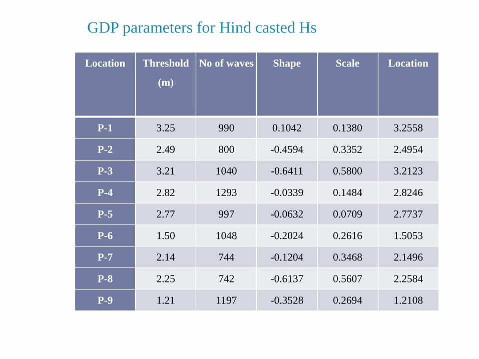
GDP parameters for Hind casted Hs

Location Threshold

(m)

No of waves Shape Scale Location

P-1 3.25 990 0.1042 0.1380 3.2558

P-2 2.49 800 -0.4594 0.3352 2.4954

P-3 3.21 1040 -0.6411 0.5800 3.2123

P-4 2.82 1293 -0.0339 0.1484 2.8246

P-5 2.77 997 -0.0632 0.0709 2.7737

P-6 1.50 1048 -0.2024 0.2616 1.5053

P-7 2.14 744 -0.1204 0.3468 2.1496

P-8 2.25 742 -0.6137 0.5607 2.2584

P-9 1.21 1197 -0.3528 0.2694 1.2108

33

Where

k = Shape factor, α = Scale factor β = Location Factor T = Return period λ = Mean rate

Generalized Pareto Distribution 34

35

Note: Although design life of a structure could be ~ 25 or so years, the design is based on 100 years’ climate (site-specific). Considering uncertainties in 100 years’ wave simulations, (interaction with changing met-ocean, geo-morpho. parameters, accounting of storms,…), the normal procedure to obtain design Hs involves considering ~ 30 years reliable simulations, fitting a theoretical distribution to it and, carrying out extrapolation to 100 years.