Evaluation Of

DIRECT PROPERTY TAX

RELI EF PROGRAMS

Office Of The Legislative Auditor Veterans Service Building St. Paul, Minnesota 55155

(612) 296-4708

February 4, 1983

 

PREFACE

In January 1982, the Legislative Audit Commission autho­rized the Office of the Legislative Auditor to study the state1s major direct property tax relief programs. From the study, we will issue two reports.

This report examines changes in the level of property tax over the past fifteen years and evaluates the effectiveness of the relief programs enacted when the Legislature concluded that property tax levels were too high. The report will show that the state1s complex set of property tax relief programs (direct and indirect) have brought Minnesota's residential property taxes down to their lowest point in recent years according to several relevant measures and a level lower than most other states. But the report will also show that these programs do not always target relief to those who need it the most. Without providing a detailed blueprint, the report attempts to point the way toward a more effective design of Minnesota's property tax relief system.

This part of our study was conducted by the Program Evaluation Division. Staff included Jim Nobles (Deputy Legislative Auditor for Program Evaluation), Elliot Long (Project Manager), Tom Walstrom, Dan Jacobson, and Rob Nevitt. We want to thank personnel f·rom the Departments of Revenue and Finance, staff from the Minnesota Senate and House of Representatives, and many others for supplying us with data and advice.

A second report, completed by the Financial Audit Division, will examine the administration of the state1s direct property relief programs. That report will be issued in approximately two weeks.

We are mindful that both reports address a complex set of problems that are not easily solved. But we are also hopeful that our analysis and recommendations will help in the very difficult decision­making that lies ahead. This report is solely the responsibility of the Office of the Legislative Auditor and does not necessarily represent the position of the Legislative Audit Commission or any of its members.

Gerald W. Christenson Legislative Auditor

 

I.

II.

TABLE OF CONTENTS

EXECUTIVE SUMMARY

A COMPARATIVE AND HISTORICAL REVIEW OF THE PROPERTY TAX AND PROPERTY TAX RELI EF IN MINNESOTA

A. Forms of Property Tax Relief B. Development of Property Tax Relief C. The Property Tax Burden in Minnesota D. Conclusion

GEOGRAPHIC VARIATION IN RESIDENTIAL PROPERTY TAXES

A. Causes of Geographic Variation B. Residential Property Taxes C. Property Taxes on Farm Homesteads

III. DIRECT PROPERTY TAX RELIEF PROGRAMS

IV.

V.

A. Homestead Credit B. Agricultural Credit C. Cumulative Effect of Direct Property Tax Credits D. Circuit Breaker E. Administration of the Circuit Breaker for Renters

(Renter's Credit)

PROPERTY TAX AND INCOME

A. Literature Review B. I ncidence of the Residential Property Tax C. Trends Over Time D. Over-All I ncidence of Property Tax Relief

Programs

POLICY OBJECTIVES IN THE STATE-LOCAL FISCAL RELATIONSHIP

A. Implications for Direct Property Tax Relief Programs

iii

ix

1

29

53

103

117

 

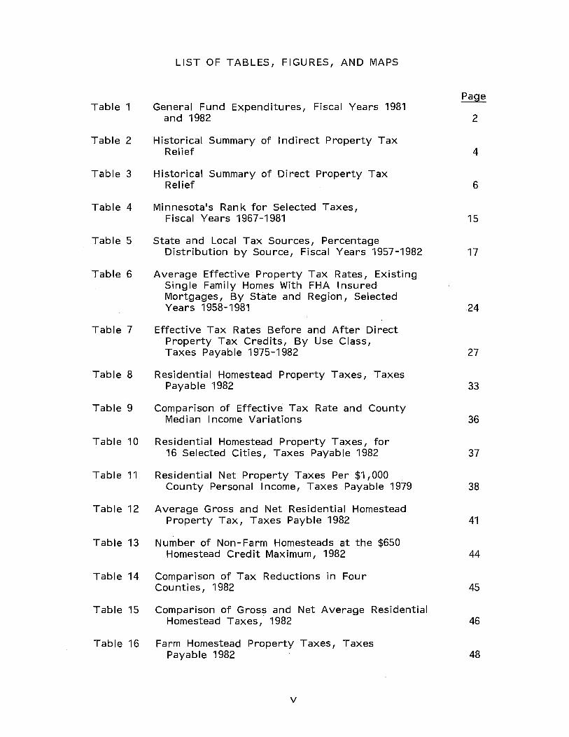
Table 1

Table 2

Table 3

Table 4

Table 5

Table 6

LIST OF TABLES, FIGURES, AND MAPS

General Fund Expenditures, Fiscal Years 1981 and 1982

Historical Summary of Indirect Property Tax Relief

Historical Summary of Direct Property Tax Relief

Minnesota's Rank for Selected Taxes, Fiscal Years 1967-1981

State and Local Tax Sources, Percentage Distribution by Source, Fiscal Years 1957-1982

Average Effective Property Tax Rates, Existing Single Family Homes With FHA Insured Mortgages, By State and Region, Selected Years 1958-1981

2

4

6

15

17

24

Table 7 Effective Tax Rates Before and After Direct Property Tax Credits, By Use Class, Taxes Payable 1975-1982 27

Table 8 Residential Homestead Property Taxes, Taxes Payable 1982 33

Table 9 Comparison of Effective Tax Rate and County Median I ncome Variations 36

Table 10 Residential Homestead Property Taxes, for 16 Selected Cities, Taxes Payable 1982 37

Table 11 Residential Net Property Taxes Per $1,000 County Personal Income, Taxes Payable 1979 38

Table 12 Average Gross and Net Residential Homestead Property Tax, Taxes Payble 1982 41

Table 13 Number of Non-Farm Homesteads at the $650 Homestead Credit Maximum, 1982 44

Table 14 Comparison of Tax Reductions in Four Cou nti es , 1982 45

Table 15 Comparison of Gross and Net Average Residential Homestead Taxes, 1982 46

Table 16 Farm Homestead Property Taxes, Taxes Payable 1982 48

v

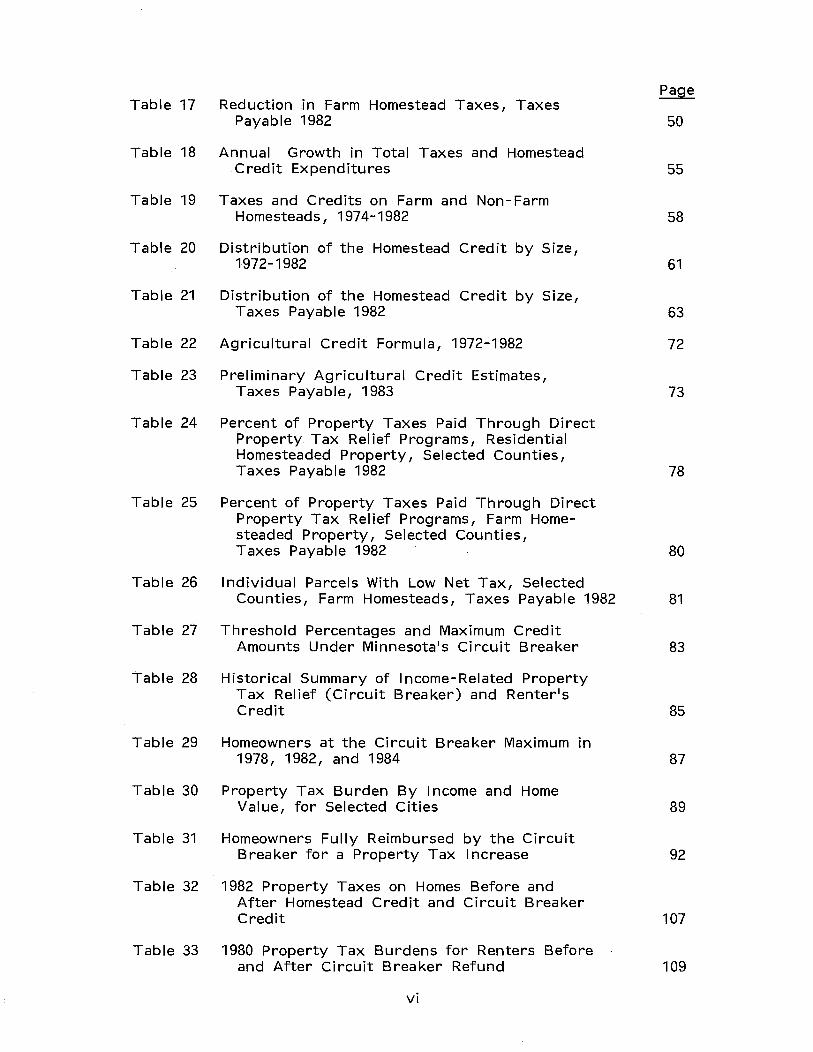
Table 17 Reduction in Farm Homestead Taxes, Taxes Payable 1982

Table 18 Annual Growth in Total Taxes and Homestead Credit Expenditures

Table 19 Taxes and Credits on Farm and Non-Farm Homesteads, 1974-1982

Table 20 Distribution of the Homestead Credit by Size, 1972-1982

Table 21 Distribution of the Homestead Credit by Size, Taxes Payable 1982

Table 22 Agricultural Credit Formula, 1972-1982

Table 23 Preliminary Agricultural Credit Estimates, Taxes Payable, 1983

Table 24 Percent of Property Taxes Paid Through Direct Property Tax Relief Programs, Residential Homesteaded Property, Selected Counties, Taxes Payable 1982

Table 25 Percent of Property Taxes Paid Through Direct Property Tax Relief Programs, Farm Home­steaded Property, Selected Counties, Taxes Payable 1982

Table 26 Individual Parcels With Low Net Tax, Selected Counties, Farm Homesteads, Taxes Payable 1982

Table 27 Threshold Percentages and Maximum Credit Amounts Under Minnesota1s Circuit Breaker

Table 28 Historical Summary of Income-Related Property Tax Relief (Circuit Breaker) and Renter1s Credit

Table 29 Homeowners at the Circuit Breaker Maximum in 1978, 1982, and 1984

Table 30 Property Tax Burden By Income and Home Value, for Selected Cities

Table 31 Homeowners Fully Reimbursed by the Circuit Breaker for a Property Tax Increase

Table 32 1982 Property Taxes on Homes Before and After Homestead Credit and Circuit Breaker Credit

Table 33 1980 Property Tax Burdens for Renters Before and After Circuit Breaker Refund

vi

50

55

58

61

63

72

73

78

80

81

83

85

87

89

92

107

109

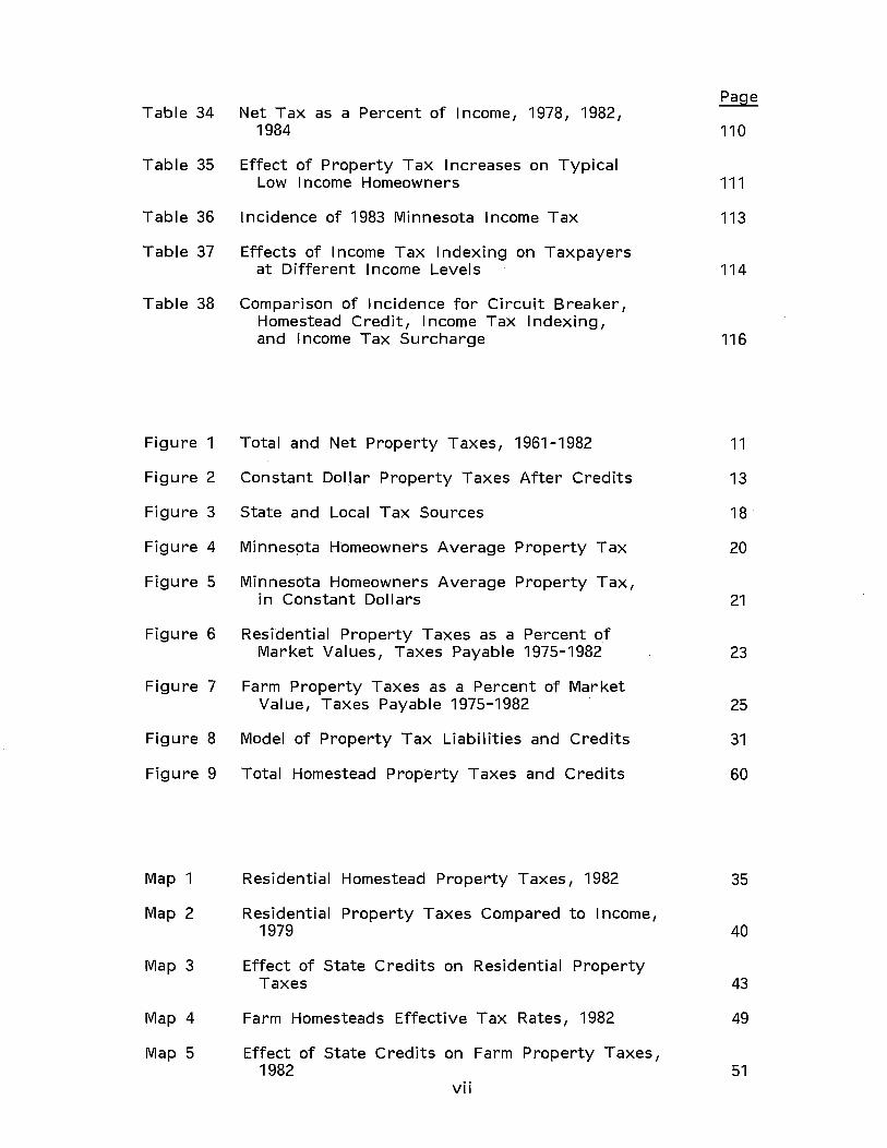
Table 34 Net Tax as a Percent of Income, 1978, 1982, 1984

Table 35 Effect of Property Tax I ncreases on Typical Low I ncome Homeowners

Table 36 Incidence of 1983 Minnesota Income Tax

Table 37 Effects of Income Tax Indexing on Taxpayers at Different I ncome Levels

Table 38 Comparison of I ncidence for Circuit Breaker, Homestead Credit, Income Tax Indexing, and Income Tax Surcharge

Figure 1 Total and Net Property Taxes, 1961-1982

Figure 2 Constant Dollar Property Taxes After Credits

Figure 3 State and Local Tax Sources

Figure 4 Minnespta Homeowners Average Property Tax

Figure 5 Minnesota Homeowners Average Property Tax, in Constant Dollars

Figure 6 Residential Property Taxes as a Percent of Market Values, Taxes Payable 1975-1982

Figure 7 Farm Property Taxes as a Percent of Market Value, Taxes Payable 1975-1982

Figure 8 Model of Property Tax Liabilities and Credits

Figure 9 Total Homestead Property Taxes and Credits

Map 1 Residential Homestead Property Taxes, 1982

Map 2 Residential Property Taxes Compared to Income, 1979

Map 3 Effect of State Credits on Residential Property Taxes

Map 4 Farm Homesteads Effective Tax Rates, 1982

Map 5 Effect of State Credits on Farm Property Taxes, 1982

vii

110

111

113

114

116

11

13

18

20

21

23

25

31

60

35

40

43

49

51

 

EXECUTIVE SUMMARY

Major property tax relief programs have been enacted and extended since 1967 in an effort to keep property taxes low, equalize the ability of communities across the state to raise revenue, and to help assure that low income property owners do not pay a dispropor­tionate amount of property tax. As much as three quarters of state tax revenue is returned to school districts and local units of govern­ment in order to substitute state for local revenue and reduce reliance on the property tax.

Many aspects of the state-local fiscal relationship currently merit study. This report focuses on one important part, direct property tax relief programs. These provide property tax relief directly to taxpayers--as in the case of the circuit breaker--or to local taxing districts on behalf of taxpayers--as in the case of the homestead credit. Not counting some late reductions and shifts expenditures through direct property tax relief programs now total over $786 million per year. The homestead credit, which pays 58 percent of the tax bill on homesteaded property to a $650 maximum, totalled about $479 million in 1982. The income adjusted property tax refund for homeowners and renters (circuit breaker) cost $168 million and the agricultural credit cost $87 million. These are the three major direct property tax relief programs and the principal focus of this report.

It is not an objective of th.is study to recommend whether or at what level direct property tax relief programs should be financed in Minnesota. However, we believe it is time to take a careful, even critical look at these (and other) property tax relief programs for these reasons:

• The state is short of money and needs to look to property tax relief programs for substantial savings.

Minnesota1s property tax system and system of aids and credits have grown to be the nation1s most complex. Better coordination of aids and credits and consolidation and simplification of the system is needed.

• There have been important changes in the property tax over the past 15 years. There is a real need for policy makers to review the present system and take stock of whether property taxes are high or low, and whether property tax relief programs are working as intended.

The common purpose of all direct property tax relief pro­grams is to keep property taxes (mainly residential property taxes) low. These programs are predicated on the belief that without direct property tax relief, Minnesota1s residential property taxes would be unacceptably high. Certainly, in 1967 when the homestead credit was enacted, and in 1971 when the reforms known as the Minnesota Miracle

ix

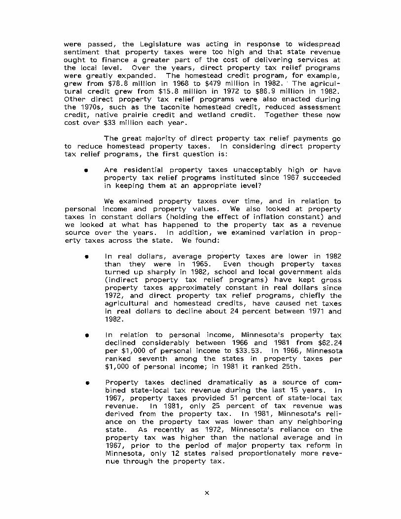
were passed, the Legislature was acting in response to widespread sentiment that property taxes were too high and that state revenue ought to finance a greater part of the cost of delivering services at the local level. Over the years, direct property tax relief programs were greatly expanded. The homestead credit program, for example, grew from $78.8 million in 1968 to $479 million in 1982. ' The agricul­tural credit grew from $15.8 million in 1972 to $86.9 million in 1982. Other direct property tax relief programs were also enacted during the 1970s, such as the taconite homestead credit, reduced assessment credit, native prairie credit and wetland credit. Together these now cost over $33 million each year.

The great majority of direct property tax relief payments go to reduce homestead property taxes. I n considering direct property tax relief programs, the first question is:

• Are residential property taxes unacceptably high or have property tax relief programs instituted since 1967 succeeded in keeping them at an appropriate level?

We examined property taxes over time, and in relation to personal income and property values. We also looked at property taxes in constant dollars (holding the effect of inflation constant) and we looked at what has happened to the property tax as a revenue source over the years. I n addition, we examined variation in prop­erty taxes across the state. We found:

• In real dollars, average property taxes are lower in 1982 than they were in 1965. Even though property taxes turned up sharply in 1982, school and local government aids (indirect property tax relief programs) have kept gross property taxes approximately constant in real dollars since 1972, and direct property tax relief programs, chiefly the agricultural and homestead credits, have caused net taxes in real dollars to decline about 24 percent between 1971 and 1982.

• I n relation to personal income, Minnesota's property tax declined considerably between 1966 and 1981 from $62.24 per $1,000 of personal income to $33.53. In 1966, Minnesota ranked seventh among the states in property taxes per $1,000 of personal income; in 1981 it ranked 25th.

• Property taxes declined dramatically as a source of com­bined state-local tax revenue during the last 15 years. In 1967, property taxes provided 51 percent of state-local tax revenue. In 1981, only 25 percent of tax revenue was derived from the property tax. In 1981, Minnesota's reli­ance on the property tax was lower, than any neighboring state. As recently as 1972, Minnesota's reliance on the property tax was higher than the national average and in 1967, prior to the period of major property tax reform in Minnesota, only 12 states raised proportionately more reve­nue through the property tax.

x

• Another way of looking at the property tax is to relate it to real estate values. Taxes as a percent of property value is called the effective tax rate (ETR). The effective tax rate for all property was about 4.0 in 1971. As a result of tax relief programs enacted that year and subsequently, effec­tive tax rates declined rapidly to 2.4 in 1975, 1.8 in 1978, and 1.2 in 1982. By 1982, property taxes as a percent of market value were about one-fourth of what they had been in 1971 and less than half of what they were in 1977.

• The effective tax rate on non-farm homesteads was 2.1 percent in 1975. Property taxes by this measure declined to 0.8 percent in 1981 and rose slightly to 1.0 percent in 1982. Farm owners' taxes show a similar pattern: a decline from 1.3 percent of market value in 1975 to 0.4 in 1981 and a rise to 0.5 percent in 1982.

• Minnesota has one of the nation's lowest effective tax rates on single family homes. A comparison among states using data on single family homes with FHA mortgages shows Minnesota's net property taxes to be 0.79 percent of market value in 1981. This is a lower tax rate than the effective tax rate in 42 other states. Outside the south only Ari­zona, Hawaii, and Wyoming have lower effective property tax rates on single family homes.

• Property taxes as a percent of market value on commercial property, apartments, public utilities and other classes not generally eligible for the homestead credit or other direct property tax relief payments have also declined significantly over the last seven years. For example, the effective tax rate on commercial property declined from 4.38 percent in 1975 to 2.83 percent in 1982. This of course reflects both increased aid to schools and local government but also increased property values.

I n short, Minnesota's property taxes are at an historically low level even after a sizeable upturn in 1982. Taxes on homesteaded property are especially low when compared to the past or in compari­son to other states. Minnesota's property tax relief programs have succeeded to a degree perhaps not widely appreciated.

Why isn't it generally understood that property taxes are relatively low in Minnesota?

• While property taxes have declined in relation to real estate values, personal income and the cost of living, because of inflation the average homeowner is in fact paying a larger property tax bill in 1982 than he paid in the mid 1970s. In 1975 the average property tax of Minnesota homeowners was $465; in 1982 it was $511.

• Property taxes turned up sharply in 1982 and are projected to increase over the next few years. Many homeowners are already receiving the maximum homestead and circuit breaker

xi

credits payable under current law and it is unreasonable to expect an increase in state funding of property tax relief sufficient to prevent residential property taxes from rising in the future.

• Perhaps the most important factor that helps to explain why homeowners feel that property taxes are high is that for some, taxes are high. While the statewide average property tax is low, over-all, taxes are especially low in some areas and relatively high in other areas.

Property taxes are highest in the Twin Cities metropolitan area and in other urban centers and relatively low in rural areas. Across the state, average 1982 property taxes on non-farm homes vary from $911.07 in Hennepin County to $114.81 in Itasca County. Every county in the Twin Cities metropolitan area has average taxes over $675, while half the counties in the state have average taxes that are under $256.

Property taxes vary across communities for a number of reasons:

• Urban areas require relatively high taxes to finance ser­vices which are characteristic of such communities and not found in rural areas.

• Taxes vary because of a concentration of people needing public services (such as children of school age or clients of public assistance programs) in some communities and not others.

• Taxes also vary because of expenses induced by rapid growth, differences in property wealth and the property mix across communities, differing preferences for public services, and other factors.

No effort has been made in this study to disentangle the separate contribution of each of these factors. The main point to keep in mind is that people are likely to regard property taxes as high or low, depending on where they live. Also, while the cost of housing varies significantly across the state, and while personal income also varies considerably, the variation in property taxes is even greater. Thus, property taxes as a percent of market value or personal income--measures which reflect property tax burdens--also vary widely across the state.

• For example, in 1982, Hennepin County residential home­steads paid an average of 1.2 percent of market value in property taxes while homesteads in Cook County paid 0.23 percent. This amounts to a 422 percent difference in property taxes from the highest to lowest county when market value is held constant.

xii

• Residential property taxes per $1,000 of personal income also vary widely across the state, from $21.21 per $1,000 of personal income in Hennepin County to $3.45 in Roseau County. (These figures are based on 1979 data, the last year for which income and property tax data can be matched. )

We examined the homestead credit, agricultural credit, and circuit breaker in some detail in order to learn how well the specific goals of each of these programs are being achieved.

HOMESTEAD CREDIT

The homestead credit is Minnesota·s largest direct property tax relief program. In 1982, the homestead credit reduced the prop­erty tax liability of homeowners by $479 million, although because of late cuts in the state funding the cost to the. state was reduced to $385 million for taxes payable in 1982.

The homestead credit became effective for taxes payable in 1968, and between 1968 and 1982 the amount paid through the home­stead credit grew by more than 500 percent. This increase is largely due to increases in the homestead credit limits enacted by the Legis­lature in 1973, 1979 and 1980.

• In 1968 the homestead credit paid 35 percent of homestead property taxes to a maximum of $250. In 1982 the credit paid 58 percent to a maximum of $650.

The homestead credit (excluding the taconite homestead credit) grew from $79 million in 1968 to $242 million in 1979, to $479 million in 1982. The cost of the program increased 54 percent in 1974, 46 percent in 1980, and 20 percent in 1981, reflecting the fact that increased benefits became effective each of those years.

• Payments through the homestead credit have grown more than twice as fast as tax levies between 1968 and 1982. The homestead credit grew faster than gross taxes on homesteads five of the six years between 1975 and 1981. As a result of the growth of the homestead credit, gross tax increases in 1975, 1976, and 1979 on homesteaded prop­erty actually became net tax decreases for homeowners.

Thus, it is clear that the homestead credit has succeeded in its primary purpose of keeping homeowners· property taxes low by substituting state for locally raised revenue.

The cost of the homestead credit will increase in the future unless the Legislature decides to change the terms of the program, because property tax levies can be safely predicted to go up and because nearly two-thirds of the homes in the state do not receive the maximum credit of $650. A reasonable projection is that the homestead credit will cost $513 million in 1983 and $532 million in 1984, unless the appropriation for the program is capped as it was in 1982.

xJii

There are more than a million homesteads in Minnesota and if all received the maximum credit of $650, the cost to the state would be about $670 million per year or 39.7 percent more than was actually obligated in 1982. Thus, if the 58 percent rate and $650 maximum are kept into the future, the growth in the cost of the homestead credit will be limited compared to increases experienced in recent years and the 500 percent increase since 1968.

The homestead credit is looked to by many to insulate homeowners from futu re property tax increases, perhaps becau se it worked this way during the 1970s, even to the point of causing a net tax decrease in certain years when gross taxes rose. However, unless the benefits of the program are increased for all or some taxpayers, and costs increased as well, the homestead credit will cease to protect increasing number of homeowners from the full effect of property tax increases. As fast as the homestead credit program has grown since 1968, in 1982 over a third of homesteads across Minnesota, over one-half in the Twin Cities metropolitan area and over 60 percent in Hennepin County received the maximum credit and are no longer insulated against property tax increases.

We conclude that the homestead credit is accomplishing what it was designed to do: Keep residential property taxes in Minnesota low. However, the state1s fiscal situation in 1983 and prospects for the near future are less promising than the conditions that prevailed through most of the 1970s when revenue growth driven by economic expansion and inflation permitted major increases in the homestead credit program.

It is debatable whether or not the homestead credit has made the Minnesota tax system more progressive. It should not be assumed that this is the case because state rev~nue sources that finance the homestead credit are not clearly more progressive than the property tax. And increases in the income tax due to inflation in the 1970s made the income tax less progressive, at the same time they financed increases in the homestead credit. By itself, the homestead credit has a slightly progressive effect on the property tax since it is capped at $650 and on the whole, upper income property owners receive a smaller percentage reduction in their property taxes than those with lower incomes. On the other hand, the $650 cap means that the homestead credit reduces taxes proportionately less in high tax areas such as the Twin Cities than in low tax areas, and actually works to increase the variation in taxes across the state.

Because the homestead credit provides a significant tax break to all Minnesota homeowners, it is not customary to discuss options that include reducing benefits paid through the program. Nevertheless, in light of the state1s fiscal situation in 1983 and pros­pects for the next few years, the homestead credit may be looked at as a program that should be redesigned. The homestead credit provides property tax relief broadly rather than concentrating relief in districts with low property wealth or a high level of service needs. Nor does the homestead credit distribute relief directly to taxpayers with high property taxes in relation to income. Alternatives to con­sider are essentially those presented by the school aid, local govern­ment aid and circuit breaker programs. Redirecting the funds now

xiv

provided through the homestead credit program makes the most sense when viewed as part of an effort to preserve the effectiveness of these programs. Options for the homestead credit include:

• Distributing all or part of the money now going to school districts and local government via the homestead credit through the school aid and local government aid programs.

• Distributing all or part of the homestead credit through the circuit breaker. I n effect this changes the homestead credit so that it is income sensitive.

• Reducing the homestead credit maximum, now $650, the homestead credit rate, now 58 percent, or both.

• Keeping the current rate and maximum, but exempting a minimum tax from the homestead credit.

We also have concluded that if the homestead credit is kept, the program, which represents 12 percent of annual general fund expenditures, should be administered with more precise and uniform standards and tighter controls. I n our judgement, at present it is very difficult for the state and local assessors to audit and verify homestead credit eligibility.

AGRICULTURAL CREDIT

The agricultural credit is designed to lower school taxes for the owners of agricultural property, timberland and non-commercial seasonal recreational property. These property owners are considered to be low users of school district services in relation to their share of property wealth within school districts and therefore deserve property tax relief.

The agricultural credit became a state-paid direct property tax relief program in 1972. Prior to 1972, the agricultural credit-­then computed as a mill rate, differential--was a local shift of school tax effort.

In 1982, nearly $87 million was paid to school districts on behalf of the owners of these classes of property and the cost of the agricultural credit is projected to reach $96 to $98 million in 1983. The agricultural credit has grown rapidly in cost between 1972 and 1982 from $16 million to $87 million. The cost of the agricultural credit doubled between 1978 when it was $35 million and 1981 when it cost $71 million.

The rapid increase in the cost of the agricultural credit is due to increases in the market value and assessed value of agricul­tural property and significant increases in the program's benefits.

• Statutory changes increasing the benefits paid through the agricultural credit program became effective in 1976 and each year between 1978 and 1982.

xv

As in the case of other direct property tax relief programs, we believe it is time to critically examine the agricultural credit in light of current conditions. The context of this examination is the same that guided our discussion of the homestead credit. The fiscal situation facing the Legislature in 1983 means that it is useful to examine alternatives that are aimed at saving· money or using existing resources more effectively.

The purpose, efficiency, and fairness of the agricultural credit can be questioned on several grounds:

• The agricultural credit provides about $87 million to school districts in a way that works at cross purposes to the state's foundation aid program.

The basic purpose of state school aid is to equalize the tax effort necessary to finance a basic level of education across the state. The agricultural credit is paid to rural school districts in direct proportion to property wealth, in contrast to the foundation aid program that distributes aid inversely to property wealth per pupil.

Historically, the state assumption of the cost of the agricul­tural credit was a compromise included in the entire package of reforms enacted in 1971, known as the Minnesota Miracle. The agri­cultural credit was extended during the 1970s in part because the foundation aid program was strengthened and it was considered appro­priate to compensate high-value agricultural districts which would not benefit from an increased foundation aid program.

• However, it may not be fully appreciated that the cost of the agricultural credit has grown about 450 percent since 1972. While the mandatory maintenance levy went down and back up during the last few years, the agricultural credit has been extended each year since 1978.

If the Legislature wants to reexamine the agricultural credit, a few additional problems are worth considering.

• Although it might be presumed that farms of equal value across the state receive an equal credit, the way the agri­cultural credit is designed means that small farms of given value receive a larger credit than large farms of the same value.

• Property in districts where assessed values are close to market values receives a higher agricultural credit than property in districts where assessments are low in compari­son to market values.

• Any homestead that sits on ten acres of land is classified as agricultural and thus qualifes for the agricultural credit. The agricultural credit is thus paid to many homesteads that by most definitions are not farms.

xvi

There are a number of basic and technical changes in the agricultural credit that we believe are worth considering.

• Redesign the agricultural credit to be more consistent with the foundation aid program and categorical aid programs that tie school aid to service needs and requirements and the ability of school districts to raise money.

• If the school tax burden on agricultural property, timber­land, and non-commercial seasonal recreational property is felt to be unfairly high, shift the tax effort within school districts through a locally paid credit or mill rate differ­ential.

• Adopt a more restrictive definition of what constitutes a farm for the purposes of paying the agricultural credit.

• Eliminate the inequality that is presently built into the agricultural credit that results in farms over 320 acres receiving a smaller credit than smaller farms of equal value.

CIRCUIT BREAKER

In 1981, homeowners received $54.1 million and renters received $114.2 million through the circuit breaker program that provides property tax relief to homeowners and renters based on property taxes or rent paid in relation to income.

The circuit breaker began in 1976, succeeding smaller rent credit and senior citizen property tax relief programs. The total cost of the program for homeowners and renters grew from $121.7 million in 1976 to $195.2 million in 1978, then declined to $168.3 million in 1981.

• Circuit breaker benfits for homeowners declined when the homestead credit was increased in 1979 and 1980 because there is a dollar for dollar substitution between these programs for many homeowners.

(

• Estimates for 1982 and projections for 1983 and 1984 indicate that the circuit breaker will reverse its downward trend and grow to $219 million in 1984. These projections reflect the significant rise in property taxes in 1982, the expecta­tion that taxes will continue to rise, and assume no change in the terms· of the homestead credit and circuit breaker programs. If the homestead credit is reduced, the cost of the circuit breaker will rise.

To determine how well the circuit breaker is working and to identify how its design can be improved, we analyzed how well it achieves its objectives and reviewed criticisms of the circuit breaker made in the public finance literature. The circuit breaker has three major purposes.

xvii

• To make the property tax more progressive;

• To compensate renters for tax breaks received by home­owners through the homestead credit and income tax breaks;

• To relieve hig/1 property tax burdens relative to income for low and middle income households.

We found:

• Minnesota's property tax relief programs, particularly the circuit breaker, make Minnesota's property tax nearly proportional for homeowners and progressive for renters. Thus the circuit breaker is effective both in making the property tax more progressive and in providing additional aid for renters.

However, the circuit breaker is becoming less effective at relieving high tax burdens relative to income because more homeowners are reaching the income limits or the maximum credit. As result, by 1984, the circuit breaker will not be very sensitive to income or taxes in the Twin Cities metropolitan area and other high tax areas. For example, we found:

• In the Twin Cities metropolitan area and other high tax areas, nearly one-half of homeowners with incomes less than $33,000 will be at the circuit breaker maximum by 1984. As a result, the circuit breaker will soon give the same credit to homeowners who have high property taxes as it does to homeowners at the same income level who have average property taxes.

• All senior citizens and disabled persons whose gross prop­erty taxes exceed $1,450 will receive the same maximum credit of $1,000 regardless of whether their income is $20,000 or less than $5,000. The same situation exists for homeowners under 65 if thei r g ross taxes exceed $1,650. By 1984, many senior citizens in the Twin Cities metropol­itan area and other high tax areas will be in this situation. If gross property taxes increase by 25 percent between 1982 and 1984, gross taxes on homes in Minneapolis or St. Paul worth more than $68,000 will exceed $1,450.

• While family incomes have increased rapidly since the circuit breaker began in 1976, the circuit breaker's effective income limit for homeowners under 65 has declined from $36,000 to $33,000. As a result, many middle income home­owners are no longer eligible for a circuit breaker refund.

There are several alternatives which can improve the design of the circuit breaker. These include:

• Reduce the circuit breaker's 100 percent credit rate.

• Raise the circuit breaker's maximum credit amounts.

xviii

• I ncrease the circuit breaker1s income brackets.

• Change to a sliding scale formula.

These options have the following advantages.

The options which increase the maximum credit and/or reduce credit rates will reduce the number of homeowners who are at the circuit breaker maximum credit and thus more effectively target property tax relief to homeowners with high taxes relative to their income.

Increasing income brackets can ensure that middle income homeowners do not become ineligible simply because their incomes have increased with inflation.

I n addition, reducing the 100 percent credit rate ensures that homeowners pay at least a part of any property tax increase and thus may reduce the incentive for local governments to spend exces­sively. Because of this change, the circuit breaker would also more uniformly relate property taxes to house value and level of local services. Currently, nearly two-thirds of homeowners eligible for the circuit breaker will either pay the full burden of a property tax increase because they are at the maximum or pay none at all. Re­ducing the number of homeowners at these extremes would make the circuit breaker more equitable. This could be particularly important if the homestead credit were substantially reduced because more homeowners would be eligible for the circuit breaker and the number of homeowners who would be fully reimbursed for a property tax increase could rise substantially.

These changes will not necessarily increase the cost of the circuit breaker because cost savings from reducing the 100 percent credit rate can offset the additional cost of raising the maximum credits and income brackets. Another option which can have similar advantages as the options discussed above is the sliding scale for­mula, under which the credit equals a percentage of tax where the percentage decl i nes as income increases.

One possible disadvantage of making these changes is that some homeowners will lose benefits. At a time when property taxes are rising rapidly, this may appear to place an unacceptable burden on these taxpayers. However, the homeowners who would lose the most from this change are those for whom the circuit breaker now rebates 100 percent of a property tax increase. By reducing benefits for these homeowners and raising benefits for homeowners at the maximum, tax increases can be distributed more evenly than they would be under the current circuit breaker.

We also examined the administration of the circuit breaker for renters and found that taxpayers I statements of rent paid are extremely difficult to verify and audit on a cost-effective basis. Our own extensive study of a sample of 560 claims suggests that in 1981, the state should have paid $104.5 million through the renter1s credit rather than the $118.7 million actually paid.

xix

POLICY OBJECTIVES IN THE STATE-LOCAL FISCAL RELATIONSHIP

We believe that direct property tax relief programs need to be deliberated in the context of the entire state-local fiscal relation­ship. A number of general principles have been advanced by various groups as a basis for reforming the state-local fiscal system. Those with broad support that we endorse as well include the following:

• Minnesota1s state-local fiscal system needs comprehensive reform.

• Greater predictability and stability in state aid is needed by local government.

• The system as a whole including the property tax system should be simplified in order to promote understanding, reduce record-keeping costs, and promote uniform classifi­cation and assessment practices across the state.

• Many of the objectives of Minnesota1s complex property classification and tax relief system could be better achieved through budgeted expenditures.

• State· aid to local government should neither encourage nor discourage local spending. State aid should not provide cheap marginal dollars in support of local levies.

• While often maligned, the property tax is essential because it taxe's a form of wealth that would otherwise go untaxed, and it is the only significant tax available to local govern­ment.

• Local government is best equipped to deliver a wide range of public services, while equity in taxing and spending dictates that the state carry a major part of the responsi­bility for financing those services. I n order to assure that local government is effective, efficient and fair, local gov­ernment needs a large measure of autonomy in spending decisions, and the ability to raise revenue adequate to finance services demanded, through the political process, by local residents.

• The over-all effect of state and local taxing and spending programs should be progressive. Individual taxes or spend­ing programs need not pass this test, although it is an important criterion on which they should be judged.

In judging direct property tax relief programs against these criteria we conclude that:

• The homestead credit can be criticized because it makes cheap dollars available to local taxing districts and can thus encourage a higher local property tax than would otherwise be approved. The circuit breaker for homeowners as now designed can have this effect as well.

xx

• Direct property tax relief programs are not the most com­plicated aspect of the property tax system. Even so, these programs can combine in ways that the legislature presum­ably did not intend. For example, some individual parcels of property of substantial value pay either no property tax or very little tax because of the additive effects of individual programs.

• There are costly administrative problems at the local level connected with the homestead and agricultural credits.

• It is questionable whether direct property tax relief pro­grams other than the circuit breaker have a progressive impact on the Minnesota tax system.

Property tax relief has been an issue of singular importance in Minnesota over the last 15 years. It is not less important in 1983. This report is offered as a source of information that will help policy makers first understand a complex system, then decide what changes need to be made.

xxi

 

I. A COMPARATIVE AND HISTORICAL REVIEW OF THE PROPERTY TAX AND PROPERTY TAX RELIEF IN MINNESOTA

This chapter presents an overview of the property tax and property tax relief programs in Minnesota. The first section de­scribes Minnesota1s property tax relief programs and their costs. The next section reviews the historical factors that gave rise to the enactment of these programs. In the final section we analyze Minne­sota1s property tax levels over time and in comparison with other states. Essentially we ask: What is the property tax burden in Minnesota? How successful is the state1s effort to reduce reliance on the property tax? The answers will form the basis for the critical analysis of the state1s direct property tax relief programs that follows.

A. FORMS OF PROPERTY TAX RELI EF

Although the focus of our report is direct property tax re­lief J it is important to recognize that Minnesota provides property tax relief through a number of programs that transfer state revenue to local governments and individuals. We have divided these transfers into two broad categories: indi rect property tax relief, such as school and local government aids that are paid by the state to local units prior to calculation of local levies, thus holding down the amount that must be levied; and direct property tax relief programs, such as the homestead credit and agricultural credit that reduce the tax bill received by individual property owners. Under these programs, the state pays to local taxing units a share of the gross tax liability on behalf of the property taxpayer. The state also provides direct property tax relief through refund programs, such as the circuit breaker for homeowners and renters. These rffund programs are administered through the state income tax system.

I n fiscal years 1981 and 1982, almost 62 percent of state collected tax revenues were returned to local governments and indi­viduals under the programs we have categorized as indirect and direct property tax relief. Table 1 presents a broad view of how the state1s general fund was distributed in the last two fiscal years. As Table 1 shows, over 55 percent of the state1s general fund expendi­tures were returned to local governments.

1The reader needs to be cautioned that some reports refer to programs such as school aids and local government aids as IIdirect aid, II meaning they are paid directly to governmental units. We refer to these as indirect property tax relief because they are not tied directly to individual parcels of property and are typically designed to support general government functions and services. I n contrast, the programs we have characterized as direct property tax relief are tied directly to individual parcels of property and result either in a credit paid by the state on behalf of a property owner or a tax refund to an individual.

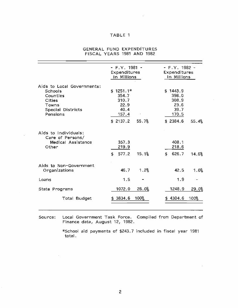
TABLE 1

GENERAL FUND EXPENDITURES FISCAL YEARS 1981 AND 1982

Aids to Local Governments: Schools Counties Cities Towns Special Districts Pensions

Aids to Individuals: Care of Persons/

Medical Assistance Other

Aids to Non-Government Organizations

Loans

State Programs

Total Budget

- F. Y. 1981 -Expenditures

I n Millions

$ 1251.1* 354.7 310.7

22.9 40.4

157.4

$ 2137.2 55.7%

357.3 219.9

$ 577.2 15.1%

46.7 1.2%

1.5

1072.0 28.0%

$ 3834.6 100%

- F. Y. 1982 -Expenditures

I n Millions

$ 1443.9 398.0 308.9

23.6 39.7

170.5

$ 2384.6 55.4%

408.1 218.6

$ 626.7 14.6%

42.5 1.0%

1.9

1248.9 29.0%

$ 4304.6 100%

Source: Local Government Task Force. Compiled from Department of Finance data, August 12, 1982.

*School aid payments of $243.7 included in fiscal year 1981 total.

2

1. INDIRECT PROPERTY TAX RELIEF PROGRAMS

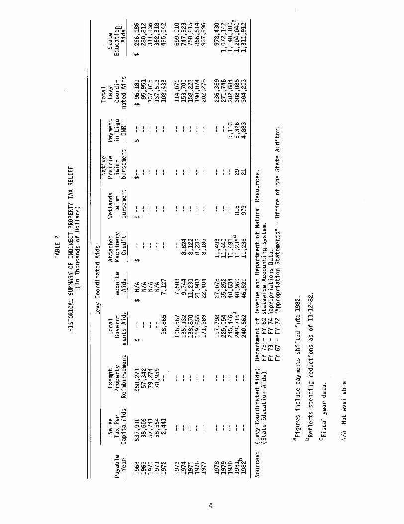
All state aids to schools and local governments can be con­sidered property tax relief because they replace dollars that, given a fixed level of local spending, would otherwise be raised through local property taxes. Table 2 presents a picture of how the major types of indirect property tax relief programs have changed and grown since 1968.

As Table 2 shows, the major form of indirect property tax relief is the education aid system. Historically, Minnesota funded schools through a locally imposed property tax. Over time, property taxes were supplemented by limited state aids. I n1971, the Legis­lature enacted a school aid system that substantially increased the amount of equalized foundation aid to school districts while imposing a limitation on the property tax rate for schools. The foundation aid program is designed to provide relati'iely more aid to districts with lower property wealth per pupil unit. I n general, levy limits are designed to hold down increases in school district and other local government levies and thus to assure that state education and other aids in fact are translated into property tax relief. Over $1.3 billion in various education aids was provided in 1982.

The local government aid program was enacted in 1971 for the general support of local government operations. Counties, cities, and towns receive aid based on a statutory formula. In 1982, approx­imately $240 million in local government aid was distributed. In addition, an attached machinery credit distributes reimbursements each year to school districts, county, city, and town governments for the revenue lost due to exemption of machinery and equipment from the property tax. In 1982, attached machinery aid amounted to $11.2 million.

2. DI RECT PROPERTY TAX RELI EF PROGRAMS

Under our categorization, direct property tax relief pro­grams are those tied directly to individual parcels of property and result either in a credit paid by the state to local governments on behalf of property owners or a tax refund to an individual. These direct property tax relief programs are:

• Homestead Credit

• Circuit Breaker for Homeowners and Renters

• Agricultural School Credit

• Taconite Homestead Credit

1The state education aid system is much more complex than presented here. In addition to foundation aids, the state pays trans­portation aid, vocational education aids, and a variety of other aids. For a more detailed discussion, see Minnesota School Finance, Minne­sota House Research Department, November, 1982.

3

Pay

able

Y

ear

1968

19

69

1970

19

71

1972

1973

19

74

1975

19

76

1977

+

»

1978

19

79

1980

19

81b

1982

Sou

rces

:

Sal

es

Exem

pt

Tax

Per

P

rope

rty

TABL

E 2

HIS

TORI

CAL

SUM

MAR

Y OF

IN

DIR

ECT

PROP

ERTY

TAX

RE

LIEF

(I

n T

hous

ands

of

Do

llar

s)

Lev~

Coo

rdin

ated

Aid

s N

ativ

e L

ocal

A

ttac

hed

Wet

land

s P

rair

ie

Gov

ern-

Tac

onit

e M

achi

nery

R

eim

-R

eim

-C

aEit

a A

ids

Rei

mbu

rsem

ent

men

ts

Aid

s A

ids

Cre

dit

burs

emen

t bu

rsem

ent

$37,

910

$58,

271

$ $

N/A

$

$ --

$--

38,6

09

57,3

42

N/A

57

,741

79

,274

N

/A

58~554

78,9

59

N/A

2,

441

98,8

65

7,12

7

106,

567

7,50

3 13

5,13

2 9,

744

8,82

4 13

8,87

0 11

,231

8,

122

159,

855

21,9

83

8,23

6 17

1,68

9 22

,404

8,

185

197,

798

27,0

78

11,4

93

225,

054

35,2

52

11,4

40

245,

446

40,6

34

11,4

91a

249,

716

a 40

,960

11

,238

81

6 29

24

0,56

2 46

,520

11

,238

97

9 21

(Lev

y C

oord

inat

ed A

ids)

D

epar

tmen

t o

f R

even

ue a

nd D

epar

tmen

t o

f N

atur

al

Res

ourc

es.

(Sta

te E

duca

tion

Aid

s)

FY 7

5 -

FY 8

2 S

tate

wid

e A

ccou

ntin

g Sy

stem

. FY

73

-FY

74

App

ropr

iati

ons

Dat

a.

Paym

ent

in L

i~u

DNR

$ 5,11

3 5,

326

4,88

3

FY 6

7 -

FY 7

2 II

App

ropr

iati

on S

tate

men

ts II

-O

ffic

e o

f th

e S

tate

Aud

itor

.

aFig

ures

in

clud

e pa

ymen

ts

shif

ted

in

to 1

982.

bRef

lect

s sp

endi

ng r

educ

tion

s as

of

11-1

2-82

.

cFis

cal

year

dat

a.

N/A

N

ot A

vail

able

Tot

al

Levy

S

tate

C

oord

i-E

duca

tion

na

ted

Aid

s A

idsc

$ 96

,181

$

266,

186

95,9

51

280,

812

137,

015

311,

136

137,

513

352,

318

108,

433

495,

042

114,

070

699,

010

153,

700

747,

923

158,

223

758,

615

190,

074

856,

814

202,

278

937,

996

236,

369

978,

430

271,

746

1,07

2,14

2 30

2,68

4 1,

148,

100 a

308,

085

1,20

4,04

0 30

4,20

3 1,

311,

912

• Reduced Assessment Credit

• Wetlands Credit

• Native Prairie Credit

• Power Line Credit

• Disaster Relief Credit

I n this section we briefly describe each direct property tax relief program. The major programs will be described more fully in later chapters of this report.

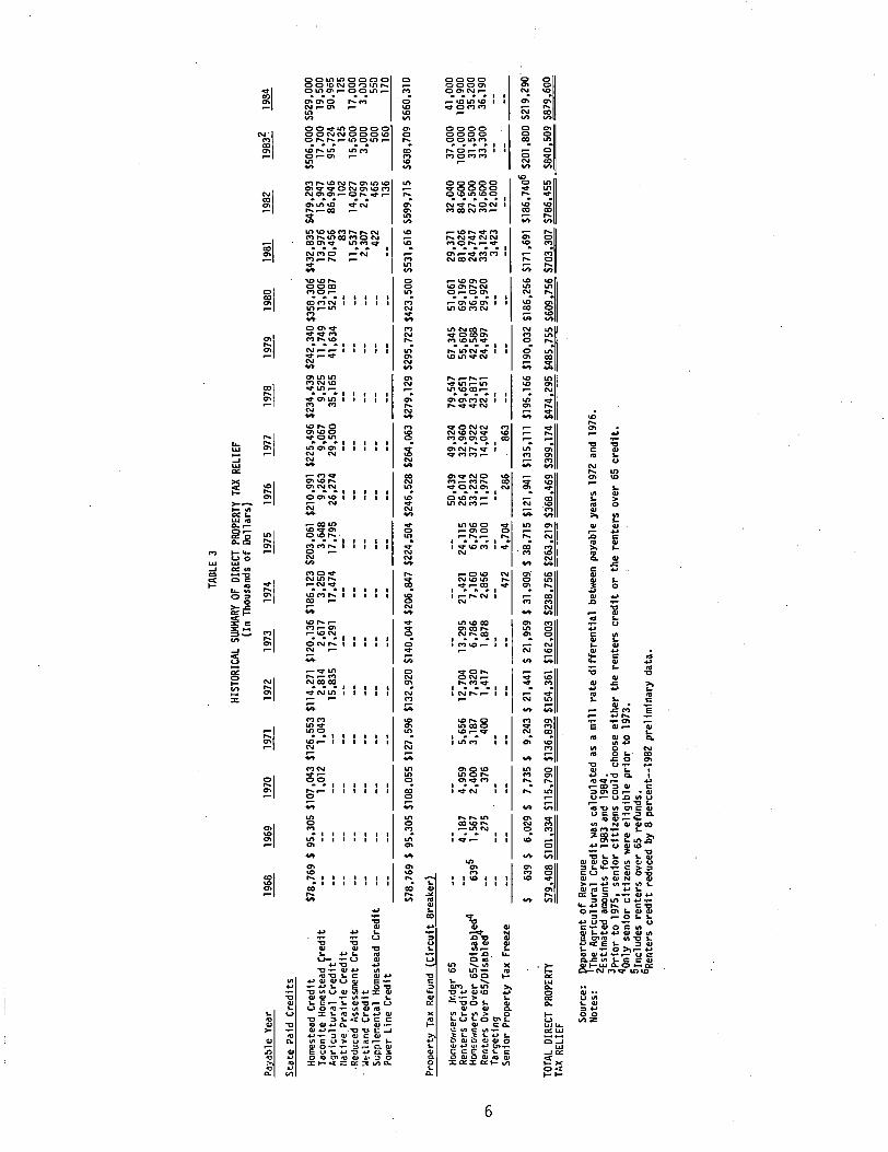
Table 3 shows that property tax relief through direct property tax relief programs, principally the homestead credit, agri­cultural credit, and circuit breaker has grown four-fold between 1973 and 1982, from $162 to $786 million. The principal component of this growth has been the homestead credit. The homestead credit was enacted in 1967 anp provides a direct reduction of tax for all home­steaded property. The percentage reduction has been increased several times over the years and is currently 58 percent, up to a maximum credit of $650. For farm homesteads the tax on the home plus 240 acres is eligible for reduction. The state reimburses local governmental units for the loss of revenue represented by the credit reduction on the tax bill. The homestead credit is paid to school districts and other taxing districts in proportion to the size of the tax levy of each taxing district in which a homestead is located. Table 3 shows that homestead property tax bills were reduced by $479 million in 1982. Because of budgetary shortfalls, the state has not reimbursed local governments for the full amount that property tax bills were reduced. For taxes payable in 1982, the state will actually pay approximately $385 million to local governments. Under the provisions of current law, it is estimated that the homestead credit will cost $506 million for taxes payable in 1983 and $529 million for taxes payable in 1984. The homestead credit program is treated in detail in Chapter 3 of this report.

The second major type of direct property tax relief is the property tax refund or circuit breaker program. This program provides homeowners and renters with an income tax credit or refund based on the amount of property tax paid in relation to income. Homeowners are eligible for this program when their property taxes exceed a specified percentage of household income ranging from .5 percent for incomes less than $3,000 to 4 percent for incomes over $100,000. Renters become eligible in the same way except they count 23 percent of their rent (excluding utilities) as property tax.

Of the two circuit breaker programs, only the renters credit has grown significantly in recent years. Expenditures through

1 Eligibility for the homestead credit is determined by the assessor1s classification of a property. Most generally, homesteaded property is that owned and occupied on January 2 as a place of primary residence.

5

m

Paya

ble

Yea

r

Sta

te P

aid

Cre

dits

Hom

este

ad C

redi

t T

acon

ite H

omes

tead

~redit

Agr

icul

tura

l C

redi

t fl

ativ

e P

rair

ie C

redi

t .R

educ

ed A

sses

smen

t C

redi

t )/<

:tlan

d C

redi

t Supp1e~ental

Hom

este

ad C

redi

t Po

wer

Lin

e C

redi

t

1968

19

69

1970

19

71

TABL

E 3

HIST

ORIC

AL S

UMMA

RY O

F DI

RECT

PRO

PERT

Y TA

X RE

LIEF

(I

n Th

ousa

nds

of

Dol

lars

)

1972

19

73

1974

19

75

1976

19

77

1978

19

7!!,

1980

19

81

1982

$78,

769

$ 95

,305

$10

7,04

3 $1

26,5

53 $

114,

271

$120

,136

$18

6,12

3 $2

03,0

61

$210

,991

$2

25,4

96 $

234,

439

$242

,340

$35

8,30

6 $4

32,8

35 $

479,

293

1,01

2 1,

043

2,81

4 2,

617

3,25

0 3,

648

9,26

3 9,

067

9,52

5 11

,749

13

,006

13

,976

15

,947

15

,835

17

,291

17

,474

17

,795

26

,274

29

,500

35

,165

41

,634

52

,187

70

,456

86

,946

83

10

2 11

,537

14

,027

2,

307

2,79

9 42

2 46

5 13

6

1983

2 19

84

$506

,000

$52

9,00

0 17

,700

19

,500

95

,724

90

,965

12

5 12

5 15

,500

17

,000

3,

000

3,0,

)0

500

550

_--!

.:16

~0 -

-1Z

.Q.

S78,

769

$ 95

,305

$10

8,05

5 $1

27,5

96 $

132,

920

$140

,044

$20

6,84

7 $2

24,5

04 $

246,

528

$264

,063

$27

9,12

9 $2

95,7

23 $

423,

500

$531

,616

$59

9,71

5 $6

38,7

09 $

660,

310

Pro

pert

y Ta

x R

efun

d (C

ircu

it 8

reak

er)

Hon

E;lJ'

"ner

s Jr

.djr

65

Ren

ters

Cre

dit

Hon~

owne

rs O

ver

65/0

iSab

!ed

4 R

ente

rs O

ver

65/0

isab

led

Tar

geti

ng

. S

enio

r P

rope

rty

Tax

Free

ze

6395

4,

187

1,56

7 27

5

4,95

9 2,

400

376

5,65

6 3,

187

400

12,7

04

7,32

0 1,

417

13,2

95

6,78

6 1,

878

21,4

21

7,16

0 2,

856

24,1

15

6,79

6 3,

100

50,4

39

26,0

14

33,2

32

11,9

70

49,3

24

32,9

60

37,9

22

14,0

42

79,5

47

49,6

51

43,8

17

22,1

51

67,3

45

55,6

02

42,5

88

24,4

97

51,0

61

69,1

96

36,0

79

29,9

20

29,3

71

81,0

26

24,7

47

33,1

24

3,42

3

32,0

40

84,6

00

27,5

00

30,6

00

12,0

00

~~ _

_ .-::

..::

.._~

::..

:...

.-_

__

_ ~:

:..:

....

-__

_ 4:!,!

7.!:,2

4,70

4 28

6 86

3 _

__

__

__

__

_ -=

__

_ _

37,0

00

41,0

00

100,

000

106,

900

31,5

00

35,2

00

33,3

00

36,1

90

TOTA

L DI

RECT

PRO

PERT

Y TA

X RE

LIEF

$ 63

9 $

6,02

9 $

7,73

5 $

9,24

3 $

21,4

41

$ 21

,959

$ 3

1,90

9 $

38,7

15 $

121,

941

$135

,111

$1

95,1

66 $

190,

032

$186

,256

$17

1,69

1 $1

86,7

406

$201

,800

$21

9,29

0'

$79,

408

$101

,334

Sl1

5,79

0 $1

36,8

39 $

154,

361

$162

,003

$23

8,75

6 $2

63,2

19 $

368,

469

$399

,174

$47

4,29

5 $4

85,7

55 $

609,

756

$703

,307

$78

6,45

5 S8

40,5

09 ~

Sour

ce:

Not

es:

Dep

artm

ent

of

Rev

enue

~The

Agr

icul

tura

l C

redi

t w

as c

alcu

late

d as

a m

ill

rate

dif

fere

nti

al b

etw

een

paya

ble

year

s 19

72 a

nd 1

976.

E

stim

ated

am

ount

s fo

r 19

83 a

nd

1984

. :p

rio

r to

197

5,

seni

or c

itiz

~ns

coul

d ch

oose

eit

her

the

ren

ters

cre

dit

or

the

rent

ers

over

65

cred

it.

Onl

y se

nior

cit

izen

s w

ere

elig

ible

pri

or

to 1

973.

5I

nclu

des

rent

ers

over

65

refu

nds.

6R

ente

rs c

red

it r

educ

ed b

y 8

perc

ent-

-198

2 pr

elim

inar

y da

t~.

the circuit breaker for homeowners have declined. This has occurred because incomes have increased faster than net property taxes and because of the rapid expansion of the homestead credit and other direct credits. In 1981, homeowners received $54.1 million and renters received $114.2 million from the circuit breaker programs. In ·1984, according to Department of Revenue projections, homeowners will receive $76 million and renters will receive $143 million. The circuit breaker will be discussed more fully in Chapter 3.

Targeted relief is a program that provides a refund to homeowners whose net taxes have increased sharply. Targeted relief is based simply on an increase in net taxes and is not adjusted ac­cording to household income like the other property tax refunds. Targeted relief was paid in 1981 and 1982. Although the program is still in law, no money has been appropriated for future years.

The agricultural credit became a state paid credit in 1971. The agricultural credit is paid to school districts to reimburse them for the reduction of taxes on specified property classes. The agri­cultural credit is designed to reduce the portion of taxes that owners of agricultural, noncommercial seasonal recreation, and timber prop­erty pay for schools. For agricultural homesteads, the credit is equal to the sum of 18 mills times the assessed value of the first 320 acres, 10 mills times the assessed value of the next 320 acres, and 8 mills times the assessed value of any acreage over 640 acres. Non­homesteaded agricultural property taxes are reduced by the sum of 10 mills times the assessed value of the first 320 acres and 8 mills times the assessed value of any acreage over 320 acres. Non-commercial seasonal recreation property taxes are reduced by an amount equal to 10 mills times the assessed value. Timber property taxes are reduced by an amount equal to 8 mills times the assessed value.

In 1982, almost $87 million was provided to school districts through the agriculture credit. The program is projected by the Department of Revenue to cost $95.7 million in 1983 and $91.0 million in 1984. A discussion of the agricultural credit1s purpose and an evaluation of its effectiveness is included in Chapter 3.

I n addition to these major direct property tax relief pro­grams there are several other programs that serve more limited pur­poses. The state pays taconite homestead, reduced assessment, wetlands, native prairie, power line and disaster relief credits to compensate local governments for tax relief given to individuals by these state programs. Together these other credits accounted for $33.5 million, or about 4.3 percent, of the $786 million in direct property tax relief for taxes payable in 1982. Because they account for such a small portion of property tax relief they are not discussed in detail in this report, although they are referred to from time to time. Nonetheless, these credits are important components of prop­erty tax relief for individual groups of taxpayers, and as such they are described briefly below.

7

The taconite ho~estead credit 1 and the supplemental home­stead property tax relief programs provide property tax relief to homesteaded property in taxing districts where taconite facilities are located. In 1982, homesteaded residential property and 240 acres of farm homesteaded property are eligible for, depending on the taxing district, either a 66 percent reduction in gross taxes not to exceed $445 or a 57 percent reduction not to exceed $380. These maximums go up automatically $15 per year. The taconite homestead credit is paid from a dedicated portion of the taconite production tax, not from the general fund. Because of the decreased production of taconite, annual payments from the taconite property tax relief fund are cur­rently exceeding annual receipts. The fund is expected to be in deficit beginning in 1985.

The reduced assessment credit3 was enacted in 1980 and first paid in 1982. The purpose of the credit is to provide a replace­ment for revenue lost to local governments from the preferential assessment of the homesteaded property of the blind and disabled, and of the housing structures for low income or elderly citizens financed through the Farmers Home Administration, Minnesota Housing Finance Agency, or under Title II of the National Housing Act. The credit is intended to eliminate the shift in tax burden to other classes of property within a taxing district that would otherwise result from preferential assessment. For taxes payable in 1982, the program cost $14.0 million. This amount is expected to rise to approximately $17 million in 1984.

The wetlands4 and native prairieS credits compensate prop­erty owners for not developing certain land. I n order to receive these credits the owners must agree to leave wetland and native prairie in its current state in the year the credit is received. The wetlands credit is applied to the owner1s property or property that is contiguous to the parcel containing the wetland. The native prairie credit is applied to the owner1s property or to other property that may be up to two townships away. The wetlands credit is equal to three-fourths of one percent of the average level of estimated market value of tillable land in the township, city, or unorganized territory in which it is located, times the number of acres owned. The native prairie credit is calculated in the same mariner except it is equal to one and one-half percent of the average value of tillable land. The state also finances the cost to local governments of the wetlands and native prairie exemptions.

1M. Inn. Stat. §273.135-273.136.

2M. Inn. Stat. §273.1391.

3M

. Inn. Stat. §273.139.

4Minn . Stat. §273.115.

SM· Inn. Stat. §273.116.

8

Both the wetlands and native prairie credits can act in conjunction with other credits to reduce the net taxes of individuals to zero. Whether or not this is the intended effect of these programs is unclear.

The wetlands credit cost $2.3 million in 1981, $2.8 million in 1982, and is projected to cost approximately $3 million in both 1983 and 1984. The native prairie credit cost approximately $100,000 in both 1981 and 1982, and is projected to cost approximately $125,000 in both 1983 and 1984.

There are two other minor credits that must be mentioned. Effective for taxes payable in 1982, the power line credit is paid to certain properties crossed by 200 kilovolt or greater transmission lines. Prior to 1982, utility companies made direct payments to prop­erty owners. A portion of utility companies· property tax payments is set aside to finance this credit. I n taxes payable 1982, taxes were reduced $13~,506 by the power line credit. The homestead disaster relief credit was authorized by the 1982 Legislature. The disaster relief credit reduces the assessed value of all property within a disaster or emergency area by reassessing the property after the disaster or emergency occurs and subtracting the reduced assessment from the assessed value at the beginning of the year. The state then reimburses local governments for the difference in taxes collected. No payments have yet been made under this program.

B. DEVELOPMENT OF PROPERTY TAX RELIEF

Property taxes in Minnesota have been an important focus of political debate and discussion during the past fifteen years. Major reforms were enacted in 1967 and 1971 and significant property tax relief programs were implemented or extended throughout the 1970s. In this section we examine the historical factors that gave rise to the enactment of our current system of property tax relief.

By 1966, despite a complex property classification system and state aid to schools and local governments that totalled over $300 million a year, property taxes had risen to the point that Minnesota ranked seventh highest among the states in property taxes per capita and property taxes per $1,000 of personal income. In 1966, annual residential property taxes amounted to about 2.4 percent of market value. The 1967 legislature judged this level of property taxation to be unacceptably high and took the following action:

• enacted a three percent state sales tax to be used to pro­vide local government aid;

• enacted a homestead credit equal to 35 percent of a home­owner·s tax bill up to a maximum of $250;

1Minn . Stat. §273.123.

9

• abolished the state property tax levy; and

• provided income tax credits to senior citizens and renters.

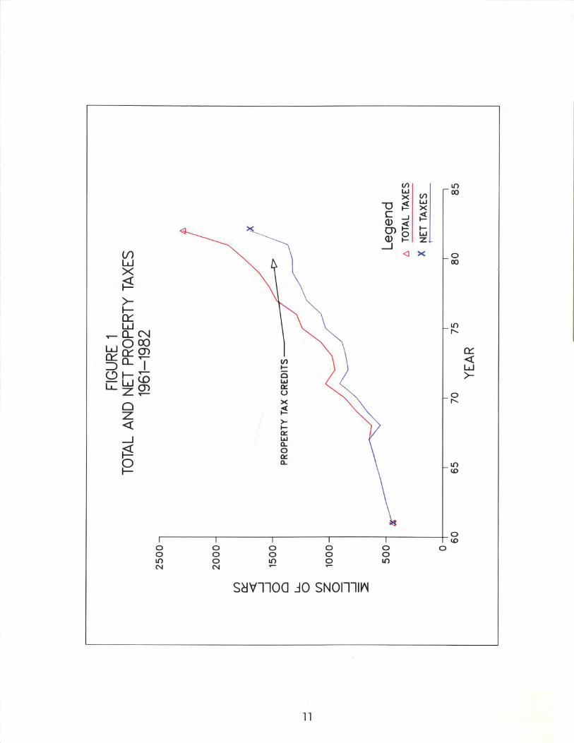
The reforms of 1967 resulted in only a one year reversal of the long standing trend of rising property taxes. Figure 1 presents data on total property taxes and property taxes after subtracting property tax credits, chiefly the homestead and agricultural credits.

As Figure 1 shows, between 1960 and 1967, property tax collections grew steadily at a rate that works out to be between 5.6 and 7.8 percent per year. There is no difference between the growth·· of total taxes and net property taxes since there were no state paid property tax credits during these years. Due to the Property Tax Relief Act of 1967, net property taxes declined 15.1 percent between 1967 and 1968, and total property taxes declined 3.1 percent. Net taxes decreased more than total taxes because of the homestead credit which became effective for taxes paid in 1968.

But following the decline between 1967 and 1968, taxes assumed an even faster rate of growth than before: 20.5 percent between 1968 and 1969; 14.4 percent between 1969 and 1970; and 19.3 percent between 1970 and 1971. Some analysts think the reason the property tax relief programs of 1967 did not provide long-lasting relief is that, in the absence of state mandated levy limits, local government and school districts reacted to the suddenly increased state aid as a windfall that could be spent with little impact on local taxpayers. I n addition, the late sixties were a time of high and increasing school enrollments and general population growth that put a great deal of financial pressure on schools and local government. By 1971, it was obvious that the property tax relief provided by the legislature in 1967 had been swallowed up by property tax increases during the next three years.

The Omnibus Tax Bill of 1971 incorporated a number of reforms that came to be called lithe Minnesota Miracle. 1I In part, the objective of this reform package was property tax relief, and as a consequence, between 1971 and 1972, the absolute level of the state­wide property tax levy shows an annual decline for only the second time in the preceding 40 years.

The main features of the 1971 package were:

• Increased school aid to be distributed in a new way de­signed to equalize tax effort necessary to fund a basic level of educational services;

• A new system of local government aids to counties, cities, and towns.

• A system of levy limitations for both school districts and units of local government designed to ensure that local spending would not increase as a result of increased state aid;

10

• State payment of the agricultural school mill rate differ­ential (now called the agricultural credit).

School districts and other local taxing districts were guar­anteed at least the level of aid received in 1970-71, so the potential of the 1971 reforms to equalize either tax effort or spending per pupil unit was limited. The impact on property taxes was clear, however; statewide, the effective property tax for education was reduced nearly 23 percent between 1971 and 1972. Total and net taxes both declined 8 percent between 1971 and 1972.

Following the reforms of the 1971 session, net taxes grew rather slowly (with the exception of 1975 and 1977) until 1982. This was accomplished by expanding direct and indirect property tax relief programs whenever it appeared that property taxes would go up too fast. Property taxes grew, for example, 2.3 percent between 1972 and 1973, 3.6 percent between 1975 and 1976, 0.2 percent between 1979 and 1980 and 2.8 percent between 1980 and 1981. But between 1981 and 1982 this trend changed; net taxes grew 24.3 percent, the first annual increase of this magnitude in history. This increase, which has been widely reported in the media, may create an impres­sion that once again Minnesota is faced with a "property tax problem." Indeed, any significant increase in taxes is a matter for concern. But for a more complete understanding of Minnesota's property tax situation, it is necessary to look beyond a one-year percentage in­crease. Therefore, in the next sections we examine what has hap­pened to property taxes over time:

• I n constant dollars;

• As a percent of market value;

• Per capita;

• Per $1,000 dollars of personal income; and

• On residential and agricultural property, the principal tar­gets of direct property tax relief programs.

We will find that tax levies on property as a whole have increased (in fact increased nearly every year since the state1s found­ing), but we will also find that other relevant factors have also changed--property values have escalated, incomes have grown, and government services have expanded. We will see that, even with the 1982 increase, property taxes over the last decade and a half have declined in relation to many other economic indicators.

c. THE PROPERTY TAX BURDEN IN MINNESOTA

1. PROPERTY TAXES IN CONSTANT DOLLARS

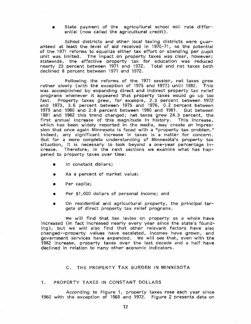
According to Figure 1, property taxes rose each year since 1960 with the exception of 1968 and 1972. Figure 2 presents data on

12

gross property taxes, taxes net of direct credits, and taxes net of direct credits and the circuit breaker. All figures are corrected for inflation using the national consumer price index (CP I) with 1967 as the base year. It is clear that net property taxes in constant dollars have not risen since 1971; they fell considerably even though they turned up sharply between 1981 and 1982. The major state property tax relief programs successfully kept property taxes from growing as fast as inflation. School aids and local government aids (indirect property tax relief programs) kept gross property taxes more or less constant in real dollars since 1972 and direct property tax relief programs, chiefly the agricultural and homestead credits, caused net taxes to decline about 24 percent between 1971 and 1982. In real dollars, property taxes are lower in 1982 than they were in 1965.

2. PROPERTY TAXES AS A PERCENT OF PERSONAL INCOME

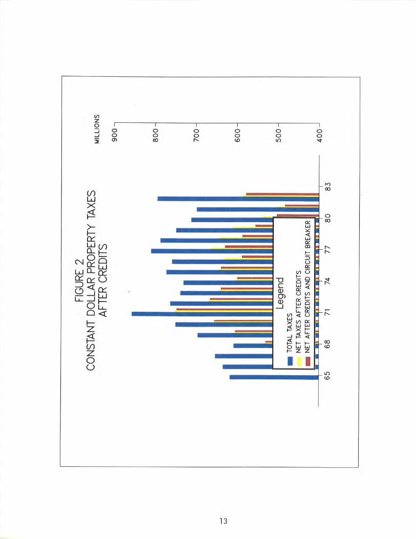
Another useful way to examine recent trends in the prop­erty tax is to look at the growth of property taxes in relation to changes in personal income in Minnesota and other states. Table 4 presents data from 1966 to 1981 on per capita personal income in Minnesota and Minnesota1s rank among other states, as well as prop­erty taxes and other broad based taxes per capita and per $1,000 of personal income. The statistics in Table 4, it should be noted, are based on all property taxes, not residential property taxes alone.

Minnesota1s per capita property tax rose from $165.28 in 1966 to $326.92 in 1981. But in relation to personal income, Minne­sota1s property tax declined considerably during this period, from $62.24 per $1,000 of personal income in 1966 to $33.53 in 1981. (These figures exclude property tax relief provided through the circuit breaker to homeowners and renters.) By this measure, Minne­sota1s property tax has declined more or less steadily since 1966. In 1966 Minnesota ranked 7th among the states in property tax per $1,000 of personal income. In 1981 it ranked 25th.

Minnesota1s income and sales tax collections per capita have increased over this period. Individual income taxes per $1,000 of personal income rose from $23.30 in 1966 to $35.14 in 1981. General sales taxes per $1,000 of personal income were $17.28 in 1981, up from 10.11 in 1968, the first year a general sales tax was levied in Minnesota.

A closer look at Table 4 shows the impact of major property tax reforms in 1967 and 1971. In 1967, prior to enactment of the reforms, Minnesota1s property tax per capita was $180.02, 5th highest among the states. By 1969, Minnesota ranked 22nd with a per capita tax of $156.02. But again, Minnesota1s relative position worsened and in 1972, per capita property taxes were $213.98, 12th highest in the nation. In 1973, when the reforms of the 1971 session took hold, Minnesota was 21 st among the states with a per capita property tax of $221.16.

I n summary, property taxes per capita and per $1,000 of personal income have declined markedly since 1966. When we look at residential and agricultural property taxes separately, it will become

14

TABL

E 4

MIN

NES

OTA

'S RA

NK F

OR S

ELEC

TED

TAXE

S FI

SCA

L YE

ARS

1967

-198

1

1966

19

67

1968

19

69

1970

19

71

1972

19

73

Am

ount

R

ank

Am

ount

R

ank

Am

ount

R

ank

Am

ount

R

ank

Am

ount

R

ank

Am

ount

R

ank

Am

ount

R

ank

Am

oU'ii

t R

ank

Per

Cap

ita

Per

sona

l In

com

e $

2,90

4 24

$

3,11

6 20

$

3,34

1 20

$

3,63

5 18

$

3,82

4 17

$

4,03

2 20

$

4,29

6 25

$

5,13

7 18

Sta

te a

nd

Loc

al

Tax

Rev

enue

s P

er C

apit

a $3

31. 7

5 9

$356

.99

7 $3

91. 7

0 7

$406

.15

11

$441

.96

15

$497

.70

12

$578

.00

8 $6

49.5

1 8

Per

$1,

000

of

Per

sona

l In

com

e 12

4.94

7

123.

27

5 12

7.94

5

123.

33

9 12

5.04

15

13

2.48

10

14

4.68

5

151.

15

4

Indi

vidu

al

Inco

me

Tax

Per

Cap

ita

$ 61

.88

7 $

69.2

2 7

$ 74

.77

6 $

82.2

0 9

$ 90

.86

10

$ 95

.52

9 $1

24.0

3 6

$150

.43

6 P

er $

1,00

0 o

f P

erso

nal

Inco

me

23.3

0 5

23.9

0 7

24.4

2 6

24.9

6 7

25.7

1 9

25.4

3 8

31.0

5 4

35.0

1 2

Pro

pert

y Ta

x P

er C

apit

a $1

65.2

8 7

$180

.02

5 $1

73.1

3 11

$1

56.0

2 22

$1

70.8

9 20

$2

10.6

7 13

$2

13.9

8 12

$2

21.1

6 21

P

er $

1,00

0 O

f P

erso

nal

Inco

me

62.2

4 7

62.1

6 6

56.5

5 9

47.3

7 21

48

.35

20

56.0

7 15

58

.07

13

51.4

7 19

Sal

es T

ax -

Gen

eral

P

er C

apit

a N

.A.

N.A

. $

31.0

1 40

$

47.0

2 34

$

51.4

1 37

$

54.8

1 41

$

69.3

3 37

$

76.8

1 38

P

er $

1,00

0 o

f P

erso

nal

Inco

me

N.A

. N

.A.

10.1

1 38

14

.28

35

14.5

5 37

14

.59

40

17.3

6 36

17

.87

37

--'

1974

19

75

1976

19

77

1978

19

79

1980

19

81

(J1

A

mou

nt

Ran

k A

mou

nt

Ran

k A

mou

nt

Ran

k A

mou

nt

Ran

k A

mou

nt

Ran

k A

mou

nt

Ran

k A

mou

nt

Ran

k A

mou

nt

Ran

k

Per

Cap

ita

Per

sona

l In

com

e $

5,44

2 19

$

5,80

7 22

$

6,18

3 25

$

7,12

9 18

$

7,91

0 19

$

8,86

5 19

$

9,72

4 18

$1

0,74

7'"

18

Sta

te a

nd

Loc

al

Tax

Rev

enue

s P

er C

apit

a $6

95.8

4 8

$754

.31

7 $8

22.6

8 7

$906

.10

9 $1

,001

.38

9 $1

,096

.29

8 $1

,124

.73

9 $1

,169

.63

11

Per

$1,

000

of

Per

sona

l In

com

e 13

6.15

8

139.

44

6 14

3.11

8

146.

92

7 14

1. 6

3 8

140.

40

7 12

7.41

9

119.

95

11

Indi

vidu

a·l

Inco

me

Tax

Per

Cap

ita

$179

.06

4 $2

05.5

8 3

$214

.25

4 $2

40.7

4 5

$268

.10

5 $3

09.3

6 3

$309

.71

6 $3

42.6

0 7

Per

$1,

000

of

Per

sona

l In

com

e 35

.04

2 38

.00

2 37

.27

2 39

.03

4 37

.92

4 39

.62

3 35

.08

7 35

.14

6

Pro

pert

y Ta

x P

er C

apit

a $2

16.9

0 22

$2

31.1

8 22

$2

54.2

0 24

$2

71.0

2 23

$3

00.8

5 23

$3

11.1

0 23

$3

24.1

9 22

$3

26.9

2 22

P

er $

1,00

0 o

f P

erso

nal

Inco

me

42.4

4 23

42

.73

23

44.2

2 22

43

.94

22

42.5

5 23

39

.84

22

36.7

2 22

33

.53

25

Sal

es T

ax -

Gen

eral

P

er C

apit

a $

88.8

8 37

$

97.9

1 35

$1

07.5

8 36

$1

17.6

9 38

$1

34.1

0 37

$1

49.7

5 35

$1

59.4

6 38

$1

68.4

7 36

P

er $

1,00

0 o

f P

erso

nal

Inco

me

17.3

9 37

18

.10

35

18.7

1 35

19

.04

36

18.9

7 37

19

.18

36

18.0

6 37

17

.28

36

N.A

. =

Not

App

lica

ble

(The

Gen

eral

S

ales

Tax

did

not

go

into

eff

ect

un

til

Fis

cal

Yea

r 19

68)

"'Fro

m U

.S.

Dep

artm

ent

of

Com

mer

ce,

Bur

eau

of

Econ

omic

Ana

lysi

s

Sou

rce:

U

.S.

Dep

artm

ent

of

Com

mer

ce,

Bur

eau

of

the

Cen

sus

Gov

ernm

enta

l F

inan

ce (

G.F

. N

o.3

and

5 b

y y

ear)

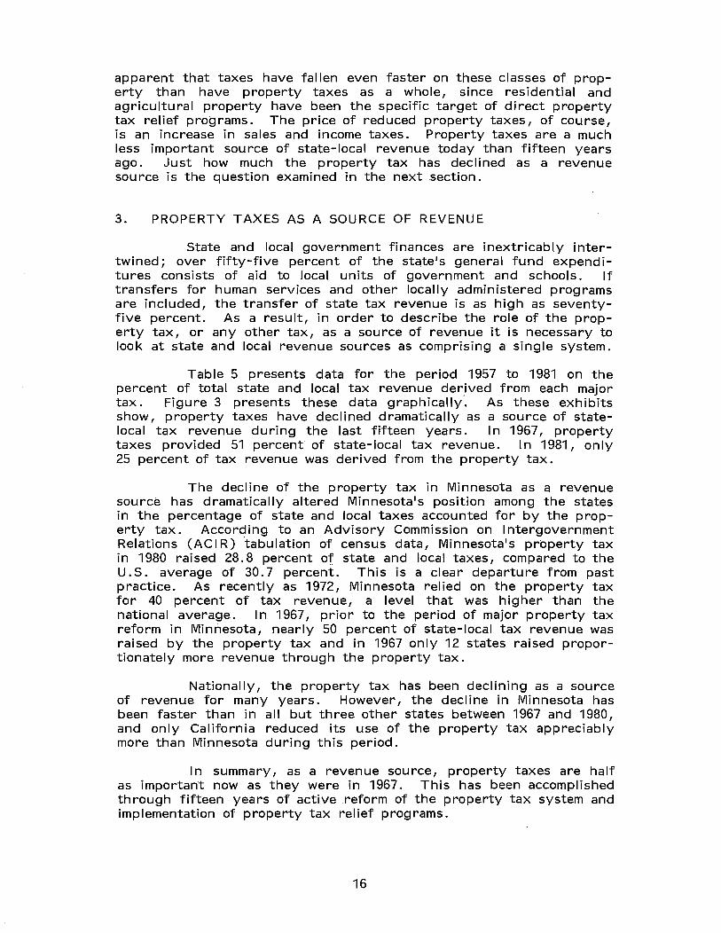
apparent that taxes have fallen even faster on these classes of prop­erty than have property taxes as a whole, since residential and agricultural property have been the specific target of direct property tax relief programs. The price of reduced property taxes, of course, is an increase in sales and income taxes. Property taxes are a much less important source of state-local revenue today than fifteen years ago. Just how much the property tax has declined as a revenue source is the question examined in the next section.

3. PROPERTY TAXES AS A SOURCE OF REVENUE

State and local government finances are inextricably inter­twined; over fifty-five percent of the state1s general fund expendi­tures consists of aid to local units of government and schools. If transfers for human services and other locally administered programs are included, the transfer of state tax revenue is as high as seventy­five percent. As a result, in order to describe the role of the prop­erty tax, or any other tax, as a source of revenue it is necessary to look at state and local revenue sources as comprising a single system.

Table 5 presents data for the period 1957 to 1981 on the percent of total state and local tax revenue derived from each major tax. Figure 3 presents these data graphically". As these exhibits show, property taxes have declined dramatically as a source of state­local tax revenue during the last fifteen years. In 1967, property taxes provided 51 percent of state-local tax revenue. In 1981, only 25 percent of tax revenue was derived from the property tax.

The decline of the property tax in Minnesota as a revenue source has dramatically altered Minnesota1s position among the states in the percentage of state and local taxes accounted for by the prop­erty tax. According to an Advisory Commission on Intergovernment Relations CACI R) 'tabulation of census data, Minnesota1s property tax in 1980 raised 28.8 percent of state and local taxes, compared to the U. S. average of 30.7 percent. This is a clear departure from past practice. As recently as 1972, Minnesota relied on the property tax for 40 percent of tax revenue, a level that was higher than the national average. In 1967, prior to the period of major property tax reform in Minnesota, nearly 50 percent of state-local tax revenue was raised by the property tax and in 1967 only 12 states raised propor­tionately more revenue through the property tax.

Nationally, the property tax has been declining as a source of revenue for many years. However, the decline in Minnesota has been faster than in all but three other states between 1967 and 1980, and only California reduced its use of the property tax appreciably more than Minnesota during this period.

I n summary, as a revenue source, property taxes are half as important now as they were in 1967. This has been accomplished through fifteen years of active reform of the property tax system and implementation of property tax relief programs.

16

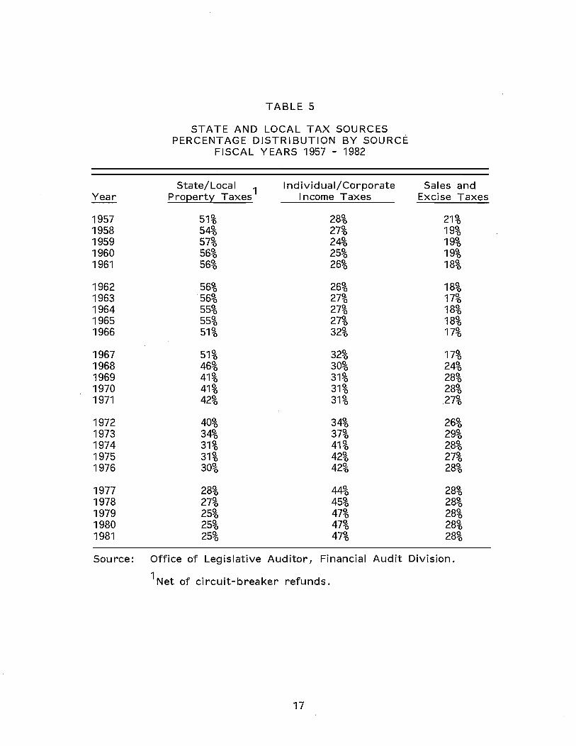
Year

1957 1958 1959 1960 1961

1962 1963 1964 1965 1966

1967 1968 1969 1970 1971

1972 1973 1974 1975 1976

1977 1978 1979 1980 1981

Source:

TABLE 5

STATE AND LOCAL TAX SOURCES PERCENTAGE DISTRIBUTION BY SOURCE

FISCAL YEARS 1957 - 1982

State/Local 1

Individual/Corporate Proeert~ Taxes I ncome Taxes

51% 28% 54% 27% 57% 24% 56% 25% 56% 26%

56% 26% 56% 27% 55% 27% 55% 27% 51% 32%

51% 32% 46% 30% 41% 31% 41% 31% 42% 31%

40% 34% 34% 37% 31% 41% 31% 42% 30% 42%

28% 44% 27% 45% 25% 47% 25% 47% 25% 47%

Office of Legislative Auditor, Financial Audit

1 Net of circuit-breaker refunds.

17

Sales and Excise Taxes

21% 19% 19% 19% 18%

18% 17% 18% 18% 17%

17% 24% 28% 28% 27%

26% 29% 28% 27% 28%

28% 28% 28% 28% 28%

Division.

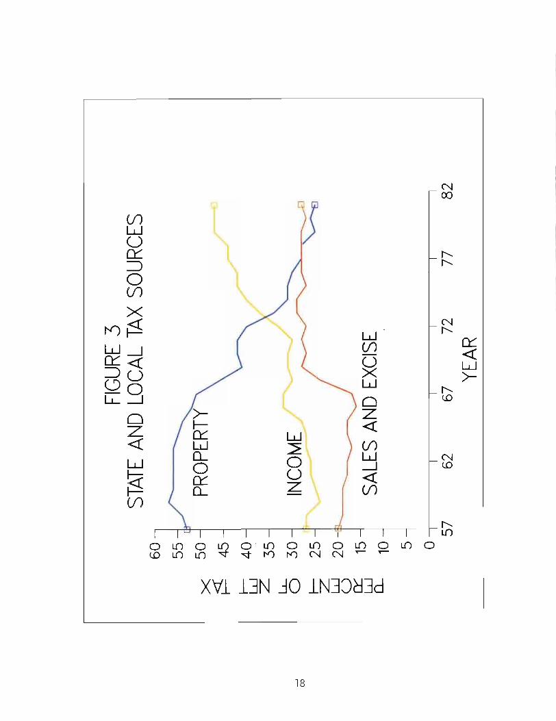
FIG

URE

3 ST

ATE

AND

LO

CAL

TAX

SO

UR

CES

60

55

X

50

~

45

r--40

w

Z

35

lL

.. 30

j IN

CO

ME../'

~

-'

0 co

25

"-...

---~

~

~

r-- z w

20 -

U

et::

15

SALE

S AN

D E

XCIS

E w

0.

... 10

5 0 ,

, ,

,

57

62

67

72

77

82

YEAR

4. EFFECTIVE PROPERTY TAX RATES

The effective tax rate (ETR) is the annual property tax (after credits) as a percent of market value. The effective tax rate can be computed for all property, specific classes of property, or for a single parcel. The ETR is commonly used and understood as a measure of property tax burden. As a measure of property tax levels, the effective tax rate is easily grasped. Proposition 13 in California and Proposition 2~ in Massachusetts limited residential prop­erty taxes as a percent of market value. I n Massachusetts property taxes were limited to an effective tax rate of two and one-half percent and in California to one percent.

This section examines what has happened to the effective tax rate in Minnesota over the last fifteen years and how Minnesota now compares to other states. In 1967, before the homestead credit and sales tax per capita aid, the effective tax rate for all real prop­erty was close to 3.0 percent. In 1968, the effective tax rate for all real property in Minnesota after subtracting the homestead credit was 2.3 percent. As we pointed out earlier, property taxes grew sharply between 1968 and 1971, 15-20 percent a year. As a result, the effective tax rate reached about 4.0 percept by 1971, a level many thought should not be allowed to go higher.

As a result of the property tax relief programs enacted in 1971 and subsequent years, and rapid inflation in real estate prices during the second half of the 1970s, the effective tax rate in Minne­sota has declined rapidly between 1975 and 1981. The effective tax rate on all classes of property was 2.42 percent in 1975, 1.80 percent in 1978, 1.16 percent in 1982. By 1982 it was about one-fourth of what it was in 1971 and about one-half of what it had been in 1977. These statistics which appear in Table 7 are discussed further in a later section. A declining tax as a percent of market value does not necessarily make it easier for people to pay their property taxes, although as we will see in the next section, the average property tax of Minnesota homeowners rose very little between 1975 and 1982 and actually declined in real dollars during this period.

5. AVERAGE PROPERTY TAX OF MINNESOTA HOMEOWNERS

Figures 4 and 5 present a data series that shows what has happened to average property taxes on Minnesota homes in current and constant dollars, between 1975 and 1982. As Figure 4 shows, average net property taxes increased between 1975 and 1982 from $465 to $511. As Figure 5 shows, in constant dollars, average taxes have declined during this period from $529 in 1975 to $314 in 1982. Aver­age property taxes in real dollars, however, turned upward in 1982 from a low of $280 in 1981.

1Effective tax rates for 1967 to 1971 are from Hatfield, Rolland F., Report to Governor1s Minnesota Property Tax Study Advisory Committee. November 1970.

19

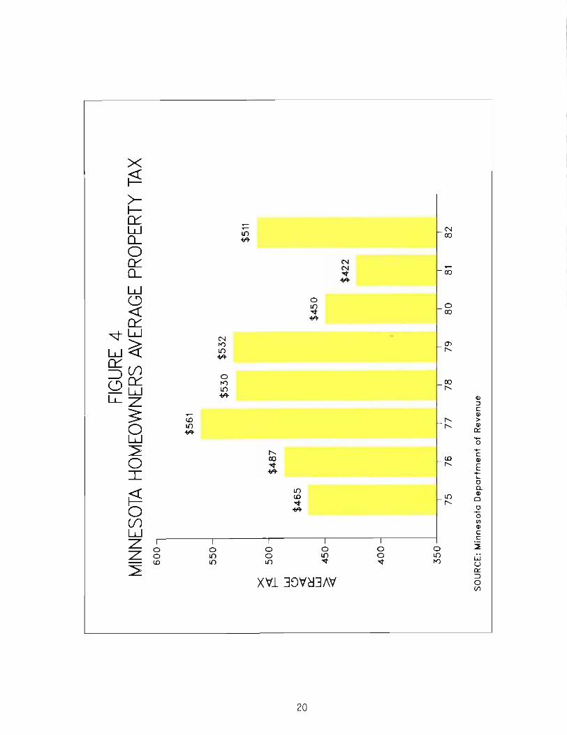
FIG

URE

4 M

INNE

SOTA

HO

MEO

WN

ERS

AVER

AGE

PRO

PER

TY T

AX

60

0- I

$561

55

0J

$5

30

$

53

2

$511

X ~

50

01

$4

87

w

$4

65

C

) N

«

C)

$4

50

~

w

45

0-

~

$4

22

I 400~

35

0

I I

I I

I I

I I

75

76

7

7

78

79

8

0

81

82

SO

UR

CE

: M

inn

eso

ta D

ep

art

me

nt

of

Re

ven

ue

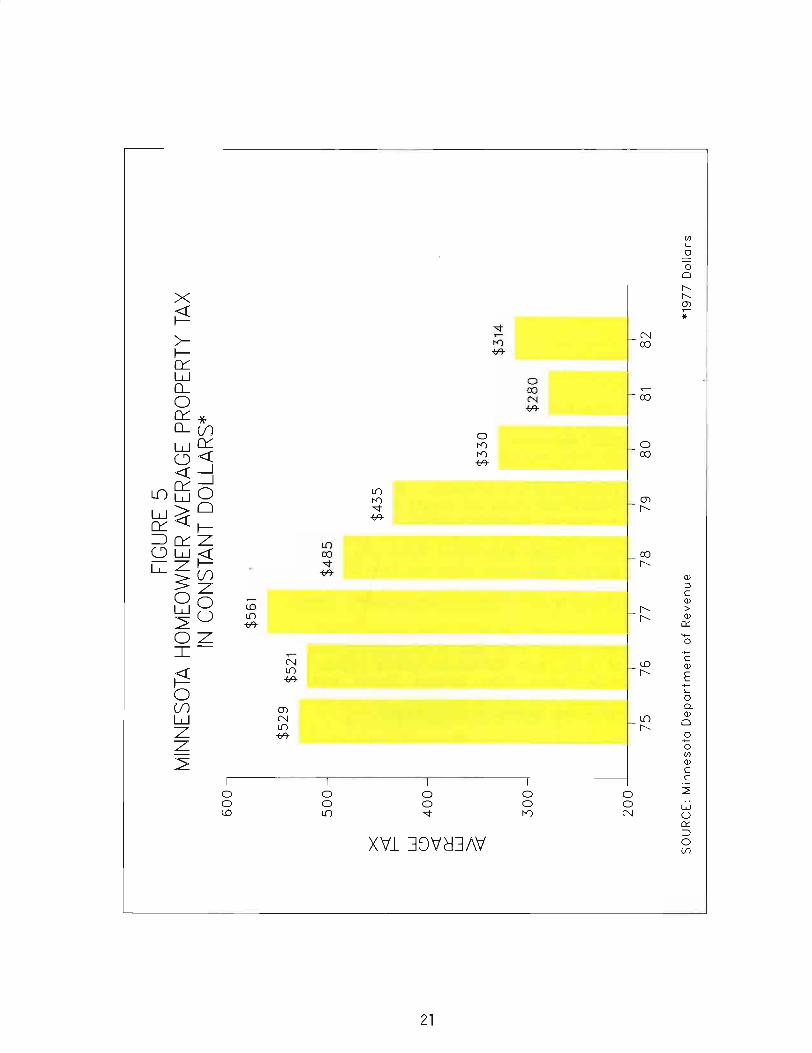
N

X ~

w

C) « 0:::

W ~

60

0 -

I

50

0-

40

0 -

300~

FIG

URE

5 M

INNE

SOTA

HO

MEO

WN

ER A

VERA

GE

PRO

PER

TY T

AX

IN C

ON

STA

NT

DO

LLA

RS*

$561

$5

29

$5

21

$4

85

$4

35

$3

30

$3

14

$2

80

20

0

I I

I I

I I

I I

I 7

5

76

7

7

78

7

9

80

81

8

2

SO

UR

CE

: M

inn

eso

ta D

ep

art

me

nt

of

Re

ven

ue

*1

97

7 D

olla

rs

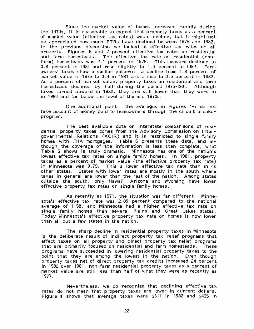
Since the market value of homes increased rapidly during the 1970s, it is reasonable to expect that property taxes as a percent of market value (effective tax rates) would decline, but it might not be appreciated how much ETRs have declined between 1975 and 1982. In the previous discussion we looked at effective tax rates on all property. Figures 6 and 7 present effective tax rates on residential and farm homesteads. The effective tax rate on residential (non­farm) homesteads was 2.1 percent in 1975. This measure declined to 0.8 percent in 1981 and rose slightly to 1.0 percent in 1982. Farm owners· taxes show a similar pattern: a decline from 1.3 percent of market value in 1975 to 0.4 in 1981 and a rise to 0.5 percent in 1982. As a percent of market value, property taxes on residential and farm homesteads declined by half during the period 1975-1981. Although taxes turned upward in 1982, they are still lower than they were in in 1980 and far below the level of the mid 1970s.

One additional point: the averages in Figures 4-7 do not take account of money paid to homeowners through the circuit breaker program.

The best available data on interstate comparisons of resi­dential property taxes comes from the Advisory Commission on I nter­governmental Relations (AC I R) and it is restricted to single family homes with FHA mortgages. Table 6 presents these data, and al­though the coverage of the information is less than complete, what Table 6 shows is truly dramatic. Minnesota has one of the nation·s lowest effective tax rates on single family homes. In 1981, property taxes as a percent of market value (the effective property tax rate) in Minnesota was 0.79. This a lower effective tax rate than in 42 other states. States with lower rates are mostly in the south where taxes in general are lower than the rest of the nation. Among states outside the south, only Hawaii, Arizona and Wyoming have lower effective property tax rates on single family homes.

As recently as 1971, the situation was far different. Minne­sota·s effective tax rate was 2.05 percent compared to the national average of 1.98, and Minnesota had a higher effective tax rate on single family homes than several Plains and Great Lakes states. Today Minnesota·s effective property tax rate on homes is now lower than all but a few states in the nation.

The sharp decline in residential property taxes in Minnesota is the deliberate result of indirect property tax relief programs that affect taxes on all property and direct property tax relief programs that are primarily focused on residential and farm homesteads. These programs have succeeded in lowering residential property taxes to the point that they are among the lowest in the nation. Even though property taxes net of direct property tax credits increased 24 percent in 1982 over 1981, non-farm residential property taxes as a percent of market value are still less than half of what they were as recently as 1977.

Nevertheless, we do recognize that declining effective tax rates do not mean that property taxes are lower in current dollars. Figure 4 shows that average taxes were $511 in 1982 and $465 in

22

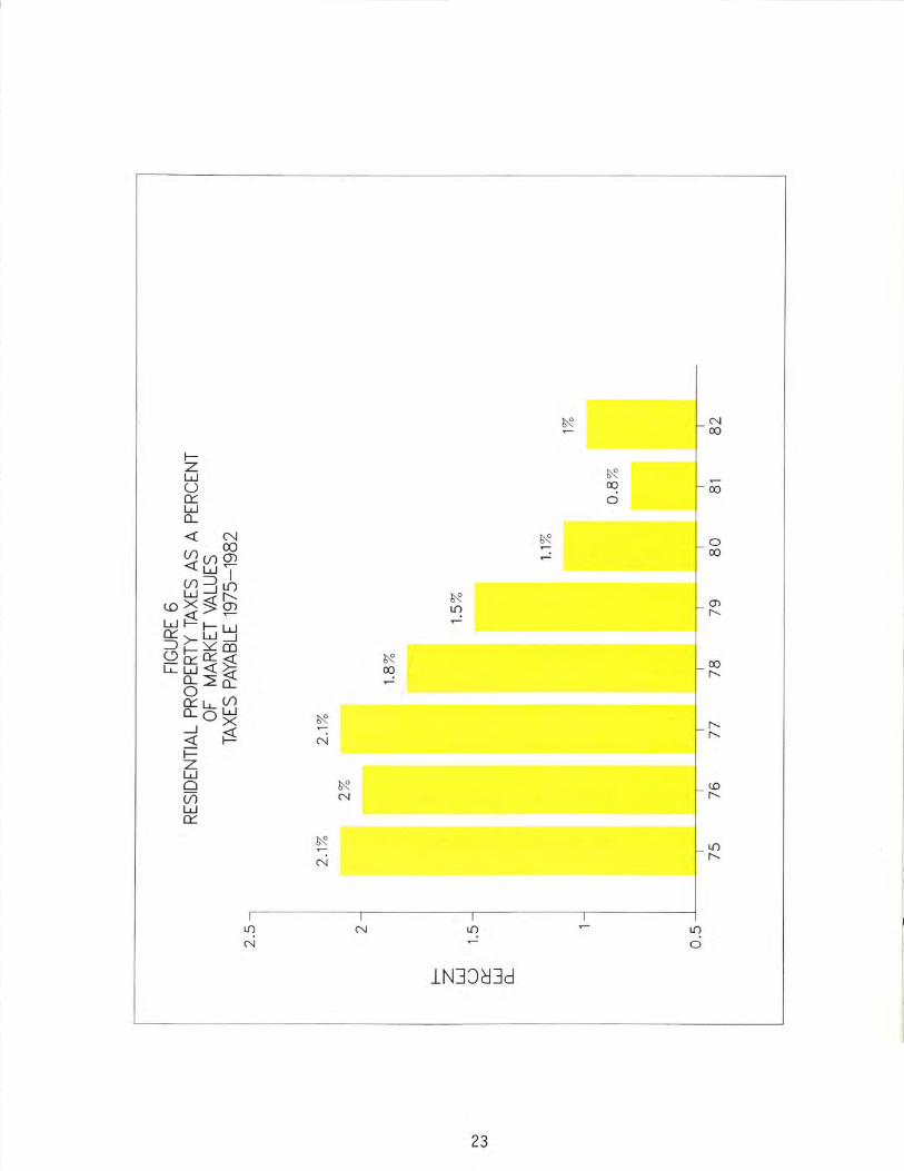
TABL

E 6

AVER

AGE

EFFE

CTIV

E PR

OPER

TY T

AX

RATE

S,

EXIS

TING

SIN

GLE

FAM

ILY

HOME

S W

ITH

1 FH

A IN

SURE

D M

ORTG

AGES

, BY

STA

TE A

ND

REGI

ON,

SELE

CTED

YEA

RS 1

95~ -

1981

Sta

te a

nd

Reg

ion

1981

19

80

1977

19

752

1971

19

66

1958

S

tate

and

R

egio

n 19

81

1980

19

77

1975

2 19

71

1966

19

58

--

--

UNIT

ED S

TATE

S 1.

26

1. 2

8 1.

67

1.89

1.

98

1. 7

0 1.

34

NEW

ENGL

AND

SOUT

HEAS

T

CONN

ECTI

CUT

1. 5

3 1.

55 3

2.17

1.

94

2.38

2.

01

1.44

AL

ABAM

A 0.

38

0.56

0.

74

0.75

0.

85

0.66

0.

56

MAI

NE

1.42

1.

25

1. 6

5 1.

86

2.43

2.

17

1. 5

8 AR

KANS

AS

1.42

1.

53

1.49

1.

41

1.14

1.

09

0.84

M

ASSA

CHUS

ETTS

2.

43

2.51

4 3.

50

3.26

3.

13

2.76

2.

21

FLOR

IDA

0.92

1.

02

1.13

1.

18

1.41

1.

09

0.76

NE

W HA

MPS

HIRE

N

.A.

1. 7

3 N

.A.

(2.3

8)

3.14

2.

38

1.81

GE

ORGI

A 1.

21

1. 2

4 1.

27

1. 3

3 1.

44

1. 3

0 0.

84

RHOD

E IS

LAND

N

.A.

1. 9

3 5 N

.A.

2.27

2.

21

1. 9

6 1.

67

KENT

UCKY

1.

14

1.19

1.

25

1. 2

3 1.

27

1. 0

3 0.

93

VERM

ONT

N.A

. 1.

60

N.A

. (2

.21)

2.

53

2.27

1.

63

LOUI

SIAN

A 0.

28

0.26

0.

61

0.64

0.

56

0.43

0.

52

MIS

SISS

IPPI

0.

86

0.93

1.

10

1.12

0.

96

0.93

0.

66

MID

EAST

NO

RTH

CARO

LINA

1.

07

0.95

1.

35

1. 5

1 1.

58

1.31

0.

90

SOUT

H CA

ROLI

NA

0.84

0.

81

0.82

1.

07

0.94

0.

60

0.48

DE

LAW

ARE

0.79

0.

85

0.88

0.

92

1.26

1.

14

0.71

TE

NNES

SEE

1. 4

2 1.

27

1.40

1.

31

1. 5

3 1.

37

0.97

D

IST.

OF

COL

UMBI

A 1.

22

1.30

n.

a.

1. 7

8 1.

80

1. 3

7 1.

08

VIR

GIN

IA

1. 3

9 1.

26

1.21

1.

32

1. 3

2 1.

13

0.90

MA

RYLA

ND

1. 2

5 1.

61

1.69

2.

01

2.24

2.

05

1.47

W

EST

VIR

GIN

IA

0.37

0.

43

N.A

. 0.

78

0.69

0.

71

0.56

NE

W JE

RSEY

2.

53

2.60

3.

31

3.15

3.

01

2.57

1.

77

NEW

YORK

2.

75

2.75

2.

89

2.56

2.

72

2.40

2.

09

SOUT

HWES

T PE

NNSY

LVAN

IA

1.50

1.

57

1.85

1.

71

2.16

1.

88

1. 5

0 AR

IZON

A 0.

74

1.16

1.

72

1. 5

4 1.

65

2.41

2.

14

GREA

T LA

KES

NEW

MEX

ICO

1.14

1.

12

1. 6

5 1.

56

1. 7

0 1.

30

0.93

OK

LAHO

MA

0.82

0.

91

0.95

1.

27

1. 3

5 1.

11

0.86

IL

LIN

OIS

1.

47

1. 5

0 1.

90

2.21

2.

15

1. 9

6 1.

35

TEXA

S 1.

68

1. 5

7 1.

84

2.06

1.

91

1.62

1.

36

INDI

ANA

1.13

1.

19

1. 66

1.

64

1. 9

6 1.

64

0.84

M

ICHI

GAN

2.74

2.

54

2.63

2.

38

2.02

1.

81

1.45

RO

CKY

MOU

NTAI

N N

OH

IO

1.07

1.

08

1. 2

6 1.

29

1.47

1.

44

1. 0

7 ~

WIS

CONS

IN

1. 7

5 1.

67

2.22

2.

63

3.01

2.

31

1.82

CO

LORA

DO

1. 0

1 1.

05

1.80

1.

99

2.45

2.

20

1.72

ID

AHO

0.94

0.

96

1.46

1.

86

1. 7

2 1.

23

1.14

PL

AINS

MO

NTAN

A 1.

08

1.11

1.

31

1. 6

0 2.

19

1. 7

0 1.

32

UTAH

1.

03

1. 0

2 1.

03

1. 2

0 1.

49

1. 5

2 1.

05

IOW

A 1.

75

1.48

1.

76

2.20

2.

63

2.12

1.

34

WYO

MING

0.

47

0.50

0.

87

1.12

1.

38

1. 3

4 1.

17

KANS

AS

0.93

0.

94

1. 3

7 1.

55

2.17

1.

96

1. 6

5 M

INNE

SOTA

0.

79

0.93

1.

39

1. 5

8 2.

05

2.14

1.

57

FAR

WES

T M

ISSO

URI

0.95

1.

00

1. 5

9 1.

85

1. 7

9 1.

64

1.12

NE

BRAS

KA

2.31

2.

37

2.48

2.

50

3.15

2.

67

1. 9

0 CA

LIFO

RNIA

1.

04

0.98

2.

21

2.08

2.

48

2.03

1.

50

NORT

H DA

KOTA

1.

01

1. 0

0 1.

26

1. 5

3 2.

08

1.81

1.

54

NEVA

DA

1.13

1.

22

1. 7

1 1.

53

1.48

1.

47

1.06

SO

UTH

DAKO

TA

1.69

1.

70

1. 7

9 2.

14

2.71

2.

64

2.01

OR

EGON

1.

56

1.72

2.

25

2.18

2.

33

1. 9

8 1.

55

WAS

HING

TON

0.95

1.

06

1. 7

5 1.

86

1. 6

2 1.

14

0.92

AL

ASKA

N

.A.

1. 3

5 N

.A.

1. 7

3 1.

61

1.42

1.

12

N.A

. --

DATA

NOT

AVA

ILAB

LE

HAW

AII

0.36

0.

42

N.A

. (0

.95)

0.

92

0.81

.0

.62

NOTE

: TH

ESE

EFFE

CTIV

E RA

TES

ARE

FOR

EXIS

TING

FH

A IN

SURE

D M

ORTG

AGES

ONL

Y,

WHI

CH

REPR

ESEN

T SM

ALL

AND

VARY

ING

PERC

ENTA

GES

(BY

STAT

E)

OF T

OTAL

SIN

GLE

-FA

MIL

Y HO

MES

. TH

ESE

RATE

S MA

Y OR

MAY

NO

T BE

REP

RESE

NTAT

IVE

OF T

HE

RATE

S AP

PLIC

ABLE

TO

ALL

HOME

S IN

A P

ARTI

CULA

R ST

ATE.

TH

E UN

ITED

STA

TES

AVER

AGE

TAX

RATE

FO

R 19

81 (

1.26

) IN

DICA

TES

THAT

, ON

AVE

RAGE

, TH

E PR

OPER

TY T

AX O

N A

HOM

E W

ITH

A M

ARKE

T VA

LUE

OF $

100,

000

WOU

LD

BE $

1,26

0.

~EFFECTIVE

TAX

RA

TE

IS T

HE

PERC

ENTA

GE T

HAT

TAX

LIA

BILI

TY

IS O

F TH

E M

ARKE

T OR

TRU

E VA

LUE

OF T

HE

HOUS

E.

FIGU

RES

IN

PARE

NTHE

SIS

ARE

FOR

1974

, DA

TA F

OR 1

975

NOT

AVAI

LABL

E.

3FOU

RTH

QUAR

TER

OF 1

977

INCR

EASE

D TO

198

0 ON

THE

BA

SIS

OF T

HE U

.S.

AVER

AGE

PERC

ENTA

GE C

HANG

E. 4A

CIR

STAF

F ES

TIM

ATES

BA

SED

ON 1

974

(LAT

EST

YEAR

RE

ADIL

Y AV

AILA

BLE)

IN

CREA

SED

TO 1

980

ON T

HE

BASI

S OF

THE

U.S

. AV

ERAG

E PE

RCEN

TAGE

CHA

NGE

(75%

) AN

D TH

E 19

77 C

ENSU

S OF

GOV

ERNM

ENTS

, "T

AXAB

LE

PROP

ERTY

VAL

UES

AND

ASSE

SSM

ENT/

SALE

S PR

ICE

RATI

OS"

(25%

). 5A

CIR

STAF

F ES

TIM

ATES

BA

SED

ON 1

974

(LAT

EST

YEAR

RE

ADIL

Y AV

AILA

BLE)

IN

CREA

SED

TO 1

980

ON T

HE B

ASI

S OF

THE

U

.S.

AVER

AGE

PERC

ENTA

GE C

HANG

E.

SOUR

CES:

CO

MPU

TED

BY A

CIR

STAF

F FR

OM D

ATA

CONT

AINE

D IN

U

.S.

DEPA

RTM

ENT

OF

HOUS

ING

AND

URBA

N DE

VELO

PMEN

T,

HOUS

ING

-FH

A,

MANA

GEME

NT

INFO

RMAT

ION

SYST

EMS

DIV

ISIO

N,

SING

LE-F

AMIL

Y IN

SURE

D BR

ANCH

, DA

TA F

OR S

TATE

S AN

D SE

LECT

ED A

REAS

ON

CHAR

ACTE

RIST

ICS

OF

FHA

OPER

ATIO

NS

UNDE

R SE

CTI

0ti

203b

),

VARI

OUS

YEAR

S.

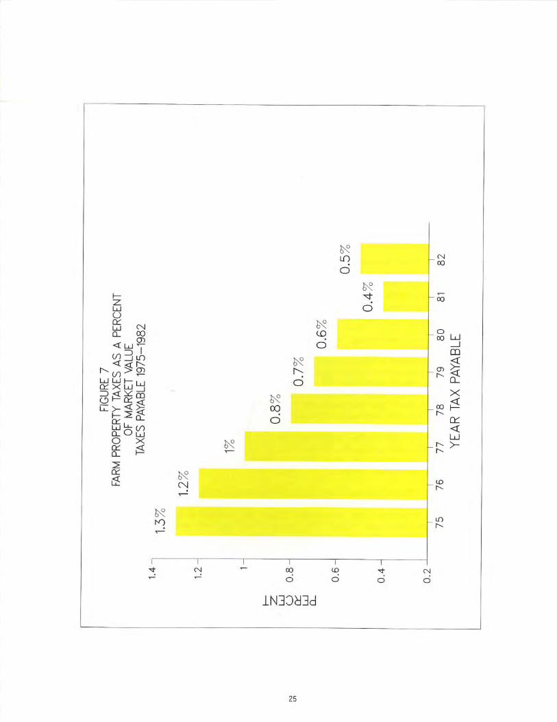
1975. Nor do increased housing values mean that low income home­owners have ready cash to pay property taxes.

Next we turn to an examination of what has happened to property taxes on other classes of property.

6. PROPERTY TAX RATES BY CLASS OF PROPERTY

I n Minnesota, as in about a quarter of the states in the union, different types of property are assessed at different fractions of market value for tax purposes. For example, in Minnesota the assessed value of unmined iron ore is set at 50 percent of market value, agricultural land not homesteaded at 19 percent of market value, the first $50,000 of agricultural homesteaded property at 14 percent of market value,' and the first $27,000 of other homesteads at 16 percent of market value.

The Minnesota classified property tax was authorized by a constitutional amendment in 1906 and first implemented by legislation in 1913. In recent years, the Legislature has frequently changed the classification system and, as a result, Minnesota now has the nation's most complicated classification system. There are more than fifty legal classes of property.

I n analyzing tax rates on classes of property, we com­pressed these legal classes into six use classes. This in also done by the Department of Revenue in computing assessment-sales ratios each year. Assessment-sales ratios are used by the Department of Revenue to adjust for variation in assessment practices across the state. Because school aids are distributed based on local tax effort, it is necessary for the department to study the relationship between assessed values and sales prices across the state in order to distrib­ute aid fairly. We used the department's sales ratios to compute accurate market value information for six use classes of property, then computed property taxes as a percent of market value (the effective tax rate) for each class before and after payment of direct property tax relief credits.

The effective tax rate is the best available way to compare tax levels across classes of property. Table 7 presents state-wide data on effective tax rates by class of property before and after direct property tax relief credits are applied for each year between 1975 and 1982. Also presented is the percentage by which ETRs have changed between 1975 and 1982 for taxes before and after state paid direct property tax relief Cfxcluding the income-adjusted property tax refund or circuit breaker).

10n a state-wide basis the circuit breaker for homeowners does not have much impact on the effective tax rate. In 1981, on residential property the ETR including the circuit breaker would be 0.71 percent instead of 0.83.

26

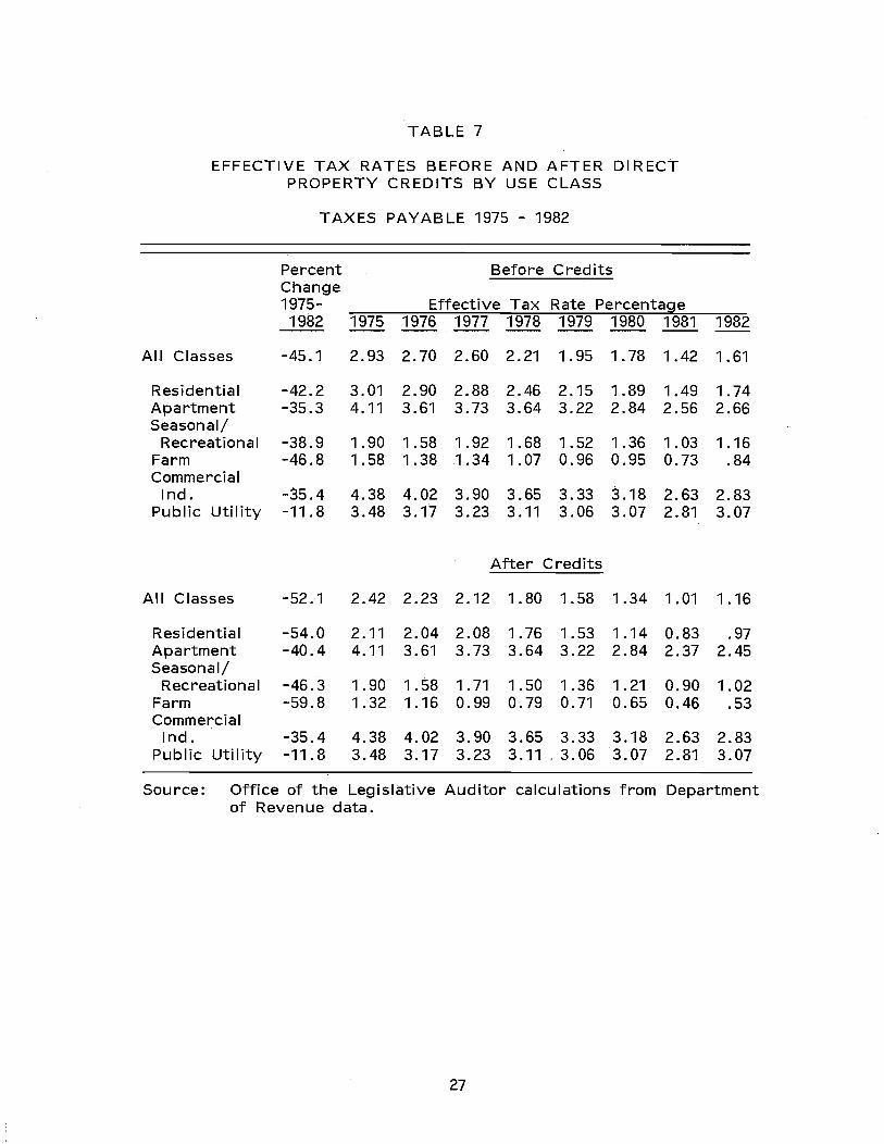
TABLE 7

EFFECTIVE TAX RATES BEFORE AND AFTER DIRECT PROPERTY CREDITS BY USE CLASS

TAXES PAYABLE 1975 - 1982

Percent Before Credits Change 1975- Effective Tax Rate Percenta~e

1982 1975 1976 1977 1978 1979 1980 1981 1982

All Classes -45.1 2.93 2.70 2.60 2.21 1.95 1.78 1.42 1.61

Residential -42.2 3.01 2.90 2.88 2.46 2.15 1.89 1.49 1.74 Apartment -35.3 4.11 3.61 3.73 3.64 3.22 2.84 2.56 2.66 Seasonal/

Recreational -38.9 1.90 1.58 1.92 1.68 1.52 1.36 1.03 1.16 Farm -46.8 1.58 1.38 1.34 1.07 0.96 0.95 0.73 .84 Commercial

Ind. -35.4 4.38 4.02 3.90 3.65 3.33 3.18 2.63 2.83 Public Utility -11.8 3.48 3.17 3.23 3.11 3.06 3.07 2.81 3.07

After Credits

All Classes -52.1 2.42 2.23 2.12 1.80 1.58 1.34 1.01 1.16

Residential -54.0 2.11 2.04 2.08 1.76 1.53 1.14 0.83 .97 Apartment -40.4 4.11 3.61 3.73 3.64 3.22 2.84 2.37 2.45 Seasonal/

Recreational -46.3 1.90 1.58 1.71 1.50 1.36 1.21 0.90 1.02 Farm -59.8 1.32 1.16 0.99 0.79 0.71 0.65 0.46 .53 Commercial

Ind. -35.4 4.38 4.02 3.90 3.65 3.33 3.18 2.63 2.83 Public Utility -11.8 3.48 3.17 3.23 3.11 . 3.06 3.07 2.81 3.07

Source: Office of the Legislative Auditor calculations from Department of Revenue data.

27

First, without state-paid direct property tax credits, prop­erty taxes have declined as a percent of market value on all classes of property. Growth in aid to schools and local government along with state financing of other local government obligations is respon­sible for part of this decline. Inflation in real property values also outran increases in the cost of providing government services and this caused a decline in the ETR. ETRs for residential, non­commercial seasonal recreational and farm property declined the most. Taxes on apartments, public utility property and commercial-industrial property declined less, although by a substantial amount.

Direct property tax credits lower effective tax rates on all classes except commercial-industrial and public utility property. The effective tax rate on residential property (after credits were applied) declined 54.0 percent between 1975 and 1982, and the ETR on farm property declined 59.8 percent during the same period. In 1982, the effective tax rate was 0.97 percent for residential property and 0.53 percent for farm property after direct property tax relief credits. Before direct tax credits, the ETR on residential and farm property was 1.74 and 0.84 percent respectively. Thus, direct property tax relief reduced the ETR 33 percent on residential property and 37 per­cent on farm property.

As we have noted before, the effective tax rate on residen­tial and farm property is low by historical standards in Minnesota and is also low compared to other states today. Effective tax rates are over twice as high on apartment property, commercial property and property owned by public utilities than on residential and farm prop­erty, because these classes are not generally eligible for direct prop­erty tax credits and their assessed value is set by law at a higher percentage of market value than are residential and farm property. However, effective tax rates on these classes of property have also declined since 1975 because of increases in indirect property tax relief.

D. CONCLUSION

Direct property tax relief programs are designed to keep property taxes low. Therefore, the first issue to be investigated in connection with a study of the relief programs is the question of whether. property taxes are high or low. Judging this question re­quires a look at changes in the property tax over time, comparison of Minnesota1s property tax to property taxes in other states, and an examination of property taxes in relation to other economic measures such as real estate values and personal income. We have made these comparisons and showed that Minnesota1s property taxes--residential property taxes in particular--are low in historical perspective and in comparison to other states. These low tax levels have been achieved through more than a decade of active reform of the property tax system and rapid expansion of property tax relief programs.

28

II. GEOGRAPHIC VARIATION IN .RESIDENTIAL PROPERTY TAXES

We have just reviewed historical trends in property taxes and the position of Minnesota relative to other states. On the whole, we have concluded that Minnesota's property taxes, especially resi­dential property taxes, are low in historical perspective and low compared to other states. I n the following section we look at varia­tion in property taxes across the state and discuss the significance of geographic variation for legislative decisions on direct property tax relief programs. The major points to be drawn from this section are:

• There is wide variation in the level of property taxes across Minnesota. While taxes are low, overall, as a result of 15 years of expanding property tax relief programs, taxes are especially low in some areas and relatively high in other areas. I n general, property taxes are highest in the Twin Cities metropolitan area and in other urban centers and relatively low in rural areas.

• Property taxes vary across communities for a number of reasons. Urban areas require relatively high taxes to finance services which are essential in such communities. High population density itself causes certain servi'tffis -to be either necessary or desirable.

• Taxes are also high in certain communities and not others because of a concentration of people needing public ser­vices, for example, children of school age or clients of public assistance programs.

• I n addition, taxes vary because of expenses induced by rapid growth, differences in property wealth and the prop­erty mix across communities, differing preferences for public services, and other factors.

• The wide variation in property taxes across the state helps to explain why, after years of little or no growth in prop­erty taxes, many people feel property taxes are too high. Because of the way it is structured, the homestead credit actually increases the difference in property taxes between high and low tax areas.

• Certain property tax relief programs are tied to variation in service needs or requirements across communities or the ability of individual taxpayers to pay property taxes. The homestead and agricultural credits, however, reduce taxes in a way that is riot tied directly to either service needs or ability to pay. Property tax relief programs such as these that work to reduce property taxes where they are already low (as well as where they are high) are hard to defend at a time of severe budget constraints and revenue shortfalls.

29

A. CAUSES OF GEOGRAPHIC VARIATION

The amount of tax paid on a particular parcel of property depends on its legal class, the budget and the property wealth of the taxing districts in which the parcel is located, and a parcells eligi­bility for property tax credits.

I n this section we examine in more detail why and by how much property taxes vary across the state. In addition, we examine how our system of property tax credits affects the geographic distri­bution of the property tax burden.

Figure 8 presents a simplified view of the factors affecting the amount of taxes paid on an individual parcel of property. Two types of factors are important: those associated with the taxing district as a whole and those specific to an individual parcel of prop­erty.

The first group of factors apply to all property in a taxing district and affect the mill rate. The mill rate in a taxing district is simply the taxing district's budget (after other sources of funds are subtracted) divided by the total amount of assessed value in the district. Mill rates vary because of several factors:

• Differences in service needs and requirements across com-munities. Different types of communities have different functional requirements.

• Differences in local preferences for public services.

• Differences in property wealth.

• Differences in the mix of property across taxing districts.

Functional requirements clearly differ between urban and rural communities. Urban or rapidly urbanizing communities require greater spending on public services and facilities than less developed or rural areas. While there are universal service needs and require­ments of urban centers, there are also optional amenities and pref­erences for public services that vary from one community to another.

Property wealth also varies and variation in wealth results in differing mill rates because lower wealth taxing districts must, in general, have higher mill rates to finance needed or preferred ser­vices.

Related to property wealth is the mix of legal property types in the taxing districts. Property mix affects the mill rate because of Minnesota's statutory property classification system. Each legal class of property is assessed for tax purposes at a specific rate. For example, commercial property is assessed at 43 percent of market value while residential homesteaded property is assessed at 16 percent on the first $27,000 in value, 22 percent on the next $27,000, and 28 percent on any market value above $54,000. As a result of

30

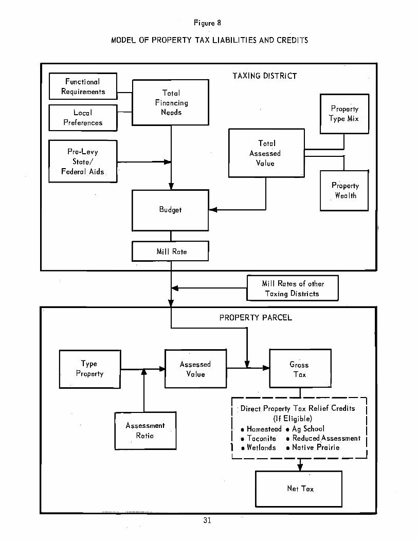
Figure 8

MODEL OF PROPERTY TAX LIABILITIES AND CREDITS

Functional TAXING DISTRICT

Requirements - Total Financing

Local I- Needs Property

Preferences Type Mix

I Total Pre~Levy Assessed

State/ Value I -Federal Aids

" Property

Wealth

Budget .. ~

i

Mill Rate

... Mill Rates of other .....

Taxing Districts

" PROPERTY PARCEL

Type Assessed ,r . Gross • Property ~~ Value Tax

r:-----1-----, I DirectProperty Tax Relief Credits I

Assessment I (If Eligible) I . • Homestead • Ag School I

Ratio I. Taconite • Reduced,Assessment I 1 • Wetlands • Native Prairie L ____ ~_--~---1

Net Tax

~.- -- ---- - .------

31

differences in classification, owners of some classes of property (for example, commercial) pay tax on a higher percentage of their property wealth. Thus, the mix of property affects the total assessed value in the district, and therefore the mill rate. For example, districts with a high percentage of market value in commercial property have a relatively higher total assessed value and, therefore, a relatively lower mill rate than districts with equal total market value but with a high percentage of residential property.

The second group of factors explaining property tax varia­tion is tied to the status of individual parcels of property. Once the mill rate for a taxing district is determined, the actual tax paid by property owners depends on the class and value of an individual parcel and whether or not the property is eligible for direct property tax relief programs. Eligibility for property tax credits is determined differently for each program. For residential homesteaded property, the market value is multiplied by the appropriate classification per­centages and the result is multiplied by the mill rate to give gross taxes. Homesteaded property is eligible for the homestead credit, so 58 percent of the gross tax up to $650 is subtracted from the gross tax to yield the net tax. On commercial property, the gross and net ,x is almost always the same since commercial property is generally

~ eligible for any direct credits.

The framework presented above can be used to understand wny property taxes vary across the state. The next section shows the actual net and gross tax variation across the state for residential property and examines this variation in more detail. However, no attempt is made precisely to attribute variation in taxes to any of the several causes of variation, such as service needs and requirements associated with particular kinds of communities, property mix, or local preferences. We show the extent of variation in taxes across the state relative to variation in property values and income because we believe this will help illuminate the political debate over property taxes and tax relief programs that is likely to occur in 1983, and because we believe that extensive geographic differences in property taxes are a problem that the legislature may wish to address, espe­cially because the homestead credit reduces property taxes less in high tax areas than low tax areas and thus increases rather than diminishes geographic differences.

B. RESIDENTIAL PROPERTY TAXES

The remainder of this chapter examines, in turn, geograph­ic variation in taxes on residential (non-farm) and farm homesteads. These receive nearly all the property tax relief provided through direct property tax relief programs. Estimates of the total state paid direct property tax credits on residential homesteads totalled $437,265,000 in 1982, and $125,357,000 for farm homesteads.

Table 8 shows the average net property tax on non-farm homesteads by county for 1982. Average property taxes vary greatly across the state. The highest average tax was $911 in Hennepin

32

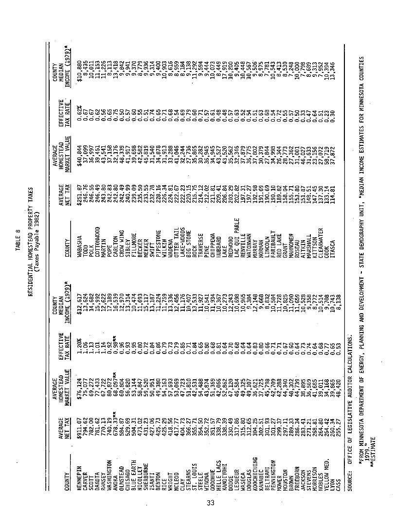
TABL

E 8

RESI

DENT

IAL

HOM

ESTE

AD P

ROPE

RTY

TAXE

S (T

axes

Pa

yabl

e 19

82)

AVER

AGE

COUN

TY

AVER

AGE

COUN

TY

AVER

AGE

HOM

ESTE

AD

EFFE

CTIV

E HE

DIAN

AV

ERAG

E Ho

t1EST

EAD

EFFE

CTIV

E M

EDIA

N CO

UNTY

NE

T TA

X M

ARKE

T VA

LUE

TAX

RA

IL

INCO

ME

~1979l*

COUN

TY

NET

TAX

MAR

KET

VALU

E TA

X R

ATE

' IN

Cot,lE

{19

79)*

HENN

EPIN

$9

11.0

7 $7

6,12

4 1.

20%

$1

2,61

7 W

ABAS

HA

$251

.87

$40,

844

0.62

%

$10,

880

CARV

ER

794.

62

75,0

77

1.06

13

,624

TO

DD

246.

76

37,0

99

0.67

8,

435

SCOT

T 78

2.00

69

,272

1.

13

14,6

82

POLK

24

6.55

36

,997

0.

67

10,0

11

DAKO

TA

781.

62

77,4

33

1.01

15

,992

CO

TTON

I-/OOD

24

6.49

39

,451

0.

62

11,1

53

RAI4S

EY

770.

13

67,7

22

1.14

12

,622

I1A

RTIN

24

3.80

43

,541

0.

56

11,2

26

WAS

HING

TON

740.

19

80,8

72

0,92

17

,189

PO

PE

242.

83

37,1

58

0.65

8,

113

ANOK

A 67

8.33

**

68,0

97**

0.

98**

16

,539

CA

RLTO

N 24

2.80

32

,176

0.

75

13,4

18

OLNS

TEAD

58

4.87

60

,804

0.

96

12,9

70

CROW

WIN

G 24

2.49

48

,339

0.

50

9,84

2 CH

ISAG

O 52

9.69

56

,820

0.

93

13,3

14

SIBL

EY

240.

99

41,9

17

0.57

9,

941

BLUE

EA

RTH

504.

31

53,1

44

0.95

10

,474

FI

LLM

ORE.

23

9.09

39

,698

·0

.60

9,37

0 NI

COLL

ET

473.

02

58,8

47

0.80

11

,693

BE

CKER

23

5.50

42

,582

0.

55

8,77

9 SH

ERBU

RNE

431.

23

59,5

20

0.72

15

,117

M

EEKE

R 23

3.55

45

,819

0.

51

9,93

6 IS

AN

TI

427.

06

50,9

51

0.84

13

,187

SW

IFT

232.

78

31,5

40

0.74

9,

314

BENT

ON

425.

73

49,3

80

0.86

11

,224

PI

PEST

ONE

228.

16

34,8

78

0.65

9,

400

RICE

42

5.29

54

,163

0.

79

11,7

59

WIL

KIN

226.

34

31,9

13

0.71

10

,903

W

RIGH

T 41

8.56

57

,693

0.

73

13,3

36

\oIAD

ENA

224.

81

33,2

88

0.68

8,

616

MCLE

OD

417.

77

53,0

69

0.79

12

,456

OT

TER

TAIL

22

2.67

41

,046

0.

54

8,95

9 CL

AY

404.

73

47,7

23

0.85

11

,176

LA

KE-\'1

00DS

22

2.23

32

,244

0.

69

8,18

4 ST

EARN

S 36

6,27

51

,810

0.

71

10,4

07

BIG

STON

E 22

0.15

27

,736

0.

79

9,13

8 ST

. LO

UIS

355.

71

42,5

31

0.84

13

,533

RO

CK

215.

75

35,8

65

0.60

.

11,2

92

STEE

LE

354.

50

54,4

88

0.65

11

,927

TR

AVER

SE

214.

12

30,2

82

0.71

9,

594

w

WIN

ONA

352.

72

43,8

74

0.80

10

,541

PI

NE

212.

02

36,9

45

0.57

9,

444

w

GOOD

HUE

351.

57

51,3

69

0.68

11

,934

CH

IPPE

WA

211.

81

34,9

45

0.61

10

,073

m

LLE

LACS

33

8.79

42

,066

0.

81

10,3

67

HUBB

ARD

209.

41

43,5

27

0.48

8,

449

KAND

IYOH

I 33

8.39

52

,862

0.

64

10,2

73

LAKE

20

6.84

43

,520

0.

48

17,9

19

DODG

E 33

0.49

47

,120

0.

70

12,2

43

REDI

'100D

20

3.29

35

,562

0.

57

.10,

?00

LESU

EUR

317.

86

46,5

84

0.68

10

,698

LA

C QU

I PA

RLE

202.

82

32,3

46

0.63

9,

405

WAS

ECA

315.

80

49,3

25

0,64

10

,965

RE

NVIL

LE

197.

31

37,8

79

0.52

10

.,448

DO

UGLA

S 31

2.65

49

,107

0.

64

9,38

4 WA

TONW

AN

197.

27

36,7

75

0.54

10

,567

KO

OCHI

CHIN

G 30

4.25

36

,621

0.

83

12,1

48

MURR

AY

192.

98

37,8

02

0.51

9,

506·

KA

NABE

C 30

2.51

37

,725

0.

80

9,66

8 NO

Rr1A

N 19

1. 6

9 30

,379

0.

63

8,97

5 BE

LTRA

1·1I

301.

93

45,7

98

0.66

8,

832

LINC

OLN

190.

69

27,8

44

0.68

7,

781

PENN

INGT

ON

301.

27

42,7

09

0.71

10

,584

FA

RIBA

ULT

190.

10

34,9

98

0.54

10

,543

14

0HER

29

9.37

42

,288

0.

71

11,7

28

RED

LAKE

18

9.82

26

,344

0.

72

8,41

3 HO

USTO

N 29

7.11

44

,340

0.

67

10,8

25

GRAN

T 15

8.04

28

,773

0.

55

8,53

0 BR

OWN

289.

33

48,3

02

0.60

11

,090

MA

HNOM

EN

155.

71

27,3

62

0.57

7,

248

FREE

BORN

28

6.34

44

,739

· 0.

64

11,6

59

ROSE

AU

153.

80

31,0

01

0.50

10

,000

JA

CKSO

N 28

3.41

38

,895

0.

73

10,5

28

AITK

IN

151.

87

46,0

27

0.33

7,

798

STEV

ENS

271.

21

36,5

69

0.74

9,

358

MAR

SHAL

L 14

8.51

31

,633

0.

47

8,68

9 Ho

RRIS

ON

268.

81

41,6

85

0.64

8,

772

KIIT

SON

147.

45

23,1

56

0.64

9,

313

NOBL

ES

264.

80

39,0

11

0.68

10

,514

CL

EARW

ATER

13

7.30

27

,072

0.

51

7,95

2 YE

LLOW

MEO

. 26

4.42

34

,168

0.

77

9,70

8 CO

OK

133.

14

58,7

19

0.23

10

,394

LY

ON

260.

34

39,8

65

0.65

10

,743

IT

ASCA

11

4.81

37

,872

0.

30

13,3

46

CASS

25

5.27

48

,420

0.

53

8,13

8

SOUR

CE:

OFFI

CE O

F LE

GISL

ATIV

E AU

DITO

R CA

LCUL

ATIO

NS.

*FRo

M M

INNE

SOTA

DEP

ARTM

ENT

OF E

NERG

Y,

PLAN

NING

AND

DEV

ELOP

MEN

T -

STAT

E DE

MOG

RAPH

Y U

NIT

, IIM

EDIA

N IN

COM

E ES

TIM

ATES

FOR

MIN

NESO

TA C

OUNT

IES

1979

.11

**ES

TIM

ATE

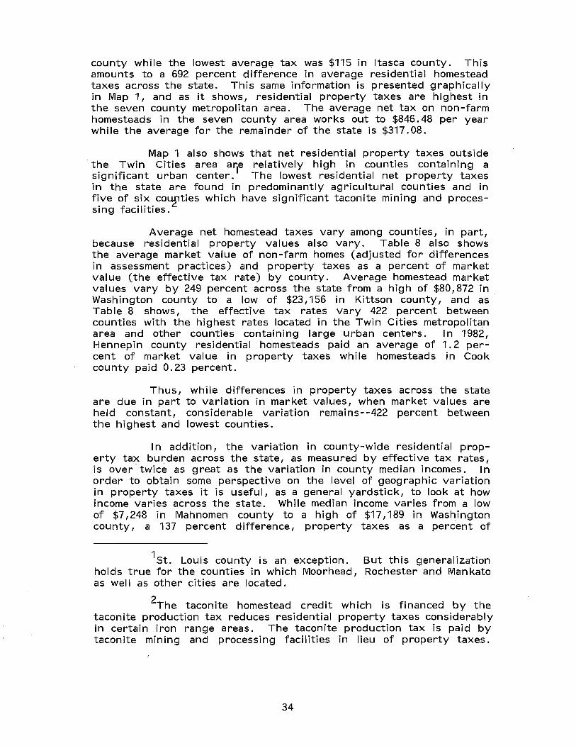
county while the lowest average tax was $115 in Itasca county. This amounts to a 692 percent difference in average residential homestead taxes across the state. This same information is presented graphically in Map 1, and as it shows, residential property taxes are highest in the seven county metropolitan area. The average net tax on non-farm homesteads in the seven county area works out to $846.48 per year while the average for the remainder of the state is $317.08.

Map 1 also shows that net residential property taxes outside the Twin Cities area a~e relatively high in counties containing a significant urban center. The lowest residential net property taxes in the state are found in predominantly agricultural counties and in five of six cOLPties which have significant taconite mining and proces­sing facilities.

Average net homestead taxes vary among counties, in part, because residential property values also vary. Table 8 also shows the average market value of non-farm homes (adjusted for differences in assessment practices) and property taxes as a percent of market value (the effective tax rate) by county. Average homestead market values vary by 249 percent across the state from a high of $80,872 in Washington county to a low of $23,156 in Kittson county, and as Table 8 shows, the effective tax rates vary 422 percent between counties with the highest rates located in the Twin Cities metropolitan area and other counties containing large urban centers. In 1982, Hennepin county residential homesteads paid an average of 1.2 per­cent of market value in property taxes while homesteads in Cook county paid 0.23 percent.

Thus, while differences in property taxes across the state are due in part to variation in market values, when market values are held constant, considerable variation remains--422 percent between the highest and lowest counties.

I n addition, the variation in county-wide residential prop­erty tax burden across the state, as measured by effective tax rates, is over' twice as great as the variation in county median incomes. In order to obtain some perspective on the level of geographic variation in property taxes it is useful, as a general yardstick, to look at how income varies across the state. While median income varies from a low of $7,248 in Mahnomen county to a high of $17,189 in Washington county, a 137 percent difference, property taxes as a percent of

1 St. Louis county is an exception. But this generalization holds true for the counties in which Moorhead, Rochester and Mankato as well as other cities are located.

2The taconite homestead credit which is financed by the taconite production tax reduces residential property taxes considerably in certain iron range areas. The taconite production tax is paid by taconite mining and processing facilities in lieu of property taxes.

34

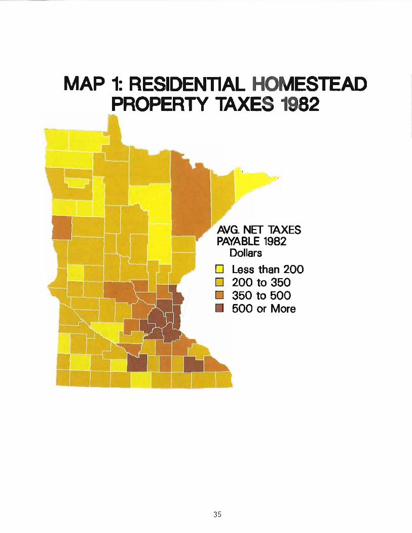
I I

I

MAP 1: RESIDENTIAL HOMESTEAD PROPERTY TAXES 1982

I '

AVG. NET TAXES PAYABLE 1982

Dollars

D Less than 200 D 200 to 350 D 350 to 500 • 500 or More

35

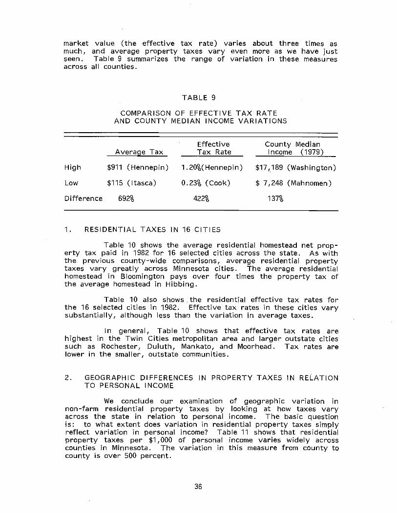
market value (the effective tax rate) varies about three times as much, and average property taxes vary even more as we have just seen. Table 9 summarizes the range of variation in these measures across all counties.

High

Low

Difference

TABLE 9

COMPARISON OF EFFECTIVE TAX RATE AND COUNTY MEDIAN INCOME VARIATIONS

Effective County Median Average Tax Tax Rate Income (1979)

$911 (Hennepin) 1.20%(Hennepin) $17,.189 (Washington)

$115 ( Itasca) 0.23% (Cook) $ 7,248 (Mahnomen)

692% 422% 137%

1. RESIDENTIAL TAXES IN 16 CITIES

Table 10 shows the average residential homestead net prop­erty tax paid in 1982 for 16 selected cities across the state. As with the previous county-wide comparisons, average residential property taxes vary greatly across Minnesota cities. The average residential homestead in Bloomington pays over four times the property tax of the average homestead in Hibbing.

Table 10 also shows the residential effective tax rates for the 16 selected cities in 1982. Effective tax rates in these cities vary substantially, although less than the variation in average taxes.

In general, Table 10 shows that effective tax rates are highest in the Twin Cities metropolitan area and larger outstate cities such as Rochester, Duluth, Mankato, and Moorhead. Tax rates are lower in the smaller, outstate communities.

2. GEOGRAPHIC DIFFERENCES IN PROPERTY TAXES IN RELATION TO PERSONAL INCOME

We conclude our examination of geographic variation in non-farm residential property taxes by looking at how taxes vary across the state in relation to personal income. The basic question is: to what extent does variation in residential property taxes simply reflect variation in personal income? Table 11 shows that residential property taxes per $1,000 of personal income varies widely across counties in Minnesota. The variation in this measure from county to county is over 500 percent.

36

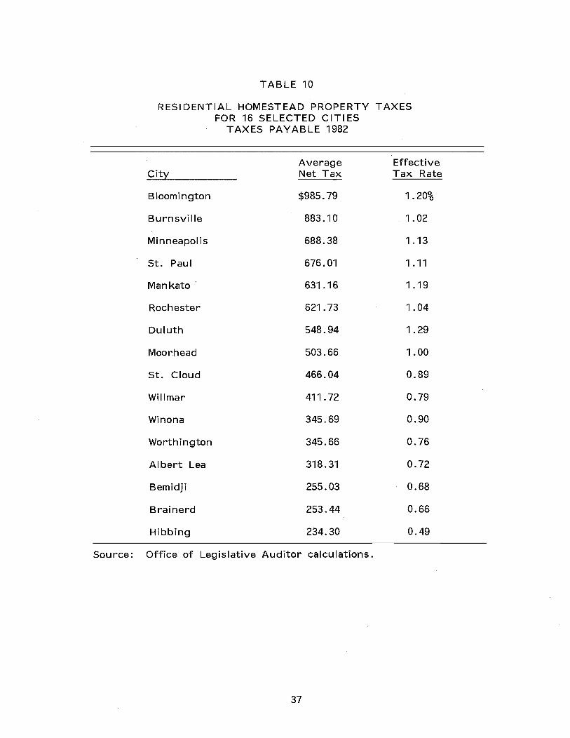
TABLE 10

RESIDENTIAL HOMESTEAD PROPERTY TAXES FOR 16 SELECTED CITIES

TAXES PAYABLE 1982

Average Effective City Net Tax Tax Rate

Bloomington $985.79 1.20%

Burnsville 883.10 1.02

Minneapolis 688.38 1.13

St. Paul 676.01 1.11

Mankato 631.16 1.19

Rochester 621.73 1.04

Duluth 548.94 1.29

Moorhead 503.66 1.00

St. Cloud 466.04 0.89

Willmar 411.72 0.79

Winona 345.69 0.90

Worthington 345.66 0.76

Albert Lea 318.31 0.72

Bemidji 255.03 0.68

Brainerd 253.44 0.66

Hibbing 234.30 0.49

Source: Office of Legislative Auditor calculations.

37

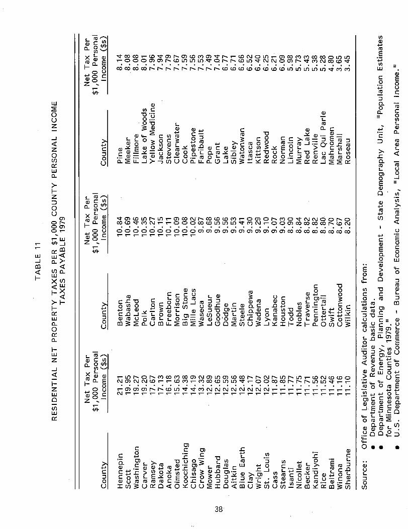
w

00

TA

BL

E 1

1

RE

SID

EN

TIA

L

NE

T

PR

OP

ER

TY

TA

XE

S

PER

$

1,0

00

C

OU

NT

Y

PE

RS

ON

AL

IN

CO

ME

T

AX

ES

P

AyA

BL

E 1

979

Net

Tax

P

er

Net

Tax

P

er

Net

Tax

P

er

$1

,00

0

Per

son

al

$1

,00

0

Per

son

al

$1

,00

0

Per

son

al

Co

un

ty

Inco

me

($s)

C

ou

nty

In

com

e ($

s)

Co

un

ty

Inco

me

($s)

Hen

nep

in

21.2

1 B

ento

n

10

.84

P

ine

8.1

4

Sco

tt

19

.95

W

abas

ha

10

.69

M

eek

er

8.0

8

Was

hin

gto

n

19

.27

M

cLeo

d 1

0.4

6

Fil

lmor

e 8

.08

C

arv

er

19

.20

P

olk

1

0.3

5

Lak

e o

f W

oods

8

.01

R

amse

y

17

.67

C

arlt

on

1

0.2

7

Yel

low

M

edic

ine

7.9

6

Dak

ota

1

7.1

3

Bro

wn

1

0.1

5

Jack

son

7

.94

A

no

ka

16

.18

F

reeb

orn

1

0.1

1

Ste

ven

s 7

.79

O

lmst

ed

15

.63

M

orr

iso

n

10

.09

C

lear

wat

er

7.6

7

Koo

ch ic

h i n

g

14

.38

B

ig S

ton

e 1

0.0

8

Co

ok

7

.59

C

his

ago

1

4.1

9

Mil

le

Lac

s 1

0.0

2

Pip

esto

ne

7.5

6

Cro

w W

ing

13

.32

W

asec

a 9

.87

F

arib

ault

7

.53

M

ower

1

2.8

9

LeS

ueu

r 9

.68

P

op

e 7.

.49

Hu

bb

ard

1

2.6

5

Go

od

hu

e 9

.56

G

ran

t 7

.. 04

Do

ug

las

12

.59

D

od

ge

9.5

6

Lak

e 6

.77

A

itk

in

12

.56

M

arti

n

9.5

3

Sib

ley

6.

71

Blu

e E

arth

1

2.4

8

Ste

ele

9.4

1

Wat

onw

an

6.6

6

Cla

y

12

.17

C

hip

pew

a 9

.30

It

asca

6

.52

W

rig

ht

12

.07

W

aden

a 9

.29

K

itts

on

6

.40

S

t.

Lou

is

12

.02

L

yon

9.1

0

Red

woo

d 6

.25

C

ass

11

.87

K

anab

ec

9.0

7

Roc

k 6

.21

· S

tearn

s 1

1.8

5

Ho

ust

on

9

.03

N

orm

an

6.0

9

Isan

ti

11

.77

T

od

d

8.9

0

Lin

coln

5

.98

N

icol

let

11

.75

N

oble

s 8

.84

M

urr

ay

5.7

3

Bec

ker

1

1.7

1

Tra

vers

e

8.8

2

Red

L

ake

5.4

3

Kan

diy

oh

i 1

1.5

6

Pen

nin

gto

n

8.8

2

Ren

vil

le

5.3

8

Ric

e 1

1.5

2

Ott

erta

il

8.8

0

Lac

Qui

P

arle

5

.28

B

eltr

ami

11

.46

S

wif

t 8

.70

M

ahno

men

4

.80

W

inon

a 1

1.1

6

Co

tto

nw

oo

d

8.6

7

Mar

shal

l 3

.65

S

herb

urn

e

11

.10

W

ilki

n 8

.20

R

ose

au

3.4

5

So

urc

e:

Off

ice

of

Leg

isla

tiv

e A

ud

ito

r ca

lcu

lati

on

s fr

om

: •

Dep

artm

ent

of

Rev

enu

e b

asic

data

. •

Dep

artm

ent

of

En

erg

y,

Pla

nn

ing

an

d

Dev

elo

pm

ent

-S

tate

D

emo

gra

ph

y

Un

it,

IIP

opul

atio

n E

stim

ates

fo

r M

inn

eso

ta

Co

un

ties

197

9. II

• U

.S.

Dep

artm

ent

of

Com

mer

ce -

Bu

reau

of

Eco

nom

ic A

nal

ysi

s,

II L

ocal

A

rea

Per

son

al

Inco

me.

II

Map 2 is a graphic presentation of the data shown in Table 11. Residential taxes per $1,000 personal income are shown to be highest in the seven county metropolitan area. Tax burdens in this part of the state vary from $16.18 in Anoka county to $21.21 in Hennepin county. Taxes are lowest according to this measure in outstate agricultural counties with Roseau county showing the lowest burden of $3.45.

A comparison of variation in taxes per $1,000 personal income to the previously discussed measures of tax burden shows that the geographic distribution of all measures is remarkably similar. Counties in the Twin Cities area and counties with large population centers have a relatively high property tax burden while - rural, predominately agricultural counties have lower taxes. Certain north­ern counties without high agricultural property wealth such as Becker, Hubbard, Cass and Aitkin show a high tax burden using the tax per $1,000 income measure, while their residential effective tax rates are low.

In summary, residential property tax burdens vary dramati­cally across the state. The magnitude in variation for all measures is well over 400 percent, suggesting that the over-all statewide average presented earlier is an inadequate reflection of the situation across the state. Over-all, property taxes are low compared to other states, but since they vary 400-600 percent across the state (depending on which measure is chosen) they may well not be seen as low by many taxpayers, especially those in urban areas.

3. IMPACT OF DI RECT PROPERTY TAX RELI EF PROGRAMS

As we have seen, property taxes vary substantially across the state as measured by:

• average net homestead taxes;

• effective tax rates; and

• residential taxes per $1,000 personal income.

This section examines the impact of direct property tax relief programs on geographic variation in residential property taxes by examining the difference between gross and net taxes across the state.

Table 12 shows the average gross and net residential home­stead property tax for each county in 1982. The difference between average gross and net taxes represents the share of the average gross homestead tax which the state paid through direct property tax relief programs. For example, in Ramsey county the state paid 43.4 percent of the average gross property tax bill of residential home­steads in 1982.

39

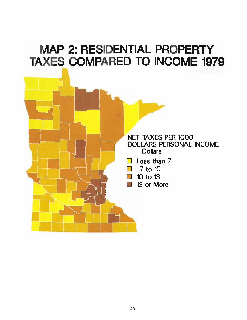
MAP 2: RESIDENTIAL PROPERTY TAXES COMPARED TO INCOME 1979

NET TAXES PER 1000 DOLLARS PERSONAL INCOME

Dollars

D Less than 7 D 7 to 10 o 10 to 13 • 13 or More

40

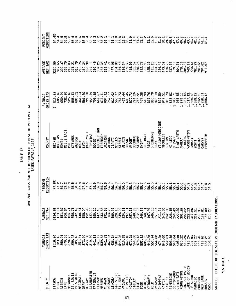
TABL

E 12

AVER

AGE

GROS

S AN

D NE

T RE

SID

ENTI

AL

HOM

ESTE

AD

PROP

ERTY

TAX

TA

XES

PAYA

BLF,

1982

AVER

AGE

AVER

AGE

PERC

ENT

AVER

AGE

AVER

AGE

PERC

ENT

COUN

TY

GROS

S TA

X NE

T TA

X RE

DUCT

ION

COUN

TY

GROS

S TA

X NE

T TA

X RE

DUCT

ION

ITAS

CA

$518

.94

$114

.81

77.9

%

BECK

ER

$ 51

6.98

$2

35.5

0 54

.4%

CO

OK

583.

46

133.

14

77.2

DO

UGLA

S 68

5.16

31

2.65

54

.4

AIT

KIN

50

0.91

15

1. 8

7 69

.7

MOW

ER

650.

69

299.

37

54.0

LA

KE

670.

55

206.

84

69.2

M

ILLE

LA

CS

732.

98

338.

79

53.8

~lAHNOMEN

378.

72

155.

71

58.9

PO

PE

525.

16

242.

83

53.8

ST

. LO

UIS

856.

48

355.

71

58.5

ST

EVEN

S 58

5.11

27

1.21

53

.6

CROW

WIN

G 58

3.40

.

242.

49

58.4

W

ASEC

A 68

0.01

31

5.79

53

.6

MAR

SHAL

L 35

1. 5

1 14

8.51

57

.8

ROCK

46

4.54

21

5.75

53

.6

GRAN

T 37

2.70

15

8.04

57

.6

LYON

55

9.60

26

0.34

53

.5

MUR

RAY

453.

80

192.

98

57.5

KA

NDIY

OHI

726.

88

338.

39

53.4

CL

EAR\

oIATE

R 31

9.69

13

7.30

57

.1

TRAV

ERSE

45

9.59

21

4.11

53

.4

FARI

BAUL

T 44

1.11

19

0.10

56

.9

DODG

E 70

8.39

33

0.49

53

.3

KITT

SON

341.

47

147.

45

56.8

KO

OCHI

CHIN

G 64

9.67

30

4.25

53

.2

MEE

KER

539.

63

233.

55

56.7

FR

EEBO

RN

611.

41

286.

34

53.2

NO

RMAN

44

1. 9

1 19

1. 6

9 56

.6

JACK

SON

604.

92

283.

41

53.1

RE

DI'10

0D

467.

93

203.

29

56.6

W

INON

A 75

2.27

35

2.71

53

.1

LINC

OLN

436.

88

190.

69

56.4

IS

AN

TI

,910

.02

427.

06

53.1

BI

G ST

ONE

504.

15

220.

15

56.3

NO

BLES

56

3.77

26

4.80

53

.0

FILU

·l0RE

54

4.06

23

9.09

56

.1

STEE

LE

751.

73

354.

49

52

.8'

\oIAD

ENA

510.

98

224.

81

56.0

W

ILKI

N 47

3.44

22

6.34

52

.2

, .j:

::.

RENV

ILLE

44

7.10

19

7.31

55

.9

BROW

N 60

3.45

28

9.33

52

.1

--'

HOUS

TON

672.

88

297.

11

55.8

W

RIGH

T 87

0.72

41

8.55

51

. 9

SIBL

EY

544.

80

2"40

.99

55.8

GO

ODHU

E 72

4.26

35

1. 5

7 51

.4

PIN

E 47

9.13

21

2.02

55

.7

STEA

RNS

753.

94

366.

26

51.4

TO

DD

557.

22

246.

76

55.7

SW

IFT

477.

38

232.

78

51.2

~10RRISON

605.

91

268.

81

55.6

BE

LTRA

MI

618.

98

301.

93

51. 2

WATON~/AN

443.

28

197.

26

55.5

RI

CE

869.

76

425.

29

51.1

PO

LK

553.

94

246.

55

55.5

SH

ERBU

RNE

880.

79

431.

23

51.0

'

WAB

ASHA

56

4.88

25

1.87

55

.4

CLAY

82

6.10

40

4.73

51

.0

CHIP

PEW

A 47

4.68

21

1. 8

1 55

.4

YELL

OW M

EDIC

INE

539.

59

264.

42

51. 0

M

ARTI

N 54

6.00

24

3.80

55

.3

NICO

LLET

94

7.51

47

3.02

50

.1

CARL

TON

542.

03

242.

80

55.2

BE

NTON

84

9.78

42

5.73

49

.9

PIPE

STO

NE

508.

58

228.

15

55.1

f>lC

LE

OD

833.

02

417.

77

49.8

CO

TTON

I400

D 54

9.04

24

6.49

55

.1

CHIS

AGO

1,01

2.71

52

9.69

47

.7

OTTE

R TA

IL

495.

40

222.

66

55.1

BL

UE

EART

H 95

5.55

50

4.31

47

.2

PENN

INGT

ON

670.

22

301.

26

55.0

AN

OKA'

" 1,

278.

10

678.

33

46.9

LA

C QU

I PA

RLE

450.

26

202.

82

55.0

OL

MST

ED

1,08

1. 5

8 58

4.86

45

.9

LAKE

OF

WOO

DS

493.

24

222.

23

54.9

W

ASHI

NGTO

N 1,

317.

21

740.

19

43.8

LE

SUE

UR

704.

83

317.

86

54.9

RA

MSE

Y 1,

360.

69

770.

13

43.4

KA

NABE

C 66

9.27

30

2.51

54

.8

SCOT

T 1,

368.

29

781.

99

42.8

HU

BBAR

D 46

2.33

20

9.41

54

.7

DAKO

TA

1,35

2.39

78

1. 6

2 42

.2

RED

LAKE

41

8.60

18

9.81

54

.7

CARV

ER

1,35

0.61

79

4.62

41

.2

ROSE

AU

338.

24

153.

80

54.5

HE

NNEP

IN

1,50

5.13

91

1.07

39

.5

CASS

56

0.43

25

5.27

54

.5

SOUR

CE:

OFF

ICE

OF

LEG

ISLA

TIV

E AU

DITO

R CA

LCUL

ATIO

NS.

"'EST

IMAT

E

From Table 12, we see significant differences in the per­centage reduction of residential gross tax bills from county to county. The state pays 77.9 percent of the average gross tax bill in Itasca county but only 39.5 percent of the average gross tax bill in Hennepin county.

Of course, Hennepin County receives more homestead credit dollars from the state per homestead than Itasca County because taxes are higher in Hennepin County. The point of the analysis that follows is that in percentage terms, the homestead credit reduces taxe'S less in high tax areas than low tax areas. This occurs because of the $650 cap on the homestead credit and the fact that more home­steads are at this maximum in high tax counties than in low tax counties.

Map 3 shows the geographic distribution of percent reduc­tion in average gross tax bills by county. Gross tax bills are re­duced the greatest amount in the six large taconite producing counties in northeastern Minnesota and in Mahnomen county. Each of these counti~s has its average gross bill reduced by more than 58 percent. Average tax bills are reduced least in the seven county metro area and in Chisago, Blue Earth and Olmstead counties, all of which re­ceive less than a 48 percent reduction in residential taxes. As we saw earlier, these are the counties with the highest residential prop­erty taxes in the state.

The percent reduction in gross residential tax bills in a taxing district is a function of the number of homesteads in the district at the homestead credit maximum and the amount of tax levies on these homesteads, and the eligibility of homesteads for other state direct property tax relief programs. For example, a county with a large number of homesteads receiving the $650 maximum homestead credit receives a smaller percentage decrease in the average gross tax bill than a county with very' few homesteads at the maximum. Counties with large numbers of homesteads eligible for the taconite homestead credit programs receive an additional decrease in the average gross tax bill.

Table 13 shows the number of homesteads at the $650 home­stead credit maximum for the seven county metro area and the 80 remaining counties in the state.

Over one-half of the homesteads in the Twin Cities metro area are currently at the $650 homestead maximum, compared to 10.3 percent of homesteads in the remainder of the state. Thus, gross tax bills are reduced less by the homestead credit in the seven county metro area than in the rest of the state.

42

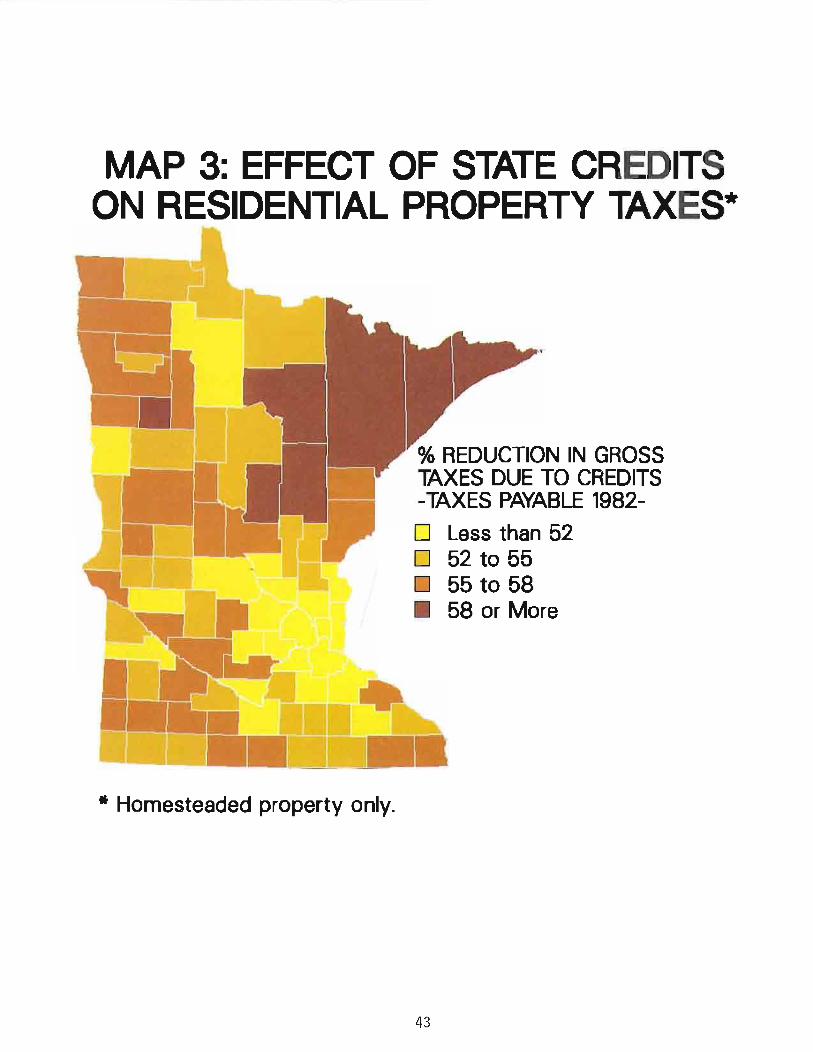
MAP 3: EFFECT OF STATE CREDITS ON RESIDENTIAL PROPERTY TAXES·

* Homesteaded property only.

% REDUCTION IN GROSS TAXES DUE TO CREDITS -TAXES PAYABLE 1982-

D Less than 52 D 52 to 55 D 55 to 58 • 58 or More

43

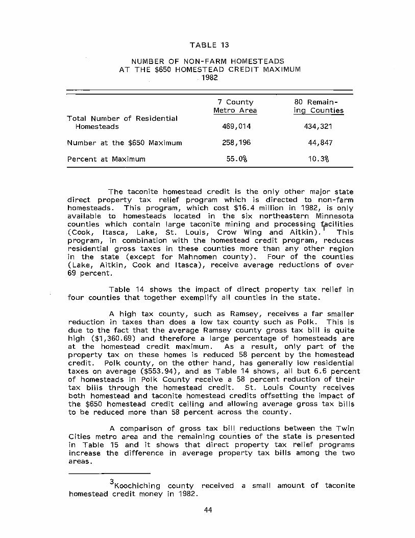
TABLE 13

NUMBER OF NON-FARM HOMESTEADS AT THE $650 HOMESTEAD CREDIT MAXIMUM

1982

7 County 80 Remain-Metro Area ing Counties

Total Number of Residential Homesteads 469,014 434,321

Number at the $650 Maximum 258,196 44,847

Percent at Maximum 55.0% 10.3%

The taconite homestead credit is the only other major state direct property tax relief program which is directed to non-farm homesteads. This program, which cost $16.4 million in 1982, is only available to homesteads located in the six northeastern Minnesota counties which contain large taconite mining and processing ~cilities (Cook, Itasca, Lake, St. Louis, Crow Wing and Aitkin). This program, in combination with the homestead credit program, reduces residential gross taxes in these counties more than any other region in the state (except for Mahnomen county). Four of the counties (Lake, Aitkin, Cook and Itasca), receive average reductions of over 69 percent.

Table 14 shows the impact of direct property tax relief in four counties that together exemplify all counties in the state.

A high tax county, such as Ramsey, receives a far smaller reduction in taxes than does a low tax county such as Polk. This is due to the fact that the average Ramsey county gross tax bill is quite high ($1,360.69) and therefore a large percentage of homesteads are at the homestead credit maximum. As a result, only part of the property tax on these homes is reduced 58 percent by the homestead credit. Pol k county, on the other hand, has generally low residential taxes on average ($553.94), and as Table 14 shows, all but 6.6 percent of homesteads in Pol k County receive a 58 percent reduction of their tax bills through the homestead credit. St. Louis County receives both homestead and taconite homestead credits offsetting the impact of the $650 homestead credit ceiling and allowing average gross tax bills to be reduced more than 58 percent across the county.

A comparison of gross tax bill reductions between the Twin Cities metro area and the remaining counties of the state is presented in Table 15 and it shows that direct property tax relief programs increase the difference in average property tax bills among the two areas.

3Koochiching county received a small amount of taconite homestead credit money in 1982.

44

TABLE 14

COMPARISON OF TAX REDUCTIONS IN FOUR COUNTIES 1982

Ramsex: st. Louis Blue Earth Polk Gross Residential Homestead Taxes $141,827,011 $49,869,281 $8,878,940 $3,590,615

Credits: Homestead 61,159,796 19,081,948 4,170,881 1,983,493 Taconite

Homestead 10,050,408 Other 394,626 25,243 22,017 8,957

Net Homestead Taxes $ 80,272,589 $20,711,682 $4,686,042 $1,598,165

Percent of Homesteads at $650 Homestead

Maximum 54.8% 14.2% 23.4% 6.6%

Average Gross Residential Tax

Bill $1,360.69 $856.48 $955.55 $553.94 Average Net Residential Tax

Bill $ 770.13 $355.71 $504.31 $246.55

Percent Reduction 43.4% 58.5% 47.2% 55.5%

Source: Office of Legislative Auditor calculations

45

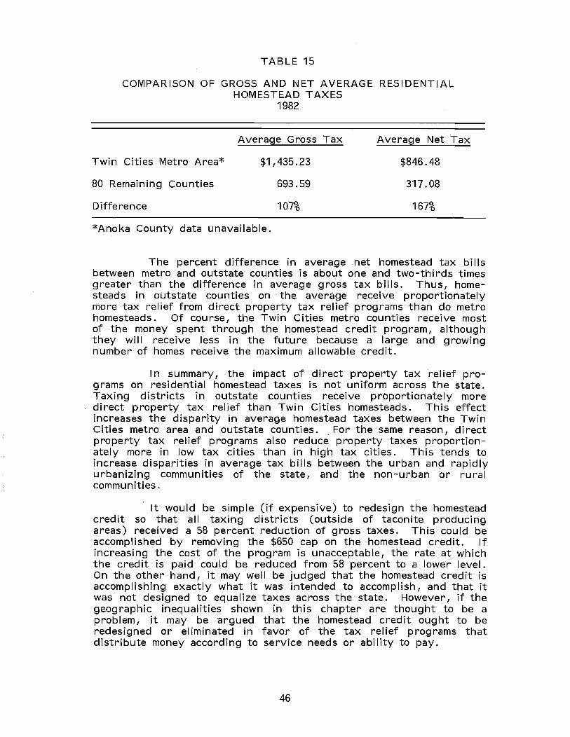
TABLE 15

COMPARISON OF GROSS AND NET AVERAGE RESIDENTIAL HOMESTEAD TAXES

Twin Cities Metro Area*

80 Remaining Counties

Difference

1982

Average Gross Tax

$1,435.23

693.59

107%

*Anoka County data unavailable.

Average Net Tax

$846.48

317.08

167%

The percent difference in average net homestead tax bills between metro and outstate counties is about one and two-thirds times greater than the difference in average gross tax bills. Thus, home­steads in outstate counties on the average receive proportionately more tax relief from direct property tax relief programs than do metro homesteads. Of course, the Twin Cities metro counties receive most of the money spent through the homestead credit program, although they will receive less in the future because a large and growing number of homes receive the maximum allowable credit.

I n summary, the impact of direct property tax relief pro­grams on residential homestead taxes is not uniform across the state. Taxing districts in outstate counties receive proportionately more direct property tax relief than Twin Cities homesteads. This effect increases the disparity in average homestead taxes between the Twin Cities metro area and outstate counties. . For the same reason, direct property tax relief programs also reduce property taxes proportion­ately more in low tax cities than in high tax cities. This tends to increase disparities in average tax bills between the urban and rapidly urbanizing communities of the state, and the non-urban or rural communities.

It would be simple (if expensive) to redesign the homestead credit so that all taxing districts (outside of taconite producing areas) received a 58 percent reduction of gross taxes. This could be accomplished by removing the $650 cap on the homestead credit. If increasing the cost of the program is unacceptable, the rate at which the credit is paid could be reduced from 58 percent to a lower level. On the other hand, it may well be judged that the homestead credit is accomplishing exactly what it was intended to accomplish, and that it was not designed to equalize taxes across the state. However, if the geographic inequalities shown in this chapter are thought to be a problem, it may be argued that the homestead credit ought to be redesigned or eliminated in favor of the tax relief programs that distribute money according to service needs or ability to pay.

46

C. PROPERTY TAXES ON FARM HOMESTEADS

Farm homesteads received over $125,000,000 in direct prop­erty tax relief in 1982. The major sources of this relief were the homestead and agricultural credit programs and this outlay represents a .substantial commitment by the state to reduce farm property taxes. First we will look at variation in property taxes on farm homesteads across the state, then the impact of state property tax relief pro­grams.

Table 16 shows the average net tax and net effective tax rate on farm homesteads for each county in 1982. The average net tax on a farm homestead ranges from a low of $106.10 in Carlton county to a high of $3,390.82 in Washington county. This wide range of average taxes is due in large measure to variation across the state in the size and value of farm homesteads.

Effective tax rates (taxes as a percent of value) are also presented in Table 16 and these, too, vary substantially across the state. While most counties have effective tax rates between .30 and .60 in 1982, four counties have tax rates greater than .95 and six counties have effective rates below .29.

Map 4 shows the geographic distribution of farm homestead effective tax rates. Counties located in the major agricultural areas of the state all fall within the .30 to .60 effective tax rate range (except Clearwater county) indicating mOdfst variation (100 percent) within the agricultural heart of the state. In contrast, wide varia­tion in effective tax rates exists in the north-central and north­eastern part of the state which is much less agriculturally oriented.

Considering the state as a whole, the variation in farm ef­fective tax rates is much greater than variation in general measures of economic well being. Table 8, presented earlier, shows that county median income varies by 137 percent across the state. Farm home­stead effective tax rates vary 2by over 900 percent from 1.79 in Lake county to .17 in Cook county. This large variation in tax burden is a product of a number of variables including differences in mill rates, property mix and eligibility of farm homesteads in the county for direct property tax relief.

1. IMPACT OF DI RECT PROPERTY TAX RELI EF PROGRAMS

Table 17 and Map 5 show the reduction in average farm homestead tax (and correspondingly, farm homestead effective tax rates) for each county in 1982. Direct property tax relief programs

1We have defined agricultural counties as counties which have 60 percent or more of property value in agricultural use.

2However, the variation in farm homestead effective tax rates for agricultural counties as a group is much more consistent with the variation in county median incomes.

47

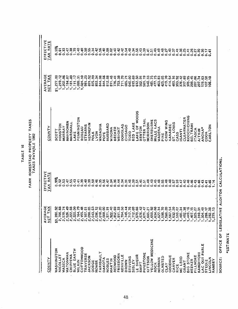
TA

BL

E

16

FAR

M

HO

MES

TEA

D

PRO

PER

TY

T

AX

ES

TA

XE

S PA

YA

,SLE

198

2

AV

ER

AG

E

EFF

EC

TIV

E

AV

ERA

GE

EFF

EC

TIV

E

CO

UN

TY

N

ET

TA

X

TA

X

RA

TE

C

OU

NT

Y

NET

T

AX

T

AX

R

AT

E

WA

SHIN

GTO

N

$3,3

90.9

2 0.

99%

S

CO

TT

$1

,277

.00

0.59

%

NIC

OL

LE

T

2,70

6.88

0.

52

HO

UST

ON

1,

219.

12

0.61

W

ASE

CA

2,

570.

74

0.53

M

UR

RA

Y

1,20

2.06

0.

33

WA

TON

WA

N

2,52

6.49

0.

47

MA

HN

OM

EN

1,18

4.07

0"

.47

CH

IPPE

WA

2,

222.

68

0.55

M

AR

SHA

LL

1,18

1.89

0.

38

BLU

E EA

RTH

2,

220.

00

0.43

LA

KE

1,11

1.17

1.

79

WIL

KIN

2,

164.

79

0.41

PE

NN

ING

TO

N

1,09

9.31

0.

40 "

C

OT

TO

NW

OO

D

2,15

5.48

0.

39

RO

SEA

U

1,02

4.10

0.

40

TR

AV

ER

SE

2,10

7.61

0.

40

STE

AR

NS

981.

23

0.50

JA

CK

SON

2,

090.

65

0.39

H

EN

NE

PIN

89

1.92

0.

55

DO

DG

E 2,

043.

63

0.50

PO

LK

875.

99

0.34

M

OW

ER

2,03

6.12

0.

46

LYO

N

853.

34

0.42

FA

RIB

AU

LT

2,

010.

20

0.35

W

AB

ASH

A

844.

98

0.56

D

AK

OTA

2,

000.

00

0.56

PO

PE

844.

66

0.40

N

OB

LE

S 1,

971.

91

0.47

H

UB

BA

RD

81

2.68

0.

98

MA

RTI

N

1,92

2.40

0.

34

WIN

ON

A

811.

46

0.62

R

EDW

OO

D

1,85

2.69

0.

36

BE

CK

ER

77

6.41

0.

40

FRE

EB

OR

N

1,81

1.33

0.

44

WR

IGH

T 75

3.38

0.

42

RE

NV

ILL

E

1,79

4.50

0.

34

DO

UG

LAS

711.

79

0.42

..J:

::>

BR

OW

N

1,74

9.44

0.

31

CH

ISA

GO

66

5.71

0.

54

CO

STE

VE

NS

1,71

7.76

0.

46

TO

DD

64

0.00

0.

49

SIB

LE

Y

1,71

2.09

0.

39

RED

LA

KE

619.

69

0.34

LE

SU

EU

R

1,"6

79.6

6 0.

51

LAK

E O

F W

OO

DS

612.

50

0.56

SW

IFT

1,

676.

42

0.45

B

EN

TO

N

562.

91

0.43

PI

PEST

ON

E

1,67

1.47

0.

51

OT

TE

R T

AIL

56

1.19

0.

39

KIT

TSO

N

1,66

5.21

0.

48

MO

RR

ISO

N

540.

33

0.41

Y

ELLO

W M

ED

ICIN

E

1,65

9.92

0.

43

SHE

RB

UR

NE

48

5.75

0.

51

RO

CK

1,

634.

80

0.45

M

ILLE

LA

CS

477.

75

0.43

N

OR

MA

N

1,62

7.34

0.

48

WA

DEN

A

463.

83

0.49

O

LMST

ED

1,59

8.70

0.

55

PIN

E

425.

65

0.48

C

LAY

1,

586.

20

0.48

C

RO

W W

ING

41

9.70

0.

27

GO

OD

HU

E 1,

567.

54

0.48

K

AN

AB

EC

414.

54"

0.43

C

AR

VE

R

1,53

2.20

0.

57

ST

. L

OU

IS

403.

16

0.37

R

ICE

1,

510.

07

0.59

C

ASS

39

3.92

0.

41

MC

LEO

D

1,49

5.34

0.

47

ISA

NT

I 37

6.42

0.

36

GR

AN

T

1,49

2.38

0.

40

CLE

AR

WA

TER

31

7.89

0.

25

BIG

ST

ON

E

1,44

9.16

0.

46

KO

OC

HIC

HIN

G

305.

95

0.41

M

EEK

ER

1,40

7.15

0.

46

BEL

TRA

MI

208.

45

0.26

FI

LLM

OR

E 1,

325.

27

0.43

IT

ASC

A

207.

86

0.27

K

AN

DIY

OH

I 1,

310.

31

0.48

A

ITK

IN

207.

74

0.20

LA

C

QU

I PA

RL

E

1,30

4.49

0.

43

AN

OK

A*

178.

63

0.36

ST

EE

LE

1,

288.

17

0.41

C

OO

K

137.

58

0.17

L

INC

OL

N

1,28

2.38

0.

46

CA

RL

TO

N

106.

10

0.41

R

AM

SEY

1,

279.

13

1.1

4

SOU

RC

E:

OFF

ICE

OF

LE

GIS

LA

TIV

E A

UD

ITO

R

CA

LC

UL

AT

ION

S.

*EST

IMA

TE

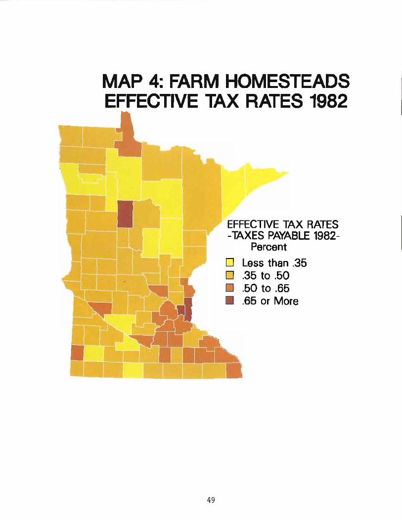
MAP 4: FARM HOMESTEADS EFFECTIVE TAX RATES 1982

49

EFFECTIVE TAX RATES -TAXES PAYABLE 1982-

Percent

o Less than .35 o .35 to .50 D .50 to .65 • . 65 or More

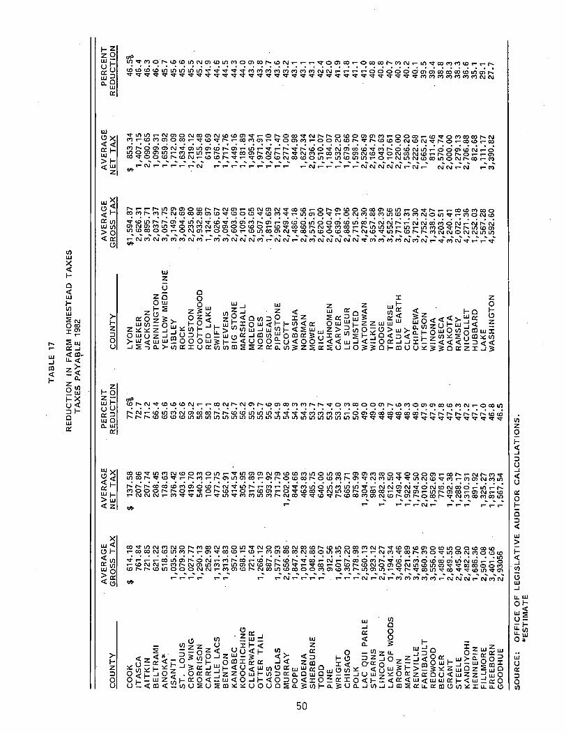
TA

BL

E 1

7

RE

DU

CT

ION

IN

FA

RM

H

OM

EST

EA

D

TA

XE

S T

AX

ES

PAY

AB

LE

198

2 ,

AV

ER

AG

E

AV

ER

AG

E

PER

CE

NT

A

VE

RA

GE

A

VE

RA

GE

PE

RC

EN

T

CO

UN

TY

G

RO

SS

TA

X

NE

T

TA

X

RE

DU

CT

ION

C

OU

NT

Y

GR

OSS

T

AX

N

ET

TA

X

RE

DU

CT

ION

CO

OK

$

614.

18

$ 13

7.58

77

.6%

LY

ON

$1

,594

.87

$ 85

3.34

46

.5%

IT

ASC

A

761.

84

207.

86

72

.7

MEE

KER

2,

626.

31

1,40

7.15

46

.4

AIT

KIN

72

1.85

20

7.74

7

1.2

JA

CK

SON

3,

895.

71

2,09

0.65

46

.3

BE

LT

RA

MI

621.

22

208.

45

66.4

PE

NN

ING

TO

N

2,03

7.37

1,

099.

31

46.0

. A

NO

KA

* 51

8.63

17

8.63

65

.6

YEL

LOW

M

EDIC

IN.E

3,

057.

75

1,65

9.92

45

.7

ISA

NT

I 1,

035.

52

376.

42

63.6

SI

BL

EY

3,

149.

29

1,71

2.09

45

.6

ST

. L

OU

IS

1,07

9.30

40

3.16

62

.6

RO

CK

3,

004.

69

1,63

4.80

45

.6

CR

OW

WIN

G

1,02

7.77

41

9.70

59

.2

HO

UST

ON

2,

235.

80

·1,2

19

.12

45

.5

MO

RR

ISO

N

1,29

0.13

54

0.33

58

.1

CO

TT

ON

WO

OD

3,

932.

86

2,15

5.48

45

.2

CA

RL

TO

N

252.

98

106.

10

58.1

R

ED

LAK

E 1,

124.

97

619.

69

44.9

M

ILLE

L

AC

S 1,

131.

42

477.

75

57.8

SW

IFT

3,

026.

67

1,67

6.42

44

.6

BE

NT

ON

1,

313.

83

562.

91

57.2

ST

EV

EN

S 3,

094.

42

1,71

7.76

44

.5

KA

NA

BE

C

957.

60

414.

54 .

56

.7

BIG

ST

ON

E

2,60

3.69

1,

449.

16

44.3

K

OO

CH

ICH

ING

69

8.15

30

5.95

56

.2

MA

RSH

ALL

2,

109.

01

1,18

1.89

44

.0

CL

EA

RW

AT

ER

72

1.64

31

7.89

55

.9

MC

LEO

D

2,66

3.65

1,

495.

34

43.9

O

TT

ER

T

AIL

1,

266.

12

561.

19

55.7

N

OB

LE

S 3,

507.

42

1,97

1.91

43

.8

CA

SS

887.

30

393.

92

55.6

R

OS

EA

U'

1,81

9.69

1,

024.

10

43.7

D

OU

GL

AS

1,57

7.93

71

1.79

54

.9

PIPE

STO

NE

2,

961.

32

1,67

1.47

43

.6

MU

RR

AY

2,

65.6

.86

. 1,

202.

06

54.8

S

CO

TT

2,

249.

44

1,27

7 .0

0 43

.2

(J"J

PO

PE

1,84

7.82

84

4.66

54

.3

WA

BA

SHA

1,

486.

18

844.

98

43.1

0

WA

DEN

A

1,01

4.28

46

3.83

54

.3

NO

RM

AN

2,

860.

56

1,62

7.34

43

.1

SHE

RB

UR

NE

1,

048.

86

485.

75

53.7

M

OW

ER

3,57

5.91

2,

036.

12

43.1

T

OD

D

1,38

1.07

64

0.00

53

.7

RIC

E

2,62

0.00

1,

510.

07

42.4

PI

NE

91

2.56

42

5.65

53

.4

MA

HN

OM

EN

2,04

0.47

1,

184.

07

42.0

W

RIG

HT

1,

601.

35

753.

38

53.0

C

AR

VE

R

2,63

9.19

1,

532.

20

41.9

C

HIS

AG

O

1,36

7.20

66

5.71

51

.3

LE S

UE

UR

2,

886.

06

1,67

9.66

41

.8

POLK

1,

778.

98

875.

99

50.8

O

LM

STE

D

2,71

5.20

1,

598.

70

41.1

LA

C

QU

I PA

RL

E

2,56

0.13

1,

304.

49

49.0

W

ATO

NW

AN

4,

278.

30

2,52

6.49

.

41.0

ST

EA

RN

S 1,

923.

12

981.

23

49.0

W

ILK

IN

3,65

7.88

2,

164.

79

40.8

L

INC

OL

N

2,50

7.27

1,

282.

38

48.9

D

OD

GE

3,45

2.39

2,

043.

63

40.8

LA

KE

OF

WO

OD

S 1

,19

4.3

4

612.

50

48.7

T

RA

VE

RSE

3,

552.

56

2,10

7.61

40

.7

BR

OW

N

3,40

6.46

1,

749.

44

48.6

B

LUE

EA

RT

H

3,71

7.65

2,

220.

00

40.3

M

AR

TIN

3,

721.

89

1,92

2.40

48

.3

CL

AY

2,

651.

31

1,58

6.20

40

.2

RE

NV

ILL

E

3,45

3.76

1,

794.

50

48.0

C

HIP

PEW

A

3,71

2.30

2,

222.

68

40 ..

1 FA

RIB

AU

LT

3,

860.

39

2,01

0.20

47

.9

KIT

TSO

N

2,75

2.24

1,

665.

21

39.5

R

EDW

OO

D

3,55

6.00

1,

852.

69

47.9

W

INO

NA

1,

338.

07

811.

46

39

.4

BE

CK

ER

1,

488.

46

776.

41

47.8

W

ASE

CA

4,

203.

51

2,57

0.74

38

.8

GR

AN

T

2,84

9.55

1,

492.

38

47.6

D

AK

OTA

3,

240.

41

2,00

0.00

3

8.3

ST

EE

LE

2,

445.

90

1,28

8.17

47

.3

RA

MSE

Y

2,07

2.18

1,

279.

13

38.3

K

AN

DIY

OH

I 2,

482.

20

1,31

0.31

47

.2

NIC

OL

LE

T

4,27

1.36

2,

706.

88

36.6

H

EN

NE

PIN

1,

686.

36

891.

92

47.1

H

UB

BA

RD

1,

252.

03

812.

68

35.1

FI

LLM

OR

E 2,

501.

08

1,32

5.27

47

.0

LAK

E 1,

567.

28

1,11

1.17

29

.1

FRE

EB

OR

N

3,40

1.66

1,

811.

33

46.8

W

ASH

ING

TO

N

4,59

2.60

3,

390.

82

27.7

G

OO

DH

UE

2,93

056

1,56

7.54

46

.5

SOU

RC

E:

OFF

ICE

OF

LE

GIS

LA

TIV

E

AU

DIT

OR

C

AL

CU

LA

TIO

NS.

*E

STIM

AT

E

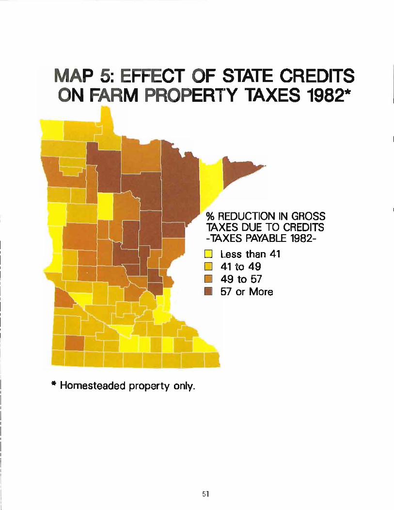
MAP 5: EFFECT OF STATE CREDITS ON FARM PROPERTY TAXES 1982*

• Homesteaded property only.

% REDUCTION IN GROSS TAXES DUE TO CREDITS -TAXES PAYABLE 1982-

D Less than 41 D 41 to 49

49 to 57 .• 57 or More

51

reduced average farm homestead taxes from 28 to 78 percent across the state in 1982. This represents a 178 percent difference in aver­age tax reductions from the highest to lowest county.

The four counties with the highest net effective tax rates (Lake, Ramsey, Washington, and Hubbard) received among the lowest percent reductions in farm homestead taxes. I n contrast, the counties with the lowest net effective tax rates generally received the greatest percentage reduction. Thus, as was the case for non-farm home­steads, there is more variation in net taxes than gross taxes on farm homesteaded property.

The agricultural credit reduces taxes most in districts with high agricultural property values. These areas are not in general high tax areas of the state. The homestead credit works the same for farm homesteads as for non-farm homesteads. It reduces taxes proportionately more in low tax areas than high tax areas. Again, we believe the question raised by this finding is whether direct property tax relief programs make sense if they reduce taxes in low tax areas more than in high tax areas, or whether there isn1t a better way to distribute property tax relief, especially in a time of budget short­ages.

52

III. DI RECT PROPERTY TAX RELI EF PROGRAMS

This chapter examines in detail the homestead credit, agri­cultural credit, and circuit breaker, Minnesota's three major direct property tax relief programs. We look at each program's history, growth, and objectives. We also evaluate the ~ffectiveness of each program and present a discussion of policy alternatives.

No attempt is made to provide a blueprint for legislative action i rather this report discusses the steps to be taken to move the system in alternative directions that may be judged desirable. In addition to policy alternatives we identify technical improvements to each program that we believe will make the programs work better. The administration of the homestead credit and circuit breaker for renters is the subject of a separate report Administration of Direct Property Relief Programs. However, the major findings of this study are summarized here. Finally, this chapter includes a brief section on the additive effects of direct property tax relief programs including the minor programs such as the wetland, native prairie, and reduced assessment credit that were otherwise not studied in detail.

A. HOMESTEAD CREDIT

The homestead credit is Minnesota's largest direct property tax relief program. In 1982, the homestead credit reduced the tax liability of homeowners by $479 million. Currently the homestead credit reduces the property taxI Of owner-occupieq housing by 58 per­cent, up to a maximum of $650. '

II n 1982, the homestead credit was figured on a maximum of 108 percent of a taxing district's 1981 levy except for school districts. A maximum appropriation was a,lso set for 1982 and 1983, which in 1982 resulted in a reduction in homestead credit payments to all taxing districts. I n some previous years the homestead credit was calculated on the non-debt levy of local units rather than the total property tax. Taxes were reduced by $479 million in 1982 by the homestead credit, but because of a series of state spending reductions, taxing districts received only $385 million. In previous years the state reimbursed taxing districts on the full amount of the homestead credit. To soften the impact of the 1982 cuts, local taxing districts were allowed to speed up property tax collections.

2An additional $16 million was paid through the taconite homestead credit. In certain iron range areas, depending on the iron ore value of the taxing district or the presence of taconite mines or electric generatjng facilities, an additional 57 or 66 percent, up to a maximum of $375 or $430 is paid by the state before the regular homestead credit is calculated. The taconite homestead credit is paid from taconite production tax receipts.

53

1. HISTORICAL GROWTH OF THE PROGRAM

Table 18 shows the annual growth in tax levies between 1967 and 1982 and the growth in the homestead credit. Over the period 1968 to 1982, total tax levies have grown over 200 percent, but the homestead credit has grown more than 500 percent. A closer look at Table 18 shows that the homestead credit has grown every year but one since its inception in 1968, and by substantial amounts between 1973 and 1974 and between 1979 and 1981. The explanation of this pattern of growth is fairly simple. In 1968 the homestead credit was equal to 35 percrnt of the property tax owed by homesteads to a maximum of $250. Effective in 1974 the credit was expanded to pay 45 percent of a homeowner's tax bill up to a maximum of $325. This explains why the cost of the homestead credit program increased 54.3 percent between 1973 and 1974, while total taxes went up about 10 per­cent during the same year. Before 1974, the cost of the homestead credit rose at about the same rate as property taxes as a whole. In 1973, 14.1 percent of all homesteads were receiving the maximum credit of $250. In 1974, these homesteads were suddenly eligible for a credit of up to $325.

Between 1974 and 1979, homestead credit expenditures grew at an annual rate ranging from 4.0 to 9.2 percent, reflecting the growth in taxes on homesteaded property and the proportion of home­steads receiving the maximum credit. By 1979, nearly 49 percent of all homesteads were receiving the $325 maximum credit and for these homeowners the homestead credit had ceased to protect against prop" erty tax increases.

In the 1979 and 1980 sessions, the legislature extended the homestead credit again. Effective in 1980, the homestead credit was increased to pay 50 percent of the tax on homesteaded property to a maximum of $550. And effective in 1981, the rate increased to 58 percent and the maximum to $650. Reflecting these increased limits, homestead credit expenditures grew 46.1 percent in 1980 and 20.4 percent in 1981. In 1982, the credit grew 7.2 percent. In 1982, 34.8 percent of homesteads were at the maximum and the homestead credit totalled $479 million. As noted on Table 18, the actual cost of the homestead credit for taxes payable in 1982 was $385 million due to late spending cuts. There are now somewhat over one million home­steads eligible to receive the homestead credit and if each received the maximum credit', (and a state appropriation covered the full obligation of the program) the cost to the state would be about $670 million a year or 39.7 percent more than the total credit in 1982. Thus, if the 58 percent rate and $650 maximum remain fixed into the future, the growth in the cost of the homestead credit will be modest compared to the increases experienced in recent years. The more than 500 percent increase in the cost of the homestead credit since 1968 is largely due to increases in homestead credit limits effective in 1974, 1980 and 1981.

11 n this year the credit went only to the non-debt levy, but this is very close to the total levy.

54

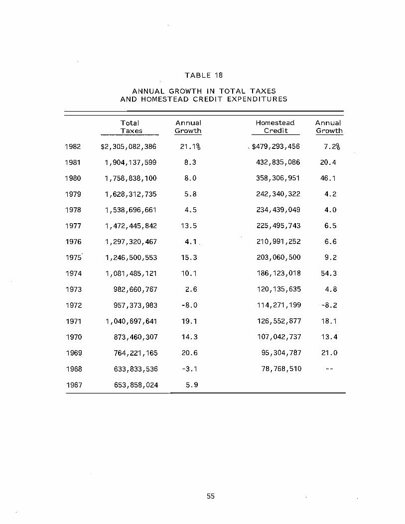
TABLE 18

ANNUAL GROWTH IN TOTAL TAXES AND HOMESTEAD CREDIT EXPENDITURES

Total Annual Homestead Annual Taxes Growth Credit Growth

1982 $2,305,082,386 21.1% ' $479,293,456 7.2%

1981 1,904,137,599 8.3 432,835,086 20.4

1980 1,758,838,100 8.0 358,306,951 46.1

1979 1,628,312,735 5.8 242,340,322 4.2

1978 1,538,696,661 4.5 234,439,049 4.0

1977 1,472,445,842 13.5 225,495,743 6.5

1976 1,297,320,467 4.1 210,991,252 6.6

1975 1,246,500,553 15.3 203,060,500 9.2

1974 1,081,485,121 10.1 186, 123,018 54.3

1973 982,660,767 2.6 120,135,635 4.8

1972 957,373,983 -8.0 114,271 , 199 -8.2

1971 1,040,697,641 19.1 126,552,877 18.1

1970 873,460,307 14.3 107,042,737 13.4

1969 764,221,165 20.6 95,304,787 21.0

1968 633,833,536 -3.1 78,768,510

1967 653,858,024 5.9

55

As a point of comparison, if the homestead credit still were limited to a maximum of $250, and if all 1,029,593 homesteads in Minnesota in 1982 received the maximum credit, the program would cost $257 million. If the maximum were $325 (as it was in 1974) and all homesteads were at the maximum, the cost would be $335 million. A $550 maximum implies a maximum program cost of $566 million. Actually, even in 1982 close to 15 percent of Minnesota homesteads received a credit of less than $200, so these figures overstate what the actual cost of the homestead credit would be if a lower maximum credit were in effect today.

Thus, the major explanation for why homestead credit costs have increased over 500 percent since 1968 is that the original pro­gram was expanded several times. I n recent years the homestead credit has been a source of concern because its cost has grown faster than state revenue, and that growth in the cost of the program depended in part on decisions taken in 4,000 local taxing districts around the state rather than in the state legislature. As we have just seen, however, the big growth in the program has resulted from legislative action that deliberately increased the rate at' which the credit is paid and the maximum credit paid.

2. PROJECTED GROWTH

Precise calculation of the cost of the homestead credit into the future is limited by the fact that 4,000 more or less independent taxing districts make budgetary decisions that can affect the exact cost of the program. Rough calculation of the cost of the program a few years into the future is not difficult however, given information on the number of eligible homesteads in the state and assumptions about the growth in this number, the number of homesteads at the maximum--these are receiving all the money they are going to get-­and assumptions about growth in taxes on homesteaded property across the state. Under the assumption that levies in cities, town, and special districts will increase the same amount in 1983 and 1984 as

. they did between 1981 and 1982 and that school district levies will increase 15 percent in 1983 and 8 percent in 1984, the Department of Finance using a Revenue Department model has estimated that the homestead credit will cost $513 million in 1983 and $532 million in 1984 compared to $479 million in 1982. Projections made independently by the House of Representatives Research Department' are in general accord with these figures. These projections can and will be refined as more is learned about actual 1983 levies.

3. OBJECTIVES OF THE HOMESTEAD CREDIT

On one level, the purpose of the homestead credit is simple: to reduce property taxes on owner-occupied property. Along with other property tax relief programs that are designed to keep property taxes low, the homestead credit has succeeded in bringing property taxes in Minnesota down to a level that is low in comparison to other states. While the general purpose and impact of the homestead credit is clear, it has a variety of other effects that may be viewed as

56

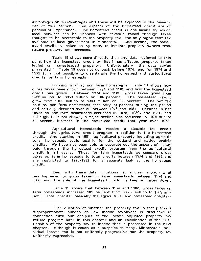
advantages or disadvantages and these will be explored in the remain­der of this section. Two aspects of the homestead credit are of paramount importance. The homestead credit is one means by which local services can be financed with revenue raised through taxes thought to be preferable to ,the property tar, the only significant tax available to local government in Minnesota. And second, the home­stead credit is looked to by many to insulate property owners from future property tax increases.

Table 19 shows more directly than any data reviewed to this point how the homestead credit by itself has affected property taxes levied on homesteaded property. Unfortunately, the data series presented in Table 19 does not go back before 1974, and for 1974 and 1975 it is not possible to disentangle the homestead and agricultural credits for farm homesteads.

Looking first at non-farm homesteads, Table 19 shows how gross taxes have grown between 1974 and 1982 and how the homestead credit has grown. Between 1974 and 1982, gross taxes grew from $466 million to $959 million or 106 percent. The homestead credit grew from $165 million to $393 million or 138 percent. The net tax paid by non-farm homesteads rose only 73 percent during the period and actually declined over-all between 1976 and 1981. Declines in net taxes on non-farm homesteads occurred in 1978, 1980, and 1981, and although it is not shown, a major decline also occurred in 1974 due to 54 percent increase in the homestead credit that year over 1973.

Agricultural homesteads receive a sizeable tax credit through the agricultural credit program in addition to the homestead credit. And starting in 1981, agricultural property including agricul­tural homesteads could qualify for the wetland and native prairie credits. We have not been able to separate out the amount of money paid through the homestead credit program from the agricultural credit in all years. Thus, for farm homesteads we compare gross taxes on farm homesteads to total credits between 1974 and 1982 and are restricted to 1976-1982 for a separate look at the homestead credit.

Even with these data limitations, it is clear enough what has happened to gross taxes on farm homesteads between 1974 and 1981 and the role of the homestead credit in keeping taxes down.

Table 19 shows that between 1974 and 1982, gross taxes on farm homesteads increased 181 percent from $95.7 million to $269 mil­lion. Total credits--basically the agricultural and homestead credits--

1The question of whether the property tax in fact places a disproportionate burden on low income taxpayers is discussed in connection with our analysis of the income adjusted property tax refund program later in this chapter and an examination of the rela­tionship of the property tax to income that is presented in the next chapter. Although it comes as a surprise to many, Minnesota's indi­vidual income tax is not uniformly progressive nor the property tax uniformly regressive.

57

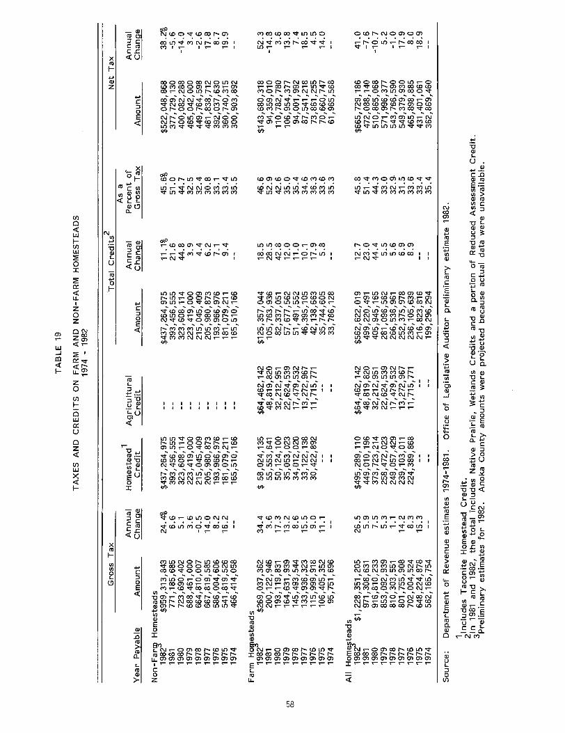
TA

BL

E 1

9

TA

XE

S A

ND

C

RE

DIT

S O

N

FARM

AN

D

NO

N-F

AR

M

HO

MES

TEA

DS

1974

-19

82

Gro

ss T

ax

Tot

al C

redi

ts2

Net

Tax

Hom

este

ad 1

As

a A

nnua

l A

gric

ultu

ral

Ann

ual

Per

cent

of

Ann

ual

Yea

r P

ayab

le

Am

ount

C

hang

e C

redi

t C

redi

t A

mou

nt

Cha

nge

Gro

ss T

ax

Am

ount

C

hang

e

Non-Far~

Hom

este

ads

1982

$9

59,3

13,8

43

24.4

%

$437

,264

,975

$4

37,2

64,9

75

11.1

%

45.6

%

$522

,048

,868

38

.2%

19

81

771

{185

,685

6.

6 39

3{45

6,55

5 39

3,45

6,55

5 21

.6

51.0

37

7,72

9,13

0 -5

.6

1980

72

3,69

0,40

2 5.

1 32

3,60

8,11

4 32

3,60

8,11

4 44

.8

44.7

40

0,08

2,28

8 -1

4.0

1979

68

8,46

1,00

0 3

.6

223,

419,

000

223,

419,

000

3.9

32

.5

465,

042,

000

3.4

19

78

664,

810,

007

-0.5

21

5,04

5,40

9 21

5,04

5,40

9 4

.4

32.4

44

9,76

4,59

8 -2

.6

1977

66

7,81

9,58

5 14

.0

205,

980,

873

205,

980,

873

6.2

30.8

46

1,83

8,71

2 17

.8

1976

58

6,00

4,60

6 8

.2

193,

966,

976

193,

966,

976

7.1

33.1

39

2,03

7,63

0 8

.7

1975

54

1,81

9,52

6 16

.2

181,

079,

211

181,

079,

211

9.4

33

.4

360,

740,

315

19.9

19

74

466,

414,

058

165,

510,

166

165,

510,

166

35.5

30

0,90

3,89

2

Farm

Ho~esteads

1982

$2

69/0

37,3

62

34.4

$

58,0

24,1

35

$64,

462,

142

$125

,357

,044

18

.5

46.6

$1

43,6

80,3

18

52.3

19

81

200,

122,

946

3.6

55

/553

,641

48

,819

,820

10

5,76

3,93

6 28

.5

52.9

94

,359

,010

-1

4.8

1980

19

3, 1

19 , 8

31

17.3

50

,124

,100

32

,212

,951

82

,337

/051

42

.8

42.6

11

0,78

2,78

0 3

.6

U"I

19

79

164,

631,

939

13.2

35

,053

,023

22

,624

,539

57

,677

,562

12

.0

35.0

10

6/95

4,37

7 13

.8

(Xl

1978

14

5,49

3,54

4 8

.6

34,0

12{0

20

17,4

79,5

32

51,4

91/5

52

11.0

35

.4

94,0

01,9

92

7.4

19

77

133,

936/

323

15.5

33

,122

,138

13

,272

,967

46

,395

,105

10

.1

34.6

87

,541

,218

18

.5

1976

11

5,99

9,91

8 9

.0

30,4

22/8

92

11,7

15,7

71

42,1

38,6

63

17.9

36

.3

73,8

61,2

55

4.5

19

75

106,

405/

352

11.1

35

,744

,605

5

.8

33.6

70

/660

,747

14

.0

1974

95

/751

/696

33

/786

,128

35

.3

61/9

65/5

68

All

Hom~teads

1982

$1

/228

/351

,205

26

.5

$495

,289

/110

$6

4{46

2,14

2 $5

62,6

22,0

19

12.7

45

.8

$665

,729

,186

41

.0

1981

97

1/30

8/63

1 5

.9

449,

010/

196

48,8

19,8

20

499,

220,

491

23.0

51

.4

472,

088,

140

-7.6

19

80

916,

810,

233

7.5

37

3,72

3,21

4 32

,212

,951

40

5,94

5/16

5 44

.4

44.3

51

0,86

5,06

8 -1

0.7

1979

85

3/09

2,93

9 5.

3 25

8,47

2,02

3 22

,624

,539

28

1,09

6,56

2 5~5

33.0

57

1,99

6,37

7 5

.2

1978

81

0,30

3,55

1 1.

1 24

9,05

7,42

9 17

,479

,532

26

6,53

6,96

1 5

.6

32.9

· 54

3,76

6,59

0 -1

.0

1977

80

1,75

5/90

8 14

.2

239,

103,

011

13,2

72,9

67

252,

375,

978

6.9

31

.5

549,

379,

930

17.9

19

76

702,

004,

524

8.3

224,

389,

868

11,7

15,7

71

236,

105,

639

8.9

33

.6

465,

898/

885

8.0

19

75

648,

224/

878

15.3

21

6,82

3,81

6 33

.4

431,

401,

061

18.9

19

74

562,

165/

754

199,

296/

294

35.4

36

2,86

9,46

0

Sou

rce:

D

epar

tmen

t of

Rev

enue

est

imat

es 1

974-

1981

. O

ffic

e of

Leg

isla

tive

Aud

itor

pre

lim

inar

y es

tim

ate

1982

.

~Inc

lude

s T

acon

ite

Hom

este

ad

Cre

dit.

31

n 19

81

and

1982

, th

e to

tal

incl

udes

Nat

ive

Pra

irie

, W

etla

nds

Cre

dits

and

a p

orti

on o

f R

educ

ed A

sses

smen

t C

redi

t.

Pre

lim

inar

y es

tim

ates

for

198

2.

Ano

ka C

ount

y am

ount

s w

ere

proj

ecte

d be

caus

e ac

tual

dat

a w

ere

unav

aila

ble.

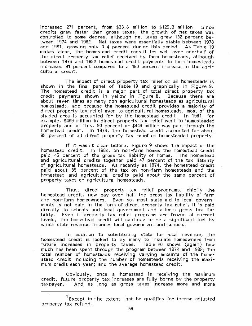
increased 271 percent, from $33.8 million to $125.3 million. Since credits grew faster than gross taxes, the growth of net taxes was controlled to some degree, although net taxes grew 132 percent be­tween 1974 and 1982. Net taxes were essentially stable between 1978 and 1981, growing only 0.4 percent during this period. As Table 19 makes clear, the homestead credit constitutes well over one-half of the direct property tax relief received by farm homesteads, although between 1976 and 1982 homestead credit payments to farm homesteads increased 91 percent compared to a 450 percent increase in the agri­cultural credit.

The impact of direct property tax relief on all homesteads is shown in the final panel of Table 19 and graphically in Figure 9. The homestead credit is a major part of total direct property tax credit payments shown in yellow in Figure 8. Because there are about seven times as many non-agricultural homesteads as agricultural homesteads, and because the homestead credit provides a majority of direct property tax relief even to agricultural homesteads, most of the shaded area is accounted for by the homestead credit. I n1981, for example, $499 million in direct property tax relief went to homesteaded property and of this, 90 percent or $449 million was paid through the homestead credit.· In 1976, the homestead credit accounted for about 95 percent of all direct property tax relief on homesteaded property.

If it wasn't clear before, Figure 9 shows the impact of the homestead credit. In 1982, on non-farm homes the homestead credit paid 46 percent of the gross tax liability of homes. The homestead and agricultural credits together paid 47 percent of the tax liability of agricultural homesteads. As recently as 1974, the homestead credit paid about 35 percent of the tax on non-farm homesteads and the homestead and agricultural credits paid about the same percent of property taxes on agricultural homesteads.

Thus, direct property tax relief programs, chiefly the homestead credit, now pay over half the gross tax liability of farm and non-farm homeowners. Even so, most state aid to local govern­ments is not paid in the form of direct property tax relief, it is paid directly to schools and local government and affects gross tax lia­bility. Even if property tax relief programs are frozen at current levels, the homestead credit will continue to be a significant tool by which state revenue finances local government and schools.

In addition to substituting state for local revenue, the homestead credit is looked to by many to insulate homeowners from future increases in property taxes. Table 20 shows (again) how much has been spent through the program between 1972 and 1982; the total number of homesteads receiving varying amounts of the home­stead credit including the number of homesteads receiving the maxi­mum credit each year; and the average homestead credit.

Obviously, once a homestead is receiving the maximum credit, fLtfure property tax increases are fully borne by the property taxpayer. And as long as g ross taxes increase more ,and more

1 Except to 'the extent that he qualifies for income adjusted property tax refund.

59

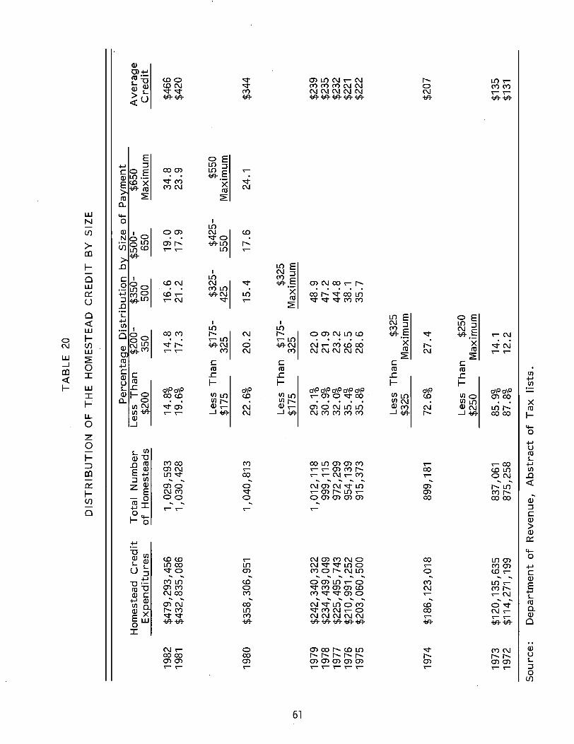
TA

BL

E

20

DIS

TR

IBU

TIO

N

OF

TH

E

HO

MES

TEA

D

CR

ED

IT

BY

SIZ

E

Per

cent

age

Dis

trib

utio

n b~

Siz

e of

Pa~ment

Hom

este

ad

Cre

dit

T

otal

N

umbe

r L

ess

Tha

n $2

00-

$350

-$5

00-

$650

A

vera

ge

Exp

endi

ture

s of

Hom

este

ads

$200

35

0 50

0 65

0 M

axim

um

Cre

dit

1982

$4

79,2

93,4

56

1,02

9,59

3 14

.8%

14

.8

16.6

19

.0

34.8

$4

66

1981

$4

32,8

35,0

86

1,03

0,42

8 19

.6%

17

.3

21.2

17

.9

23.9

$4

20

Les

s T

han

$175

-$3

25-

$425

-$5

50

$175

32

5 42

5 55

0 M

axim

um

1980

$3

58,3

06,9

51

1,04

0,81

3 22

.6%

20

.2

15.4

17

.6

24.1

$3

44

Les

s T

han

$175

-$3

25

. O

'l

$175

32

5 M

axim

um

--'

1979

$2

42,3

40,3

22

1,01

2,11

8 29

.1%

22

.0

48.9

$2

39

1978

$2

34,4

39,0

49

999,

115

30.9

%

21.9

47

.2

$235

19

77

$225

,495

,743

97

2,29

9 32

.0%

23

.2

44.8

$2

32

1976

$2

10,9

91,2

52

954,

139

35.4

%

26.5

38

.1

$221

19

75

$203

,060

,500

91

5,37

3 35

.8%

28

.6

35.7

$2

22

Les

s T

han

$325

$3

25

Max

imum

1974

$1

86,1

23,0

18

899,

181

72.6

%

27.4

$2

07

Les

s T

han

$250

$2

50

Max

imum

1973

$1

20,1

35,6

35

837,

061

85.9

%

14.1

$1

35

1972

$1

14,2

71,1

99

875,

258

87.8

%

12.2

$1

31

Sou

rce:

D

epar

tmen

t of

Rev

enue

, A

bst

ract

of

Tax

lis

ts.

homesteads will be lIat the maximum ll unless the maximum credit is regularly increased. The maximum homestead credit remained at $325 between 1974 and 1979. During this period, as Table 20 shows, the number of homesteads receiving the maximum credit increased from 27.4 percent to 48.9 percent. Subsequently, the maximum was in­creased to $550, then to $650. The $650 maximum has been in effect since 1981. In 1981, 23.9 percent of all homesteads were at the maximum. As Table 20 shows, the number of homesteads at the maximum grew to 34.8 percent in 1982.

There is wide variation across the state in the average homestead credit paid and the percent of homesteads at the maximum. Where taxes are high (because of high residential property values, high mill rates or both) more homesteads are at the maximum. In general, taxes are higher in the Twin Cities metropolitan area than in the balance of the state for reasons already discussed. Table 21 compares the seven county Twin Cities area to the balance of the state on the size distribution of the homestead credit.

Table 21 shows the extent of the difference between the Twin Cities area and the remaining 80 counties of the state in the number of homes receiving various levels of the homestead credit including the percent receiving the maximum credit. As 21 shows, 55 percent of homes in the seven county Twin Cities metropolitan area are at the maximum compared to 17 percent of the rest of the state. Only one percent of the homes in the seven county area receive less than $200 in homestead credit (meaning their gross tax is less than $345) while 27 percent of homes outside the seven county area receive a homestead credit less than $200.

Thus, over a third of all homes state-wide and over half of the homes in the Twin Cities are at the maximum. Homes just at the maximum experience the largest percentage increase in property taxes when taxes go up. Homes under the maximum have 58 percent of any tax increase paid for by the state until they reach the maximum.

As homestead taxes rise about the point where they receive the maximum credit, the impact of the homestead credit in lowering taxes diminishes. Elimination of the homestead credit therefore affects taxes on a $200,000 home less than on a $100,000 home in the same location.

I n summary, as fast as the homestead credit program has grown since 1968 and especially in the late 1970s, over a third of homesteads across Minnesota, over one-half in the Twin Cities metro­politan area and over 60 percent in Hennepin county receive the maximum allowable credit and are no longer insulated against property tax increases driven by increased local budgets.

4. ADMINISTRATION OF THE HOMESTEAD CREDIT: DETERMINING ELIGI BI LITY

Legislative reference to the homestead credit is part of the state1s property classification laws; payment of a homestead credit

62

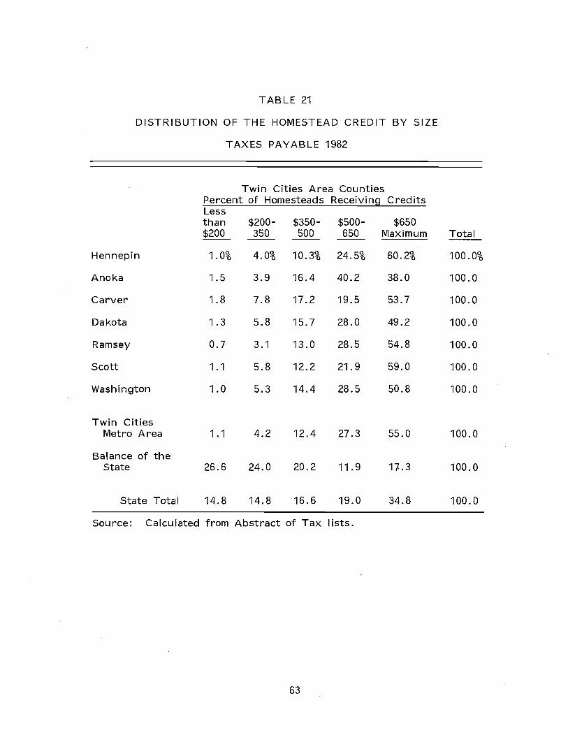
TABLE 21

DISTRIBUTION OF THE HOMESTEAD CREDIT BY SIZE

TAXES PAYABLE 1982

Twin Cities Area Counties Percent of Homesteads Receiving Credits Less than $200- $350- $500- $650 $200 350 500 650 Maximum Total

Hennepin 1.0% 4.0% 10.3% 24.5% 60.2% 100.0%

Anoka 1.5 3.9 16.4 40.2 38.0 100.0

Carver 1.8 7.8 17.2 19.5 53.7 100.0

Dakota 1.3 5.8 15.7 28.0 49.2 100.0

Ramsey 0.7 3.1 13.0 28.5 54.8 100.0

Scott 1.1 5.8 12.2 21.9 59.0 100.0

Washington 1.0 5.3 14.4 28.5 50.8 100.0

Twin Cities Metro Area 1.1 4.2 12.4 27.3 55.0 100.0

Balance of the State 26.6 24.0 20.2 11.9 17..3 100.0

State Total 14.8 14.8 16.6 19.0 34.8 100.0

Source: Calculated from Abstract of Tax lists.

63

follows from recelvmg a homestead classification. There is no "Home­stead Credit Act" expressing legislative intent, program definitions, guidelines for administrative rules, or local government and state agency responsibilities and authority. Though there is no explicit definition in statute of what constitutes a homestead, a homestead has come to mean any real property that is occupied and used by the owner on January 2 of the assessment year. I n addition, any real property that was not used for the purpose of a homestead on the January 2 assessment date, but was used for the purpose of a home­stead on the following June 1 could be classified as a mid-year home­stead for the last half of that year and would qualify for one-half of the homestead credit. Furthermore, it is assumed the Legislature intends that a property owner be given the benefits of a homestead in only one place.

The establishment of criteria to define ownership and occu­pancy has largely evolved from decisions of the Department of Reve­nue and from judgments rendered by the Minnesota Tax Court and the Attorney General. What has emerged is a practical construction of the statutes that establishes ownership and occupancy criteria that can be applied in determining homestead status.

(1) Ownership is determined by such documents as:

Warranty Deed Contract for Deed Certificate of Real Estate Value Proof of Inheritance Homestead Declaration Card

(2) Occupancy is evidenced by:

An owner's occupancy of the property on January 2. Although the January 2 date is generally required for occupancy, the courts have focused on the owner's intent, recog-

- nizing that the owner may not always be physically present on January 2.

An owner's intent to make the property his principal dwelling. By implication this means the owner has only one homestead.

Although the laws and policies governing the homestead classification establish some objective guidelines for determining home­stead status, their application can require subjective judgment. As a result, it is possible for residential properties to be misclassified as homesteads because of inconsistent interpretation and application of the homestead definition by the assessors. This can create variations within and among counties and also lead to assessors being in conflict with local Boards of Review, the Department of Revenue, and the Minnesota Tax Court.

64

I n addition, the system lacks standardized administrative requirements and, as a result, there is variation among the counties in homestead classification procedure, documentation, record keeping , and data processing. For example, while some counties tend to rely on mechanical or computerized methods, other counties rely more on personal knowledge and familiarity with their assessment district. While both systems have strengths and weaknesses, the lack of uni­formity presents significant problems for documenting and verifying information. Because these systems are so diverse, misclassified homesteads can go unnoticed for many years, if not indefinitely.

Local costs associated with administrating the homestead classification are also becoming burdensome for many counties. For example, during a meeting with the Legislative Committee of the Minnesota Association of Assessing Officers, we were told that admin­istrative costs directly associated with making and verifying homestead classifications could exceed 20 percent of the total assessor1s office budget in many counties. I n Hennepin County, the cost of mailing homestead declaration cards alone, was over $32,000 per year.

Administrative costs also have indirect impacts. Several counties indicated to us that the time and resources required to make homestead classifications greatly affects the time available to assess the value of property. To the extent assessors are not able to devote sufficient time to making assessments, the quality of those assessments may be adversely affected.

The Department of Revenue has broad legal authority over the state's property tax system. I n practice however, the department currently limits administration of homestead credits to the training and licensing of assessors and the evaluation and verification of aggregate credit amounts payable to local taxing jurisdictions. At no point in the classification process does the department systematically record, evaluate, or audit individual property classifications and credit eligibility.

The Department of Revenue is currently writing rules on homestead classification. I n addition to providing rules that would more precisely define property ownership and occupancy, the depart­ment is also exploring the feasibility of establishing rules to require the use of standardized forms and documentation for all homesteaded property in the state.

Although such a policy may appear to be contrary to the Department of Revenue's current decentralized role in overseeing the property tax system, the department has often centralized certain aspects of the system when it felt it would be beneficial to the state. For example, in recent years the department has found it necessary to standardize property tax statements, valuation notices, and certifi­cat~s of real estate value. Therefore, any degree of standardization of the homestead classification procedures would be consistent with current general state policy.

I n another report, Administration of Direct Property Tax Relief Programs, we consider options for improving the. administration of the homestead classification and credit prog ram. We suggest that

65

the Legislature and the Department of Revenue consider changes such as the following:

• Adopt an explicit definition of homestead and homestead credit eligibility.

• Establish firm filing dates for when a full or mid-year homestead application can be made.

• Require all assessors to inform new homeowners of homestead law, policies, and application procedures.

• Require that a definition of a homestead be included on all application forms and renewal cards.

• Require all property ownership contracts to be recorded with the county auditor, including all contracts for deed.

If the homestead credit is maintained, the program, which represents over 12 percent of annual general fund expenditures, should be administered with more precise and uniform standards and tighter controls. I n our judgment it is currently impossible for the state and local and county assessors to systematically audit and verify homestead classifications and therefore homestead credit eligibility. Although we have not quantified the number of misclassified residential properties, the fact remains that the current system inhibits effective and efficient auditing. A program that is as important and expensive as the homestead credit should not, in our view, be left without proper administrative controls and safeguards to ensure that its dollars are going only to those who are legally eligible to receive them. Again, we consider these issues more fully in another report, Administration of Direct Property Tax Relief Programs.

5. POLICY ALTERNATIVES

The homestead credit is a mechanism that could protect taxpayers against future property tax increases but so are a variety of other tax relief mechanisms either in place or potentially available. The question of whether the homestead credit is the preferred mecha­nism to soften property tax increases, or whether property taxes should be allowed to rise, or whether some other means should be chosen to control taxes depends on how the characteristics of each are evaluated in the political process.

The homestead credit provides something akin to across the board property tax relief to home owners. Aid is distributed at a flat rate of 58 percent to a maximum of $650. Thus, the homestead credit is only income-sensitive to a rough degree. And unlike school aids and to some extent local government aid, the homestead credit does not provide aid in a way that is tied to local need or local tax effort.

66

In our judgement, the questions boil down to these:

• Should the homestead credit be relied upon to insulate homeowners from increases in the property tax?

• To what extent should local services be financed through the homestead credit instead of property taxes or local government aid and school aids?

• Should an income-sensitive tax credit--perhaps it could be called a homestead credit--be chosen as a better tool for distributing scarce state property tax relief dollars than the present homestead credit?

• Should the homestead credit as it exists be changed in other ways? Should the rate or maximum be raised or lowered?

On the basis of the foregoing discussion and presentation of data, we have concluded that the homestead credit is accomplishing what it was designed to do: keep residential property taxes in Minnesota low and substitute state revenue for local (property tax) revenue as a means to finance local services. However, the homestead credit totalled $479 million in 1982 and the cost will rise in the future unless deliberate action is taken to limit cost increases that are built into the program.

The state1s fiscal situation in 1983, and prospects for the next few years are less promising than the conditions that prevailed through most of the 1970s when revenue growth driven by economic expansion and inflation permitted major increases in the homestead credit program. State revenue is now not growing fast enough to finance the built in growth of the homestead credit much less any liberalization of the program1s benefits. Minnesota is faced a shortage of money, and since three-fourths of the state budget is returned to local government in one form or another, it is in these programs that the legislature will need to look if significant savings are to be found.

In this light, it is possible that the homestead credit will be looked at as a program that can be cut or even eliminated because it provides property tax relief broadly rather than concentrating relief in districts with low property wealth or a high level of services needs, or distributing relief directly to taxpayers with high property taxes in relation to income. These alternatives are, essentially those presented by the school aid, local government aid, and circuit breaker programs. Focusing property tax relief more precisely may be viewed with increased favor in an era of scarce resources.

I n any case, we believe it is useful to look at possible changes in the homestead credit and their advantages and disadvan­tages. One thing is clear: If changes are made in the way a fixed amount of money is spent, there will be winners and losers, and the option of providing increased aid to some while holding all harmless seems less possible than in the past when major reforms were under­taken in the property tax system.

67

Homestead Credit Options

I. Distribute all or part of the money now going to school districts and local government via the homestead credit through the school aid and local government aid programs.

The homestead credit distributes property tax relief in a broad fashion. School aid and local government aid programs are designed to provide aid to districts with relatively high service re­quirements and relatively low property valuation. Thus, they do more than simply substitute state for local revenue. ThiY are spend­ing programs calculated to accomplish specific objectives.

I n the case of school aid, an increasing number of districts are projected to be ineligible for state foundation aid because the state mandated local levy has been increased without a compensating increase in the state foundation aid formula.

If aid paid to school districts through the homestead credit program were paid through the foundation aid program, this problem would be alleviated to some extent. The part of the homestead credit going to other local taxing districts could be paid to them through local government aid programs.

While the shape of school and local government aid programs for the future will be worked out by the 1983 legislature, and no suggestions are provided here concerning how this should be done, the general option of distributing property tax relief through these aid programs stands as a major alternative to the homestead credit. A change in the classification system lowering the assessment rates of homesteaded property could be made at the same time in order to offset the fact that school and local government aid provides relief to all property taxpayers rather than just homeowners. Another idea that has been suggested is for the state to assume the entire cost of the foundation aid program by eliminating the mandatory 26 mill foundation levy at the same time the homestead credit is abolished.

2. Distribute all or part of the homestead credit through the circuit breaker program. I n effect, change the homestead credit so that it is income­sensitive and state administered.

We have identified a number of administrative weaknesses in the homestead credit. These may be viewed as a sufficient justifica­tion for changing the way in which a half-billion dollars a year is spent through the homestead credit. One option is to assume state administration of the homestead credit by incorporating it into the income tax system.

1This is not to deny that there are many who would like to see major changes in these programs, nor to suggest that such changes should not be made.

68

This is how the circuit breaker program for homeowners is administered. Actually, the circuit breaker program for homeowners could accurately be called an income adjusted homestead credit. The current program for homeowners under 65 years of age now distrib-' utes only about $29 million compared to $63 million in 1979, and com­pared to $1.2 billion in school aid and $479 million in the homestead credit. One reason the circuit breaker refund for homeowners has dried up is that the homestead credit has been increased and, within limits, there is a dollar for dollar substitution between th.e programs. The homestead credit is deducted in the process of computing indi­vidual property tax refunds. Because of this fact, any limit on expenditures through the homestead credit that affects individual tax bills will result in more money being spent through the property tax refund for homeowners. Elsewhere we discuss the implications for the circuit breaker for limits on the homestead credit.

A variety of specific proposals can be debated. Our point here is that a second major option for the homestead credit is to make it income-sensitive. As with all proposals, some people will benefit and others will lose if a fixed amount of money is spent in a new way. The homestead credit program is popular and will not be easy to scale back or eliminate, but even if it is just not expanded, more money will be spent through the circuit breaker in the future if property taxes go up in relation to income. The circuit breaker could also be indexed against inflation in order to protect against what has happened to it because of inflation during the last few years.

3. Reduce the allowable maximum on the homestead credit, now $650.

If the homestead credit maximum were $550 instead of $650, the cost in 1982 would have been about $49 million less than it was. While this contributes to a solution of the state's money problem, data reviewed earlier show that money would be disproportionately taken from high tax areas, cities rather than outlying areas across the state, and the Twin Cities metro area rather than the balance of the state.

4. Reduce the homestead credit rate, now 58 percent.

This would also save money but at the expense of low tax rather than high tax areas (assuming the $650 maximum was kept). The homestead credit now pays 58 percent of the gross tax on owner­occupied property no matter how low the tax is. Low tax areas benefit from this feature and would lose under any plan to lower the homestead credit rate from 58 percent.

5. Keep the current rate and maximum but exempt a minimum tax from the homestead credit. This minimum could be expressed as a flat dollar amount or a fraction of (equalized) assessed or market value and could reflect the part of prop­erty tax that mainly serves property rather than people.

69

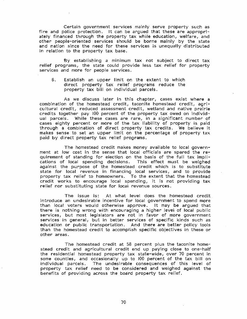
Certain government services mainly serve property such as fire and police protection. It can be argued that these are appropri­ately financed through the property tax while education, welfare, and other people-oriented services should be borne mainly by the state and nation since the need for these services is unequally distributed in relation to the property tax base.

By establishing a minimum tax not subject to direct tax relief programs, the state could provide less tax relief for property services and more for people services.

6. Establish an upper limit on the extent to which direct property tax relief programs reduce the property tax bill on individual parcels.

As we discuss later in this chapter, cases exist where a combination of the homestead credit, taconite homestead credit, agri­cultural credit, reduced assessment credit, wetland and native prairie credits together pay 100 percent of the property tax owed on individ­ual parcels. While these cases are rare, in a significant number of cases eighty percent or more of the tax liability of property is paid through a combinatioh of direct property tax credits. We believe it makes sense to set an upper limit on the percentage of property tax paid by direct property tax relief programs.

The homestead credit .makes money available to local govern­ment at low cost in the sense that local officials are spared the re­quirement of standing for election on the basis of the full tax impli­cations of local spending decisions. This effect must be weighed against the purpose of the homestead credit which is to sUbstitute state for local revenue in financing local services, and to provide property tax relief to homeowners. To the extent that the homestead credit works to encourage local spending, it is not providing tax relief nor substituting state for local revenue sources.

The issue is: At what level does the homestead credit introduce an undesirable incentive for local government to spend more than local voters would otherwise approve. It may be argued that there is nothing wrong with encouraging a higher level of local public services, but most legislators are not in favor of more government services in general, but in better services of specific kinds such as education or public transportation. And there are better policy tools than the homestead credit to accomplish specific objectives in these or other areas.

The homestead credit at 58 percent plus the taconite home­stead credit and agricultural credit end up paying close to one-half the residential homestead property tax state-wide, over 70 percent in some counties, and occasionally up to 100 percent of the tax bill on individual parcels. The undesirable consequences of this level of property tax relief need to be considered and weighed against the benefits of providing across the board property tax relief.

70

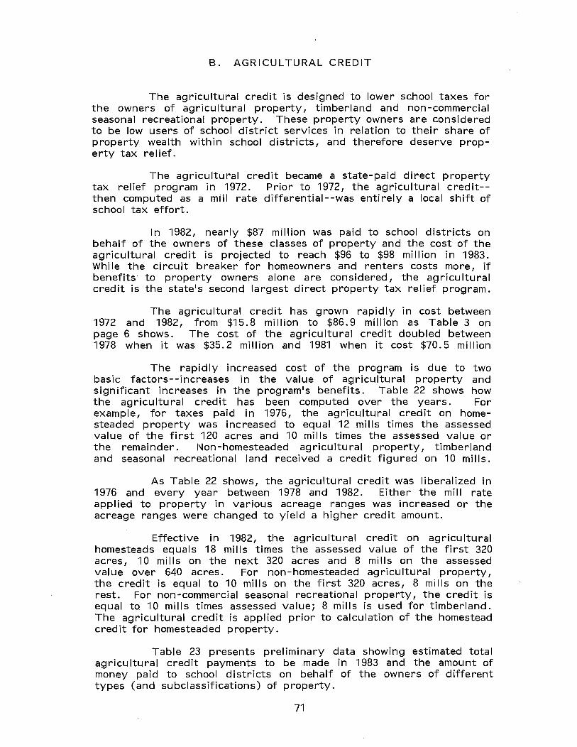
B. AGRICULTURAL CREDIT

The agricultural credit is designed to lower school taxes for the owners of agricultural property, timberland and non-commercial seasonal recreational property. These property owners are considered to be low users of school district services in relation to their share of property wealth within school districts, and therefore deserve prop­erty tax relief.

The agricultural credit became a state-paid direct property tax relief program in 1972. Prior to 1972, the agricultural credit-­then computed as a mill rate differential--was entirely a local shift of school tax effort.

In 1982, nearly $87 million was paid to school districts on behalf of the owners of these classes of property and the cost of the agricultural credit is projected to reach $96 to $98 million in 1983. While the circuit breaker for homeowners and renters costs more, if benefits to property owners alone are considered, the agricultural credit is the state's second largest direct property tax relief program.

The agricultural credit has grown rapidly in cost between 1972 and 1982, from $15.8 million to $86.9 million as Table 3 on page 6 shows. The cost of the agricultural credit doubled between 1978 when it was $35.2 million and 1981 when it cost $70.5 million

The rapidly increased cost of the program is due to two basic factors--increases in the value of agricultural property and significant increases in the program's benefits. Table 22 shows how the agricultural credit has been computed over the years. For example, for taxes paid in 1976, the agricultural credit on home­steaded property was increased to equal 12 mills times the assessed value of the first 120 acres and 10 mills times the assessed value or the remainder. Non-homesteaded agricultural property, timberland and seasonal recreational land received a credit figured on 10 mills.

As Table 22 shows, the agricultural credit was liberalized in 1976 and every year between 1978 and 1982. Either the mill rate applied to property in various acreage ranges was increased or the acreage ranges were changed to yield a higher credit amount.

Effective in 1982, the agricultural credit on agricultural homesteads equals 18 mills times the assessed value of the first 320 acres, 10 mills on the next 320 acres and 8 mills on the assessed value over 640 acres. For non-homesteaded agricultural property, the credit is equal to 10 mills on the first 320 acres, 8 mills on the rest. For non-commercial seasonal recreational property, the credit is equal to 10 mills times assessed value; 8 mills is used for timberland. The agricultural credit is applied prior to calculation of the homestead credit for homesteaded property.

Table 23 presents· preliminary data showing estimated total agricultural credit payments to be made in 1983 and the amount of money paid to school districts on behalf of the owners of different types (and subclassifications) of property.

71

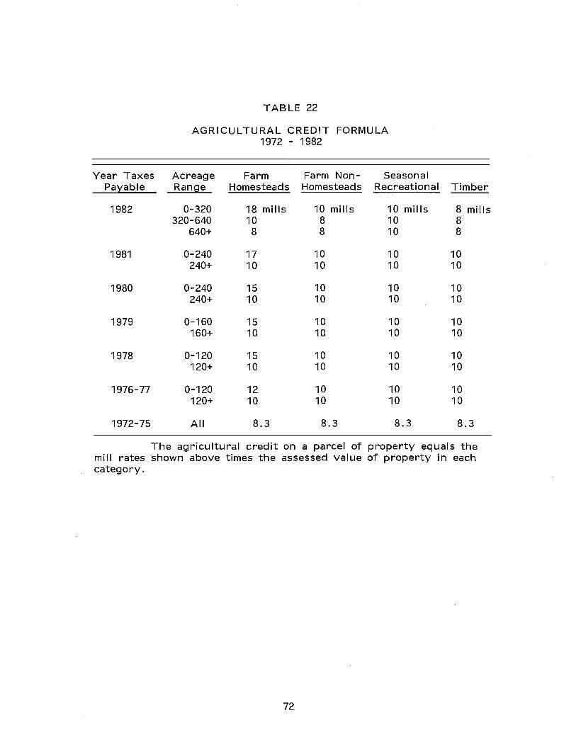
TABLE 22

AGRICULTURAL CREDIT FORMULA 1972 - 1982

Year Taxes Acreage Farm Farm Non- Seasonal Payable Range Homesteads Homesteads Recreational Timber

1982 0-320 18 mills 10 mills 10 mills 8 mills 320-640 10 8 10 8

640+ 8 8 10 8

1981 0-240 17 10 10 10 240+ 10 10 10 10

1980 0-240 15 10 10 10 240+ 10 10 10 10

1979 0-160 15 10 10 10 160+ 10 10 10 10

1978 0-120 15 10 10 10 120+ 10 10 10 10

1976-77 0-120 12 10 10 10 120+ 10 10 10 10

1972-75 All 8.3 8.3 8.3 8.3

The agricultural credit on a parcel of property equals the mill rates shown above times the assessed value of property in each category.

72

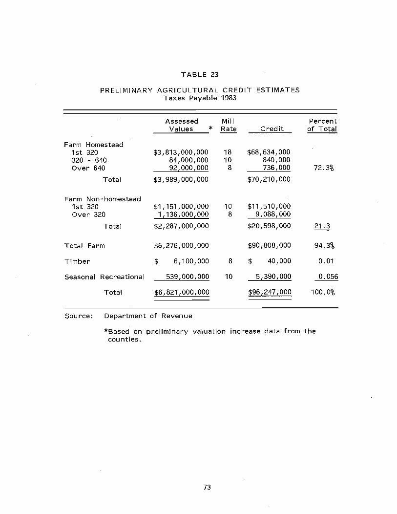
TABLE 23

PRELIMINARY AGRICULTURAL CREDIT ESTIMATES Taxes Payable 1983

Assessed Mill Percent Values * Rate Credit of Total

Farm Homestead 1st 320 $3,813,000,000 18 $68,634,000 320 - 640 84,000,000 10 840,000 Over 640 92£000,000 8 736,000 72.3%

Total $3,989,000,000 $70,210,000

Farm Non-homestead 1st 320 $1,151,000,000 10 $11,510,000 Over 320 1£136£000,000 8 9,088,000

Total $2,287,000,000 $20,598,000 21.3

Total Farm $6,276,000,000 $90,808,000 94.3%

Timber $ 6,100,000 8 $ 40,000 0.01

Seasonal Recreational 539,000£000 10 5,390£000 0.056

Total $6£821,000,000 $96£247£000 100.0%

Source: Department of Revenue

*Based on preliminary valuation increase data from the counties.

73

The agricultural credit is projected to cost $96.2 million in 1983 by the Department of Revenue, up from about $87 million in 1982. As Table 23 shows, 72.3 percent of the agricultural credit is paid on behalf of agricultural homesteads, 21 percent on agricultural non-homesteads, 0.1 percent on timberland and 5.6 percent on seasonal recreational property. As Table 23 makes clear, this is due to the distribution of assessed values across these property classes, and the fact that the mill rate on which the credit is figured is highest for the first 320 acres of agricultural homesteads.

Future changes in agricultural credit expenditures depend mainly on what happens to the market value and thus the assessed value of agricultural and seasonal recreational property. Changes in assessment· practices that affect assessed values will also affect agri­cultural credit payments. Unli ke the homestead credit and other major property tax relief programs. The agricultural credit is not tied to changes in property tax levies or tax effort. The Department of Finance estimates that the credit will cost $98 million in 1983 and $108 million in 1984. (For 1983 their estimate is two million dollars higher than the estimate of the Department of Revenue shown in Table 23.) These projections assume that the benefits of the program will stay as they are over the next two years.

1. CRITICISMS OF THE AGRICULTURAL CREDIT

The purpose, effect, and fairness of the agricultural credit can be debated on several grounds. The agricultural credit became a state-paid property tax relief program as part of the package of reforms enacted in 1971, known as the Minnesota Miracle. Prior to this time, beginning in 1942, owners of agricultural, timber and seasonal recreational property benefitted from a lower school district levy applied to their property while other local property owners bore a greater share.

Starting in 1972, the state picked up the cost of the agri­cultural mill rate differential. This concession to the interests of rural school districts with high property wealth was necessary in order to win legislative approval of the entire package of reforms enacted in 1971, even though it runs contrary to the main thrust of the changes in school financing enacted that year. Up to the present time, the agricultural credit provides tax relief in direct proportion to school district property wealth while the foundation aid program, which is the cornerstone of the Minnesota Miracle, is intended to accomplish the opposite--to concentrate aid in school districts with low property wealth per pupil. This is not the only compromise that was necessary in order to pass the 1971 reforms, but since the cost of the agricultural credit has grown about 450 percent between 1972 and 1982, the program merits a careful examination in light of current conditions. Other compromises were necessary in 1971 to win legis­lative approval of the entire package and these should be examined as well if the original objectives of the foundation aid program are still held to be valid. Of course, any individual property tax relief program or provision needs to be considered as part of the total package of which it is a part.

74

Another problem with the agricultural credit is that the credit paid on farms of equal value varies across the state, since the credit is computed by applying a mill rate schedule that is tied to the physical size of the farm. The first 320 acres of owner-occupied farms receive a credit worth 18 mills times assessed value, additional acreage qualifies for a credit figured at a lower rate. Since the value per acre of farmland and the average size of farms varies considerably across the state, farms in areas where land is most productive and where farms are smaller receive a higher credit than farms of equal value in areas where land costs less.

Another point worth noting is that the agricultural credit and homestead credit as currently designed, both work to offset taxes on the same property. The homestead credit pays 58 percent of the taxes owed on agricultural homesteads (defined as including the farm residence plus 240 acres). The agricultural credit, at the same time, is figured on the value of the farm residence as well as the surround­ing agricultural land. Of course the homestead credit is figured on the tax liability that remains after the agricultural credit is figured in, so the credits are not simply added together. Some have criticized the conceptual overlap between the programs nevertheless and suggest that the homestead credit should be paid on the farm residence plus one acre, and the agricultural credit should be computed on the value of agricultural land only. These proposals are generally advanced by those who are interested in finding a way to spend less on the agri­cultural and/or homestead credits.

While the homestead credit on any piece of property is capped at $650, the agricultural credit is not limited by any statutory maximum. Thus, the agricultural credit lacks even the rough link to economic well-being contained in the design of the homestead credit which does limit the amount of property tax relief received by prop­erty rich individuals.

The agricultural credit can be criticized because it is paid on any homestead of ten acres or more. These include many that would not, by most definitions be considered farms. It can be paid on even smaller parcels if their use is clearly agricultural.

The agricultural credit induces administrative problems at the local level that may not be obvious at first because of the complex interaction of a schedule of mill rates on the value of homesteaded and non-homesteaded property in several acreage ranges. Since farms are often owned by families and corporations, and since they are often composed of non-contiguous land that may cross taxing district boundaries, it can be a real headache to properly classify property for the purpose of computing the agricultural credit.

2. POLICY ALTERNATIVES

(1) Redesign the agricultural credit. Support education through the foundation aid program and categorical aid programs that tie school aid to service needs and requirements and the ability of school districts to raise money.

75

(2) If the school tax burden on agricultural land, timberland and non-commercial seasonal recreational property is felt to be unfairly high, shift the tax effort within school districts through a locally paid credit or mill rate differential.

(3) At a minimum, eliminate the inequality resulting from (in effect) giving a larger credit to physically smaller farms. Tie the agricultural credit directly to (equalized) assessed value. If a progressive credit is desired, compute the credit by applying a rate schedule to intervals of assessed valuation so that proportionately more relief is distributed to farms of low assessed value.

(4) Beyond this, if certain school districts have expenses or service needs in relation to tax capacity which are not adequately reflected in foundation and categorical aid pro­grams, these programs themselves should be modified to better accomplish their objectives in an equitable fashion. Because of the overall complexity of the property tax sys­tem, it is less preferable to remedy the defects in one program by establishing another program that works at cross-purposes to the first, because there is no guarantee that the programs will continue to be examined together into the future as pressure to make changes to one or the other arises and is dealt with by the Legislature.

The context of this examination of policy alternatives relat­ing to the agricultural credit is the same that guided our discussion of the homestead credit. The fiscal situation facing the Legislature in 1983 means that it is useful to examine alternatives that are aimed at saving money or using existing resources more effectively. There is no question that the agricultural credit reduces property taxes and will be strongly defended by those it benefits.

But the agricultural credit works at cross-purposes with the foundation aid program, and does not distribute property tax relief on the basis of income, or the service needs and taxing effort of school districts. While the formal purpose of the agricultural credit may continue to be judged as valid, to reduce the school tax burden of the owners of agricultural and seasonal r,ecreational prop­erty, this objective can more appropriately be accomplished through a locally paid credit or mill rate differential.

If the agricultural credit is restructured while the homestead credit is left in place, many agricultural homesteads will not bear the full effect, since 57 percent of agricultural homesteads across the state are below the homestead credit maximum. While the taxes of non-homestead agricultural land, timberland, and seasonal recreational property will not be protected, these classes of property only receive 28 percent of the dollars distributed through the agricultural credit.

76

C. THE CUMULATIVE EFFECT OF DIRECT PROPERTY TAX CREDITS

The state1s direct property tax relief programs have been put in place incrementally over the years. The homestead credit was first passed in 1967, the agricultural credit became a state paid program as part of the 1971 reforms. More recently, several smaller programs have been put in place and benefits paid through major programs have been increased. I n addition to a careful separate examination of the major programs, we believe it is useful to look at the cumulative effect of all programs on the tax liability of individual parcels because, in fact, together direct property tax relief programs can and do reduce the tax bill on substantial parcels to very low levels and occasionally to zero. In this analysis, we are looking only at programs that result in a credit on property tax statements. The circuit breaker provides additional tax relief to individual taxpayers.

Six major property tax credits may appear on a taxpayer1s statement in 1982. They are deducted in the following order:

I. Agricultural School Credit

2. Wetlands Credit

3. Native Prairie Credit

4. Reduced Assessment Credit

5. Taconite Homestead Credit

6. Homestead Credit

The agricultural school, wetlands, native prairie, and reduced assessment credits are deducted directly from the gross tax amount. The taconite homestead credit is based on the gross tax less the agricultural, wetlands, native prairie, and reduced assessment credits. The homestead credit is 58 percent of the remaining tax after all other credits are subtracted, up to a maximum of $650.

I n order to determine the cumulative effect of these direct property tax credits, we examined the tax files of four counties for taxes payable 1982. We looked at the tax statements of residential and farm homesteads in Blue Earth, Sherburne, St. Louis, and Stearns counties. We found that in some cases individuals received several credits and as a result the state paid a high percentage of their taxes. However, most taxpayers in these counties received only one or two of the direct credits.

Table 24 shows the percentage of taxes that the state paid in 1982 for residential homesteads in the four counties. Generally, residential homesteads are eligible only for the homestead credit, al­though in some cases other credits are received. For example, class 3cc homesteads (property owned and occupied by the blind or dis­abled) qualify for a reduced assessment credit, and certain iron range districts receive the taconite homestead credit. I n isolated

77

TABLE 24

PERCENT OF PROPERTY TAXES PAID THROUGH DIRECT PROPERTY TAX RELI EF PROGRAMS

RESIDENTIAL HOMESTEADED PROPERTY* SELECTED COUNTI ES

TAXES PAYABLE 1982

Number of

County Percent Homesteads

Blue Earth 50-60% 7,689 60-70 15 70-80 14 80-100 1

Sherburne 50-60% 5,084 60-70 12 70-80 37 80-90 29

St. Louis 50-60% 23,880 60-70 1,161 70-80 9,154 80-90 17,505 90-100 74

Stearns 50-60% 16,115 60-70 58 70-80 30 80-90 24

Source: County Tax Files

Percent of Residential Homesteads

83.6% .2 .2

80.5% .2 .6 .5

42.0% 2.0

16.1 30.8

.1

92.7% .3 .2 .1

*Certain residential homesteads excluded. Circuit breaker returns not included.

78

cases the wetlands and native prairie credits may also be applied to residential homesteads. As a result of direct credits, the state pays between 50 and 60 percent of most residential homestead taxes. However, there are examples in all four counties of homesteads where the state pays over 80 percent of the gross tax.

Farm homesteads could conceivably receive all direct prop­erty tax credits, although in 1982 none did. More normally, a farm homestead IS gross tax is reduced by the homestead and agricultural credits. In iron range counties, many farms are also eligible for the taconite homestead credit. As Table 25 shows, farm homesteads pay a smaller portion of their gross taxes than residential homesteads be­cause they are eligible for both homestead and ag credits. Table 25 also shows that, in a few instances, the state is paying almost all of the gross tax on a parcel of property. Table 26 shows actual exam­ples of how this can happen.

The wetlands credit in particular contributes to the state paying all of the gross tax. In 1982, $708,859 in wetlands credits could not be used because the property owners were already paying no tax. In other words, if there werenlt a limit on the wetlands credit, the state would have paid all of the recipient's property taxes and then sent the property owners a check. The same phenomena holds true for the native prairie credit, although it is a much smaller program.

It is unclear whether the additive effect of direct property tax credits are, in all cases, an intended result of tax relief pro­grams. Even if the additive effects are intended, it is still proper to question whether the state should be paying 80 percent or more of an individual IS taxes. When the state pays such a high percentage of local property taxes, there are two bad results. First, it is inequi­table for some individuals to pay little or nothing for local services. Secondly, the more widespread the phenomena, the less responsibility local officials must take for local spending decisions. Since the cost to the taxpayer of raising additional tax revenues is low, local offi­cials have few incentives to check spending increases.

A policy option we think ought to be considered is to require each individual taxpayer to pay a minimum percentage of gross taxes. Where this percentage is set is a question for policy­makers, and some adjustments could be possible for special situations. The minimum percentage also could vary with the assessed value of the property. However, the basic principle that everyone should pay at least a minimum percentage of his property tax, regardless of the unique situation, should remain intact.

79

TABLE 25

PERCENT OF PROPERTY TAXES PAID THROUGH DIRECT PROPERTY TAX RELI EF PROGRAMS

Count~

Blue Earth

Sherburne

St. Louis

Stearns

FARM HOMESTEADED PROPERTY* SELECTED COUNTI ES

TAXES PAYABLE 1982

Number of

Percent Homesteads

50-60% 222 60-70 417 70-80 12 80-90 1 90-100 3

50-60% 57 60-70 1,299 70-80 243 80-90 45 90-100 32

50-60% 41 60-70 748 70-80 210 80-90 1,585 90-100 7

50-60% 688 60-70 2,157 70-80 12 80-90 1 90-100 0

Percent of County Farm

Homesteads

12.3% 23.1

.7

.2

.2

3.2% 73.6 13.8

2.5 1.8

1.5% 27.5 7.7

58.3 .3

17 .4 54.6

.3

Source: County Tax Files

*Certain farm homesteads excluded. Circuit breaker refunds not included.

80

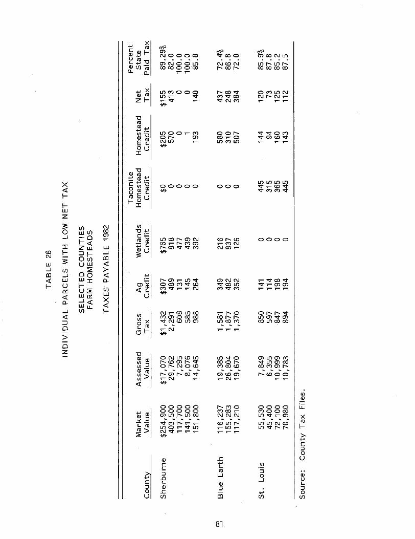
TA

BL

E

26

IND

IVID

UA

L

PAR

CE

LS

WIT

H

LOW

N

ET

TA

X

SEL

EC

TE

D

CO

UN

TI

ES

FAR

M

HO

ME

STE

AD

S

TA

XE

S PA

YA

BL

E

1982

Tac

onit

e P

erce

nt

Mar

ket

Ass

esse

d G

ross

A

g W

etla

nds

Hom

este

ad

Hom

este

ad

Net

S

tate

C

ount

y V

alue

V

alue

T

ax

Cre

dit

C

red

it

Cre

dit

C

red

it

Tax

Pa

id

Tax

Sh

erb

urn

e $2

54,9

00

$17,

070

$1,4

32

$307

$7

65

$0

$205

$1

55

89.2

9%

403,

500

29,7

62

2,29

1 48

9 81

8 0

570

413

82.0

11

7,70

0 7,

295

608

131

477

0 0

0 10

0.0

141,

500

8,07

6 58

5 14

5 43

9 0

1 0

100.

0 15

1,80

0 14

,645

98

8 26

4 39

2 0

193

140

85.8

00

B

lue

Ear

th

116,

237

19,3

85

1,58

1 34

9 21

6 0

580

437

72.4

%

---'

155,

283

26,8

04

1,87

7 48

2 83

7 0

310

248

86.8

11

7,21

0 19

,670

1,

370

352

126

0 50

7 38

4 72

.0

St.

L

ouis

55

,530

7,

849

850

141

0 44

5 14

4 12

0 85

.9%

45

,400

6,

355

597

114

0 31

5 94

73

87

.8

72,1

00

10,9

99

847

198

0 36

5 16

0 12

5 8

5.2

70

,980

10

,783

89

4 19

4 0

445

143

112

87.5

So

urc

e:

Cou

nty

Tax

F

iles

.

D. CIRCUIT BREAKER

The circuit breaker is, after the homestead credit, Minne­sota's second largest direct property tax relief program. In 1981, homeowners received $54.1 million and renters received $114.2 million from the state under this program. In 1984, according to Minnesota Department of Revenue projections, homeowners will receive $76 million and renters will receive $143 million. Benefits through the program are based on the amount of property taxes or rent paid in relation to household income. Homeowners are eligible for this pro­gram when their property taxes exceed a certain percentage of house­hold income. This percentage ranges from 0.5 percent for incomes less than $3,000 to 4.0 percent for incomes over $100,000. Renters become eligible in the same way except that they count 23 percent of rent (excluding utilities) as property taxes.

Income-related property tax relief programs are commonly divided into two types--the threshold type and the sliding scale type. Under the threshold type formula, the credit equals property taxes in excess of a certain percentage of income up to a maximum credit amount. Under the sliding scale type formula, the credit equals a percentage of tax where the percentage declines as income increases. Minnesota's circuit breaker is a threshold type formula under which a household becomes eligible when property taxes after the homestead credit exceed a certain percentage of income. To determine the amount of circuit breaker credit, one first calculates a total credit based on gross property taxes and income, and then subtracts the homestead credit from the total credit to obtain the circuit breaker credit. If the homestead credit equals or exceeds the total credit calculated under the circuit breaker formula, the homeowner is not eligible for the circuit breaker.

The circuit breaker currently has an income limit of $33,000 for homeowners who are under 65 and not disabled because their homestead credit always equals or exceeds the total credit allowable under the circuit breaker formula. There is no income limit for senior citizens or disabled persons because their circuit breaker maximum is higher than the homestead credit maximum at all income levels.

Table 27 summarizes the threshold percentages and maximum credits by income level for the current circuit breaker. The maxi­mums for senior citizens and the disabled are up to $200 higher than they are for other households.

82

TABLE 27

THRESHOLD PERCENTAGES AND MAXIMUM CREDIT AMOUNTS UNDER MINNESOTA'S CIRCUIT BREAKER

Under Age 65 Senior Citizen Threshold and Non-Disabled or Disabled

Percent First Overall First Overall Household Income of Income Maximum Maximum Maximum Maximum Gross

Loss - $ 0 09: • 0 $650 $1,000 $850 $1,000 $ 1 - 2,999 .5 650 1,000 850 1,000

3,000 - 3,999 .6 650 1,000 850 1,000 4,000 - 4,999 .7 650 1,000 850 1,000 5,000 - 5,999 .8 650 1,000 850 1,000 6,000 - 6,999 .9 650 1,000 850 1,000

7,000 - 7,999 1.0 650 1,000 850 1,000 8,000 - 8,999 1.1 650 1,000 850 1,000 9,000 - 9,999 1.2 650 1,000 850 1,000

10,000 - 10,999 1.3 650 1,000 850 1,000 11,000 - 11,999 1.4 65a 1,000 850 1,000

12,000 - 19,999 1.5 650 1,000 850 1,000 20,000 - 20,999 1.6 650 1,000 850 1,000 21,000 - 21,999' 1.6 633 975 833 992 22,000 - 22,999 1.6 617 950 817 983

23,000 - 23,999 1.8 600 925 800 975 24,000 - 24,999 1.8 583 900 783 967 25,000 - 25,999 1.8 567 875 767 958 26,000 - 26,999 2.0 550 850 750 950 27,000 - 27,999 2.0 545 820 745 930

28,000 - 28,999 2.0 540 790 740 910 29,000 - 29,999 2.0 535 760 735 890 30,000 - 30,999 2.0 530 730 730 870 31,000 - 31,999 2.2 525 700 725 850 32,000 - 32,999 2.2 520 670 720 830

33,000 - 33,999 2.2 515 640 715 810 34,000 - 34,999 2.2 510 610 710 790 35,000 - 35,999 2.2 505 580 705 770 36,000 - 40,999 2.4 500 550 700 750 41,000 - 44,999 2.6 500 550 700 750

45,000 - 52,999 2.8 500 550 700 750 53,000 - 65,999 3.0 500 550 700 750 66,000 - 81,999 3.2 500 550 700 750 82,000 - 99,999 3.5 500 550 700 750

100,000 - and Over 4.0 500 550 700 750

Source: Minnesota Department of Revenue.

83

To illustrate how the circuit breaker works, consider a homeowner under 65 who is not disabled and whose household income is $15,000. The threshold equals 1.5 percent of $15,000, or $225. If this homeowner1s gross tax were $500, the total credit would be $275 [the difference between the gross tax ($500) and the threshold ($225)]. However, since $275 is less than the homestead credit of $290 (58 percent of $500), this homeowner would not receive a refund through the circuit breaker. Now, if the gross tax were $875 instead of $500, the total credit would be $650 ($875 minus $225). Since the homestead credit would be $508 (58 percent of $875), the circuit breaker credit would be $142 (the difference between the oVer-ail credit and the homestead credit). Note that the total credit equals the first maximum of $650 shown in Table 27. As long as the total credit does not exceed the first maximum, it increases dollar for dollar with increases in the g ross property tax. However, after the total credit reaches the first maximum, the total credit rises one dollar for every two dollar increase in gross property taxes until the total credit equals the over-all maximum. For example, if the gross property tax were $1,075, the difference between gross property taxes and the threshold would be $850 ($1,075 - $225). Since $850 is more than $650, the total credit would be $650 plus one-half of the remaining $200 ($850 - $650), or a total of $750.

1. COST HISTORY

Minnesota has had income-related property tax relief pro­grams since 1968, but they became a major cost after the current circuit breaker began in 1976. Table 28 shows that the circuit breaker1s cost has exceeded $120 million every year since 1976 and is projected to reach $200 million per year in 1983. Prior to 1976, the total annual cost of the two programs replaced by the circuit breaker never exceeded $35 million. One of the programs replaced by the circuit breaker provided property tax relief for senior citizens and the disabled based on income and taxes (or imputed taxes in the case of renters). The second program was a rent credit program for all ages but was not based on income. Costs increased in 1976 because the circuit breaker expanded coverage to homeowners under 65 and increased benefit levels for both homeowners and renters.

The total cost of the circuit breaker grew from $121.7 mil.lion in 1976 to $195.2 million in 1978 and then declined to $168.3 million in 1981. The cost increased in 1978 because of higher benefits and declined in the following three years because of large increases in the homestead credit. Circuit breaker benefits for homeowners decline when homestead credit increases because there is often a dollar for dollar substitution effect between these two programs. As a result, the benefits for homeowners fell from $123.4 million in 1978 to $54.1 million in 1981. During this same time period, the benefits for renters grew from $71.8 million in 1978 to $114.2 million in 1981 because of increases in both number of applicants and credit amounts.

84

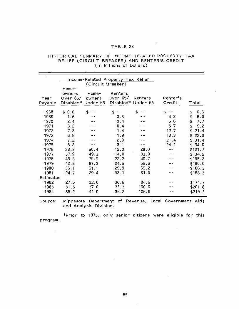
TABLE 28

HISTORICAL SUMMARY OF INCOME-RELATED PROPERTY TAX RELIEF (CIRCUIT BREAKER) AND RENTER1S CREDIT

Year Payable

1968 1969 1970 1971 1972 1973 1974 1975 1976 1977 1978 1979 1980 1981

Estimated 1982 1983 1984

(I n Millions of Dollars)

I ncome- Related Pro~ert1: Tax Relief (Circuit Breaker)

Home-owners Home- Renters

Over 65/ owners Over 65/ Renters Disabled* Under 65 Disabled* Under 65

$ 0.6 $ $ $ 1.6 0.3 2.4 0.4 3.2 0.4 7.3 1.4 6.8 1.9 7.2 2.9 6.8 3.1

33.2 50.4 12.0 26.0 37.9 49.3 14.0 33.0 43.8 79.5 22.2 49.7 42.6 67.3 24.5 55.6 36.1 51.1 29.9 69.2 24.7 29.4 33.1 81.0

27.5 32.0 30.6 84.6 31.5 37.0 33.3 100.0 35.2 41.0 36.2 106.9

Renter1s Credit Total

$ $ 0.6 4.2 $ 6.0 5.0 $ 7.7 5.7 $ 9.2

12.7 $ 21.4 13.3 $ 22.0 21.4 $ 31.4 24.1 $ 34.0

$121.7 $134.2 $195.2 $190.0 $186.3 $168.3

$174.7 $201.8 $219.3

Source: Minnesota Department of Revenue, Local Government Aids and Analysis Division.

*Prior to 1973, only senior citizens were eligible for this program.

85

Estimates for 1982 and projections for 1983 and 1984 indicate that the cost of the circuit breaker program will reverse its recent downward trend and will grow from $168.3 million in 1981 to $219.3 million in 1984. This shift will occur because property taxes rose significantly in 1982 and are expected to continue rising in the future. Further, these projections assume that there will be no change in the homestead credit or circuit breaker programs. If the homestead credit were reduced, cost estimates for the circuit breaker would be higher.

2. PURPOSES OF THE CIRCUIT BREAKER

Three major purposes have shaped Minnesota's circuit breaker. These are:

• to make the property tax more progressive;

.• to relieve high tax burdens relative to income for low and middle income households; and

• to compensate renters for tax breaks already received by homeowners through the homestead credit and income tax.

These objectives are generally consistent with each other but the circuit breaker could be designed to accomplish more of one objective at the expense of another. For example, relieving excessive tax burdens relative to income and giving more aid to renters both make the tax system more progressive. But giving less aid to renters and more aid to middle income homeowners with high taxes may be consistent with the second objective but inconsistent with the first and third objectives.

As we will show in Chapter I V, the circuit breaker effec­tiv.ely makes the tax system more progressive and provides aid to renters. In this section, we focus on how well the circuit breaker accomplishes the second objective, that of relieving excess property tax burdens for low and middle income households.

For all income levels over $3,000, the average statewide property tax. isn't very high, amounting to less than 2.5 percent of household income. However, there is great variation in property taxes for individual homeowners at any particular income level. Property taxes vary because of differences in house value and loca­tion. I n turn, house value varies because of differences in wealth, family size, and housing preferences as well as income. An underly­ing principle behind the circuit breaker is that at any income level, the credit should increase as property taxes increase and at any tax level, the credit should increase as income declines. We have analyzed how well the circuit breaker targets aid to those with high tax burdens in relation to income.

We found that the circuit breaker is becoming less effective because more homeowners are reaching the income limits and the maximum credit. While family incomes have increased rapidly since

86

the circuit breaker began in 1976, the circuit breaker1s income limit for homeowners under 65 has declined from $36,000 to $33,000 because of increases in the homestead credit. Changes in the homestead credit affect who is eligible for· the circuit breaker because if the homestead credit exceeds the total credit calculated under the circuit breaker formula, the homeowner is ineligible for the circuit breaker. In 1976, only high income families were over the income limit but now the median family income in the Twin Cities metropolitan area is coming close to the $33,000 income limit. As a result, many middle income homeowners will no longer receive circuit breaker refunds regardless of how high their property taxes become.

Similarly, while gross property taxes have been increasing, the circuit breaker1s maximum credit has not changed since 1980. Consequently, as can be seen from Table 29, the number of home­owners at the maximum has grown rapidly from 1978 to 1982 and will continue to grow in the future under the current circuit breaker program. I n the Twin Cities metropolitan area, nearly half of home­owners with incomes less than $33,000 will be at the circuit breaker maximum by 1984.

TABLE 29

HOMEOWNERS AT THE CIRCUIT BREAKER MAXIMUM IN 1978,1982, AND 1984

Among Homeowners with Incomes Under $33,000*

Number of Homeowners at the Maximum

1978* 1982 1984

7 Metro Counties 38,710 75,840 109,840

80 Outstate Counties

State Total

10,990

49,700

25,410 44,100

101,250 153,940

Percent of Homeowners at the Maximum

1978* 1982 1984

9% 27% 47%

**

**

Source: Office of Legislative Auditor analysis of Minnesota Depart­ment of Revenue1s computer file of circuit breaker returns filed in 1978.

*For 1978, includes homeowners with incomes under $36,000, which was the circuit breaker1s income limit for homeowners under 65. Now, the income limit is $33,000.

**Breakdown of homeowners by income not yet available for non­metropol itan counties. Data for the seven county metropolitan area was obtained from the 1978 Annual Housing Survey.

87

This means that in the Twin Cities metropolitan area, the circuit breaker will soon give the same credit to homeowners who have high property taxes as it does to homeowners at the same income level who have average property taxes.

Another problem that occurs when many homeowners reach the maximum credit is that many homeowners with the same property tax will receive the same credit regardless of whether their income is $20,000 or less than $5,000. All senior citizen and disabled home­owners with incomes less than $20,000 will receive the maximum credit of $1,000 if their gross property taxes exceed $1,450. The same situation exists for homeowners under 65 if their gross taxes exceed $1,650. By 1984, many senior citizens in the Twin Cities metropolitan area will be in this situation. If gross property taxes increase by 25 percent between 1982 and 1984, all senior citizens and disabled per­sons who have incomes less than $20,000 and who own homes in Minneapolis or St. Paul worth more than $68,000 in 1982 will receive the same maximum credit.

These situations lead to the question: at what tax level should homeowners reach the circuit breaker's maximum credit? In the past, the level was well above the average tax in the Twin Cities metropolitan area. Soon it will be at the average tax level, and homeowners will bear the full burden of any tax above that average. Critics of the circuit breaker may argue that this is desirable because those with higher taxes tend to have more wealth and/or receive more services and thus do not deserve more credit.

Supporters of the circuit breaker may argue that high taxes may reflect larger families, preferences for housing instead of other goods, or inequities in assessment practices and community tax rates. As a result, they would argue that homeowners with high taxes deserve more credit than homeowners with average taxes.

To determine whether the circuit breaker should target more credit to homeowners with high taxes, one must answer ques­tions such as: how much higher should taxes be on a $95,000 house compared to a $75,000 house when each homeowner has the same income? Table 30 shows how property tax burden varies with income and house value in four cities in Hennepin county for property taxes payable in 1982 and projected taxes payable in 1984. The four cities include two with tax rates higher than the metropolitan average (Robbinsdale and Minneapolis), one with a tax rate near the median for the metropolitrn area (Bloomington), and one with a below average tax rate (Edina).

IThese rankings are based on Citizens League estimates of 1982 property taxes paid on a $75,000 house in 96 metropolitan com­munities. See CL News, (Minneapolis, MN: Citizens League), March 30, 1982.

88

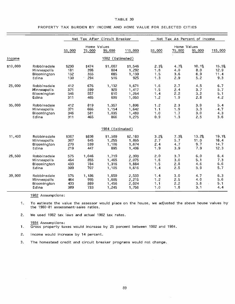
TABLE 30

PROPERTY TAX BURDEN BY INCOME AND HOME VALUE FOR SELECTED CITIES

Net Tax After Circuit Breaker Net Tax As Percent of Income

Home Values Home Values 55,000 75 1000 95 1000 115 1000 55 1000 75 1000 95 1000 115 1000

Income 1982 (Estimated)

$10,000 Robbinsdale $230 $474 $1,007 $1,546 2.3% 4.7% 10.1% 15.5% Minneapolis 1'81 398 804 1,292 1.8 4.0 8.0 12.9 Bloomington 152 355 685 1,139 1.5 3.6 6.9 11.4 Edina 130 294 516 925 1.3 2.9 5.2 9.3

25,000 Robbinsdale 412 676 1,132 1,671 1.6 2.7 4.5 6.7 Minneapolis 371 599 929 1,417 1.5 2.4 3.7 5.7 Bloomington 346 557 810 1,264 1.4 2.2 3.2 5.1 Edina 311 465 699 1,050 1.2 1.9 2.8 4.2

35,000 Robbinsdale 412 819 1,357 1,896 1.2 2.3 3.9 5.4 Minneapolis 371 666 1,154 1,642 1.1 1.9 3.3 4.7 Bloomington 346 581 1,035 1,489 1.0 1.7 3.0 4.3 Edina 311 465 866 1,275 0.9 1.3 2.5 3.6

1984 (Estimated)

11,400 Robbinsdale $367 $836 $1,509 $2,183 3.2% 7.3% 13.2% 19.1% Minneapolis 307 645 1,255 1,865 2.7 5.7 11.0 16.4 Bloomington 270 539 1,106 1,674 2.4 4.7 9.7 14.7 Edina 219 447 895 1,406 1.9 3.9 7.9 12.3

28,500 Robbinsdale 575 1,046 1,719 2,393 2.0 3.7 6.0 8.4 Minneapolis 464 855 1,465 2,075 1.6 3.0 5.1 7.3 Bloomington 433 784 1,316 1,884 1.5 2.8 4.6 6.6 Edina 389 707 1,105 1,616 1.4 2.5 3.9 5.7

39,900 Robbinsdale 575 1,186 1,859 2,533 1.4 3.0 4.7 6.3 Minneapolis 464 995 1,605 2,215 1.2 2.5 4.0 5.6 Bloomington 433 889 1,456 2,024 1.1 2.2 3.6 5.1 Edina 389 733 1,245 1,756 1.0 1.8 3.1 4.4

1982 Assumptions:

1. To estimate the value the assessor would place on the house, we adjusted the above house values by the 1980-81 assessment-sales ratios.

2. We used 1982 tax laws and actual 1982 tax rates.

1984 Assumptions: 1. Gross property taxes would increase by 25 percent between 1982 and 1984.

2. Income would increase by 14 percent.

3. The homestead credit and circuit breaker programs would not change.

89

At each income level and in all four metropolitan cities, homeowners pay at least 50 percent more property taxes on a $75,000 home than they pay on a $55,000 home and they pay at least 50 percent more taxes on a $95,000 home than they pay on a $75,000 home. Taxes rise rapidly as home values increase for three reasons. First, under Minnesota's classification structure, the portion of a home's estimated market value above $54,000 is taxed at a substantially higher rate than the initial $54,000. Second, houses in the metropoli­tan area generally reach the maximum homestead credit at values between $55,000 and $75,000. Finally, houses in the Twin Cities metropolitan area often reach the first circuit breaker maximum when their value is near $55,000 and reach the over-all maximum between $75,000 and $95,000.

Further, under current property tax relief programs, these differences will become larger in the future. For example, in 1982, Minneapolis homeowners who are under 65 and earn $25,000 pay a tax of $599 on a $75,000 home and $929 on a $95,000 home, a difference of $330, or 55 percent. Thus, the difference in taxes between these two homes is already large, and will become larger as taxes increase, because the $75,000 home is not at the maximum in 1982 but the $95,000 home is at the maximum circuit breaker credit. If gross property taxes increase by 25 percent and income increases by 14 percent, the taxes on the $75,000 home will grow by 43 percent compared to 58 percent on the $95,000 home. As a result, the home­owner wou I d pay a tax of $855 on the $75,000 hou se and $1,465 on the $95,000 house, a difference of $610, or 71 percent.

3. CRITICISMS OF THE CIRCUIT BREAKER

I n the previous section we concluded that the circuit breaker successfully achieves most of its ob}ectives. Although it is becoming less effective at relieving high tax burdens, this problem can be avoided by adjusting the circuit breaker's design. Even though the circuit breaker may meet its objectives, critics claim that it creates undesirable side effects and new inequities. Steven Gold, economist for the National Conference of State Legislatures, summarizes criti:; cisms of the circuit breaker in his book, Property Tax Relief. These criticisms include the following:

• The circuit breaker creates an incentive for some local governments to spend excessively.

• At any income level, the circuit breaker gives the most credit to homeowners with the greatest property wealth.

• I n some situations, the circuit breaker is inconsistent with the principle that taxes should be related to benefits re­ceived.

ISteven D. Gold, Property Tax Relief (Lexington, Mass.: D.C. Heath and Company, 1979), pp. 55-72.

90

• A rebate system should not be based on a single housing expense such as the property tax when there are other more significant housing expenditures which could be in­cluded.

• The circuit breaker should not give more credit to senior citizens than it gives to other homeowners with the same income and taxes.

I n this section, we review these criticisms in light of Minne­sota1s current circuit breaker. I n the following section, we examine policy alternatives, such as the sliding-scale formula, which reduce the magnitude of some of these problems.

One criticism of property tax relief in general and the cir­cuit breaker in particular is that it makes local governments less accountable for their spending decisions and thus may lead to exces­sive spending. Under the current circuit breaker, when property taxes exceed a certain percentage of household income, the circuit breaker will fully reimburse the homeowner for future tax increases up to a maximum credit. For example, a homeowner wjth an income of $10,000 pays a tax of $130 if the g ross tax is between $310 and $780 (between $310 and $980 for elderly and disabled homeowners). Thus, local governments could enact large tax increases without affecting some homeowners.

There is some evidence, though not conclusive, that the circuit brearer in Michigan may have affected electibns on local spend­ing issues. This may be an important consideration if many areas in Minnesota have a large percentage of homeowners who would be fully reimbursed for future tax increases. I n order to estimate how many homeowners would be fully reimbursed for tax increases, we analyzed a 10 percent sample of circuit breaker returns.

We estimate that in 1982, the circuit breaker reimburses 100 percent of a property tax increase for 8 percent of homeowners in the Twin Cities metropolitan area and for 18 percent of outstate home­owners. The amount by which the gross property tax could be increased without affecting the tax actually paid by these homeowners varies from $1 to nearly $850, depending on how close they are to the maximum credit.

We also estimated the number of homeowners who would be fully reimbursed for property tax increases in 1978 and 1984. As shown in Table 31, this number has declined since 1978 and will con­tinue to decline in the future if no changes are made in the circuit breaker and homestead credit. This decline has occurred because fewer homeowners are eligible now than in the past and because more homeowners reach the maximum when gross property taxes increase. But if the homestead credit were substantially reduced, more home­owners would be eligible for the circuit breaker and the number of homeowners who would be fully reimbursed for a property tax il)crease could rise substantially.

1 Gold, Property Tax Relief, p. 65.

91

TABLE 31

HOMEOWNERS FULLY REIMBURSED BY THE CIRCUIT BREAKER FOR A PROPERTY TAX INCREASE

Number of Percent Homeowners Number of Homeowners of Homeowners

(1978) Fulli: Reimbursed Fulli: Reimbursed 1978 1982 1984 1978 1982 1984

7 Metro Counties 433,000 71,000 33,000 18,000 16% 8% 4%

80 Outstate Counties 566,000 153,000 103,000 84,000 27 18 15

State Total 999,000 224,000 136,000 102,000 22% 14% 10%

Source: Office of Legislative Auditor analysis of Minnesota Depart­ment of Revenue's computer file of circuit breaker returns filed in 1978.

Henry Aaron, economist at the Brookings Institution, criti­cizes the circuit breaker because at any income 11evel, homeowners with the greatest wealth receive the most credit. This occurs be­cause homeowners with the most wealth tend to have more expensive homes and pay higher taxes and because the circuit breaker increases credit as taxes rise. This is a weakness of the circuit breaker as well as other property tax relief programs which relate credits to taxes. This argument especially applies to situations where the circuit breaker refunds all taxes in excess of a certain percentage of income. For homeowners in this situation, differences in wealth have no affect on property taxes. One can also argue that the circuit breaker is inequitable when taxes are not related to services received. Persons who have the same income and who own homes of the same value can pay the same taxes because of the circuit breaker even if their communities provide different levels of services.

The Advisory Commission on I ntergovernmental Relations argues that 100 percent of property tax increases should be rebated because it removes inequities in the property tax az--ising from fiscal tax disparities and from faulty assessment practices. However, many analysts counter that aid to local governments is the best way to deal

1 Henry Aaron, Who Pai:s the Properti: Tax? A New View. (Washington, D.C.: The Brookings Institutition, 1975).

2Advisory Commission on I ntergovernmental Relations, Properti: Tax Circuit Breakers: Current Status and Polici: Issues (Washington, D.C.: 1975), p. 10.

92

with these property tax inequities. 1 This approach not only avoids undesirable side effects but also is more comprehensive since it covers property taxes on all types of property. The problem with direct property tax relief programs is that they cannot easily separate the desirable effects of the property tax from the undesirable effects. For example, including net worth in the circuit breaker1s credit formula may be impractical because net worth is difficult to measure and verify.

These conflicting objectives lead to the question: How should the circuit breaker balance these desirable and undesirable effects of the property tax? While this is a difficult question to answer, there appears to be little reason for the credit rate structure of Minnesota1s circuit breaker. The term IIcredit rate ll refers to the proportion of a tax increase rebated by the circuit breaker to the homeowner. Under Minnesota1s circuit breaker, the credit rate equals 100 percent prior to the first maximum, 50 percent between the first and second maximum, and 0 percent thereafter. Nearly two-thirds of homeowners who are eligible for the circuit breaker are either at one extreme of 100 percent or the other extreme of 0 percent. Reducing the number of homeowners at these extremes would make the circuit breaker more equitable.

Aaron also criticizes the circuit breaker because there is no compelling reason to bUildz a rebate system around a single expense such as the property tax. The property tax is one of many housing expenses which may be a heavy burden for a family1s income. Many homeowners may have high housing expenses because of high interest rates and home prices even if their property taxes are low. Other homeowners who bought their home when interest rates and housing prices were low may have low total housing expenses even though their property taxes are high.

Yet, for families with the same income, the circuit breaker will give more credit to homeowners with high property taxes and low total housing expenses than to homeowners with low property taxes and high total housing expenses.

Another criticism of the circuit breaker is that it gives more credit to the elderly than to other homeowners with the same taxes and incomes. Under Minnesota1s circuit breaker, the maximum credit for the elderly is up to $200 higher than it is for the non­elderly. The difference in the over-all maximum becomes smaller for low income households.

The property tax can be especially burdensome for the elderly because they tend to have high taxes and low incomes. But under programs which take income and tax load into account, the

1Gold , Property Tax Relief, p. 64 and, George E. Peterson, Ed., Property Tax Reform (Washington, D.C.: The Urban Institute, 1973), and, Citizen1s League, Reducing Property Tax Ineguities Among Taxpayers and Cities, 1975.

2 Aaron, Who Pays the Property Tax? A New View.

93

issue is not whether the elderly deserve tax relief, but whether the elderly deserve special treatment beyond what their income and tax situations would lead to. A burden peculiar to the elderly is the sudden drop in income that many experience at retirement. Since property taxes tend to keep rising, the elderly face either a difficult cash flow problem if they remain in their homes or the stress that can occur if they must give up their homes. These problems, however, should be weighed against the financial advantages which the elderly enjoy over the non-elderly at the same income level. Special programs for the elderly include Medicare and a double exemption on the income tax. Furthermore, the elderly tend to have fewer dependents and higher net worth than do younger families. The arguments in favor of special treatment of the elderly apply primarily to low income elderly homeowners. As a result, there appears to be no justification for giving middle and high income elderly significantly higher maxi­mums.

4. POLICY ALTERNATIVES

Many of the problems with the circuit breaker can be elimi­nated or reduced by changing the design of the circuit breaker. Alternatives listed below are divided into those that raise costs and those that reduce costs. These alternatives keep 'the current thresh­old approach of the circuit breaker. Another alternative is to change the threshold formula to a sliding scale formula. This alternative could cost more or less than the current circuit breaker, depending on the specific design chosen.

Options which increase costs:

• Raise the circuit breaker's maximum credit amounts.

• I ncrease the circuit breaker's income brackets.

Options which reduce costs:

• Reduce the circuit breaker's 100 percent credit rate.

Options which can either increase or decrease cost:

• Change to a sliding scale formula.

The options which increase the maximum credit and/or reduce credit rates will reduce the number of homeowners who are at the circuit breaker maximum credit and thus more effectively target property tax relief to homeowners with high taxes relative to income. In addition, raising the maximum can increase the income limit for homeowners who are under 65 by setting the circuit breaker's over-all maximum higher than the homestead credit maximum. Currently, homeowners who are under 65 and earn more than $33,000 are not eligible because the homestead credit maximum is higher than the circuit breaker maximum in this income range.

94

I ncreasing income brackets can ensure that middle income homeowners do not become ineligible simply because their incomes have increased with inflation, This will help maintain tax differences between middle and high income homeowners. However, by itself, it will not help resolve the problems caused by too many people reaching the maximum.

While all three of these options can improve the circuit breaker, reducing the circuit breaker's 100 percent credit rate has several advantages over the other two. First, it reduces costs whereas the other two options increase costs. These cost savings can be used to also raise the maximums and/or to increase the income brackets.

I n addition, reducing the 100 percent credit rate ensures that homeowners pay at least a part of any property tax increase and thus may reduce the incentive for local governments to spend exces­sively. Because of this change, the circuit breaker would also more uniformly relate property taxes to wealth and level of local services. These improvements would be especially important if the Legislature substantially lowered either the homestead credit's $650 maximum or its 58 percent credit rate because many homeowners would become eligible for the circuit breaker and would receive 100 percent rebates on future property tax increases.

One possible disadvantage of reducing the credit rate is that some homeowners will lose benefits. At a time when property taxes are rising rapidly, this may appear to place an unacceptable burden on these taxpayers. However, the homeowners who would lose the most benefits from this change are those for whom the circuit breaker now rebates 100 percent of a property tax increase. By reducing benefits for these homeowners and ralsmg benefits for homeowners at the maximum, tax increases can be distributed more evenly than they would be under the current circuit breaker.

We conclude that adopting all three of the above options will improve the effectiveness of the circuit breaker without necessarily increasing costs. If funds are not sufficient to maintain the current circuit breaker program, reducing the 100 percent credit rate appears to be the most effective alternative. Another option which can have similar advantages as the options discussed above is the sliding scale formula. Since this formula replaces the 100 percent credit rate with variable rates depending on income, it avoids problems caused by the 100 percent credit rate. How well it targets property tax relief to homeowners with high taxes depends on its specific maximums, credit rates, and income limits.

A criticism of the sliding scale circuit breaker is that it gives more credit to homeowners with low taxes and thus either is more expensive than the threshold ap~roach or gives less credit to homeowners with high property taxes. I n Minnesota, this criticism is not as valid as it is in other states because Minnesota also has a

1 Gold, Property Tax Relief, pp. 64-65.

95

homestead credit which gives credit to homeowners with low taxes. I n fact, if the homestead credit and circuit breaker were replaced by a comprehensive sliding scale credit program, less credit would go to high income homeowners with low taxes and more funds would be available for homeowners with high taxes. Further, such a sliding scale program would maintain the relation between income and credit for homeowners with low taxes as well as for homeowners with high taxes. Under the current circuit breaker and homestead credit, many homeowners are not eligible for the circuit breaker because their taxes are not high enough, and thus they receive a credit equal to 58 percent of gross property taxes regardless of income.

E. ADMINISTRATION OF THE CIRCUIT BREAKER FOR RENTERS (THE RENTER1S CREDIT)

A major problem with the circuit breaker program for renters is that the information requested to determine the tax refund is subject to easy manipulation. This is especially true for information documenting the rental contract between the claimant and the landlord. The auditability of this information is also seriously restricted because of limited accessability to non-taxable income data and cost inefficien­cies associated with verifying rent paid.

I n order to qualify for a renter1s property tax refund, claimants must have been full or part-year residents of Minnesota during the respective tax year and must have leased or rented the unit in which they resided during that year. The unit in which the claimants ··Iived must also have been subject to property taxes or payments lIin lieu ll of property taxes.

If a rental unit is occupied by two qualified married indi­viduals, only one claim per household is allowed. If the unit is rented by two or more unrelated individuals, then each must file a separate claim with the rent divided equally between them. Their individual household incomes are then used to determine individual refund amounts.

To receive a renter1s property tax refund, a claimant completes a Minnesota property tax refund return (M-1 PR) providing total household income and rent paid for the given tax year. The claimant must also attach a certificate of rent paid (CRP) which is intended to document both the total rent for occupancy and other relevant information such as the number of occupants living in the unit, whether utilities are included in the rent, the rental period, and whether property taxes were paid. Given the nature of the information requested and the system by which it is reported, serious problems are presented which restrict and often prohibit effective auditability of individual claims.

I n providing total household income, claimants are required to report not only their federal adjusted gross income but also non­taxable income from such sources as social security, unemployment

96

and workers ' compensation and public assistance. 1 The major problem is that documentation of non-taxable income is not required, nor is it readily available from either the recipient or from the provider. Thus, unlike reporting income for income tax purposes which is verified by such documents as W-2 forms provided by both the tax­payer and the respective employer, the. state is severely restricted in being able to verify the non-taxable income amounts as reported.

I n order to systematically verify household income for all claims, the state would have to conduct computer matches which would compare the claimant's reported income with records maintained by other state and federal agencies. This method, however, can be very costly and technically difficult and for some income sources such as public assistance payments and social security benefits, access to the information is either denied or severely restricted by data privacy laws. As a result, the accuracy and truthfulness of a claimant's re­ported or unreported household income is unverifiable.

Claimants are required to document their rent by submitting a certificate of rent paid (CRP), completed by their landlord(s), indicating the amount of rent they paid and the number of tenants occupying the unit. The CRP is subject to manipulation by both the renter and the landlord, the relationship between which can often be quite precarious. For example, the system is dependent upon a landlord's willingness to cooperate with the law by making CRP's readily available to all tenants and not cheat the system by providing favors to occupants.

The system also assumes that every landlord in the state maintains accurate records on all their rental units and respective tenants so that information documenting rent paid, rent value of furnishings, charges paid for utilities, charges paid for other items or services, and number of tenants per unit can be accurately pro­vided. It might be asking too much of the syste~ to assume that all landlords can accurately maintain such information.

Other than responding to demands by tenants, the system provides little incentive to the landlord to accurately and faithfully administer the CRP. Although Minnesota law requires landlords to provide a CRP to each of their renters, the penalty for not doing so amounts to only $20 for each failure to act (M.S. 290A.19). Because the penalty is so low, it is not cost effective for the state to enforce

1Total household income includes: federal adjusted gross income; workers ' compensation, unemployment compensation payments, public assistance, social security and deducted amounts for Medicare; veterans and disability payments; railroad retirement payments and all other pension and annuity payments; non-taxable interest; dividends exclusion and capital gains deductions.

2For example, it may be difficult for a landlord to keep track of the number of occupants per unit if he manages several buildings in different locations, or if the landlord manages a rather large low-income· complex where it is not uncommon to discover families doubling up in single residential units in order to reduce costs.

97

the provIsion, especially in cases involving only a few tenants per landlord. Furthermore, even if a CRP is submitted with the M-1 PR, there are no guarantees that the landlord provided the information. The fact is the CRP could easily be completed by the claimant and signed by the landlord or by a friend.

Furthermore, a claimant is even permitted to complete and file a rent paid affidavit in lieu of a CRP. Although the incidence of rent paid affidavits being filed is relatively low (approximately 1 per­cent in 1981), in such cases and to the extent the information appears to be reasonable, the state is placing full faith and trust in the claimant in providing accurate and truthful information pertaining to both rent paid and non-taxable income.

It is far more beneficial to a claimant to manipulate rent paid than to omit income. For example, a $109 addition to 'rent will change the refund bracket increasing the refund by usually $25. However, it requires a $500 omission in income to affect the refund bracket resulting in a much smaller refund differential (approximately $6 to $11).

Not only does the CRP represent an unreliable tool to document rent paid, it is virtually impossible to systematically verify the information in a cost effective manner. For example, verification of reported rent on the CRP might require a computerized match with the landlord's reported rental income on his federal or state income tax return, or it may require extensive individual audits. These methods, however, would be either technically difficult, if' not impos­sible, or hard to justify on the basis of costs and benefits. This is especially true when the average refund amount is approximately $273 per claim (tax year 1980, payable 1981). As a result, unless there are inconsistencies, omissions or exaggeration of rent, the CRP is generally accepted.

Currently, the Department of Revenue reviews all claims for property tax relief including M-1 PR refunds for renters. Reviews made during the processing phase are designed primarily to uncover internal pro,plems such as omissions, mathematical correctness, and consistency. Based upon this review, claims which have pr~blems or appear to be suspicious are selected for further scrutiny. These claimants are then usually subject to having either to respond to letters seeking clarification, or to becoming subjects of individual audits (both the renter and landlord may be audited).

1 For example: is the form signed by the claimant; is the CRP attached and completed correctly; does the information on the CRP match with what is reported on the M-1 PR, etc.

2For example: several claims having identical income and rent amounts warrant suspicion; if the claimant does not report fed­eral gross income, this may be a serious omission; and if rent seems too high relative to reported income, this may also be cause for further evaluation.

98

Prior to sending out refunds, a computer match, based on social security numbers is also performed against all other property tax relief and income tax refund claims. This is done in order to identify individuals receiving more than one refund. These claims are then more closely evaluated and reasons sought as to why multiple claims have been made.

As indicated earlier, efforts to verify information on all claims is limited. Specifically, because of data privacy laws, the Department of Revenue is not able to gain access, for purposes of verification, to information on a claimant·s reported income, or lack of income, from: welfare and Medicare; social security; workers· compen­sation; veterans and disability benefits; railroad retirement payments; and other pension and annuity payments.

However, the Department of Revenue does attempt to verify income items which appear on federally maintained data files sU!fh as federal gross income, dividends exclusions, and capital gains. In addition, since the Department of Revenue recently acquired authori­zation to access data maintained by the Department of Economic Security, it iz also developing the capacity to verify unemployment compensation.

I n effect, current review and audit efforts by the Depart­ment of Revenue is limited for two reasons; first, to conduct a more extensive systematic audit of both reported income and rent would probably not be cost effective, and second, data privacy laws and technical difficulties restrict or prohibit accessibility to most non­taxable income information. As a result, unless there were obvious problems with the completion of the forms, many types of improprieties may exist which would be very difficult to discover. For example, many types of situations, such as those listed below could exist and easily IIslipll through the current review and audit system.

• Welfare income could be excluded from household income when it should have been reported.

• Two or more unrelated individuals renting the same unit could arrange for only one person, based on a single in­come, to collect the refund--with either a rent paid affi­davit filed in lieu of a CRP or the CRP improperly adminis­tered by the landlord.

1The purpose of this match is to determine if the federal gross income reported on the M-1 PR is consistent to that reported on both state and federal income tax returns. However, this method has some limitations because there are several legitimate reasons as to why the income amounts would differ. For example, a claimant may have been only a part-y~ar resident of the state, recently married or divorced.

2 . See Minn. Stat. §268.12, Subd. 12.

99

The rental property may not have been subject to property taxes, although the CRP indicated that property taxes were paid.

• A college student under the age of 21 could be renting but claimed as a dependent by his/her parents.

• The tenant could be related to the landlord and as a result, no legitimate rent transaction actually occurred.

It could be argued that the above examples represent exceptions to the rule and may only represent a small proportion of all claims made. However, common sense would indicate that these types of situations in all Ii kelihood are not that unusual. I n fact, there is evidence to suggest that these types of problems and others may be more prevalent than previously suspected.

I n order to estimate the potential cost to the state of mis­representations made by renters on their rent credit forms, our office conducted an extensive audit on a random sample of 560 claims. Projecting the results of this sample to the population of all claims, we estimate that in 1981 the state should have paid $104.5 million in rente,l s property tax relief as opposed to the $118.7 million actually paid. This represents a potential cost of approximately $14 million attributed to claims that should have been adjusted downward or denied.

It should be emphasized, however, that the purpose of our study was only to estimate total potential costs to the state and not to demonstrate audit procedures that could be effectively used ~re­cover those costs. I n fact, based upon the audit we performed on the random sample of 560 claims, the potential audit recovery would not have been cost beneficial. We do not feel, however, that our costs can be projected to the population because of certain fixed start-up costs and the unknown factor of how efficiently the audit could be conducted if it were done on a large scale. For the Depart­ment of Revenue to recover these overpayments would require enabling legislation and an analysis of efficiency and effectiveness of a large scale recovery effort.

1The projection of our sample results indicates that there is a 95 percent probability that the true value of this number lies in the range of $104,463,378 ± $6,165,680 as opposed to the actual renter1s property tax relief paid of $118,720,265. Conversely, one can con­clude from our sample results that there is a 95 percent probability that renter1s property tax relief has been overpaid by $14,256,887 ± $6,165,680. It should also be noted that our sample was selected from calendar 1980 M1PR returns filed in 1981. We included in the population all returns where the taxpayer had checked the renter category, including renters who may also have been disabled, senior citizens or partial-year homeowners as well. The summation of renter1s property tax relief paid to this category of filers was $118,720,265.

100

Finally, it should also be noted that the Department of Revenue has uncovered a limited number of illegal or fraudulent cases. However, the emphasis is placed on prosecuting only large­scale or organized fraud. I solated incidents or claims of low value, if identified for improprieties, are usually not prosecuted. Rather, the claims are merely adjusted accordingly or denied.

101

 

IV. PROPERTY TAX AND INCOME

The property tax is often criticized because it places a dis­proportionate burden on low and moderate income persons. How a tax is distributed among different income groups is commonly described in terms of whether a tax is progressive, proportional, or regressive. A tax is progressive if high income persons pay a larger percentage of their income than low income persons pay. A tax is proportional if all income groups pay the same percentage of their income and it is regressive if high income persons pay a smaller percentage of their income than low income persons pay. One major purpose of property tax relief programs is to make the tax system more progressive by shifting taxes from the property tax to other more progressive taxes or by targeting aid directly to people with high tax burdens relative to their income. However, many economists question whether the property tax is as regressive as has been previously assumed. In this chapter, we briefly review what the literature says about who pays the property tax and examine the relationship between income and residential property taxes in Minnesota. We also examine how this relationship changes over time as property taxes increase. Finally, because property tax relief means increases in other taxes, we address how property tax relief programs affect Minnesota's tax system as a whole.

A. LITERATURE REVI EW

The traditional view that the property tax is highly regres­sive is based on the assumption that owners of businesses and apart­ments shift most of the property taxes to consumers and renters. Under this view, only the tax on land is absorbed by the owner of rental and commercial property. Homeowners pay the entire tax since they cannot shift the tax to other persons. Since consumption of housing and consumer goods make up a larger proportion of income for low income households than it does for high income households, the property tax is viewed as regressive.

During the 1970s, new studies came forth to argue that the property tax is not regressive. They conclude that property taxes reduce the rate of return on capital and as a result, most of the property tax is borne by the owners of capital. Since capital owner­ship is highly concentrated in high income households, the tax is viewed as progressive. Henry Aaron, economist at the Brookings Institution, pulled the new ,,\iew together in his book, Who Pays The Property Tax? A New View. Aaron argues that empirical studies which support the old view are biased in favor of regressive outcomes because they use annual income instead of permanent income. Aaron demonstrates that one year1s income will often be a misleading indicator

1 Henry (Washington D. C.:

Aaron, Who Pays the Property Tax? A New View. The Brookings Institution, 1975).

103

of the household's financial condition and that income over an ex­tended time period is a better predictor of consumption, particularly housing consumption. If this is the case, property taxes will be more progressive when income is measured over several years instead of one year. There is now a sizable body of literature that generally agrees that the property 1tax is not as regressive as previously thought under the old view.

Several economists do not entirely accept the new view, however, particularly the claim that tax on residential property is progressive. Netzer points out that ther~ is little empirical support for many of Aaron's theoretical arguments. For rental property, the key factors are what proportion of the property tax is shifted to renters and what is the relationship between the renter's income and taxes attributable to the renter's unit. There is a lack of reliable empirical data on both of these questions. Netzer and Peterson argue that in a highly complex property tax system, many local conditions affect whether the tax is progressive or regressive and extensive empirical analysis is req~red before one can accurately estimate who pays the property tax. As for Aaron's argument on permanent income, Netzer concedes that using permanent income may make the property tax less regressive but counters that (I) by itself, it is not significant enough to make a tax on housing consumption progressiv~ and (2) current income may be a better indicator of ability to pay.

I n summary, there is consensus in the economics literature that the property tax is not as regressive as was portrayed under the old view, but doubt remains as to whether the over-all effect is progressive or regressive. The residential portion of the property tax is generally considered to be more regressive than the business portion of the tax.

1Steven D. Gold, Property Tax Relief, (Lexington, Mass.: D. C. Heath and Company, 1979). Dick Netzer, "The I ncidence of the Property Tax Revisited," National Tax Journal, (December, 1973), pp. 515-535, Richard A. Musgrave and Peggy B. Musgrave, Public Finance in Theory and Practice, (New York: McGraw-Hili, 1976). Edgar K. Browning and Jacquelene M. Browning, Public Finance and the Price System, (New York: Macmillan Publishing Co., Inc., 1979). Harvey E. Brazer, George E. Peterson, et aI., "The Property Tax: Progressive or Regressive?", American Economic Review Papers and Proceedings, 64, (May, 1974) pp. 230-235.

2 Netzer, Ibid.

3 Netzer, Ibid; Peterson, Ibid.

4Netzer, Ibid.

104

B. INCIDENCE OF THE RESIDENTIAL PROPERTY TAX

I n this section, we examine the incidence of residential property taxes in Minnesota and how it is affected by direct property tax relief programs. I n this discussion, the incidence of a tax refers to how the tax is distributed among different income groups.

The economic literature raises numerous questions about the validity of available data on property taxes and income. As a result, it is not possible to measure accurately the incidence of the property tax as a whole. Even so, it is useful to examine data on residential property taxes and income in Minnesota because the tax on residential property is often considered to be the most regressive and objection­able part of the property tax.

To look at the relationship between income and property taxes in Minnesota, we developed a data base from Minnesota Depart­ment 9f Revenue computerized files of circuit breaker returns and income tax returns. We matched circuit breaker returns filed in 1978 with income tax returns for tax years 1975 through 1978. We used circuit breaker returns filed in 1978 because more homeowners filed in that year than any other year. I n fact, due to increases in the homestead credit and increased income in relation to property taxes, nearly twice as many homeowners filed in 1978 compared to 1981. Based on actual and projected changes in property taxes and family income, we estimated the incidence of the property tax in 1982 and 1984 under the current property tax relief programs and under some alternative progr1;lms.

This data has several advantages over other published data on income and property taxes. First, the property tax data from circuit breaker returns is documented by property tax statements sent by counties to individual homeowners, and thus is more reliable than self-reported data used by most other studies. Second, we used four years of income data (1975 through 1978) whereas most studies use only one year's income. Consequently, we could test whether the property tax on homes remains regressive when measured over several years of income.

Finally, this data enables us to estimate how Minnesota's property tax relief programs affect the incidence of the residential property tax now and in the near future. Based on actual and projected changes in property taxes and family income since 1978, we estimated the incidence of the property tax in 1982 and 1984 under the current property tax relief programs and under some alternative homestead credit programs. This can not be done with existing studies on property taxes and income. Existing studies conducted nationally or in other states are inadequate because Minnesota's prop­erty tax system differs greatly from systems in other states. The last comprehensive study on property taxes and income in Minnesota was conducted by Hatfield in 1969 and thus does not reflect the major

105

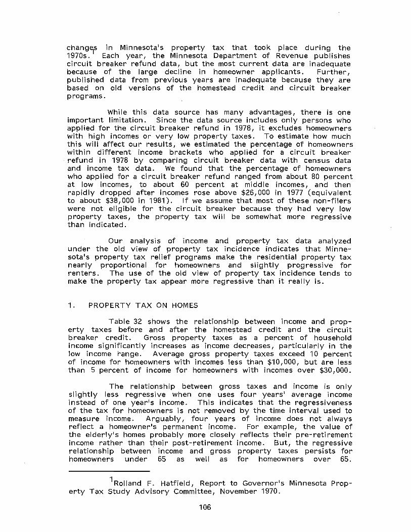
changis in Minnesota1s property tax that took place during the 1970s. Each year, the Minnesota Department of Revenue publishes circuit breaker refund data, but the most current data are inadequate because of the large decline in homeowner applicants. Further, published data from previous years are inadequate because they are based on old versions of the homestead credit and circuit breaker programs.

While this data source has many advantages, there is Qne important limitation. Since the data source includes only persons who applied for the circuit breaker refund in 1978, it excludes homeowners with high incomes or very low property taxes. To estimate how much this will affect our results, we estimated the perc~ntage of homeowners within different income brackets who applied for a circuit breaker refund in 1978 by comparing circuit breaker data with census data and income tax data. We found that the percentage of homeowners who applied for a circuit breaker refund ranged from about 80 percent at low incomes, to about 60 percent at middle incomes, and then rapidly dropped after incomes rose above $26,000 in 1977 (equivalent to about $38,000 in 1981). If we assume that most of these non-filers were not eligible for the circuit breaker because they had very low property taxes, the property tax will be somewhat more regressive than indicated.

Our analysis of income and property tax data analyzed under the old view of property tax incidence indicates that Minne­sota1s property tax relief programs make the residential property tax nearly proportional for homeowners and slightly progressive for renters. The use of the old view of property tax incidence tends to make the property tax appear more regressive than it really is.

1. PROPERTY TAX ON HOMES

Table 32 shows the relationship between income and prop­erty taxes before and after the homestead credit and the circuit breaker credit. Gross property taxes as a percent of household im:ome significantly increases as income decreases, particularly in the low income range. Average gross property taxes exceed 10 percent of income for homeowners with incomes less than $10,000, but are less than 5 percent of income for homeowners with incomes over $30,000.

The relationship between gross taxes and income is only slightly less regressive when one uses four years l average income instead of one year1s income. This indicates that the regressiveness of the tax for homeowners is not removed by the time interval used to measure income. Arguably, four years of income does not always reflect a homeowner1s permanent income. For example, the value of the elderly1s homes probably more closely reflects their pre-retirement income rather than their post-retirement income. But, the regressive relationship between income and gross property taxes persists for homeowners under 65 as well as for homeowners over 65.

1 Rolland F. Hatfield, Report to Governor1s Minnesota Prop­erty Tax Study Advisory Committee, November 1970.

106

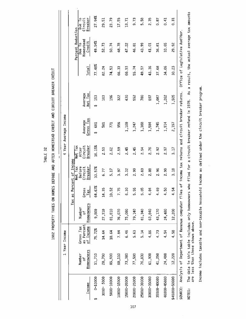
TABL

E 32

1982

PR

OPER

TY T

AXES

ON

HOM

ES B

EFOR

E AN

D AF

TER

HOM

ESTE

AD

CRED

IT A

ND

CIRC

UIT

BRE

AKER

CR

EDIT

1 Y

ear

Inco

me

4 Y

ear

Ave

rage

In

com

e

Tax

as

Per

cent

of

Inco

me

Net

Tax

N

et T

ax

Per

cent

Red

ucti

on

Num

ber

Gro

ss T

ax

Num

ber

Bef

ore

Aft

er

Due

To

Due

To

of

as P

erce

nt

of

Gro

ss

Cir

cuit

C

ircu

it

Ave

rage

A

vera

ge

Hom

este

ad

Cir

cuit

In

com

e H

omeo

wne

rs

of I

ncom

e H

omeo

wne

rs

Tax

Bre

aker

B

reak

er

Gro

ss

Tax

Net

Tax

T

otal

C

red

it

Bre

aker

$ 0-

$300

0 11

,710

75

.7'lY

o 9,

800

64.6

7%

33.5

7%

16.1

5%

$ 68

1 $

153

77.4

8%

49.5

4%

27.9

4%

3000

-50

00

28,7

00

14.6

4 27

,310

14

.35

6.77

2.

53

581

103

82.2

4 52

.73

29.5

1

5000

-100

00

85,9

30

10.6

4 81

,810

10

.52

5.17

2.

62

771

196

74.5

3 50

.74

23.7

9

1000

0-15

000

80,1

10

7.84

76

,070

7.

75

3.97

2.

59

956

322

66.3

3 48

.78

17.5

5

1500

0-20

000

73,3

80

6.46

75

,000

6.

30

3.32

2.

45

1,10

0 43

0 60

.93

47.2

2 13

.71

......

Cl

2000

0-25

000

77 ,5

00

5.63

79

,140

5.

55

2.99

2.

45

1,24

7 55

2 55

.74

46.0

1 9.

73

'-I

2500

0-30

000

I 76

,830

5.

14

81,3

40

5.05

2.

83

2.54

1,

388

700

49.5

7 43

.99

5.58

3000

0-35

000

I 61

,930

4.

86

63,8

40

4.84

2.

88

2.76

1,

584

897

43.3

6 41

.01

2.35

3500

0-40

000

41,2

90

4.73

43

,170

4.

69

2.96

2.

92

1,74

5 1,

087

37.6

8 36

.81

0.87

4000

0-45

000

i 24

,480

4.

54

24,4

80

4.50

2.

99

2.97

1,

914

1,26

2 34

.06

33.6

5 0.

41

$450

00-5

0000

_I _

12,2

20

4.58

12

,200

4.

54

3.18

3.

17

2,15

7 1,

505

30.2

3 29

.92

0.31

SOUR

CE:

Ana

lysi

s o

f D

epar

tmen

t o

f R

even

ue c

ompu

ter

file

s o

f in

com

e ta

x r

etu

rns

and

cir

cu

it b

reak

er r

etu

rns.

O

ffic

e of

Leg

isla

tiv

e A

udit

or.

NOTE

S:

The

dat

a in

th

is t

able

inc

lude

s on

ly h

omeo

wne

rs w

ho f

iled

fo

r a

cir

cu

it b

reak

er r

efun

d in

197

8.

As

a re

sult

, th

e ac

tual

av

erag

e ta

x a

mou

nts

are

less

tha

n th

ose

show

n ab

ove.

Inco

me

incl

udes

tax

able

and

no

n-ta

xabl

e ho

useh

old

inco

me

as

defi

ned

unde

r th

e cir

cu

it b

reak

er p

rogr

am.

Both the homestead credit and the circuit breaker reduce the regressiveness of the property tax on homes, making taxes nearly proportional to income over a wide income range. Net taxes are slightly regressive between $3,000 and $25,000 of income; slightly progressive between $25,000 and $40,000. If homeowners who do not apply for circuit breaker refunds because their property taxes are too low were included, we estimate that the property tax would be more regressive than shown in Table 32 but would still be nearly proportional for homeowners with incomes between $3,000 and $40,000. It is difficult to estimate tax burdens for homeowners with incomes over $40,000 because data quality rapidly declines as income rises above $40,000. Although the net tax remains substantially regressive below $3,000, less than two percent of homeowners are in this income range.

While the homestead credit distributes large amounts of credit to all income groups, it makes the property tax on homes less regressive because it reduces property taxes by a larger percentage for low-income homeowners than for high-income homeowners. This occurs because high income homeowners more often reach the maximum and thus their homestead credit equals less than 58 percent of their gross property tax.

However, the circuit breaker is the key to making the property tax nearly proportional to income. On the one hand, if the homestead credit were not supplemented by the circuit breaker, the net taxes would remain predominantly regressive, ranging from over 5 percent of income for incomes less than $10,000 to under 3 percent for incomes $20,000 and above. On the other hand, if the homestead credit were eliminated or the maximum credit reduced, the property tax would be more progressive than it is now.

2. PROPERTY TAX ON RENTAL PROPERTY

Measuring the incidence of property taxes for renters is considerably less reliable than it is for homeowners. While data on the relationship. between income and rent are reasonably accurate, measuring the tax incidence also depends on the ratio of taxes to rent and the share of taxes actually shifted to the renter. Minnesota's circuit breaker assumes that the renter pays 23 percent of the rent (excluding utilities) for property taxes. Tax-rent data representative of the entire state's rental property are not available but several studies indicate that the average ratio does not sjgnificantly exceed 23 percent in the Twin Cities metropolitan area. However, these

1The following analyses found average ratios of property taxes to rent ranging from 18.5 percent to slightly more than 23 percent in the Twin Cities metropolitan area. See Coopers and Lybrand, Analysis of Minnesota Property Taxes and the Tax Burdens on Owners of Single-Family Homes and Renters of Multi-Family Units, prepared for the Minnesota Multi-Housing Association, 1980. Minnesota Department of Revenue, Research Office, Tables on property tax/rent ratios. Urban Coalition, staff memos analyzing the Coopers and Lybrand study, December 1981.

108

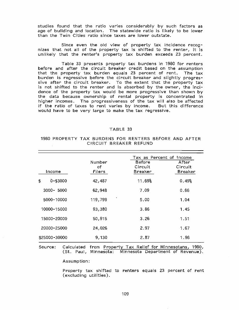
studies found that the ratio varies considerably by such factors as age of building and -location. The statewide ratio is Ii kely to be lower than the Twin Cities ratio since taxes are lower outstate.

Since even the old view of property tax incidence recog­nizes that not all of the property tax is shifted to the renter, it is unli kely that the renter's property tax burden exceeds 23 percent.

Table 33 presents property tax burdens in 1980 for renters before and after the circuit breaker credit based on the assumption that the property tax burden equals 23 percent of rent. The tax burden is regressive before the circuit breaker and slightly progres­sive after the circuit breaker. To the extent that the property tax is not shifted to the renter and is absorbed by the owner, the inci­dence of the property tax would be more progressive than shown by the data because ownership of rental property is concentrated in higher incomes. The progressiveness of the tax will also be affected if the ratio of taxes to rent varies by income. But this difference would have to be very large to make the tax regressive.

TABLE 33

1980 PROPERTY TAX BURDENS FOR RENTERS BEFORE AND AFTER CI RCU IT BREAKER REFUND

Tax as Percent of Income Number Before After

of Circuit Circuit Income Filers Breaker Breaker

$ 0-$3000 42,487 11.69% 0.49%

3000- 5000 62,948 7.09 0.66

5000-10000 119,799 5.00 1.04

10000-15000 93,380 3.86 1.45

15000-20000 50,915 3.26 1.51

20000-25000 24,026 2.97 1.67

$25000-30000 9,130 2.87 1.96

Source: Calculated from Property Tax Relief for Minnesotans, 1980, (St. Paul, Minnesota: Minnesota Department of Revenue).

Assumption:

Property tax shifted to renters equals 23 percent of rent (excluding utilities).

109

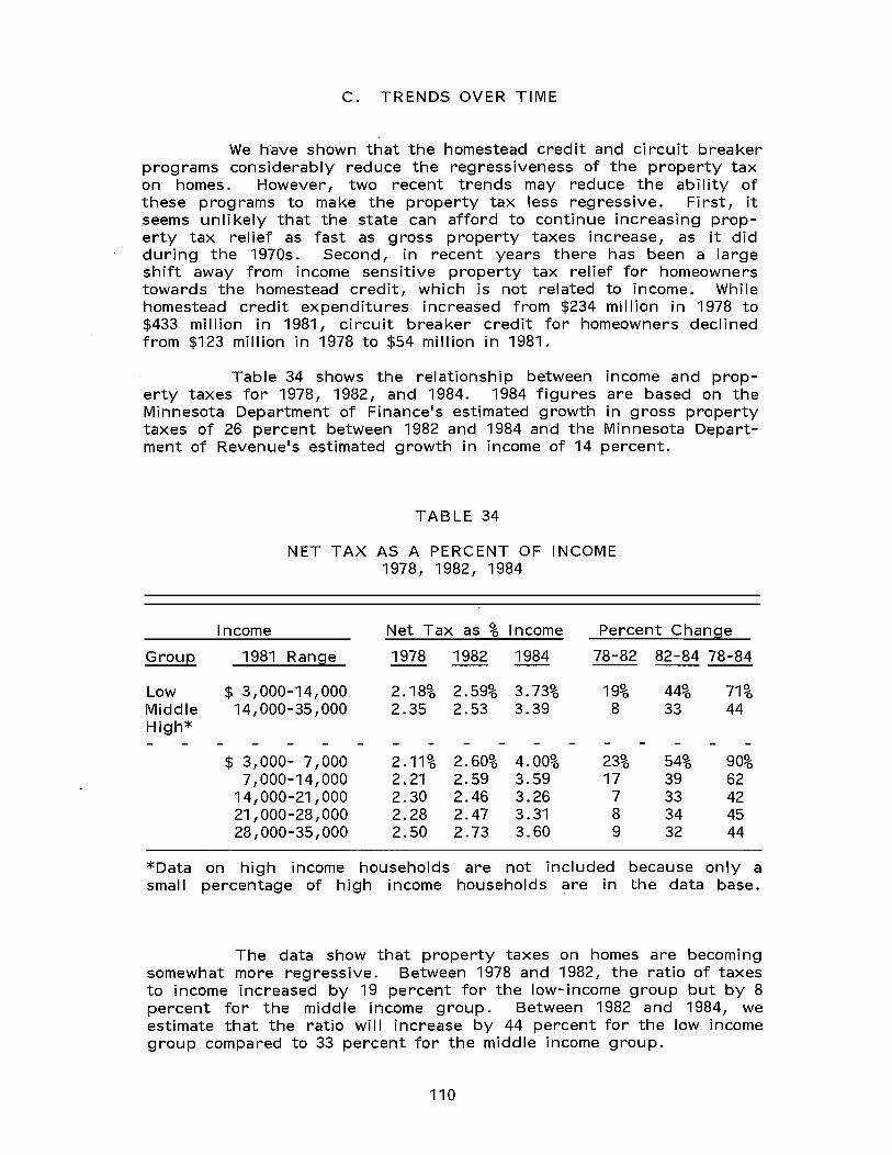
C. TRENDS OVER TIME

We have shown that the homestead credit and circuit breaker programs considerably reduce the regressiveness of the property tax on homes. However, two recent trends may reduce the ability of these programs to make the property tax less regressive. First, it seems unli kely that the state can afford to continue increasing prop­erty tax relief as fast as gross property taxes increase, as it did during the 1970s. Second, in recent years there has been a large shift away from income sensitive property tax relief for homeowners towards the homestead credit, which is not related to income. While homestead credit expenditures increased from $234 million in 1978 to $433 million in 1981, circuit breaker credit for homeowners declined from $123 million in 1978 to $54 million in 1981.

Table 34 shows the relationship between income and prop­erty taxes for 1978, 1982, and 1984. 1984 figures are based on the Minnesota Department of Finance's estimated growth in gross property taxes of 26 percent between 1982 and 1984 and the Minnesota Depart­ment of Revenue's estimated growth in income of 14 percent.

Group

Low Middle High*

*Data small

TABLE 34

NET TAX AS A PERCENT OF INCOME 1978, 1982, 1984

Income Net Tax as % Income Percent Change

1981 Range 1978 1982 1984 78-82 82-84 78-84 ----$ 3,000-14,000 2.18% 2.59% 3.73% 19% 44% 71% 14,000-35,000 2.35 2.53 3.39 8 33 44

$ 3,000- 7,000 2.11% 2.60% 4.00% 23% 54% 90% 7,000-14,000 2.21 2.59 3.59 17 39 62

14,000-21,000 2.30 2.46 3.26 7 33 42 21,000-28,000 2.28 2.47 3.31 8 34 45 28,000-35,000 2.50 2.73 3.60 9 32 44

on high income households are not included because only a percentage of high income households are in the data base.

The data show that property taxes on homes are becoming somewhat more regressive. Between 1978 and 1982, the ratio of taxes to income increased by 19 percent for the low-income group but by 8 percent for the middle income group. Between 1982 and 1984, we estimate that the ratio will increase by 44 percent for the low income group compared to 33 percent for the middle income group.

110

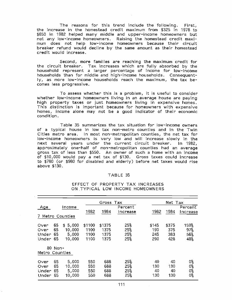
The reasons for this trend include the following. First, the increase in the homestead credit maximum from $325 in 1978 to $650 in 1982 helped many middle and upper-income homeowners but not any low-income homeowners. Raising the homestead credit maxi­mum does not help low-income homeowners because their circuit breaker refund would decline by the same amount as their homestead credit would increase.

Second, more families are reaching the maximum credit for the circuit breaker. Tax increases which are fully absorbed by the household represent a larger percentage of income for low-income households than for middle and high-income households. Consequent­Iy, as more low-income households reach the maximum, the tax be­comes less progressive.

To assess whether this is a problem, it is useful to consider whether low-income homeowners living in an average house are paying high property taxes or just homeowners living in expensive homes. This distinction is important because for homeowners with expensive homes, income alone may not be a good indicator of their economic condition.

Table 35 summarizes the tax situation for low-income owners of a typical house in low tax non-metro counties and in the Twin Cities metro area. In most non-metropolitan counties, the net tax for low-income homeowners is very low and will increase slowly in the next several years under the current circuit breaker. In 1982, approximately one-half of non-metropolitan counties had an average gross tax of less than $550. An owner of such a home with an income of $10,000 would pay a net tax of $130. Gross taxes could increase to $780 (or $980 for disabled and elderly) before net taxes would rise above $130.

Age

TABLE 35

EFFECT OF PROPERTY TAX INCREASES ON ,TYPICAL LOW INCOME HOMEOWNERS

Gross Tax Income Percent

1982 1984 Increase 1982 7 Metro Counties

Over 65 $ 5,000 Over 65 10,000 Under 65 5,000 Under 65 10,000

80 Non-Metro Counties

Over 65 5,000 Over 65 10,000 Under 65 5,000 Under 65 10,000

$1100 $1375 1100 1375 1100 1375 1100 1375

550 688 550 688 550 688 550 688

25% 25% 25% 25%

25%-25% 25% 25%

111

$145 190 245 290

40 130

40 130

Net Tax

1984

$375 375 383 428

40 130

40 130

Percent Increase

159% 97% 56% 48%

0% 0% 0% 0%

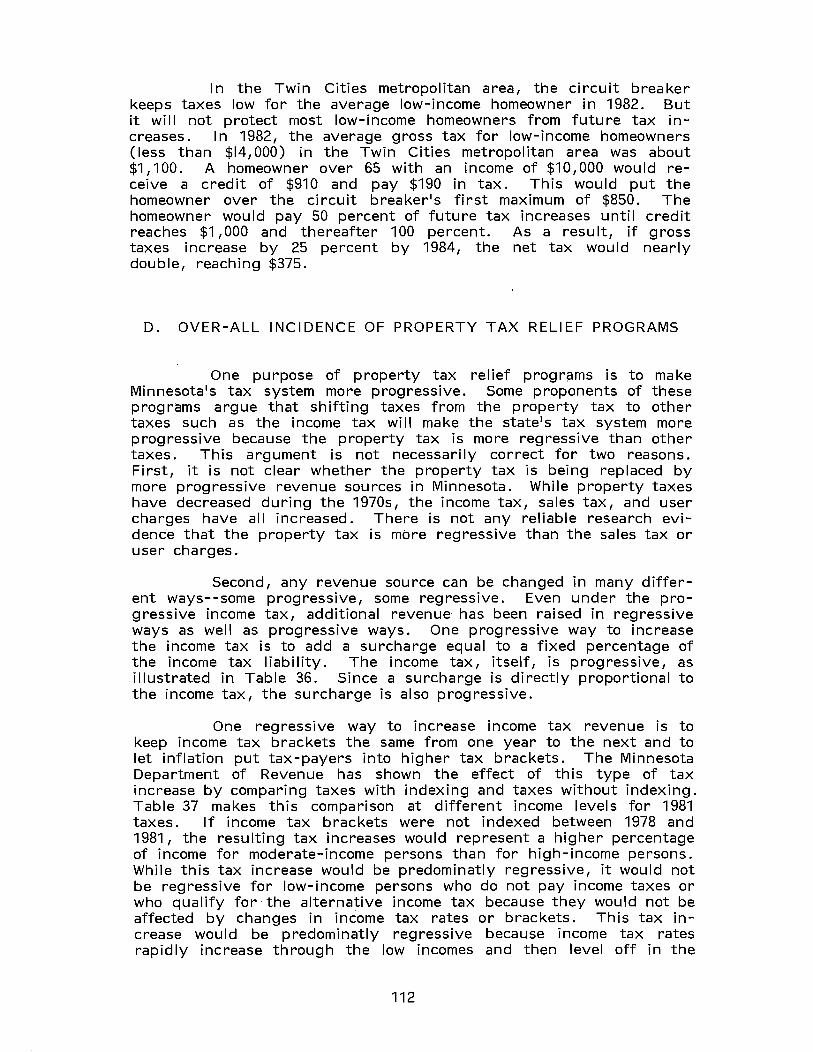
I n the Twin Cities metropolitan area, the circuit breaker keeps taxes low for the average low-income homeowner in 1982. But it will not protect most low-income homeowners from future tax in­creases. In 1982, the average gross tax for low-income homeowners (less than $14,000) in the Twin Cities metropolitan area was about $1,100. A homeowner over 65 with an income of $10,000 would re­ceive a credit of $910 and pay $190 in tax. This would put the homeowner over the circuit breaker1s first maximum of $850. The homeowner would pay 50 percent of future tax increases until credit reaches $1,000 and thereafter 100 percent. As a result, if gross taxes increase by 25 percent by 1984, the net tax would nearly double, reaching $375.

D. OVER-ALL INCIDENCE OF PROPERTY TAX RELIEF PROGRAMS

One purpose of property tax relief programs is to make Minnesota1s tax system more progressive. Some proponents of these programs argue that shifting taxes from the property tax to other taxes such as the income tax will make the state1s tax system more progressive because the property tax is more regressive than other taxes. This argument is not necessarily correct for two reasons. First, it is not clear whether the property tax is being replaced by more progressive revenue sources in Minnesota. While property taxes have decreased during the 1970s, the income tax, sales tax, and user charges have all increased. There is not any reliable research evi­dence that the property tax is more regressive than the sales tax or user charges.

Second, any revenue source can be changed in many differ­ent ways--some progressive, some regressive. Even under the pro­gressive income tax, additional revenue has been raised in regressive ways as well as progressive ways. One progressive way to increase the income tax is to add a surcharge equal to a fixed percentage of the income tax liability. The income tax, itself, is progressive, as illustrated in Table 36. Since a surcharge is directly proportional to the income tax, the surcharge is also progressive.

One regressive way to increase income tax revenue is to keep income tax brackets the same from one year to the next and to let inflation put tax-payers into higher tax brackets. The Minnesota Department of Revenue has shown the effect of this type of tax increase by comparing taxes with indexing and taxes without indexing. Table 37 makes this comparison at different income levels for 1981 taxes. If income tax brackets were not indexed between 1978 and 1981, the resulting tax increases would represent a higher percentage of income for moderate-income persons than for high-income persons. While this tax increase would be predominatly regressive, it would not be regressive for low-income persons who do not pay income taxes or who qualify for' the alternative income tax because they would not be affected by changes in income tax rates or brackets. This tax in­crease would be predominatly regressive because income tax rates rapidly increase through the low incomes and then level off in the

112

--'

--'

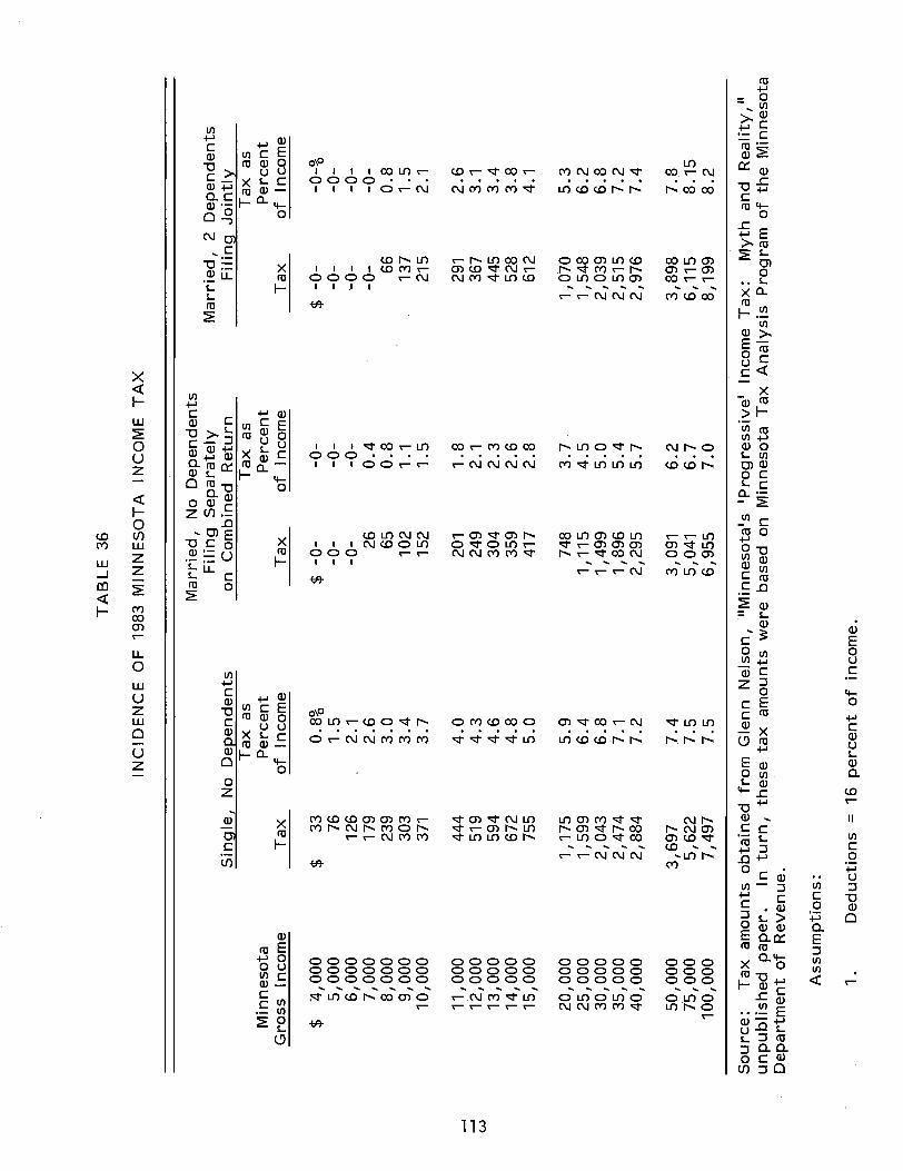
w

TA

BL

E

36

INC

IDE

NC

E

OF

1983

MIN

NE

SO

TA

IN

CO

ME

T

AX

Mar

ried

, N

o D

epen

den

ts

Fil

ing

Sep

arat

ely

M

arri

ed,

2 D

epen

den

ts

Sin

gle

, N

o De~endents

on

Com

bine

d R

etu

rn

Fil

ing

Join

tly:

T

ax a

s T

ax a

s T

ax a

s M

inn

eso

ta

Per

cen

t P

erce

nt

Per

cen

t G

ross

In

com

e T

ax

of

Inco

me

Tax

o

f In

com

e T

ax

of

Inco

me

$ it,

OO

O

$ 33

0.

8%

$ -0

--0

-$

-0-

-0-%

5

,00

0

76

1.5

-0

--0

--0

--0

-6

,00

0

126

2.1

-0

--0

--0

--0

-7

,00

0

179

2.6

26

0

.4

-0-

-0-

8,0

00

23

9 3

.0

65

0.8

66

0

.8

9,0

00

30

3 3

.4

102

1.1

13

7 1

.5

10

,00

0

371

3.7

15

2 1

.5

215

2.1

11

,00

0

444

4.0

20

1 1

.8

291

2.6

1

2,0

00

51

9 4

.3

249

2.1

36

7 3

.1

13

,00

0

594

4.6

30

4 2

.3

445

3.4

1

4,0

00

67

2 4

.8

359

2.6

52

8 3

.8

15

,00

0

755

5.0

41

7 2

.8

612

4.1

20

,00

0

1,1

75

5

.9

748

3.7

1

,07

0

5.3

2

5,0

00

1

,59

9

6.4

1

,11

5

4.5

1

,54

8

6.2

3

0,0

00

2

,04

3

6.8

1

,49

9

5.0

2

,03

9

6.8

3

5,0

00

2

,47

4

7.1

1

,89

6

5.4

2

,51

5

7.2

4

0,0

00

2

,88

4

7.2

2

,29

5

5.7

2

,97

6

7.4

50

,00

0

3,6

97

7

.4

3,09

1 6

.2

3,8

98

7

.8

75

,00

0

5,6

22

7

.5

5,04

1 6

.7

6,1

15

8

.15

1

00

,00

0

7,4

97

7

.5

6,9

55

7

.0

8,1

99

8

.2

So

urc

e:

Tax

am

ou

nts

ob

tain

ed f

rom

G

len

n

Nel

son

, II

Min

neso

tals

IPro

gre

ssiv

el

Inco

me

Tax

: M

yth

and

R

eali

ty,l

I u

np

ub

lish

ed

pap

er.

In

tu

rn,

these

tax

am

ou

nts

w

ere

bas

ed o

n

Min

nes

ota

Tax

An

aly

sis

Pro

gra

m o

f th

e M

inn

eso

ta

Dep

artm

ent

of

Rev

enu

e.

Ass

um

pti

on

s:

1 .

Ded

uct

ion

s =

16 p

erc

en

t o

f in

com

e.

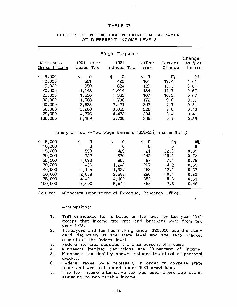
TABLE 37

EFFECTS OF INCOME TAX INDEXING ON TAXPAYERS AT DIFFERENT INCOME LEVELS

Single Taxpayer

Minnesota 1981 Unin- 1981 Differ- Percent Change

as % of Gross Income dexed Tax Indexed Tax ence Change Income

$ 5,000 $ 0 $ 0 $ 0 0% 0% 10,000 521 420 101 19.4 1.01 15,000 950 824 126 1;3.3 0.84 20,000 1,148 1,014 134 11.7 0.67 25,000 1,536 1,369 167 10.9 0.67 30,000 1,908 1,736 172 9.0 0.57 40,000 2,623 2,421 202 7.7 0.51 50,000 3,280 3,052 228 7.0 0.46 75,000 4,776 4,472 304 6.4 0.41

100,000 6,109 5,760 349 5.7 0.35

Family of Four--Two Wage Earners (65%-35% I ncome Split)

$ 5,000 $ 0 $ 0 $ 0 0% 0% 10,000 8 8 0 0 0 15,000 550 429 121 22.0 0.81 20,000 722 579 143 19.8 0.72 25,000 1,092 905 187 17.1 0.75 30,000 1,455 1,248 207 14.2 0.69 40,000 2,195 1,927 268 12.2 0.67 50,000 2,878 2,588 290 10.1 0.58 75,000 4,491 4,109 382 8.5 0.51

100,000 6,000 5,542 458 7.6 0.46

Source: Minnesota Department of Revenue, Research Office.

Assumptions:

1. 1981 unindexed tax is based on tax laws for tax year 1981 except that income tax rate and brackets were from tax year 1978.

2. Taxpayers and families making under $20,000 use the stan­dard deduction at the state level and the zero bracket amounts at the federal level.

3. Federal itemized deductions are 23 percent of income. 4. Minnesota itemized deductions are 20 percent of income. 5. Minnesota tax liability shown includes the effect of personal

credits. 6. . Federal taxes were necessary in order to compute state

taxes and were calculated under 1981 provisions. 7. The low income alternative tax was used where applicable,

assuming no non-taxable income.

114

high incomes. Thus, inflation pushes low-income tax-payers into higher brackets faster than it pushes high-income tax-payers. This means that the income tax became less progressive during the 1970s prior to income tax indexing in 1979. It also means that much of Minnesota's property tax reform was financed in a regressive way rather than in a progressive way as has commonly been assumed.

We conclude from these arguments that it is not clear whether indirect property tax relief programs such as school aids and aid to local government have led to a more progressive or more re­gressive tax system in Minnesota. As a result, justification for these programs should be based on factors other than making the tax system more progressive. However, the incidence of the homestead credit and circuit breaker programs can be more accurately deter­mined. We show below that they have led to a more progressive tax system.

Table 38 compares the incidence of the circuit breaker, homestead credit, and two different income tax increases. I n each case, the incidence is measured in terms of change in tax as a per­centage of income. Several conclusions can be drawn from this table. Together, the homestead credit and circuit breaker are progressive. Total credit as a percentage of income steadily increases as income decreases. Total credit equals about 8 percent of income for house­holds with an income of $5,000, 4 percent for households with an income of $11,000 and less than 2 percent for households with incomes exceeding $31,000. Clearly, these two programs have made the tax system more progressive regardless of which other major revenue sources are used to finance them. Individually, the circuit breaker program is highly progressive and the homestead credit program is progressive, although not nearly as much as the circuit breaker. The circuit breaker is clearly progressive enough to more than offset the possible regressiveness of other taxes used to finance it. The effect of the homestead credit is less clear. If it is financed with an inflation-driven income tax increase, the tax and the credit will to a large extent offset each other.

Furthermore, if the homestead credit were to be reduced, the circuit breaker would often make up deductions in the homestead credit on a dollar for dollar basis, particularly for low income home­owners. For example, changing the maximum homestead credit by $100 affects only homeowners whose income exceeds $23,000. Conse­quently, as shown in Table 38, raising the homestead credit maximum by $100 makes the tax system more regressive, even if it is financed by the progressive income tax surcharge.

115

.;..

..J

--'

. Q

)

TA

BL

E 3

8

CO

MP

AR

ISO

N

OF

IN

CID

EN

CE

F

OR

C

IRC

UIT

B

RE

AK

ER

, H

OM

ES

TE

AD

C

RE

DIT

, IN

CO

ME

T

AX

IN

DE

XIN

G,

AN

D

INC

OM

E

TA

X

SU

RC

HA

RG

E

Pro

pert

y T

ax

Rel

ief

Pro

gra

m

Cre

dit

s A

s In

com

e T

ax

Ch

ang

es A

s A

P

erc

en

t o

f In

com

e,

1982

A

P

erc

en

t o

f In

com

e -

--

--

--

--

--

--

--

--

--

--

--

--

--

--

--

--

--

--

--

--

--

--

10

Perc

en

t C

han

ge

Hom

e-C

han

ge

in

Inco

me

Inco

me

Tax

H

om

este

ad

stead

C

red

it

Tax

D

ue

to

Ind

exin

g

Su

rch

arg

e

Cre

dit

&

Hom

e-M

axim

um

1978

-

1981

* 19

83

Cir

cu

it

Cir

cu

it

stead

fr

om

$6

50

Fam

ily

Fam

ily

Inco

me

Bre

ak

er

Bre

ak

er

Cre

dit

to

$55

0 In

com

e S

ing

le

of

4 o

f 2*

*

$ o

-3

,00

0

17.7

7%

11.7

8%

5.89

%

0%

3,0

00

-

5,0

00

8

.38

5

.54

2

.84

0

$ 3

,00

0

0%

0%

0%

5,0

00

-

10

,00

0

5.7

3

3.2

9

2.4

3

0 5

,00

0

0 0

0

10

,00

0

-1

5,0

00

3

.77

1

.89

1

.87

0

10

,00

0

1.0

1

0 .1

5

15

,00

0 -

20

,00

0

3.0

1

1.1

9

1.8

1

0 1

5,0

00

0

.84

0

.81

.2

8

20

,00

0

-2

5,0

00

2

.14

0

.56

1

.57

.0

1 2

0,0

00

0

.67

0

.72

.3

7

25

,00

0

-3

0,0

00

2

.24

0

.34

1

.89

.0

4

25

,00

0

0.6

7

0.7

5

.45

30

,00

0

-3

5,0

00

1

.94

0

.14

1

.79

.0

9

30

,00

0

0.5

7

0.6

9

.50

35

,00

0

-4

0,0

00

1

.69

0

.05

1

.63

.1

8

35

,00

0

.54

40

,00

0

-4

5,0

00

1

.48

0

.02

1

.45

.1

9

40

,00

0

0.5

1

0.6

7

.57

45

,00

0

-5

0,0

00

1

.32

0

.03

1

.29

.1

8

45

,00

0

50

,00

0

0.4

6

0.5

8

.62

*S

ee T

able

37

for

assu

mp

tio

ns.

*

*M

arri

ed,

no

dep

en

den

ts;

fili

ng

se

para

tely

on

co

mb

ined

fo

rm;

Ded

uct

ion

s =

16 p

erc

en

t o

f in

com

e.

v. POLICY OBJECTIVES IN THE STATE-LOCAL FISCAL RELATIONSHIP

Direct property tax relief programs make up a large part of state aid to local government. In 1982, the homestead credit, agricul­tural credit, taconite homestead credit, reduced assessment credit and other direct property tax relief programs amount to $600 million in aid to local taxing districts. These aids appear as credits onindi­vidual property tax bills, but the money is sent directly to local units of government and school districts in proportion to each taxing dis­trict's share of the property tax levy. An additional $168 million was distributed to individual taxpayers through the circuit breaker pro­gram. Thus, direct property tax relief programs are an important part of the state-local fiscal relationship.

Concern over the state-local fiscal relationship has. b~en spurred by revenue shortfalls and unexpected aid cutbacks, as well as growth in the state's financial commitment to direct property tax relief programs, resulting from legislative decisions made in previous years when the revenue picture was distinctly more positive.

Legislative debate on property taxes and property'tax relief programs is properly part of a broader debate on state aid to local governments. A number of organizations, committees, and lobbies including the Citizens League, Minneapolis Chamber of Commerce, the Association of Minnesota Counties, and the Legislative Local Govern­ment Policy Task Force, along with other individuals and groups have recently issued reports and recommendations designed to reform the state-local fiscal relationship.

There is no reason to expect groups as diverse as these to agree in every particular on the solution to the problem but there is general agreement that there is a problem and that major reform rather than a piecemeal approach needs to pe undertaken.

We feel it is useful to conclude our report on direct prop­erty tax relief programs with a review of the principles on which there is general agreement and then to examine the implications of these generally accepted principles on direct property tax relief programs. The major principles that we feel should guide legislative deliberations during the 1983 session are as follows:

• Minnesota's state-local fiscal system needs comprehensive reform.

There are several reasons why comprehensive reform that goes beyond the immediate budget situation is required. The fiscal strain caused by direct property tax relief programs along with other state aids to local government and schools is long-term rather than temporary in nature. At the same time, fifteen years of active imple­mentation and expansion of state aid programs and direct property tax relief programs have left property taxes in Minnesota low com­pared to where they were historically and in comparison to other

117

states. However, the property tax relief programs are costly, and together form a system that is complex, difficult to understand and poorly understood. I n fact, the growing complexity of the system makes it more and more difficult for the legislature to take action toward any coherent purpose. Further tinkering with the system should be avoided if it adds to the system1s complexity or inadver­tently dilutes the historic commitment of the state to equalization of the ability of schools and local government to provide basic services.

• Greater predictability and stability in state aid is needed by local government. Sudden cuts or increases do not con-tribute to wise spending decisions.

It is now well understood that the state1s major revenue sources are quite volatile and move with the national economy. All state transfers of money to local government are equivalent to a substitute of revenue sources that are unstable for a revenue source (the property tax) that, whatever its faults, is slow to react to economic cycles. While there is general recognition that the state cannot afford to promise growing aid payments in the face of declining revenue, there is no reason to expect initial agreement on the solu­tions to the problem. These include allowing local government and schools greater authority to raise revenue on their own; dedicating a share of state tax revenues to local units rather than a specific dollar amount; and reviewing the totality of state property tax relief pro­grams to see which are expendable in a time of scarcity.

• The state-local fiscal system, including the property tax system, property tax relief programs and other state aid programs, should be simplified in order to improve under­standing of the system in the legislature and among the general public. Simplification is also needed in order to reduce record-keeping costs and to promote uniform classi­fication and assessment practices across the state.

• It is preferable to achieve targeted goals through budgeted expenditures rather than manipulation of the tax system.

Minnesota has the most complex property classification system in the nation with over 50 legal classes of property. It also has a state aid system which is complex and depends on accurate and uniform assessment of property across the state if it is to be fair. Time spent by local assessors classifying property is time that cannot be spent on assessment. Also the administrative cost of accounting for assessed value in a large number of legal classes needs to be weighed against the benefits achieved, although the use of the classi­fication system to accomplish particular objectives is a good way to hide both the costs and benefits of legislative action.

Minnesota also has a wider variety of direct property tax relief programs than any other state, and some of these programs create major administrative headaches at the local level. Without questioning the validity of the objectives of the agricultural credit, powerline credit, wetland or native prairie credits, it can be sug­gested that these purposes could be more easily carried out through direct appropriations, other aid programs or even within the property tax system in a simpler way.

118

• State aid to local government should neither encourage nor discourage local spending. State aid should not provide cheap marginal dollars in support of local levies.

It may be argued that state aid encourages local spending or even requires it. But there is general agreement that it is not desirable to encourage 'spending beyond a certain point or for pur­poses that are not related to the basic services that the state seeks to guarantee. The homestead credit is the best example of a property tax relief program that insulates local government from the full tax consequences of spending decisions and can distort the way in which local government might otherwise choose to raise money. For example, a special assessment might be the best or fairest way to raise money for certain services, but it will not be used if a taxing district can obtain partial state payment through the homestead credit by raising revenue through the property tax levy. I n order to prevent state aid from encouraging local spending, the state has instituted levy limits, but the complex combination of state aids, and variation in local needs and preferences has led to a situation where some local units receive more aid than they need and others are left unable to finance services that most people would regard as basic and essential.

• While often maligned, the property tax is essential because it taxes a form of wealth that would otherwise go untaxed and it is the only significant revenue source now available to local government.

The property tax is one of three broad based taxes avail­able (income and general sales taxes are the others) that raise money by broad application at relatively low rates and it is preferable that revenue be raised through the application of broad based taxes. Also, theoretical and philosophical arguments aside, Minnesota re­quires a mix of revenue sources that is not too different from that of other states, especially neighboring states, if it is to avoid unwanted consequences, especially in border communities.

• Local government is best equipped to deliver a wide range of public services, while equity in taxing and spending dictates that the state carry a major part of the responsi­bility for financing those services. In order to assure that local government is effective and efficient, local government needs a I,arge measure of autonomy in spending decisions, and the ability to raise revenue adequate to finance services demanded, through the political process, by local residents.

• State aid to local government should include incentives to promote efficiency, effectiveness and innovation in the delivery of services.

The principal challenge of a state aid program is to provide aid while not destroying the incentives that make the local administra­tive system work well. The state has a vital role in equalizing local capacity to raise money for certain basic people-related services such as education. At the same time, state aid should not insulate local officials from the consequence of spending decisions, nor prohibit the

119

local electorate and locally elected officials from determining what services (beyond those that the state defines a responsibility for) ought to be available, and at what level they ought to be provided.

• The over-all effect of state and local taxing and spending programs should be progressive. Individual taxes or spending programs need not pass this test, although it is one criterion on which they should be judged.

A related point is that the state-local fiscal system, includ­ing the property tax system and related aids and credits, education and local government aids, levy limits, and other state aids, needs to be considered as a whole while individual components are debated. The result of adhering to this approach should be better coordination among aids, better comprehension of the system in the legislature and among local administrators, and a more effective system in general.

A. IMPLICATIONS FOR DIRECT PROPERTY TAX RELIEF PROGRAMS

The purpose of this brief section is not to reach firm recommendations and conclusions about the direct property tax relief programs that have been the focus of this report, but to make a few obvious connections between these programs and the general principles discussed above.

The homestead credit, as noted earlier, can be criticized because it makes cheap marginal dollars available to local taxing districts and thus can work to encourage a higher local property tax levy than would otherwise be approved.

The homestead credit now costs close to $500 million per year and any reform of the system designed to either save money, improve the effectiveness of state aid programs, equalize resources across the state, or make property tax relief sensitive to income will necessarily have to examine how the dollars now flowing through the homestead credit might be spent more purposefully.

The homestead credit and agricultural credit along with certain other direct property tax relief programs have grown substan­tially in cost over the last fifteen years--mostly because of periodic and even frequent expansion of the programs by the legislature but also because of factors outside direct legislative control, such as growth in real estate values and increases in the cost of providing government services. Since the state's obligation through direct property tax relief programs can grow while state revenue sources are shrinking, direct property tax programs need to be examined if greater stability and predicability in state aids are to be achieved.

Direct property tax relief programs contribute to the com­plexity of the entire property tax system, although individually they are simple compared to the complexity of school and local government aid formulas. This report has demonstrated that while simple in

120

concept, there are significant difficulties in the local administration of the programs. The agricultural credit for agricultural homesteads is computed as the amount of money yielded by multiplying 18, 10 and 8 mills, respectively, against the assessed value of the first 320, next 320 and remaining acreage. Ownership of farms is often in a family or corporation rather than a single person or couple and the location of the land that constitutes an agricultural homestead need not be either contiguous or in the same taxing district. Correct classifica­tion of agricultural and residential property for the purpose of accu­rately computing the agricultural and homestead credits is a problem.

I n addition some direct property tax relief programs such as the wetland credit, native prairie credit, or reduced assessment credit might better be removed from the property tax system alto­gether so that these programs that really have nothing to do with raising revenue can be better evaluated each biennium.

The homestead credit and agricultural credit are not income sensitive; they can and do reduce the taxes of property owners who have the ability to pay a reasonable property tax. Since real prop­erty is a form of wealth and one measure of economic well-being, it is appropriate that it ought not to escape appropriate taxation.

The homestead and agricultural credits are a tool for sub­stituting state for local revenue and since local revenue is almost ex­clusively raised through the property tax, it is a substitute of reve­nue raised through the individual and corporate income taxes, general sales tax and other state sources that are widely thought to be pro­gressive, for revenue raised through the property tax, thought to be a regressive and therefore inferior tax.

We have analyzed the incidence of individual income tax and residential property tax and have concluded that while the homestead credit has a progressive impact on the property tax it is small and aimed at the middle income range. There are more effective means to accomplish this end, such as the circuit breaker. Direct property tax relief programs that merely substitute. state for local revenue should not be assumed to have a uniformly progressive effect because the property tax is less regressive than widely assumed and is prob­ably proportional or even progressive over a significant part of the income range. And, the state individual income tax which has a schedule of nominal rates that appears progressive is only slightly progressive over a broad income range. Other state revenue sources are presumably even less progressive, such as the corporate income tax and general sales tax.

I n summary, we believe direct property tax relief programs can be criticized because they are inconsistent with a number of principles defining what the state-local fiscal relationship should look like. Although they were not included in this study, the same gen­eral point can be made about the present local government aid and school aid programs. We believe a thorough review of the state-local fiscal relationship by the legislature is required and that the princi­ples listed above can provide direction for the effort.

121