evaluation of feynman integrals: advanced methodsriemann/talks/riemann-recap... · 2009-04-02 ·...
TRANSCRIPT

'&
$%
.
Evaluation of Feynman Integrals:Advanced Methods
Getting Ready for Physics at the LHC
Workshop organized by RECAPP at HRI
16–20 Feb. 2009, Allhabad, India
Tord Riemann, DESY, Zeuthen
exercises part: Janusz Gluza, Katowice
J.G
luza
and
T.Rie
mann
–16-2
0Feb
2009
–RECAPP,Alla
habad,In
dia
1

'&
$%
The slides of lecture
and
the files for the exercises
=>
http://www-zeuthen.desy.de/˜riemann/Talks/RECAPP-20 09/
Thanks to
T. Diakonidis
J. Fleischer
K. Kajda
B. Tausk
V. Yundin
J.G
luza
and
T.Rie
mann
–16-2
0Feb
2009
–RECAPP,Alla
habad,In
dia
2

'&
$%
• Introduction + motivation Part 1: 1–36
definitions, general formula for L-loop integrals, Feynman parameter integration
Infrared and ultraviolet divergencies
Few simple Examples
• Mellin-Barnes representations and their evaluation Part 2: 37–63
Numerical and analytical approaches
Expansions in small parameters, e.g. m2/s 63-65
• Expressing Integrals by other integrals (and numerical methods) Part 3: 65–106
Differential equations 65–77
Integration by parts 83–84
Sector decomposition 85–96
Tensor reduction 97–110
Summary 112
• Other methods: skipped
probably skipped: difference equations → Laporta, ”High-precision calculation of multi-loop
Feynman integrals by difference equations” see:[Laporta:2001dd]
Not covered: completely numerical approaches a la Passarino et al. in recent years
J.G
luza
and
T.Rie
mann
–16-2
0Feb
2009
–RECAPP,Alla
habad,In
dia
3
'&
$%
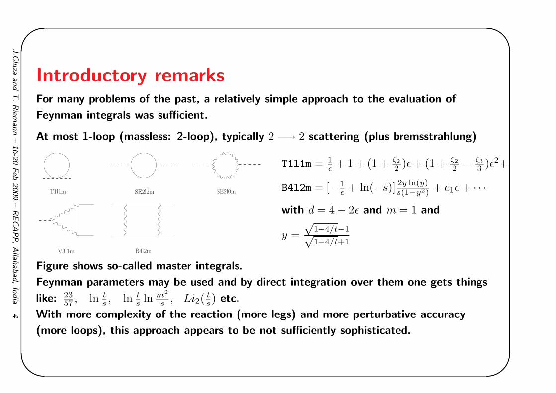
Introductory remarksFor many problems of the past, a relatively simple approach to the evaluation of
Feynman integrals was sufficient.
At most 1-loop (massless: 2-loop), typically 2 −→ 2 scattering (plus bremsstrahlung)
T1l1m SE2l2m
B4l2m
SE2l0m
V3l1m
T1l1m = 1ǫ + 1 + (1 + ζ2
2 )ǫ + (1 + ζ2
2 − ζ3
3 )ǫ2+
B4l2m = [− 1ǫ + ln(−s)] 2y ln(y)
s(1−y2) + c1ǫ + · · ·
with d = 4 − 2ǫ and m = 1 and
y =
√1−4/t−1√1−4/t+1
Figure shows so-called master integrals.
Feynman parameters may be used and by direct integration over them one gets things
like: 2357 , ln t
s , ln ts ln m2
s , Li2(ts ) etc.
With more complexity of the reaction (more legs) and more perturbative accuracy
(more loops), this approach appears to be not sufficiently sophisticated.
J.G
luza
and
T.Rie
mann
–16-2
0Feb
2009
–RECAPP,Alla
habad,In
dia
4

'&
$%
More loops
V6l4m1 V6l4m1d V6l4m2
Two-loop vertex integrals with six internal lines
massless case: only fixed numbers and one scale factor
SE3l2M1m
B5l2M2md B5l2M2m
V4l2M2md
SE3l2M1md
V4l2M1m
V4l2M2m
V4l2M1md
Integrals with two different mass scales m and M
J.G
luza
and
T.Rie
mann
–16-2
0Feb
2009
–RECAPP,Alla
habad,In
dia
5
'&
$%
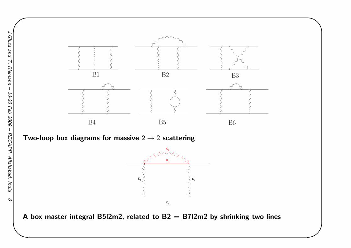
B1 B3B2
B4 B5 B6
Two-loop box diagrams for massive 2 → 2 scattering
K1
K3
K4K2
K5
A box master integral B5l2m2, related to B2 = B7l2m2 by shrinking two lines
J.G
luza
and
T.Rie
mann
–16-2
0Feb
2009
–RECAPP,Alla
habad,In
dia
6

'&
$%
More legs
Massive pentagon: 5 kinematic variables + several masses
Massless and massive hexagons: 8 kinematic variables + several masses
Variables for 2 → 2 scattering, i.e. box diagrams: s, t or s and cos θ
Variables for 2 → 3 scattering: 5 = 2 + 3 (three additional momenta of a particle)
Variables for 2 → 4 scattering: 8 = 5 + 3 (another three additional)
J.G
luza
and
T.Rie
mann
–16-2
0Feb
2009
–RECAPP,Alla
habad,In
dia
7

'&
$%
What are ”Advanced Methods?”
• High degree of automatization
• Publicly available – or not . . .
• Go beyond the methods a la Passarino-Veltman and the relatively simple polylogs
• Not yet completely worked out
• Allow the solution of ”Advanced Problems”
J.G
luza
and
T.Rie
mann
–16-2
0Feb
2009
–RECAPP,Alla
habad,In
dia
8
'&
$%
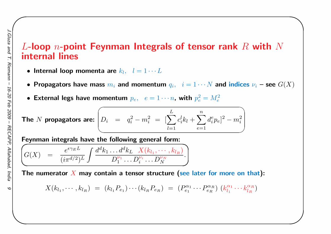
L-loop n-point Feynman Integrals of tensor rank R with Ninternal lines
• Internal loop momenta are kl, l = 1 · · ·L
• Propagators have mass mi and momentum qi, i = 1 · · ·N and indices νi – see G(X)
• External legs have momentum pe, e = 1 · · ·n, with p2e = M2
e
The N propagators are:
Di = q2
i − m2i = [
L∑
l=1
clikl +
n∑
e=1
dei pe]
2 − m2i
Feynman integrals have the following general form:
G(X) =
eǫγEL
(iπd/2)L
∫
ddk1 . . . ddkL X(kl1 , · · · , klR)
Dν11 . . .Dνi
i . . .DνN
N
.
The numerator X may contain a tensor structure (see later for more on that):
X(kl1 , · · · , klR) = (kl1Pe1) · · · (klRPeR) = (Pα1e1
· · ·PαReR
) (kα1
l1· · · kαR
lR)
J.G
luza
and
T.Rie
mann
–16-2
0Feb
2009
–RECAPP,Alla
habad,In
dia
9

'&
$%
Tensor integralsTensor integrals appear naturally in Feynman diagrams, due to
• fermion propagators
• non-abelian triple-boson vertices
• boson propagators in Rξ gauges and unitary gauge
Example: Fermionic vacuum polarization
Παβ ∼ 1
(iπd/2)
∫
ddkTr
[
[γk + m1]
D1γβ [γ(k + p1) + m2]
D2γα
]
∼ 1
(iπd/2)
∫
ddk
D1D2
[
(m1m2 − k2 − kp1)gαβ + 2kαkβ + kαpβ
1 + pα1 kβ
]
So, one needs also efficient ways to evaluate tensor integrals – see later
J.G
luza
and
T.Rie
mann
–16-2
0Feb
2009
–RECAPP,Alla
habad,In
dia
10

'&
$%
Simple examples of scalar integrals
m
A0 =1
(iπd/2)
∫
ddk
D1→ UV − divergent : ∼ d4k
k2
pp
m2
m1
B0 =1
(iπd/2)
∫
ddk
D1D2→ UV − divergent ∼ d4k
k4
m1
m3
m2
p1
p2
p3
C0 =1
(iπd/2)
∫
ddk
D1D2D3→ UV − finite ∼ d4k
k6
Dependent on conventions, where k starts to run in the loop, it is:
D1 = k2 − m21
D2 = (k + p1)2 − m2
2
D3 = (k + p1 + p2)2 − m2
3
J.G
luza
and
T.Rie
mann
–16-2
0Feb
2009
–RECAPP,Alla
habad,In
dia
11

'&
$%
Evaluate Feynman integrals
There are two strategies to solve a Feynman integral:
• Reduction
Express the integral with the aid of recurrence relations by other, known integrals.
These are then the Master Integrals.
• Direct evaluation
J.G
luza
and
T.Rie
mann
–16-2
0Feb
2009
–RECAPP,Alla
habad,In
dia
12

'&
$%
Introduce Feynman parameters
1
Dν11 Dν2
2 . . .DνN
N
=Γ(ν1 + . . . + νN )
Γ(ν1) . . .Γ(νN )
∫ 1
0
dx1 . . .
∫ 1
0
dxNxν1−1
1 . . . xνN−1N δ(1 − x1 . . . − xN )
(x1D1 + . . . + xNDN )Nν,
with Nν = ν1 + . . . νN .
The denominator of G contains, after introduction of Feynman parameters xi, the momentum
dependent function m2 with index-exponent Nν :
(m2)−(ν1+...+νN ) = (x1D1 + . . . + xNDN )−Nν = (kiMijkj − 2Qjkj + J)−Nν
Here M is an (LxL)-matrix, Q = Q(xi, pe) an L-vector and J = J(xixj , m2i , pej
pel).
M, Q, J are linear in xi. The momentum integration is now simple:
Shift the momenta k such that m2 has no linear term in k:
k = k + (M−1)Q,
m2 = kMk − QM−1Q + J.
Remember: M1−loop = 1, in general:
M−1 =1
(det M)M,
where M is the transposed matrix to M . The shift leaves the integral unchanged.
J.G
luza
and
T.Rie
mann
–16-2
0Feb
2009
–RECAPP,Alla
habad,In
dia
13

'&
$%
The shift leaves the integral unchanged (rename k → k):
G(1) =
∫
Dk1 . . .DkL
(kMk + J − QM−1Q)Nν
.
Go Euclidean: Rotate now the k0 → iK0E with k2 → −k2
E (and again rename kE → k):
G(1) → (i)L
∫
DkE1 . . . DkE
L
(−kEMkE + J − QM−1Q)Nν
= (−1)Nν (i)L
∫
Dk1 . . .DkL
[kMk − (J − QM−1Q)]Nν
.
Call
µ2(x) = −(J − QM−1Q)
and get
G(1) = (−1)Nν (i)L
∫
Dk1 . . .DkL
(kMk + µ2)Nν
.
For 1-loop integrals it is L = 1, M = 1 - and we will use nearly only those - we are ready to do the
k-integration.
J.G
luza
and
T.Rie
mann
–16-2
0Feb
2009
–RECAPP,Alla
habad,In
dia
14

'&
$%
Additional step for L-loop integrals
For L-loops go on and now diagonalize the matrix M by a rotation:
k → k′(x) = V (x) k,
kMk = k′Mdiagk′
→∑
αi(x)k2i (x),
Mdiag(x) = (V −1)+MV −1 = (α1, . . . , αL).
This leaves both the integration measure and the integral invariant:
G(1) = (−1)Nν (i)L
∫
Dk1 . . .DkL
(∑
i αik2i + µ2)
Nν.
Rescale now the ki,
ki =√
αiki,
with
ddki = (αi)−d/2ddki,
L∏
i=1
αi = det M,
J.G
luza
and
T.Rie
mann
–16-2
0Feb
2009
–RECAPP,Alla
habad,In
dia
15

'&
$%
and get the Euclidean integral to be calculated (and rename k → k):
G(1) = (−1)Nν (i)L(det M)−d/2
∫
Dk1 . . .DkL
(k21 + . . . + k2
L + µ2)Nν
.
Use now (remembering that Dk = dk/(iπd/2)):
iL∫
Dk1 . . .DkL
(k21 + . . . + k2
L + µ2)Nν
=Γ(
Nν − d2L)
Γ (Nν)
1
(µ2)Nν−dL/2
,
iL∫
Dk1 . . .DkL k21
(k21 + . . . + k2
L + µ2)Nν
=d
2
Γ(
Nν − d2L − 1
)
Γ (Nν)
1
(µ2)Nν−dL/2−1
.
These formulae follow for L = 1 immediately from any textbook.
See ’Mathematical Interlude’.
For L > 1, get it iteratively, with setting (k21 + k2
2 + m2)N = (k21 + M2)N , M2 = k2
2 + m2, etc.
J.G
luza
and
T.Rie
mann
–16-2
0Feb
2009
–RECAPP,Alla
habad,In
dia
16

'&
$%
Mathematical interlude: d-dimensional integrals (I)
After the Wick rotation, the integrand of the momentum integration is positive definite.
Further it is independent of the angular variables.
The integral is understood as symmetric limit the infinity boundaries.∫
ddk kµ F (k2) = 0
∫
ddk F (k + C) =
∫
ddk F (k).
Introduce d-dim. spherical coordinates. The vector k has d components:
kd = r cos θd ≡ ρd cos θd
kd−1 = ρd−1 cos θd−1
. . .
k3 = ρ3 cos θ3
k2 = ρ2 sinφ
k1 = ρ2 cosφ
ρd−1 = ρd sin θd
J.G
luza
and
T.Rie
mann
–16-2
0Feb
2009
–RECAPP,Alla
habad,In
dia
17

'&
$%
Mathematical interlude: d-dimensional integrals (II)
The above is the direct generalization of the 3- or 4-dimensional phase space parametrization.
With these variables, the integral over the complete d-dimensional phase space gets the
following form:
∫ ∞
−∞
ddk F (k) = limR→∞
∫ R
0
drrd−1
∫ π
0
dθd−1 sind−2 θd−1
∫ π
0
dθd−2 sind−3 θd−2 . . .
∫ 2π
0
dθ1F (k)
The integrations met in the loop calculations may be performed using the following two integrals:
∫ π
0
dθ sinm θ =√
πΓ[
12 (m + 1)
]
Γ[
12 (m + 2)
] ,
∫ ∞
0
drrβ
(r2 + M2)α=
1
2
Γ(
β+12
)
Γ(
α − β+12
)
Γ (α)
1
(M2)α−(β+1)/2
.
In general, the angular integrations are influenced by the integrand too. (Remember phase space
integrals of bremsstrahlung!)
J.G
luza
and
T.Rie
mann
–16-2
0Feb
2009
–RECAPP,Alla
habad,In
dia
18

'&
$%
Mathematical interlude: d-dimensional integrals (III)
If F (k) → F (r), r = |k|, the angular integrations yield the surface of the d-dimensional sphere
with radius r:
ωd(r) =2πd/2
Γ[
d2
] rd−1.
The remaining integration, over r, yields for F (r) = 1 the volume of the sphere with radius R:
Vd(R) =πd/2
Γ[
1 + d2
]Rd,
G(1) =
∫
ddk1
(k2 + M2)Nν
.
=
∫ ∞
0
drωd(r)
(r2 + M2)Nν
and we get immediately, with M2 ≡ M2(x1, x2, . . .):
G(1) =
[
iπd/2Γ (Nν − d/2)
Γ(Nν)
1
(M2)Nν−d/2
]
.
J.G
luza
and
T.Rie
mann
–16-2
0Feb
2009
–RECAPP,Alla
habad,In
dia
19

'&
$%
The Γ-function
The Γ-function may be defined by a difference equation:
zΓ(z) − Γ(z + 1) = 0
Γ(z) =
∫ ∞
0
tz−1e−tdt
Series[Gamma[ep], ep, 0, 2] =
Γ[ǫ] =1
ǫ− γE +
1
12(6γE
2 + π2)ǫ +1
12(−2γE
3 − γE2π + 2Ψ(2, 1))ǫ2 + · · ·
Ψ(2, 1)) = PolyGamma(2, 1) = −2ζ3
exp(ep EulerGamma)Series[Gamma[ep], ep, 0, 2] =
eǫγEΓ[ǫ] =1
ǫ+
1
12(π2)ǫ +
1
6(Ψ(2, 1))ǫ2 + · · ·
J.G
luza
and
T.Rie
mann
–16-2
0Feb
2009
–RECAPP,Alla
habad,In
dia
20

'&
$%
Look at the singularities in the complex plane (figure shows real part of Γ):
When applying the Cauchy-theorem, one may close the integral to the left or to the right . . .
J.G
luza
and
T.Rie
mann
–16-2
0Feb
2009
–RECAPP,Alla
habad,In
dia
21
'&
$%
Mathematical interlude: d-dimensional integrals (IV)
We will often use:
aǫ = eǫ ln a = 1 + ǫ ln a + . . .
J.G
luza
and
T.Rie
mann
–16-2
0Feb
2009
–RECAPP,Alla
habad,In
dia
22
'&
$%
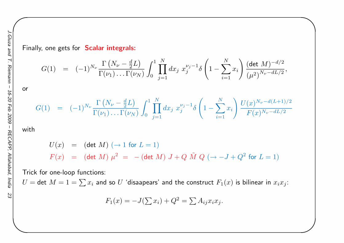
Finally, one gets for Scalar integrals:
G(1) = (−1)NνΓ(
Nν − d2L)
Γ(ν1) . . .Γ(νN )
∫ 1
0
N∏
j=1
dxj xνj−1j δ
(
1 −N∑
i=1
xi
)
(det M)−d/2
(µ2)Nν−dL/2
,
or
G(1) = (−1)NνΓ(
Nν − d2L)
Γ(ν1) . . .Γ(νN )
∫ 1
0
N∏
j=1
dxj xνj−1j δ
(
1 −N∑
i=1
xi
)
U(x)Nν−d(L+1)/2
F (x)Nν−dL/2
with
U(x) = (det M) (→ 1 for L = 1)
F (x) = (det M) µ2 = − (det M) J + Q M Q (→ −J + Q2 for L = 1)
Trick for one-loop functions:
U = det M = 1 =∑
xi and so U ‘disaapears’ and the construct F1(x) is bilinear in xixj :
F1(x) = −J(∑
xi) + Q2 =∑
Aijxixj .
J.G
luza
and
T.Rie
mann
–16-2
0Feb
2009
–RECAPP,Alla
habad,In
dia
23

'&
$%
The vector integral differs by some numerator kipe and thus there is a single shift in the integrand
k → k + U(x)−1MQ
theR
ddk k/(k2 + µ2) → 0, and no further changes:
G(k1α) = (−1)NνΓ`
Nν −d2L´
Γ(ν1) . . . Γ(νN )
Z 1
0
NY
j=1
dxj xνj−1
j δ
1 −
NX
i=1
xi
!
U(x)Nν−d(L+1)/2−1
F (x)Nν−dL/2
"
X
l
M1lQl
#
α
,
Here also a tensor integral:
G(k1αk2β) = (−1)Nν
Γ`
Nν − d2 L´
Γ(ν1) . . . Γ(νN )
Z 1
0
NY
j=1
dxj xνj−1
j δ
1 −
NX
i=1
xi
!
U(x)Nν−2−d(L+1)/2
F (x)Nν−dL/2
×X
l
"
[M1lQl]α[M2lQl]β −Γ`
Nν − d2 L − 1
´
Γ`
Nν − d2 L´
gαβ
2U(x)F (x)
(V −11l )+(V −1
2l )
αl
#
.
The 1-loop case will be used in the following L times for a sequential treatment of an L-loop
integral (remember∑
xjDj = k2 − 2Qk + J and F (x) = Q2 − J):
G([1, kpe]) = (−1)NνΓ(
Nν − d2
)
Γ(ν1) . . .Γ(νN )
∫ 1
0
N∏
j=1
dxj xνj−1j δ
(
1 −N∑
i=1
xi
)
[1, Qpe]
F (x)Nν−d/2
J.G
luza
and
T.Rie
mann
–16-2
0Feb
2009
–RECAPP,Alla
habad,In
dia
24

'&
$%
Examples for one-loop F -polynomials
One-loop vertex:
F (t, m2) = m2(x1 + x2)2 + [−t]x1x2
one-loop box:
F (s, t, m2) = m2(x1 + x2)2 + [−t]x1x2 + [−s]x3x4
one-loop pentagon:
F (s, t, t′, v1, v2, m2) = m2(x1 + x3 + x4)
2 + [−t]x1x3 + [−t′]x1x4 + [−s]x2x5 + [−v1]x3x5 + [−v2]x2x4
2-loop example: B7l4m2, has a box-type sub-loop with 2 off-shell legs:
F−(a4567−d/2) =
[−t]x4x7 + [−s]x5x6 + m2(x5 + x6)2
+(m2 − Q21)x7(x4 + 2x5 + x6) + (m2 − Q2
2)x7x5
−(a4567−d/2)
2-loop: B5l2m2, sub-loop with 2 off-shell legs (diagram see p.4):
F2lines(k21, m
2) = m2(x3)2 + [−k2
1 + m2]x1x3
J.G
luza
and
T.Rie
mann
–16-2
0Feb
2009
–RECAPP,Alla
habad,In
dia
25

'&
$%
The Tadpole A0(m)
m
T1l1m[a] = A0 =eǫγE
(iπd/2)
∫
ddk
(k2 − m2)a→ UV − divergent
With our general formulae we get, in the 1-dimensional Feynman parameter integral,
for the numerator
N = (k2 − m2)x1 ≡ k2 + J
F = m2x1 ≡ m2x21
and thus
T1l1m[a] = (−1)aeǫγEΓ[a − d/2]
Γ[a]
∫ 1
0
dxxa−1δ[1 − x]1
F a−d/2
= (−1)aeǫγE (m2)2−a−ǫ Γ[a − 2 + ǫ]
Γ[a]
→ −eǫγEΓ[−1 + ǫ] for a = 1, m = 1
=1
ǫ+ 1 +
(
1 +ζ2
2
)
ǫ +
(
1 +ζ2
2− ζ3
3
)
ǫ2 + · · ·
J.G
luza
and
T.Rie
mann
–16-2
0Feb
2009
–RECAPP,Alla
habad,In
dia
26

'&
$%
The Self-energy B0(s,m1,m2)
pp
m2
m1
SE2l = B0[s, m1, m2] = (2√
πµ)4−d eǫγE
(iπd/2)
∫
ddk
[k2 − m2][(k + p)2 − m22]
The SE2l is UV-divergent and the corresponding F -function is:
F [s, m1, m2] = m21x
21 + m2
2x22 − [s − m2
1 − m22]x1x2
and for special cases:
F [s, m1, 0] = m21x
21 − [s − m2
1]x1x2
F [s, m1, m1] = m21(x1 + x2)
2 − [s]x1x2
F [s, 0, 0] = −[s]x1x2
The ’conventional’ Feynman parameter integral is 1-dimensional because x2 ≡ 1 − x1:
F (x) = −sx(1 − x) + m22(1 − x) + m2
1x ≡ −s(x − xa)(x − xb)
J.G
luza
and
T.Rie
mann
–16-2
0Feb
2009
–RECAPP,Alla
habad,In
dia
27
'&
$%
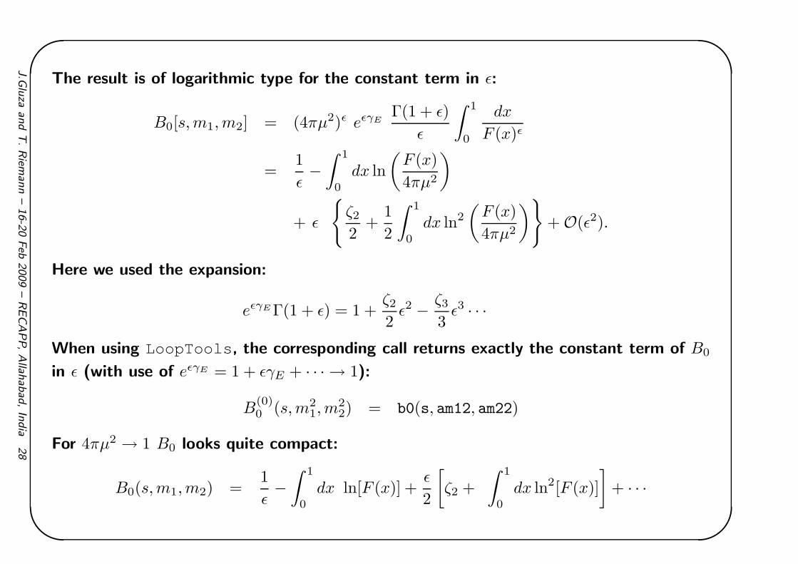
The result is of logarithmic type for the constant term in ǫ:
B0[s, m1, m2] = (4πµ2)ǫ eǫγEΓ(1 + ǫ)
ǫ
∫ 1
0
dx
F (x)ǫ
=1
ǫ−∫ 1
0
dx ln
(
F (x)
4πµ2
)
+ ǫ
ζ2
2+
1
2
∫ 1
0
dx ln2
(
F (x)
4πµ2
)
+ O(ǫ2).
Here we used the expansion:
eǫγE Γ(1 + ǫ) = 1 +ζ2
2ǫ2 − ζ3
3ǫ3 · · ·
When using LoopTools , the corresponding call returns exactly the constant term of B0
in ǫ (with use of eǫγE = 1 + ǫγE + · · · → 1):
B(0)0 (s, m2
1, m22) = b0(s, am12, am22)
For 4πµ2 → 1 B0 looks quite compact:
B0(s, m1, m2) =1
ǫ−∫ 1
0
dx ln[F (x)] +ǫ
2
[
ζ2 +
∫ 1
0
dx ln2[F (x)]
]
+ · · ·
J.G
luza
and
T.Rie
mann
–16-2
0Feb
2009
–RECAPP,Alla
habad,In
dia
28

'&
$%
Explicitly, one has to integrate
ln[F (x)] = ln[−s(x − xa)(x − xb)]
ln2[F (x)] = ln2[−s(x − xa)(x − xb)]
So we will need the integrals:∫
dx10 ln(x − xa), ln(x − xa)ln(x − xb)
which is trivial, together with some complex algebra rules how to handle complex
arguments of logarithms with
s → s + iǫ
wherever needed.
J.G
luza
and
T.Rie
mann
–16-2
0Feb
2009
–RECAPP,Alla
habad,In
dia
29

'&
$%
For the case m1 = m2 = 1, one gets for the first terms in ǫ:
B0[s, 1, 1] =1
ǫ+ 2 +
1 + y
1 − yH(0, y),
H(0, y) = ln(y).
The H(0, y) is a harmonic polylogarithmic function, and
y =
√−s + 4 −
√−s√
−s + 4 +√−s
s = − (1 − x)2
x
The other case treated later again is m1 = 0, m2 = m:
B0[s, m2, 0] =
1
ǫ+ 2 +
1 − s/m2
s/m2ln(1 − s/m2)
J.G
luza
and
T.Rie
mann
–16-2
0Feb
2009
–RECAPP,Alla
habad,In
dia
30

'&
$%
The massive one-loop vertex C0(s,m1,m2)
m1
m3
m2
p1
p2
p3
C0 =eǫγE
(iπd/2)
∫
ddk
[(k + p1)2 − m2][k2][(k − p2)2 − m2]∼ |k→∞
d4k
k6→ UV − fin.
The massive vertex (all m1, m2, m3 6= 0) is a finite quantity.
We assume immediately m1 = m3 = 0.
A problem now is IR-divergence.
Appears when a massive internal line is between two external on-shell lines.
Incoming p21 = m2 and p2
2 = m2, look at k → 0:
d4k1
(k − p2)2 − m2
1
(k)21
(k + p1)2 − m2
= d4k1
k2 − 2kp2
1
(k)21
k2 + 2kp1
→ d4k
k1+2+1∼ k3dk
k4∼ dk
k|k→0 −→ div
An IR-regularization is needed, must take d > 4.
Both UV-div (with d < 4) and IR-div together: must allow for a complex d = 4− 2ǫ, and
take limit at the end.
J.G
luza
and
T.Rie
mann
–16-2
0Feb
2009
–RECAPP,Alla
habad,In
dia
31

'&
$%
First we have a look, for later use, at the F -function:
N = D1x + D2y + D3z
= k2x + (k2 + 2kp1)y + (k2 − 2kp2)z
= k2(x + y + z) + 2k(p1y − p2z)
= (k + Q)2 − Q2
We used 1 = x + y + z here. And the F -function is F = Q2 − J = Q2 (there is no
constant term in N here), as was shown before:
F = m2(y + z)2 + [−s]yz
This F -function does not factorize in y and z. But now back to the direct Feynman
parameter integration.
J.G
luza
and
T.Rie
mann
–16-2
0Feb
2009
–RECAPP,Alla
habad,In
dia
32

'&
$%
Start with change y → y′ = (1 − x)y, then y′ → y:
1
D1D2D3=
∫ 1
0
dxdydzδ(1 − x − y − z)
(D2x + D1y + D3z)3
=
∫ 1
0
dx
∫ 1−x
0
dy
(D2x + D1y + D3z)3
=
∫ 1
0
dx
∫ 1
0
xdy
(D2x + D1y + D3z)3
After this change of variables, the integrand factorizes in x and y:
N = (k + xpy)2 − x2p2y
= (k + Q)2 − Q2
resulting into
F = Q2 = x2p2y
p2y = −sy(1 − y) + m2
J.G
luza
and
T.Rie
mann
–16-2
0Feb
2009
–RECAPP,Alla
habad,In
dia
33

'&
$%
For C0 we obtain (with Nν = 3 and Nν − d/2 = 1 + ǫ):
C0[s, m, m, 0] = (−1)eǫγEΓ[1 + ǫ]
∫ 1
0
dx
x1+2ǫ
∫ 1
0
dy
(p2y)1−ǫ
This is integrable for ǫ < 0, or d > 4, or more general: d ≮ 4.
The x-integral made simple here:
∫ 1
0
dx
x1+2ǫ=
x−2ǫ|10−2ǫ
= −1−2ǫ − 0−2ǫ
2ǫ
= − 1
2ǫ
We see that the IR-singularity is an end-point-singularity in Feynman parameter space.
Further:
− 1
2ǫ
dy
(p2y)1−ǫ
= − 1
2ǫ
dy
(p2y)
(y2)ǫ
= − 1
2ǫ
dy
(p2y)
eǫ ln(y2)
= − 1
2ǫ
dy
(p2y)
[
1 + ǫ ln(y2) + ǫ2 ln2(y2) + · · ·]
Here I stop this study.
J.G
luza
and
T.Rie
mann
–16-2
0Feb
2009
–RECAPP,Alla
habad,In
dia
34

'&
$%
We see that the further integrations proceed quite similar as for the 2-point function, in
fact the p2y = −sy(1 − y) + m2 is the same building block.
The integrals to be solved now are more general, they include also denominators 1/p2y:
Some integrals
∫
dy ln(y − y0) = (y − y0) ln(y − y0) − y + C
∫
dy1
y − y0= ln(y − y0) + C
∫
dyln(y − y0)
y − y0=
1
2ln2(y − y0) + C
Here, often y is real and y0 is complex. Then no special care about phases is necessary.
∫ 1
0
dx
x − x0[ln(x − xA) − ln(x0 − xA)] = Li2
(
x0
x0 − xA
)
− Li2
(
x0 − 1
x0 − xA
)
.
This formula is valid if x0 is real.
J.G
luza
and
T.Rie
mann
–16-2
0Feb
2009
–RECAPP,Alla
habad,In
dia
35

'&
$%
C0 with a small photon mass λIn
[Berends:1976zp,’tHooft:1979xw]
, the C0-integral is treated with a finite photon mass:
∫
d4k
(k2 − λ2)(k2 + 2kp1)(k2 − 2kp2)
= −iπ2
∫ 1
0
dydxy
x2p2y + (1 − x)λ2
= iπ2
∫ 1
0
dy
[
1
2p2y
lnλ2
p2y
+ O(
λ/√
p2y
)
]
,
It is easy to see from the term 1/(2p2y) ln(λ2) the correspondence of (d − 4) and λ2,
which is a universal relation in all 1-loop cases.
16.02.2009: End of Lecture 1.
J.G
luza
and
T.Rie
mann
–16-2
0Feb
2009
–RECAPP,Alla
habad,In
dia
36

'&
$%
Now using Mellin-Barnes Representations
Perform the x-integrations
Find an as-general-as-possible general formula
Make it ready for algorithmic analytical and/or numerical evaluation
Computercodes:
• Ambre.m - Derive Mellin-Barnes representations for Feynman integrals[Gluza:2007rt]
• MB.m - Find an ǫ-expansion and evaluate numerically in Euclidean region[Czakon:2005rk]
J.G
luza
and
T.Rie
mann
–16-2
0Feb
2009
–RECAPP,Alla
habad,In
dia
37

'&
$%
Integrating the Feynman parameters – get MB-Integrals
We derived:
SE2l1m = B0(s, m, 0) = eǫγE Γ(ǫ)
∫ 1
0
dx1dx2δ(1 − x1 − x2)δ(1 − x1 − x2)
F (x)ǫ
V 3l2m = C0(s, m, m, 0) = eǫγE Γ(1 + ǫ)
∫ 1
0
dx1dx2dx3δ(1 − x1 − x2 − x3)
F (x)1+ǫ
and
FSE2l1m = m2x21 − (s − m2)x1x2
FV 3l2m = m2(x1 + x2)2 − (s)x1x2
We want to apply now:
∫ 1
0
N∏
j=1
dxj xαj−1j δ
(
1 −∑
xi
)
=Γ(α1)Γ(α2) · · ·Γ(α7N)
Γ (α1 + α2 + · · · + αN )
with coefficients αi dependent on νi and on the structure of the F
See in a minute:For this, we have to apply one or several MB-integrals here.
J.G
luza
and
T.Rie
mann
–16-2
0Feb
2009
–RECAPP,Alla
habad,In
dia
38

'&
$%
∫ 1
0
N∏
j=1
dxj xαj−1j δ
(
1 −N∑
i=1
xi
)
=
∏Ni=1 Γ(αi)
Γ(
∑Ni=1 αi
)
Simplest cases:
∫ 1
0
dx1 xα1−11 δ (1 − x1) = 1
∫ 1
0
2∏
j=1
dxj xαj−1j δ
(
1 −N∑
i=1
xi
)
=
∫ 1
0
dx1xα1−11 (1 − x1)
α2−1 = B(α1, α2)
=Γ(α1)Γ(α2)
Γ (α1 + α2)
J.G
luza
and
T.Rie
mann
–16-2
0Feb
2009
–RECAPP,Alla
habad,In
dia
39

'&
$%
Here we want to go:
1
(A + B)λ=
1
Γ(λ)
1
2πi
∫ +i∞
−i∞
dzΓ(λ + z)Γ(−z)Bz
Aλ+z
The formula looks a bit unusual to loop people, but for persons with a mathematical
background it is common.
J.G
luza
and
T.Rie
mann
–16-2
0Feb
2009
–RECAPP,Alla
habad,In
dia
40
'&
$%
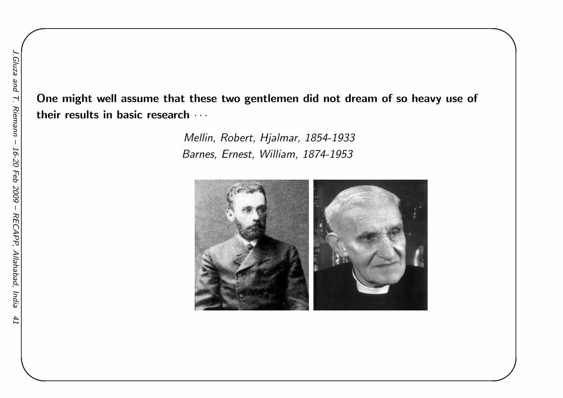
One might well assume that these two gentlemen did not dream of so heavy use of
their results in basic research · · ·
Mellin, Robert, Hjalmar, 1854-1933
Barnes, Ernest, William, 1874-1953
J.G
luza
and
T.Rie
mann
–16-2
0Feb
2009
–RECAPP,Alla
habad,In
dia
41

'&
$%
.
Barnes’ contour integrals for the hypergeometric function
Exact proof and further reading: Whittaker & Watson (CUP 1965) 14.5 - 14.52, pp.
286-290
Consider
F (z) =1
2πi
∫ +i∞
−i∞
dσ(−z)σ Γ(a + σ)Γ(b + σ)Γ(−σ)
Γ(c + σ)
where |arg(−z)| < π (i.e. (−z) is not on the neg. real axis) and the path is such that it
separates the poles of Γ(a + σ)Γ(b + σ) from the poles of Γ(−σ).
1/Γ(c + σ) has no pole.
Assume a 6= −n and b 6= −n, n = 0, 1, 2, · · · so that the contour can be drawn.
The poles of Γ(σ) are at σ = −n, n = 1, 2, · · · , and it is:
Residue[ F[s] Gamma[-s] , s,n ] = (-1)ˆn/n! F(n)
Closing the path to the right gives then, by Cauchy’s theorem, for |z| < 1 the
J.G
luza
and
T.Rie
mann
–16-2
0Feb
2009
–RECAPP,Alla
habad,In
dia
42

'&
$%
hypergeometric function 2F1(a, b, c, z) (for proof see textbook):
1
2πi
∫ +i∞
−i∞
dσ(−z)σ Γ(a + σ)Γ(b + σ)Γ(−σ)
Γ(c + σ)=
N→∞∑
n=0
Γ(a + n)Γ(b + n)
Γ(c + n)
zn
n!
=Γ(a)Γ(b)
Γ(c)2F1(a, b, c, z)
The continuation of the hypergeometric series for |z| > 1 is made using the
intermediate formula
F (z) =
∞∑
n=0
Γ(a + n)Γ(1 − c + a + n) sin[(c − a − n)π]
Γ(1 + n)Γ(1 − a + b + n) cos(nπ) sin[(b − a − n)π](−z)−a−n
+
∞∑
n=0
Γ(b + n)Γ(1 − c + b + n) sin[(c − b − n)π]
Γ(1 + n)Γ(1 − a + b + n) cos(nπ) sin[(a − b − n)π](−z)−b−n
and yields
Γ(a)Γ(b)
Γ(c)2F1(a, b, c, z) =
Γ(a)Γ(a − b)
Γ(a − c)(−z)−a
2F1(a, 1 − c + a, 1 − b + ac, z−1)
+Γ(b)Γ(b − a)
Γ(b − c)(−z)−b
2F1(b, 1 − c + b, 1 − a + b, z−1)
J.G
luza
and
T.Rie
mann
–16-2
0Feb
2009
–RECAPP,Alla
habad,In
dia
43

'&
$%
Corollary I
Putting b = c, we see that
2F1(a, b, b, z) =
∞∑
n=0
Γ(a + n)
Γ(a)
zn
n!
=1
(1 − z)a=
1
2πi Γ(a)
∫ +i∞
−i∞
dσ (−z)σ Γ(a + σ)Γ(−σ)
This allows to replace sum by product:
1
(A + B)a=
1
Ba[1 − (−A/B)]a=
1
2πiΓ(a)
i∞∫
−i∞
dσAσ B−σ−a Γ(a + σ)Γ(−σ)
J.G
luza
and
T.Rie
mann
–16-2
0Feb
2009
–RECAPP,Alla
habad,In
dia
44

'&
$%
Barnes’ lemma
If the path of integration is curved so that the poles of Γ(c − σ)Γ(d − σ) lie on the right
of the path and the poles of Γ(a + σ)Γ(b + σ) lie on the left, then
1
2πi
∫ +i∞
−i∞
dσΓ(a + σ)Γ(b + σ)Γ(c − σ)Γ(d − σ) =Γ(a + c)Γ(a + d)Γ(b + c)Γ(b + d)
Γ(a + b + c + d)
It is supposed that a, b, c, d are such that no pole of the first set coincides with any pole
of the second set.
Scetch of proof: Close contour by semicircle C to the right of imaginary axis. The
integral exists and∫
Cvanishes when ℜ(a + b + c + d − 1) < 0. Take sum of residues of
the integrand at poles of Γ(c − σ)Γ(d − σ). The double sum leads to two
hypergeometric functions, expressible by ratios of Γ-functions, this in turn by
combinations of sin, may be simplifies finally to the r.h.s.
Analytical continuation: The relation is proved when ℜ(a + b + c + d − 1) < 0.
Both sides are analytical functions of e.g. a. So the relation remains true for all values
of a, b, c, d for which none of the poles of Γ(a + σ)Γ(b + σ), as a function of σ, coincide
with any of the poles of Γ(c − σ)Γ(d − σ).
Corollary II Any real shift k: σ + k, a − k, b − k, c + k, d + k together with∫ −k+i∞
−k−i∞leaves
the result true.
J.G
luza
and
T.Rie
mann
–16-2
0Feb
2009
–RECAPP,Alla
habad,In
dia
45

'&
$%
How can the Mellin-Barnes formula be made useful in thecontext of Feynman integrals?
• Apply corollary I to propagators and get:
1
(p2 − m2)a=
1
2πi Γ(a)
i∞∫
−i∞
dσ(−m2)σ
(p2)a+σΓ(a + σ)Γ(−σ)
which transforms a massive propagator to a massless one (with index a of the line changed
to (a + σ)).
• Apply corollary I after introduction of Feynman parameters and after the momentum
integration to the resulting F - and U -forms, in order to get a single monomial in the xi,
which allows the integration over the xi:
1
[A(s)xa11 + B(s)xb1
1 xb22 ]a
=1
2πi Γ(a)
i∞∫
−i∞
dσ[A(s)xa11 ]σ[B(s)xb1
1 xb22 ]a+σ Γ(a + σ)Γ(−σ)
Both methods leave Mellin-Barnes (MB-) integrals to be performed afterwards.
J.G
luza
and
T.Rie
mann
–16-2
0Feb
2009
–RECAPP,Alla
habad,In
dia
46

'&
$%
A short remark on history
• N. Usyukina, 1975: ”ON A REPRESENTATION FOR THREE POINT FUNCTION”, Teor.
Mat. Fiz. 22;
a finite massless off-shell 3-point 1-loop function represented by 2-dimensional MB-integral
• E. Boos, A. Davydychev, 1990: ”A Method of evaluating massive Feynman integrals”,
Theor. Math. Phys. 89 (1991);
N-point 1-loop functions represented by n-dimensional MB-integral
• V. Smirnov, 1999: ”Analytical result for dimensionally regularized massless on-shell double
box”, Phys. Lett. B460 (1999);
treat UV and IR divergencies by analytical continuation: shifting contours and taking
residues ’in an appropriate way’
• B. Tausk, 1999: ”Non-planar massless two-loop Feynman diagrams with four on-shell legs”,
Phys. Lett. B469 (1999);
nice algorithmic approach to that, starting from search for some unphysical space-time
dimension d for which the MB-integral is finite and well-defined
• M. Czakon, 2005 (with experience from common work with J. Gluza and TR): ”Automatized
analytic continuation of Mellin-Barnes integrals”, Comput. Phys. Commun. (2006);
Tausk’s approach realized in Mathematica program MB.m, published and available for use
J.G
luza
and
T.Rie
mann
–16-2
0Feb
2009
–RECAPP,Alla
habad,In
dia
47

'&
$%
The Γ-function
The Γ-function may be defined by a difference equation:
zΓ(z) − Γ(z + 1) = 0
Γ(z) =
∫ ∞
0
tz−1e−tdt
Series[Gamma[ep], ep, 0, 2] =
Γ[ǫ] =1
ǫ− γE +
1
12(6γE
2 + π2)ǫ +1
12(−2γE
3 − γE2π + 2Ψ(2, 1))ǫ2 + · · ·
Ψ(2, 1)) = PolyGamma(2, 1) = −2ζ3
exp(ep EulerGamma)Series[Gamma[ep], ep, 0, 2] =
eǫγEΓ[ǫ] =1
ǫ+
1
12(π2)ǫ +
1
6(Ψ(2, 1))ǫ2 + · · ·
J.G
luza
and
T.Rie
mann
–16-2
0Feb
2009
–RECAPP,Alla
habad,In
dia
48

'&
$%
Look at the singularities in the complex plane:
When applying the Cauchy-theorem, one may close the integral to the left or to the right . . .
J.G
luza
and
T.Rie
mann
–16-2
0Feb
2009
–RECAPP,Alla
habad,In
dia
49

'&
$%
Some facts on residua
The function
F (z) =
∞∑
i=−N
ai
(z − z0)i
has the residue
Res F (z)|z=z0 = a−1
An integral over an anti-clockwize directed closed path C around z0 then is
1
2πi
∫
C
dzF (z) = 2πia−1
If G(z) has a Taylor expansion around z0 and F (z) has a Laurent expansion beginning with
a−N/(z − z0)N + . . ., then their product has the residue:
Res[G(z) F (z)]|z=z0 =
N∑
k=1
a−kG(z0)(k)
k!
J.G
luza
and
T.Rie
mann
–16-2
0Feb
2009
–RECAPP,Alla
habad,In
dia
50

'&
$%
Some residua with Γ(z) and Ψ(z)
Ψ(z) = PolyGamma[z] = PolyGamma[0, z] → See also next slide
Residue[F[z]Gamma[z], z, -n] = (−1)n
n! F [−n]
Residue[F[z]Gamma[z]2, z, -n] = 2PolyGamma[n+1]F [−n]+F ′[−n](n!)2
Residue[F[z]Gamma[z - 1]2, z, -3] = 25F [−3]−12γEF [−3]+6F ′[−3]3456
F[z] = F [−3]576(z+3)2 + 25F [−3]−12γEF [−3]+6F ′[−3]
3456(z+3)
+ a0 + a1(z + 3) + · · ·Series[Gamma[z + a]Gamma[z - 1]2, z, -3, -1 ] = Γ[−3+a]
576(z+3)2
+ (25Γ[−3+a]−12γEΓ[−3+a]+6(Γ[−3+a]PolyGamma[0,−3+a])3456 + a0 + a1(z + 3) + · · ·
J.G
luza
and
T.Rie
mann
–16-2
0Feb
2009
–RECAPP,Alla
habad,In
dia
51

'&
$%
Where
Polygamma[n + 1] ≡ Polygamma[0, n + 1]
= Ψ(n + 1) =Γ′(n + 1)
Γ(n + 1)= S1(n) − γE =
n∑
k=1
1
k− γE
The following properties hold:
Ψ(z + 1) = Ψ(z) + 1/z
Ψ(1 + ǫ) = −γE + ζ2 ǫ + . . .
Ψ(1) = −γE
Ψ(2) = 1 − γE
Ψ(3) = 3/2 − γE
PolyGamma[n, z] =∂n
∂znΨ(z)
J.G
luza
and
T.Rie
mann
–16-2
0Feb
2009
–RECAPP,Alla
habad,In
dia
52
'&
$%
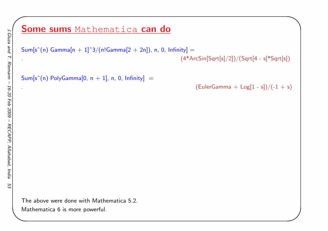
Some sums Mathematica can do
Sum[sˆ(n) Gamma[n + 1]ˆ3/(n!Gamma[2 + 2n]), n, 0, Infinity] =
. (4*ArcSin[Sqrt[s]/2])/(Sqrt[4 - s]*Sqrt[s])
Sum[sˆ(n) PolyGamma[0, n + 1], n, 0, Infinity] =
. (EulerGamma + Log[1 - s])/(-1 + s)
The above were done with Mathematica 5.2.
Mathematica 6 is more powerful.
J.G
luza
and
T.Rie
mann
–16-2
0Feb
2009
–RECAPP,Alla
habad,In
dia
53

'&
$%
A self-energy: SE2l1m
This is a nice example, being simple but showing [nearly] all essentials in a nutshell.
We get for this F (x) = m2x21 − (s − m2)x1x2 the following representation:
SE2l1m =eǫγE
2πi
(m2)−ǫ
Γ[2 − 2ǫ]
∫
ℜz=−1/8
dz
[−s + m2
m2
]−ǫ−z
Γ1[1 − ǫ − z]Γ2[−z]Γ3[1 − ǫ + z]Γ4[ǫ + z]
Tausk approach:
Seek a configuration where all arguments of Γ-functions have positive real part. Then the
SE2l1m is well-defined and finite.
For small ǫ this is - here - evidently impossible; set ǫ → 0 and look at Γ2[−z]Γ4[+z]:
Γ1[1 − z]Γ2[−z]Γ3[1 − +z]Γ4[+z]
What to do ????
Tausk: Set ǫ such that it happens, e.g.:
ǫ = 3/8
To make physics we have now to deform the integrand or the path such that ǫ → 0; when
crossing a residue, take it and add it up.
J.G
luza
and
T.Rie
mann
–16-2
0Feb
2009
–RECAPP,Alla
habad,In
dia
54

'&
$%
Varying ǫ → 0 from 3/8 makes crossing in Γ4[ǫ+ z] a pole at ǫ = −z = +1/8; there is ǫ+ z = 0:
Residue[SE2l1m, z,−ǫ] = eǫγE(m2)−ǫ
Γ[2 − 2ǫ]Γ1[1 − 2ǫ]Γ2[ǫ]
Here we ’loose’ one integration (easier term!) and catch the IR-singularity in Γ2[ǫ] ∼ 1/ǫ!
The function becomes now, for small ǫ:
SE2l1m =eǫγE
2πi
(m2)−ǫ
Γ[2 − 2ǫ]
∫
ℜz=−1/8
dz
[−s + m2
m2
]−ǫ−z
Γ1[1 − ǫ − z]Γ2[−z]Γ3[1 − ǫ + z]Γ4[ǫ + z]
+ eǫγE(m2)−ǫ
Γ[2 − 2ǫ]Γ1[1 − 2ǫ]Γ2[ǫ]
Now we may take the limit of small ǫ because the integral will stay finite and well-defined:
SE2l1m =eǫγE
2πi
∫
ℜz=−1/8
dz
[−s + m2
m2
]−z
Γ3[1 − z]Γ4[−z]Γ[z]Γ[1 + z] + eǫγE
(
2 +1
ǫ− ln[m2]
)
+
Now we close the integration path to the left, catch all residues from Γ3[1 − z] for ℜz < −1/8,
i.e. at z = −n, n = 1, 2, . . .:
Residue
[−s + m2
m2
]−z
Γ1[1 − ǫ − z]Γ2[−z]Γ3[1 − ǫ + z]Γ4[ǫ + z], z,−n
= (−s + m2)n ln(−s + m
J.G
luza
and
T.Rie
mann
–16-2
0Feb
2009
–RECAPP,Alla
habad,In
dia
55

'&
$%
The sum to be done is trivial (in this trivial case!!):
∞∑
n=1
[−s + m2
m2
]n
=1
1 − −s+m2
m2
− 1
and we end up with:
SE2l1m =1
ǫ+ 2 +
[
1 − s/m2
s/m2ln(1 − s/m2)
]
This is what we had also from the direct Feynman parameter integration above
J.G
luza
and
T.Rie
mann
–16-2
0Feb
2009
–RECAPP,Alla
habad,In
dia
56
'&
$%
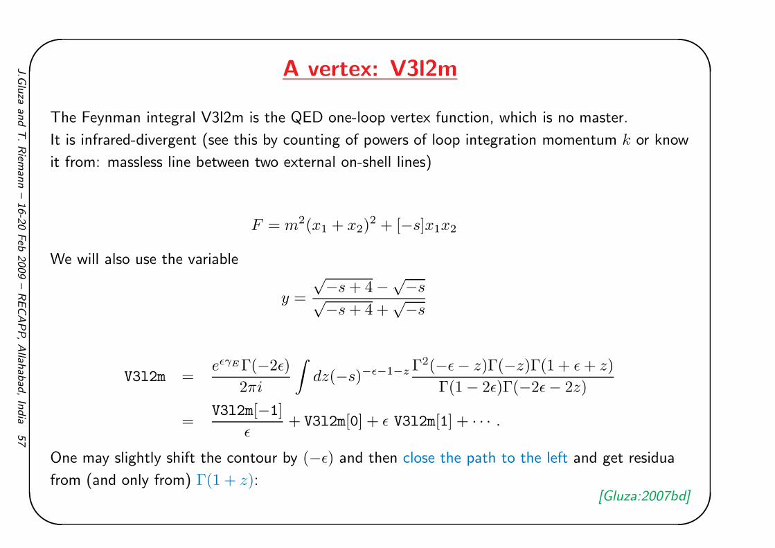
A vertex: V3l2m
The Feynman integral V3l2m is the QED one-loop vertex function, which is no master.
It is infrared-divergent (see this by counting of powers of loop integration momentum k or know
it from: massless line between two external on-shell lines)
F = m2(x1 + x2)2 + [−s]x1x2
We will also use the variable
y =
√−s + 4 −
√−s√
−s + 4 +√−s
V3l2m =eǫγEΓ(−2ǫ)
2πi
∫
dz(−s)−ǫ−1−z Γ2(−ǫ − z)Γ(−z)Γ(1 + ǫ + z)
Γ(1 − 2ǫ)Γ(−2ǫ− 2z)
=V3l2m[−1]
ǫ+ V3l2m[0] + ǫ V3l2m[1] + · · · .
One may slightly shift the contour by (−ǫ) and then close the path to the left and get residua
from (and only from) Γ(1 + z):[Gluza:2007bd]
J.G
luza
and
T.Rie
mann
–16-2
0Feb
2009
–RECAPP,Alla
habad,In
dia
57
'&
$%
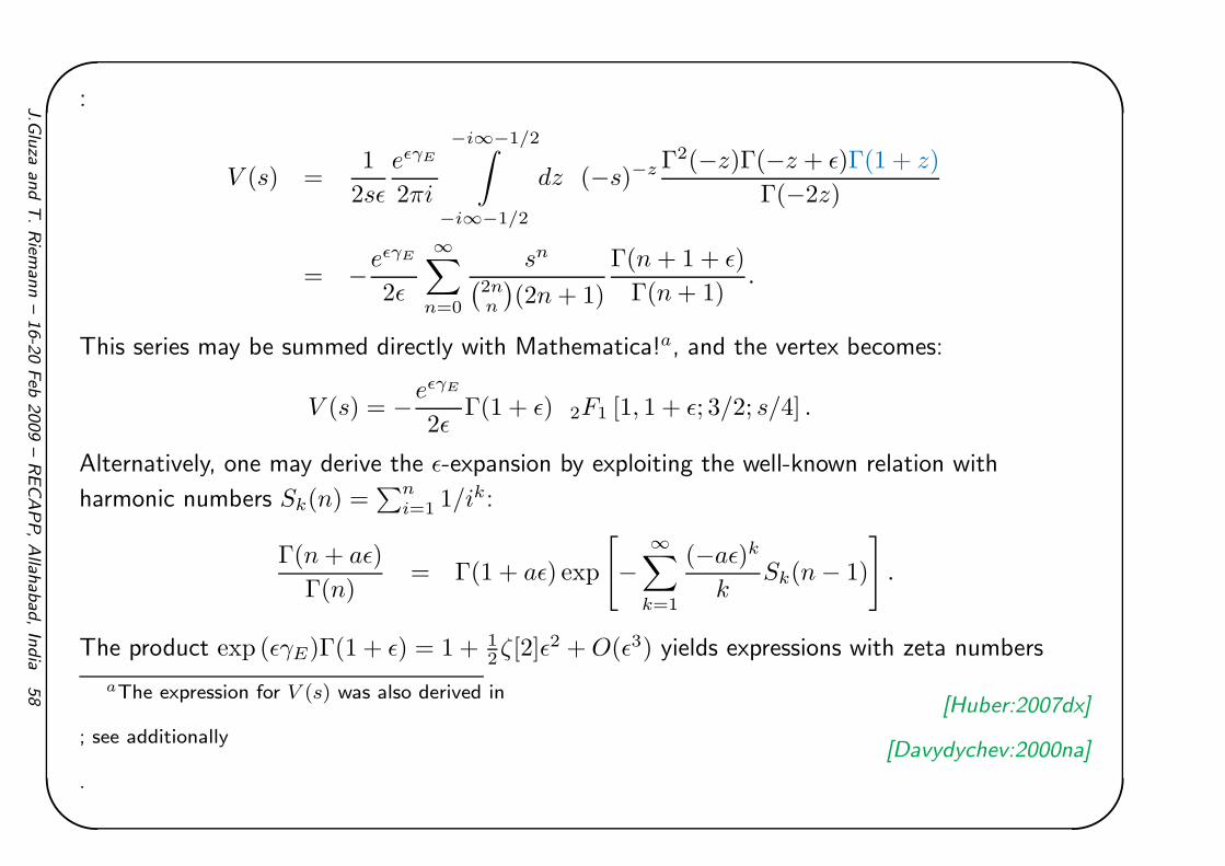
:
V (s) =1
2sǫ
eǫγE
2πi
−i∞−1/2∫
−i∞−1/2
dz (−s)−z Γ2(−z)Γ(−z + ǫ)Γ(1 + z)
Γ(−2z)
= −eǫγE
2ǫ
∞∑
n=0
sn
(
2nn
)
(2n + 1)
Γ(n + 1 + ǫ)
Γ(n + 1).
This series may be summed directly with Mathematica!a, and the vertex becomes:
V (s) = −eǫγE
2ǫΓ(1 + ǫ) 2F1 [1, 1 + ǫ; 3/2; s/4] .
Alternatively, one may derive the ǫ-expansion by exploiting the well-known relation with
harmonic numbers Sk(n) =∑n
i=1 1/ik:
Γ(n + aǫ)
Γ(n)= Γ(1 + aǫ) exp
[
−∞∑
k=1
(−aǫ)k
kSk(n − 1)
]
.
The product exp (ǫγE)Γ(1 + ǫ) = 1 + 12ζ[2]ǫ2 + O(ǫ3) yields expressions with zeta numbers
aThe expression for V (s) was also derived in[Huber:2007dx]
; see additionally[Davydychev:2000na]
.
J.G
luza
and
T.Rie
mann
–16-2
0Feb
2009
–RECAPP,Alla
habad,In
dia
58

'&
$%
ζ[n], and, taking all terms together, one gets a collection of inverse binomial sumsb; the first of
them is the IR divergent part:
V (s) =V−1(s)
ǫ+ V0(s) + · · ·
V−1(s) =1
2
∞∑
n=0
sn
(
2nn
)
(2n + 1)=
1
2
4 arcsin(√
s/2)√4 − s
√s
=y
y2 − 1ln(y).
bFor the first four terms of the ǫ-expansion in terms of inverse binomial sums or of polylogarithmic functions,
see[Gluza:2007bd]
.
J.G
luza
and
T.Rie
mann
–16-2
0Feb
2009
–RECAPP,Alla
habad,In
dia
59

'&
$%
The constant term:
V3l2m[0] =1
2πi
∫ +i∞+u
−i∞+u
dr(−s)−1−r Γ3[−r]Γ[1 + r]
Γ[−2r]
1
2[γE − ln(−s) + 2Ψ[−2r] − 2Ψ[−r] + Ψ[1 + r]]
=1
2
∞∑
n=0
sn
2n
n
(2n + 1)
S1(n),
There is also the opportunity to evaluate the MB-integrals numerically by following with e.g. a
Fortran routine the straight contour.
This applies after the ǫ-expansion.
∫ +5i+ℜz
−5i+ℜzis usually sufficient.
But: This works fast and stable for Euclidean kinematics where −s > 0.
J.G
luza
and
T.Rie
mann
–16-2
0Feb
2009
–RECAPP,Alla
habad,In
dia
60

'&
$%
and the ǫ-term:
V3l2m[1] =1/4
2πi
∫ +i∞+u
−i∞+u
dr(−s)−1−r Γ3[−r]Γ[1 + r]
Γ[−2r)][
γ2E + Log[−s]2 + Log[−s](−2γE − 4Ψ[−2z] + 4Ψ[−z] − 2Ψ[1 + z])
+γE(4Ψ[−2z] − 4Ψ[−z] + 2Ψ[1 + z])
−4Ψ[1,−2z] + 2Ψ[1,−z] + Ψ[1, 1 + z]
+4(Ψ[−2z]2 − 2Ψ[−2z]Ψ[−z] + Ψ[−z]2 + Ψ[−2z]Ψ[1 + z]
−Ψ[−z]Ψ[1 + z]) + Ψ[1 + z]2]
= [const = 1?] × 1
4
∞∑
n=0
(t)n
2n
n
(2n + 1)
[
S1(n)2 + ζ2 − S2(n)]
.
Here, Ψ[r] = ... and Ψ[1, r] = ..., and the harmonic numbers Sk(n) are
Sk(n) =n∑
i=1
1
ik,
J.G
luza
and
T.Rie
mann
–16-2
0Feb
2009
–RECAPP,Alla
habad,In
dia
61

'&
$%
The sums appearing above may be obtained from sums listed in Table 1 of Appendix D in[Gluza:2007bd,Davydychev:2003mv]
:
∞∑
n=0
sn
(
2nn
)
(2n + 1)=
y
y2 − 12 ln(y),
∞∑
n=0
sn
(
2nn
)
(2n + 1)S1(n) =
y
y2 − 1[−4Li2(−y) − 4 ln(y) ln(1 + y) + ln2(y) − 2ζ2
]
,
∞∑
n=0
sn
(
2nn
)
(2n + 1)S1(n)2 =
y
y2 − 1
[
16S1,2(−y) − 8Li3(−y) + 16Li2(−y) ln(1 + y)
+8 ln2(1 + y) ln(y) − 4 ln(1 + y) ln2(y) +1
3ln3(y) + 8ζ2 ln(1 + y)
−4ζ2 ln(y) − 8ζ3
]
,
∞∑
n=0
sn
(
2nn
)
(2n + 1)S2(n) = − y
3(y2 − 1)ln3(y),
J.G
luza
and
T.Rie
mann
–16-2
0Feb
2009
–RECAPP,Alla
habad,In
dia
62

'&
$%
Expansion in a small parameter: vertex V3l2m for m2/s
Use as an example for determining the small mass expansion:
V 3coefm1 = Coefficient[V 3l2m[[1, 1]], ǫ,−1]
= − 1
2s
1
2πi
∫ +i∞−1/2
−i∞−1/2
dz
(
−m2
s
)zΓ1[−z]3Γ2[1 + z]
Γ3[−2z]
If |m2/s| << 1, then the smallest power of it gives the biggest contribution, i.e. its exponent
has to be positive and small.
So, close the contour to the right (positive ℜz), and leading terms come from the residua
expansion of Γ1[−z]3/Γ3[−2z] at z = −1,−2, · · · . The residues are terms of a binomial sum:
Residue = −1
s
(
m2
s
)n(2n)!
(n!)2
[
2HarmonicNumber[n] − 2HarmonicNumber[2n] − ln
(
−m2
s
)]
with first terms equal to (-1)*Residua:
V 3l2m =1
sln
(
−m2
s
)
+m2
s2
[
ln
(
2 + 2m2
s
)]
+m4
s3
[
ln
(
7 + 6m2
s
)]
+ O(m6/s3)
J.G
luza
and
T.Rie
mann
–16-2
0Feb
2009
–RECAPP,Alla
habad,In
dia
63

'&
$%
.Another nice box with numerator, B5l3m(pe.k1)
We used it for the determination if the small mass expansion.
B5l3m(pe · k1) =m4ǫ(−1)a12345 e2ǫγE
Q5j=1 Γ[ai]Γ[5 − 2ǫ − a123](2πi)4
Z
+i∞
−i∞
dα
Z
+i∞
−i∞
dβ
Z
+i∞
−i∞
dγ
Z
+i∞
−i∞
dδ
(−s)(4−2 ǫ)−a12345−α−β−δ
(−t)δ
Γ[−4 + 2 ǫ + a12345 + α + β + δ]
Γ[6 − 3 ǫ − a12345 − α]
Γ[−α] Γ[−β]
Γ[7 − 3 ǫ − a12345 − α] Γ[5 − 2 ǫ − a123]
Γ[−δ]
Γ[4 − 2 ǫ − a1123 − 2 α − γ] Γ[5 − 2 ǫ − a1123 − 2 α
Γ[2 − ǫ − a13 − α − γ]
Γ[8 − 4 ǫ − a112233445 − 2 α − 2 β − 2 δ − γ]
Γ[4 − 2 ǫ − a12345 − α − β − δ − γ]
Γ[9 − 4 ǫ − a112233445 − 2 α − 2 β − 2 δ − γ]
(pe · p3) Γ[1 + a4 + δ] Γ[6 − 3 ǫ −
Γ[4 − 2 ǫ − a1234 − α − β − δ] Γ[3 − ǫ − a12 − α] Γ[8 − 4 ǫ − a112233445 − 2 α − 2 δ − γ]Γ[9 − 4 ǫ − a112233445 − 2 α − 2 β − 2
Γ[5 − 2 ǫ − a1123 − γ] Γ[4 − 2 ǫ − a1123 − 2 α − γ] Γ[a1 + γ] Γ[−2 + ǫ + a123 + α + δ + γ] + Γ[a4 + δ]
»
−(pe · p1) Γ[7 − 3 ǫ − a
Γ[4 − 2 ǫ − a1234 − α − β − δ]Γ[8 − 4 ǫ − a112233445 − 2 α − 2 δ − γ]Γ[9 − 4 ǫ − a112233445 − 2 α − 2 β − 2 δ − γ]»
Γ[3 − ǫ − a12 − α] Γ[5 − 2 ǫ − a1123 − γ]Γ[4 − 2 ǫ − a1123 − 2 α − γ] Γ[a1 + γ] + Γ[2 − ǫ − a12 − α] Γ[4 − 2 ǫ − a1123 − γ]
Γ[5 − 2 ǫ − a1123 − 2 α − γ] Γ[1 + a1 + γ]
–
Γ[−2 + ǫ + a123 + α + δ + γ] + Γ[6 − 3 ǫ − a12345 − α] Γ[3 − ǫ − a12 − α]
Γ[5 − 2 ǫ − a1123 − γ] Γ[4 − 2 ǫ − a1123 − 2 α − γ]Γ[a1 + γ]
»
((pe · (p1 + p2)) Γ[5 − 2 ǫ − a1234 − α − β − δ]Γ[9 − 4 ǫ − a112233445
Γ[8 − 4 ǫ − a112233445 − 2 α − 2 β − 2 δ − γ]Γ[−2 + ǫ + a123 + α + δ + γ] + (pe · p1) Γ[4 − 2 ǫ − a1234 − α − β − δ]
Γ[8 − 4 ǫ − a112233445 − 2 α − 2 δ − γ]Γ[9 − 4 ǫ − a112233445 − 2 α − 2 β − 2 δ − γ]Γ[−1 + ǫ + a123 + α + δ + γ]
–ff
J.G
luza
and
T.Rie
mann
–16-2
0Feb
2009
–RECAPP,Alla
habad,In
dia
64

'&
$%
Differential equations: Example V3l2mExample V3l2m, the massive QED 1-loop vertex
m1
m3
m2
p1
p2
p3
V 3l2m =
Z
ddk
D1D2D3
D1 = (k + p1)2− m2
1
D2 = (k − p2)2− m2
2
D3 = (k)2 − m20
s = (p1 + p2)2 = 2p1p2 + p2
1 + p22
Dimensional arguments prove:
V 3l2m ∼ 1
sat s → ∞
J.G
luza
and
T.Rie
mann
–16-2
0Feb
2009
–RECAPP,Alla
habad,In
dia
65
'&
$%
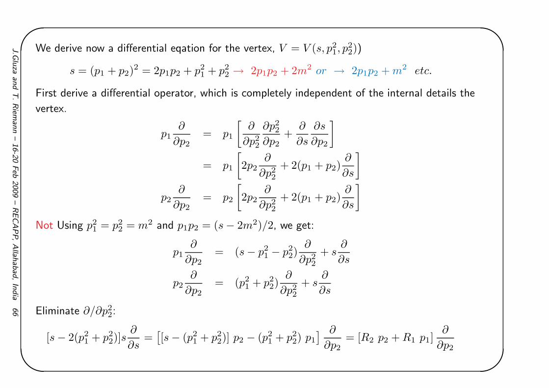
We derive now a differential eqation for the vertex, V = V (s, p21, p
22))
s = (p1 + p2)2 = 2p1p2 + p2
1 + p22 → 2p1p2 + 2m2 or → 2p1p2 + m2 etc.
First derive a differential operator, which is completely independent of the internal details the
vertex.
p1∂
∂p2= p1
[
∂
∂p22
∂p22
∂p2+
∂
∂s
∂s
∂p2
]
= p1
[
2p2∂
∂p22
+ 2(p1 + p2)∂
∂s
]
p2∂
∂p2= p2
[
2p2∂
∂p22
+ 2(p1 + p2)∂
∂s
]
Not Using p21 = p2
2 = m2 and p1p2 = (s − 2m2)/2, we get:
p1∂
∂p2= (s − p2
1 − p22)
∂
∂p22
+ s∂
∂s
p2∂
∂p2= (p2
1 + p22)
∂
∂p22
+ s∂
∂s
Eliminate ∂/∂p22:
[s − 2(p21 + p2
2)]s∂
∂s=[
[s − (p21 + p2
2)] p2 − (p21 + p2
2) p1
] ∂
∂p2= [R2 p2 + R1 p1]
∂
∂p2
J.G
luza
and
T.Rie
mann
–16-2
0Feb
2009
–RECAPP,Alla
habad,In
dia
66

'&
$%
Now apply this universal differential vertex-operator to a specific vertex, e.g. V =V3l2m:
Use on-mass-shell condition p21 = m2
1, p22 = m2
2.
∂V
∂p2=
∫
ddk
D3D1
∂
∂p2
1
D2
With
∂
∂p2
1
D2= − 1
D22
∂D2
∂p2=
2(k − p2)
D22
Compensate numerator against propagators:
2p1k = −D3 + D1 − m20 − p2
1 + m21
2p2k = D3 − D2 + m20 + p2
2 − m22
p2i = m2
i
p1p2 = (s − m21 − m2
2)/2
we get, for this vertex, the equation:
(s − 2(m21 + m2
2)) s∂V
∂s= s
∫
ddk
D1D22
− (m21 + m2
2)
∫
ddk
D3D22
− (s − (m21 + m2
2)) V
There might also arise a dotted Vertex at the right hand side, but here it drops out from the
J.G
luza
and
T.Rie
mann
–16-2
0Feb
2009
–RECAPP,Alla
habad,In
dia
67

'&
$%
result; in general:
[
s − 2(p21 + p2
2)]
s∂
∂s=
∫
dk
[
−R2
D1D2D3+
R2 − R1
D1D22
+R1
D22D3
+R2(m
20 − m2
2 − p22) + R1(−m2
0 + p22 + m2
1 − s)
D1D22D3
]
J.G
luza
and
T.Rie
mann
–16-2
0Feb
2009
–RECAPP,Alla
habad,In
dia
68
'&
$%
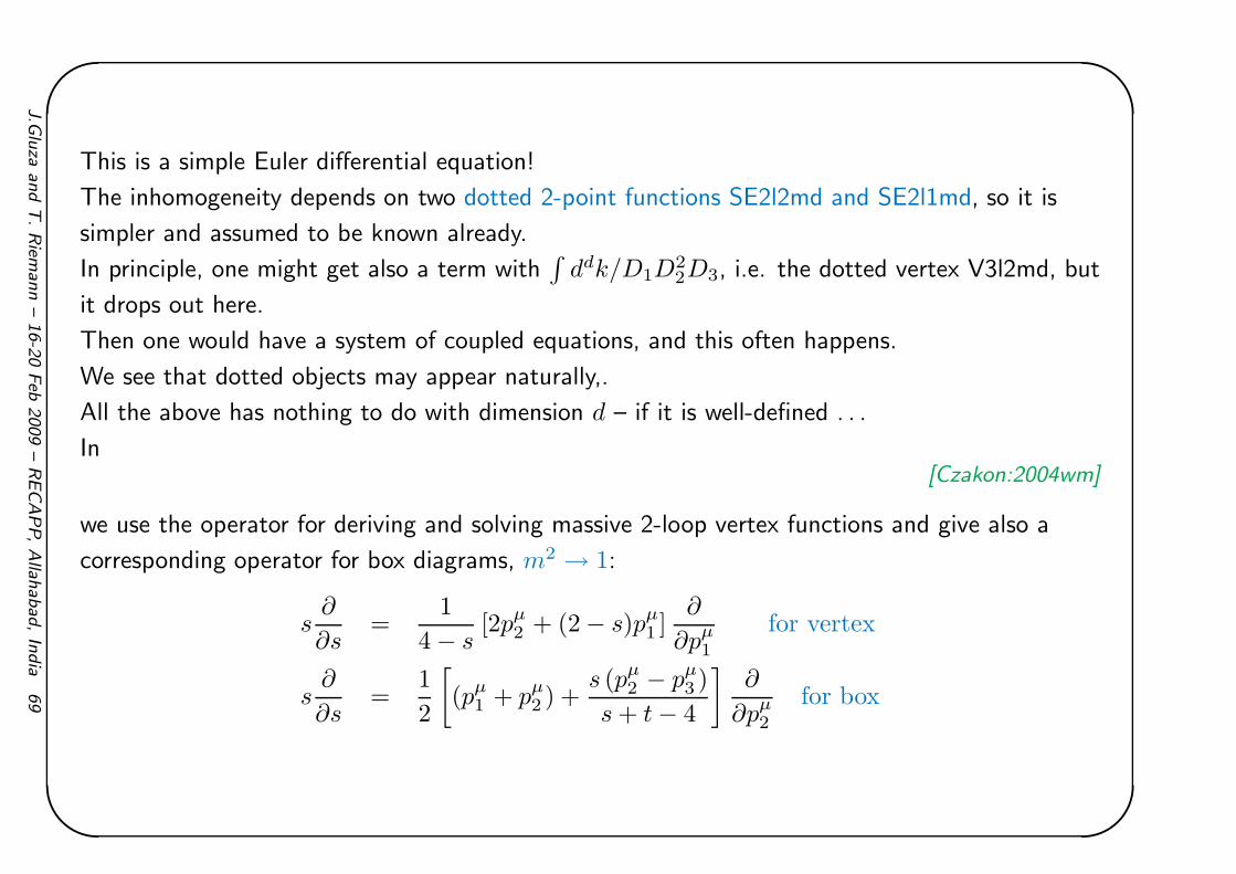
This is a simple Euler differential equation!
The inhomogeneity depends on two dotted 2-point functions SE2l2md and SE2l1md, so it is
simpler and assumed to be known already.
In principle, one might get also a term with∫
ddk/D1D22D3, i.e. the dotted vertex V3l2md, but
it drops out here.
Then one would have a system of coupled equations, and this often happens.
We see that dotted objects may appear naturally,.
All the above has nothing to do with dimension d – if it is well-defined . . .
In[Czakon:2004wm]
we use the operator for deriving and solving massive 2-loop vertex functions and give also a
corresponding operator for box diagrams, m2 → 1:
s∂
∂s=
1
4 − s[2pµ
2 + (2 − s)pµ1 ]
∂
∂pµ1
for vertex
s∂
∂s=
1
2
[
(pµ1 + pµ
2 ) +s (pµ
2 − pµ3 )
s + t − 4
]
∂
∂pµ2
for box
J.G
luza
and
T.Rie
mann
–16-2
0Feb
2009
–RECAPP,Alla
habad,In
dia
69

'&
$%
Scetch of: Solve Euler Diff. EquationsBasics developed in
[Kotikov:1991hm,Kotikov:1991kg,Laporta:1996mq]
. The choice of variables depends on the problem.
For the QED vertex it will prove useful to take
s/m2 = −(1 − x)2/x
For our other beloved example B ≡ B0(s, m, 0), see nice lecture[Aglietti:2004vs]
s/m2 = −x
For details, I prefer to jump to this case.
Differential operator:
s∂
∂s=
1
2pµ ∂
∂pµ
The equation becomes here:
∂
∂sB =
[
− 1
x+
1
1 + x
]
B + ǫ
[
1
x− 2
1 + x
]
B + (1 − ǫ)
[
1
x− 1
1 + x
]
T1l1m
T1l1m =1
ǫ+ 1 + (1 + ζ2/2)ǫ + . . .
J.G
luza
and
T.Rie
mann
–16-2
0Feb
2009
–RECAPP,Alla
habad,In
dia
70

'&
$%
We need also a boundary condition; look at explicit expression above:
B0(0, m, 0) = T1l1m
Make an ansatz as series in ǫ:
B =1
ǫB1 + B0 + ǫB1 + . . .
and get a series of equations:
∂
∂sB−1 = A0B−1 + Ω−1
∂
∂sB0 = A0B0 + A1B−1 + Ω0
∂
∂sB1 = A0B1 + A1B0 + Ω1
etc
J.G
luza
and
T.Rie
mann
–16-2
0Feb
2009
–RECAPP,Alla
habad,In
dia
71

'&
$%
It is:
A0 = − 1
x+
1
1 + x
A1 =1
x− 2
1 + x
Ω−1 =1
x− 1
1 + x
Ω0 = − 1
x+
1
1 + xΩi>0 = 0
You may realize a simple, iterative structure.
The coefficients in the equation are of the form
A1
x − B1+
A2
x − B2+ ..
J.G
luza
and
T.Rie
mann
–16-2
0Feb
2009
–RECAPP,Alla
habad,In
dia
72

'&
$%
General solution for the homogeneous equations:
B′n
Bn= − 1
x+
1
1 + x
Solve it by
ln(Bhomn ) ≡ Bhom = const +
∫ [
− 1
x+
1
1 + x
]
gets
Bhom = 1 +1
x
Solution of the inhomogenious equations is obtained by the ‘variation of constants’:
Bk(x) = Bhom(x)
const +
∫
dx′ 1
Bhom(x′)[A1(x
′)Bk−1(x′) + Ωk(x′)]
This may be sequentially evaluated.
J.G
luza
and
T.Rie
mann
–16-2
0Feb
2009
–RECAPP,Alla
habad,In
dia
73

'&
$%
Result:
nested integrals over ’simple’ iterated integrands
The method leads to the HPLs H(a, x) and similar functions.
Harmonic Polylogarithms H(x)
H[−1, 1, x] =
∫ x
0
dx′′
(1 + x′′)
∫ x′′
0
dx′
(1 − x′)
= Li2
(
1 + x
2
)
+ . . .
but it works only if the polynomial structure is simple enough for a solution with this class of
functions
Method is absolutely ’super’ if it works.
But:
one needs complete chains of masters of lower complexity.
J.G
luza
and
T.Rie
mann
–16-2
0Feb
2009
–RECAPP,Alla
habad,In
dia
74

'&
$%
Harmonic Polylogs[Remiddi:1999ew]
(I borrowed some formulas from there)
H(0; x) = lnx ,
H(1; x) =
∫ x
0
dx′
1 − x′= − ln(1 − x) ,
H(−1; x) =
∫ x
0
dx′
1 + x′= ln(1 + x) .
Their derivatives are:d
dxH(a; x) = f(a; x) , (1)
where the index a can take 0, +1,−1, and
f(0; x) =1
x,
f(1; x) =1
1 − x,
f(−1; x) =1
1 + x.
J.G
luza
and
T.Rie
mann
–16-2
0Feb
2009
–RECAPP,Alla
habad,In
dia
75

'&
$%
The harmonic polylogarithms of weight w are then defined as follows:
H(~0w; x) =1
w!lnw x ,
while, if ~mw 6= ~0w
H(~mw; x) =
∫ x
0
dx′ f(a; x′) H(~mw−1; x′) .
The harmonic polylogarithms of weight w are then defined as follows:
H(~0w; x) =1
w!lnw x ,
while, if ~mw 6= ~0w
H(~mw; x) =
∫ x
0
dx′ f(a; x′) H(~mw−1; x′) .
J.G
luza
and
T.Rie
mann
–16-2
0Feb
2009
–RECAPP,Alla
habad,In
dia
76

'&
$%
Examples:
H(0, 1; x) = Li2(x) ,
H(0,−1; x) = −Li2(−x) ,
H(1, 0; x) = − lnx ln(1 − x) + Li2(x) ,
H(1, 1; x) =1
2!ln2(1 − x) ,
H(1,−1; x) = Li2
(
1 − x
2
)
− ln 2 ln(1 − x) − Li2
(
1
2
)
,
H(−1, 0; x) = ln x ln(1 + x) + Li2(−x) ,
H(−1, 1; x) = Li2
(
1 + x
2
)
− ln 2 ln(1 + x) − Li2
(
1
2
)
,
H(−1,−1; x) =1
2!ln2(1 + x) .
In general, they are more general than Nielsen’s Polylogarithms, see e.g.:
H(−1, 0, 0, 1; x) =
∫ x
0
dx′
1 + x′Li3(x
′)
cannot be expressed in terms of Nielsen’s polylogarithms
J.G
luza
and
T.Rie
mann
–16-2
0Feb
2009
–RECAPP,Alla
habad,In
dia
77

'&
$%
Example beyond Harmonic Polylogs: QED Box B4l2m[Fleischer:2006ht]
F[x] = (x5+x6)ˆ2 + (-s)x5x6 + (-t)x4x7
B4l2m , the 1-loop QED box, with two photons in the s-channel; the Mellin-Barnes
representation reads for finite ǫ:
B4l2m = Box(t, s) =eǫγE
Γ[−2ǫ](−t)(2+ǫ)
1
(2πi)2
∫ +i∞
−i∞
dz1
∫ +i∞
−i∞
dz2 (2)
(−s)z1(m2)z2
(−t)z1+z2Γ[2 + ǫ + z1 + z2]Γ
2[1 + z1]Γ[−z1]Γ[−z2]
Γ2[−1 − ǫ − z1 − z2]Γ[−2 − 2ǫ − 2z1]
Γ[−2 − 2ǫ − 2z1 − 2z2]
Mathematica package MBused for analytical expansion ǫ → 0:[Czakon:2005rk]
J.G
luza
and
T.Rie
mann
–16-2
0Feb
2009
–RECAPP,Alla
habad,In
dia
78

'&
$%
B4l2m = −1
ǫJ1 + ln(−s)J1 + ǫ
„
1
2
ˆ
ζ(2) − ln2(−s)˜
J1 − 2J2
«
. (3)
with J1 being also the divergent part of the vertex function C0(t;m, 0, m)/s = V3l2m/s (as is
well-known):
J1 =eǫγE
st
1
2πi
Z
−12+i∞
−12−i∞
dz1
„
m2
−t
«z1 Γ3[−z1]Γ[1 + z1]
Γ[−2z1]=
1
m2s
2y
1 − y2ln(y) (4)
with
y =
p
1 − 4m2/t − 1)
(p
1 − 4m2/t + 1)
The J2 is more complicated:
J2 =eǫγE
t21
(2πi)2
Z
−34+i∞
−34−i∞
dz1
“s
t
”z1
Γ[−z1]Γ[−2(1 + z1)]Γ2[1 + z1] (5)
×
Z
−12+i∞
−12−i∞
dz2
„
−m2
t
«
z2Γ[−z2]Γ2[−1 − z1 − z2]
Γ[−2(1 + z1 + z2)]Γ[2 + z1 + z2].
J.G
luza
and
T.Rie
mann
–16-2
0Feb
2009
–RECAPP,Alla
habad,In
dia
79

'&
$%
The expansion of B4l2m at small m2 and fixed value of tWith
mt =−m2
t, (6)
r =s
t, (7)
Look, under the integral, at (−m2/t)z2 ,
and close the path to the right.
Seek the residua from the poles of Γ-functions with the smallest powers in m2 and sum the
resulting series.
we have obtained a compact answer for J2 with the additional aid of XSUMMER[Moch:2005uc]
The box contribution of order ǫ in this limit becomes:
B4l2m[t, s, m2; +1] =1
st
4ζ3 − 9ζ2ln(mt) +2
3ln3(mt) + 6ζ2ln(r) − ln2(mt)ln(r) (8)
+1
3ln3(r) − 6ζ2ln(1 + r) + 2ln(−r)ln(r)ln(1 + r) − ln2(r)ln(1 + r)
+2ln(r)Li2(1 + r) + 2Li3(−r)
+ O(mt).
Remark:
The exact Box function is NOT expressible by Harmonic Polylogs, one may introduce a
J.G
luza
and
T.Rie
mann
–16-2
0Feb
2009
–RECAPP,Alla
habad,In
dia
80

'&
$%
generalization of them: Generalized HPLs.
Automatized tools for this might be developed.
A scetch of the small mass expansion may be made as follows.
First the 1-dim. integral J1.
The leading term comes from the first residue:
J1 = Residue[m_tˆz1 Gamma[-z1]ˆ3 Gamma[1 + z1]/Gamma[-2 z1 ], z1, 0]
= 2 Log[m_t]
WE get a logarithmic mass dependence.
The second integral: Start with z2, first residue is:
I2 = Residue[ m_tˆz2 Gamma[-z2] Gamma[-1 - z1 - z2]ˆ2
Gamma[2 + z1 + z2]/Gamma[-2 - 2 z1 - 2 z2], z2, 0]
= −Γ[−1 − z1]2Γ[2 + z1]
Γ[−2 − 2z1]
The residue is independent of m2/t.
J.G
luza
and
T.Rie
mann
–16-2
0Feb
2009
–RECAPP,Alla
habad,In
dia
81

'&
$%
It has to be integrated over z1 yet, together with the terms which were independent of z2:
I2 ∼∫
dz1rz1+1Γ[−z1]Γ[−2 − 2z1]Γ[1 + z1]
2 Γ[−1 − z1]2Γ[2 + z1]
Γ[−2 − 2z1]
Sum over residues, close path to the left:
Residue[z1 = −n] =(−1)nr1−n
2(−1 + n)3[
2 + (−1 + n)2π2 + (−1 + n) ln[r](2 + (−1 + n) ln[r])]
Residue[z1 = −1] =1
6(3π2 ln[r] + ln[r]3)
and finally:
I2 ∼ Residue[z1 = −1] +∞∑
n=2
Residue[z1 = −n]
The sum can be done also withoput using XSUMMER (here at least), e.g.
ln[r]
Infty∑
n=2
(−1)n(2 + π2 − 2nπ2 + n2π2)r1−n
2(−1 + n)3=
1
2
[
π2 ln(1 + 1/r) − 2Li3 (−1/r)]
etc
J.G
luza
and
T.Rie
mann
–16-2
0Feb
2009
–RECAPP,Alla
habad,In
dia
82

'&
$%
Integration-by-parts identities[Tkachov:1981wb,Chetyrkin:1981qh]
The Integration-by-parts identities relate different scalar Feynman integrals in d dimensions
algebraically.
They may be used to determine a list of basic so-called master integrals.
These masters have to be solved, the others are then - more or less easily - derived from them
by algebra.
First systematic algorithm realized in a computer code (unpublished) by[Laporta:1996mq,Laporta:2000dc,Laporta:2001dd]
, the masters then were evaluated by difference equations.
Public codes with Laporta algorithm: Maple package AIR[Anastasiou:2005cb]
and Fire[Smirnov:2008iw]
A nice lecture, where also integration by parts, differential equations, HPLs and all that are
introduced, is[Aglietti:2004vs]
Lagrange/1762–Gauss/1813–Green/1825–Ostrogadski/1831 integral theorem (or divergence
theorem)
J.G
luza
and
T.Rie
mann
–16-2
0Feb
2009
–RECAPP,Alla
habad,In
dia
83

'&
$%
∫
V
ddk∂
∂kµ[Fµ] =
∮
S∞
[Fµ] dSµ → 0
where for a tadpole and self-energy e.g.:
FT,µ =kµ
Dn11
FSE,µ =akµ + bpµ
Dn11 Dn2
2
etc., and D1 = k2 − m2 and D2 = (k − p)2 − m2. For the tadpole one gets due to:
∂kµ
kµ
Dn11
= ∂kµkµ
1
Dn11
+ kµ−2kµ
Dn1+11
with ∂kµkµ = d the relation for tadpoles with different indices n1 and n1 + 1:
T (n1 + 1) =(d − 2n1)
2n1
T (n1)
m2
For more complicated Fyenman integrals one gets several equations and one may then hope to
formulate a simple basis.
J.G
luza
and
T.Rie
mann
–16-2
0Feb
2009
–RECAPP,Alla
habad,In
dia
84

'&
$%
Regularisation by subtraction: V4l1m2Simplest case was factorization as in V3l2m.
Systematic isolation of divergences in regions of phase space, and in each of them the
divergence is in only ONE variable: sector decomposition
Intermediate case:
It is a singularity in one variable only, but not sufficiently isolated.
Then one may try to perform a subtraction.
V4l1m1 V4l1m1d1 V4l1m1d2
V4l3m
V4l2m1 V4l2m2 V4l1m2
V4l3md
V4l4m V4l4md
The Feynman integral V4l1m2
has a
massless UV-divergent subloop
J.G
luza
and
T.Rie
mann
–16-2
0Feb
2009
–RECAPP,Alla
habad,In
dia
85

'&
$%
V4l1m2 = −e2ǫγE
πD
∫
dDk1dDk2
[k22][(k1 + k2 − p1)2][k2
1 − 1][(k1 + p2)2].
We will use a subtraction procedure in order to isolate the remaining UV singularity. The two
momentum integrations may be performed subsequently:∫
dDk2
[k22][(k2 + k1 − p1)2]
= iπD/2 Γ(1 − ǫ)2Γ(ǫ)
Γ(2 − 2ǫ)
1
[(k1 − p1)2]ǫ,
∫
dDk1
[(k1 − p1)2]ǫ[k21 − 1][(k1 + p2)2]
= iπD/2 ǫ(1 + ǫ)Γ (2ǫ)
Γ(2 + ǫ)Idiv,
Idiv =
∫ 1
0
dxdy x−1+ǫ(1 − x)1−2ǫ
([(1 − x)(1 − y)2 − xys]2)2ǫ.
The Feynman parameter integral Idiv has a singularity at x = 0 - like the QED vertex or SE -
and may be regulated by a subtraction:
Idiv =
∫ 1
0
dxx−1+ǫ(1 − x)1−2ǫ
∫ 1
0
dy[
f(x, y)−2ǫ − f(0, y)−2ǫ]
+ f(0, y)−2ǫ
=Γ(ǫ)Γ(2 − 2ǫ)
(1 − 4ǫ)Γ(2 − ǫ)+ Ireg ,
Ireg =
∫ 1
0
dx (1 − x)[
x(1 − x)2]ǫ∫ 1
0
dyf(x, y)−2ǫ − f(0, y)−2ǫ
x,
J.G
luza
and
T.Rie
mann
–16-2
0Feb
2009
–RECAPP,Alla
habad,In
dia
86

'&
$%
with
f(x, y) = (1 − x)(1 − y)2 − xys.
The remaining integrations in Ireg are regular and can be performed analytically or numerically
after the ǫ-expansion:
Ireg =
∫ 1
0
dx(1 − x)eǫ ln[x/(1−x)2]
∫ 1
0
dy
xln
(
f(x, y)
f(0, y)
) ∞∑
n=1
(−2ǫ)n
n!
[
n∑
k=0
lnn−k−1 f(x, y) lnk f(0, y)
]
.
The first terms of the series expansion in ǫ for V4l1m2 are (see (1)):
V4l1m2 =1
2ǫ2+
5
2ǫ+
19
2− 3 − 13x
2(1 + x)ζ2 −
1 − x
2(1 + x)
[
ln2(x) + 4Li2(x)]
+ O(ǫ).
In general, the situation is more involved.
J.G
luza
and
T.Rie
mann
–16-2
0Feb
2009
–RECAPP,Alla
habad,In
dia
87

'&
$%
Sector decompositionFor Euclidean kinematics, the integrand for the multi-dimensional x-integrations is positive
semi-definite.
In numerical integrations, one has to separate the poles in (d − 4), and in doing so one has to
avoid overlapping singularities.
A method for that is sector decomposition.
There are quite a few recent papers on that, and also nice reviews are given[Binoth:2000ps,Denner:2004iz,Bogner:2007cr,Heinrich:2008si,Smirnov:2008aw]
The intention is to separate singular regions in different variables from each other, as is nicely
demonstrated by an example borrowed from[Heinrich:2008si]
:
I =
∫ 1
0
dx
∫ 1
0
dy1
x1+aǫybǫ[x + (1 − x)y]
=
∫ 1
0
dx
x1+(a+b)ǫ
∫ 1
0
dt
tbǫ[1 + (1 − x)t]+
∫ 1
0
dy
y1+(a+b)ǫ
∫ 1
0
dt
t1+aǫ[1 + (1 − y)t]. (9)
J.G
luza
and
T.Rie
mann
–16-2
0Feb
2009
–RECAPP,Alla
habad,In
dia
88

'&
$%
The master integral V6l4m1
At several occasions, we used for cross checks the package sector decomposition[Bogner:2007cr]
built on the C++ library GINAC[Bauer:2000cp]
For that reason, the interface CSectors was written; it will be made publicly available soon.
The syntax is similar to that of AMBRE.
Example:
The program input for the evaluation of the integral V6l4m1 is simple; we choose
m = 1, s = −11, and the topology may be read from the arguments of propagator functions PR:
J.G
luza
and
T.Rie
mann
–16-2
0Feb
2009
–RECAPP,Alla
habad,In
dia
89

'&
$%
<< CSectors.m
Options[DoSectors]
SetOptions[DoSectors, TempFileDelete -> False, SetStrat egy -> C]
n1 = n2 = n3 = n4 = n5 = n6 = n7 = 1;
m = 1; s = -11;
invariants = p1ˆ2 -> mˆ2, p2ˆ2 -> mˆ2, p1 p2 -> (s - 2 mˆ2)/2;
DoSectors[1,
PR[k1,0,n1] PR[k2,0,n2] PR[k1+p1,m,n3]
PR[k1+k2+p1,m,n5] PR[k1+k2-p2,m,n6] PR[k2-p2,m,n7],
k2, k1, invariants][-4, 2]
Here, the numerator is 1 (see the first argument 1 of DoSectors ), and the output contains
the functions U2 and F2:
Using strategy C
U = x3 x4+x3 x5+x4 x5+x3 x6+x5 x6+x2 (x3+x4+x6)+x1 (x2+x4+x5 +x6)
F = x1 x4ˆ2+13 x1 x4 x5+x4ˆ2 x5+x1 x5ˆ2+x4 x5ˆ2+13 x1 x4 x6
+2 x1 x5 x6+13 x4 x5 x6+x5ˆ2 x6+x1 x6ˆ2+x5 x6ˆ2+x3ˆ2 (x4+x5+x 6)
J.G
luza
and
T.Rie
mann
–16-2
0Feb
2009
–RECAPP,Alla
habad,In
dia
90

'&
$%
+x2(x3ˆ2+x4ˆ2+13 x4 x6+x6ˆ2+x3 (2 x4+13 x6))+x3 (x4ˆ2+(x5 +x6)ˆ2
+x4 (2x5+13 x6))
Notice the presence of a U -function and the complexity of the F -function (compared to U = 1
and f1 and f2 in the loop-by-loop MB-approach) due to the non-sequential, direct performance
of both momentum integrals at once. Both U and F are evidently positive semi-definite. The
numerical result for the Feynman integral is:
V6l4m1(−s)2ǫ = −0.052210 1
ǫ− 0.17004 + 0.24634 ǫ + 4.8773 ǫ2 + O(ǫ3). (10)
The numbers may be compared to (13). We obtained a third numerical result, also by sector
decomposition, with the Mathematica package FIESTA[Smirnov:2008py]
V6l4m1(−s)2ǫ = −0.052208 1
ǫ− 0.17002 + 0.24622 ǫ + 4.8746 ǫ2 + O(ǫ3). (11)
Most accurate result: obtained with an analytical representation based on harmonic
polylogarithmic functions obtained by solving a system of differential equations[Gluza, TR, unpubl.;Remiddi:1999ew,Maitre:2005uu]
V6l4m1(−s)2ǫ = −0.0522082 1
ǫ− 0.170013 + 0.246253 ǫ + 4.87500 ǫ2 + O(ǫ3). (12)
All displayed digits are accurate here.
J.G
luza
and
T.Rie
mann
–16-2
0Feb
2009
–RECAPP,Alla
habad,In
dia
91
'&
$%
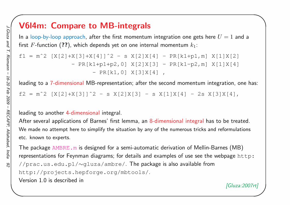
V6l4m: Compare to MB-integralsIn a loop-by-loop approach, after the first momentum integration one gets here U = 1 and a
first F -function (??), which depends yet on one internal momentum k1:
f1 = mˆ2 [X[2]+X[3]+X[4]]ˆ2 - s X[2]X[4] - PR[k1+p1,m] X[1]X [2]
- PR[k1+p1+p2,0] X[2]X[3] - PR[k1-p2,m] X[1]X[4]
- PR[k1,0] X[3]X[4] ,
leading to a 7-dimensional MB-representation; after the second momentum integration, one has:
f2 = mˆ2 [X[2]+X[3]]ˆ2 - s X[2]X[3] - s X[1]X[4] - 2s X[3]X[4],
leading to another 4-dimensional integral.
After several applications of Barnes’ first lemma, an 8-dimensional integral has to be treated.
We made no attempt here to simplify the situation by any of the numerous tricks and reformulations
etc. known to experts.
The package AMBRE.mis designed for a semi-automatic derivation of Mellin-Barnes (MB)
representations for Feynman diagrams; for details and examples of use see the webpage http:
//prac.us.edu.pl/ ∼gluza/ambre/ . The package is also available from
http://projects.hepforge.org/mbtools/ .
Version 1.0 is described in[Gluza:2007rt]
J.G
luza
and
T.Rie
mann
–16-2
0Feb
2009
–RECAPP,Alla
habad,In
dia
92

'&
$%
, the last released version is 1.2. We are releasing now version 2.0, which allows to construct
MB-representations for two-loop tensor integrals.
The package is yet restricted to the so-called loop-by-loop approach, which yields compact
representations, but is known to potentially fail for non-planar topologies with several scales. An
instructive example has been discussed in[Czakon:2007wk]
.
For one-scale problems, one may safely apply AMBRE.mto non-planar diagrams. For our
example V6l4m1 , one gets e.g. with the 8-dimensional MB-representation scetched above the
following numerical output after running also MB.m[Czakon:2005rk]
(see also the webpage http://projects.
hepforge.org/mbtools/ ),
at s = −11:
V6l4m (−s)2ǫ = −0.0522082 1
ǫ− 0.17002 + 0.25606 ǫ + 4.67 ǫ2 + O(ǫ3). (13)
J.G
luza
and
T.Rie
mann
–16-2
0Feb
2009
–RECAPP,Alla
habad,In
dia
93

'&
$%
Compare this to an MB-integral for V6l0mWas solved first in
[Gonsalves:1983nq]
fupc1 = mˆ2 FX[X[3] + X[4]]ˆ2 - PR[k1 + p1, 0] X[1] X[2] -
PR[k1 + p1 + p2, m] X[2] X[3] - PR[k1 - p2, m] X[1] X[4] -
S X[2] X[4] - PR[k1, 0] X[3] X[4]
fupc2 = -s X[2] X[3]-s X[1] X[4]-2 s X[3] X[4]
The function is a scale factor times a pure number
V 6l0m = const(−s)−2−2ǫ
[
A4
ǫ4+
A3
ǫ3+
A2
ǫ2+
A1
ǫ+ A0 + . . .
]
V6l0m = (-s)ˆ-2 - 2 eps
*Gamma[-z1] Gamma[-1 - eps - z1 - z2] Gamma[
1 + z1 + z3] Gamma[-1 - eps - z1 - z3 - z4] Gamma[-z4] Gamma[
1 + z1 + z2 + z4] Gamma[
2 + eps + z1 + z2 + z3 + z4] Gamma[-2 - 2 eps - z2 - z4 -
z5] Gamma[-z5] Gamma[
1 - z1 + z5] Gamma[-2 - 2 eps - z3 - z4 - z6] Gamma[-z6] Gamma[
J.G
luza
and
T.Rie
mann
–16-2
0Feb
2009
–RECAPP,Alla
habad,In
dia
94

'&
$%
3 + eps + z1 + z2 + z3 + z4 + z6] Gamma[
2 + 2 eps + z4 + z5 + z6])/(Gamma[-2 eps] Gamma[
1 - z1] Gamma[-3 eps - z4] Gamma[3 + eps + z1 + z2 + z3 + z4])
integrals = MBcontinue[(-s)ˆ(2 + 2 eps) fin, eps -> 0, rules] ;
26 integral(s) found
J.G
luza
and
T.Rie
mann
–16-2
0Feb
2009
–RECAPP,Alla
habad,In
dia
95

'&
$%
From 1/ǫ4 until ǫ0: at most 4-dimensional
AMBRE output:
-47.8911 + 1/epsˆ4 - 9.8696/epsˆ2 - 33.2569/eps
1
0
-9.869604401660688 -> -Piˆ2
-33.25689147976733 -> -(83/3 * Zeta[3])
-47.89108304541082 -> (-59 Piˆ4/120)
Try PSQL for a systematic study
J.G
luza
and
T.Rie
mann
–16-2
0Feb
2009
–RECAPP,Alla
habad,In
dia
96

'&
$%
Tensor integrals
At the LHC, we need also massive 5-point and 6-point functions at least, for NLO corrections.
In general, the treatment of tensor integrals is a non-trivial task.
• One might think that all tensor numerators may be reduced to (even simpler) scalar
integrands. Important notice: For L > 1, this is not true, we have irreducible numerators,
see next slide.
• For many problems, it i preferrable to evaluate the tensors without knowing the scalar
products. The reasons are different.
J.G
luza
and
T.Rie
mann
–16-2
0Feb
2009
–RECAPP,Alla
habad,In
dia
97

'&
$%
Simple tensor integrals
Bµ ≡ pµ1 B1 =
1
(iπd/2)
∫
ddk kµ
D1D2
Bµν ≡ pµ1pν
1B22 + gµνB20 =1
(iπd/2)
∫
ddk kµkν
D1D2
and B1 and B22, B20 have to be determined.
J.G
luza
and
T.Rie
mann
–16-2
0Feb
2009
–RECAPP,Alla
habad,In
dia
98

'&
$%
Reducible numeratorsSome numerators are reducible – one may divide them out against the denominators:
2kp1
D1 [(k + p1)2 − m22] . . . DN
≡ [(k + p1)2 − m2
2] − [k2 − m21] + (−m2
1 + m22 − p2
1)]
D1[(k + p1)2 − m22] . . .DN
=1
D1D3 . . .DN− 1
D2D3 . . .DN+
−m21 + m2
2 − p21
D1D2D3 . . .DN
This way one derives:
pµ1Bµ = p2B1 =
1
(iπd/2)
∫
ddkp1k
D1D2
=1
(iπd/2)
1
2
∫
ddk
[
1
D1− 1
D2+
−m21 + m2
2 − p21
D1D2
]
and finally:
B1 =1
2p21
[
A0(m1) − A0(m2) + (−m21 + m2
2 − p21)B0(m1, m2, p
2)]
Known to everybody: The Passarino-Veltman reduction scheme for 1-loop tensors
worked out in[Passarino:1979jh]
until 4-point functions.
J.G
luza
and
T.Rie
mann
–16-2
0Feb
2009
–RECAPP,Alla
habad,In
dia
99

'&
$%
Irreducible numeratorsFor a two-loop QED box diagram, it is e.g. L = 2, E = 4, and we have as potential
simplest numerators:
k21, k
22, k1k2 and 2(E − 1) products k1pe, k2pe
compared to N internal lines, N = 5, 6, 7. This gives
I = L + L(L − 1)/2 + L(E − 1) − N irreducible numerators
of this type. Here:
I(N) = 9 − N = 4, 3, 2
This observation is of practical importance:
Imagine you search for potential masters. Then you may take into the list of masters at
most (here e.g.) I(5) = 4, or I(6) = 3, or I(7) = 2 such integrals.
Which momenta combinations are irreducible is dependent on the choice of momenta
flows.
Message:
When evaluating all Feynman integrals by Mellin-Barnes-integrals, one should also learn
to handle numerator integrals
. . . and it is - in some cases - not too complicated compared to scalar ones
The one-loop case: L = 1, E = N , so
I(N) = 1 + (E − 1) − N = 0
irreducible numerators
J.G
luza
and
T.Rie
mann
–16-2
0Feb
2009
–RECAPP,Alla
habad,In
dia
100

'&
$%
The vector integral differs by some numerator kipe and thus there is a single shift in the integrand
k → k + U(x)−1MQ
theR
ddk k/(k2 + µ2) → 0, and no further changes:
G(k1α) = (−1)NνΓ`
Nν −d2L´
Γ(ν1) . . . Γ(νN )
Z 1
0
NY
j=1
dxj xνj−1
j δ
1 −
NX
i=1
xi
!
U(x)Nν−d(L+1)/2−1
F (x)Nν−dL/2
"
X
l
M1lQl
#
α
,
Here also a tensor integral:
G(k1αk2β) = (−1)Nν
Γ`
Nν − d2 L´
Γ(ν1) . . . Γ(νN )
Z 1
0
NY
j=1
dxj xνj−1
j δ
1 −
NX
i=1
xi
!
U(x)Nν−2−d(L+1)/2
F (x)Nν−dL/2
×X
l
"
[M1lQl]α[M2lQl]β −Γ`
Nν − d2 L − 1
´
Γ`
Nν − d2 L´
gαβ
2U(x)F (x)
(V −11l )+(V −1
2l )
αl
#
.
The 1-loop case will be used in the following L times for a sequential treatment of an L-loop
integral (remember∑
xjDj = k2 − 2Qk + J and F (x) = Q2 − J):
G([1, kpe]) = (−1)NνΓ(
Nν − d2
)
Γ(ν1) . . .Γ(νN )
∫ 1
0
N∏
j=1
dxj xνj−1j δ
(
1 −N∑
i=1
xi
)
[1, Qpe]
F (x)Nν−d/2
J.G
luza
and
T.Rie
mann
–16-2
0Feb
2009
–RECAPP,Alla
habad,In
dia
101

'&
$%
.Another nice box with numerator, B5l3m(pe.k1)
We used it for the determination if the small mass expansion.
B5l3m(pe · k1) =m4ǫ(−1)a12345 e2ǫγE
Q5j=1 Γ[ai]Γ[5 − 2ǫ − a123](2πi)4
Z
+i∞
−i∞
dα
Z
+i∞
−i∞
dβ
Z
+i∞
−i∞
dγ
Z
+i∞
−i∞
dδ
(−s)(4−2 ǫ)−a12345−α−β−δ
(−t)δ
Γ[−4 + 2 ǫ + a12345 + α + β + δ]
Γ[6 − 3 ǫ − a12345 − α]
Γ[−α] Γ[−β]
Γ[7 − 3 ǫ − a12345 − α] Γ[5 − 2 ǫ − a123]
Γ[−δ]
Γ[4 − 2 ǫ − a1123 − 2 α − γ] Γ[5 − 2 ǫ − a1123 − 2 α
Γ[2 − ǫ − a13 − α − γ]
Γ[8 − 4 ǫ − a112233445 − 2 α − 2 β − 2 δ − γ]
Γ[4 − 2 ǫ − a12345 − α − β − δ − γ]
Γ[9 − 4 ǫ − a112233445 − 2 α − 2 β − 2 δ − γ]
(pe · p3) Γ[1 + a4 + δ] Γ[6 − 3 ǫ −
Γ[4 − 2 ǫ − a1234 − α − β − δ] Γ[3 − ǫ − a12 − α] Γ[8 − 4 ǫ − a112233445 − 2 α − 2 δ − γ]Γ[9 − 4 ǫ − a112233445 − 2 α − 2 β − 2
Γ[5 − 2 ǫ − a1123 − γ] Γ[4 − 2 ǫ − a1123 − 2 α − γ] Γ[a1 + γ] Γ[−2 + ǫ + a123 + α + δ + γ] + Γ[a4 + δ]
»
−(pe · p1) Γ[7 − 3 ǫ − a
Γ[4 − 2 ǫ − a1234 − α − β − δ]Γ[8 − 4 ǫ − a112233445 − 2 α − 2 δ − γ]Γ[9 − 4 ǫ − a112233445 − 2 α − 2 β − 2 δ − γ]»
Γ[3 − ǫ − a12 − α] Γ[5 − 2 ǫ − a1123 − γ]Γ[4 − 2 ǫ − a1123 − 2 α − γ] Γ[a1 + γ] + Γ[2 − ǫ − a12 − α] Γ[4 − 2 ǫ − a1123 − γ]
Γ[5 − 2 ǫ − a1123 − 2 α − γ] Γ[1 + a1 + γ]
–
Γ[−2 + ǫ + a123 + α + δ + γ] + Γ[6 − 3 ǫ − a12345 − α] Γ[3 − ǫ − a12 − α]
Γ[5 − 2 ǫ − a1123 − γ] Γ[4 − 2 ǫ − a1123 − 2 α − γ]Γ[a1 + γ]
»
((pe · (p1 + p2)) Γ[5 − 2 ǫ − a1234 − α − β − δ]Γ[9 − 4 ǫ − a112233445
Γ[8 − 4 ǫ − a112233445 − 2 α − 2 β − 2 δ − γ]Γ[−2 + ǫ + a123 + α + δ + γ] + (pe · p1) Γ[4 − 2 ǫ − a1234 − α − β − δ]
Γ[8 − 4 ǫ − a112233445 − 2 α − 2 δ − γ]Γ[9 − 4 ǫ − a112233445 − 2 α − 2 β − 2 δ − γ]Γ[−1 + ǫ + a123 + α + δ + γ]
–ff
J.G
luza
and
T.Rie
mann
–16-2
0Feb
2009
–RECAPP,Alla
habad,In
dia
102

'&
$%
Interlude: Tensor integrals, a bit backgroundIntroducing α parameter representations for the propagators,
1
(k2 − m2 + iǫ)ν=
i−ν
Γ(ν)
∫ ∞
0
dααν−1 exp iα(k2 − m2 + iǫ)
one may write e.g. for the L-loop integral with I internal lines and E external lines
G(d) ≡∫
ddk1 . . . ddkL
cν11 . . . cνI
I
exp i(a1k1 + . . . + aLkL)
= i2(π
i
)dL/2 I∏
i=1
i−νi
Γ(ν)
∫ ∞
0
dαiανi−1i
[D(α)]d/2
exp i
[
Q(α, a1, . . . aL)
D(α)−
I∑
i=1
αi(m2i − iǫ)
]
,
with the following notations:
ci = q2i − m2
i + iǫ,
qµi =
L∑
l=1
ωilkµl +
E∑
e=1
ηiepµe =
L∑
l=1
ωilkµl + eµ
i , i = 1, . . . I,
and the ωil and ηie are equal to +1,−1, 0, depending on the topology and on the
distribution of internal momenta. They are incidence matrices of a diagram.
This formula represents a scalar integral for al = 0, and for ai 6= 0 it is an auxiliary
representation for the treatment of tensor integrals.
J.G
luza
and
T.Rie
mann
–16-2
0Feb
2009
–RECAPP,Alla
habad,In
dia
103

'&
$%
The Q and D forms may be determined to be as follows for the 1-loop case:
D = A,
Q(α, a) = DF −(a
2+ E
)2
,
with
A =I∑
i=1
ω2i αi,
Eµ =I∑
i=1
ωieµi αi,
F =I∑
i=1
(eµi )
2αi.
Explicit expressions are given for D and the a-dependent part of Q for the convention
used in Figure ??. We may add the a-independent part Q(a = 0) of the Q form here:
D =∑
αj ,
Q = aµ
∑
αjpµj − 1
4a2 + Q(a = 0),
Q(a = 0) = DF − E2 =(
∑
αj
)(
∑
αkp2k
)
−(
∑
αkpk
)2
.
J.G
luza
and
T.Rie
mann
–16-2
0Feb
2009
–RECAPP,Alla
habad,In
dia
104

'&
$%
The Q and D forms may be determined to be as follows for the 2-loop case
D = A1A2 − M2,
Q(α, a1, a2) = DF − A2E21 − A1E
22 + 2ME1E2 + Q(a1, a2),
and
A1 =I∑
i=1
ω2i1 αi,
A2 =I∑
i=1
ω2i2 αi,
M =
I∑
i=1
ωi1ωi2 αi,
Eµl =
I∑
i=1
ωileµi αi,
F =I∑
i=1
(eµi )
2αi.
The Q(a1, a2) is given in Section ??.
J.G
luza
and
T.Rie
mann
–16-2
0Feb
2009
–RECAPP,Alla
habad,In
dia
105

'&
$%
General tensor reduction to scalars, L = 1The idea for 1-loop integrals and generalization to n-loops; I follow Tausk et al.
[Davydychev:1991va,Tarasov:1996br,Tarasov:1997kx]
J (N)µ1...µR
(d; ν1, . . . , νN ) =
∫
ddk
iπd/2
kµ1. . . kµR
Dν11 . . .DνN
N
= (−1)R
∑
λ,κ1,...,κN
(−1
2)λ
[g]λ[q1]κ1 . . . [qN ]κN
µ1...µR(ν1)κ1
. . . (νN )κN
J (N) (d + 2(R − λ); ν1 + κ1, . . . , νN + κN )
where (ν)κ = Γ(ν+κ)Γ(ν) are Pochhammer symbols and the sum runs over non-negative
integers such that 2λ + κ1 + . . . + κN = R. The next step is to use recurrence relations
to reduce the scalar coefficients J (N) appearing in the decomposition to a set of master
integrals.
It is useful to introduce a notation for certain determinants that occur in the recurrence
relations and their solutions. First, the determinant of an (N + 1) × (N + 1) matrix,
known as the modified Cayley determinant[Melrose:1965kb]
J.G
luza
and
T.Rie
mann
–16-2
0Feb
2009
–RECAPP,Alla
habad,In
dia
106

'&
$%
,
()N ≡
∣
∣
∣
∣
∣
∣
∣
∣
∣
∣
∣
∣
∣
∣
0 1 1 . . . 1
1 Y11 Y12 . . . Y1N
1 Y12 Y22 . . . Y2N
......
.... . .
...
1 Y1N Y2N . . . YNN
∣
∣
∣
∣
∣
∣
∣
∣
∣
∣
∣
∣
∣
∣
, (14)
with coefficients
Yij = −(qi − qj)2 + m2
i + m2j , (i, j = 1 . . .N) . (15)
Although the masses of the propagators appear in the coefficients Yij, the determinant
()N does not depend on them and it is actually proportional to the Gram determinant
of the external momenta of the N -point function in eq. (14). All other determinants we
need are signed minors of ()N , constructed by deleting m rows and m columns from
()N , and multiplying with a sign factor. They will be denoted by
j1 j2 · · · jm
k1 k2 · · · km
N
≡ (−1)P
l(jl+kl)
sgnj sgnk
∣
∣
∣
∣
∣
∣
rows j1 · · · jm deleted
columns k1 · · · km deleted
∣
∣
∣
∣
∣
∣
, (16)
J.G
luza
and
T.Rie
mann
–16-2
0Feb
2009
–RECAPP,Alla
habad,In
dia
107

'&
$%
where sgnj and sgnk are the signs of permutations that sort the deleted rows
j1 · · · jm and columns k1 · · · km into ascending order.
Combining integration by parts identities with relations connecting integrals in different
space-time dimensions[Tarasov:1996br]
, one obtains the following basic recurrence relations[Fleischer:1999hq]
:
()N νjj+J (N)(d + 2) =
[
−(
j
0
)
N
+
n∑
k=1
(
j
k
)
N
k−
]
J (N)(d) ,
(d −n∑
i=1
νi + 1) ()N J (N)(d + 2) =
[
(
0
0
)
N
−n∑
k=1
(
0
k
)
N
k−
]
J (N)(d) ,
(
0
0
)
N
νjj+J (N)(d) =
n∑
k=1
(
0j
0k
)
N
[
d −n∑
i=1
νi(k−i+ + 1)
]
J (N)(d) .
where the operator j± acts by shifting the index νj by ±1.
J.G
luza
and
T.Rie
mann
–16-2
0Feb
2009
–RECAPP,Alla
habad,In
dia
108

'&
$%
Recurrence relations: An application1
d−4 = − 12ǫ
C0(m, 0, m; m2, m2, s) =1
s − 4m2
[
d − 2
d − 4
A0(m2)
m2+
2d − 3
d − 4B0(m, m; s)
]
V 3l2m =−1
s − 4
[
1 − ǫ
ǫT1l1m +
5 − 4ǫ
2ǫSE2l2m
]
(17)
This relates UV-divergent quantities with one which is IR-divergent!
Derivation:
I do not know a simple one.
With use of recurrence relations published in[Tarasov:1996br,Fleischer:1999hq]
it may be done. See[Fleischer:2006ht]
.
Because the am determinant vanishes,(
00
)
3= 0, one of the recurrence relations
J.G
luza
and
T.Rie
mann
–16-2
0Feb
2009
–RECAPP,Alla
habad,In
dia
109

'&
$%
expresses the vertex by a self-energy with 2 massive lines in d − 2 dimensions:
(d − 4) ()3 I(d)3 =
[
(
0
0
)
3
−3∑
k=1
(
0
k
)
3
k−
]
I(d−2)3 = I
(d−2)2 (m, m)
The dimension of the 2-point function may be raised by another recurrence relation,
but now one line will be dotted:
I(d−2)2 (m, m) = −21+Id
2 (m, m), (18)
The dot may be removed, in general form, by expressing a dotted function by itself, butundotted, plus extra terms with one line less, but a dotted one:
„0
0
«
21+
I(d)2
=
"
(3 − d)
„0
1
«
2
#
I(d)2
−
2X
i,k i6=k
„01
0k
«
2k−
i+
I(d)2
, (19)
Here the latter is a dotted tadpole, and that is proportional to the tadpole itself, and
we get the relation needed. (In general, iterations do the job here.)
Direct evaluation shows:
A0(m)dot =1
2(d − 2)
A0(m)
m2
J.G
luza
and
T.Rie
mann
–16-2
0Feb
2009
–RECAPP,Alla
habad,In
dia
110

'&
$%
• hexagon package in Mathematica and (yet) unpublished Fortran code
The packages evaluate
• 6-point functions up to tensor rank 4
• 5-point functions up to tensor rank 3
6-point functions up to tensor rank 4[Fleischer:1999hq,Diakonidis:0901.4455,Diakonidis:2008ij]
J.G
luza
and
T.Rie
mann
–16-2
0Feb
2009
–RECAPP,Alla
habad,In
dia
111

'&
$%
One reduction: 5-point tensor, rank three
Iµ ν λ5 =
4∑
i,j,k=1
qµi qν
j qλkEijk +
4∑
k=1
g[µνqλ]k E00k ,
where
g[µνqλ]k = gµν qλ
k + gµλ qνk + gνλ qµ
k , (20)
with scalar coefficients defined by
Eijk =5∑
s=1
S4,sijkIs
4
+5∑
s,t=1
S3,stijk Ist
3 +5∑
s,t,u=1
S2,stuijk Istu
2 , (21)
J.G
luza
and
T.Rie
mann
–16-2
0Feb
2009
–RECAPP,Alla
habad,In
dia
112

'&
$%
with
S4,sijk =
1
3(
00
)
5
(
ss
)2
5
×
−(
0s
0k
)
5
[(
0s
is
)
5
(
0s
js
)
5
+
(
is
js
)
5
(
0s
0s
)
5
]
+
(
0s
0s
)
5
[(
0i
sk
)
5
(
0s
js
)
5
+
(
0j
sk
)
5
(
0s
is
)
5
]
+ (i ↔ k) + (j ↔ k) , (22)
S3,stijk =
1
3(
00
)
5
(
ss
)2
5
(
0s
0k
)
5
[(
ts
is
)
5
(
0s
js
)
5
+
(
is
js
)
5
(
ts
0s
)
5
+
(
ss
)
5
(
0stist
)
5(
stst
)
5
(
ts
js
)
5
]
−[(
0i
sk
)
5
(
0s
js
)
5
+
(
0j
sk
)
5
(
0s
is
)
5
](
ts
0s
)
5
−[(
0i
sk
)
5
(
ts
js
)
5
+
(
0j
sk
)
5
(
ts
is
)
5
]
×(
ss
)
5
(
0st0st
)
5
2(
stst
)
5
+ (i ↔ k) + (j ↔ k) , (23)
J.G
luza
and
T.Rie
mann
–16-2
0Feb
2009
–RECAPP,Alla
habad,In
dia
113
'&
$%
S2,stuijk = − 1
3(
00
)
5
(
ss
)
5
(
stst
)
5
×(
0s
0k
)
5
(
ts
js
)
5
(
ust
ist
)
5
− 1
2
[(
0j
sk
)
5
(
ust
ist
)
5
+
(
0i
sk
)
5
(
ust
jst
)
5
](
ts
0s
)
5
+ (i ↔ k) + (j ↔ k) , (24)
J.G
luza
and
T.Rie
mann
–16-2
0Feb
2009
–RECAPP,Alla
habad,In
dia
114

'&
$%
and
E00j =1
6(
00
)
5
−5∑
s=1
1(
ss
)2
5
×[
3
(
s
0
)
5
(
0s
js
)
5
−(
s
j
)
5
(
0s
0s
)
5
](
0s
0s
)
5
Is4
+
5∑
s,t=1
1(
ss
)2
5
×[
3
(
s
0
)
5
(
0s
js
)
5
−(
s
j
)
5
(
ts0s
)2
5(
stst
)
5
]
(
ts
0s
)
5
Ist3
−5∑
s,t,u=1
(
s
j
)
5
(
ust0st
)
5(
ss
)
5
(
stst
)
5
(
ts
0s
)
5
Istu2
. (25)
The decomposition in eq. (20) is equivalent to the one found in ref.[Denner:2002ii]
, where the coefficients Eijk and E00j are expressed in terms of tensor 4-point functions. Here,
instead, they are completely reduced to a basis of scalar master integrals consisting of boxes Is4 ,
vertices Ist3 , and 2-point functions Istu
2 obtained by removing lines s, s and t, or s, t and u from
the pentagon.
J.G
luza
and
T.Rie
mann
–16-2
0Feb
2009
–RECAPP,Alla
habad,In
dia
115

'&
$%
Summary
• We have introduced to the representation of L-loop N -point Feynman integrals of general
type
• The determination of the ǫ-poles is generally solved
• The remaining problem is the evaluation of the multi-dimensional, finite MB-Integrals
• This is unsolved in the general case, . . . so you have something to do if you like to . . .
Problem: Determine the small mass limit of B5l2m2 or of any other of the 2-loop boxes for
Bhabha scattering.
Prof. Gluza may check your solution.
He leaves soon.
J.G
luza
and
T.Rie
mann
–16-2
0Feb
2009
–RECAPP,Alla
habad,In
dia
116

'&
$%
On-shell example: B4l2m , the 1-loop on-shell box
den = (x4 d4 + x5 d5 + x6 d6 + x7 d7 // Expand) /. kinBha /. mˆ2 -> 1 // Expand
Q = -Coefficient[den, k]/2 // Simplify
= p3 x4 + p2 x5 - p1 (x4 + x6)
M = Coefficient[den, kˆ2] // Simplify
= x4 + x5 + x6 + x7 -> 1
J = den /. k -> 0 // Simplify
= t x4
F[x] = (Qˆ2 - J M // Expand) /. kinBha /. mˆ2 -> 1 /. u -> -s - t + 4 // E xpand
= (x5+x6)ˆ2 + (-s)x5x6 + (-t)x4x7
B4l2ma = mb[(x5+x6)ˆ2, -tx7x4 - sx5x6, nu, ga]
B4l2mb = B4l2ma /. (-sx5x6 - tx4x7)ˆ(-ga - nu) ->
mb[(-s)x5x6, (-t)x7x4, nu+ga, de]
/.((-s)x5x6)ˆde_ -> (-s)ˆde x5ˆde x6ˆde
/.((x56ˆ2)ˆga -> (x5 + x6)ˆ(2ga)
J.G
luza
and
T.Rie
mann
–16-2
0Feb
2009
–RECAPP,Alla
habad,In
dia
117

'&
$%
=
(inv2piIˆ2(-s)ˆde x5ˆde x6ˆde ((x5 + x6)ˆ(2ga)((-t)x4x7) ˆ(-de-ga-nu)
Gamma[-de] Gamma[-ga] Gamma[de + ga + nu] /Gamma[nu]
B4l2mc = B4l2mb /. (x5 + x6)ˆ(2ga) ->
mb[x5, x6, -2ga, si]
/. ((-t)x4x7)ˆsi_ -> (-t)ˆsi x4ˆsi x7ˆsi // ExpandAll
=
1/(Gamma[-2ga] Gamma[nu])
inv2piIˆ3 (-s)ˆde (-t)ˆ(-de - ga - nu)
x4ˆ(-de - ga - nu) x5ˆ(de + si) x6ˆ(de + 2 ga - si) x7ˆ(-de - ga - nu )
Gamma[-de] Gamma[-ga] Gamma[ de + ga + nu] Gamma[-si] Gamma[ -2ga + si]
B4l2md = xfactor4[a4, x4, a5, x5, a6, x6, a7, x7] B4l2mc
=
.... (-s)ˆde (-t)ˆ(-de-ga-nu)
x4ˆ(-1+a4-de-ga-nu) x5ˆ(-1+a5+de+si) x6ˆ(-1+a6+de+2ga -si) x7ˆ(-1+a7- de-ga-nu)
B4l2me =
B4l2md /.
x4ˆB4_ x5ˆB5_ x6ˆB6_ x7ˆB7_ -> xint4[x4ˆB4 x5ˆB5 x6ˆB6 x7ˆB 7]
= ...
J.G
luza
and
T.Rie
mann
–16-2
0Feb
2009
–RECAPP,Alla
habad,In
dia
118

'&
$%
B4l2mf = B4l2me /.
Gamma[a6 + de + 2 ga - si]Gamma[-si]Gamma[ a5 + de + si] Gamma[- 2 ga + si]
-> barne1[si, a5 + de, -2 ga, a6 + de + 2 ga, 0]
This finishes the evaluation of the MB-representation for B4l2m .
J.G
luza
and
T.Rie
mann
–16-2
0Feb
2009
–RECAPP,Alla
habad,In
dia
119

'
&
$
%Pac
kage:
AM
BRE.m
(K.K
ajda,
with
suppor
tby
J.G
luza
and
TR)
J.Gluza and T. Riemann – 16-20 Feb 2009 – RECAPP, Allahabad, India 120

'&
$%
Example beyond Harmonic Polylogs: QED Box B4l2m[Fleischer:2006ht]
F[x] = (x5+x6)ˆ2 + (-s)x5x6 + (-t)x4x7
B4l2m , the 1-loop QED box, with two photons in the s-channel; the Mellin-Barnes
representation reads for finite ǫ:
B4l2m = Box(t, s) =eǫγE
Γ[−2ǫ](−t)(2+ǫ)
1
(2πi)2
∫ +i∞
−i∞
dz1
∫ +i∞
−i∞
dz2 (26)
(−s)z1(m2)z2
(−t)z1+z2Γ[2 + ǫ + z1 + z2]Γ
2[1 + z1]Γ[−z1]Γ[−z2]
Γ2[−1 − ǫ − z1 − z2]Γ[−2 − 2ǫ − 2z1]
Γ[−2 − 2ǫ − 2z1 − 2z2]
Mathematica package MBused for analytical expansion ǫ → 0:[Czakon:2005rk]
J.G
luza
and
T.Rie
mann
–16-2
0Feb
2009
–RECAPP,Alla
habad,In
dia
121

'&
$%
B4l2m = −1
ǫJ1 + ln(−s)J1 + ǫ
„
1
2
ˆ
ζ(2) − ln2(−s)˜
J1 − 2J2
«
. (27)
with J1 being also the divergent part of the vertex function C0(t;m, 0, m)/s = V3l2m/s (as is
well-known):
J1 =eǫγE
st
1
2πi
Z
−12+i∞
−12−i∞
dz1
„
m2
−t
«z1 Γ3[−z1]Γ[1 + z1]
Γ[−2z1]=
1
m2s
2y
1 − y2ln(y) (28)
with
y =
p
1 − 4m2/t − 1)
(p
1 − 4m2/t + 1)
The J2 is more complicated:
J2 =eǫγE
t21
(2πi)2
Z
−34+i∞
−34−i∞
dz1
“s
t
”z1
Γ[−z1]Γ[−2(1 + z1)]Γ2[1 + z1] (29)
×
Z
−12+i∞
−12−i∞
dz2
„
−m2
t
«
z2Γ[−z2]Γ2[−1 − z1 − z2]
Γ[−2(1 + z1 + z2)]Γ[2 + z1 + z2].
J.G
luza
and
T.Rie
mann
–16-2
0Feb
2009
–RECAPP,Alla
habad,In
dia
122

'&
$%
The expansion of B4l2m at small m2 and fixed value of tWith
mt =−m2
t, (30)
r =s
t, (31)
Look, under the integral, at (−m2/t)z2 ,
and close the path to the right.
Seek the residua from the poles of Γ-functions with the smallest powers in m2 and sum the
resulting series.
we have obtained a compact answer for J2 with the additional aid of XSUMMER[Moch:2005uc]
The box contribution of order ǫ in this limit becomes:
B4l2m[t, s, m2; +1] =1
st
4ζ3 − 9ζ2ln(mt) +2
3ln3(mt) + 6ζ2ln(r) − ln2(mt)ln(r) (32)
+1
3ln3(r) − 6ζ2ln(1 + r) + 2ln(−r)ln(r)ln(1 + r) − ln2(r)ln(1 + r)
+2ln(r)Li2(1 + r) + 2Li3(−r)
+ O(mt).
Remark:
The exact Box function is NOT expressible by Harmonic Polylogs, one may introduce a
J.G
luza
and
T.Rie
mann
–16-2
0Feb
2009
–RECAPP,Alla
habad,In
dia
123

'&
$%
generalization of them: Generalized HPLs.
Automatized tools for this might be developed.
A scetch of the small mass expansion may be made as follows.
First the 1-dim. integral J1.
The leading term comes from the first residue:
J1 = Residue[m_tˆz1 Gamma[-z1]ˆ3 Gamma[1 + z1]/Gamma[-2 z1 ], z1, 0]
= 2 Log[m_t]
WE get a logarithmic mass dependence.
The second integral: Start with z2, first residue is:
I2 = Residue[ m_tˆz2 Gamma[-z2] Gamma[-1 - z1 - z2]ˆ2
Gamma[2 + z1 + z2]/Gamma[-2 - 2 z1 - 2 z2], z2, 0]
= −Γ[−1 − z1]2Γ[2 + z1]
Γ[−2 − 2z1]
The residue is independent of m2/t.
J.G
luza
and
T.Rie
mann
–16-2
0Feb
2009
–RECAPP,Alla
habad,In
dia
124

'&
$%
It has to be integrated over z1 yet, together with the terms which were independent of z2:
I2 ∼∫
dz1rz1+1Γ[−z1]Γ[−2 − 2z1]Γ[1 + z1]
2 Γ[−1 − z1]2Γ[2 + z1]
Γ[−2 − 2z1]
Sum over residues, close path to the left:
Residue[z1 = −n] =(−1)nr1−n
2(−1 + n)3[
2 + (−1 + n)2π2 + (−1 + n) ln[r](2 + (−1 + n) ln[r])]
Residue[z1 = −1] =1
6(3π2 ln[r] + ln[r]3)
and finally:
I2 ∼ Residue[z1 = −1] +∞∑
n=2
Residue[z1 = −n]
The sum can be done also withoput using XSUMMER (here at least), e.g.
ln[r]
Infty∑
n=2
(−1)n(2 + π2 − 2nπ2 + n2π2)r1−n
2(−1 + n)3=
1
2
[
π2 ln(1 + 1/r) − 2Li3 (−1/r)]
etc
J.G
luza
and
T.Rie
mann
–16-2
0Feb
2009
–RECAPP,Alla
habad,In
dia
125

'&
$%
Some routines in mathematica which may be used:
( * Barnes’ first lemma: \int d(si) Gamma(si1p+si)Gamma(si2p +si)Gamma(si1m-si)Gamma(si2m-si)
with 1/inv2piI = 2 Pi I * )
barne1[si_, si1p_, si2p_, si1m_, si2m_] :=
1/inv2piI Gamma[si1p + si1m] Gamma[si1p + si2m] Gamma[
si2p + si1m] Gamma[si2p + si2m] /Gamma[si1p + si2p + si1m + si2 m]
( * Mellin-Barnes integral: (A+B)ˆ(-nu) = 1/(2 Pi I) \int d(si) aˆsi bˆ(-nu - si)
Gamma[-si]Gamma[nu+si]/Gamma[nu] * )
mb[a_, b_, nu_, si_]:=inv2piI aˆsi bˆ(-nu-si)Gamma[-si]G amma[nu+si]/Gamma[nu]
( * After the k-integration, the integrand for \int\prod(dxi x iˆ(ai - 1))\delta(1-\sum xi)
will be (L=1 loop) : xfactorn Fˆ(-nu) Q(xi).pe with nu = a1 + .. + an - d/2 * )
xfactor3[a1_, x1_, a2_, x2_, a3_, x3_] :=
I Piˆ(d/2) (-1)ˆ(a1 + a2 + a3) x1ˆ(a1 - 1) x2ˆ(a2 - 1)x3ˆ(a3 - 1) Gamma[
a1 + a2 + a3 - d/2]/(Gamma[a1]Gamma[a2]Gamma[a3])
( * xinti - the i-dimensional x - integration over Feynman param eters /16 06 2005 * )
xint3[x1_ˆ(a1_) x2_ˆ(a2_) x3_ˆ(a3_) ] :=
Gamma[a1 + 1] Gamma[a2 + 1] Gamma[a3 + 1] / Gamma[a1 + a2 + a3 + 3]
J.G
luza
and
T.Rie
mann
–16-2
0Feb
2009
–RECAPP,Alla
habad,In
dia
126

'&
$%
quote also:[Argeri:2007up]
[Smirnov:2008py]
[Ellis:2007qk]
[Binoth:2008uq]
[Diakonidis:2008ij]
[Bogner:2007cr]
[Heinrich:2008si]
[Fleischer:2007ph]
[Diakonidis:2008dt]
References
J.G
luza
and
T.Rie
mann
–16-2
0Feb
2009
–RECAPP,Alla
habad,In
dia
127

'&
$%
Feynman integrals: scalar and tensor integrals, shrinked anddotted ones
Just to mention what kind of integrals may appear:
• diagrams with numerators:
tensors arise from internal fermion lines:∫
ddki · · · Γν(kνi −pν
n)−mn
(ki−pn)2−m2n
· · ·
• diagrams with shrinked and/or with dotted lines: a sample relation see next page
• relations to simpler diagrams may shift the complexity: 1d−4 = − 1
2ǫ
C0(m, 0, m; m2, m2, s) =1
s − 4m2
[
d − 2
d − 4
A0(m2)
m2+
2d − 3
d − 4B0(m, m; s)
]
V 3l2m =−1
s − 4
[
1 − ǫ
ǫT1l1m +
5 − 4ǫ
2ǫSE2l2m
]
(33)
J.G
luza
and
T.Rie
mann
–16-2
0Feb
2009
–RECAPP,Alla
habad,In
dia
128

'&
$%
SE3l2m(a, b, c, d) = −e2ǫΓE
πD
Z
dDk1dDk2 (k1k2)
−d
[(k1 + k2 − p)2 − m2]b [k21]
a [k22 − m2]c
.
SE3l2m = SE3l2m(1, 1, 1, 0)
SE3l2md = SE3l2m(1, 1, 2, 0)
SE3l2mN = SE3l2m(1, 1, 1,−1)
SE3l2md =−(1 + s) + ǫ(2 + s)
s − 4SE3l2m +
2(1 − ǫ)
s − 4
`
T1l1m2 + 3 SE3l2mN
´
,
=1
2ǫ2+
1
2ǫ−
„
1 − ζ2
2+
1 + x
1 − xln(x) +
1 + x2
(1 − x)21
2ln2(x)
«
+ O(ǫ)
SE3l2m SE3l0m
SE5l3mSE3l3m SE3l1m
SE3l2md
Figure 1: The six two-loop 2-point masters of Bhabha scattering.
J.G
luza
and
T.Rie
mann
–16-2
0Feb
2009
–RECAPP,Alla
habad,In
dia
129

'&
$%
More legs, more loops
Seek methods for an (approximated) analytical or numerical evaluation of more involved
diagrams
Remember: UltraViolet (UV) und InfraRed (IR) divergencies appear
Might try:
• same as for simple one-loop: Feynman parameters, direct integration
• use algebraic relations between integrals and find a (minimal) basis of master
integrals – is a preparation of the final evaluation
• derive and solve (system of) differential equations
• derive and solve (system of) difference equations
• do something else for a direct evaluation of single integrals – of all of them or of
the masters only
Into the last category falls what we present here:
Use Feynman parameters and transform the problem
J.G
luza
and
T.Rie
mann
–16-2
0Feb
2009
–RECAPP,Alla
habad,In
dia
130