evaluation of fuel usage factors in highway construction
TRANSCRIPT

EVALUATION OF FUEL USAGE FACTORS IN HIGHWAY
CONSTRUCTION IN OREGON
Final Report
SPR 668


EVALUATION OF FUEL USAGE FACTORS IN HIGHWAY CONSTRUCTION IN OREGON
Final Report
SPR 668
by
Mark Holmgren, M.S.
Kenneth L. Casavant, Ph.D. Eric Jessup, Ph.D.
Washington State University School of Economic Sciences
Pullman, WA 99164-6210
for
Oregon Department of Transportation Research Section
200 Hawthorne Ave. SE, Suite B-240 Salem OR 97301-5192
and
Federal Highway Administration
400 Seventh Street, SW Washington, DC 20590-0003
May 2010


i
Technical Report Documentation Page
1. Report No.
FHWA-OR-RD-10-19
2. Government Accession No.
3. Recipient’s Catalog No.
5. Report Date
May 2010
4. Title and Subtitle
Evaluation Of Fuel Usage Factors In Highway Construction In Oregon 6. Performing Organization Code
7. Author(s)
Mark Holmgren, Kenneth L. Casavant, Ph.D., and Eric L. Jessup, Ph.D. Washington State University School of Economic Sciences Pullman, WA 99164-6210
8. Performing Organization Report No.
10. Work Unit No. (TRAIS)
9. Performing Organization Name and Address
Oregon Department of Transportation Research Section 200 Hawthorne Ave. SE, Suite B-240 Salem, OR 97301-5192
11. Contract or Grant No.
SPR 668
13. Type of Report and Period Covered Final Report
12. Sponsoring Agency Name and Address
Oregon Department of Transportation Research Section and Federal Highway Administration 200 Hawthorne Ave. SE, Suite B-240 400 Seventh Street, SW Salem, OR 97301-5192 Washington, DC 20590-0003
14. Sponsoring Agency Code
15. Supplementary Notes 16. Abstract:
Prices for different construction materials change frequently. In recent years, the price for these different materials has dramatically increased. This result leads contractors to inflate the bid price for a construction project in order to cover the potential increased cost. In an attempt to modify the inflation inserted into bid prices, the Oregon Department of Transportation allows for adjustments in the monthly payment to the contractor for various inputs. One major input that receives an adjustment is fuel. The contractor is eligible to receive adjustments in the monthly payments for fuel when the project is of a certain magnitude. After the project qualifies for the adjustment, when the price of fuel varies by more than twenty-five percent positive or negative from the previous month, the ODOT will make a fuel price adjustment to the monthly payment. The fuel price adjustment is a function of a fuel usage factor. The value for the fuel usage factor for different bid items is based on an over thirty five year old 1974 national survey titled, “Fuel Usage Factors for Highway Construction.” From that original survey the fuel usage factor for each bid item was recommended to be multiplied by the distance, weight, or volume built of the respective bid item, but not for structures. The fuel usage factor for structures was to be multiplied by the gallons of fuel used per $1,000 worth of work. The research presented in this report determines from a national survey whether other states, and their DOTs, use this same procedure to calculate a fuel price adjustment, and if so, whether the values for the fuel usage factors are the same. In addition, the report examines how the price of structural construction has changed over time to ascertain whether the current fuel usage factor for structures is still applicable. A new index is developed in a national model and one for the state of Oregon.
17. Key Words:
Factors, Fuel Factors, Billing, Administration, State Contract Billing, Fuel Price Adjustment, Structures, Bid Items, Trigger Values
18. Distribution Statement
Copies available from NTIS, and online at http://www.oregon.gov/ODOT/TD/TP_RES/
19. Security Classification (of this report)
Unclassified
20. Security Classification (of this page)
Unclassified 21. No. of Pages
113
22. Price
Technical Report Form DOT F 1700.7 (8-72) Reproduction of completed page authorized Printed on recycled paper

SI* (MODERN METRIC) CONVERSION FACTORS
APPROXIMATE CONVERSIONS TO SI UNITS APPROXIMATE CONVERSIONS FROM SI UNITS
Symbol When You Know Multiply By To Find Symbol Symbol When You Know Multiply By To Find Symbol
LENGTH LENGTH
in inches 25.4 millimeters mm mm millimeters 0.039 inches in ft feet 0.305 meters m m meters 3.28 feet ft yd yards 0.914 meters m m meters 1.09 yards yd mi miles 1.61 kilometers km km kilometers 0.621 miles mi
AREA AREA
in2 square inches 645.2 millimeters squared mm2 mm2 millimeters squared 0.0016 square inches in2
ft2 square feet 0.093 meters squared m2 m2 meters squared 10.764 square feet ft2 yd2 square yards 0.836 meters squared m2 m2 meters squared 1.196 square yards yd2 ac acres 0.405 hectares ha ha hectares 2.47 acres ac mi2 square miles 2.59 kilometers squared km2 km2 kilometers squared 0.386 square miles mi2
VOLUME VOLUME fl oz fluid ounces 29.57 milliliters ml ml milliliters 0.034 fluid ounces fl oz gal gallons 3.785 liters L L liters 0.264 gallons gal ft3 cubic feet 0.028 meters cubed m3 m3 meters cubed 35.315 cubic feet ft3 yd3 cubic yards 0.765 meters cubed m3 m3 meters cubed 1.308 cubic yards yd3
NOTE: Volumes greater than 1000 L shall be shown in m3.
MASS MASS oz ounces 28.35 grams g g grams 0.035 ounces oz lb pounds 0.454 kilograms kg kg kilograms 2.205 pounds lb T short tons (2000 lb) 0.907 megagrams Mg Mg megagrams 1.102 short tons (2000 lb) T
TEMPERATURE (exact) TEMPERATURE (exact)
°F Fahrenheit (F-32)/1.8 Celsius °C °C Celsius 1.8C+32 Fahrenheit °F
*SI is the symbol for the International System of Measurement
ii

ACKNOWLEDGEMENTS
This report represents a synthesis of information and data from a variety of sources that significantly improved the final product. Individuals that contributed their time and knowledge include members of the Technical Advisory Committee: Dan Anderson (ODOT), Kevin Brophy (ODOT), Jeff Graham (FHWA), Richard Munford (ODOT), John Riedl (ODOT) and Theresa Yih (ODOT). Special thanks are also extended to Jon Lazarus (ODOT) for his invaluable guidance as technical monitor and to the Research Section at the Oregon Department of Transportation for funding this study.
DISCLAIMER
This document is disseminated under the sponsorship of the Oregon Department of Transportation in the interest of information exchange. The state of Oregon assumes no liability of its contents or use thereof. The contents of this report reflect the views of the authors who are solely responsible for the facts and accuracy of the material presented. The contents do not necessarily reflect the official views of the Oregon Department of Transportation. The state of Oregon does not endorse products of manufacturers. Trademarks or manufacturers’ names appear herein only because they are considered essential to the object of this document. This report does not constitute a standard, specification, or regulation.
iii

iv

EVALUATION OF FUEL USAGE FACTORS IN HIGHWAY CONSTRUCTION IN OREGON
TABLE OF CONTENTS
1.0 BACKGROUND AND SIGNIFICANCE OF WORK ...................................................1
1.1 OBJECTIVES OF THE STUDY .....................................................................................3 1.2 BENEFITS.......................................................................................................................3
2.0 LITERATURE REVIEW .................................................................................................5
2.1 SUPPORTING STUDIES AS GUIDES TO ODOT’S FUTURE STRUCTURE
OF FUEL FACTOR ADJUSTMENTS............................................................................9 2.2 FUEL ADJUSTMENT METHODS IN THE WESTERN STATES AND
FLORIDA ......................................................................................................................11 2.2.1 Arizona.................................................................................................................................................12 2.2.2 Colorado..............................................................................................................................................12 2.2.3 Idaho....................................................................................................................................................14 2.2.4 Montana...............................................................................................................................................15 2.2.5 Nevada .................................................................................................................................................16 2.2.6 Utah .....................................................................................................................................................17 2.2.7 Washington ..........................................................................................................................................19 2.2.8 Wyoming ..............................................................................................................................................20 2.2.9 Florida .................................................................................................................................................21
2.3 SUMMARY...................................................................................................................23
3.0 A NATIONAL SURVEY.................................................................................................25
3.1 THE IMPLEMENTATION PROCEDURE...................................................................25 3.2 RECENT CHANGES IN THE FUEL ADJUSTMENT.................................................30 3.3 SOURCE OF PRICE INDEX.........................................................................................34 3.4 TRIGGER VALUE........................................................................................................35 3.5 CONTRACTOR’S CONCERNS...................................................................................37 3.6 STATES OPINION ABOUT PRICE ADJUSTMENT PAYMENT..............................37 3.7 NEED FOR CHANGE? .................................................................................................42 3.8 SURVEY OVERVIEW .................................................................................................43 3.9 SURVEY SUMMARY ..................................................................................................43
4.0 INFLATION INDICES ...................................................................................................45
4.1 BACKGROUND ...........................................................................................................45 4.2 REVIEW OF CURRENT INDICES ..............................................................................46 4.3 FORMATION OF BID ITEM LIST ..............................................................................58 4.4 THE NATIONAL PROTOTYPE ..................................................................................60 4.5 OREGON STATE INDEX ............................................................................................67 4.6 ANALYSIS....................................................................................................................74 4.7 RELATIONSHIP OF THE TWO INDICES ..................................................................77 4.8 FORMATION OF TWO ADDITIONAL INDICES......................................................79
v

4.9 SUMMARY OF INDICES ............................................................................................87
5.0 CONCLUSIONS AND RECOMMENDATIONS.........................................................89
6.0 REFERENCES.................................................................................................................91
APPENDICES APPENDIX A: TELEPHONE STATE SURVEY APPENDIX B: HISTORIC UNIT PRICES
LIST OF TABLES
Table 2.1: Oregon Highway Construction for Structures Cost Trend (Base Index: 1987 = 100) .................................5 Table 2.2: ODOT Average Annual Asphalt Cement Material Price .............................................................................6 Table 2.3: ODOT Average Annual Fuel Price History .................................................................................................6 Table 2.4: FHWA Historic Prices for Reinforcing Steel, Structural Steel, and Structural Concrete ............................7 Table 2.5: Oregon Fuel Escalation Project Determination ............................................................................................8 Table 2.6: Fuel Usage Factors for Colorado................................................................................................................13 Table 2.7: Fuel Usage Factors for Idaho .....................................................................................................................15 Table 2.8: Fuel Usage Factors for Nevada ..................................................................................................................17 Table 2.9: Fuel Usage Factors for Utah.......................................................................................................................18 Table 2.10: Washington Contract Duration Factor .....................................................................................................19 Table 2.12: Fuel Usage Factors for Florida.................................................................................................................22 Table 3.1: States’ methods for Fuel Adjustment .........................................................................................................26 Table 3.2: Values for Fuel Usage Factors ...................................................................................................................28 Table 3.3: The Diesel Fuel Price Adjustment Schedule for Alaska ............................................................................29 Table 3.4: States’ Methods for Fuel Adjustments, Recent Changes, and Alternative Methods..................................31 Table 3.5: Sources for the Fuel Index .........................................................................................................................34 Table 3.6: Most Common Trigger Values...................................................................................................................36 Table 3.7: States Responses about Fairness and Risk .................................................................................................38 Table 3.8: Fuel Adjustment Percent of the Annual Total Budget (2008)....................................................................39 Table 3.9: Total Amount Paid in Fuel Adjustments for 2008 .....................................................................................40 Table 3.10: Historic Fuel Price Adjustments...............................................................................................................42 Table 4.1: California Department of Transportation Average Highway Contract Prices............................................46 Table 4.2: Colorado Highway Construction Cost Index .............................................................................................48 Table 4.3: Oregon Highway Construction Cost Trends ..............................................................................................49 Table 4.4: South Dakota Department of Transportation Highway Construction Cost Index......................................51 Table 4.5: Price Trends for Utah Highway Construction ............................................................................................52 Table 4.6: Washington State Department of Transportation Unit Bid Prices..............................................................54 Table 4.7: Price Trends for Federal-Aid Highway Construction Structures (1987 Base) ...........................................56 Table 4.8: Most costly and frequently used structural bid items from 1991 to 2008 ..................................................58 Table 4.9: Bid Item Descriptions from RS Means .......................................................................................................60 Table 4.10: National Bid Item Unit Prices ..................................................................................................................61 Table 4.11: Annual Percentage Cost of Total Structural Construction for Selected Bid Items...................................64 Table 4.12: National Percentage Change in Price for Selected Bid Items...................................................................65 Table 4.13: National Percentage Change in Price Multiplied by Respective Weighted Average ...............................66 Table 4.14: National Prototype....................................................................................................................................66 Table 4.15: Oregon Bid Item Unit Prices ....................................................................................................................67 Table 4.16: Oregon State Percentage Change in Price for Selected Bid Items ...........................................................71 Table 4.17: Oregon State Percentage Change in Price Multiplied by Respective Weighted Average........................72 Table 4.18: Oregon State Index...................................................................................................................................73 Table 4.19: Linear Trend for Each Bid Item ...............................................................................................................79 Table 4.20: Annual Percentage Cost of Oregon’s Total Structural Construction for Selected Bid Items...................80
vi

vii
Table 4.21: FHWA Percentage Change in Price for Selected Bid Items.....................................................................81 Table 4.22: Oregon Percentage Change in Price for Selected Bid Items ....................................................................82 Table 4.23: FHWA Percentage Change in Price Multiplied by Respective Weighted Average .................................83 Table 4.24: Oregon Percentage Change in Price Multiplied by Respective Weighted Average.................................84 Table 4.25: FHWA Index ............................................................................................................................................85 Table 4.26: Adjusted Oregon State Index ...................................................................................................................86
LIST OF FIGURES
Figure 4.1: California’s Historic Reinforcing & Structural Steel Contract Prices ......................................................47 Figure 4.2: California’s Historic Structural Concrete Contract Prices ........................................................................47 Figure 4.3: Colorado’s Historic Reinforcing & Structural Steel Bid Prices................................................................48 Figure 4.4: Colorado’s Historic Structural Concrete Contract Prices .........................................................................49 Figure 4.5: Oregon’s Historic Reinforcing & Structural Steel Bid Prices...................................................................50 Figure 4.6: Oregon’s Historic Structural Concrete Bid Prices ....................................................................................50 Figure 4.7: South Dakota’s Historic Reinforcing & Structural Steel Bid Prices.........................................................51 Figure 4.8: South Dakota’s Historic Structural Concrete Bid Prices ..........................................................................52 Figure 4.9: Utah’s Historic Reinforcing & Structural Steel Bid Prices.......................................................................53 Figure 4.10: Utah’s Historic Structural Concrete Bid Prices.......................................................................................54 Figure 4.11: Washington’s Historic Reinforcing & Structural Steel Bid Prices .........................................................55 Figure 4.12: Washington’s Historic Structural Concrete Bid Prices ...........................................................................55 Figure 4.13: FHWA’s Historic Reinforcing & Structural Steel Contract Prices.........................................................57 Figure 4.14: FHWA’s Historic Structural Concrete Contract Prices...........................................................................57 Figure 4.15: National Historic Structural Excavation Bid Item Unit Prices................................................................62 Figure 4.16: National Historic Reinforcement, Coated Reinforcement, & Structural Steel Bid Item Unit Prices ......62 Figure 4.17: National Historic Structural Concrete Bid Item Unit Prices ...................................................................63 Figure 4.18: National Historic Steel Rail Bid Item Unit Prices...................................................................................63 Figure 4.19: Oregon’s Historic Structural Excavation Bid Item Unit Prices ..............................................................68 Figure 4.20: Oregon’s Historic Reinforcement, Coated Reinforcement, & Structural Steel Bid Item Unit Prices.....69 Figure 4.21: Oregon’s Historic Structural Concrete Bid Item Unit Prices ..................................................................69 Figure 4.22: Oregon’s Historic 2 Tube Steel Rail Bid Item Unit Prices .....................................................................70 Figure 4.23: Price Percentage Change Trend for Structural Excavation.....................................................................74 Figure 4.24: Price Percentage Change Trend for Reinforcement................................................................................75 Figure 4.25: Price Percentage Change Trend for Coated Reinforcement....................................................................75 Figure 4.26: Price Percentage Change Trend for Class 5000 Concrete.......................................................................76 Figure 4.27: Price Percentage Change Trend for Structural Steel...............................................................................76 Figure 4.28: Price Percentage Change Trend for Steel Rail ........................................................................................77 Figure 4.29: Price Percentage Change Trend for the National Prototype and Oregon State Index.............................78 Figure 4.30: Price Percentage Change Trend for the FHWA Index and Adjusted Oregon State Index......................87


1.0 BACKGROUND AND SIGNIFICANCE OF WORK
Price volatility of construction materials and supplies such as asphalt, fuel, cement, and steel can create significant problems for construction contractors when preparing realistic and accurate bids. It can also be problematic for agencies sponsoring the projects. In many cases, the bidder or construction company cannot obtain firm price quotes from material suppliers for the duration of the project. This type of uncertainty can lead to price speculation and inflated bid prices by the contractor to protect against possible price increases.
Although price speculation and bid inflation are not new, escalation of global fuel prices in 2008 led to greater uncertainty in the bidding process. The effects of higher fuel prices are magnified when combined with the other component prices for concrete and asphalt, along with other demand factors currently affecting the construction industry.
Since 1974, the building and construction industry, as well as some state and federal departments of transportation, have handled this problem by allowing specific price adjustments for select commodities in highway contracting. For the contractors, these adjustments decrease the risk of fluctuating prices over the life of a contract. The application of fuel usage factors is generally accepted as a way to obtain bids that more closely reflect actual costs for any given project. More accurate estimates, however, can only be achieved if the fuel factors accurately reflect the fuel consumption.
Fuel usage factors were published in Highway Research Circular Number 1581 by the Highway Research Board in July 1974. Later, in 1980, they were formally incorporated into the Federal Highway Administration (FHWA) publication Technical Advisory T 5080.3. These fuel factors, however, have not been revised in 35 years, despite obvious changes in the purchasing power of construction dollars, construction techniques, industry innovations, and the type of fuel used for the wide-ranging tasks in construction. Because fuel factors have not been brought up to date, the Oregon Department of Transportation (ODOT) has stated that “it is very unlikely that those fuel usage factors are accurate or effective in removing the risk of fuel price fluctuations to the grantor or construction firm.
Under established fuel factors, diesel and gasoline consumption per unit of work are specified for each nonstructural unit of work (excavation, aggregates, asphalt concrete, and portland cement concrete pavement). The process involves applying the quantities of completed work to the fuel factors in the table, summing the total used for each separate item, and applying the
1 The authors conducted an exhaustive search to obtain this original FHWA study upon which so many states have based their fuel factors adjustments. It was determined that this study was originally housed at one of the regional FHWA facilities but when FHWA was re-organized in the mid-1990’s, this report (and any data or documentation related to the study) was lost at that time. Without being able to review the 1974 study or the methods incorporated, the authors of this report have proceeded under the assumption that the study was conducted utilizing the best available information and methods at the time and sound analytical techniques.
1

price adjustments. Gasoline and diesel fuel usage factors exist for excavation (gallons per cubic yard), aggregate and asphalt production and hauling (gallons per ton), and portland cement concrete (PCC) production and hauling (gallons per cubic yard).
Of particular concern, fuel usage factors for structures and miscellaneous construction are expressed in gallons per $1,000 of construction based on 1980 estimates. ODOT’s construction expenditures in recent years have increased from about $250 million per year to $400-500 million per year, mostly for bridge construction. What this amount of capital buys in physical construction compared to earlier years has decreased considerably, resulting in higher fuel allowance for a given physical structure. Dramatic fuel price increases in the summer of 2008, have also contributed to the overall difficulty and price sensitivity regarding vendor reimbursement. Consequently, inflation and construction cost indices are increasingly important areas of research.
ODOT has identified three analytically separable sources of error in the current method:
1. Inflation. The effect of inflation on construction costs over the last three decades is a primary concern for structures and miscellaneous construction. Fuel usage factors were calculated in gallons per $1000 in 1980 and have never been revisited.
2. Construction Practices and Fuel Efficiency. The relationship of fuel consumption to the production and transportation of specified quantities of aggregate asphalt and PCC have likely been affected by changes in construction practices, use of new and prefabricated materials, improved equipment, and improved fuel efficiency on new and old machines.
3. Fuel Preferences. There have been changes in fuel preference, particularly in the substitution of natural gas for diesel in asphalt plant operations.
The research here will focus primarily on the first source of potential error — the effects of inflation on construction costs. General information on the other two sources of error dealing with unit price fuel factors, however, will be generated to some degree. Continuing research efforts through the extension of this current project could address the other factors identified above.
The primary research document on the application of fuel usage factors is The Development and Use of Fuel Price Adjustment Contract Provisions (FHWA 1980). The AASHTO Subcommittee on Construction’s August 2005 survey summarized contract price adjustment clauses used by states for asphalt cement, fuel, steel, and portland cement.
This report directly evaluates the impact of inflation on the applicability of current fuel usage factors in Oregon and the nation. The results provide information and recommendations that all states may consider and many may adopt, given that improvements in usage and application have been found.
2

1.1 OBJECTIVES OF THE STUDY
The overall objective of this study was to determine the impact of inflation, if any, on structural bid items. To meet this objective, the goals of this research project were to:
1. Compile the state’s fuel adjustment methods for structures.
2. Analyze the effects of inflation in relevant areas of structural construction costs.
3. Analyze the current fuel factors for accuracy while updating them to reflect current conditions in various construction materials and processes.
4. Develop a revised fuel usage factor for structures as addressed in the current FHWA Technical Advisory T 5080.3 and the current process for ODOT.
1.2 BENEFITS
Given limited public budgets, reasonable construction costs are critical to providing the quality of services expected from ODOT. The correspondence between estimated fuel usage and actual fuel usage in construction bids, based on the 35 year-old fuel factors, may no longer be accurate. Examining the current structure of these factors in current dollars and the fuel used in construction will allow decisions to be made regarding the need for new fuel factors to mitigate risk, while getting the most construction for the dollar for ODOT. Risk and uncertainty, under extremely volatile construction cost market situations, may result in overpriced bids. A sound basis for associating fuel usage with higher construction is critically important for the responsible allocation of public funds. Additionally, less administrative oversight and effort are required with a more accurate and dynamic adjustment tool. Thus, the payoff potential is very high for Oregon and the nation through the FHWA’s reconsideration of the Technical Advisory T 5080.3. The construction industry will also be better served through minimization of risk in bidding estimates, related to fuel in the construction processes.
3

4

2.0 LITERATURE REVIEW
The research team began by investigating the price of materials for construction projects over the past several years, along with the components that make up the majority of construction bid costs. When prices for different construction materials increase, it becomes difficult for contractors to make an accurate bid.
Fluctuations in fuel prices also directly affect the Oregon Department of Transportation (ODOT). ODOT allows a fuel price adjustment for different projects if they meet certain criteria. Particular bid items in construction are designated with a specific fuel factor. As illustrated below in Table 2.1, the construction cost for structures has increased considerably over the last several years. From 1987 to 2007, highway construction costs for structures in Oregon have increased 163 percent.
Table 2.1: Oregon Highway Construction for Structures Cost Trend (Base Index: 1987 = 100) Year Index Chart 1987 100.0
1988 114.1
1989 118.1
1990 109.9
1991 124.3
1992 104.5
1993 101.0
1994 116.9
1995 136.4
1996 133.4
1997 172.4
1998 157.5
1999 190.2
2000 136.8
2001 123.4
2002 164.1
2003 175.2
2004 159.8
2005 221.8
Source: (ODOT 2007a)
5

ODOT’s asphalt cement material price index and fuel price index (Tables 2.2 and 2.3, respectively) show that prices have increased by more than 70 percent, and 189 percent, respectively, from 2003 to 2007.
Table 2.2: ODOT Average Annual Asphalt Cement Material Price Year Pacific Northwest ($/ton) Boise Idaho ($/ton) 2003 $175.00 $155.00 2004 $181.42 $171.50 2005 $192.25 $192.42 2006 $298.75 $340.25 2007 $327.92 $362.17
Source: (ODOT 2007b)
Table 2.3: ODOT Average Annual Fuel Price History Year Price ($/Gallon) 2003 $0.91 2004 $1.29 2005 $1.82 2006 $2.12 2007 $2.23
Source: (ODOT 2007c) The price of reinforcing steel, structural steel, and structural concrete has increased by more than 32 percent, 26 percent, and 17 percent, respectively, from 2001 to the first quarter of 2006. Table 2.4 shows FHWA reported prices of reinforcing steel, structural steel, and structural concrete from 1972 to 20062 .
2 FHWA discontinued these reports after the first quarter of 2006.
6

Table 2.4: FHWA Historic Prices for Reinforcing Steel, Structural Steel, and Structural Concrete
Year Reinforcing Steel
Avg. Contract Price ($/lb.) Structural Steel
Avg. Contract Price ($/lb.) Structural Concrete
Avg. Contract Price ($/cu. yd.) 1972 0.181 0.342 100.17 1973 0.207 0.372 111.81 1974 0.339 0.551 136.80 1975 0.297 0.554 138.76 1976 0.258 0.484 139.59 1977 0.272 0.520 143.51 1978 0.316 0.603 172.41 1979 0.421 0.759 211.33 1980 0.483 0.941 226.68 1981 0.438 0.790 231.64 1982 0.407 0.762 219.63 1983 0.398 0.708 213.85 1984 0.409 0.709 218.02 1985 0.444 0.796 243.60 1986 0.442 0.850 236.37 1987 0.441 0.885 240.81 1988 0.494 0.924 274.12 1989 0.556 1.018 283.40 1990 0.529 1.010 286.18 1991 0.505 1.030 264.98 1992 0.520 0.916 259.61 1993 0.467 0.861 261.89 1994 0.515 0.847 271.94 1995 0.542 0.922 302.66 1996 0.581 1.068 293.85 1997 0.567 1.186 320.90 1998 0.544 1.111 337.25 1999 0.554 1.224 342.24 2000 0.549 1.351 363.66 2001 0.601 1.201 339.44 2002 0.610 1.436 374.96 2003 0.718 1.219 406.02 2004 0.815 1.521 331.49 2005 0.941 1.571 394.88 2006 0.795 (Q1) 1.520 (Q1) 397.21 (Q1)
Note: FHWA no longer keeps this information after the 1st Quarter (Q1) of 2006. Source: (FHWA 2007) The index for highway construction costs has increased by more than 60 percent within the last five years. The complete list of bid items, and respective fuel factors and minimum qualifiers are shown in Table 2.5
7

Table 2.5: Oregon Fuel Escalation Project Determination
BID ITEM UNIT FUEL FACTOR
($) MIN QUALIFIER
($) General Excavation Yd3 0.29 5,000 Embankment in Place Yd3 0.29 5,000 Subgrade Stabilization (12 in. depth) Yd2 0.33 5,000 Trench Excavation Yd3 0.29 5,000 Stone Embankment Yd3 0.29 5,000 Other Excavation Yd3 0.29 5,000 Cold Plane Removal Yd3 0.72 5,000 Cold Plane Removal Yd2 0.04 5,000 Conc. Pvmt. Diamond Grinding Yd2 0.04 5,000 Base Aggr., Shoulder Aggr. & Sub-Base Aggr. (Combined)
Ton 0.69 5,000
Shoulder Aggregate (Overlays) Ton 0.69 5,000 Cement Treated Base Ton 1.00 5,000 Bituminous Base Ton 2.93 5,000 AC Mixture Ton 2.93 5,000 Aggregate in Chip Seal Ton 0.69 5,000 Emulsified AC Mixture Ton 1.00 5,000 Concrete Pavement Yd2 1.00 5,000 Other PCC: Yd2 1.00 5,000 Structures (Gallons/$1000) Pre-cast 10.00 10,000
Structures (Gallons/$1000) Cast-in-
place 19.00 COMBINED
Total for Project 25,100
Source: (ODOT “unpublished data”) For a bid item to be eligible for a fuel price adjustment, it must first meet a minimum qualifier threshold, which is calculated by multiplying the total quantity of work for each item over the whole project by the respective factor. The sum of eligible bid items has to be greater than 25,100 gallons for the entire project to qualify for a fuel price adjustment. An adjustment will be made through monthly payments for eligible bid items that were used during construction if the price of fuel3 increases or decreases by more than 25 percent. In other words, there will be an increase in payment when fuel prices increase by more than 25 percent and a deduction when fuel prices decrease by more than 25 percent. Section 2.2 presents a review of how other states address fuel price fluctuations and alternative methods for fuel price adjustments.
3 Fuel price is based from the Oil Price Information Service (OPIS).
8

According to the Federal Acquisition Regulation, the U.S. government will not make payment adjustments to a private contractor if the price of construction materials increases during building repair or construction, unless it is written in the contract before the contract is accepted. Furthermore, the responsibility lies with the contractor to write it in the contract, otherwise no additional payments will be made. After viewing various department of transportation (DOT) web sites, most states have some type of fuel price adjustment, and in several states make it optional for the contractor.
In addition to reviewing the literature, the research team examined fuel price adjustment approaches for 10 western states.4 The results indicate there is high variability between the approaches of different states to the adjustment process. Two of the 10 states do not allow for any fuel price adjustment. Some states’ fuel price adjustment requirements are more restrictive than others. For example, in some states any project is eligible for a fuel price adjustment, while in other states project size determines adjustment eligibility. A detailed explanation for each of these 10 states in the western United States and Florida is presented. First, the states that use a fuel price adjustment are identified. Subsequently, specific requirements for fuel price adjustment eligibility are described. Finally, for projects entitled to a fuel price adjustment, the specific bid items included in the fuel price adjustment are listed for each state.
2.1 SUPPORTING STUDIES AS GUIDES TO ODOT’S FUTURE STRUCTURE OF FUEL FACTOR ADJUSTMENTS
In 2006, the American Association of State Highway and Transportation Officials (AASHTO) and Federal Highway Administration (FHWA) jointly prepared a survey to determine the effects of recent price increases and the decline in competition for bids (FHWA 2006a). Forty-four state DOTs responded to the survey. Survey results showed that over a one year period eight states5 implemented or made changes to their fuel price adjustment process. Thirty-one states did not make changes, and California and Maryland reported that they do not have a fuel price adjustment. North Dakota stated they were developing a fuel price adjustment clause. Twenty-two states used a price adjustment clause for certain materials to encourage competition and to compensate for significant cost increases. Arizona and Kentucky reported that using price adjustment clauses has effectively promoted competition and controlled costs.
The Contract Administration Section of the AASHTO Subcommittee on Construction also surveys all states regarding the use of price adjustment clauses. The adjustment clauses for fuel, asphalt cement, steel, and portland cement are analyzed and updated on a regular basis; the most recent survey was administered in the fall of 2008 (AASHTO Subcommittee on Construction, Contract Administration Section 2008). For the fuel price adjustment, the survey reports whether the adjustment exists, the fuel index used, the trigger value, whether the adjustment is optional, the web reference, and additional comments. Contact information is provided for each state.
4 Arizona, California, Colorado, Idaho, Montana, Nevada, New Mexico, Utah, Washington, and Wyoming 5 Colorado, Delaware, Idaho, Kansas, Ohio, South Carolina, Virginia, and Washington
9

In 2004, the Monmouth County Department of Human Services in New Jersey contracted with the Alan M. Voorhees Transportation Center at Rutgers University to identify fuel price indexing/adjustment techniques in the public transportation industry (2004). The purpose of the study was to learn what fuel price adjustments agencies use and outsource to the private sector. The report listed the following four most common fuel price adjustments and the benefits and drawbacks of each method:
1. Contract Pricing. The price for fuel cost reimbursement, based on fuel price fluctuations during the contracting process, is set before the project is started. If prices fluctuate below the contract price then the agency pays more than the market price. Conversely, if prices fluctuate above the set price, providers must absorb the higher price, which could limit the number of firms making a bid on the contract.
2. Fixed Price with Adjustment. If the price of fuel rises by a certain percentage, then the provider receives an additional payment for the increase in fuel price. Since the agency will make additional payments for changes in fuel prices, some of the risk in construction costs is transferred from the provider to the agency. ODOT currently uses this method.
3. Direct Refueling Using Agency-Operated Fueling Facilities. The agency owns its own fleet and refuels them at county owned and operated refueling facilities. The agency has control over the fuel price, but shifts the risk from the provider to the agency.
4. Floating Price. Fuel is treated as a pass-through cost. The provider buys the fuel and the agency reimburses for specific cases. The price risk for the provider is eliminated, but leaves the agency susceptible to dramatic price fluctuations.
The Alan M. Voorhees Transportation Center et al. made the following observations from the survey (2004):
Fuel price changes affect all parties.
Placing the burden of risk on providers will lead to inflated costs and possibly lower quality service.
The fixed price with adjustment method appeared to be favored by the agency and the provider.
Administrative complexity likely burdens both the agency and the provider.
Carroll et al. (2006) performed an extensive literature review and described the methods used for calculating the fuel adjustment by southeastern states including Alabama, Delaware, Florida, Kentucky, Maryland, North Carolina, South Carolina, West Virginia, and West Virginia. They conclude that fuel adjustment policies lead to inefficiency in a firm’s choice of technology.
The FHWA report entitled Technical Advisory T 5080.3 (FHWA 1980) outlines the procedures for development and use of price adjustment contract provisions. According to the FHWA, price adjustments should apply to both upward and downward movements of prices. When an
10

adjustment is implemented into a contract, it should be based on an index from suppliers serving the area. The base index for any item is the price of that item at the beginning of the month in which bids are received. The current index is established on the first business day of each month. When there is a significant difference between the base index and the current index (which is suggested to be between 3 and 10 percent) then an adjustment should be made to the contractor. FHWA suggests calculating this index each month. Additional considerations for fuel adjustments are also noted in the report. For instance, the difference between the base index price and current index price should be multiplied by the appropriate value since fuel is usually considered to be incidental to the project. For non-structural items the value is the quantities of work multiplied by the respective fuel usage factor. For structural items, the value is the fuel consumed per $1,000 of work is multiplied by the respective fuel usage factor. An appendix within Technical Advisory T 5080.3 (FHWA 1980) includes some suggested fuel usage factors. One alternative suggested in the research circular is that the fuel usage factor be calculated as a percent rather than a value. Once each bid item has been multiplied by the respective fuel usage factor, the sum of the values represents the total price adjustment.
The Technical Advisory T 5080.3 (FHWA 1980) publication drew on research findings from a 1974 Highway Research Board study of fuel usage factors. The findings from that study have been used by over 35 states, including Oregon. As previously mentioned, the original 1974 publication could not be found. Although the report could not be reviewed to validate methodology and approach, it is assumed, given the broad reliance on the study’s findings as well as feedback from the industry, that the results were derived from sound analytical techniques. Thus, in researching updates to Oregon’s fuel factors analysis focused on 1974 base information.
In addition to research presented in this report, several current efforts are underway that may help guide Oregon’s implementation of fuel factors. The National Highway Cooperative Research Program (NCHRP) has initiated a project titled “Fuel Usage Factors in Highway and Bridge Construction” (NCHRP 10-81), which is expected to conclude in 2012. Also, a sub-committee to the AASHTO Committee on Design is producing a follow up co-operative research study.
2.2 FUEL ADJUSTMENT METHODS IN THE WESTERN STATES AND FLORIDA
Since there were a limited number of sources in the review literature, a handful of states were contacted to learn their method for calculating the fuel price adjustment and determine how much variability exists between the states. DOT offices were contacted by telephone in 10 western states, namely Arizona, California, Colorado, Idaho, Montana, Nevada, New Mexico, Utah, Washington, and Florida6 to ask which method they use to calculate the fuel price adjustment. Responses varied considerably by state. At the time of this report, California and New Mexico did not have a fuel price adjustment. California has price adjustments for asphalt. New Mexico has been researching price adjustments for asphalt cement, but not for fuel. The
6 The literature showed that Florida DOT was an active state in developing a fuel price adjustment.
11

approach for the fuel price adjustment for the remaining eight states also varies as do eligibility requirements. Sections 2.2.1 – 2.2.9 outline the fuel price adjustment method and eligibility requirements for each state.
2.2.1 Arizona
The fuel price adjustment is a special provision in Arizona (ADOT “unpublished data”). One of four conditions must be met for a contractor to qualify for the fuel price adjustment: 1) the total project exceeds $1,000,000; 2) earthwork exceeds 20,000 cubic yards; 3) aggregate quantity exceeds 1,000 cubic yards; or 4) asphaltic concrete quantities exceed 5,000 tons.
The state of Arizona makes fuel price adjustments when the price of fuel increases or decreases by more than 15 percent. The base index price of fuel is determined by OPIS for diesel fuel No. 2, Ultra Low Sulfur, and PAD 5 from the city of Phoenix Rack. The base index price for each month is calculated by averaging the selling price for diesel fuel from the previous four months using the last Wednesday of each month. The current index price is the base index price for the current month. The number of gallons of diesel fuel used per month will be considered to equal 1.5 percent of the dollar amount of work reported by the contractor for each month. The equation for calculating the monthly adjustment is shown in Equation 2-1.
0.015( )*( )S Q CP AC (2-1) Where: S = Monetary amount of the adjustment (plus or minus) in dollars
Q = Dollar amount of work completed for the month
CP = Current index price in dollars per gallon
AC = Adjusted "initial cost" (1.15 or 0.85 times IC) in dollars per gallon
IC = "Initial cost" as determined above, dollars per gallon Price adjustments will be shown on the monthly progress estimate. 2.2.2 Colorado
In Colorado, the contractor has the option to include the fuel price adjustment in the contract. If the contractor chooses to allow fuel price adjustments, the current specification of the adjustment is in a standard special provision titled Fuel Cost Adjustment Notice (CDOT 2006)
Colorado will make a fuel price adjustment when the current fuel index varies by more than 5 percent. The fuel index will be the rate posted by OPIS on the first working day of the month for Denver No. 2 Diesel. The rate will be the OPIS Average taken from the OPIS Standard Rack table for Ultra-Low Sulfur w/Lubricity Gross Prices (ULS Column) expressed in dollars per gallon and rounded to two decimal places. The adjustment formula is shown in Equations 2-2 and 2-3.
12

For EP greater than BP: (2-2) ( 1.05* )*( )*( )FA EP BP Q FF For EP less than BP: (2-3) ( 0.95* )*( )*(FA EP BP Q FF ) Where: BP = Fuel price index for the month in which bids are opened
EP = Fuel price index for the month in which the partial estimate pay period ends
FA = Adjustment for fuel costs in dollars
FF = Fuel usage factor for the pay item (Pay items and respective fuel usage factors are shown in Table 2.6)
Q = Pay Quantity for the pay item on the monthly partial pay estimate.
Note: When the pay item is based on area, and the rate of fuel use varies with thickness, Q should be determined by multiplying the area by the thickness.
Table 2.6: Fuel Usage Factors for Colorado
Item Fuel Factor
($) 202 - Removal of Asphalt Mat (Planing) 0.006 Gal/SY/Inch depth 203 - Excavation (muck, unclassified), Embarkment, Borrow 0.29 Gal/CY 203 - Excavation (rock) 0.39 Gal/CY 206 - Structure Excavation and Backfill [applies only to quantities paid for by separate bid item; no adjustment will be made for pay items that include structure excavation & backfill, such as RCP (CIP)]
0.29 Gal/CY
304 - Aggregate Base Course (if ABC is paid for by the CY) (if ABC is paid for by the ton, convert to CY by multiplying the quantity in tons by 0.557)
0.85 Gal/CY
307- Lime Treated Subgrade 0.12 Gal/SY 310 - Full Depth Reclamation 0.06 Gal/SY 403- Hot Mix Asphalt (HMA) 2.47 Gal/Ton 403- Stone Mastic Asphalt 2.47 Gal/Ton 405- Heating & Scarifying Treatment 0.44 Gal/SY 406 - Cold Bituminous Pavement Recycle 0.01 Gal/SY/Inch depth
412 - Portland Cement Concrete Pavement 0.03 Gal/SY/Inch thickness
Source: (CDOT 2006) The fuel cost adjustment is the sum of the individual adjustment for each of the pay items. Increased payments for fuel price adjustments are paid in the account item “Fuel Cost Adjustment.” Decreased payments are deducted from monies owed to the contractor.
13

2.2.3 Idaho
The state of Idaho does not put any restrictions on who can receive a fuel price adjustment and it is optional for the contractor. If the contractor chooses fuel price adjustments, the specifications of the adjustment can be attained by vocal request (IDOT “unpublished data”).
Idaho's current fuel index (CFI) is established each month by using the price of ultra-low sulfur, clear, diesel #2 fuel, as reported in OPIS for the first Monday of the month. The base fuel index (BFI) will be the CFI for the month the contract was awarded. If the ratio of CFI/BFI is greater than 1.20, additional payments to the contractor will be computed. If the ratio is less than 0.80, a credit to the Idaho Transportation Department will be computed. If the ratio falls between 0.80 and 1.20 inclusive, no fuel adjustment will be made for that pay estimate. The fuel price adjustment credit and payment are shown in Equations 2-4 and 2-5. Fuel usage factors for Idaho are shown in Table 2.7.
Contractor Payment: (( ) 1.20)* *FA CFI BFI Q BFI (2-4) Department Credit: (( ) 0.80)* *FA CFI BFI Q BFI (2-5) Where: FA = Fuel Price Adjustment
CFI = Current Fuel Index
BFI = Base Fuel Index
Q = Total gallons of fuel used for the pay estimate
Note: The gallons of fuel used for the pay estimate are computed for each of the contract items (shown in Table 2.7) by applying the unit fuel usage factors to the
quantity of work performed. The total gallons (Q) of fuel used for that pay estimate is summed for the applicable contract items.
14

Table 2.7: Fuel Usage Factors for Idaho
Item Fuel Factor
($) Excavation including topsoil 0.29 CY Excavation - Rock (must be specifically identified as such in contract) 0.39 CY Borrow 0.29 CY Base 0.63 Ton Surface treatments including sealcoats 0.02 SY; 1.47 Ton Concrete pavements 0.03 SY per inch of depth Concrete (all concrete paid by the CY or m^3 0.98 CY Plantmix pavements 2.6 Ton Piledriving 0.12 gal per ft Rotomilling/Pulverizing/Mixing 0.02 SY per inch of depth Pilot/Pace Car, pipe, guardrail 19.0/$1000 MSE Retaining Wall 19.0/$1000
Source: (ITD 2008) A fuel price adjustment payment to the contractor is made as a dollar amount for each pay estimate. A fuel price adjustment credit to the Idaho Transportation Department is deducted as a dollar amount for each pay estimate from any sums due to the contractor. When the project is completed any difference between the estimated quantities and final quantities are determined. An average CFI, calculated from the CFI for all pay estimates that the fuel price adjustment was applied, is used in accordance with equations (2-4) and (2-5). A final fuel price adjustment is made on the final estimate. 2.2.4 Montana
Montana allows the fuel price adjustment to be optional as long as the accumulated diesel fuel, propane fuel, and gasoline fuel costs do not exceed 20 percent of the contract unit price. The details of fuel price adjustment may be attained by vocal request (MDOT “unpublished data”). If a contractor decides to have a fuel price adjustment added to the contract, up to ten contract items are eligible for the fuel price adjustment.
Montana only makes adjustments when the monthly average fuel price is $0.25 more or less than the base price. The monthly average fuel price is the average of the high and low prices on Wednesday of each week in the adjustment period taken from Platt's Oilgram Price Report (Platts 2010), or other fuel price reports determined by the Montana Transportation Department for unleaded gasoline and low sulfur No. 2 diesel fuel. The base price for the contract is the average of the high and low price for five business days prior to the bid opening. Adjustments are made according to Equations 2-6 and 2-7.
QFCBP
BPAPIncrease **
25.0
(2-6)
15

QFCBP
APBPDecrease **
25.0
(2-7)
Where: AP = Monthly average price
BP = Base price
FC = Fuel cost
Q = Quantity
Note: Quantity is the quantity of work for one of the ten contract items that the Contractor specified at the beginning of the project.
Adjustments are calculated for each item without regard to the grade or amount of fuel actually used. The total of the fuel price adjustments are added to, or subtracted from, the monthly progress estimate.
2.2.5 Nevada
In Nevada, the fuel price adjustment may be enacted when requested by the contractor or deemed necessary by the state’s transportation department. If a contractor opts out at the beginning of the project, there is no provision for adding a fuel price adjustment at a later time. The specifications for the fuel price adjustment in Nevada may be acquired by vocal request (NDOT “unpublished data”).
Contract fuel costs for Nevada are adjusted upward or downward when the price of fuel varies by 25 percent on a bi-weekly basis. The adjustment is determined by the state’s transportation department using the average diesel (No. 2 fuel oil) price postings for Reno and Las Vegas provided by OPIS. The bi-weekly price fuel adjustment is determined by the Equations 2-8 and 2-9.
Increase in fuel adjustment prices that exceed 25 percent of the "Contract Price" (CP) (2-8):
( 1.25)*A AP CP BFC (2-8) Decrease in fuel adjustment prices that exceed 25 percent of the CP (2-9): (0.75 )*A AP CP BFC (2-9) Where: A = Bi-weekly fuel adjustment in dollars rounded to the nearest dollar
AP (Adjustment Price) = the average of the "Base Prices" recorded during the bi-weekly progress payment period.
16

CP (Contract Price) = the "Base Price" of fuel for the week of the bid opening averaged with the "Base Price" of fuel recorded for the previous three weeks, which is established for the week during which the bid opening is held.
BP (Base Price) = determined weekly using the prices posted on Monday of each week.
BFC (Bi-Weekly Fuel Cost) = the contract bi-weekly progress payment balance due multiplied by the "Fuel Factor Percentage."
FFP (Fuel Factor Percentage) = estimated fuel factor as a percentage of cost by type of construction as determined by the Department (found in Table 2.8).
Table 2.8: Fuel Usage Factors for Nevada Item Fuel Factor (in terms of %)
Major Structure 1.0 Earthwork 7.0 Drainage 3.0 Surfacing 6.0 PCCP 1.0
Source: NDOT “unpublished data” Compensation payments are made as part of the progress payment. The maximum adjustment allowed under the terms of this specification occurs when the adjusted price exceeds the contract price by 75 percent. Nevada’s transportation department reserves the right to cancel the contract whenever the adjustment exceeds 75 percent.
2.2.6 Utah
The state of Utah determines fuel price adjustment eligibility based on a list of specific items and costs. For instance, if an approved item’s value is more than $100,000 over the entire project, then the contractor is eligible for a fuel price adjustment for the specific item. If the project requires constructing a bridge, the bridge needs to exceed $500,000 to be eligible. If a pipe culvert 36 inches or larger is used, then the combined items need to exceed $100,000. When the contract has met these requirements the specifications for the fuel price adjustment is located in the 2008 Individual Standard Specifications (UDOT 2008). Details of the fuel price adjustment are under section “01282 Payment.”
The Utah DOT determines the Estimated Price for Fuel (EPF) on the first Monday of each month using the spot price per barrel for West Texas Intermediate (WTI) crude oil posted in the commodities and futures section of the Wall Street Journal. This spot price is averaged with spot prices posted for the previous three Mondays to establish the EPF. The EPF remains in effect until the first Monday of the following month and is used for regular partial estimates closed before the first Monday of the following month. The fuel price adjustment is only in effect when the price of fuel increases or decreases by more than 15 percent. The method for calculating the fuel price adjustment (FPA) are shown in Equations 2-10 and 2-11. Utah’s Fuel Usage Factors are shown in Table 2.9.
17

When the EPF is more than 15 percent above the BPF (2-10):
42
**]*05.0)[( FFQBPFBPFEPFFPA
(2-10)
When the EPF is more than 15 percent below the BPF (2-11):
42
**]*05.0)[( FFQBPFBPFEPFFPA
(2-11)
Where: FPA = Fuel Price Adjustment
EPF = Estimate Price of Fuel
BPF (Base Price Fuel) = the contract base fuel price, equal to the EPF in effect on the date of the contract bid opening.
Q = Quantity of acceptable work performed
FF (Fuel Factor) = combined diesel and gasoline usage factor established for purposes of calculating the FPA found in Table 2.9.
42 = Conversion of gallons of fuel per barrel of crude.
Table 2.9: Fuel Usage Factors for Utah
Item Quantity of
Work (Q)
Fuel Factor (FF) ($)
Roadway, Excavation, Borrow, Granular Borrow, Top Soil Cubic Yard Ton 0.45 0.25
Underdrain Granular Backfill Cubic Yard 1.16
Untreated Base Course Ton Cubic Yard
0.84 1.63
Hot Mix Asphalt Ton Cubic Yard
3.60 7.00
Open Graded Surface Course Ton Cubic Yard
3.60 6.80
Stone Matrix Asphalt (SMA) Ton Cubic Yard
3.60 6.80
Rotomilling, Profile Rotomilling, In-Place Cold Recycled Asphaltic Base, Recycled Surface
Sq Yd 0.03
Chip Seal Coat Sq Yd 0.03 Portland Cement Concrete Pavement Lean Concrete Base Course
Sq Yd-In
0.214 0.048
Riprap Cubic Yard 0.57 Bridges exceeding $500,000 Includes the following items: Structural Concrete, Piles, Reinforcing Steel, Prestressed Concrete Members, and Structural Steel 36 inch and larger pipe culvert - combined items exceeding $200,000
$ 0.038
Source: (UDOT 2008)
18

The Utah DOT determines the feasibility of proceeding with the remainder of the project and notifies the contractor in writing if the project is to be terminated or if the EPF increases by more than 50 percent from the BPF for an eligible item of work.
2.2.7 Washington
el provision. The specifications are in Division 1 under
Section 0903.FR1 (WSDOT 2008).
n
No.
No.
by the appropriate Contract Duration Factor (Table 2.10) to determine the Estimated MFC.
T on Contract act1 r 2 r 3 r 4 r
Washington requires that the total project be more than 200 working days with a bid over $2 million for a contract to be eligible for a fuel price adjustment. If a project is eligible, the fuprice adjustment is a general special
Washington makes fuel price adjustments, either a credit or a payment, for qualifying changes ithe index price of on-highway diesel fuel when the price of fuel varies by 10 percent or more. The Base Fuel Cost (BFC) is the weekly US On-Highway Diesel Fuel Price for West Coast2 Diesel Retail Sales by All Sellers (cents per gallon) published by the Energy InformationAdministration (Department of Energy), and is fixed for the duration of the contract. The Monthly Fuel Cost (MFC) is the monthly US On-Highway Diesel Fuel Price for West Coast 2 Diesel Retail Sales by All Sellers (Cents per Gallon), published by the Energy Information Administration (Department of Energy). The BFC can then be multiplied
able 2.10: Washingt Duration F or Contract Duration yr > 2 y yr > 3 y yr > 4 y yr > 5 yContract Duration Factor $1.25 $1.37 $1.49 $1.62
Source: (WSDOT 2008)
Equations 2-12 and 2-13 are used to calculate the fuel price adjustment as shown below.
Monthly Fuel Cost is greater than or equal to 110 percent of the Base Fuel Cost, then (2-12):
If the
100
))1.1(( xQostxBaseFuelCCostonthlyFuelEstimatedMAdjustment
(2-12)
the Monthly Fuel Cost is less than or equal to 90 percent of the Base Fuel Cost, then (2-13): If
100
))90.0(( xQostxBaseFuelCCostonthlyFuelEstimatedMAdjustment
(2-13)
Where: ress estimate for each Eligible Bid Item) for all Eligible Bid Items listed in
Table 2.11.
Q = ((Fuel Usage Factor for each Eligible Bid Item) x (Quantity paid in the current months prog
19

Table 2.11: Fuel Usage Factors for Washington
Item Fuel Factor
($) ___ Excavation Incl. Haul, per cubic yard 0.2 ___ Excavation Incl. Haul – Area ___ per cubic yard 0.2 ___ Borrow Incl. Haul, per cubic yard 0.2 ___ Borrow Incl. Haul, per ton 0.1 Structure Excavation Class ___ Incl. Haul, per cubic yard
0.2
Shoring or Extra Excavation Class A ___, lump sum 0.0 Crushed Surfacing ___, per ton 0.7 Crushed Surfacing ___, per cubic yard 1.0 Processing & Finishing, per mile 270 Agg. From Stockpile for BST, per cubic yard 0.6 Furnishing & Placing Crushed ___, per cubic yard 1.0 HMA Cl. ___ PG ___, per ton 2.9 HMA for ___, per ton 2.9 Commercial HMA, per ton 2.9 Cement Concrete Pavement, per cubic yard 1.0 gal/cy Cement Concrete Pavement - Including Dowels, per cubic yard
1.0
Concrete Class ___, per cubic yard 1.0 Commercial Concrete, per cubic yard 1.0 Superstructure ___, lump sum 0.0 St. Reinf. Bar, per pound 0.02 gal/Lb Epoxy-Coated St. Reinf. Bar, per pound 0.0
Source: (WSDOT 2008)
2.2.8 Wyoming
Wyoming does not put any restrictions on who can receive a fuel price adjustment and it is optional for the contractor. The specifications for the fuel price adjustment are located in Supplemental Specification SS-100J (WYDOT 2008).
Compensation adjustments are assessed for the cost of motor fuels and burner fuel whenever the Current Fuel Index (CFI) price is outside the range of 92.5 percent to 107.5 percent of the Base Fuel Index (BFI) price. The price index is the average wholesale price for No. 2 fuel oil (diesel), in Casper, Wyoming as listed in the OPIS publication. The BFI price for motor fuels will be the average wholesale price for the month prior to the bid opening. The CFI price for motor fuels to be used for each monthly progress payment is lagged one month for the month of the estimate. The monthly change in fuel cost percentage is shown in Equation 2-14.
BFI
BFICFIChange (2-14)
Both CFI and BFI are defined above.
If Change from equation 2-14 is greater than 0.075, then Equation 2-15 will be used to determine the compensation adjustment.
20

)075.0(**
ChangestEstimateCo
ntractCostOriginalCo
ostAffidavitCFCA (2-15)
If Change is less than -0.075, then Equation 2-16 will be used to determine the compensation adjustment.
)075.0(**
ChangestEstimateCo
tontractCosOrigianalC
ostAffidavitCFCA (2-16)
Where: Affidavit Cost = the Contractor's estimated cost that was presented in the bid.
Original Contract Cost = total original contract bid cost excluding Lane Rental.
Estimate Cost = total amount paid to the Contractor for work done during the month. The fuel price adjustment is not assessed for fuel if the contractor has obtained a fixed fuel cost, or if the contractor elects not to participate.
2.2.9 Florida
The state of Florida requires that projects lasting over 100 working days be eligible for a fuel price adjustment. Contracts meeting this requirement follow the specifications for the fuel price adjustment set forth in the Standard Specifications for Road and Bridge Construction, under Section 9-2.1.1 (Florida Department of Transportation 2007). Price adjustments for Florida are made only when the current fuel price varies by more than five percent from the price prevailing in the month when bids were received. The price index will be determined by the state’s transportation department7 and are available the 15th of each month. When fuel prices have decreased between month of bid and month of progress the fuel price adjustment is shown in equations 2-17 and 2-18.
$ Adjustment = (ID)*(%Increase, This Estimate)*(TEF) (2-17) Where: ID = Index difference = [CFP - 0.95*(BFP)] (2-18) When fuel prices have increased between month of bid and month of progress the fuel price adjustment is shown in Equations 2-19 and 2-20.
$ Adjustment = (ID)*(%Increase, This Estimate)*(TEF) (2-19) Where: ID = Index difference = [CFP - 1.05*(BFP)]. (2-20)
% Increase = the quantity of work performed for the month for each pay item.
7 Currently the Florida transportation department contacts every vendor that supplies fuel to the contractor and uses the average price of fuel.
21

TEF = the fuel factor for each pay item, where the fuel factors are listed in Table 2.12.
Every pay item has two different fuel factors one for gasoline and the other for diesel fuel. The contractor is not given the option of accepting or rejecting these adjustments.
Table 2.12: Fuel Usage Factors for Florida
Pay Item Description Unit Gasoline Factor
($) Diesel Factor
($) Clearing & Grubbing LS/AC 32.000000 45.640000 Regular Excavation CY 0.002800 0.201500 Borrow Excavation CY 0.003900 0.444100 Lateral Ditch Excavation CY 0.000000 0.053300
Subsoil or Channel Excavation CY 0.004300 0.278800 Embankment CY 0.034100 0.517500 Type B Stabilization SY 0.030600 0.119600 Soil Layer SY 0.000000 0.006000 Base Optional (Group 01 to 08) SY 0.056007 0.215614 Base Optional (Group 09 to 15) SY 0.092254 0.435916 Base Superpave Type 12.5 (Asphalt Only) SY 0.040150 0.973288 Base Superpave Type 12.5 (Asphalt Only) SY 0.066000 1.599957 Turnout Construction SY 0.026400 0.692500 Turnout Construction TN 0.176000 4.622011 Mill Existing Asphalt Pavement SY 0.027969 0.091162 Mill Existing Asphalt Pavement SY 0.041225 0.133895 Superpave Asphalt Concrete TN 0.176000 4.622011 Asphalt Concrete Friction Course (Rubber) TN 0.176000 4.622011 Misc. Asphalt Pavement TN 0.176000 4.622011 Cement Concrete Pavement, Plain SY 0.125627 0.280758 Concrete Class I to IV CY 0.255067 1.867733 Concrete Class V CY 0.257150 1.855600 Precast Concrete Box Culvert LF 0.263400 3.259300 Reinforcing Steel LB 0.000000 0.001311 Drainage Inlets, Manholes or Junction Boxes EA 1.317000 7.922600 Pipe Concrete Culvert LF 0.169478 0.562604 Pipe Concrete Culvert LF 0.169478 0.562604 Prestessed Beams LF 0.035100 0.860400 Prestressed Slabs LF 0.035100 0.867800 Prestressed Beams LF 0.035100 0.860400 Piling (Prestessed Concrete) LF 0.046800 0.200800 Drilled Shaft LF 2.281000 5.530100 Test Pile LF 0.046800 0.200800 Structural Steel, Rehabilitation LB 0.000060 0.001650 Structural Steel, New Construction LS/LB 0.000060 0.001650 Ladders & Platforms LB 0.000060 0.001650 Structural Steel Repair LB 0.000060 0.001650 Concrete Curb & Gutter, Traffic Separator, etc. LF 0.000000 0.180531 Barrier Wall Concrete LF 0.018400 0.159900 Conc. Sidewalk SY 0.000000 0.280700 Concrete Ditch or Slope Pavement SY 0.360000 0.169000 Performance Turf SY 0.010000 0.000000
Source: (FDOT “unpublished data”)
22
2.3 SUMMARY
The Alan M. Voorhees Transportation Center (2004) identified several issues related to alternative price adjustment methods. These studies show that in the utilities, petroleum coke, and coal markets, price adjustments have led to inefficiencies. Construction contractors and business that are allowed price adjustments may not have incentives to cut costs or invest in more fuel efficient technology and construction methods. In the case of the utilities market, when price adjustments are removed, consumer costs decreased. Adjustments are more effective when paid annually than monthly in the utilities market.
The FHWA Technical Advisory T5080.3 (FHWA 1980) shows how states should enact a fuel price adjustment in road construction. Currently, there is wide variation in fuel price adjustment calculation methods for highways and bridges in the 10 U.S. states outlined above. For example, the change in the fuel price for the adjustment to take effect is different in almost every state. Some states do not put any restrictions on who can receive a fuel price adjustment, and in a number of states the fuel price adjustment is optional to the contractor. This demonstrates that the states in the West use varying approaches, if any, for calculating the fuel price adjustment.
23

24

3.0 A NATIONAL SURVEY
Since states in the West use different approaches for calculating a fuel price adjustment, a formal national survey was developed to learn how fuel price adjustments are implemented throughout the United States, as well as Puerto Rico and Guam. The survey asked questions about when and why the fuel price adjustments were implemented, and if there were recent changes in the process or current problems. The national survey was administered by telephone interview to departments of transportation across the country. Once the appropriate respondents were reached they were asked specific questions about their state’s fuel price adjustment. Some states referred to the fuel price adjustment as the fuel cost adjustment; to avoid confusion it is referred to in this chapter of the report as fuel adjustment.
The purpose of the national survey was to determine how many states use a fuel adjustment in their contracts, and the type of method used. Historical information was also gathered about the way the states developed their method, whether there were changes to the method overtime, and if any future changes were expected. They were also asked about any recent studies they might be aware of based on their experience. The results of the telephone survey provided more in depth information which supplemented the AASHTO Subcommittee on Construction, Contract Administration reports (see Section 2.0). Interestingly, some of the states responses were not consistent with the information posted by AASHTO. The questions and summary of the survey can be found in Appendix A. The results of the national survey are outlined in Sections 3.1 – 3.9 of this report.
3.1 THE IMPLEMENTATION PROCEDURE
Thirty-two states, including Oregon, use the procedure from the FHWA Technical Advisory T 5080.3 (Section 2.0) to calculate the fuel adjustment. Six states follow the method outlined in T 5080.3, but the fuel usage factors do not exist in the formula. Seven states, as well as Puerto Rico and Guam, have no fuel adjustment, but most have some other type of adjustment. Five states use different methods that are discussed later in this report. The list of states and the type of method used to calculate the fuel adjustment is shown in Table 3.1.
25

Table 3.1: States’ methods for Fuel Adjustment
States Use method
proposed by T 5080.3
Use method proposed by T 5080.3 w/o fuel usage factors
Alternative method
No fuel adjustment
Alabama X Alaska X Arizona X Arkansas X California X Colorado X Connecticut X Delaware X Florida X Georgia X Hawaii X Idaho X Illinois X Indiana X Iowa X Kansas X Kentucky X Louisiana X Maine X Maryland X Massachusetts X Michigan X Minnesota X Mississippi X Missouri X Montana X Nebraska X Nevada X New Hampshire X New Jersey X New Mexico X New York X North Carolina X North Dakota X Ohio X Oklahoma X Oregon X Pennsylvania X Rhode Island X South Carolina X South Dakota X Tennessee X Texas X Utah X Vermont X Virginia X
26

States Use method proposed
by T 5030.3
Use method proposed by T 5080.3 w/o fuel usage
factors
Alternative method
No fuel adjustment
Washington X West Virginia X Wisconsin X Wyoming X Guam X Puerto Rico X
The fuel usage factors and the number of included bid items vary by state. Since the fuel usage factors suggested in the FHWA Technical Advisory T 5080.3 were compiled in 1974, many states consider them outdated and have established different approaches. Colorado, for example, has allowed the Colorado Contractor’s Association (CCA) to create a fuel usage factor bid item list. Florida contacted several contractors and hired a firm to develop the current fuel usage factor values. Georgia used the Carroll et al (2006) study discussed in Section 2.0 of this report to calculate their values. Internal studies were performed in Illinois and the information was sent to Onan’s System (a software company in Nashville, Tennessee) to calculate the current fuel usage factor values. In Idaho and Nevada, a committee was formed and based on committee recommendations new fuel usage factors were established. Delaware, North Dakota, and Oklahoma estimated new fuel usage factors by looking at other states’ factors. Washington took this same approach and spoke with different agencies about the fuel efficiency of relevant vehicles.
Most states did not have a fuel usage factor specifically for structures. Instead states have introduced other bid items that are used in structures with a fuel usage factor in the specifications/provisions. Only 11 states, including Oregon, used a fuel usage factor for structures. Consistent with T 5080.3, the fuel usage factor values are multiplied by the dollar value of work divided by $1000. Georgia limits the number of structural items that are eligible for a fuel adjustment. An alternative approach specified in T 5080.3, which Nevada has adopted, is taking the dollar value of work multiplied by a percentage instead of a value. The fuel usage factor values are shown in Table 3.2 on the following page for the respective states.
27

Table 3.2: Values for Fuel Usage Factors
State Fuel Usage Factor for Structures*
($) Delaware 8 Georgia 8 Idaho 19 Illinois 8 Mississippi 11 Nevada 1% New Hampshire 13 Oregon 10 (pre-cast)/19 (cast-in-place) Pennsylvania 8 Utah 38
*The fuel usage factor for structures is one percent of the total cost of structural bid items spent per month. As is evident from the table above, considerable variation exists among the states that use a fuel usage factor for structures. The Highway Research Circular Number 158 suggests the fuel usage factor for structures should be 10 when low fuel intensive diesel fuel vehicles are used and 19 when high fuel intensive diesel fuel vehicles are used. Since that time, most states have decreased that value believing fuel efficiency has decreased. Utah is the only state that has increased that value.
There are some states that use the approach in T 5080.3, but no fuel usage factors exist in the fuel adjustment calculation. In Connecticut, for example, the trigger method is when the price of fuel changes by more than 5 percent, then a fuel adjustment will be made. The state will pay the contractor the amount calculated in Equation 3-1.
[( Pr Pr ) 1.05]*0.015* *( Pr 100)Period ice Base ice Q Base ice (3-1) When the price of fuel increases by 5 percent, then contractor will pay the state the amount calculated in Equation 3-2. [( Pr Pr ) 0.95]*0.015* *( Pr 100)Period ice Base ice Q Base ice (3-2) Here Period Price, Base Price, and Q refer to the average calculated fuel price representing the payment estimate period, the posted fuel price posted 28 days prior to the actual bid opening date, and dollar amount of work completed for an estimate period, respectively. North Dakota, South Dakota, and Wyoming use this same approach, but the trigger value varies by state.
Five states use alternative methods for calculating the fuel adjustment. An alternative approach in T 5080.3 for using fuel usage factors as a value is to replace it with a percentage. Rather than multiplying the respective bid item by a fuel factor, the total amount spent on structures is multiplied by a fuel factor in terms of a percent. Nevada applies this method to its price adjustment wherein the amount of work performed is multiplied by a percent rather than a value. The details of this approach can be found in the review of literature (Section 2.0).
28

Alabama uses a fuel adjustment to cover the costs of fuel required for the production of hot mix asphalt (HMA). When the amount of HMA used in construction is greater than 2.0 gallons per ton in a month, and the price of fuel changes, the state makes an adjustment. The adjustment is made by determining the difference between the current index price and the base index price, and multiply by the number of gallons of fuel that are used in the production of HMA during the month.
At the time of the survey, the state of Alaska drafted, but had not finalized, a method for a fuel adjustment. The initial fuel adjustment approach is similar to the method used in T 5080.3 to calculate, but there is a change in how the quantity of fuel is ascertained. After a 10 percent change in the fuel price, the quantity of fuel is the amount of fuel used, multiplied by the respective fuel usage factor, and multiplied by a percent which is determined by a Diesel Fuel Price Adjustment Schedule. The Diesel Fuel Price Adjustment Schedule is shown in Table 3.3.
Table 3.3: The Diesel Fuel Price Adjustment Schedule for Alaska Diesel Fuel Price Adjustment Schedule (in %)
Price Adjustment Date Single Season Two Season’s Three Season’s June 15 12 6 4 July 15 24 12 8 August 15 24 12 8 September 15 24 12 8 October 15 16 8 5.33
Source: (Alaska DOT “unpublished material”)
Based on Table 3.3, the longer the contract period the lower the fuel adjustment the contractor receives.
The state of New Jersey uses a list of bid items and fuel usage factors. The quantity of work eligible is multiplied by the respective fuel usage factor, and the sum of the numbers gives the total quantity. When the total quantity is larger than 500 in one month, a price adjustment is performed. The price adjustment for Rhode Island is calculated by multiplying the total quantity by the difference between the base price and the current price. The price adjustment is only made when the amount of the adjustment is greater or less than $250 per month.
In some states, the fuel adjustment is optional to the contractor before the project begins. After the project has started, however, the contractor may not opt out. Alaska, Colorado, Illinois, Missouri, Montana, Nevada, North Dakota, South Dakota, Virginia, and Wyoming allow this option to contractors.
For states where a fuel adjustment does not exist, they employ other adjustments in the payment schedule. For instance, California, Hawaii, Indiana, and New Mexico have an asphalt adjustment. When the price of asphalt increases by a certain amount, the state will make an adjustment to the payment to cover the increased cost. Within the last two years, Puerto Rico has implemented price adjustments for hot plant bituminous mixes, hauling of materials, steel products, and copper and aluminum conductors.
29

30
3.2 RECENT CHANGES IN THE FUEL ADJUSTMENT
It is clear from the information collected by the national survey that states are searching for a fuel price adjustment procedure that will best serve their needs. One survey question asked if there had been any significant changes in the process over the years. Since the FHWA Technical Advisory T 5080.3 was published in 1974, many changes have taken place in the United States regarding the fuel price adjustment. Illinois, Maine, and Missouri report they had phased the fuel adjustment out during the 1980s, and have brought it back within recent years because of the dramatic price increase and fluctuations to fuel costs. Connecticut introduced the fuel adjustment in 2007 for projects that last multiple years, because bids were not being submitted for long-term projects. Subsequently, the number of bids has increased, which indicates that contractors believe the state is sharing more of the risk.
Within the last few years, 18 states have made minor changes to the way the fuel adjustment is calculated. These states are: Florida, Kentucky, Massachusetts, Minnesota, Mississippi, Missouri, Montana, Nebraska, Nevada, New Hampshire, North Dakota, Pennsylvania, South Carolina, Tennessee, Vermont, Virginia, Washington, and Wyoming. Massachusetts, for example, previously made bi-monthly payments, but has now changed to monthly payments. Montana changed the trigger value from a percent to dollars. North Dakota allows the option for the fuel adjustment only at the beginning of the project. Pennsylvania changed the source of where they obtain the monthly index for the price of fuel. Tennessee eliminated the bid items that were not fuel intensive.
States have taken different measures to ensure that contractors do not disproportionately carry the burden of volatile fuel prices. To accommodate contractors, the methods for calculating the fuel adjustment have changed. A summary of the methods, recent changes, and alternative methods are shown in Table 3.4.

Table 3.4: States’ Methods for Fuel Adjustments, Recent Changes, and Alternative Methods
States Current Method for Fuel Price Adjustment Recent Changes
If No Fuel Adjustment, Alternative Adjustment
?
Alabama
When Hot Mix Asphalt (HMA) is greater than 2.0 gallons per ton in a month and when the price of fuel makes any change the state will make an adjustment. The adjustment is made by determining the
difference between the current index price and the base index price, and multiply by the number of gallons of fuel that are used in the production of HMA during the month.
- -
Alaska Method proposed by T 5080.3 where fuel usage factor is multiplied by diesel adjustment - - Arizona Method proposed by T 5080.3 w/o fuel usage factors - - Arkansas - - No
California - - Asphalt
Adjustment Colorado Method proposed by T 5080.3 - - Connecticut Method proposed by T 5080.3 w/o fuel usage factors - - Delaware Method proposed by T 5080.3 - -
Florida Method proposed by T 5080.3 Added more bid
items -
Georgia Method proposed by T 5080.3 - - Hawaii - - No Idaho Method proposed by T 5080.3 - - Illinois Method proposed by T 5080.3 - -
Indiana - - Asphalt
Adjustment Iowa Method proposed by T 5080.3 - - Kansas Method proposed by T 5080.3 - -
Kentucky Method proposed by T 5080.3 Changed trigger
value from 10% to 5%
-
Louisiana Method proposed by T 5080.3 - - Maine Method proposed by T 5080.3 - - Maryland Method proposed by T 5080.3 - -
Massachusetts Method proposed by T 5080.3 Changes payments from bi-monthly to
monthly -
31

States Current Method for Fuel Price Adjustment Recent Changes
If No Fuel Adjustment, Alternative Adjustment
? Michigan - - No
Minnesota Method proposed by T 5080.3 Changed trigger
value from 25% to 15%
-
Mississippi Method proposed by T 5080.3 Added more bid
items -
Missouri Method proposed by T 5080.3 Changed the fuel
usage factor values -
Montana Method proposed by T 5080.3 w/o fuel usage factors Changed trigger
value from a percent to dollars
-
Nebraska Method proposed by T 5080.3 Changed trigger
value from 10% to 5%
-
Nevada Method proposed by T 5080.3 where fuel usage factor is in terms of percent. Changed the fuel
usage factor values -
New Hampshire Method proposed by T 5080.3 Added more bid
items -
New Jersey The quantity of work eligible is multiplied by the respective fuel usage factor and summing them up
gives the total quantity. When the total quantity is larger than five hundred in one month a price adjustment will be performed.
- -
New Mexico - - No New York Method proposed by T 5080.3 - - North Carolina Method proposed by T 5080.3 - -
North Dakota Method proposed by T 5080.3 w/o fuel usage factors Contractor now
allowed the option -
Ohio Method proposed by T 5080.3 - - Oklahoma Method proposed by T 5080.3 - -
Pennsylvania Method proposed by T 5080.3 Source of monthly
fuel price index changed
-
Rhode Island Method proposed by T 5080.3 - -
32

33
States Current Method for Fuel Price Adjustment Recent Changes
If No Fuel Adjustment, Alternative Adjustment
?
South Carolina Multiply the total quantity by the difference between the base price and the current price. The price adjustment will only be made when the amount of the adjustment is greater or less than $250.00 per
month.
Added more bid items
-
South Dakota Method proposed by T 5080.3 - -
Tennessee Method proposed by T 5080.3 w/o fuel usage factors Eliminated bid items not fuel
intensive -
Texas Method proposed by T 5080.3 - - Utah - - No
Vermont Method proposed by T 5080.3 Added more bid
items -
Virginia Method proposed by T 5080.3 Added more bid
items -
Washington Method proposed by T 5080.3 Changed the fuel
usage factor values -
West Virginia Method proposed by T 5080.3 - - Wisconsin Method proposed by T 5080.3 - -
Wyoming Method proposed by T 5080.3 Changed trigger
value from 15% to 7.5%
-
Guam - - No
Puerto Rico - -
Hot Plant Bituminous
Mixes, Hauling of Materials,
Steel Products, Copper & Aluminum Conductors

Some variability exists between the states’ methods and recent changes. There appears to be no correlation between the fuel adjustment approach used and the region where a state is located. Furthermore, recent changes do not appear to reflect current practices of other nearby states. Rather, adopted methods reflect the demand of local contractors and do not appear to be influenced by surrounding states.
3.3 SOURCE OF PRICE INDEX
A historic fuel index is created for each state that has a fuel price adjustment clause. The source for each fuel price index differs by state. The FHWA Technical Advisory T 5080.3 suggests the following sources for price indexing.
U.S. Department of Labor monthly publication Wholesale Prices and Price Indexes
Platt’s Oilgram Price Service
Engineering News – Record
The Oil Daily
The U.S. Oil Week
Many states use alternative sources other than the ones listed above. Table 3.5 shows the source states use for the fuel index.
Table 3.5: Sources for the Fuel Index States DOE, EIA OPIS Platt’s Other Alabama X Alaska X Arizona X Colorado X Connecticut X Delaware X Florida X Georgia X Idaho X Illinois X Iowa X Kansas X Kentucky X Louisiana X Maine X Maryland X Massachusetts X Minnesota X Mississippi X Missouri X Montana X Nebraska X Nevada X
34

States DOE, EIA OPIS Platt’s Other New Hampshire X New Jersey X New York X North Carolina X North Dakota X Ohio X Oklahoma X Oregon X Pennsylvania X Rhode Island X South Carolina X South Dakota X Tennessee X Utah X Vermont X Virginia X Washington X West Virginia X Wisconsin X Wyoming X
The survey found that states use for the fuel index is variable. In most cases, the fuel price index is calculated within the respective DOT.
3.4 TRIGGER VALUE
Once the price of fuel changes by more than the trigger value, there is a fuel adjustment. No definite trigger value is proposed in T 5080.3. Trigger values vary across the United States. The most common values are shown in Table 3.6.
35
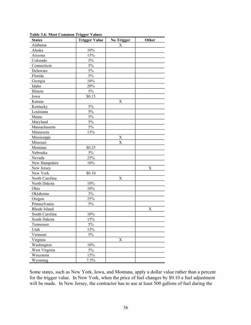
Table 3.6: Most Common Trigger Values States Trigger Value No Trigger Other Alabama X Alaska 10% Arizona 15% Colorado 5% Connecticut 5% Delaware 5% Florida 5% Georgia 10% Idaho 20% Illinois 5% Iowa $0.15 Kansas X Kentucky 5% Louisiana 5% Maine 5% Maryland 5% Massachusetts 5% Minnesota 15% Mississippi X Missouri X Montana $0.25 Nebraska 5% Nevada 25% New Hampshire 10% New Jersey X New York $0.10 North Carolina X North Dakota 10% Ohio 10% Oklahoma 3% Oregon 25% Pennsylvania 5% Rhode Island X South Carolina 10% South Dakota 15% Tennessee 5% Utah 15% Vermont 5% Virginia X Washington 10% West Virginia 5% Wisconsin 15% Wyoming 7.5%
Some states, such as New York, Iowa, and Montana, apply a dollar value rather than a percent for the trigger value. In New York, when the price of fuel changes by $0.10 a fuel adjustment will be made. In New Jersey, the contractor has to use at least 500 gallons of fuel during the
36

month the adjustment is made. Rhode Island will make a fuel adjustment when the cost exceeds $250.
3.5 CONTRACTOR’S CONCERNS
The trigger values imposed in the calculation occur when there is an increase or decrease in the price of fuel. The fuel price adjustment was incorporated so that the price risk fluctuations would be shared when the price of fuel changes. Many contractors across the country, however, do not feel the fuel adjustment covers the changing fuel costs. Although there are complaints about the burden of risk, there is no formal process in place to document or record these types of complaints.
In the state survey, a question to the respective departments of transportation asked if they received any complaints from contractors. Alabama, Florida, Nebraska, Nevada, and New Hampshire responded that when the fuel price drops over the contract periods, they do not receive complaints. Oregon reported that contractors complained when the fuel adjustment did not cover the increased cost of fuel. This same complaint was reported by 23 other states. Kentucky, Montana, Nebraska, New Jersey, South Carolina, and Utah reported that contractors believed more bid items needed to be included. Contractors in New Hampshire felt they had no obligation to pay the state when the price of fuel decreases. In Maine, the contractors working on paving projects wanted a fuel adjustment, while the contractors building structure projects did not. In response to complaints, Iowa asked contractors for alternative solutions. To date, contractors have not responded to this request. California and Texas do not currently have a fuel adjustment, although contractors are requesting one. Michigan does not have a fuel adjustment, but when contractors are asked about instituting an adjustment, the response has been negative.
3.6 STATES OPINION ABOUT PRICE ADJUSTMENT PAYMENT
In the survey, when the question was asked if the fuel adjustment was fair, most responded in the affirmative. The adjustment payment to the contractors is neither too little nor too much to cover the changing price in fuel. Another survey question asked if the state believed the risk was being shared appropriately. The responses from the different departments of transportation are shown in Table 3.7.
37

Table 3.7: States Responses about Fairness and Risk
States Fuel Adjustment Fair? Risk Shared
Appropriately? Alabama Y Y Alaska New Provision Arizona Y Y Colorado Y Y Connecticut Y Y Delaware Y Y Florida Could Not Answer Question Georgia Y Y Idaho Y Y Illinois Y Y Iowa Y Y Kansas Y Y Kentucky N N Louisiana Y Y Maine Y Y Maryland Y Y Massachusetts Y Y Minnesota Y Y Mississippi Y Y Missouri Y Y Montana Y Y Nebraska Y Y Nevada Y Y New Hampshire N N New Jersey Y Y New York Y Y North Carolina Y Y North Dakota Y Y Ohio Y Y Oklahoma Y Y Pennsylvania N Y Rhode Island Y Y South Carolina N Y South Dakota Y Y Tennessee Y Y Utah Y Y Vermont Y Y Virginia Y Y Washington N Y West Virginia Y Y Wisconsin Y Y Wyoming Y Y
Kentucky, New Hampshire, Pennsylvania, and Washington reported that they may pay more to the contractor than the added cost to the fuel price increase. On the other hand, South Carolina suspects the state has not paid the contractor enough to cover the costs, and has added more bid items to remedy this. The state of Utah responded that their method is fair, but contractors do not agree.
38

In terms of risk, Utah also responded that the state believes the risk is being shared appropriately, while the contractors did not. Even though Utah believes the method is fair and the risk is being shared, they are considering changes to the method that will be described later in this report. Kentucky and New Hampshire responded that they are capturing more of the risk than the contractor.
Of the total construction budget, many states are paying a small percentage. Table 3.8 shows which states are paying and the percentage of their budget dedicated to fuel price adjustments.
Table 3.8: Fuel Adjustment Percent of the Annual Total Budget (2008)
States 0%, new provision
Less than 1% More than
4% Don’t know
Don’t use fuel adjustment
Alabama X Alaska X Arizona X Arkansas X California X Colorado X Connecticut X Delaware X Florida X Georgia X Hawaii X Idaho X Illinois X Indiana X Iowa X Kentucky X Louisiana X Maine X Maryland X Massachusetts X Michigan X Minnesota X Mississippi X Missouri X Montana X Nebraska X Nevada X New Hampshire X New Jersey X New Mexico X New York X North Carolina X North Dakota X Ohio X Oklahoma X Oregon X Pennsylvania X Rhode Island X
39

States 0%, new provision
Less than 1% More than
4% Don’t know
Don’t use fuel adjustment
South Carolina X South Dakota X Tennessee X Texas X Utah X Vermont X Virginia X Washington X West Virginia X Wisconsin X Wyoming X Guam X Puerto Rico X
The fuel price adjustment is 5.85 percent and 5 percent for Nebraska and Wyoming, respectively. Kansas did not provide a response to the percent of the total construction budget the state spent on fuel adjustments.
The Table 3.9 shows how much was paid out in fuel price adjustments during 2008.
Table 3.9: Total Amount Paid in Fuel Adjustments for 2008
States $0, new
provision Less than $1 million
Between $1 & $10 million
More than $10 million
Don’t know
Don’t use fuel
adjustment Alabama X Alaska X Arkansas X California X Colorado X Connecticut X Delaware X Florida X Georgia X Hawaii X Idaho X Illinois X Indiana X Iowa X Kentucky X Louisiana X Maine X Maryland X Massachusetts X Michigan X Minnesota X Mississippi X Missouri X Montana X
40

States $0, new
provision Less than $1 million
Between $1 & $10 million
More than $10 million
Don’t know
Don’t use fuel
adjustment Nebraska X Nevada X New Hampshire X New Jersey X New Mexico X New York X North Carolina X North Dakota X Ohio X Oklahoma X Oregon X Pennsylvania X Rhode Island X South Carolina X South Dakota X Tennessee X Texas X Utah X Vermont X Virginia X Washington X West Virginia X Wisconsin X Wyoming X Guam X Puerto Rico X
Delaware and Minnesota stated that it would be difficult to calculate the total amount of fuel adjustments given their current system. Arizona wanted a public information request filed before releasing that information. Kansas was not willing to report how much was spent. As reported by most states, fuel adjustments differed from previous years and varied as construction budgets changed.
Six states gave additional information related to adjustments made in previous years. Missouri reported that in a typical year the fuel adjustment is around $500,000; however, from June to July of 2008, they paid between $3 and $3.5 million. New Hampshire reported that from 2002 to 2008 the range of fuel adjustments was between $46,336 and $2.4 million; the average was $1.2 million. Iowa, Nebraska, Pennsylvania, and South Carolina also provided the fuel adjustments over the last few years (Table 3.10).
41

Table 3.10: Historic Fuel Price Adjustments States 2003 2004 2005 2006 2007 2008 Iowa - $319,832.35 $108,170.94 $712,152.13 $172,764.79 $579,702.79 Nebraska - - - $249,000 $303,000 $319,000 Pennsylvania $819,000 $2,100,000 $9,500,000 $10,400,000 $7,500,000 $17,700,000* S. Carolina -$254,245 $3,568,939 $6,792,962 $6,827,521 $1,782,081 $4,809,340 *As of mid-Oct. 2008
From this small sample, Nebraska and Pennsylvania paid more in 2008 than in earlier years. Iowa and South Carolina paid more in 2006 than 2008.
3.7 NEED FOR CHANGE?
One survey question asked if individual states suspected that changes to the fuel adjustment process may occur in the near future given that there had been dramatic changes in the price of fuel during the summer of 2008. Eight states8 said any changes would depend on the market. Only four states—Montana, New Jersey, Pennsylvania, and West Virginia—stated there would be changes in the near future. In Montana, where the fuel adjustment process is optional to the contractor, the deadline when the contractor can decide to participate will change. New Jersey anticipates that changes will occur, but they are not sure what they will be. Currently in Pennsylvania, for a structure to qualify for a fuel price adjustment the project needs to last at least three months, but this will change to four months. West Virginia will introduce a supplementary specification to make it easier for the contractor to find the fuel index. South Carolina plans to hire Clemson University to develop optimal fuel usage factors.
Five states (Wyoming, California, Michigan, New Mexico, and New Hampshire) gave information on changes that most likely will occur. Wyoming believes they will lower the trigger value which is currently at 7.5 percent. The Associated General Contractors (AGC) met with California a few times requesting to implement a fuel adjustment procedure. The meetings between contractors and the state are frequent when fuel prices are high, but rare when gas prices fall. Michigan has proposed a fuel adjustment process to their contractors several times, but there is no demand. New Mexico plans to incorporate a fuel adjustment process at some point in the future, but not anytime soon. New Hampshire believes that more bid items will be added in the near future.
Utah is currently testing a new method to calculate the fuel adjustment with several of their projects. When the price of fuel increases by more than 15 percent the state will pay a fuel adjustment that will be calculated as shown in Equation 3-3.
( 1.15* )(40 1000)( )
42
COP BOP VWRAdjustment
(3-3)
Where: COP is the current oil price,
BOP is the base oil price, and
8 DE, GA, MN, MO, NE, UT, VA, WA
42

VWR equals the contract price less the cumulative amount invoiced by the Design-Builder, and less Change Orders that have been executed, which will be based upon approved invoice amounts.
When the price of fuel decreases by more than 15 percent the contractor will pay an adjustment that will be calculated as shown in Equation 3-4.
( 0.85* )(40 1000)( )
42
COP BOP VWRAdjustment
(3-4)
The trial method will not have any fuel usage factors for specific bid items.
3.8 SURVEY OVERVIEW
Most states’ fuel adjustment approach is consistent with the general procedure documented in the FHWA Technical Advisory T5080.3. The source for the fuel index and the trigger values, however, show great variation between the states. Some states have modified their process and allowed different bid items for the fuel usage factors to be used, in addition to changing the value of the factors. Only 10 states use a fuel usage factor for structures. It appears that although states did not change their methods based on other states’ procedures (Section 3.2), many states are influenced by how other states apply their fuel adjustments. Few states have performed studies to find an “updated” fuel usage factor value. In 2008, which was not a typical year, significantly more money was paid out by states to contractors, but was still less than 1 percent of the construction budget. In response, many states have made recent changes to their adjustment process for the contractors.
3.9 SURVEY SUMMARY
The survey covered all 50 states and two territories. It was conducted by telephone with the script listed in Appendix A. It started January 12, 2009 and concluded on February 26, 2009. The major findings are:
Implementation across most states was consistent with the FHWA Technical Advisory T 5080.3.
Many states have made changes to the fuel adjustment process.
Source of the fuel price index varies among states.
Trigger value for the fuel adjustment differs between states.
A number of states have received complaints from contractors about the current fuel adjustment method.
Most states believe the current fuel adjustment is fair and the risk is shared appropriately
States have recently or will shortly implement changes to the fuel adjustment.
43

44

4.0 INFLATION INDICES
4.1 BACKGROUND
During the 1970s when the price of fuel increased dramatically, building contractors also increased their bids to absorb the added price risk and costs. FHWA implemented the fuel price adjustment in 1974 so the government would share some of this price risk when fuel prices increase. The method set forth by FHWA for calculating the fuel price adjustment has not changed over 30 years, although some states have changed their process. ODOT stated in September 2007 that “it is very unlikely that those fuel usage factors are accurate or effective in removing the risk of fuel price fluctuations to the grantor or construction firm,” (ODOT “unpublished data”). This chapter evaluates highway construction costs from 1991 to 2008 to determine whether the current fuel price adjustment method appropriately mitigates fuel price risk. Following this analysis, an improved fuel adjustment process is offered for the state of Oregon.
The results found that additional bid items are required when analyzing the total structural construction costs for the state of Oregon. Currently, a number of states track costs for a select number of bid items. FHWA also tracks the costs of these same bid items nationally. Indices assessing structural projects measure three bid items, namely structural concrete, reinforcing steel, and structural steel. No index exists, however, that measures additional costs for structures such as excavation, reinforcement, steel rail, or waterproofing membrane.
Given the unique physical and natural attributes that influence Oregon’s construction costs for different structural bid items, none of the current national indices seemed appropriate. The existing indices track too few bid items. A more appropriate index is one that follows the price of those components that make up a larger proportion of bid prices. Therefore, a new index was developed that captures a larger share of the total construction project for the state of Oregon. The additional bid items and their measurements over time are introduced. Two indices were created that measure costs at the national and Oregon state level. Through a comparison of the two indices, it can be determined whether Oregon’s structural costs are consistent with the rest of the nation. If the costs are not consistent, then the current national fuel usage factors are not appropriate for Oregon.
45

4.2 REVIEW OF CURRENT INDICES
Six states—California, Colorado, Oregon, South Dakota, Utah, and Washington—track the cost trends of the three bid items most frequently used in their construction projects. Each state includes bid items for excavation and surfacing. The major bid items analyzed for structures projects are structural concrete, reinforcing steel, and structural steel. In addition, Colorado, Oregon, and Utah have created a structural index from the composite of the three bid items. The indices from the respective states are represented in Tables 4.1 through 4.6, and bid and construction prices are shown in Figure 4.1 through 4.12.
Table 4.1: California Department of Transportation Average Highway Contract Prices
Year Class "A"
PCC Structure ($/CY)
Reinforcing Steel ($/lb)
Structural Steel ($/lb)
1972 82.08 0.16 0.45 1973 93.60 0.17 0.64 1974 115.19 0.33 0.99 1975 132.10 0.24 0.84 1976 143.05 0.22 0.50 1977 150.03 0.24 1.23 1978 180.77 0.28 0.81 1979 234.24 0.38 1.96 1980 235.45 0.38 1.94 1981 226.84 0.86 2.09 1982 224.72 0.32 2.16 1983 225.84 0.34 2.16 1984 238.48 0.75 2.16 1985 232.39 0.41 2.29 1986 249.74 0.41 2.39 1987 280.40 0.42 2.55 1988 284.55 0.44 3.96 1989 303.49 0.48 3.10 1990 295.24 0.47 2.21 1991 295.21 0.43 2.28 1992 265.31 0.42 3.07 1993 243.79 0.46 2.71 1994 277.92 0.55 2.33 1995 298.80 0.50 2.27 1996 321.88 0.51 2.17 1997 308.54 0.50 2.34 1998 319.95 0.55 2.60 1999 321.22 0.52 3.22 2000 363.59 0.51 2.75 2001 425.17 0.62 3.91 2002 363.50 0.51 3.25 2003 362.75 0.60 1.71 2004 399.64 0.95 5.39 2005 567.31 0.97 2.67 2006 630.16 1.04 3.73 2007 566.25 0.94 6.97 2008 553.62 0.94 5.18
Source: (Luo 2010)
46

0
1
2
3
4
5
6
7
8
1972
1976
1980
1984
1988
1992
1996
2000
2004
2008
$/lb Reinforcing Steel
Structural Steel
Source: (Luo 2010)
Figure 4.1: California’s Historic Reinforcing & Structural Steel Contract Prices
0
100
200
300
400
500
600
700
1972
1975
1978
1981
1984
1987
1990
1993
1996
1999
2002
2005
2008
$/C
Y
Source: (Luo 2010)
Figure 4.2: California’s Historic Structural Concrete Contract Prices
47

Table 4.2: Colorado Highway Construction Cost Index
Year Structural Concrete
Bid Price ($/Cu. Yd.)
Reinforcing Steel Bid Price
($/lb.)
Structural Steel Bid Price
($/lb.)
Structural Index
Base: 1987 1987 $217.32 $0.41 $0.85 100 1988 $195.02 $0.45 $0.89 96.7 1989 $199.41 $0.40 $0.88 95.3 1990 $190.86 $0.37 $0.99 94.1 1991 $195.43 $0.38 $0.89 93.5 1992 $216.87 $0.36 $0.71 94.0 1993 $212.43 $0.37 $0.79 95.3 1994 $219.94 $0.37 $0.67 94.4 1995 $211.29 $0.39 $0.90 98.3 1996 $265.98 $0.43 $1.09 120.2 1997 $246.29 $0.45 $1.01 113.8 1998 $283.01 $0.50 N/A 128.2 1999 $310.56 $0.54 $1.41 145.3 2000 $346.82 $0.47 $1.18 146.8 2001 $303.22 $0.50 $1.29 138.4 2002 $285.35 $0.50 $0.78 121.4 2003 $289.44 $0.55 $0.72 123.4 2004 $323.50 $0.83 $1.26 159.0 2005 $508.77 $0.96 $1.01 210.4 2006 $430.27 $0.92 $2.62 225.1 2007 $546.29 $1.01 $1.40 232.4 2008 $508.40 $1.11 $0.41 241.9
Source: (Bieber 2009)
$0.00
$0.50
$1.00
$1.50
$2.00
$2.50
$3.00
1987
1990
1993
1996
1999
2002
2005
2008
$/lb Reinforcing Steel
Structural Steel
Source: (Bieber 2009)
Figure 4.3: Colorado’s Historic Reinforcing & Structural Steel Bid Prices
48

$0.00
$100.00
$200.00
$300.00
$400.00
$500.00
$600.00
1987
1989
1991
1993
1995
1997
1999
2001
2003
2005
2007
$/C
Y
Source: (Bieber 2009)
Figure 4.4: Colorado’s Historic Structural Concrete Contract Prices
Table 4.3: Oregon Highway Construction Cost Trends
Year Structural Concrete
($/Cu. Yd.) Reinforcing Steel
($/lb.) Structural Steel
($/lb.) Structures Index
Base: 1987 1987 280.91 0.50 0.84 100.0 1988 272.95 0.59 1.54 114.1 1989 329.59 0.51 1.22 118.1 1990 334.66 0.57 0.50 109.9 1991 298.64 0.49 2.08 124.3 1992 267.22 0.51 1.26 104.5 1993 275.37 0.46 1.07 101.0 1994 326.42 0.50 1.21 116.9 1995 379.06 0.59 1.43 136.4 1996 371.92 0.57 1.40 133.4 1997 459.52 0.63 2.39 172.4 1998 411.23 0.67 2.05 157.5 1999 411.87 0.75 3.81 190.2 2000 369.15 0.63 1.49 136.8 2001 319.42 0.65 1.30 123.4 2002 380.43 0.58 1.72 164.1 2003 489.04 0.58 2.28 175.2 2004 410.27 0.80 1.84 159.8 2005 635.51 1.01 1.92 221.8 2006 706.33 1.04 2.41 247.3 2007 772.21 1.11 2.26 263.0 2008 695.13 1.23 2.67 257.6
Source: (ODOT 2007a)
49

0
0.5
1
1.5
2
2.5
3
3.5
4
4.5
1987
1989
1991
1993
1995
1997
1999
2001
2003
2005
2007
$/lb Reinforcing Steel
Structural Steel
Source: (ODOT 2007a)
Figure 4.5: Oregon’s Historic Reinforcing & Structural Steel Bid Prices
0
100
200
300
400
500
600
700
800
900
1987
1989
1991
1993
1995
1997
1999
2001
2003
2005
2007
$/C
Y
Source: (ODOT 2007a)
Figure 4.6: Oregon’s Historic Structural Concrete Bid Prices
50

Table 4.4: South Dakota Department of Transportation Highway Construction Cost Index
Year Class "A" Concrete
($/Cu. Yd.) Reinforcing Steel
($/lb.) Structural Steel
($/lb.) 1987 239.27 0.48 0.62 1988 224.42 0.50 0.90 1989 228.66 0.55 0.69 1990 239.85 0.54 0.92 1991 247.72 0.52 1.06 1992 264.84 0.53 2.00 1993 270.83 0.54 0.61 1994 250.68 0.57 0.67 1995 337.08 0.69 1.22 1996 319.18 0.64 2.08 1997 340.10 0.76 1.27 1998 362.86 0.73 0.93 1999 369.00 0.65 1.19 2000 322.81 0.61 1.02 2001 361.05 0.65 1.07 2002 404.01 0.70 0.91 2003 265.91 0.74 0.93 2004 442.15 2.24 1.09 2005 449.22 1.10 1.40 2006 522.27 1.04 0.46 2007 535.45 1.07 N/A 2008 644.45 1.26 N/A
Source: (SDDOT 2009)
0
0.5
1
1.5
2
2.5
1987
1989
1991
1993
1995
1997
1999
2001
2003
2005
2007
$/lb Reinforcing Steel
Structural Steel
Source: (SDDOT 2009)
Figure 4.7: South Dakota’s Historic Reinforcing & Structural Steel Bid Prices
51

0
100
200
300
400
500
600
700
1987
1989
1991
1993
1995
1997
1999
2001
2003
2005
2007
$/C
Y
Source: (SDDOT 2009)
Figure 4.8: South Dakota’s Historic Structural Concrete Bid Prices
Table 4.5: Price Trends for Utah Highway Construction
Year Structural Concrete
Bid Price ($/Cu. Yd.)
Reinforcing Steel Bid Price
($/lb.)
Structural Steel Bid Price
($/lb.)
Structural Index
Base: 1987 1972 87.11 0.16 0.29 42.2 1973 98.89 0.19 0.36 50.1 1974 123.10 0.36 0.51 69.8 1975 115.99 0.26 0.46 62.2 1976 137.13 0.25 0.44 65.3 1977 153.09 0.28 0.48 72.3 1978 181.72 0.35 0.69 93.8 1979 187.54 0.48 0.72 100.8 1980 189.30 0.39 1.10 122.0 1981 190.48 0.39 0.80 103.7 1982 203.58 0.41 0.68 99.8 1983 181.05 0.36 0.56 85.9 1984 192.96 0.42 0.61 93.4 1985 199.27 0.39 0.69 98.9 1986 195.29 0.35 0.51 85.7 1987 197.59 0.44 0.69 100.0 1988 187.41 0.48 0.81 106.3 1989 184.28 0.47 0.93 112.8 1990 185.71 0.49 1.00 118.0 1991 214.88 0.47 0.78 110.3 1992 232.81 0.47 0.85 118.7 1993 250.34 0.46 0.83 120.9 1994 250.03 0.56 0.88 126.8 1995 192.86 0.74 1.65 167.2
52

Year Structural Concrete
Bid Price ($/Cu. Yd.)
Reinforcing Steel Bid Price
($/lb.)
Structural Steel Bid Price
($/lb.)
Structural Index
Base: 1987 1996 257.99 0.65 1.47 168.0 1997 280.28 0.62 1.18 154.1 1998 279.35 0.64 0.94 140.0 1999 300.84 0.65 1.19 160.4 2000 276.07 0.65 1.07 147.6 2001 308.30 0.65 0.99 149.6 2002 306.97 0.61 1.14 157.3 2003 320.71 0.62 1.23 166.7 2004 313.78 1.01 1.32 182.2 2005 563.88 1.06 2.74 327.4 2006 538.73 1.02 0.54 184.4 2007 554.19 1.11 2.16 290.7 2008 731.62 1.50 2.49 362.6
Source: (UDOT 2009)
0
0.5
1
1.5
2
2.5
3
1972
1976
1980
1984
1988
1992
1996
2000
2004
2008
$/lb Reinforcing Steel
Structural Steel
Source: (UDOT 2009)
Figure 4.9: Utah’s Historic Reinforcing & Structural Steel Bid Prices
53

0
100
200
300
400
500
600
700
800
1972
1975
1978
1981
1984
1987
1990
1993
1996
1999
2002
2005
2008
$/C
Y
Source: (UDOT 2009)
Figure 4.10: Utah’s Historic Structural Concrete Bid Prices
Table 4.6: Washington State Department of Transportation Unit Bid Prices
Year Structural Concrete
Bid Price ($/Cu. Yd.)
Reinforcing Steel Bid Price
($/lb.)
Structural Steel Bid Price
($/lb.) 1990 231.51 0.45 0.82 1991 322.81 0.45 1.04 1992 232.04 0.44 0.97 1993 265.49 0.42 0.88 1994 248.94 0.41 0.71 1995 285.02 0.44 1.34 1996 305.22 0.49 1.17 1997 313.29 0.51 1.37 1998 277.25 0.49 1.03 1999 323.92 0.45 1.12 2000 279.99 0.51 1.15 2001 359.38 0.41 1.17 2002 326.47 0.54 0.94 2003 380.84 0.50 1.13 2004 328.12 0.86 1.31 2005 419.25 0.91 1.50 2006 475.88 0.98 2.67 2007 567.75 1.15 1.70 2008 589.16 1.33 2.95
Source: (WSDOT 2010)
54

0
0.5
1
1.5
2
2.5
3
3.5
1990
1992
1994
1996
1998
2000
2002
2004
2006
2008
$/lb Reinforcing Steel
Structural Steel
Source: (WSDOT 2010)
Figure 4.11: Washington’s Historic Reinforcing & Structural Steel Bid Prices
0
100
200
300
400
500
600
700
1990
1992
1994
1996
1998
2000
2002
2004
2006
2008
$/C
Y
Source: (WSDOT 2010)
Figure 4.12: Washington’s Historic Structural Concrete Bid Prices
FHWA also created a price index for federal-aid highway construction projects since 1972. This index tracks costs for common excavation, surfacing, and structures. The bid items for structures are the same as for the other six states. The composite structures index is calculated from these three items. The respective prices and indices are presented in Table 4.7 and contract prices are shown in Figure 4.13 and 4.14.
55

Table 4.7: Price Trends for Federal-Aid Highway Construction Structures (1987 Base) Reinforcing Steel Structural Steel Structural Concrete
Year Avg. Contract
Price ($/lb.) Index
Avg. Contract Price ($/lb.)
Index Avg. Contract
Price ($/cu. yd.) Index
Structures Index
Base: 1987
1972 .181 41.1 .342 38.6 100.17 41.6 40.7 1973 .207 47.0 .372 42.0 111.81 46.4 45.4 1974 .339 76.9 .551 62.3 136.80 56.8 61.7 1975 .297 67.4 .554 62.6 138.76 57.6 60.6 1976 .258 58.5 .484 54.7 139.59 58.0 57.2 1977 .272 61.7 .520 58.8 143.51 59.6 59.7 1978 .316 71.7 .603 68.1 172.41 71.6 70.7 1979 .421 95.5 .759 85.8 211.33 87.8 88.6 1980 .483 109.6 .941 106.3 226.68 94.1 100.0 1981 .438 99.4 .790 89.3 231.64 96.2 94.9 1982 .407 92.4 .762 86.1 219.63 91.2 90.0 1983 .398 90.3 .708 80.0 213.85 88.8 86.7 1984 .409 92.8 .709 80.1 218.02 90.5 88.2 1985 .444 100.7 .796 89.9 243.60 101.2 98.1 1986 .442 100.3 .850 96.0 236.37 98.2 98.0 1987 .441 100.0 .885 100.0 240.81 100.0 100.0 1988 .494 112.1 .924 104.4 274.12 113.8 111.0 1989 .556 126.2 1.018 115.0 283.40 117.7 118.4 1990 .529 120.0 1.010 114.1 286.18 118.8 117.8 1991 .505 114.6 1.030 116.4 264.98 110.0 112.5 1992 .520 117.9 .916 103.5 259.61 107.8 108.4 1993 .467 106.0 .861 97.3 261.89 108.7 105.3 1994 .515 116.8 .847 95.7 271.94 112.9 109.0 1995 .542 122.9 .922 104.2 302.66 125.7 119.5 1996 .581 121.5 1.068 120.7 293.85 122.0 121.6 1997 .567 128.7 1.186 134.0 320.90 133.2 132.7 1998 .544 123.4 1.111 125.5 337.25 140.0 133.4 1999 .554 125.7 1.224 138.3 342.24 142.1 138.3 2000 .549 124.6 1.351 152.6 363.66 151.0 146.9 2001 .601 136.4 1.201 135.8 339.44 140.9 138.8 2002 .610 138.4 1.436 162.2 374.96 155.7 154.5 2003 .718 162.9 1.219 137.8 406.02 158.5 159.5 2004 .815 184.8 1.521 171.9 331.49 137.6 154.7 2005 .941 213.6 1.571 177.5 394.88 163.9 176.0 2006 .872 197.9 1.736 196.1 574.80 238.7 220.5
Source: (FHWA. 2006b)
56

0
0.2
0.4
0.6
0.8
1
1.2
1.4
1.6
1.8
2
1972
1976
1980
1984
1988
1992
1996
2000
2004
$/lb Reinforcing Steel
Structural Steel
Source: (FHWA 2006b)
Figure 4.13: FHWA’s Historic Reinforcing & Structural Steel Contract Prices
0
100
200
300
400
500
600
700
1972
1974
1976
1978
1980
1982
1984
1986
1988
1990
1992
1994
1996
1998
2000
2002
2004
2006
$/C
Y
Source: (FHWA 2006b)
Figure 4.14: FHWA’s Historic Structural Concrete Contract Prices
The last year recorded for the FHWA index is 2006. After contacting FHWA, we learned the index is no longer calculated.
Figures A-1, A-2, and A-3 in the Appendix B compare the unit prices of structural concrete, reinforcing steel, and structural steel, respectively, for Colorado, Oregon, South Dakota, and Washington. Figures A-4, A-5, and A-6 compare the unit prices of structural concrete, reinforcing steel, and structural steel, respectively, for California, Utah, and the U.S..
57

In Figures A-1 and A-4, unit prices for structural concrete are similar between the seven different sources, although some variability exists. For reinforcing steel, the prices peak in 1981 and 1984 in California, and 2004 in South Dakota. The price of structural steel in Oregon does not demonstrate any relationship with the other states or the U.S. (see Figures A-3 and A-6). Since differences exist in the trends for structural steel, it suggests that Oregon should analyze price trends locally. The three bid items tracked by each of the six states and the U.S. may not be enough to identify the structural construction market. Section 4.3 identifies additional bid items that capture more of the total cost for structural construction.
4.3 FORMATION OF BID ITEM LIST
To identify additional bid items that capture the true cost of structural construction in Oregon, a request was made to ODOT for the 15 most frequently used bid items in the construction for structures. In addition to identifying the most frequently used, the 15 most expensive bid items in terms of individual annual total cost and frequency were also requested. Thorough examination of the most costly bid items in Oregon’s construction contracts determined which bid items existed and weighed heavily on the total construction process, in addition to the frequency. ODOT sent to the research team the list of bid items that met the criteria from 1991 to 2008. Seven of the bid items appeared on both lists. Each bid item with the respective description, frequency, and total dollar amount is shown in Table 4.8.
Table 4.8: Most costly and frequently used structural bid items from 1991 to 2008 Bid Item Item Description Total Cost Frequency Bid Items Most Costly & Frequent 0501-0100000A Bridge Removal Work $65,149,988.53 1133 0510-0100000A Shoring, Cribbing, & Cofferdam $28,623,904.62 854 0530-0100000A Reinforcement $64,311,482.65 1071 0530-0103000A Coated Reinforcement $19,728,636.58 493 0540-0301000A General Structural Concrete, Class 3300 $55,657,472.30 549 0540-0302000A General Structural Concrete, Class 4000 $60,670,164.41 287 0545-0100000J Reinforced Concrete Bridge End Panels $28,809,230.46 660 Remaining Bid Items Most Costly 0510-0101000A Structure Excavation $7,181,939.36 750 0510-0101000K Structure Excavation $5,569,818.55 454 0510-0106000K Granular Wall Backfill $2,495,335.69 330 0510-0108000A Granular Structure Backfill $2,106,531.28 305 0510-0108000K Granular Structure Backfill $2,522,565.34 320 0520-0100000A Furn Pile Driving Equipment $10,581,439.89 617 0520-0303000E Drive PP 12-3/4 X 0.375 Steel Piles $3,712,563.76 240 0520-0330000E Reinforced Pile Tips $1,290,333.54 256 Remaining Bid Items Most Frequent 0510-9Z90000A Section 0510 Misc. $57,993,661.36 42 0540-0303000A General Structural Concrete, Class 5000 $65,176,949.70 124 0540-0307000A General Structural Concrete, HPC4000 $32,960,586.64 117 0540-9Z90000A Section 0540 Misc. $45,770,094.00 195 0550-9Z90000A Section 0550 Misc. $25,736,401.00 27 0550-9Z90000F Section 0550 Misc. $20,157,360.41 43 0560-0100000A Structural Steel $77,386,643.40 176 0596-0104000J Retaining Wall, MSE $50,203,513.83 200
Source: (ODOT “unpublished data”)
58

The first four bid item numbers (e.g. 0501 or 0510) represent the section of work the item falls under.
The dollar values for the different bid items were summed to calculate the total amount spent on the most costly and frequently used structural bid items. The dollar value reported for the respective bid item was then divided by the most costly and frequent structural bid items. All bid items that were reported as being 4 percent9 or higher were placed on a list shown here. Thus, the most frequent and highest in effect items were included.
Bridge Removal Work
Shoring, Cribbing, & Cofferdam
Section 0510 Miscellaneous10
Reinforcement
General Structural Concrete, Class 3300
General Structural Concrete, Class 4000
General Structural Concrete, Class 5000
General Structural Concrete, HPC4000
Reinforced Concrete Bridge End Panels
Structural Steel
Retaining Wall, MSE
After reviewing the list, ODOT made adjustments to accurately reflect the bid items that are used specifically for structures. The authoritative final list of bid items (final list) is documented here.
Structure Excavation
Reinforcement
Coated Reinforcement
General Structural Concrete, Class 3300
General Structural Concrete, Class 4000
General Structural Concrete, Class 4500
General Structural Concrete, Class 5000
Structural Steel
2 Tube Steel Rail
Warranted Waterproofing Membrane
9 Upon visual inspection of the bid items listed, 4 percent appeared to be the best critical point. 10This bid item includes substructure and construction services on design-build projects, shoring and cribbing, controlled low strength structure backfill, etc.
59
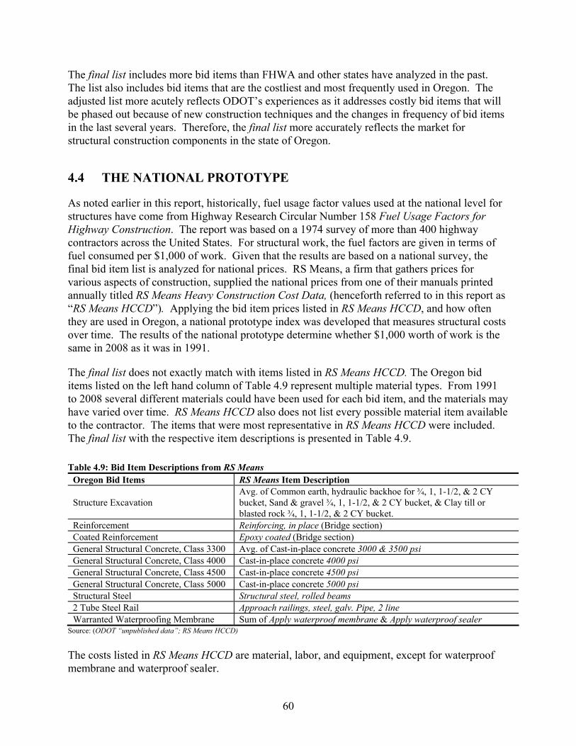
The final list includes more bid items than FHWA and other states have analyzed in the past. The list also includes bid items that are the costliest and most frequently used in Oregon. The adjusted list more acutely reflects ODOT’s experiences as it addresses costly bid items that will be phased out because of new construction techniques and the changes in frequency of bid items in the last several years. Therefore, the final list more accurately reflects the market for structural construction components in the state of Oregon.
4.4 THE NATIONAL PROTOTYPE
As noted earlier in this report, historically, fuel usage factor values used at the national level for structures have come from Highway Research Circular Number 158 Fuel Usage Factors for Highway Construction. The report was based on a 1974 survey of more than 400 highway contractors across the United States. For structural work, the fuel factors are given in terms of fuel consumed per $1,000 of work. Given that the results are based on a national survey, the final bid item list is analyzed for national prices. RS Means, a firm that gathers prices for various aspects of construction, supplied the national prices from one of their manuals printed annually titled RS Means Heavy Construction Cost Data, (henceforth referred to in this report as “RS Means HCCD”). Applying the bid item prices listed in RS Means HCCD, and how often they are used in Oregon, a national prototype index was developed that measures structural costs over time. The results of the national prototype determine whether $1,000 worth of work is the same in 2008 as it was in 1991.
The final list does not exactly match with items listed in RS Means HCCD. The Oregon bid items listed on the left hand column of Table 4.9 represent multiple material types. From 1991 to 2008 several different materials could have been used for each bid item, and the materials may have varied over time. RS Means HCCD also does not list every possible material item available to the contractor. The items that were most representative in RS Means HCCD were included. The final list with the respective item descriptions is presented in Table 4.9.
Table 4.9: Bid Item Descriptions from RS Means Oregon Bid Items RS Means Item Description
Structure Excavation Avg. of Common earth, hydraulic backhoe for ¾, 1, 1-1/2, & 2 CY bucket, Sand & gravel ¾, 1, 1-1/2, & 2 CY bucket, & Clay till or blasted rock ¾, 1, 1-1/2, & 2 CY bucket.
Reinforcement Reinforcing, in place (Bridge section) Coated Reinforcement Epoxy coated (Bridge section) General Structural Concrete, Class 3300 Avg. of Cast-in-place concrete 3000 & 3500 psi General Structural Concrete, Class 4000 Cast-in-place concrete 4000 psi General Structural Concrete, Class 4500 Cast-in-place concrete 4500 psi General Structural Concrete, Class 5000 Cast-in-place concrete 5000 psi Structural Steel Structural steel, rolled beams 2 Tube Steel Rail Approach railings, steel, galv. Pipe, 2 line Warranted Waterproofing Membrane Sum of Apply waterproof membrane & Apply waterproof sealer
Source: (ODOT “unpublished data”; RS Means HCCD)
The costs listed in RS Means HCCD are material, labor, and equipment, except for waterproof membrane and waterproof sealer.
60

The items apply waterproof membrane and apply waterproof sealer only appear in the 1995 to 1999 editions of RS Means HCCD. For the years the bid item does appear in the respective manuals, the value listed is constant across years. ODOT reported that the bid items apply waterproof membrane and apply waterproof sealer did not exist in their database until 2002. Since the bid items do not appear in the manual in the same years as it appears in ODOT’s database, the items were dropped from the list.
The remaining items appear in the 1991 to 2008 editions of the RS Means HCCD. Values for the bid items and available years are shown in Table 4.10, and prices are shown in Figure 4.15 through 4.18.
Table 4.10: National Bid Item Unit Prices
Year
Struct. Excav. ($/CY)
Reinf. ($/lb)
Coated Reinf. ($/lb)
Avg. Class
3000 & 3500
($/CY)
Class 4000
($/CY)
Class 4500
($/CY)
Class 5000
($/CY)
Struct. Steel ($/lb)
Steel Rail
($/LF) 1991 7.77 0.4225 0.9025 51.88 54.3 55.9 57.5 0.6075 62.70 1992 8.18 0.4325 0.9225 52.98 55.1 56.4 57.8 0.6250 63.02 1993 8.06 0.4380 0.8505 48.75 50.5 52.0 53.0 1350 65.25 1994 7.84 0.4410 0.6910 49.75 50.0 52.0 53.0 0.6765 65.44 1995 8.08 0.4445 0.6945 50.25 52.0 53.5 54.0 0.6790 65.65 1996 8.21 0.4580 0.7230 53.00 55.0 56.5 57.0 0.6855 66.86 1997 8.33 0.4850 0.7650 54.75 56.0 57.5 60.0 0.7280 71.12 1998 8.38 0.4950 0.7825 58.25 60.5 62.0 63.5 0.7915 72.88 1999 8.57 0.5000 0.7875 61.00 62.5 63.6 67.5 0.8065 74.69 2000 8.63 0.5075 0.7925 63.75 67.0 69.0 71.5 0.8120 75.50 2001 8.14 0.7000 1.1500 65.50 68.5 70.5 73.0 0.8460 75.96 2002 8.90 0.7200 1.1700 70.00 74.0 75.5 77.0 0.8590 76.45 2003 9.10 0.7275 1.1775 71.75 76.0 77.5 78.0 0.8780 76.79 2004 8.92 0.7350 1.1850 73.25 76.5 78.5 81.0 0.8975 77.21 2005 9.12 0.9025 1.5025 81.50 84.0 86.0 90.0 1.1350 102.50 2006 9.35 0.9725 1.6225 88.00 91.0 93.0 96.0 1.2240 110.48 2007 9.94 1.0450 1.7450 105.00 108.0 110.0 114.0 1.3155 119.11 2008 10.49 1.0925 1.8300 101.50 106.0 109.0 109.0 1.4000 124.65
Source: (RS Means HCCD 2001-2008)
61

0.00
2.00
4.00
6.00
8.00
10.00
12.00
1991
1993
1995
1997
1999
2001
2003
2005
2007
$/C
Y
Source: (RS Means HCCD)
Figure 4.15: National Historic Structural Excavation Bid Item Unit Prices
0
500
1000
1500
2000
2500
3000
3500
4000
1991
1993
1995
1997
1999
2001
2003
2005
2007
$/to
n
Reinforcement
Coated Reinforcement
Structural Steel
Source: (RS Means HCCD)
Figure 4.16: National Historic Reinforcement, Coated Reinforcement, & Structural Steel Bid Item Unit Prices
62

0.00
20.00
40.00
60.00
80.00
100.00
120.00
1991
1993
1995
1997
1999
2001
2003
2005
2007
$/C
Y
Average of Cast-in-place Concrete, Class3000 & 3500
Cast-in-placeConcrete, Class 4000
Cast-in-placeConcrete, Class 4500
Cast-in-placeConcrete, Class 5000
Source: (RS Means HCCD)
Figure 4.17: National Historic Structural Concrete Bid Item Unit Prices
0.00
20.00
40.00
60.00
80.00
100.00
120.00
140.00
1991
1993
1995
1997
1999
2001
2003
2005
2007
$/L
F
Source: (RS Means HCCD)
Figure 4.18: National Historic Steel Rail Bid Item Unit Prices
For all bid items considered, the price in 2008 is higher than the 1991 price. In 2001, the structural excavation price dropped below the price listed in 1996 and also dropped in 2004. Reinforcement, coated reinforcement, and structural steel all experienced steady increases for most years. A significant increase in price for these bid items occurred in 2005. The price of reinforcement and coated reinforcement rose considerably in 2001. Concrete prices rose exponentially from 1991 to 2007 and then decreased in 2008. After 2005, the price of steel rails increased substantially. Therefore, the price for each bid item analyzed has inflated.
63

Compiling the different bid items provided a national prototype. ODOT supplemented the annual total cost of each bid item on the final list for every project from 1972 to 2008 along with the total cost for each of those projects. Class 3300, 4000 and 4500 structural concrete have not been used for a number of years, and were therefore dropped from the national prototype. For future reference, these classes of structural concrete could be added to the national prototype and Oregon State Index. The initial process for developing the national prototype was to calculate the weighted average for each bid item on the final list. The first step for calculating the weighted averages was to determine the annual percentage cost. The annual percentage cost for each bid item on the final list was calculated by taking the annual total cost Oregon spent for each bid item and dividing it by the annual total cost for all six bid items. ODOT was able to acquire this information from 1972 to 2008. Table 4.11 lists the annual percentage costs for each bid item, and the average across all years.
Table 4.11: Annual Percentage Cost of Total Structural Construction for Selected Bid Items
Year Structural Excavation
Reinforcement Coated
Reinforcement
Class 5000
Concrete
Structural Steel
Steel Rail
1972 0.067227 0.372863 0.000000 0.425918 0.112379 0.021614 1973 0.053335 0.348363 0.000000 0.352316 0.223244 0.022742 1974 0.045375 0.566630 0.000000 0.088356 0.297112 0.002526 1975 0.097573 0.628157 0.025467 0.000000 0.201407 0.047396 1976 0.045161 0.268378 0.113939 0.492257 0.076422 0.003843 1977 0.044914 0.305510 0.090777 0.524442 0.004588 0.029768 1978 0.052475 0.329544 0.061292 0.225228 0.328856 0.002606 1979 0.061816 0.477502 0.097757 0.280276 0.059587 0.023062 1980 0.103541 0.370640 0.066258 0.364212 0.087024 0.008325 1981 0.082810 0.226179 0.047514 0.000000 0.621787 0.021710 1982 0.064226 0.289601 0.134757 0.208733 0.292899 0.009784 1983 0.063917 0.321177 0.071642 0.280957 0.247320 0.014987 1984 0.062650 0.300353 0.122859 0.256272 0.220673 0.037194 1985 0.047736 0.226659 0.185324 0.154206 0.331709 0.054365 1986 0.093030 0.358912 0.120794 0.314802 0.081970 0.030492 1987 0.061103 0.511169 0.160981 0.164251 0.092903 0.009593 1988 0.051667 0.067272 0.291902 0.408202 0.178393 0.002564 1989 0.055246 0.174462 0.113882 0.162264 0.481978 0.012167 1990 0.050331 0.260216 0.128456 0.242217 0.312390 0.006390 1991 0.071709 0.296968 0.198772 0.411152 0.015746 0.005655 1992 0.074763 0.286092 0.179964 0.356182 0.079123 0.023877 1993 0.124654 0.274685 0.123150 0.352835 0.106519 0.018157 1994 0.101185 0.221971 0.111654 0.479592 0.049293 0.036306 1995 0.075937 0.293148 0.144866 0.397493 0.027185 0.061371 1996 0.037204 0.187637 0.088581 0.354277 0.327662 0.004639 1997 0.138922 0.248638 0.073855 0.438262 0.072483 0.027840 1998 0.131847 0.342169 0.169078 0.123161 0.215056 0.018689 1999 0.071802 0.328895 0.154768 0.399430 0.030826 0.014279 2000 0.036848 0.181986 0.114200 0.257324 0.358322 0.051320 2001 0.088935 0.328771 0.109169 0.285044 0.169782 0.018299
64

Year Structural Excavation
Reinforcement Coated
Reinforcement
Class 5000
Concrete
Structural Steel
Steel Rail
2002 0.035987 0.262310 0.032949 0.231410 0.419531 0.017813 2003 0.030790 0.168377 0.055486 0.408684 0.328437 0.008227 2004 0.044671 0.420048 0.069951 0.245414 0.208860 0.011056 2005 0.019114 0.217825 0.056472 0.255343 0.449974 0.001271 2006 0.035393 0.489215 0.111185 0.021241 0.337825 0.005141 2007 0.044756 0.315945 0.110328 0.119394 0.407146 0.002432 2008 0.042319 0.274888 0.035771 0.023754 0.615072 0.008195 Average 0.055819 0.286577 0.099340 0.266078 0.277311 0.014876
From 1972 to 1974, coated reinforcement was zero, suggesting that this bid item did not appear in any of the projects during this time. This can be said about Class 5000 concrete in 1975 and 1981. The last row in Table 4.11 is the weighted average for each bid item. Of the six bid items on average reinforcement, structural steel and Class 5000 concrete are the most costly. The average across all years is used as the weighted average since some bid items occur infrequently over time.
All bid items, however, are not measured in the same units. To account for this difference the percentage change in the unit price is calculated each year where 1991 was the base year. The results are presented in Table 4.12.
Table 4.12: National Percentage Change in Price for Selected Bid Items
Year Structural Excavatio
n Reinforcement
Coated Reinforcement
Class 5000 Concrete
Structural Steel
Steel Rail
1991 1.000000 1.000000 1.000000 1.000000 1.000000 1.000000 1992 1.052982 1.023669 1.022161 1.004348 1.028807 1.005104 1993 1.037109 1.036686 0.942382 0.921739 1.111111 1.040670 1994 1.008580 1.043787 0.765651 0.921739 1.113580 1.043700 1995 1.040004 1.052071 0.769529 0.939130 1.117695 1.047049 1996 1.056199 1.084024 0.801108 0.991304 1.128395 1.066348 1997 1.072608 1.147929 0.847645 1.043478 1.198354 1.134290 1998 1.078614 1.171598 0.867036 1.104348 1.302881 1.162360 1999 1.102317 1.183432 0.872576 1.173913 1.327572 1.191228 2000 1.110575 1.201183 0.878116 1.243478 1.336626 1.204147 2001 1.047512 1.656805 1.274238 1.269565 1.392593 1.211483 2002 1.145538 1.704142 1.296399 1.339130 1.413992 1.219298 2003 1.171600 1.721893 1.304709 1.356522 1.445267 1.224721 2004 1.148434 1.739645 1.313019 1.408696 1.477366 1.231419 2005 1.174281 2.136095 1.664820 1.565217 1.868313 1.634769 2006 1.202917 2.301775 1.797784 1.669565 2.014815 1.762041 2007 1.279816 2.473373 1.933518 1.982609 2.165432 1.899681 2008 1.350386 2.585799 2.027701 1.895652 2.304527 1.988038
From 1991 to 2008, according to RS Means HCCD, the largest percentage change was the cost of reinforcement, which increased at the rate of 259 percent. Structural excavation had the smallest percentage change in cost, but still increased by 35 percent. Each of these values in
65

Table 4.12 was multiplied by the respective weighted average where the results are in Table 4.13.
Table 4.13: National Percentage Change in Price Multiplied by Respective Weighted Average
Year Structural Excavatio
n Reinforcement
Coated Reinforcement
Class 5000 Concrete
Structural Steel
Steel Rail
1991 0.055819 0.286577 0.099340 0.266078 0.277311 0.014876 1992 0.058777 0.293360 0.101541 0.267235 0.285299 0.014952 1993 0.057891 0.297090 0.093616 0.245255 0.308123 0.015481 1994 0.056298 0.299125 0.076059 0.245255 0.308808 0.015526 1995 0.058052 0.301499 0.076445 0.249882 0.309949 0.015576 1996 0.058956 0.310656 0.079582 0.263764 0.312916 0.015863 1997 0.059872 0.328970 0.084205 0.277647 0.332316 0.016873 1998 0.060207 0.335753 0.086131 0.293843 0.361303 0.017291 1999 0.061531 0.339144 0.086681 0.312353 0.368150 0.017720 2000 0.061991 0.344231 0.087232 0.330862 0.370661 0.017913 2001 0.058471 0.474802 0.126582 0.337803 0.386181 0.018022 2002 0.063943 0.488367 0.128784 0.356313 0.392115 0.018138 2003 0.065398 0.493454 0.129609 0.360941 0.400788 0.018219 2004 0.064105 0.498542 0.130435 0.374823 0.409689 0.018318 2005 0.065548 0.612155 0.165382 0.416470 0.518103 0.024318 2006 0.067146 0.659635 0.178591 0.444235 0.558730 0.026212 2007 0.071438 0.708811 0.192075 0.527529 0.600498 0.028259 2008 0.075378 0.741030 0.201431 0.504391 0.639070 0.029574
Summing the rows together from Table 4.13 gives the national prototype. The results are in Table 4.14.
Table 4.14: National Prototype Year Index 1991 1.000000 1992 1.021163 1993 1.017455 1994 1.001071 1995 1.011403 1996 1.041737 1997 1.099883 1998 1.154527 1999 1.185579 2000 1.212890 2001 1.401861 2002 1.447660 2003 1.468409 2004 1.495912 2005 1.801976 2006 1.934548 2007 2.128609 2008 2.190873
66

The national prototype represents the total cost for structures from 1991 to 2008. According to the table, the cost of structural projects has more than doubled during this time. Based on this approach with these specific bid items, $1000 work performed in 1991 is not the same as in 2008. Therefore, the fuel usage factor for structures should be reevaluated.
4.5 OREGON STATE INDEX
In addition to the national prototype, an index was created for the state of Oregon. ODOT compiled the unit price for each bid item in the final list from 1972 to 2008. The unit bid item price is the listed unit price from the lowest bid of the three final bid proposals. The unit price includes material, labor, and equipment costs that are consistent with RS Means HCCD. The unit costs for the respective bid items are in Table 4.15 and prices are shown in Figure 4.19 through 4.22.
Table 4.15: Oregon Bid Item Unit Prices
Year
Struct. Excav. ($/CY)
Reinf. ($/lb)
Coated Reinf. ($/lb)
Class 3300
($/CY)
Class 4000
($/CY)
Class 4500
($/CY)
Class 5000
($/CY)
Struct. Steel ($/lb)
2 Tube Steel Rail
($/LF) 1972 5.75 0.16 - - - - 118.13 0.49 14.43 1973 4.57 0.21 - 106.42 116.24 - 132.56 0.34 14.16 1974 7.15 0.44 - 151.16 161.64 - 189.19 0.81 30.91 1975 11.53 0.29 0.63 143.03 144.33 - - 0.76 30.55 1976 9.49 0.23 0.54 158.75 220.75 - 150.18 0.90 23.00 1977 4.38 0.24 0.40 110.06 173.70 145.25 154.33 1.13 32.60 1978 8.07 0.30 0.49 142.56 188.84 195.17 144.27 0.79 35.00 1979 9.07 0.44 0.78 271.00 175.00 249.00 366.00 0.77 37.00 1980 9.62 0.49 0.79 214.04 230.04 204.57 385.16 1.02 62.00 1981 18.49 0.44 0.59 249.96 190.05 210.68 - 1.24 40.87 1982 10.54 0.39 0.56 227.28 266.31 215.22 276.91 0.69 35.21 1983 7.54 0.36 0.51 196.93 235.39 241.79 205.64 0.70 35.69 1984 9.56 0.39 0.56 228.00 251.33 247.95 314.36 1.31 37.41 1985 9.46 0.37 0.55 220.80 215.06 186.85 192.16 0.90 35.60 1986 9.46 0.37 0.50 243.15 227.01 191.06 225.40 1.37 39.23 1987 9.23 0.49 0.52 283.94 259.42 - 306.44 0.98 32.54 1988 14.47 0.45 0.64 233.41 294.83 328.64 402.82 1.21 40.62 1989 14.61 0.45 0.61 325.78 338.95 304.35 287.47 1.18 38.24 1990 20.16 0.43 0.63 312.73 333.52 - 430.59 1.26 45.21 1991 15.87 0.43 0.61 309.56 322.51 - 298.29 2.08 47.07 1992 10.12 0.40 0.65 221.62 298.40 334.81 323.71 1.10 53.28 1993 11.16 0.41 0.60 301.71 229.98 309.03 292.23 1.01 58.03 1994 15.77 0.45 0.62 309.67 367.38 381.41 394.17 1.73 53.76 1995 8.97 0.54 0.75 361.46 496.75 382.32 378.30 1.50 45.44 1996 15.23 0.46 0.71 334.34 433.79 460.59 460.59 1.24 44.81 1997 28.11 0.57 0.61 398.48 - - 657.64 2.47 70.14 1998 17.30 0.56 0.80 287.79 - - 574.31 2.39 58.66 1999 19.98 0.55 0.76 295.09 - - 438.06 1.04 128.82 2000 28.33 0.51 0.71 - - - 484.34 1.41 65.90 2001 18.60 0.61 0.89 - - - 326.29 1.30 65.35
67

Year
Struct. Excav. ($/CY)
Reinf. ($/lb)
Coated Reinf. ($/lb)
Class 3300
($/CY)
Class 4000
($/CY)
Class 4500
($/CY)
Class 5000
($/CY)
Struct. Steel ($/lb)
2 Tube Steel Rail
($/LF) 2002 19.46 0.57 0.67 - - - 447.30 1.72 52.33 2003 19.89 0.54 0.78 - - - 588.56 1.65 77.99 2004 15.00 0.75 1.05 1539.75 - - 478.74 1.76 95.77 2005 20.11 0.93 1.20 466.67 - - 1255.06 1.94 92.82 2006 32.22 0.94 1.07 1472.73 - - 925.10 2.23 171.67 2007 26.68 1.04 1.36 - 1041.67 1005.97 1365.47 2.20 158.43 2008 27.88 1.22 1.36 1159.22 974.61 - 1374.23 3.07 163.22
Source: ODOT, “unpublished data”
0
5
10
15
20
25
30
35
1972
1975
1978
1981
1984
1987
1990
1993
1996
1999
2002
2005
2008
$/C
Y
Figure 4.19: Oregon’s Historic Structural Excavation Bid Item Unit Prices
68

0
0.5
1
1.5
2
2.5
3
3.5
1972
1976
1980
1984
1988
1992
1996
2000
2004
2008
Reinforcement
$/to
n
Coated Reinforcement
Structural Steel
$/L
B
Figure 4.20: Oregon’s Historic Reinforcement, Coated Reinforcement, & Structural Steel Bid Item Unit Prices
0.00
200.00
400.00
600.00
800.00
1000.00
1200.00
1400.00
1600.00
1800.00
1972
1976
1980
1984
1988
1992
1996
2000
2004
2008
$/C
Y
Class 3300 Concrete
Class 4000 Concrete
Class 4500 Concrete
Class 5000 Concrete
Figure 4.21: Oregon’s Historic Structural Concrete Bid Item Unit Prices
69

0
20
40
60
80
100
120
140
160
180
200
1972
1975
1978
1981
1984
1987
1990
1993
1996
1999
2002
2005
2008
$/L
F
Figure 4.22: Oregon’s Historic 2 Tube Steel Rail Bid Item Unit Prices
Overall, the unit prices for the different items have increased in Oregon. The structural excavation price increased significantly in 1981, 1990, 1997, 2000, and 2006, but then dropped the year after. Reinforcement and coated reinforcement showed steady increases for most years except for in 1974 and 1980. A significant price increase for structural steel occurred in 1997 and 1998. The price of concrete rose considerably in 1997, a larger increase existed in 2005 where the price increased by almost four times. Steel rail prices peaked in 1999 and rose again in 2006, which has not decreased since. For each of the structural bid items analyzed, the unit costs have inflated from 1972 to 2008.
Gathering the Oregon unit costs for each bid item yielded an Oregon State Index. Since Class 3500, 4000, and 4500 concrete were not used for a number of years from 1972 to 2008 they were dropped from the list. Dropping these three different concrete types from the list did not have any major impact since they account between 3 and 4 percent of the total structural construction costs. The method for calculating the Oregon State Index is consistent with the process for determining the national prototype. The percentage change in price from 1972 to 2008, using 1991 as the base year, was calculated for Oregon. The results are presented in Table 4.16.
70

Table 4.16: Oregon State Percentage Change in Price for Selected Bid Items
Year Structural Excavation
Reinforcement Coated
Reinforcement Class 5000 Concrete
Structural Steel
2-Tube Steel Rail
1972 0.362319 0.372093 - 0.396011 0.233642 0.306565 1973 0.287965 0.490698 - 0.444392 0.162813 0.300829 1974 0.450536 1.023256 - 0.634245 0.389423 0.656682 1975 0.726528 0.672093 1.037530 - 0.363942 0.649033 1976 0.597984 0.525581 0.891803 0.503470 0.433654 0.488634 1977 0.275992 0.558140 0.655738 0.517382 0.543269 0.692586 1978 0.508507 0.700000 0.809836 0.483657 0.379808 0.743573 1979 0.571519 1.023256 1.278689 1.226994 0.370192 0.786063 1980 0.606175 1.134186 1.291475 1.291227 0.490721 1.317187 1981 1.165091 1.018605 0.960984 - 0.596154 0.868281 1982 0.664146 0.904651 0.916393 0.928325 0.331091 0.748035 1983 0.475110 0.844186 0.840984 0.689396 0.336538 0.758232 1984 0.602394 0.909302 0.921311 1.053874 0.628365 0.794826 1985 0.596093 0.860465 0.901639 0.644205 0.432692 0.756320 1986 0.596093 0.860465 0.819672 0.755640 0.658654 0.833440 1987 0.581601 1.139535 0.852459 1.027322 0.471154 0.691311 1988 0.911783 1.046512 1.049180 1.350431 0.581731 0.862970 1989 0.920605 1.046512 1.000000 0.963727 0.567308 0.812407 1990 1.270321 1.000000 1.032787 1.443528 0.605769 0.960484 1991 1.000000 1.000000 1.000000 1.000000 1.000000 1.000000 1992 0.637681 0.930233 1.065574 1.085219 0.528846 1.131931 1993 0.703214 0.953488 0.983607 0.979684 0.485577 1.232845 1994 0.993699 1.046512 1.016393 1.321432 0.831731 1.142129 1995 0.565217 1.255814 1.229508 1.268229 0.721154 0.965371 1996 0.959672 1.069767 1.163934 1.544101 0.596154 0.952086 1997 1.771267 1.324651 1.004590 2.204710 1.189788 1.490172 1998 1.090107 1.312226 1.314197 1.925324 1.148638 1.246322 1999 1.258979 1.272093 1.244262 1.468558 0.502114 2.736832 2000 1.785129 1.189535 1.157131 1.623724 0.678524 1.400015 2001 1.172023 1.418605 1.455989 1.093853 0.624404 1.388414 2002 1.226213 1.325581 1.098361 1.499547 0.828531 1.111778 2003 1.253201 1.265065 1.282118 1.973122 0.792365 1.656836 2004 0.944928 1.754936 1.716885 1.604933 0.847500 2.034543 2005 1.267410 2.164647 1.971230 4.207516 0.934158 1.971866 2006 2.030372 2.193032 1.757128 3.101348 1.073220 3.647217 2007 1.681386 2.429137 2.234377 4.577659 1.059142 3.365774 2008 1.756587 2.837940 2.231803 4.607037 1.477988 3.467511
Table 4.16 demonstrates that the price of the different construction bid items increased at a greater rate than was reported in RS Means HCCD. The bid item with the greatest percentage price increase was Class 5000 Concrete, which increased by almost 915 percent. The bid item with the smallest percentage change in price was structural excavation which increased 35 percent, the same result as found using the RS Means HCCD.
The weighted averages computed in the last row of Table 4.11 are applied to each row of Table 4.16. Results of this calculation are in Table 4.17.
71
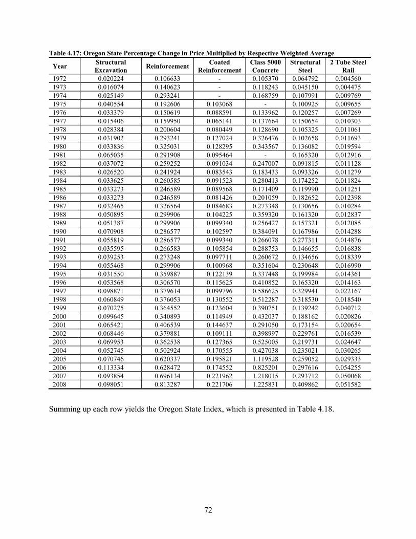
Table 4.17: Oregon State Percentage Change in Price Multiplied by Respective Weighted Average
Year Structural Excavation
Reinforcement Coated
Reinforcement Class 5000 Concrete
Structural Steel
2 Tube Steel Rail
1972 0.020224 0.106633 - 0.105370 0.064792 0.004560 1973 0.016074 0.140623 - 0.118243 0.045150 0.004475 1974 0.025149 0.293241 - 0.168759 0.107991 0.009769 1975 0.040554 0.192606 0.103068 - 0.100925 0.009655 1976 0.033379 0.150619 0.088591 0.133962 0.120257 0.007269 1977 0.015406 0.159950 0.065141 0.137664 0.150654 0.010303 1978 0.028384 0.200604 0.080449 0.128690 0.105325 0.011061 1979 0.031902 0.293241 0.127024 0.326476 0.102658 0.011693 1980 0.033836 0.325031 0.128295 0.343567 0.136082 0.019594 1981 0.065035 0.291908 0.095464 - 0.165320 0.012916 1982 0.037072 0.259252 0.091034 0.247007 0.091815 0.011128 1983 0.026520 0.241924 0.083543 0.183433 0.093326 0.011279 1984 0.033625 0.260585 0.091523 0.280413 0.174252 0.011824 1985 0.033273 0.246589 0.089568 0.171409 0.119990 0.011251 1986 0.033273 0.246589 0.081426 0.201059 0.182652 0.012398 1987 0.032465 0.326564 0.084683 0.273348 0.130656 0.010284 1988 0.050895 0.299906 0.104225 0.359320 0.161320 0.012837 1989 0.051387 0.299906 0.099340 0.256427 0.157321 0.012085 1990 0.070908 0.286577 0.102597 0.384091 0.167986 0.014288 1991 0.055819 0.286577 0.099340 0.266078 0.277311 0.014876 1992 0.035595 0.266583 0.105854 0.288753 0.146655 0.016838 1993 0.039253 0.273248 0.097711 0.260672 0.134656 0.018339 1994 0.055468 0.299906 0.100968 0.351604 0.230648 0.016990 1995 0.031550 0.359887 0.122139 0.337448 0.199984 0.014361 1996 0.053568 0.306570 0.115625 0.410852 0.165320 0.014163 1997 0.098871 0.379614 0.099796 0.586625 0.329941 0.022167 1998 0.060849 0.376053 0.130552 0.512287 0.318530 0.018540 1999 0.070275 0.364552 0.123604 0.390751 0.139242 0.040712 2000 0.099645 0.340893 0.114949 0.432037 0.188162 0.020826 2001 0.065421 0.406539 0.144637 0.291050 0.173154 0.020654 2002 0.068446 0.379881 0.109111 0.398997 0.229761 0.016539 2003 0.069953 0.362538 0.127365 0.525005 0.219731 0.024647 2004 0.052745 0.502924 0.170555 0.427038 0.235021 0.030265 2005 0.070746 0.620337 0.195821 1.119528 0.259052 0.029333 2006 0.113334 0.628472 0.174552 0.825201 0.297616 0.054255 2007 0.093854 0.696134 0.221962 1.218015 0.293712 0.050068 2008 0.098051 0.813287 0.221706 1.225831 0.409862 0.051582
Summing up each row yields the Oregon State Index, which is presented in Table 4.18.
72

Table 4.18: Oregon State Index Year Index 1972 0.301579 1973 0.324564 1974 0.604908 1975 0.446808 1976 0.534078 1977 0.539117 1978 0.554513 1979 0.892995 1980 0.986406 1981 0.630643 1982 0.737308 1983 0.640025 1984 0.852221 1985 0.672081 1986 0.757398 1987 0.857999 1988 0.988503 1989 0.876465 1990 1.026447 1991 1.000000 1992 0.860277 1993 0.823879 1994 1.055583 1995 1.065368 1996 1.066098 1997 1.517014 1998 1.416810 1999 1.129137 2000 1.196512 2001 1.101455 2002 1.202733 2003 1.329239 2004 1.418547 2005 2.294817 2006 2.093429 2007 2.573744 2008 2.820320
The Oregon State Index has tracked a significant percent of the cost for structures from 1972 to 2008. According to the table, the cost of structural projects in Oregon has increased by more than eight and a half times from 1972 to 2008. This further supports for these specific bid items, $1000 of work performed in 1972 is not the same as in 2008 when accounting for inflation of bid item prices.
73

4.6 ANALYSIS
Since the Oregon’s bid items do not correspond exactly to those listed in RS Means HCCD, the percentage change in price is evaluated. The results indicate that the percentage change in price is more varied for the Oregon bid items. Figures 4.23 through 4.28 show price trends for six different items that were applied to the national prototype and the Oregon State Index using 1991 as the base year.
0
0.5
1
1.5
2
2.5
1991
1993
1995
1997
1999
2001
2003
2005
2007
RS Means
Oregon
Oregon Linear Trend
Figure 4.23: Price Percentage Change Trend for Structural Excavation
Figure 4.23 shows the percentage change in price for structural excavation in Oregon is highly varied. A linear trend for Oregon was also calculated that demonstrates the price of structural excavation in Oregon has been increasing over time at a greater rate than RS Means HCCD. From 1991 to 1998 the percentage change in price is lower in Oregon. For the remaining years, it is higher than the RS Means RS Means HCCD except in 2004.
74

0
0.5
1
1.5
2
2.5
3
1991
1993
1995
1997
1999
2001
2003
2005
2007
RS Means
Oregon
Figure 4.24: Price Percentage Change Trend for Reinforcement
Figure 4.24 demonstrates that for steel reinforcement the percentage change in price for Oregon and RS Means HCCD follow the same trend but except from 2001 to 2003 where Oregon is lower.
0
0.5
1
1.5
2
2.5
1991
1993
1995
1997
1999
2001
2003
2005
2007
RS Means
Oregon
Figure 4.25: Price Percentage Change Trend for Coated Reinforcement
The RS Means HCCD percentage change in price is lower every year for coated steel reinforcement, except for 2002 and 2003, as shown in Figure 4.25.
75

0
0.5
1
1.5
2
2.5
3
3.5
4
4.5
5
1991
1993
1995
1997
1999
2001
2003
2005
2007
RS Means
Oregon
Figure 4.26: Price Percentage Change Trend for Class 5000 Concrete
In Figure 4.26, each year the percentage change in price for structural concrete Class 5000 is higher for Oregon, except in 2001 where it dropped below RS Means HCCD.
0
0.5
1
1.5
2
2.5
1991
1993
1995
1997
1999
2001
2003
2005
2007
RS Means
Oregon
Figure 4.27: Price Percentage Change Trend for Structural Steel
After 2000, RS Means HCCD and Oregon’s values for structural steel increase close to the same rate (see Figure 4.27). The percentage change in price is lower every year in the study for Oregon.
76
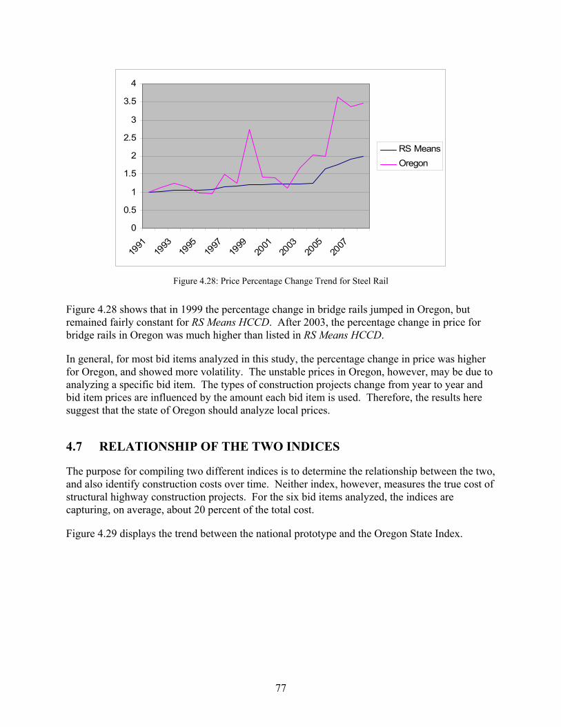
0
0.5
1
1.5
2
2.5
3
3.5
4
1991
1993
1995
1997
1999
2001
2003
2005
2007
RS Means
Oregon
Figure 4.28: Price Percentage Change Trend for Steel Rail
Figure 4.28 shows that in 1999 the percentage change in bridge rails jumped in Oregon, but remained fairly constant for RS Means HCCD. After 2003, the percentage change in price for bridge rails in Oregon was much higher than listed in RS Means HCCD.
In general, for most bid items analyzed in this study, the percentage change in price was higher for Oregon, and showed more volatility. The unstable prices in Oregon, however, may be due to analyzing a specific bid item. The types of construction projects change from year to year and bid item prices are influenced by the amount each bid item is used. Therefore, the results here suggest that the state of Oregon should analyze local prices.
4.7 RELATIONSHIP OF THE TWO INDICES
The purpose for compiling two different indices is to determine the relationship between the two, and also identify construction costs over time. Neither index, however, measures the true cost of structural highway construction projects. For the six bid items analyzed, the indices are capturing, on average, about 20 percent of the total cost.
Figure 4.29 displays the trend between the national prototype and the Oregon State Index.
77

0
0.5
1
1.5
2
2.5
3
1991
1993
1995
1997
1999
2001
2003
2005
2007
RS Means
Oregon
Figure 4.29: Price Percentage Change Trend for the National Prototype and Oregon State Index
Design standards and market forces in Oregon have changed during the time period shown in Figure 4.29, leading to fluctuating prices. The Oregon State Index exhibits more fluctuations between years, and is higher from 2005 to 2008. Oscillations in the Oregon State Index occur because of changes in the demand for the different bid items under investigation. Smaller changes in the RS Means HCCD prices could be due to the fact that the prices listed are averages from several different locations. This suggests that bid item prices in the state of Oregon are harder to predict than listed in RS Means HCCD.
The greatest variability between the two indices is found within the last four years of the study. Oregon bid items prices inflate more than the prices listed in RS Means HCCD. Transforming both indices into a linear trend yielded 0.019 and 0.013 for the Oregon State Index and national prototype, respectively. The standard error for the Oregon State Index and national prototype was 0.0013 and 0.0035, respectively. This implies that the linear trend for Oregon is almost one and one half of the national prototype. The trends also suggest that, on average, construction costs increase between 1 and 2 percent each year. The linear trend for each bid item from the respective source is shown in Table 4.19 where the standard error is in parenthesis.
78

Table 4.19: Linear Trend for Each Bid Item RS Means Oregon
Structural Excavation 0.015893
(0.001903) 0.053973
(0.014679)
Reinforcement 0.095019 (0.00925)
0.091066 (0.012694)
Coated Reinforcement 0.066089
(0.010367) 0.067134 0.010074)
Structural Concrete 0.057303
(0.005662) 0.178744
(0.035489)
Structural Steel 0.068202
(0.007321) 0.024927
(0.011032)
Steel Rail 0.05103
(0.007284) 0.131809
(0.027021)
Of the linear trends from RS Means HCCD the steepest is reinforcement. From Oregon, the two greatest linear trends (structural concrete and steel rail) are around three times more than the linear trend in RS Means HCCD. The remaining bid item trends from Oregon are also approximately three times greater than RS Means HCCD, except for reinforcement and coated reinforcement, which are similar. Bid item weights cause the Oregon State Index and the national prototype trends to be more analogous than the individual bid item trends.
4.8 FORMATION OF TWO ADDITIONAL INDICES
The national prototype measures from 1991 to 2008, while the Oregon State Index begins in 1972. Table 4.7, supplemented by FHWA, reports unit costs on a national level for three bid items ranging from 1972 to 2006. A FHWA index was created based on these three bid items and compared to an adjusted Oregon State Index that is comprised of the same three bid items. The purpose of comparing these two indices is to ascertain the relationship between national and Oregon structural costs over the 37 year time period.
The computation for the FHWA index and the adjusted Oregon State Index is the same as the national prototype and the Oregon State Index. The annual percentage cost for each of the three bid items on the final list was calculated by taking the annual total cost spent in Oregon for each bid item and dividing it by the annual total cost for the three items in the unit costs from Table 4.7 where 1991 is the base year. Table 4.20 lists the annual percentage costs for each bid item, and the average across all years.
79

Table 4.20: Annual Percentage Cost of Oregon’s Total Structural Construction for Selected Bid Items Year Reinforcement Class 5000 Concrete Structural Steel 1972 0.409218 0.467446 0.123336 1973 0.377048 0.381326 0.241627 1974 0.595138 0.092802 0.312061 1975 0.757213 0.000000 0.242787 1976 0.320621 0.588081 0.091299 1977 0.366082 0.628420 0.005497 1978 0.372944 0.254891 0.372165 1979 0.584197 0.342902 0.072902 1980 0.450968 0.443147 0.105884 1981 0.266731 0.000000 0.733269 1982 0.366012 0.263807 0.370180 1983 0.378098 0.330751 0.291152 1984 0.386407 0.329696 0.283897 1985 0.318085 0.216407 0.465508 1986 0.474950 0.416579 0.108471 1987 0.665305 0.213779 0.120916 1988 0.102883 0.624289 0.272827 1989 0.213096 0.198196 0.588708 1990 0.319353 0.297263 0.383384 1991 0.410253 0.567995 0.021752 1992 0.396581 0.493739 0.109680 1993 0.374210 0.480676 0.145114 1994 0.295624 0.638727 0.065649 1995 0.408383 0.553745 0.037872 1996 0.215779 0.407414 0.376807 1997 0.327421 0.577129 0.095449 1998 0.502904 0.181017 0.316079 1999 0.433240 0.526154 0.040606 2000 0.228158 0.322610 0.449232 2001 0.419566 0.363764 0.216670 2002 0.287227 0.253391 0.459382 2003 0.185949 0.451336 0.362715 2004 0.480427 0.280690 0.238883 2005 0.235960 0.276602 0.487437 2006 0.576714 0.025040 0.398247 Average 0.346607 0.351347 0.302047
The last row in Table 4.20 is the weighted average for each of the three bid items analyzed. The percentage change unit price for FHWA’s and Oregon’s three bid items is calculated each year for the unit prices using 1991 as the base year. The results of the percentage change for the three bid items from FHWA and Oregon are presented in Tables 4.21 and 4.22, respectively.
80

Table 4.21: FHWA Percentage Change in Price for Selected Bid Items Year Reinforcing Steel Structural Concrete Structural Steel 1972 0.358416 0.378029 0.332039 1973 0.409901 0.421956 0.361165 1974 0.671287 0.516265 0.534951 1975 0.588119 0.523662 0.537864 1976 0.510891 0.526794 0.469903 1977 0.538614 0.541588 0.504854 1978 0.625743 0.650653 0.585437 1979 0.833663 0.797532 0.736893 1980 0.956436 0.855461 0.913592 1981 0.867327 0.874179 0.766990 1982 0.805941 0.828855 0.739806 1983 0.788119 0.807042 0.687379 1984 0.809901 0.822779 0.688350 1985 0.879208 0.919315 0.772816 1986 0.875248 0.892030 0.825243 1987 0.873267 0.908786 0.859223 1988 0.978218 1.034493 0.897087 1989 1.100990 1.069515 0.988350 1990 1.047525 1.080006 0.980583 1991 1.000000 1.000000 1.000000 1992 1.029703 0.979734 0.889320 1993 0.924752 0.988339 0.835922 1994 1.019802 1.026266 0.822330 1995 1.073267 1.142199 0.895146 1996 1.150495 1.108952 1.036893 1997 1.122772 1.211035 1.151456 1998 1.077228 1.272738 1.078641 1999 1.097030 1.291569 1.188350 2000 1.087129 1.372405 1.311650 2001 1.190099 1.281002 1.166019 2002 1.207921 1.415050 1.394175 2003 1.421782 1.532267 1.183495 2004 1.613861 1.251000 1.476699 2005 1.863366 1.490226 1.525243 2006 1.726733 2.169220 1.685437
81

Table 4.22: Oregon Percentage Change in Price for Selected Bid Items Year Reinforcement Class 5000 Concrete Structural Steel 1972 0.372093 0.396011 0.233642 1973 0.490698 0.444392 0.162813 1974 1.023256 0.634245 0.389423 1975 0.672093 - 0.363942 1976 0.525581 0.503470 0.433654 1977 0.558140 0.517382 0.543269 1978 0.700000 0.483657 0.379808 1979 1.023256 1.226994 0.370192 1980 1.134186 1.291227 0.490721 1981 1.018605 - 0.596154 1982 0.904651 0.928325 0.331091 1983 0.844186 0.689396 0.336538 1984 0.909302 1.053874 0.628365 1985 0.860465 0.644205 0.432692 1986 0.860465 0.755640 0.658654 1987 1.139535 1.027322 0.471154 1988 1.046512 1.350431 0.581731 1989 1.046512 0.963727 0.567308 1990 1.000000 1.443528 0.605769 1991 1.000000 1.000000 1.000000 1992 0.930233 1.085219 0.528846 1993 0.953488 0.979684 0.485577 1994 1.046512 1.321432 0.831731 1995 1.255814 1.268229 0.721154 1996 1.069767 1.544101 0.596154 1997 1.324651 2.204710 1.189788 1998 1.312226 1.925324 1.148638 1999 1.272093 1.468558 0.502114 2000 1.189535 1.623724 0.678524 2001 1.418605 1.093853 0.624404 2002 1.325581 1.499547 0.828531 2003 1.265065 1.973122 0.792365 2004 1.754936 1.604933 0.847500 2005 2.164647 4.207516 0.934158 2006 2.193032 3.101348 1.073220
The average weights found in the last row of Table 4.20 are multiplied by each row in Table 4.21 and 4.22. The weight reinforcement is multiplied by the FHWA bid item Reinforcing Steel. Class 5000 Concrete weight is multiplied by the FHWA bid item Structural Concrete. Structural Steel appears in both tables. The results of this computation are in Tables 4.23 and 4.24, respectively.
82

Table 4.23: FHWA Percentage Change in Price Multiplied by Respective Weighted Average Year Reinforcing Steel Structural Concrete Structural Steel 1972 0.124229 0.132819 0.100291 1973 0.142074 0.148253 0.109089 1974 0.232673 0.181388 0.161580 1975 0.203846 0.183987 0.162460 1976 0.177078 0.185088 0.141933 1977 0.186687 0.190285 0.152490 1978 0.216887 0.228605 0.176829 1979 0.288953 0.280210 0.222576 1980 0.331507 0.300563 0.275947 1981 0.300621 0.307140 0.231667 1982 0.279344 0.291215 0.223456 1983 0.273167 0.283552 0.207620 1984 0.280717 0.289081 0.207914 1985 0.304739 0.322998 0.233426 1986 0.303367 0.313412 0.249262 1987 0.302680 0.319299 0.259526 1988 0.339057 0.363466 0.270962 1989 0.381610 0.375770 0.298528 1990 0.363079 0.379457 0.296182 1991 0.346607 0.351347 0.302047 1992 0.356902 0.344226 0.268616 1993 0.320525 0.347250 0.252488 1994 0.353470 0.360575 0.248382 1995 0.372002 0.401308 0.270376 1996 0.398769 0.389627 0.313190 1997 0.389160 0.425493 0.347794 1998 0.373374 0.447172 0.325800 1999 0.380238 0.453789 0.358937 2000 0.376806 0.482190 0.396180 2001 0.412496 0.450076 0.352192 2002 0.418673 0.497173 0.421106 2003 0.492799 0.538357 0.357471 2004 0.559375 0.439535 0.446032 2005 0.645855 0.523586 0.460694 2006 0.598497 0.762148 0.509081
83

Table 4.24: Oregon Percentage Change in Price Multiplied by Respective Weighted Average Year Reinforcement Class 5000 Concrete Structural Steel 1972 0.128970 0.139137 0.070571 1973 0.170079 0.156136 0.049177 1974 0.354667 0.222840 0.117624 1975 0.232952 - 0.109928 1976 0.182170 0.176892 0.130984 1977 0.193455 0.181781 0.164093 1978 0.242625 0.169931 0.114720 1979 0.354667 0.431100 0.111815 1980 0.393116 0.453668 0.148221 1981 0.353055 - 0.180066 1982 0.313558 0.326164 0.100005 1983 0.292600 0.242217 0.101650 1984 0.315170 0.370275 0.189796 1985 0.298243 0.226339 0.130693 1986 0.298243 0.265492 0.198944 1987 0.394970 0.360946 0.142310 1988 0.362728 0.474469 0.175710 1989 0.362728 0.338602 0.171353 1990 0.346607 0.507179 0.182971 1991 0.346607 0.351347 0.302047 1992 0.322425 0.381288 0.159736 1993 0.330485 0.344209 0.146667 1994 0.362728 0.464281 0.251222 1995 0.435273 0.445588 0.217822 1996 0.370788 0.542515 0.180066 1997 0.459133 0.774618 0.359372 1998 0.454826 0.676456 0.346942 1999 0.440916 0.515973 0.151662 2000 0.412301 0.570490 0.204946 2001 0.491698 0.384322 0.188599 2002 0.459455 0.526861 0.250255 2003 0.438480 0.693250 0.239331 2004 0.608273 0.563888 0.255985 2005 0.750281 1.478297 0.282159 2006 0.760119 1.089649 0.324163
Summing each row in Table 4.23 yields the FHWA Index, which is presented in Table 4.25.
84

Table 4.25: FHWA Index Year Index 1972 0.357340 1973 0.399416 1974 0.575641 1975 0.550293 1976 0.504098 1977 0.529462 1978 0.622321 1979 0.791740 1980 0.908018 1981 0.839428 1982 0.794016 1983 0.764339 1984 0.777711 1985 0.861164 1986 0.866040 1987 0.881505 1988 0.973485 1989 1.055909 1990 1.038717 1991 1.000000 1992 0.969745 1993 0.920262 1994 0.962427 1995 1.043685 1996 1.101586 1997 1.162447 1998 1.146346 1999 1.192963 2000 1.255176 2001 1.214764 2002 1.336952 2003 1.388627 2004 1.444942 2005 1.630135 2006 1.869726
Summing each row in Table 4.24 yields the adjusted Oregon State Index, which is presented in Table 4.26.
85

Table 4.26: Adjusted Oregon State Index Year Index 1972 0.338678 1973 0.375392 1974 0.695131 1975 0.342879 1976 0.490046 1977 0.539328 1978 0.527276 1979 0.897583 1980 0.995005 1981 0.533121 1982 0.739727 1983 0.636468 1984 0.875241 1985 0.655276 1986 0.762679 1987 0.898227 1988 1.012907 1989 0.872683 1990 1.036756 1991 1.000000 1992 0.863449 1993 0.821361 1994 1.078230 1995 1.098684 1996 1.093370 1997 1.593122 1998 1.478225 1999 1.108551 2000 1.187737 2001 1.064618 2002 1.236571 2003 1.371061 2004 1.428145 2005 2.510737 2006 2.173931
The relationship between the FHWA Index and the Adjusted Oregon State Index are shown in Figure 4.30.
86

0
0.5
1
1.5
2
2.5
3
1972
1975
1978
1981
1984
1987
1990
1993
1996
1999
2002
2005
FHWA
Adjusted OregonState Index
Figure 4.30: Price Percentage Change Trend for the FHWA Index and Adjusted Oregon State Index
Figure 4.30 demonstrates the relationship between the FHWA Index and the adjusted Oregon State Index from 1972 to 2006. For the three bid items being analyzed, the relation between the two indices is similar. From 1981 to 1994, the adjusted Oregon State Index is a little lower in magnitude, except in 1984. In the late 1990s, the opposite holds true where the adjusted Oregon State Index is larger. Similarly, during last recorded years, the adjusted Oregon State Index was much higher. The purpose of these two indices is to extend structural costs back to 1972. The indices provide further support that $1000 worth of work is not the same from 1972 to 2006.
4.9 SUMMARY OF INDICES
The national prototype, Oregon State Index, and the FHWA Index demonstrate that the price for structural construction has increased. The indices also show the magnitude of the price increase. The national prototype and the Oregon State Index examine this change for six different bid items, from 1991 to 2008. The FHWA Index and the adjusted Oregon State Index, however, measure this change from 1972 to 2006, but for only three bid items. The indices demonstrate that the price of structural construction changes each year, which implies that $1,000 worth of work is not the same between years. Therefore, alternatives to the current method are necessary.
Highway Research Circular Number 158: Fuel Usage Factors for Highway Construction, from which the values for the fuel usage factors originated, suggests that fuel usage factors for structures are given in terms of fuel consumed per $1,000 of work. The publication may not have anticipated the effects of inflation when proposing the specific fuel usage factors. Based on the survey of states, 10 have structural bid items listed where the respective fuel usage factor is multiplied by the monthly fuel used instead of fuel consumed per $1,000 of work. If implemented in Oregon, this alternative method would exclude the changes in structural construction costs that occur.
87

88
The national prototype constructed in this study demonstrates how structural construction costs have changed from 1991 to 2008. Volatility of prices between years and sources indicate that the state of Oregon should apply local prices when analyzing construction costs. Hence, an Oregon State Index was created to demonstrate how structural construction costs have behaved from 1991 to 2008. Volatility in construction prices suggest that this index may need to be calculated annually. An automated process could be developed to measure annual changes. The current results exemplified that structural costs have inflated by more than double. Assuming fuel efficiency of construction vehicles has not changed, a $1,000 of work in 1991 is less than $500 of work in 2008. Since the fuel usage factor for structures is fuel consumed per $1000 of work, the fuel price adjustment from structures is twice as much in 2008 than in 1991. This result suggests that the fuel usage factor for structures should be revaluated from the current standard of 19 and 10 diesel gallons per $1000 of work.

5.0 CONCLUSIONS AND RECOMMENDATIONS
Most state departments of transportation allow specific fuel price adjustments in highway contracting. The fuel price adjustments are calculated using the monthly consumption of fuel for selected commodities multiplied by a fuel factor when the price of fuel changes by a certain amount. Fuel Usage Factors for Highway Construction, published in 1974, details the values for the fuel usage factors. Because of economic forces in the highway construction market, price adjustments occur that do not happen in other government contracts. In other markets, price adjustments are almost nonexistent.
The variability in the approach for calculating fuel adjustments in the western U.S. and Florida led to a national survey. All fifty states, Puerto Rico, and Guam responded to a series of questions about whether fuel adjustments were instituted in their state, how it was calculated, how long it had been around, and if there were problems with the current method. Since 1980, when Development and Use of Price Adjustment Contract Provisions was published and outlined how the fuel price adjustment should be calculated, most states have made changes to the method, and some have changed the fuel usage factor values. In some states the adjustment was dissolved in the late 1980s or early 1990s and then reintroduced when fuel prices increased in 2008. Most states that have a fuel price adjustment receive complaints from contractors when the price of fuel decreases, or as happened in 2008, when the price of fuel increases dramatically. Still, most states believe the risk is shared appropriately. For the states that track how much is paid in fuel price adjustments, the average annual fuel price adjustment in 2008 was around $8 million, which is less than 1 percent of the total annual budget.
After conducting the national survey, construction costs overtime were examined. The number of bid items analyzed was narrowed down to the six most costly and frequently used. All bid items, individually and collectively, showed an upward trend nationally and for Oregon at the state level. The fuel usage factor for structures is given in terms of fuel consumed per $1000 of work. Results of the national prototype and the Oregon State Index suggest that $1000 worth of work is not consistent from 1991 to 2008.
The upward trend for both indices revealed that the current fuel usage factor for structures is not appropriately current. Examining the prices for individual bid items shows that when the fuel usage factor is measured by fuel consumed per $1000 of work, the fuel usage factor should fluctuate reflecting construction cost variability.
The above findings lead to the following two specific recommendations for implementation; 1) the fuel factors for structures, the focus of this study, should be changed from 19 for cast-in-place and 10 for pre-cast to 9 for cast-in-place and 5 for pre-cast, to reflect the impact of inflation on construction costs; and 2) after 35 years of not incorporating the impact of construction cost increases on the fuel factors, and with this study as a new base, the fuel factors (gallons per $1,000 of construction value) should be reviewed and recalculated every three years, so as to keep the factors current and equitable.
89

90
The increasing structural construction costs may lead to a decrease in the number of bids. An incentive for changing this pattern, however, would be to hold fuel usage factors at 1980 levels where the average annual fuel price adjustment is less than 1 percent of the total annual budget.
Future research could determine if budget losses from fuel price adjustments would be offset by contractors making lower bids. Additionally, information gathered from the survey for this study found variation across states in values triggering adjustments. While an assessment of trigger values was not a focus of the project, it was noted that Oregon was at the higher end of the continuum. Further investigation of trigger values could be a potential avenue for future research and policy consideration by ODOT.
Structural construction costs are not the only aspect of the construction process that is changing. The type and amount of bid items used varies from year to year. One bid item heavily used in the construction process may be replaced by another in subsequent years. It would also be interesting to study the short and long term program budget impacts as a result of utilizing different fuel factors/trigger values and how price risk is shifted between the state and contractors during economic expansion or recession. This research has not addressed this issue, but future research may be able to track program cost (payments) over time and make comparisons between periods of volatile price changes and program cost under different fuel factor/trigger regimes.
Regardless, it is important that every few years ODOT reevaluate the adjustment process and whether the current six bid items carry the same weight in the construction process. The conclusions of this report suggest that prices change continually and that the variables examined need to be monitored routinely.

6.0 REFERENCES
AASHTO Subcommittee on Construction, Contract Administration Section. Survey on the Use of Price Adjustment Clauses. www.fhwa.dot.gov/programadmin/contracts/2008aashto.cfm. Accessed November 2008.
Alan M. Voorhees Transportation Center et al. Fuel Price Adjustment Techniques: A Review of Industry Practice. September 2004. www.policy.rutgers.edu/vtc/documents/InstAnal.Fuel Pricing.pdf. Accessed June 2008.
Bieber G. Colorado Construction Cost Index Report. Colorado Department of Transportation. July 2009. http://www.coloradodot.info/business/eema/documents/2009/2009Q2CCI.pdf/view. Accessed June 2008.
Carroll et al. A Study of Fuel Price Adjustments. Georgia State Department of Transportation, Report GDOT RP 06-06. June 2006.
Colorado Department of Transportation. Fuel Cost Adjustment Notice. November 30, 2006. www.dot.state.co.us/DesignSupport/Construction/2005SpecsBook/2005SSP/109fca.doc. Accessed February 2009.
FHWA. Construction Contract Administration. Summary of Responses: AASHTO/FHWA Survey on Construction Cost Increases and Competition. April 2006a. www.fhwa.dot.gov/program admin/contracts/priccomp.cfm. Accessed April 2008. FHWA. Price Trends for Federal-Aid Highway Construction. 2006b. www.fhwa.dot.gov/programadmin/pt2006q1.pdf. Accessed February 2007. FHWA. Development and Use of Price Adjustment Contract Provisions. Technical Advisory T 5080.3, Dec. 10, 1980. www.fhwa.dot.gov/programadmin/ contracts/ta50803.cfm. Accessed January 2008. Florida Department of Transportation. Standard Specifications for Road & Bridge Construction. 2007. ftp://ftp.dot.state.fl.us/LTS/CO/Specifications/SpecBook/2007Book/009.pdf Accessed June 2008. Idaho Transportation Department. Fuel Price Adjustment. January 2008. Integrated Acquisition Environment. Federal Acquisition Regulation. www.acquisition.gov/far/index.html
91

92
Luo, Z. Price Index for Selected Highway Construction Items. January 2010. http://www. dot.ca.gov/hq/esc/oe/contract_progress/cost-index-summary.pdf. Accessed May 2009.
Oregon Department of Transportation. Oregon Highway Construction Cost Trends. www.oregon.gov/ODOT/HWY/ESTIMATING/docs/cost_trends/Table08_01.pdf. Accessed February 2007a. Oregon Department of Transportation. Asphalt & Fuel Prices 2003-2007. www.oregon.gov/ODOT/HWY/ESTIMATING/asphalt_fuel.shtml. Accessed February 2007b. Oregon Department of Transportation. ODOT Monthly Fuel Price History. www.oregon.gov/ODOT/HWY/ESTIMATING/docs/asphalt_fuel_pricesfuel_price_history.pdf. Accessed February 2007c. Oregon Department of Transportation. Steel Escalation/De-Escalation. www.oregon.gov/ODOT/HWY/ESTIMATING/steel.shtml. Accessed February 2007d Platts. Oilgram Price Report. www.platt.com. Accessed April 2010. RS Means. Heavy Construction Cost Data. Kingston, MA. (Example 2009 Annual Report https://www.rsmeans.com/bookstore/detail.asp?sku=60169 Accessed May 2010) South Dakota Department of Transportation. South Dakota Highway Construction Cost Index. July 2009. www.sddot.com/pe/projdev/docs/CCI-LET20091STHALF.DOC. Accessed February 2009. Utah Department of Transportation. Construction Cost Index Report. October 2009. www.udot.utah.gov/main/uconowner.gf?n=8428710288600675. Accessed February 2009. Utah Department of Transportation. 2008 Individual Standard Specifications, January 2008. www.udot.utah.gov/main/f?p=100:pg:0:::1:T,V:1925. Accessed June 2008. Washington State Department of Transportation (WSDOT). Special Provisions January 2008. http://www.wsdot.wa.gov/publications/fulltext/projectdev/gspspdf/egsp1.pdf. Accessed June 2008. Washington State Department of Transportation. WSDOT Unit Bid Prices. April 2010. http://www.wsdot.wa.gov/biz/Construction/CostIndex/pdf/BidPrices.pdf. Accessed June 2008. Wyoming Department of Transportation (WYDOT). Supplemental Specification for Fuel Adjustment. April 2008. www.dot.state.wy.us/webdav/site/wydot/shared/Construction/ Supplemental%20Specifications/Division%20100/SS100J_Fuel%20Adjustment%20Rev%2010-01-09.pdf. Accessed June 2008.

APPENDIX A: TELEPHONE STATE SURVEY


TELEPHONE SCRIPT FOR NATIONAL SURVEY
1. Name of respondent
2. Position of respondent
3. Phone number of respondent
4. We are investigating at the national level the current use of fuel factors so as to determine the structure and magnitude of the factors, and identify any issues felt by the DOTs regarding these factors. We appreciate your help with this survey.
5. If you are not the appropriate person within the DOT to answer these questions, could you please direct me to the person knowledgeable of these issues?
6. Please describe the current process e.g. minimum qualifications, factor levels,
application timing, etc. your state uses in dealing with the issue of increasing fuel costs during the construction period? Let’s discuss this.
7. Does your state utilize a process that is described in detail in a
publication/manual? Where can I get the specific detail, Web site? Publication? Etc.
8. Is the price adjustment and fuel factors related to any index or is it a fixed factor,
e.g. 19 gallons /$1,000 of construction for structures?
9. In your knowledge, how was the process decided upon for your state and how long has it been at this stage/level? By this we mean the percentage before a project qualifies, the level of the fuel factor, especially for structures, how and when payments are made, etc. etc.
10. Have there been any significant changes in the process or level of fuel factors
over the years?
11. Are any changes being discussed at the current time? By whom and for what known reason?
12. What alternatives to your current system are being considered?
13. Do you expect any changes in the near future?
14. If so, can you estimate what they might look like and what would be the dominant
reason that the changes would be instituted?
A-1

A-2
15. Are you familiar with any studies that have been done on fuel factors in your state, region or anywhere? Could you help us find them?
16. Do you receive complaints or concerns with the current methods used for the
price adjustment?
17. Do they come from contractors? Are the concerns with the minimum qualifications, the fuel factor magnitude, the number of bid items that are in the fuel factor? Do the contractors offer alternatives?
18. Does the State or you as the official feel the current methods pay out either too much or too little to the contractor?
19. Does the State or you feel the risk isn’t being shared appropriately?
20. What aspect of the process would the State be interested in changing?
21. If there were problems and concerns before the price of fuel went up so dramatically, what were the source and the type of concerns? Was it DOT, legislators, contractors, etc.?
22. Did this lead to any proposed changes?
23. Could give us a rough estimate of how many of your projects might qualify for a
price adjustment, such as fuel factors?
24. What rough percentage of the total construction budget would have price adjustments such as fuel factors?
25. In fact, would you be able to give us a magnitude of $ paid out in fuel factors in a
typical or recent year? eg. 1.5 million dollars in a yearly budget?
Table A.1: Summary of Telephone Survey Description Number of States
Number of Respondents 50 + Puerto Rico
&Guam Number of Specifications Engineers 7 Number of Assistant Construction Engineers
4
States Use Fuel Adjustment 42 Fuel Adjustment in Standard Specifications Manual
10
Fuel Adjustment is a Special Provision 24 Did not answer Questions 24 & 25 6
Source: Results from telephone survey

APPENDIX B: HISTORIC UNIT PRICES


$0.00
$100.00
$200.00
$300.00
$400.00
$500.00
$600.00
$700.00
$800.00
$900.00
1987
1989
1991
1993
1995
1997
1999
2001
2003
2005
2007
Cu
. Y
d.
CO
OR
SD
WA
US
Figure B.1 Historic Unit Price of Structural Concrete
1987-2008 Colorado, Oregon, South Dakota, Washington, & the US
$0.00
$0.50
$1.00
$1.50
$2.00
$2.50
1987
1989
1991
1993
1995
1997
1999
2001
2003
2005
2007
lb.
CO
OR
SD
WA
US
Figure B.2 Historic Unit Price of Reinforcing Steel
1987-2008 Colorado, Oregon, South Dakota, Washington, & the US
B-1

$0.00
$0.50
$1.00
$1.50
$2.00
$2.50
$3.00
$3.50
$4.00
$4.50
1987
1989
1991
1993
1995
1997
1999
2001
2003
2005
2007
lb.
CO
OR
SD
WA
US
Figure B.3 Historic Unit Price of Structural Steel
1987-2008 Colorado, Oregon, South Dakota, Washington, & the US
0
100
200
300
400
500
600
700
800
1972
1975
1978
1981
1984
1987
1990
1993
1996
1999
2002
2005
2008
Cu
. Y
d. CA
UT
US
Figure B.4 Historic Unit Price of Structural Concrete
1972-2008 California, Utah, & the US
B-2

B-3
0
0.2
0.4
0.6
0.8
1
1.2
1.4
1.6
1972
1975
1978
1981
1984
1987
1990
1993
1996
1999
2002
2005
2008
lb.
CA
UT
US
Figure B.5 Historic Unit Price of Reinforcing Steel
1972-2008 California, Utah, & the US
0
1
2
3
4
5
6
7
8
1972
1975
1978
1981
1984
1987
1990
1993
1996
1999
2002
2005
2008
lb.
CA
UT
US
Figure B.6 Historic Unit Price of Structural Steel
1972-2008 California, Utah, and the US