evaluation of impact and fatigue properties of austempered ductile iron … · ·...
TRANSCRIPT

Evaluation of Impact and Fatigue properties of Austempered Ductile Iron
MARCO DAL COROBBO AND SERGIO ARIAS
© Marco Dal Corobbo and Sergio Arias, 2009.
No.
Masters Thesis:
Department of Materials and Manufacturing Technology
Chalmers University of Technology
SE-412 96 Göteborg
Sweden
Telephone: + 46 (0)31-772 12 50
Printed by Chalmers Reproservice
Göteborg, Sweden 2009

Evaluation of Impact and Fatigue properties of Austempered Ductile Iron
MARCO DAL COROBBO AND SERGIO ARIAS
Department of Materials and Manufacturing Technology
Abstract
Austempered Ductile Iron (ADI) proved to be an excellent material as it possesses
attractive properties: high strength, ductility and toughness are combined with good wear
resistance and machinability. In this work impact and the fatigue properties have been
evaluated for low alloyed Austempered Ductile Iron. To do this, Charpy-type impact test for
austempered ductile iron was performed by the standard ASTM A 327M and Fatigue
Crack Growth Rates (FCGR) were measured by the standard ASTM E 647. It was found
that impact energy is related with the morphology of the graphite nodules in the
microstructure. In particular, the impact energy increases when the nodularity and the
nodule count increase, and the nodule size decreases. A clear relation with the amount of
retained austenite wasn’t found. For the fatigue properties it was found that these were
related with the morphology of microstructure (graphite nodules, amount of retained
austenite and its carbon content). However, it was observed that the the crack initiation
was mainly affected by the presence of defects as porosity or carbides. When the
preferential crack path was observed between two neighboring nodules, the crack growth
rate increased when two graphite nodules were closer. The growth of the crack depends
on the orientation of the ferrite laths, but, in this work, it was observed that the crack path
probably takes place along the austenite/ferrite interface. Furthermore, it was found that
the likelihood of crack formation, facilitated by decohesion of the graphite nodules,
increased with nodule size.

Preface This diploma thesis is based on work carried out in the Department of Materials and
Manufacturing Technology at Chalmers University of Technology, during the autumn of
2008 and spring of 2009.

Acknowledgements We want to take advantage of the following lines to express our gratitude with all the
people which contribute to the success in finishing the present work.
Our first mention and special thanks are destined to our supervisors in Sweden, Henrik
Borgström and Kenneth Hamberg from the department of Materials and Manufacturing
Technology at Chalmers, for their guidance and experience on the topic. Their constructive
criticism and discussions during the work served us to achieve a high level of
understanding. We wish also to thank Prof. Lars Nyborg, from the department of Materials
and Manufacturing Technology of Chalmers, for giving us the opportunity to carry out this
work, and our supervisors in Italy and Spain, Professor Alberto Molinari from the University
of Trento, José Manuel Torralba and Monica Campos of Carlos III University in Madrid, for
giving us the opportunity to study abroad, and for supporting us with this work.
We also want to mention the staff of the department of Materials and Manufacturing
Technology who despite of not being involved directly in this work, still unselfishly helped
us with our tasks. To all of them thanks, but we are especially grateful for the support
provided by Dr. Peter Sotkovszki and Dr. Yiming Yao.
Final mentions, the last but not the least, is for our families, for giving us the opportunity to
study abroad and the support during all the time spent far from home. Special thanks also
to all our “home” friends and all the “new” friends met in our unforgettable experience in
Sweden.
Sergio Arias and Marco Dal Corobbo

INDEX
1. INTRODUCTION .............................................................................................................1
2. AN OVERVIEW OF AUSTEMPERED DUCTILE IRON ...................................................2
2.1. History of Austempered Ductile Iron ...........................................................................3
2.2. Market and applications of Austempered Ductile Iron.................................................3
3. THE MICROSTRUCTURE AND HEAT TREATMENT OF AUSTEMPERED DUCTILE
IRON ................................................................................................................................6
3.1. The microstructure of Austempered Ductile Iron.........................................................6
3.2. Heat treatment cycle of Austempered Ductile Iron......................................................9
3.3. Influence of heat treatment on properties of Austempered Ductile Iron ....................16
4. INFLUENCE OF MICROSTRUCTURE ON THE IMPACT PROPERTIES OF
AUSTEMPERED DUCTILE IRON..................................................................................25
4.1. Effect of austenitization conditions on impact properties of Austempered Ductile Iron
.......................................................................................................................................25
4.2. Effect of austempering conditions on impact properties of Austempered Ductile Iron
.......................................................................................................................................29
4.3. Effect of alloy elements segregation on impact properties of Austempered Ductile
Iron.................................................................................................................................32
5. INFLUENCE OF MICROSTRUCTURE ON THE FATIGUE PROPERTIES OF
AUSTEMPERED DUCTILE IRON..................................................................................34
5.1. High Cycle Fatigue of Austempered Ductile Iron ......................................................38
5.2. Low Cycle Fatigue of Austempered Ductile Iron .......................................................43
5.3. Low Cycle Fatigue of Austempered Ductile Irons at various strain ratios .................46
5.4. Mechanism of fatigue crack growth in Austempered Ductile Iron .............................49
5.5. Influence of heat treatment on fatigue crack growth of Austempered Ductile Iron ....51
5.6. Effect of carbides on fatigue characteristics of Austempered Ductile Iron ................55
5.7. Effect of Titanium content on fatigue properties of Austempered Ductile Iron ..........56
6. MATERIAL, EXPERIMENTS AND CHARACTERIZATION ...........................................57
6.1. Material .....................................................................................................................57
6.2. Heat treatment ..........................................................................................................58
6.3. Characterization........................................................................................................59
6.4. Fracture mechanism analysis ...................................................................................64
6.5. Impact test ................................................................................................................65
6.6. Fatigue Crack Growth Rate test................................................................................66
7. RESULTS AND DISCUSSION ......................................................................................71
7.1. Characterization........................................................................................................71
7.1.1. Light Optical Microscope......................................................................................71
7.1.2. X-Ray analysis .....................................................................................................77
7.1.3. Porosity................................................................................................................79
7.1.4. Hardness .............................................................................................................80
7.1.4. Carbide study.......................................................................................................82
7.2. Impact test ................................................................................................................87
7.3. Fracture mechanism analysis ...................................................................................98
7.4. Fatigue Crack Growth Rate test..............................................................................103
8. CONCLUSION.............................................................................................................115
9. REFERENCES ............................................................................................................117

1
1. INTRODUCTION Our highly developed technological society continues to exert enormous demand for light,
durable and cost effective materials. This is why we continually look for new materials that
combine excellent mechanical properties and characteristics as well as improving those
already in service. In recent years there has been significant interest in the properties and
development of Austempered Ductile Iron. This Austempered Ductile Iron, ADI, refers to
ductile iron that undergoes a heat treatment called austempering. It appears that ADI
could be developed into a major engineering material with a wide range of versatile
engineering properties.
Therefore, the context of this work has been to evaluate the impact and fatigue properties
of different alloys and heat treatments proposed in collaboration with the foundry
Componenta, in order to improve the alloy as well as developing a more feasible industrial
heat treatment. The impact and fatigue properties were chosen because they are
important features for the material application. Moreover an extensive literature survey
was conducted to compare our materials with others, but also to try to propose a new point
of discussion or find suggestions for future studies.
The present work is a continuation of Caroline Glondu [5] and Javier Hidalgo [4] master
thesis’ conducted at Chalmers University of Technology, with a different direction.

2
2. AN OVERVIEW OF AUSTEMPERED DUCTILE IRON Austempered Ductile Iron (ADI), also known as ausferritic ductile iron, is the most recent
addition to the ductile iron family. It is produced by giving conventional ductile iron a
special heat treatment called “austempering” [2]. The austempering heat treatment
transforms ductile iron to ADI, bringing about excellent strength, toughness, and fatigue
characteristics. ADI is stronger per unit weight than aluminium, as wear resistant as steel
and has the potential for up to 50% cost savings [3].
For the designer ADI is a most versatile material, enabling innovative solutions to new and
current problems. By selecting precise heat treatment parameters a specific set of
properties can be achieved. The lower hardness ductile iron castings are used in structural
applications, often where weight and cost reduction are important. Wear resistance is
superior to steel at any given hardness level, making the higher hardness grades ideal for
mining, construction, agricultural and similar high abrasion applications [3].
ADI competes favourably with steel forgings, especially for heavy-duty parts where
reliability is paramount. It is used to upgrade from standard ductile irons, and as a
substitute for manganese steel and nickel-hard materials. When strength is required ADI is
particularly cost-effective: tensile and yield values are twice as high as standard ductile
iron; fatigue strength is 50% higher and it can be enhanced by shot peening or fillet rolling.
With its high strength-to-weight ratio ADI can even replace aluminium when reduced
section sizes are acceptable [3].

3
2.1. History of Austempered Ductile Iron The austempering process is neither new nor novel and has been utilized since the 1930's
on cast and wrought steels [2]. In fact this kind of heat treatment had been applied on steel
in 1933 and on grey cast iron in 1937 [5].
Nearly 50 years after its discovery ADI is still widely regarded as a "new material". A major
reason for this was the slow commercialisation of the austempering process. ADI
remained a laboratory curiosity until 1972, the year when the austempering process was
firstly commercially applied to the ductile iron, when a limited facility was set up to process
a small compressor crankshaft in the USA [3]. However the first truly viable commercial
service was delayed until the introduction of new furnace developments at Applied
Process Inc in Michigan during 1984 [3]. Since the 70’s, considerable process modelling
and material evaluation has followed, resulting in wider understanding and acceptance of
ADI [3].
In the latter nineties the development of Ductile Iron introduced the use of thin walled
parts, in order to increase the strength to weight ratio and its competitiveness against
lighter alloys [18].
2.2. Market and applications of Austempered Ductile Iron Over the most recent twenty years, heat treatment specialists and equipment engineers
have refined the austempering process and plants to enable reliable production of high
grade austempered materials. This has fuelled demand and a family of austempered Irons
and Steels are now routinely produced. Of these ADI is becoming the material of choice as
designers and engineers, which seek cost effective performance from their components
and systems. In particular, manufacturers engaged in moving parts and safety critical
items have benefited from increased strength, greater wear resistance, noise reduction
and weight saving [7]. ADI is now established in many major markets [7] as seen in Figure
2.1.

4
Figure 2.1: ADI treatment market distribution 2004, adapted from [7].
In Farm Machinery and Equipment the equipment used in farming is subjected to high
wear and heavy loads. Performance is constantly being pushed to the next level as
products are expected to last longer and be cost effective. The agricultural industry has
therefore taken a keen interest in ADI and other austempered materials for their excellent
wear characteristics.
In Heavy Truck, economic growth drives the need to haul heavier loads over longer
distances, resulting in more time between vehicle maintenance and some difficult
engineering challenges. The Heavy Truck industry recognised the potential benefits of
austempering solutions many years ago. Manufacturers took advantage of the versatility of
ADI to introduce innovative light weight, high performance parts.
In Machinery Conveyors and Tooling markets have benefited greatly by incorporating ADI
and other austempered alloys in their equipment designs. Lighter weight, easier to
manufacture castings have made components less expensive, last longer and reduced the
weight of individual tools or material handling systems.
In the Railway Industry products, improvements in safety and transport efficiency: wear
plates, suspension housings and suspension covers are examples of ADI application.

5
Construction Equipment can benefit greatly from the use of tough, wear resistant
austempered Irons and Steels. Whether for ground engaging components such as bucket
teeth or engine and powertrain parts, ADI and other austempered materials can improve
the performance of the heavy duty equipment.
For high performance gear and powertrain manufacturers, austempered materials offer
greater wear resistance, reduced noise, improved bending and contact fatigue, as well as
increased strength and durability.
Austempering an iron, steel, or powdered metal component (depending on the specific
application) can therefore deliver a valuable competitive edge. Companies such as Delphi
Automotive, Dana Corporation, Ford Motor Company, AGCO, John Deere, and General
Motors are among those selecting ADI and austempered steels for production and design.
The automotive industry is constantly looking to increase performance, reduce the cost
and weight of the vehicles they produce, to boost the drive for lower emission as well as
better fuel economy.
Austempered materials have a proven track record of providing strength and dependability
for safety components, suspension systems, and drivetrain applications.
In Mining/Forestry Equipment the difficult applications and large scale engineering
demand high performance and set intriguing design problems. ADI has met these
challenges, providing improved strength and wear resistance, as seen in heavy-duty
components.
Even the sports goods industry has adopted ADI for its high strength to weight and
superior wear resistance: bobsleigh runners, sword blades, gun components are examples
of ADI application for this kind of industry.

6
3. THE MICROSTRUCTURE AND HEAT TREATMENT OF AUSTEMPERED DUCTILE IRON 3.1. The microstructure of Austempered Ductile Iron The factor that characterizes ADI is the property of combining good elongation and
toughness with high tensile strength, which is a combination that increases the resistance
to wear and fatigue when compared to other ductile irons. These desirable mechanical
properties are associated with a unique austempered microstructure which consist of
graphite nodules, acicular, carbide free ferrite with carbon-enriched austenite, rather than
ferrite and carbide, as produced in normal bainitic transformation in steel [8]. When steel is
austempered, the resulting microstructure consist of fine dispersion of carbide in a ferrite
matrix called bainite. In ductile cast iron, the presence of a large amount of silicon
suppressed the carbide formation. This microstructure in ADI be called “ausferrite” to
distinguish it from the bainite structure in steels [9].
During the austempering transformation, ADI goes through a two-stage reaction. In the
first stage, austenite transforms to a structure of acicular ferrite and carbon-enriched
retained austenite. When ferrite forms within the austenite during the austempered
process of nodular or ductile cast iron, the carbon is rejected from these regions and goes
into solution in the surrounding austenite. As more and more ferrite forms, the carbon
content of austenite increases. Since the carbon content of this austenite is very high (in
excess of 1.0%), the austenite is stable in room temperature and hence the resulting
microstructure consist of ferrite and high carbon and stable austenite [10]. This is the
desired structure that provides the remarkable properties in ADI. In the second stage,
when the casting is austempered longer than required for the above structure, the carbon-
enriched austenite further decomposes into ferrite and carbide. In the latter case the iron
contains large amount of carbide and the matrix become brittle. Therefore this reaction is
undesirable and must be avoided.
The microstructure and mechanical properties of ADI can be greatly altered by suitable
heat treatment process, thus the microstructure of ADI strongly depends on austempering
temperature and time. Austempering to high temperatures gives place to the production of
relatively thick ferrite laths in an austenite matrix enriched in carbon. When austempering

7
is carried out at lower temperatures, thinner needles of acicular ferrite result (Figure 3.1). If
austempering time is very short, the degree of advance of the transformation is less than
100% and a percentage of untransformed austenite remains, that could transform to
martensite during cooling. If austempering time is too long, as the second stage of
transformation begins, Carbon precipitates in the form of carbides as described above
[10].
Figure 3.1: examples of matrix microstructures: as-cast DI and ADI austenized at 950°C
and austempered at 360°C for 1 and 3 hours, respectively. Courtesy of Glondu [5].
The best mechanical properties in ADI are obtained after the completion of the first
reaction but before the onset of the second reaction [27]. This time interval between the
completion of the first reaction and the onset of the second reaction is known as the
process window and it defines a restricted time-temperature domain in which the
austempering heat treatment is to be carried out [26, 27]. The minimum time required for a
given austempering temperature is defined by the presence in the final microstructure of
ADI of no more than 3% martensite, while the maximum allowed austempering time
correlates with the 90% of high carbon austenite still remained in the microstructure [26]. A
successful model for the prediction of the processing window has been developed using a
model for the isothermal transformation of austenite in high Si (>1,5 %wt) steels [34, 35],
literature data and a linear regression technique [36, 37]. The modelling of the process
window for various ADI compositions provides a guide to choosing a minimum
austempering time (close to the lower boundary) to achieve the ASTM standard and
simultaneously reduce the heat treatment costs [26]. In Figure 3.2 is shown an ADI
8
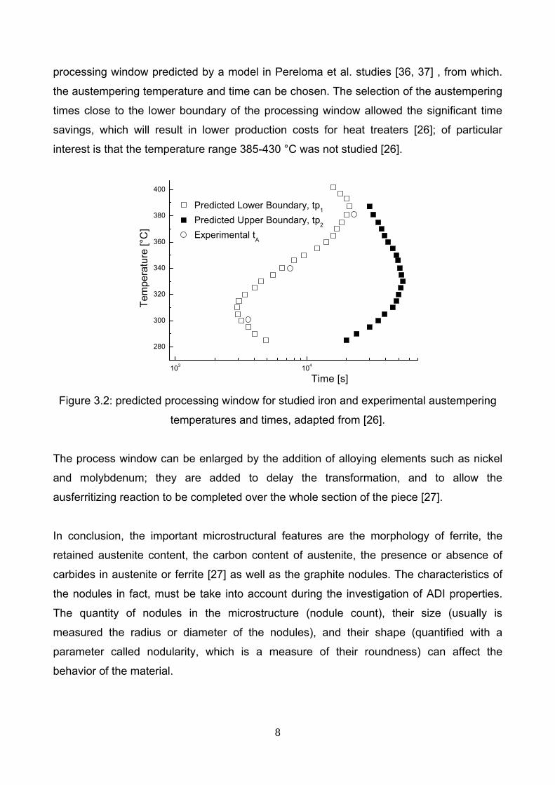
processing window predicted by a model in Pereloma et al. studies [36, 37] , from which.
the austempering temperature and time can be chosen. The selection of the austempering
times close to the lower boundary of the processing window allowed the significant time
savings, which will result in lower production costs for heat treaters [26]; of particular
interest is that the temperature range 385-430 °C was not studied [26].
103 104
280
300
320
340
360
380
400
Predicted Lower Boundary, tp1
Predicted Upper Boundary, tp2
Experimental tA
Tem
pera
ture
[°C
]
Time [s] Figure 3.2: predicted processing window for studied iron and experimental austempering
temperatures and times, adapted from [26].
The process window can be enlarged by the addition of alloying elements such as nickel
and molybdenum; they are added to delay the transformation, and to allow the
ausferritizing reaction to be completed over the whole section of the piece [27].
In conclusion, the important microstructural features are the morphology of ferrite, the
retained austenite content, the carbon content of austenite, the presence or absence of
carbides in austenite or ferrite [27] as well as the graphite nodules. The characteristics of
the nodules in fact, must be take into account during the investigation of ADI properties.
The quantity of nodules in the microstructure (nodule count), their size (usually is
measured the radius or diameter of the nodules), and their shape (quantified with a
parameter called nodularity, which is a measure of their roundness) can affect the
behavior of the material.

9
3.2. Heat treatment cycle of Austempered Ductile Iron
ADI is produced by an isothermal heat treatment known as austempering, which is carried
out to obtain the “ausferrite” microstructure in ductile iron. The complete ADI heat
treatment cycle consists of four main stages: austenitization, quenching to the
austempering temperature, austempering, cooling to room temperature (Figure 3.3).
All the different stages are of significance in determining the exact microstructure
produced and each specific property is determined by the careful selection of heat
treatment parameters.
Tem
pera
ture
Time
A1
Ms
Austenitization
Air cool
Isothermal Transformation
HeatQuench
Figure 3.3: illustration of typical ADI heat treatment cycle, adapted from [11].
The Austenitization process During austenitization, the cast component is usually heated between 850 and 950 °C for
about 15 minutes to 2 hours [4]. The austenitization temperature and time are important
factors that affect the microstructure and the mechanical properties of ADI. The optimum
temperature and time depend on the chemical composition of the ductile iron, the graphite
nodule count and the process variables like casting section size and type [6]. They have to
be controlled to ensure formation of fine grain austenite and uniform carbon content in the
matrix [11].
The austenitizing temperature controls the carbon content of the austenite which, in turn,
affects the structure and properties of the austempered casting [6]. The austenitizing

10
temperature should be selected to ensure sufficient carbon transfer from the graphite
nodule to the matrix occurs [5]. Furthermore, all carbides and particles need to be
dissolved as well as allowing the segregated elements to even out in the matrix [5].
At high austenitizing temperatures, the diffusion of the carbon is faster, the concentration
of impurity elements at the austenite grain boundaries is lower leading to a reduction of
segregations, but the austenite grain is larger leading to a coarse acicular ferrite structure
[1]. Thus, when the austenitizing temperature increases, the amount of retained austenite
and the carbon content of the austenite increase, which is favourable for the toughness
properties and for increasing its hardenability, but making transformation during
austempering more problematic and potentially reducing mechanical properties after
austempering (the higher carbon austenite requires a longer time to transform to
ausferrite) [5, 6]. On the other hand, a too low austenitizing temperature should cause an
incomplete austenitization and may affect the mechanical properties, by the presence of
cell boundary cementite/carbide [5, 11]. Therefore, it is necessary to select a high enough
temperature to obtain a homogeneous austenitic matrix, to minimize the enrichment of
impurity elements at the grain boundaries and to increase the carbon content of the
austenite in order to improve the toughness properties, but also not too high temperature
to reduce the mechanical properties after austempering [5, 6].
The austenitization time should be long enough to ensure the heat of the entire part to the
desired austenitization temperature to obtain the stability of the retained austenite through
the saturation of the austenite with the equilibrium level of carbon, (typically about 1.1-
1.3%) [5, 6]. Furthermore, the austenitization time should be as short as possible in order
to avoid grain growth, but long enough to eliminate the risk of cementite phase in the
austenite [5]. In addition to the casting section size and type, the austenitization time is
affected by the chemical composition, the austenitization temperature and the nodule
count [5, 11].
The Quenching process The quenching is the stage of heat treatment cycle of ADI where the casting is quenched
from the austenitization temperature to the austempering temperature, where the
isothermal transformation is carried out.

11
The cooling rate must be controlled to avoid formation of pearlite around the carbon
nodules, which would reduce mechanical properties [11]. Usually quench time must be
controlled within a few seconds to avoid the pearlite nose in the isothermal transformation
diagram (Figure 3.4). Furthermore, the casting must not be quenched to temperatures
below the point of martensite formation (Ms) [4, 5, 11].
Austempering is fully effective only when the cooling rate of the quenching apparatus is
sufficient for the section size and hardenability of the component [4,11].
There are several critical aspects which must be controlled: transfer time from the
austenitizing environment to the austempering environment, quench severity of the
austempering bath, maximum section size and type of casting being quenched,
hardenability of the castings [11].
Figure 3.4: isothermal transformation diagram for an ADI alloy, courtesy of J. Hidalgo.
Therefore, from the point of view of optimum mechanical properties, it is desirable that in
the austempering heat treatment of ductile iron the structure over the whole cross-section
of the casting should consist of acicular ferrite and retained austenite, in which no pearlite
and proeutectoid ferrite occur [1]. For this purpose it is possible to evaluate the critical bar
diameter (Dc) for a particular composition of ADI or adjust the chemical composition to
avoid segregation during quenching for a particular bar diameter. The critical bar diameter
is a measure of the “austemperability” of ADI, and it is referred to the ability to cool a

12
ductile iron rapidly enough to form ausferrite and thereby avoid eutectoid (stable and
metastable) transformation. The value of critical austempering diameter Dc give cooling
conditions that guarantee a matrix structure with 99% ausferrite matrix in the centre of
cylinder [1]. There are several regressions functions that can be used to calculate the
critical bar diameter, one proposed by Voigt and Lopper [24] is:
Where %Cγ is the carbon content of austenite after quenching, TA the austenitizing
temperature, and T is the austempering temperature. The austenite carbon content that
depends on the austenitizing temperature and silicon content, can be calculated with the
following equation proposed by Voigt [25]:
The quenching process may take place in various media. The most common media used
is molten salt (nitrate) bath, because it allows rapid and efficient heat transfer with a
uniform low viscosity over the austempering temperature range. Moreover, it remains
stable during the process and dissolves easily in water which is positive for subsequent
removing and cleaning operations [28]. The disadvantage of this media is that it pollutes
the environment, in a way that is comparable to a fertilizer.
Water is another media could be used: it is inexpensive, readily available and seldom
contaminated but it isn’t advised as the resulting rapid cooling rates increases the risk of
vapour entrapment [29]. Another issue is that water is present only as steam over a
temperature of 100 °C.
The other possibilities are oil and gas quenching. Oil is seldom used because its chemical
instability limits its applications below 245 °C [28] but, despite of this disadvantage, oil is
preferred as a quenching medium to minimize stresses [30].
Gas quenching is used to provide a cooling rate faster than that obtained in still air and
slower than that for oil, where the cooling rate can be adjusted and controlled by factors

13
like pressure and gas type [29]. However, as high pressures are required to adequately
quench the parts, gas quenching is only feasible for smaller parts.
The Austempering process The austempering step, where the ausferrite transformation occurs isothermally, is the
stage that determines the final microstructure of the casting. Austempering time and
temperature must be controlled to obtain the desired microstructure in order to have
optimum mechanical properties.
As described above, during austempering, a two-stage phase transformation reaction
takes place. In the first stage, austenite (γ) decomposes into ferrite (α) and high carbon
content or untransformed austenite (γHC). In the second stage the high carbon austenite
(γHC) decomposes into ferrite (α) and ε-carbide:
1st reaction:
2nd reaction:
The presence of ε-carbide due to the too long holding time at austempering temperature
must be avoided because resulting in the embrittlement of the matrix.
In order to obtain the best mechanical properties in ADI the process must be carried out
after the completion of the first reaction but before the onset of the second reaction. This
time interval between the completion of the first reaction and the onset of the second
reaction is known as the process window. The process window could be modified by
addition of alloying elements, so the process also depend on the chemical composition of
the casting [1, 4, 5].
Austempering temperature is one of the major determinants of the mechanical properties
of ADI castings [6]. To produce ADI with lower strength and hardness but higher
elongation and fracture toughness, a higher austempering temperature (350-400 °C)
should be selected to produce a coarse ausferrite matrix with higher amounts of carbon
stabilized austenite (20-40%) [6]. Instead, to produce ADI with higher strength and greater
wear resistance, but lower fracture toughness, austempering temperatures below 350 °C
should be used (Figures 3.5 and 3.6) [6].

14
250 275 300 325 350 375 4000
200
400
600
800
1000
1200
1400
1600
1800
0.2%
Offs
et Y
ield
Stre
ngth
[MP
a]
Austempering Temperature [°C] Figure 3.5: ADI yield strength vs. austempering temperature, adapted from [6].
240 260 280 300 320 340 360 380 4000
2
4
6
8
10
12
14
Elo
ngat
ion
(%)
Austempering Temperature [°C] Figure 3.6: ADI elongation vs. austempering temperature, adapted from [6].
Once the austempering temperature has been selected, the austempering time must be
chosen to optimize properties through the formation of a stable structure of ausferrite [6].
At short austempering times, there is insufficient diffusion of carbon to the austenite to
stabilize it, and martensite may form during cooling to room temperature. The resultant
microstructure would have a higher hardness but lower ductility and fracture toughness
(especially at low temperatures) [6]. The minimum time required for a given austempering
temperature is defined by the presence in the final microstructure of ADI of no more than
3% martensite [26]. Excessive austempering times can result in the decomposition of

15
ausferrite into ferrite and carbide (bainite) which will exhibit lower strength, ductility and
fracture toughness (Figure 3.7) [6].
Figure 3.7: schematic diagram showing the effect of austempering time on the amount and
stability of austenite and the hardness of ADI, adapted from [6].
100 101 102 103 104
Ms T
empe
ratu
re o
f Sta
biliz
ed A
uste
nite
+ 20 °C
100 101 102 103 104
Stab
ilized
Aus
teni
te C
onte
nt
MARTENSITE
AUSTENITE
BAINITE
100 101 102 103 104
Har
dnes
s H
B
Trasformation Time (Ti) [min]
16
The Cooling process
By the end of austempering step, the desired ADI ausferrite structure has developed and
thus the casting is ready to cool down. The final cooling is an important stage as other
steps such as austempering conditions or chemical composition. Usually the specimen
was air cooled to room temperature because it is the most economical way [1]. The reason
because caution has to be paid in this step is to maintain the correct microstructure
obtained in the previous stages to room temperature without contaminate it.
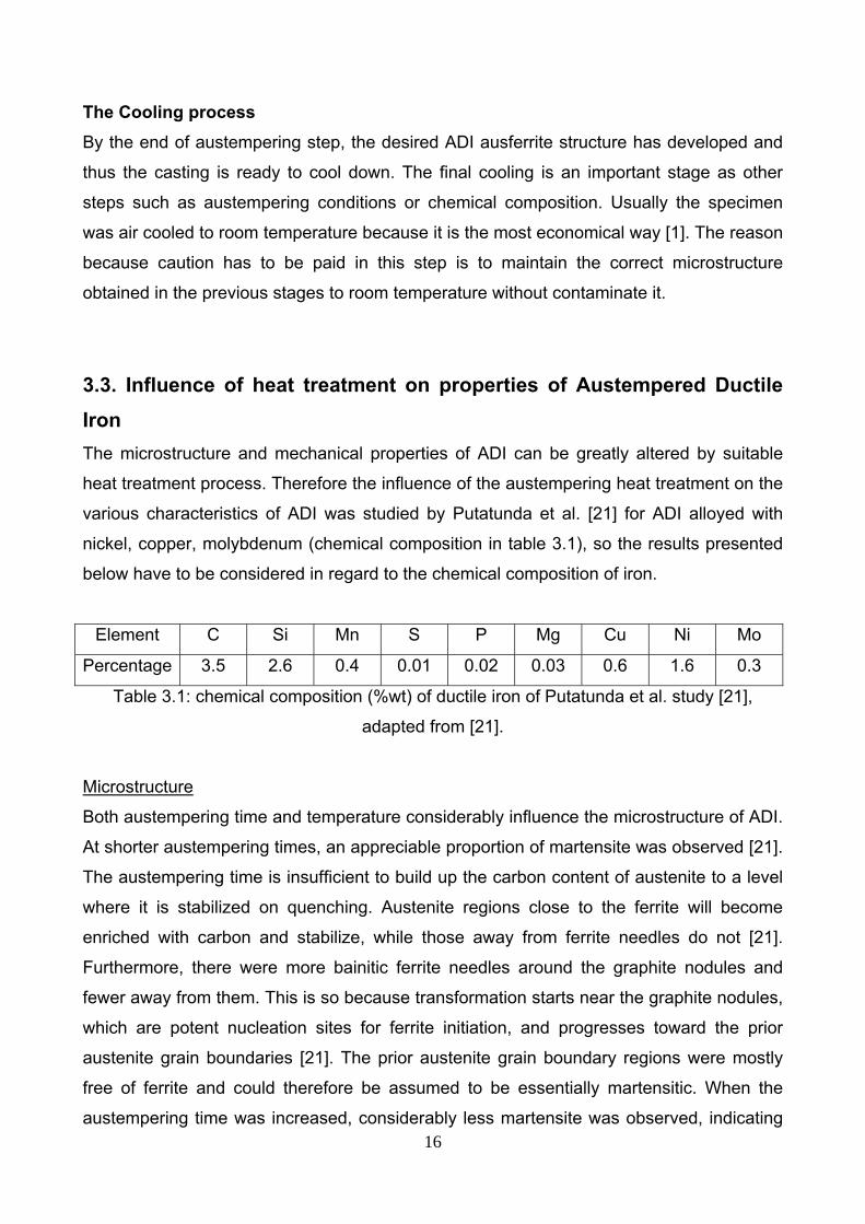
3.3. Influence of heat treatment on properties of Austempered Ductile Iron The microstructure and mechanical properties of ADI can be greatly altered by suitable
heat treatment process. Therefore the influence of the austempering heat treatment on the
various characteristics of ADI was studied by Putatunda et al. [21] for ADI alloyed with
nickel, copper, molybdenum (chemical composition in table 3.1), so the results presented
below have to be considered in regard to the chemical composition of iron.
Element C Si Mn S P Mg Cu Ni Mo
Percentage 3.5 2.6 0.4 0.01 0.02 0.03 0.6 1.6 0.3
Table 3.1: chemical composition (%wt) of ductile iron of Putatunda et al. study [21],
adapted from [21].
Microstructure
Both austempering time and temperature considerably influence the microstructure of ADI.
At shorter austempering times, an appreciable proportion of martensite was observed [21].
The austempering time is insufficient to build up the carbon content of austenite to a level
where it is stabilized on quenching. Austenite regions close to the ferrite will become
enriched with carbon and stabilize, while those away from ferrite needles do not [21].
Furthermore, there were more bainitic ferrite needles around the graphite nodules and
fewer away from them. This is so because transformation starts near the graphite nodules,
which are potent nucleation sites for ferrite initiation, and progresses toward the prior
austenite grain boundaries [21]. The prior austenite grain boundary regions were mostly
free of ferrite and could therefore be assumed to be essentially martensitic. When the
austempering time was increased, considerably less martensite was observed, indicating
17
that bainitic transformation had progressed to a greater extent. At long austempering
times, no martensite was observed [21].
At low austempering temperatures, due to high supercooling, a high nucleation rate results
in a large number of fine ferrite needles [21]. On the other hand, at higher temperatures,
the lower nucleation rate results in fewer ferrite needles, each growing to a larger size. As
the temperature was raised, the amount of austenite increased.
In fact, increasing the austempering temperature, resulted in the coarsening of the acicular
ferrite as well as an increase in the austenite content [21].
Another important microstructural feature is the carbon content of austenite. At the lowest
temperature, it is found that the carbon content rises steadily with austempering time. At
this low temperature, the diffusion rate of carbon is low, and the kinetics of ferrite formation
is fast [21]. Therefore, as ferrite forms, there will be an initial buildup of carbon at the
ferrite/austenite interface. Selecting longer holding times, this carbon may gradually diffuse
into austenite, increasing its carbon content. It should be noted that there is no change in
volume fraction of austenite [21]. Therefore, carbon buildup is not due to the formation of
more ferrite and consequent rejection of carbon into the surrounding austenite [21].
At higher temperatures, faster diffusion rates promote faster buildup of carbon in austenite,
as shown by the rapid increase of carbon content with austempering time. After longer
austempering times, carbon content reaches a saturation value [21]. It should be noted
that the volume fraction of austenite also reached a saturation value around this time. The
saturation value increases with decreasing temperature. This is to be expected as the γ/γ
+ α phase boundary shifts to a higher carbon content of austenite in equilibrium with ferrite
increases with decreasing temperature [21].
The carbon content of retained austenite increases initially, reaches a maximum, and
drops at higher temperatures [21]. At low temperatures, low diffusion rates and fast
kinetics of ferrite formation, means that little carbon diffuses into the austenite. Hence, the
carbon content will be low at lower temperatures [21]. As the temperature rises, more
carbon will find its way into the surrounding austenite from regions transforming to ferrite
due to higher diffusion rates as well as slower kinetics of ferrite formation at decreasing
supercooling. As the temperature is still increased, a stage will be reached when all the

18
carbon from the regions transforming to ferrite will diffuse into the surrounding austenite.
All the carbon in the original austenite at the austenitizing temperature (C0) will now be in
the retained austenite. This is the maximum amount of carbon that can find its way into
retained austenite. The product XγCγ(where Xγ is the volume fraction of retained austenite
and Cγ is the carbon content of the retained austenite) , which gives the total carbon in the
retained austenite, will then have the maximum value and will be equal to C0. Beyond this
temperature, as Xγ increases, Cγ will decrease [21]. Thus, while at lower temperatures
insufficient carbon is reaching the retained austenite, at higher temperatures, no more
carbon is available to enrich the austenite. The optimum is reached at an intermediate
temperature, where the carbon content of austenite will be a maximum [21].
Tensile properties
Low ductility and strength at short austempering times can be attributed to the embrittling
effect due to the presence of martensite at prior austenite grain boundaries [21]. Yield
strength is found to be more sensitive to the austempering time than the tensile strength.
Martensite content decreases as the austempering time increases [21]. Therefore,
strength and ductility increase with increasing time, reaching a plateau after some length
of time. This duration also correspond to the time for attaining maximum retained austenite
content [21].
Both yield strength and tensile strength decrease steadily with rising austempering
temperature. With increasing temperature, bainitic ferrite becomes coarser and the
amount of retained austenite increases. Both these factors lead to a drop in strength but
an increase in ductility [21] (Figure 3.8).

19
250 300 350 400600
800
1000
1200
1400
1600
1800
0
2
4
6
8
10
12
Yield strength Tensile strength
Tens
ile a
nd y
ield
stre
ngth
val
ues
[MP
a]
Austempering temperature [°C]
Elongation
Elo
ngat
ion
(%)
Figure 3.8: influence of austempering temperature on the tensile properties, adapted from
[21].
It has to be observed that the tensile properties of this grade of ADI [21] have to be
considered in regard to the chemical composition of iron. In fact, because of the high
percentage of alloy elements, carbides precipitation can occurs and strongly affect the
mechanical properties of ADI.
Fracture toughness
Similar to the tensile properties, the results about fracture toughness [21] have to be
analyzed in terms of the chemical composition of iron.
At all austempering temperatures, fracture toughness was found to be considerably
influenced by austempering time [21]. The fracture toughness of ADI increased with rising
austempering time until a certain length of time. Beyond that time there was practically no
change in fracture toughness.
The low values at short times can be attributed to the presence of brittle martensite at cell
boundaries. With increasing austempering time, as the austenite content increases,
fracture toughness improves [21].
At a given austempering time, fracture toughness was found to initially increase with
increasing temperature, and thereafter decrease with a further increase in temperature

20
[21] (Figure 3.9). The microstructure can be said to have a profound effect on the fracture
toughness. A lower bainitic structure with fine acicular ferrite imparts better fracture
toughness than an upper bainitic structure with coarse feathery bainitic ferrite [21].
250 300 350 40030
40
50
60
70
Frac
ture
toug
hnes
s [M
Pa*
m1/
2 ]
Austempering temperature [°C] Figure 3.9: influence of austempering temperature on fracture toughness, adapted from
[21].
Some of microstructural features that influence mechanical properties of ADI can be listed
as follows: morphology of bainitic ferrite (whether acicular or feathery), amount of retained
austenite, carbon content of retained austenite, carbide dispersion within austenite or at
austenite/ferrite interface, and dislocation density [21].
Out of these, the retained austenite content is generally regarded as the most important
microstructural feature. The excellent properties of ADI such as good ductility at
comparatively high strength levels, excellent wear resistance, and superior fatigue
properties are believed to be the result of the ability of retained austenite to strain harden
or to transform to martensite when worked [21].

21
10 20 30 40 5010
20
30
40
50
60
70
Frac
ture
toug
hnes
s [M
Pa*m
1/2 ]
Volume fraction of austenite (%) Figure 3.10: influence of austenite content on fracture toughness, adapted from [21].
There is an unmistakable trend of rising fracture toughness with increasing austenite
content, up to a certain high volume fraction with a drop thereafter [21] (Figure 3.10).
Further, some martensite is to be expected due to unstabilized austenite. The presence of
this brittle phase along the prior austenite grain boundaries can initiate crack and also
provide a preferential path for crack propagation [21].
In the absence of this, fracture behaviour is primarily controlled by austenite, as it is the
tougher of the two phases present in the microstructure. Hence, an increasing amount of
retained austenite can result in an increasingly tougher material with consequential
improvement in fracture toughness [21].
The drop in fracture toughness beyond a certain high volume fraction of retained austenite
should be attributed to the change in morphology of ferrite rather than solely to the amount
of austenite [21]. Austenite contents in excess of a certain volume percent are obtained
only when austempering at temperatures higher than 350 °C [21]. At these temperatures,
broad ferrite blades are formed which are free of carbides. At low temperatures, fine
acicular ferrite having heavy dislocation density and fine dispersion of carbides is formed
[21]. In addition, it has been shown that crack initiation in ADI starts with decohesion of
graphite/matrix interface. This raises the stress concentration in the matrix around the
graphite nodules. As a result, extensive plastic deformation occurs in the matrix, which is

22
confined to the ferrite, leading to the formation of microcracks in the ferrite or at the
ferrite/austenite interface [21]. The width of the ferrite plate plays an important role in crack
propagation across the austenite regions. As plastic deformation takes place in ferrite,
dislocation pileups will form within ferrite at the interface. There will be a high stress
concentration at the head of the pileup which, if sufficiently large, can initiate a crack within
austenite. When austempered at higher temperatures, the ferrite blade width will be large,
dislocation pileup will be large, and crack initiation will be easy [21].
A point worth considering at this stage is the possibility of stress-induced martensite
formation, which may provide an easy fracture path, leading to lower fracture toughness.
Because of high carbon content, the Ms temperature is very low, and the austenite is
generally highly stable [21]. On the other hand, austenite formed at higher temperatures
has lower carbon content and, therefore, lower stability. Martensite formation may be
easier in these, as compared to those austempered at lower temperatures. Thus,
formation of stress-induced martensite may be one of the reasons for the lower facture
toughness of ADI with upper bainitic microstructure [21].
Increasing the toughness of retained austenite in the microstructure can also lead to
increased fracture toughness of the ductile iron as a whole [21]. Increasing carbon content
of austenite will increase its toughness, as it will result in greater interaction between
dislocation and carbon atoms. It can be seen that fracture toughness rises with carbon
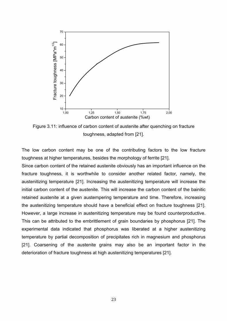
content of austenite (Figure 3.11). Thus, a high carbon content of the retained austenite is
very important in increasing the fracture toughness [21].
23
1,00 1,25 1,50 1,75 2,0010
20
30
40
50
60
70
Frac
ture
toug
hnes
s [M
Pa*
m1/
2 ]
Carbon content of austenite (%wt) Figure 3.11: influence of carbon content of austenite after quenching on fracture
toughness, adapted from [21].
The low carbon content may be one of the contributing factors to the low fracture
toughness at higher temperatures, besides the morphology of ferrite [21].
Since carbon content of the retained austenite obviously has an important influence on the
fracture toughness, it is worthwhile to consider another related factor, namely, the
austenitizing temperature [21]. Increasing the austenitizing temperature will increase the
initial carbon content of the austenite. This will increase the carbon content of the bainitic
retained austenite at a given austempering temperature and time. Therefore, increasing
the austenitizing temperature should have a beneficial effect on fracture toughness [21].
However, a large increase in austenitizing temperature may be found counterproductive.
This can be attributed to the embrittlement of grain boundaries by phosphorus [21]. The
experimental data indicated that phosphorus was liberated at a higher austenitizing
temperature by partial decomposition of precipitates rich in magnesium and phosphorus
[21]. Coarsening of the austenite grains may also be an important factor in the
deterioration of fracture toughness at high austenitizing temperatures [21].
24
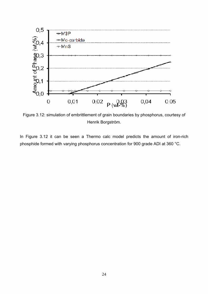
Figure 3.12: simulation of embrittlement of grain boundaries by phosphorus, courtesy of
Henrik Borgström.
In Figure 3.12 it can be seen a Thermo calc model predicts the amount of iron-rich
phosphide formed with varying phosphorus concentration for 900 grade ADI at 360 °C.

25
4. INFLUENCE OF MICROSTRUCTURE ON THE IMPACT PROPERTIES OF AUSTEMPERED DUCTILE IRON
4.1. Effect of austenitization conditions on impact properties of Austempered Ductile Iron Grech et al. [38] investigated about the effect of austenitization conditions on the impact
properties of an alloyed Austempered Ductile Iron with an initial ferritic matrix structure
(containing 1.6% Cu and 1.6% Ni as the main alloying elements, the chemical composition
is listed in table 4.1), more impact tests were carried out on samples of initial ferritic matrix
structure and which had been austenitized at 850, 900, 950, and 1000 °C for 15 to 360
min and austempered at 360 °C for 180 min. The results showed that the austenitization
temperature and time have significant effect on the impact properties of the alloy, which
was attributed to the carbon kinetics [38].
Element C Si Mn S P Mg Ni Cu
Percentage 3.3 2.6 0.35 0.008 0.01 0.04 1.6 1.6
Table 4.1: chemical composition (%wt) of ductile iron of Grech et al. study [38], adapted
from [38].
In a nodular iron with an as-cast pearlitic structure, the graphite spheroids and pearlite
both contribute to the carbon enrichment of the austenite [42]. In a fully ferritic matrix
structure, the graphite nodules are the only source of carbon, and consequently, the
carbon diffusion distances involved during solution treatment may be relatively large [38].
However, some carbon can be attained from the small quantities of spheroidized carbides
present. Consequently, full austenitization requires either very long solution treatment
cycles or a very high carbon diffusion rate, which in turn, calls for higher austenitization
temperatures [38].
At 850 °C, complete austenitization is difficult to achieve: the carbon mobility is rather
slow, and the soaking time selected is not sufficient for complete austenitization to take
place [38]. In fact, irons austenitized for up to 180 minutes still contain pro-eutectoid ferrite
in the austempered structure [38]. The samples austenitized at 900 and 950 °C contain

26
acicular ferrite surrounded by high carbon austenite. The absence of pro-eutectoid ferrite
and martensite can respectively be attributed to full austenitization and to the resulting
stable high carbon austenite [38]. Increasing austenitization temperature increases the
percentage of carbon dissolved in the original austenite, which in turn, decreases the free
energy controlling the transformation of austenite to ferrite and high carbon austenite. The
driving force reduction is responsible for the decrease in the number of ferrite nuclei
formed and the slower growth along the ferrite platelet. Therefore increasing the
austenitization temperature to 1000 °C leads to structures containing a high percentage of
large austenite grains. The center of these regions is low in carbon content and is
therefore relatively unstable. It transforms to martensite as the specimens cool to room
temperature or upon the application of mechanical stress. This has a negative influence on
the impact properties, as shown in Figure 4.1.
To summarize, increasing the austenitization temperature from 850 to 1000 °C eliminates
the pro-eutectoid ferrite and increases the austenite volume fraction. The latter, however,
has a lower carbon content, is less stable, and may transform to martensite on cooling to
room temperature or upon the application of stress.
Specimens austenitized at 850 °C have the highest impact energy value. This has been
attributed to the large volume fraction of the pro-eutectoid ferrite and the morphology of
the acicular ferrite [38].
Specimens solution heat treated at 900 and 950 °C have a fully austempered structure
and relatively high impact energy values [38]. In contrast, specimens austenitized at 1000
°C, have generally lower impact energy values. This is attributed to the higher percentage
of low carbon austenite and the associated martensite [38] (see Figure 4.1).

27
850 900 950 10000
20
40
60
80
100
120
140
Impa
ct e
nerg
y [J
]
Austenitization temperature [°C] Figure 4.1: effect of austenitizing temperature on the impact properties of specimens
austenitized for 180 min, adapted from [38].
The austenitizing time determines the percentage of carbon dissolved in the austenite,
which in turn, affects the rate of austenite transformation during austempering and
therefore, has an influence on the impact energy values attained [38].
The microstructures of samples austenitized for short periods at 850 and 900 °C contain a
considerable volume of pro-eutectoid ferrite [38]. This phase is replaced by ausferrite as
the soaking period extends to 360 minutes at 850 °C or to 60 minutes at 900 °C [38]. In
contrast, the microstructures of specimens austenitized at 950 °C for durations between
15 and 360 min consist generally of acicular ferrite and high carbon austenite [38]. There
are only marginal differences between microstructures of specimens soaked for different
periods. The microstructures of samples austenitized for 15 min at 1000 °C are fully
ausferritic. Increasing the soaking period to 60 min and further results in structures
containing martensite [38].
28
0 60 120 180 240 300 3600
20
40
60
80
100
120
140
Impa
ct e
nerg
y [J
]
Austenitization time [min]
850 °C 900 °C 950 °C 1000 °C
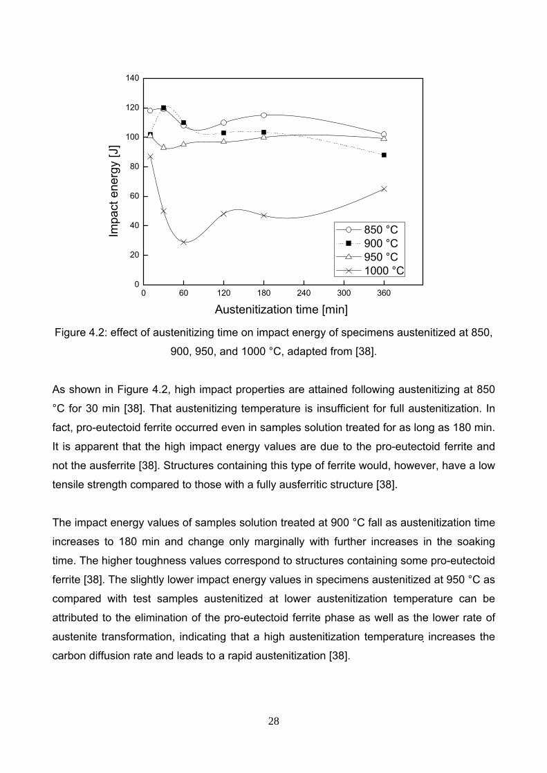
Figure 4.2: effect of austenitizing time on impact energy of specimens austenitized at 850,
900, 950, and 1000 °C, adapted from [38].
As shown in Figure 4.2, high impact properties are attained following austenitizing at 850
°C for 30 min [38]. That austenitizing temperature is insufficient for full austenitization. In
fact, pro-eutectoid ferrite occurred even in samples solution treated for as long as 180 min.
It is apparent that the high impact energy values are due to the pro-eutectoid ferrite and
not the ausferrite [38]. Structures containing this type of ferrite would, however, have a low
tensile strength compared to those with a fully ausferritic structure [38].
The impact energy values of samples solution treated at 900 °C fall as austenitization time
increases to 180 min and change only marginally with further increases in the soaking
time. The higher toughness values correspond to structures containing some pro-eutectoid
ferrite [38]. The slightly lower impact energy values in specimens austenitized at 950 °C as
compared with test samples austenitized at lower austenitization temperature can be
attributed to the elimination of the pro-eutectoid ferrite phase as well as the lower rate of
austenite transformation, indicating that a high austenitization temperature increases the
carbon diffusion rate and leads to a rapid austenitization [38].

29
The toughness falls rapidly as the solution treatment time increases for samples
austenitized at 1000 °C. The high impact energy values can be attributed to the low
content of dissolved carbon in the austenite and, consequently, the relatively high driving
force controlling the austempering reaction [38]. Increasing the soaking period to 60 min
increases the dissolved carbon and results in a coarser structure containing martensite
[38]. It is not clear, however, why soaking for more than 60 min gives rise to a recovery in
impact energy values [38].
In conclusion, including both austenitization temperature and time parameters, it has been
shown that, for the Cu-Ni alloy investigated, optimum impact energy values are attained
when austenitization is carried out between 900 and 950 °C for 120 to 180 minutes [38].
These austenitization conditions are such as to eliminate the pro-eutectoid phase but at
the same time do not reduce substantially the rate of austenite transformation;
consequently, these optimum conditions do not promote the formation of martensite [38].
4.2. Effect of austempering conditions on impact properties of Austempered Ductile Iron An investigation about the austempering study of properties of alloyed ductile iron [39]
shows the behaviour of impact properties when the austempering conditions (time and
temperature) have been changed. In that work [39], specimens austenitized in a protective
argon atmosphere at 900 °C for 2 hours were rapidly transferred to a salt bath at
austempering temperatures 300, 350, and 400 °C, held for 1, 2, 3 and 4 hours and then air
cooled to room temperature, the chemical composition is listed in table 4.2.
Element C Si S Mn P Mg Cr Ni Mo
Percentage 3.6 2.5 0.01 0.3 0.04 0.05 0.05 0.95 0.5
Table 4.2: chemical composition (%wt) of ductile iron of study of properties of alloyed
ductile iron [39], adapted from [39].
Mechanical properties (strength, elongation and impact energy) strongly depend on
amounts of acicular ferrite and retained austenite [39]. Time and temperature of isothermal
transformation during austempering treatment have a marked influence on the relative
amount of retained austenite (Figure 4.3) [39].

30
0,5 1,0 1,5 2,0 2,5 3,0 3,5 4,0
0
5
10
15
20
25
Ret
aine
d au
sten
ite (%
)
Austempering time [h]
300 °C 350 °C 400 °C
Figure 4.3: effect of austempering time on the volume fraction of retained austenite at
different austempering temperatures, adapted from [39].
From the shape of curves in Figure 4.3 it is apparent that two stages are involved in the
isothermal transformation, as described in the previous paragraphs. In the Stage 1 (times
less than 2 h) the amount of retained austenite increases with time. This may be explained
taking into account that the transformation to bainite was not completed [39]. It is well
documented [40] that austenitic regions having low silicon and high carbon concentration,
e.g., regions between graphite nodules, will not undergo transformation (to bainitic ferrite
and retained austenite) during short time of austempering, so during the subsequent
cooling from austempering to room temperature the formation of martensite cannot be
prevented. With somewhat longer austempering time the amount of retained austenite
increases reaching maximum after 2 h. However, after 2 h the amount of retained
austenite decreases, indicating the start of the Stage 2 of austempering reaction when
retained austenite decomposes to bainitic ferrite and carbide [39]. At 400 °C this decrease
is more pronounced and is associated with the decomposition of austenite to ferrite and
carbide [41].
Low values of impact energy (Figure 4.4) at short austempering times are connected with
the significant amount of brittle fracture caused by the presence of martensite in the
structure [39]. With longer time martensite disappears in the structure, whereas the
amount of bainitic ferrite and retained austenite increases resulting with a maximum of

31
impact energy after 2 h of austempering [39]. With further increase of time a decrease in
impact energy occurs. This decrease is evident especially at 400 °C: the low values of
impact energy correspond to a fall of the amount of retained austenite at longer
austempering time [39].
0,5 1,0 1,5 2,0 2,5 3,0 3,5 4,0
20
30
40
50
60
70
80
90
100
110
120
Impa
ct e
nerg
y [J
]
Austempering time [h]
300 °C 350 °C 400 °C
Figure 4.4: the effect of austempering time on impact energy at different austempering
temperatures, adapted from [39].
The variation of impact energy after 2 h of holding at different austempering temperatures
is shown in Figure 4.5. As austempering temperature increases martensite disappears
from the structure and the amount of retained austenite increases [39]. These changes
result in reduced strength but increase of impact energy as the amount of retained
austenite increases: values of impact energy show maximum at 350 °C which coincides
with the highest amount of retained austenite (see Figure 4.5) [39].

32
300 320 340 360 380 400
60
70
80
90
100
110
Impa
ct e
nerg
y [J
]
Austempering temperature [°C] Figure 4.5: effect of austempering temperature on impact energy after 2 h of
austempering, adapted from [39].
According to the results of the study the optimal processing window was established for
austempering at 350 °C 2 h [39]. The obtained microstructure consisting of acicular ferrite
and retained austenite yield the best combination of mechanical properties (tensile
strength, elongation and impact energy) [39]. Alloying with copper improves elongation
and impact energy, but decrease strength of ADI [39].
4.3. Effect of alloy elements segregation on impact properties of Austempered Ductile Iron The effect of segregation of alloying elements on the phase transformation of ductile iron
during austempering was investigated by Lin et al. [43]. Four heats, each containing
0.4%Mn, 1%Cu, 1.5%Ni, or 0.4%Mo (%wt) separately, were melted.
Segregation was found with those positive segregating elements, Mn and Mo, and those
negative segregating elements, Si, Cu, and Ni [43]. The segregation of Mo is more
significant than Mn. The segregation of Cu is more than Ni, and that of Ni is more than Si
[43]. The ability of Cu to hinder carbon diffusion at the graphite-austenite interface during
the eutectoid transformation results in pearlite being present [43]. Other alloys exhibit
substantial ferrite in the as-cast structure with pearlite relegated to near the intercellular
regions [43].

33
Between the time of finishing the first stage and beginning the second stage of bainite
reaction in ductile irons, there is a significant “processing window” for austempering to
obtain optimum mechanical properties [43]. The austempering temperature is a critical
factor affecting the processing window, which is relatively narrow for austempering of 400
°C (falling within approximately 103 to 5x10³ seconds) but wider at 350 °C (approximately
2x10³ to 105 seconds) [43].
The microsegregation of alloying elements leads to a reduction in the processing window.
The greater the degree of segregation, the less will be the span of the processing window
[43]. Due to this ratio, the difficulty of controlling the process of austempering of ductile
irons is increased.
Impact toughness is significantly affected by the segregation [43]. The impact strength for
the specimens with less segregation is greater than for those with greater segregation
[43]. The microstructures of Ni, Cu, and Mn alloys in each austempered condition show
completion of the first stage of bainite reaction, and the impact values of these three alloys
in the same diameter are not significantly different [43].
Mo has the most extreme segregating tendency of all alloying elements in this study, and it
retards the bainite reaction and causes microshrinkage porosity in the intercellular regions.
Consequently, the Mo-alloyed irons austempered at 350 °C and 400 °C have the lowest
impact strength among all alloys [43].

34
5. INFLUENCE OF MICROSTRUCTURE ON THE FATIGUE PROPERTIES OF AUSTEMPERED DUCTILE IRON
Many different mechanical failure modes exist in all fields of engineering. These failures
can occur in simple, complex, inexpensive, or expensive components or structures. Failure
due to fatigue is multidisciplinary and is the most common cause of mechanical failure.
Even though the number of mechanical failures compared to successes is minimal, the
cost in lives, injuries, and dollars is too large [33]. Proper fatigue design includes
synthesis, analysis and testing are to the real product and its usage, the greater
confidence in the engineering results.
Applicable fatigue behaviour and fatigue design principles have been formulated for nearly
150 years since the time of Wöhler’s early work [33]. These principles have been
developed, used, and tested by engineers and scientists in all disciplines and in many
countries.
The term “fatigue” refers to gradual degradation and eventual failure that occur under
loads which vary with time, and which are, most of the time, lower than the yield strength
of the specimen, component or structure concerned [31]. These loads are cycling in
nature, but the cycles are not necessarily all of the same size or clearly discernible. A
fatigue load in which individual cycles can be distinguished is usually called a cyclic load
[31].
If a specimen is subjected to a cyclic load, a fatigue crack nucleus can be initiated on a
microscopically small scale, followed by crack growth to a macroscopic size, and finally
specimen failure in the last cycle of the fatigue life [32].
Understanding of the fatigue mechanism is essential for considering various technical
conditions which affect fatigue life and fatigue crack growth, such as the material surface
quality, residual stress, and environmental influence. This knowledge is essential for the
analysis of fatigue properties of an engineering structure. Fatigue prediction methods can
only be evaluated if fatigue is understood as a crack initiation process followed by a crack
growth period [32].
The fatigue life is usually split into a crack initiation period and a crack growth period [32].
The initiation period is supposed to include formation of microcrack and microcrack
growth, but the fatigue cracks are still too small to be visible by the unaided eye. In the

35
second period, the crack is growing until complete failure. It is technically significant to
consider the crack initiation and crack growth periods separately because several practical
conditions have a large influence on the crack initiation period, but a limited influence or no
influence at all on the crack growth period [32].
A constant amplitude fatigue loading (or constant amplitude loading) is a fatigue loading in
which all the load cycles are identical [31] (Figure 5.1). A cycle is the smallest unit of the
stress history which repeat exactly. Cycles are often, but not always, sinusoidal [31].
There are several symbols in the fatigue theory: σa is the amplitude, σm is the mean stress,
σmax is the maximum stress in the load cycle, σmin is the minimum stress in the load cycle.
Mathematically a load cycle (or stress cycle) is expressed as σm ± σa. Compressive
stesses are taken as negative.
The stress range is , and the stress ratio, .
Figure 5.1: notation for constant amplitude fatigue loading, adapted from [31].

36
Conventionally, results are presented as S/N curves (Figure 5.2). These are plots of
Alternating stress versus Number of cycles to failure, with an appropriate curve fitted
through the individual data points (sometimes, stress range is used) [31]. Failure is usually
defined as the separation of a specimen into two parts, but other definitions are sometimes
used. For example, loss of a specified amount of stiffness or the appearance of a crack of
a specified size. S/N curves are sometimes called Wöhler curves [31]. The number of
cycles to failure is sometimes called the life or the endurance. It is usually plotted on a
logarithmic scale, but alternating stress may be plotted on either a linear or a logarithmic
scale [31]. As used to be conventional (Frost et al. 1974) these S/N curves are for
endurances of less than 108 cycles. The region where failure takes place in less than
about 104 cycles is called low cycle fatigue, and the region for longer endurances high
cycle fatigue [31]. In some cases the tests were stopped before 108 cycles, when the
specimens were still unbroken, and suggested that the line through the points in the S/N
curves became horizontal. When it occurs, the stress corresponding to the horizontal line
is called the fatigue limit [31].
log σ a
log N Figure 5.2: typical S/N curve, adapted from [31].
Crack surface surfaces are stress-free boundaries adjacent to the crack tip and therefore
dominate the distribution of stresses in that area [31]. Remote boundaries and loading
forces affect only the intensity of the stress field at the crack tip [31]. These fields can be
divided into three types corresponding to the three basic modes of crack surface

37
displacement, and are conventionally characterized by the stress intensity factor K (with
subscript I, II, III to denote the mode) [31]. K has the dimensions (stress) x (length)1/2 and
is a function of the specimen dimensions and loading conditions [31]. Conventionally, K is
expressed in MPa m1/2 [31]. In general, the opening mode (I) intensity factor is given by
[31]:
where is the tensile stress perpendicular to the crack, is the crack length and is a
factor, of the order of unity, which depends on geometry and loading conditions [31].
In the analysis of fatigue crack growth data, the fatigue cycle is usually described by ΔK =
(Kmax - Kmin), where Kmax and Kmin are the maximum and the minimum values of KI during
the fatigue cycle [31]. It has been shown that ΔK rather that Kmax has the major influence
on fatigue crack growth and that, if ΔK is constant, the fatigue crack growth rate is
constant [31]. For many materials, subjected to tensile loading cycle, the rate of fatigue
crack growth can be expressed by the equation [31], also known as Paris law:
where is the number of cycles, is a material constant and is an exponent, usually
about 3 or 4 for steel, and represents the slope of the curve when the data are plotted
log(da/dN) against log(ΔK).
A crack will not grow under cycling loading unless the range of stress intensity factor
during a fatigue cycle exceeds a critical value ΔKth [31]. This value of stress intensity factor
is called Threshold value and if ΔK is below a certain Threshold value, fatigue crack
growth does not occur [31]. It can be obtained by carrying out fatigue tests on precracked
plates and plotting the results as ΔK against crack growth rate (da/dN). The resulting
curves were similar in shape to conventional S/N curves, ΔKth being the value of ΔK at
which a curve becomes parallel to abscissa (see Figure 5.3). The parameter ΔKth
therefore, is analogous to the fatigue limit [31]. Furthermore, the slope of the different
curves are linked by the following relation:

38
Figure 5.3: Wohler and FCGR curves.
5.1. High Cycle Fatigue of Austempered Ductile Iron In the study of Lin at al. [12] rotary bending tests with stress ratio R equal to -1 were
conducted on a number of different grades of Austempered Ductile Iron (designated as A,
B, C, and D, the different chemical compositions and nodule parameters are given in table
5.1). The ADI heat-treat cycle consists of an austenitization in a salt bath at 900 °C for 1.5-
2 h and 2 different austempering condition to obtain different mechanical properties related
to changed microstructure. The first austempering, that generated the optimum strength
(with a optimum combination of ultimate tensile strength, yield strength and hardness),
was carried out at 300 °C: at this transformation temperature it was observed that the
ferrite laths are finer and closer together. The second austempering, that generated the
optimum strength (with a maximum value of impact energy), was carried out at 360 °C: at
this temperature the ferrite laths become coarser and shorter. Chemical composition and
nodule data of ductile irons are showed in table 5.1.

39
C Si Mn P S Mg Cu Ni Mo
Nodule
count
(n°/mm-2)
Nodule
radius
(μm)
Nodularity
(%)
A 3.6 2.3 0.1 0.04 0.01 0.04 0.5 0.5 - ~ 100 25 ~ 80
B 3.6 2.5 0.2 0.02 0.01 0.04 0.5 0.4 - ~ 110 20 ~ 90
C 3.6 2.6 0.2 0.02 0.01 0.05 0.4 0.4 - ~ 150 17 ~ 90
D 3.6 2.6 0.3 0.05 0.01 0.04 0.5 0.4 0.2 ~ 200 12 ~ 90
Table 5.1: chemical composition (%wt) and nodule data of ductile irons utilized in Lin’s
study [12], adapted from [12].
The effects of austempering temperatures, nodularity, nodule count and amount of
retained austenite were discussed in that study [12] and were found the results presented
below.
104 105 106 107 108100
150
200
250
300
350
400
450
500 As-cast ADI Lower Taustempering
ADI Higher Taustempering
Stre
ss [M
Pa]
Cycles to failure Figure 5.4: example of S/N curves for HCF obtained for as-cast iron and ADI treated at
two different temperature to obtain optimum strength and toughness, adapted from [12].
The fatigue limit is not proportional to its tensile strength, but is related to its toughness
and retained austenite content [12]. In general, ADI was achieved with austempering
treatment that gave optimum toughness and larger amounts of retained austenite, which
has a better HCF performance [12]. In addition, the fatigue ratio of ADI increased with a
40
decrease in tensile strength but with an increase in toughness and retained austenite
content [12].
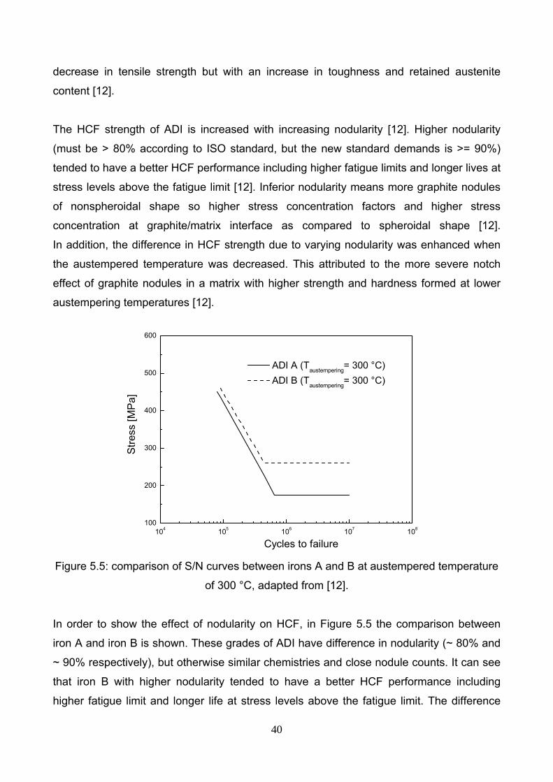
The HCF strength of ADI is increased with increasing nodularity [12]. Higher nodularity
(must be > 80% according to ISO standard, but the new standard demands is >= 90%)
tended to have a better HCF performance including higher fatigue limits and longer lives at
stress levels above the fatigue limit [12]. Inferior nodularity means more graphite nodules
of nonspheroidal shape so higher stress concentration factors and higher stress
concentration at graphite/matrix interface as compared to spheroidal shape [12].
In addition, the difference in HCF strength due to varying nodularity was enhanced when
the austempered temperature was decreased. This attributed to the more severe notch
effect of graphite nodules in a matrix with higher strength and hardness formed at lower
austempering temperatures [12].
104 105 106 107 108100
200
300
400
500
600
ADI A (Taustempering= 300 °C) ADI B (Taustempering= 300 °C)
Stre
ss [M
Pa]
Cycles to failure Figure 5.5: comparison of S/N curves between irons A and B at austempered temperature
of 300 °C, adapted from [12].
In order to show the effect of nodularity on HCF, in Figure 5.5 the comparison between
iron A and iron B is shown. These grades of ADI have difference in nodularity (~ 80% and
~ 90% respectively), but otherwise similar chemistries and close nodule counts. It can see
that iron B with higher nodularity tended to have a better HCF performance including
higher fatigue limit and longer life at stress levels above the fatigue limit. The difference

41
between the two HCF behaviours isn’t strongly marked at low cycles, but it increases
when the stress levels are close to the fatigue limit, where it shifts to lower value for iron
with less nodularity.
The HCF resistance of ADI was improved when the nodule count increased, in particular
at austempered temperatures for optimum toughness [12]. Therefore, ADI with a greater
nodule count or a smaller nodule size exhibits a better HCF behaviour [12]. The more
pronounced beneficial effect of a large nodule count on the HCF properties of ADI for the
matrix structure with optimum toughness may be explained by the difference in the
amounts of retained austenite. Greater amounts of retained austenite can create more
barriers for fatigue crack growth and extend life [12].
The better HCF strength is suggested not to be attributed exclusively to the advantage of
greater nodule count because this improvement was lost in LCF behaviour [12, 13]. It is
probably related to the volume fraction, size and distribution of retained austenite in matrix
[12]. It may be attributed to the larger amounts of retained austenite and a greater fraction
of retained austenite in low concentration of carbon [12]. This low carbon austenite is more
likely to transform to martensite under plastic deformation (stress-induced martensitic
transformation) than carbon-enriched stable austenite, resulting in a greater fatigue crack
growth resistance. The amounts of retained austenite increased with increasing the
austempering temperature so a larger fraction of retained austenite would undergo
martensitic transformation under plastic deformation. Stress-induced martensitic
transformation of austenite occurred locally in the plastic zone ahead of the crack so as to
relax the stress concentration at the crack tip. The accompanying volume change also
encouraged plastically induced crack closure to occur, reducing the fatigue crack growth
rate and increasing fracture toughness [12].

42
104 105 106 107 108100
200
300
400
500
600
ADI B (Taustempering = ~ 360 °C) ADI D (Taustempering = ~ 360 °C)
Stre
ss [M
Pa]
Cycles to failure Figure 5.6: comparison of S/N curves between ductile irons B and D at austempered
temperature of 360 °C, adapted from [12].
In Figure 5.6 the different behaviour between ductile iron B and D is shown. The chemical
composition of iron D is close to that of iron B except for the addition of 0.2% of Mo and
greater amounts of Mn. In addition, iron D has a nodule count of 200 nodules/mm-2, more
than the 110 nodules/mm-2 of iron B and also the amount of retained austenite is larger in
D. ADI-B exhibits a much better HCF performance than ADI-B. The better HCF strength is
not to be attributed exclusively to the advantage of greater nodule count as described
above, because this improvement was lost in LCF behaviour [13]. So it can be concluded,
as shown in Figure 5.6, that the effect of volume fraction, size and distribution of retained
austenite in matrix strongly affect the HCF performance of ADI.
Large graphite nodules, inclusions, micro shrinkage pores, and irregularly shaped graphite
clusters at or near the surfaces of the HCF specimens are the typical crack initiation [12].
Failure usually begin with extensive nodule decohesion from the matrix followed by
localized plastic deformation in the matrix resulting in microcracks extending from many
graphite nodules [12]. Decohesion is due to mismatch in mechanical properties between
graphite and matrix structure and take place at the graphite/matrix interface at low level of
strain. At the higher values of strain, localized plastic deformation and microcracking occur
to relieve the stress concentrations caused by the graphite nodule voids [12].

43
ADI´s fatigue crack path largely depends on the location of the next nodule ahead of the
crack tip [12]. It usually goes through the areas with highly distributed graphite nodules,
which provide the least-energy path to link graphite nodules. For the crack path between
two neighbouring nodules, fatigue crack was observed to grow along the austenite/ferrite
interfaces or cut through the ferrite laths [12].
Results of another study about the high-cycle fatigue of ADI [16] show that the fatigue limit
in ADI is controlled by a crack arrest. Ausferrite packet boundaries act as barriers for
microstructurally-small cracks due to a requirement for the first stage growth in the
ausferrite matrix. The strength of the barrier depends on the relative orientations of the
microstructure at the boundary.
5.2. Low Cycle Fatigue of Austempered Ductile Iron Lin et al. also investigated the low-cycle fatigue (LCF) properties of ADI [13]. In this work,
unlike the case for HCF analysis, ADIs were tested under uniaxial condition under strain-
control, constant amplitude, totally reversed loading (R = -1).
Heat treatment was consisted of first austenitization and austempering at two different
temperatures to obtain two different microstructures. The chemical composition and
nodule data of the different grades of iron were the same as the previous paragraph (table
5.1).
The austenitization was carried out in a salt bath at 900 °C for 1.5-2 h and 2 austempering
treatments for each ductile iron were conducted to generate ADIs with two different
optimal properties. For the first austempering condition, that generate the optimum
strength (with a optimum combination of ultimate tensile strength, yield strength and
hardness), the austempering treatment was carried out at 300 °C. At this transformation
temperature was observed that the ferrite laths are finer and closer together. The second
austempering condition instead, generate the optimum strength (with a maximum value of
impact energy). The austempering temperature was chosen at 360 °C: at that
transformation temperature the ferrite laths become coarser and shorter. The outcomes of
study [13] are described below.

44
101 102 103 104 1050,1
0,5
1
As-cast ADI Lower Taustempering
ADI Higher Taustempering
Stra
in A
mpl
itude
(%)
Cycles to failure Figure 5.7: example of strain-life curves for LCF for as-cast iron and ADI treated at two
different temperature to obtain optimum strength and toughness, adapted from [13].
As-cast ductile irons exhibited cycling hardening while austempered ductile irons showed
cycling softening [13]. Ductile irons with initially hard and strong matrix structures will
generally cyclically soften, and those with initially soft matrix structures will cyclically
harden [13]. Such cyclic softening phenomenon was attributed to the continuous
development of damage such as cracking and decohesion of graphite nodules at the
matrix interface [13]. Whether a ductile iron austempered with the optimum strength or
toughness would exhibit the optimum LCF performance may be related to graphite
morphology [13].
In ADIs with a large nodule size, the voids formed by decohesion of graphite nodules
would be larger as well as the induced stress concentration fields [13]. More deformation
would take place in the matrix due to the larger areas under higher stress and lead to
formation of more microcracks extending from the graphite nodules. So the austempered
ductile irons with greater toughness would delay the propagation and link-up of
microcracks and exhibit a longer LCF life [13].
On the other hand, ADIs with a smaller nodule size displayed smaller stress concentration
fields and less induced deformation [13]. The formation of microcracks originated from the
nodules was suppressed despite of the crack path between graphite nodules being
shorter. Therefore, it would be more difficult to generate microcracks in ADIs with higher
strength; so ADIs austempered at lower temperatures show higher LCF strength [13].

45
It was found that the LCF strength of ADI increased with increasing nodularity [13]. At both
lower and higher austempered temperatures, ductile irons with better nodularity tended to
have a longer fatigue life, in particular at small strain levels. Higher nodularity (> 80%)
means more graphite nodules of spheroidal shape and lower stress concentration factors
as compared to other nonspheroidal shapes [13]. This develops a less stress
concentration at graphite/matrix interface. Therefore, increasing graphite nodularity can
improve ADI’s LCF strength [13].
It was found that the LCF strength of ADI increased with increasing nodule count [13]. For
ductile irons with higher nodule counts, austempering for optimum strength generated the
best LCF behaviour while the best LCF performance could be obtained by austempering
for optimum toughness for ductile irons with lower (< 100 n°/mm2) nodule count [13].
It was found that, as described above, an increase in nodule count could improve the LCF
life of ADI for a given chemical composition. However, this improvement may be lost due
to the effect of morphology of retained austenite [13]. A larger fraction of retained austenite
that is not rich in carbon content, would transform to martensite under plastic deformation.
Although the stress-induced martensitic transformation may have a beneficial effect on the
HCF behaviour of ADI under rotary bending as reported in the previous paragraph, this is
not the case for LCF behaviour of ADI under axial loading [13]. Since LCF test tests were
conducted under axial cycling loading at very high stress levels, plastic deformation took
place in the whole gage sections of the specimens. Consequently, larger amounts of
stress-induced martensitic transformation might occur throughout the entire gage section
of specimens, resulting in the embrittlement of the matrix, premature initiation of
microcracks, and reduction of toughness and fatigue crack growth resistance [13]. In other
words, ADI with larger amounts of austenite in low carbon concentration has a worse LCF
performance under axial loading [13].
Fatigue cracks initiated not only from graphite nodules but also from casting defects. The
fractures origins are identical to those observed in the HCF specimens [13].
The LCF failure in as-cast and austempered ductile irons began with extensive nodule
decohesion from the matrix followed by localized plastic deformation in the matrix resulting
in formation of microcracks emanating from many graphite nodules [13]. Selected

46
microcracks link up to form larger microcracks, which in turn can link up to initiate a
primary crack or extend a propagating crack resulting in the final failure [13].
The fatigue crack propagation path depends strongly on the location of the next graphite
nodule ahead of the crack tip, but in general is perpendicular to the loading direction [13].
The crack path between two graphite nodules is along the least-energy path which is often
the interfaces between ferrite and austenite but is also influenced by ferrite-lath´s
orientation relative to loading direction and by the presence of precipitated carbides which
can change the least-energy path [13].
5.3. Low Cycle Fatigue of Austempered Ductile Irons at various strain ratios In the study of Lin et al. [14], uniaxial LCF tests were conducted under strain-control with
three strain ratios, R = -1, 0, 0.5 to investigate the low-cycle fatigue properties of ADI at
various strain ratios. Two types of austempering treatments were applied to the base irons
so as to investigate the response of different ausferritic structures. Chemical composition
of ADIs tested is showed in table 5.2.
Element C Si Mn P S Mg Cu Fe Bi
Percentage 3.6 2.5 0.2 0.03 0.01 0.04 0.6 bal. 40 ppm
Table 5.2: chemical composition (%wt) of ADIs tested in Lin et al. work [14], adapted from
[14].
Test specimens were first austenitized in salt bath at 900 °C for 1.5 h after which they
were either quenched in salt bath at 300 °C and 3 h for a higher strength value, or at 360
°C and 2 h for greater toughness; they were then cooled in forced air. As described above,
a change from a fine to coarse ausferritic matrix structure can be seen as the
austempering temperature increases. The greater toughness and ductility obtained at 360
°C result from the larger amounts of retained austenite present in the matrix [14].
For a given austempering treatment, the LCF life of ADI was decreased with an increase
in strain ratio due to the intensifying mean stress effects [14] (Figure 5.8). The degree of

47
mean stress influence on ADI’s LCF behaviour appeared to be function of austempering
treatment and in turn the ausferritic matrix structure [14].
Figure 5.8: strain-life curves of ADIs in different strain ratios R, adapted from [14].
In completely-reversed LCF tests, ADI austempered at 300 °C provided more fatigue
resistance than did those austempered at 360 °C due to less extent of martensitic
transformation of unstable retained austenite [14]. The superiority of ADIs austempered at
300 °C to those austempered at 360 °C is related to the amounts and stability of the
retained austenite in ausferritic matrix. ADIs with a greater volume fraction of retained
austenite, particularly the unstable, blocky type, exhibited less LCF resistance due to the
higher probability of plasticity-induced martensitic transformation under large magnitude of
uniaxial loading [14]. Since LCF tests were conducted under uniaxial cycling loading at
very high strain/stress level, plastic deformation took place in the whole gage sections of
the specimens. Consequently, a greater extent of plasticity-induced martensitic
transformation might occur during LCF test throughout the entire gage sections of ADI
102 103 104 1050,1
0,5
1
360 °C, 2h 300 °C, 3h
Stra
in A
mpl
itude
(%)
Cycles to failure
R = -1
102 103 104 1050,1
0,5
1
360 °C, 2h 300 °C, 3h
Stra
in A
mpl
itude
(%)
Cycles to failure
R = 0
102 103 104 1050.1
0.5
1
360 °C, 2h 300 °C, 3h
Stra
in A
mpl
itude
(%)
Cycles to failure
R = 0.5

48
specimens austempered at 360 °C, resulting in non-uniform, localized embrittlement of the
matrix, premature initiation of microcracks, and reduction of toughness and fatigue crack
growth resistance [14]. Therefore, the plasticity-induced martensitic transformation of
unstable retained austenite is a detrimental effect on the LCF behaviour of ADI under
completely-reversed uniaxial loading [14].
For the completely-reversed LCF tests, the difference in the mean stress levels between
the two austempering conditions is not significant such that the LCF performance is mostly
influenced by the effects of plasticity-induced transformation of unstable retained austenite
to martensite [14]. For LCF tests at R = 0 and 0.5, the tensile mean stress levels are
considerably higher in ADIs austempered at 300 °C than in those 360 °C ones leading to
the shorter fatigue lives in ADIs austempered at 300 °C [14]. The degree of difference in
the tensile mean stress level between two austempering treatments is extended as strain
ratio and strain amplitude increases [14].
For each austempering treatment the fatigue life is significantly reduced with an increase
in strain ratio, given a strain amplitude [14]. This can be attributed to the presence of
tensile mean stresses for LCF tests at R = 0 and 0.5. The degree of reducing fatigue life
by a larger strain ratio is more extensive for ADIs austempered at 300 °C indicating this
grade of ADI is more sensitive to mean stress effects on LCF resistance [14] (Figure 5.9).
Figure 5.9: comparison of strain-life curves of ADIs with different strain ratios at two
austempering conditions, adapted from [14].
102 103 104 1050,1
0,5
1
R = -1 R = 0 R = 0.5
Stra
in A
mpl
itude
(%)
Cycles to failure
300 °C, 3h
102 103 104 1050,1
0,5
1
R = -1 R = 0 R = 0.5
Stra
in A
mpl
itude
(%)
Cycles to failure
360 °C, 2h

49
5.4. Mechanism of fatigue crack growth in Austempered Ductile Iron
Fractographic analysis of fatigue fracture surfaces at threshold show striations typical of a
ductile fracture mechanism [15]. In the proportional growth regime striations and cleavage
planes are shown, revealing a quasi-cleavage failure mode [15]. The effect of matrix
microstructure is minor, and can be attributed to the different crack closure contribution of
each microstructure [15].
Figure 5.10: typical fracture surface in ADI.
The main propagation mechanism is given by small cracks emanating from nodules and
growing towards the principal crack [15]. In other words, propagation of the main crack is
partly due to the initiation and growth backwards of small cracks started at surface
irregularities of the graphite nodules [15]. Initiation of these cracks is apparently activated
by the stress raise produced when the tip of the main crack is at a sufficiently short
distance from the nodule. These small cracks eventually coalesce with the main crack
front, which continues to grow in the normal way until a new nodule is reached [15]. It is
important to take into account that several nodules can be involved in the growth process
at the different portions of the crack front, so that the average growth rate is affected by
the size, shape and distribution of graphite nodules [15], a typical fracture surface due to
fatigue is shown in Figure 5.10.

50
In the same study [15], Threshold and propagation fatigue regimes are analyzed for two
commercial low alloy ductile cast irons, both austenitized at 900 °C for 2 h and then
austempered at different temperatures and times. Two different casts were used: Cast 1
(0,28% Mn, 0,90% Cu, 0,53% Ni) was used for fatigue threshold measurements (batches
named A-D), and Cast 2 (0,20% Mn, 1,33% Cu, 1,03% Ni) was used for fatigue
propagation tests (batches named F-I). Samples were machined from ‘Y’ blocks of
thickness 1 inch (cast 1), 1/2 inch. (cast 2a) and 3 inch. (cast 2b) respectively.
Crack growth rates and threshold stress intensity ranges ΔKth were determined according
to ASTM E-647. The results achieved are listed in tables 5.3 and 5.4 [15].
Batch Austempering temperature
[°C]
Austempering time
[min] ΔKth [MPa√m]
A 260 120 4,77
B 290 120 5,18
C 320 90 5,61
D 360 90 6,35
Table 5.3: threshold stress intensity ranges for different heat treatment, adapted from [15].
Batch Austempering
temperature [°C]
Austempering
time [min] C m
F (2a) 260 120 8,18 x 10⁻¹² 2,92
G (2b) 260 120 2,39 x 10⁻¹¹ 2,66
H (2a) 360 90 1,16 x 10⁻¹¹ 2,91
I (2b) 360 90 6,79 x 10⁻¹² 2,95
Table 5.4: values of m and C for different heat treatment, adapted from [15].

51
5.5. Influence of heat treatment on fatigue crack growth of Austempered Ductile Iron Fatigue crack growth rates (FCGRs) of ADIs were compared with those of the as-cast DI
with a bull’s eye microstructure to examine the influence of austempering treatment on the
FCG behaviour of DI dependent on the stress intensity range (ΔK) and load ratios (R) in
Lin et al. study [19]. Chemical composition of iron is showed in table 5.5.
Element C Si Ni Cu Mn Mo Mg P S
Percentage 3.5 2.3 0.5 0.4 0.2 0.2 0.04 0.03 0.01
Table 5.5: chemical composition (%wt) of iron in Lin’s study [19], adapted from [19].
Influence of microstructure:
The FCG behaviour clearly shows a microstructural dependence as interactions of the
FCGR curves for the as-cast DI and ADIs occurred at certain transition ΔK values [19].
For a given load ratio, the as-cast DI with a bull’s eye matrix structure exhibited the lowest
FCGR in the low ΔK regime [19]. In the high ΔK region, the ADIs with ausferritic matrix
structures provided more or comparable FCG resistance as compared to the as-cast bull’s
eye microstructure depending on the R value [19]. In addition, ADI austempered at higher
temperature with a coarser ausferrite matrix structure and greater amount of retained
austenite exhibited lower FCGRs than did ADI austempered at lower temperature with a
finer ausferritic microstructure and lower volume fraction of retained austenite [19] (see
Figure 5.11).

52
1010-6
10-5
10-4
10-3
10-2
As-cast ADI Taustempering= 300 °C, 3h ADI Taustempering= 360 °C, 2h
Fatig
ue C
rack
Gro
wth
Rat
e [m
m/c
ycle
]
Stress Intensity Range (ΔK) [MPa*m1/2]
R = 0.1f = 20 Hz
m = 5,06m = 2,94m = 3,38
Figure 5.11: comparison of fatigue crack growth rate curves for as-cast and austempered
ductile irons at R= 0.1, adapted from [19].
The graphite nodules, due to their low elastic moduli, are readily debonded from the matrix
when cast iron is subjected to certain tensile loads. The stress concentration around the
debonded graphite nodules would assist the nucleation and growth of microcracks from
the nodule voids [19]. In the low ΔK region, where the applied load levels are small, the
driving force for the direct extension of the main crack is small such that the process of
linkage of microcracks emanating from the debonded-nodule voids and their coalescence
with the main crack become the dominant stage in determining the FCGR [19]. Therefore,
the greater FCG resistance observed at low ΔK regime for the as-cast DI may be
attributed to its greater resistance to extension and linkage of microcracks from the voids
around the debonded graphite nodules. As the ferrite ring around a graphite nodule in a
bull’s eye matrix structure is more ductile than the ausferrite, it would be easier for the
microstructure to nucleate from the nodule void in an ausferritic matrix than in bull’s eye
structure [19]. Therefore, there would be more microcracks to link with each other and
readily coalescence with the main crack in the ADIs at low ΔK regime when the driving
force for the growth of the main crack is low. This might explain why the FCGRs were
higher in the ADIs than in the as-cast DI at low regime [19].

53
In the high ΔK region where the driving force for extension of the main crack became
stronger, the main crack would be prompt to interact with the graphite nodules ahead of
the crack tip [19]. Therefore, the FCG behaviour at high ΔK regime would be influenced
mostly by the resistance of the matrix structure to the propagation of the main crack, i.e.,
the fracture toughness [19]. As the ausferritic matrix structure in ADI provided more
fracture toughness than did the bull’s eye microstructure, the FCGRs at higher ΔK values
would be lower in ADIs than in as-cast DI. In particular ADI having a coarser ausferrite
microstructure and greater fracture toughness essentially exhibited the slowest FCGR at
the intermediate and high ΔK regions [19].
It is believed that transformation of the unstable retained austenite under deformation to
martensite around the highly stressed crack-tip area may also retard the growth of the
main crack [19]. This deformation-induced martensitic transformation would relax the
stress concentration at the crack tip and the accompanying volume change would also
urge plastically induced crack closure to occur [19]. In this regard, ADI with a greater
volume fraction of retained austenite would obtain more beneficial effects from this
deformation-induced martensitic transformation to reduce the FCGR of the main crack as
compared to the as-cast DI and ADI austempered at lower temperature with smaller
volume fraction of retained austenite [19]. The crack closure effect caused by this type of
martensitic transformation became insignificant when the load ratio increased. This might
explain why the FCGR differences between ADI austempered at higher temperature and
ADI austempered at lower temperature became smaller at higher R values [19].
Influence of load ratio:
The FCGR increased with an increased in load ratio for each material [19] (Figure 5.12).
The load ratio effects on the FCG behaviour were more pronounced in the ADIs than in
the as-cast DI [19]. In the low ΔK region where the driving force for the growth of the main
crack was less intensive, the highly stressed area ahead of the crack tip was small and the
nominal stress level at the ligament region in the specimen was low. As a result, a smaller
number of graphite nodules were debonded from the matrix due to a lower tensile static
stress level was provided to break the interface bond [19]. In addition, since the growth
and linkage rather than the initiation of microcracks from the debonded-nodule voids
played an important role in determining the growth rate of the main crack at low ΔK

54
regime, the load ratio effects became insignificant in the bull’s eye structure which had
more resistance to growth of microcrack than the ausferrite [19].
1010-6
10-5
10-4
10-3
10-2
R = 0.1 R = 0.5 R = 0.7
Fatig
ue C
rack
Gro
wth
Rat
e [m
m/c
ycle
]
Stress Intensity Range (ΔK) [MPa*m1/2]
ADI Taustempering= 300 °C, 3hf = 20 Hz
m = 2,95m = 4,41m = 3,14
Figure 5.12: comparison of fatigue crack growth rate curves at different load ratios in ADI
austempered at 300 °C, adapted from [19].
On the other hand, at the higher ΔK region, the main crack was provided with more driving
force in promptly propagating toward the nodule-base microcracks or voids along its path
[19]. The more microcracks or debonded-nodule voids are accessible along the
propagation path of the main crack, the greater enhancement in the FCGR of the main
crack will occur. Consequently, an increase in the load ratio would increase the static
stress level and generate more debonded-nodule voids leading to an increase in the
FCGR at high ΔK regime for the as-cast DI [19].

55
5.6. Effect of carbides on fatigue characteristics of Austempered Ductile Iron The eutectic carbides remaining from the as-cast material proved to be responsible for the
initiation of the majority of microcracks, except in some rare circumstances where porosity
was responsible for crack initiation. The eutectic carbides, being very brittle, cracked easily
[17]. The crack was not always perpendicular to the applied tensile axis and the
subsequent nucleation of microcracks into the matrix was rapid [17].
Furthermore, it appears in general that the number of cracked carbides on initial loading
has a significant effect in determining the life-time of a fatigue crack specimen; the higher
the number of cracks on initial loading, the shorter the fatigue lifetime [17].
In general, high carbide area fractions promote coalescence-dominated fatigue crack
failure, while low area fractions promote propagation-dominated fatigue crack failure [17].
The effect of carbide geometry and distribution has been investigated by classification of
the features that cause individual carbides to crack and subsequently initiate microcracks
[17]. Large or long and thin carbides on the whole appear to be susceptible to fracture.
Carbides that are locally clustered and aligned at a high angle to the tensile axis are
particularly susceptible to fracture except when the nearest neighbour is situated
perpendicularly to that carbide with respect to the tensile axis. This perhaps suggests the
presence of possible stress shielding effects in local populations showing a high degree of
alignment [17].
The influence of the interaction between multiple cracks on crack growth behaviour greatly
depends on the relative position of the cracks and the relative lengths of cracks [17]. The
influence is strongest when the crack lengths are equal and decreases as the difference in
crack length increases [17]. If the difference in crack length is greater than a certain level,
the interaction is sufficiently small to allow the influence of interaction to be ignored.
Coalescence in the specimens was typically of cracks of more comparable length, and
crack interaction is therefore likely to be more significant [17].
It therefore seems reasonable to suggest that the critical factors for coalescence-
dominated fatigue crack failure are the extent of damage (number of cracked carbides) on
loading to maximum stress and crack growth in the depth direction following coalescence,
not the nature of coalescence on the surface [17].

56
5.7. Effect of Titanium content on fatigue properties of Austempered Ductile Iron
There is an increasing trend to add small amounts of Ti to steels to increase their strength
and deep drawability, with the aim of making lighter and thinner components, particularly
in the automobile industry. As a result, there is an increasing amount of Ti-containing steel
entering the scrap metal cycle and, therefore, becoming available for use by the iron
foundry industry, including use for the manufacture of ductile iron castings [20].
The fatigue properties in ADIs deteriorate at higher Titanium contents, and this is
attributed to the effect of Ti content on graphite nodule count [20].
In ADIs following an increase in nodule count with a decrease in Ti content , there was an
apparent trend that the fatigue limit was increased [20].
It was noted that both the fatigue limit and the tensile strength of the ADIs increase with an
increase in nodule count [20]. This may suggest that the nodule count affects fatigue
properties in the same way as it affects the tensile strength, that is, through the effect of
nodule count on unstable retained austenite. The increased spacing of the graphite
nodules with the decrease in nodule count is known to be associated with an increased
intercellular microsegregation of elements such as Mn and Mo (which are added to
increase the austemperability). These elements locally retard the austenite transformation
during austempering, resulting in less carbon enrichment of the untransformed austenite in
the intercellular areas [20]. Under certain conditions, ADI can, therefore, contain areas
where the retained austenite has a relatively low carbon content and may be mechanically
or thermally unstable. During tensile and fatigue tests, this unstable retained austenite can
undergo a strain-induced transformation to martensite [20]. The increased risk, with a
decrease in the nodule count, of strain-induced martensite would lead to an easier crack
initiation for ADIs with smaller nodule counts, because the strain-induced martensite is
brittle. This ease of crack initiation would result in a decrease in the tensile strength and
fatigue limit and is considered to be the most plausible explanation of the observed
behaviour of the ADIs [20].
Further, the strain-induced martensite would reduce the crack-growth resistance, thus also
reducing the fatigue life [20].
As far as the effect of Ti content on the fatigue behaviour of ADIs is concerned, it is
concluded that the existence of Ti is deleterious, because the nodule count is decreased
with an increase in the Ti content [20].

57
6. MATERIAL, EXPERIMENTS AND CHARACTERIZATION In this chapter it’s introduced the experimental procedure utilized to characterize the
material and the tests conducted to analyze the properties of ADI studied.
6.1. Material Different kind of low-alloy ductile iron have been studied. Their chemical compositions are
listed in the table below. The castings of the rings were carried out by COMPONECTA for
all the materials, the heat treatments were carried out by ATLAS COPCO for Alloy 1 and
by ADI TREATMENT UK for Alloy 2 and 3.
The rings have internal diameter of 390 mm, external diameter of 520 mm and thickness
of 25 mm, see Figure 6.1.
Material C Si Cu Ni Mo Mn
Alloy 1 3,55 2,42 0,68 0,52 0,11 0,20
Alloy 2 3,55 2,18 0,76 0,03 0,28 0,42
Alloy 3 3,55 2,35 0,69 0,70 0,15 0,19
Table 6.1: chemical compositions of alloys studied.
Figure 6.1: example of ADI ring.
All these alloys belong to a project started some years ago which aim is improve the
characteristic of ADI.
Alloy 2 is the first developed in comparison with the other listed above and it is a ISO
standard 900 ADI. It has already been studied in previous works but fatigue properties and
fracture mechanism haven’t been analyzed. It could be noticed that there’s an higher
percentage of some alloying elements (Mn and Mo mainly) compared to the other alloys,

58
which might lead to larger amount of carbides and segregation in the microstructure which
therefore affect the properties of ADI, as described before. In this study it’s taken as
comparison material to evaluate the improvement of the newer alloys.
Alloy 1 has been developed to improve the previous material, to achieve refinement of the
microstructure (reduce the amount of carbides and segregation) in order to improve the
mechanical properties. It has reduced amount of Mn, Mo and Cu, but increased
percentage of Ni.
Alloy 3 is the newest developed and its chemical composition is slightly different to Alloy 1.
In fact the aim of this alloy is not improve the mechanical properties but make the ADI heat
treatment feasible for industrial scale and for component which need larger casting, in
order to make easier the entire process (temperature and time control). For this purpose it
has mainly increased the percentage of Ni and a little bit of the other alloying elements
(Mn, Mo and Cu) in order to enlarge the process window and then make the austempering
time and temperature control easier. However, the increase of alloying elements, might
affect the mechanical properties of this alloy.
6.2. Heat treatment The industrial ADI heat treatment has been examined only for Alloy 1: to investigate the
industrial ADI heat treatment comprising of austenitization and austempering (isothermal
transformation, see Figure 6.2), both were varied separately. First, the austenitization
temperature of 880 °C was investigated for austempering temperatures of 360, 385 and
400 °C. Thereafter, different austenitization temperatures of 840, 860 and 880 °C were
investigated with an austempering temperature of 400 °C.
For this kind of alloy the austenitization time is 75 minutes and the austempering time is 90
minutes.

59
Figure 6.2: illustration of typical ADI heat treatment cycle.
Alloy 2 and 3 have been tested only for one industrial heat treatment, which consist of
austenitization temperature of 840 °C and austempering temperature of 400 °C. The
austenitization and austempering times are 90 minutes for both the alloys.
6.3. Characterization The characterization of the specimens was carried out to identify several aspects of the
microstructure. In particular, the aim of the characterization was to quantify the amount of
martensite, the nodularity, the quantity of carbides, the segregation and porosity and
analyze the morphology of ausferrite of the ADI.
To characterize the different ADIs samples were extracted by cold sawing from different
positions (inner, middle and outer positions and ring’s normal cutting direction). The
metallographic sample preparation was carried out by using standard techniques: the
specimens were grinded with 125, 78, 46, 30, 22 and 14 µm silicon carbide (SiC) papers
(where the numbers represent the size of the silicon carbide particles), as well as polished
with diamond paste (6 and 3 µm). Some samples were etched with Nital 3% to elucidate
the phases and their morphologies.
0
200
400
600
800
1000
0 100 200 300 400Time (min)
Tem
pera
ture
(ºC
)
Austenitization
Austempering

60
To study the microstructure of ADI material, in particular to reveal the morphology of the
different phases, in order to obtain a general overview of the microstructure of the
samples, Light Optical Microscopy (LOM) was used. Some pictures of un-etched as well
as etched microstructure were taken.
By un-etched pictures were measured the nodularity, the nodule count per unit of area and
the nodule radius of all the samples by using the software AxioVision Rel. 4.7 coupled with
the LOM, which consented to select the graphite nodules according to their colour (see
Figure 6.3). The program allowed to know the form factor, the number of selected regions
and their radius. The form factor of a region describes the form of a region on the basis of
its circularity (a perfect circle is given the value 1, the more elongated the region is, the
smaller the form factor, the value range is between 0 and 1). The calculation is based on
the following formula:
where Area and Perimeter are referred to the area of filled region and the perimeter of the
external contour of the nodules.
The number of regions measured displays the number of regions measured within the
measured mask. The radius was calculated as radius of circle with an equal area (it is
assumed that the area in question is that of a circle) using the following formula:
With these data it has been chosen the graphite nodules and deleted the “fake” nodules as
pores or other defects that were measured by the software. Following criteria has been
used:
- form factor had to respect the standard demands:
0,625 < form factor < 1 good nodule;
0,525 < form factor <= 0,625 badly formed;

61
- graphite area had to be greater than 80 µm² due to the program was able to select items
that had the same colour as graphite nodules but they were defects or points in the image
due to the light of the microscope and the roughness of the surface.
Figure 6.3: example of un-etched microstructure and graphite nodules analysis of ADI
studied
For each material the measurements of nodularity, nodule size and nodule count were
carried out in three different positions of the ring (inner, middle and outer) and a couple of
pictures were taken for each position, in order to calculate the nodularity and nodule size
of between 200 and 300 nodules for each position of the ring.
By etched pictures it was possible to analyze the phases morphology and make
considerations about the microstructure. Pictures with different magnifications were taken
in order to observe the shape and features of the phases, the grain boundary, and
investigate the presence of carbides, segregation or unexpected phases.

62
Figure 6.4: example of etched microstructure of ADI studied (Alloy 1).
The amount of retained austenite and its carbon content were measured by X-Ray
Diffraction (XRD). The samples were analyzed over an angular range of 2θ 50-160° using
a Chromium target and Vanadium filter at a scan speed of 0.05° s-1. An X-ray
diffractometer was employed to measure the retained austenite content of the ADIs using
the simplified method described by Miller:
where
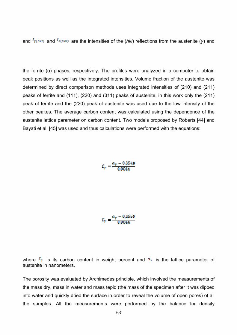
63
and and are the intensities of the (hkl) reflections from the austenite ( ) and
the ferrite (α) phases, respectively. The profiles were analyzed in a computer to obtain
peak positions as well as the integrated intensities. Volume fraction of the austenite was
determined by direct comparison methods uses integrated intensities of (210) and (211)
peaks of ferrite and (111), (220) and (311) peaks of austenite, in this work only the (211)
peak of ferrite and the (220) peak of austenite was used due to the low intensity of the
other peakes. The average carbon content was calculated using the dependence of the
austenite lattice parameter on carbon content. Two models proposed by Roberts [44] and
Bayati et al. [45] was used and thus calculations were performed with the equations:
where is its carbon content in weight percent and is the lattice parameter of austenite in nanometers.
The porosity was evaluated by Archimedes principle, which involved the measurements of
the mass dry, mass in water and mass tepid (the mass of the specimen after it was dipped
into water and quickly dried the surface in order to reveal the volume of open pores) of all
the samples. All the measurements were performed by the balance for density
64
determinations Mettler Toledo AG285 which permitted to evaluate the mean porosity with
the calculations listed below.
A = mass dry, B = mass tepid, C = mass in water
B - A = volume of open pores (cm3)
B - C = exterior volume (cm3)
100*(B - A)/(B - C) = volume of open porosity
A/(B-C) = density (g/cm3)
100-[((A/(B-C))*100)/theoretical density] = mean porosity (%)
(where the theoretical density has been chosen equal to 7,22 g/cm3)
The hardness was measured by using Vickers method, performed by Wolpert Universal
Hardness Tester, under 3 different loads (20, 30 and 40 kg) and determined as the
average value of at least 10 readings. The length of the diagonals of the pyramid indent
were measured and the average of the measurements gave back the value of hardness
listed in the manual of the hardness tester. The hardness was measured on samples
grinded and polished but un-etched.
6.4. Fracture mechanism analysis
Samples of ADI were pulled as tensile test in order to investigate the fracture mechanism.
Besides this experiment was carried out to compare the behavior when the material is
subjected to static load (present test) to dynamic load (fatigue test, introduced in the
coming paragraph). The aim of experiment is make a qualitative analysis about the
behavior of the material when a static load is applied and investigate the fracture
mechanism in ADI.
The test was performed by Scanning Electron Microscopy (SEM) to evaluate the favourite
sites where the crack nucleation occurs, which is the favourite path for the crack
propagation, and, in general, make considerations about the fracture mechanism showed
by the material. The tensile load was applied in the SEM and increased step by step in
order to analyze the entire surface of the specimen and estimate where the cracks
occurred and propagated. A preload of 25 MPa was applied and the load was increased
step by step from 25 to 1000 MPa.
The samples utilized for this purpose were extracted from the rings and machined in order
to obtain a suitable shape for the SEM (see Figure 6.5). Then they were polished and

65
etched with either Nital 3% or Picric acid 3% to elucidate the different phases in the
microstructure.
Figure 6.5: sample for fracture mechanism analysis performed by SEM.
Figure 6.6: sample mounted on the tensile device of SEM.
6.5. Impact test In order to determine the impact energy of ADI materials, the standard Charpy-type impact
test for austempered ductile iron was performed following the standard ASTM A 327M. All
the impact tests were carried out by ESAB.
All the tests were conducted at ambient conditions, using a pendulum-type impact
machine with a capacity of at least 150 Joule. The impact tests were conducted to un-
notched Charpy bars, with square cross section 10x10 mm and 55 mm of length, as

66
suggested in the standard adopted (see Figure 6.7). The samples were extracted from the
different positions (inner, middle and outer position and normal cutting direction) for each
ring and then machined in order to achieve the desirable shape and a smooth surface.
Figure 6.7: dimensions of un-notched Charpy bar impact test specimen.
The impact test was performed for all the alloys and the impact energy, or the energy
absorbed by the material during the impact, necessary to break it, calculated assuming
that its equal to one lost by the pendulum, was expressed in Joule.
Postfailure fractographic analysis was performed with Scanning Electron Microscopy
(SEM) to evaluate the fracture surface of the broken samples.
6.6. Fatigue Crack Growth Rate test Measurement of Fatigue Crack Growth Rates (FCGR) were conducted following the
standard ASTM E 647. This test method covers the determination of fatigue crack growth
rates from near-Threshold to Kmax controlled instability. The fatigue crack growth rate
(da/dN) is expressed as crack extension per cycle of loading. The stress intensity factor
range (ΔK) is the variation in stress intensity factor in a cycle, that is ΔK = Kmax - Kmin,
where Kmax is the maximum stress intensity factor or the maximum value of the stress
intensity factor in a cycle, this value corresponds to σmax, and Kmin is the minimum value of
the stress intensity factor in a cycle, this value corresponds to σmin when R>0 and is taken
to be zero when R<=0 (see Figure 6.8).
All tests were carried out in pull-push mode at room temperature in laboratory air, using a
servo-hydraulic INSTRON 8501 test machine in load control mode. The tests were carried
out at a frequency of 20 Hz, with a stress ratio R = σmin / σmax = -1 and 0. The load was
varied during the test in order to achieve the entire curve for each material, from Threshold

67
value, defined as the asymptotic value of ΔK at which da/dN approaches zero, to critical K
value, for which the crack growth rate increases to failure.
Figure 6.8: choice of Kmax ad Kmin for stress ratio R = 0, -1.
Not all the alloys were tested, only Alloy 2 and 3. It has been chosen these alloys to
compare the newest material (Alloy 3) to the oldest (Alloy 2), in order to evaluate the real
improvements and realize that both alloys fulfill the standard demands.
The samples utilized in this test measured 200 mm in length, 20 mm in width and 5 mm in
thickness (rectangular cross section 20x5 mm, see Figure 6.9). They were extracted from
the rings and then machined in order to achieve the shape predicted in the standard. The
samples were polished to facilitate the measurements of the crack length and to observe
the propagation of the crack in order to make consideration about the fracture mechanism.
In each specimen was created a notch on one of its side, approximately in the middle
position; it was made by hacksaw and then measured its length before start the test.
To measure the length of the crack the test machine was stopped and the length was
evaluated by optical microscope 50x magnification, resolution better than 0,01 mm (see
Figure 6.10).

68
Figure 6.9: dimensions of sample for fatigue crack growth rate test.
Figure 6.10: equipment utilized in the fatigue crack growth rate test.
At the end of the experiment the length of the crack (a) in relation to the number of cycles
(N) along the duration of the test has been achieved and a graphic as one shown in Figure
6.11 has plotted.

69
500000 1000000 1500000 2000000 2500000 30000000
5
10
15
20
Cra
ck le
ngth
, a [m
m]
Number of cycles, N
da1
dN1
da2
dN2
Figure 6.11: example of relation crack length-number of cycles achieved in the fatigue test.
The relation between crack length (a) and number of cycles (N) has been derived to obtain
the slope of the curve for each point (da/dN), as shown in Figure 6.11.
To achieve the stress intensity factor range was used the following formula:
where: Δσ is the stress range but, in order that R is equal to 0 and -1, Δσ = σmax;
a is the crack length;
and is a geometrical factor determined as [46]:
The results have been plotted as da/dN as a function of ΔK and log(da/dN) as a function of
log(ΔK), as commonly used (see Figure 6.12).
The slope of the linear part of curve achieved plotting log(da/dN) vs log(ΔK) was
measured (see Figure 6.12). The slope of that curve is the same parameter (called m)
which appears in the Paris law, a law that describe the behavior of the curve in the linear
part:

70
So, since da/dN and ΔK were experimentally determined, and m calculated measuring the
slope of the linear part of the curve, it has been possible to calculate the constant C.
2,2 2,4 2,6 2,8 3,0
-10
-9
-8
-7
-6
log
da/d
N
log ΔK
m
must be avoided
Figure 6.12: example of log(da/dN) vs log(ΔK), and calculation of m.
Postfailure fractographic analysis was performed with Scanning Electron Microscopy
(SEM) to evaluate the fracture surface of the broken samples.
71
7. RESULTS AND DISCUSSION
The aim of this chapter is to show the analysis results of the investigated ADI-material.
7.1. Characterization 7.1.1. Light Optical Microscope
Microstructure characterization The pictures below show the morphology changes with austempering temperature for the
investigated ADI-alloys studied.

72

73
Figure 7.1: magnification of ADI microstructure for different austempering temperatures
(respectively 360, 385 and 400 °C) for the same austenitization temperature (880°C) of
Alloy1.
Concerning the microstructure, as can observed in Figure 7.1, the brown needles
represent the ausferrite (or acicular ferrite). They are interconnected by lighter areas,
which correspond to retained austenite. The dark gray dots features are the graphite
nodules.
Looking at the pictures above a clear difference between the different austempering
temperatures is hard to see. That might be explained by the slightly different of the
austempering temperatures chosen.
However, more small regions of retained austenite and an increase of the thickness of
ausferrite needles could be seen when the austempering temperature increases from 360
°C to 400 °C. Therefore a qualitative analysis of the ferrite needles was conducted. This
included the ratio between the thickness and the length of some needles of ausferrite was
measured for the samples austempered at different temperatures (see Figure 7.2). At least
5 measurements for each specimen were performed, and the increase of the ratio aspect
increasing the austempering temperature was confirmed (Figure 7.3).This result is in
agreement with the literature [5] which asserts that at low austempering temperatures, due
to high cooling, a high nucleation rate results in a large number of fine ferrite needles and,
on the other hand, at higher temperatures, the lower nucleation rate results in fewer ferrite
needles, each growing to a larger size. In fact, increasing the austempering temperature,
resulted in the coarsening of the bainitic ferrite as well as an increase in the austenite
content, as described in the previous paragraphs.

74
Figure 7.2: example of measurement of thickness and ratio of ausferrite needles.
350 360 370 380 390 400 4100,00
0,02
0,04
0,06
0,08
0,10
0,12
Aspe
ct ra
tio o
f aus
ferri
te n
eedl
es
Austempering temperature [°C] Figure 7.3: relation between aspect ratio of ausferrite needles and austempering
temperature for ADIs studied.
The pictures below show the variation on the microstructure for the austenitization
temperatures for Alloy 1(840, 860 and 880 °C, see Figure 7.4).
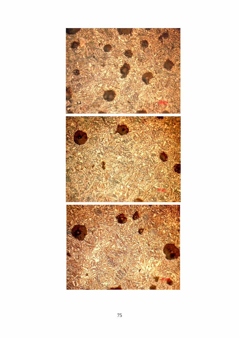
75
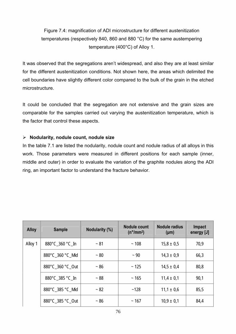
76
Figure 7.4: magnification of ADI microstructure for different austenitization
temperatures (respectively 840, 860 and 880 °C) for the same austempering
temperature (400°C) of Alloy 1.
It was observed that the segregations aren’t widespread, and also they are at least similar
for the different austenitization conditions. Not shown here, the areas which delimited the
cell boundaries have slightly different color compared to the bulk of the grain in the etched
microstructure.
It could be concluded that the segregation are not extensive and the grain sizes are
comparable for the samples carried out varying the austenitization temperature, which is
the factor that control these aspects.
Nodularity, nodule count, nodule size In the table 7.1 are listed the nodularity, nodule count and nodule radius of all alloys in this
work. Those parameters were measured in different positions for each sample (inner,
middle and outer) in order to evaluate the variation of the graphite nodules along the ADI
ring, an important factor to understand the fracture behavior.
Alloy Sample Nodularity (%) Nodule count (n°/mm2)
Nodule radius (μm)
Impact energy [J]
880°C_360 °C_In ~ 81 ~ 108 15,8 ± 0,5 70,9
880°C_360 °C_Mid ~ 80 ~ 90 14,3 ± 0,9 66,3
880°C_360 °C_Out ~ 86 ~ 125 14,5 ± 0,4 80,8
880°C_385 °C_In ~ 88 ~ 165 11,4 ± 0,1 90,1
880°C_385 °C_Mid ~ 82 ~128 11,1 ± 0,6 85,5
Alloy 1
880°C_385 °C_Out ~ 86 ~ 167 10,9 ± 0,1 84,4

77
880°C_400 °C_In ~ 85 ~ 179 10,9 ± 0,7 94,6
880°C_400 °C_Mid ~ 82 ~ 140 10,4 ± 0,1 104,2
880°C_400 °C_Out ~ 84 ~ 178 11,0 ± 0,6 112,4
840°C_400 °C_In ~ 86 ~ 242 7,5 ± 0,1 112,0
840°C_400 °C_Mid ~ 79 ~ 53 7,9 ± 0,2 108,1
840°C_400 °C_Out ~ 82 ~ 186 6,9 ± 0,2 113,6
860°C_400 °C_In ~ 83 ~ 170 7,7 ± 0,1 121,0
860°C_400 °C_Mid ~ 79 ~ 59 8,1 ± 0,3 93,5
860°C_400 °C_Out ~ 85 ~ 169 7,3 ± 0,1 97,3
840°C_400 °C_In ~ 82 ~ 86 7,5 ± 0,2 97,8
840°C_400 °C_Mid ~ 73 ~ 41 7,2 ± 0,1 60,7 Alloy 2
840°C_400 °C_Out ~ 83 ~ 66 7,4 ± 0,6 106,1
840°C_400 °C_In ~ 85 ~ 114 6,7 ± 0,3 113,6
840°C_400 °C_Mid ~ 80 ~ 59 7,3 ± 0,4 84,8
Alloy 3 840°C_400 °C_Out ~ 85 ~ 96 7,0 ± 0,2 106,5
Table 7.1: nodularity, nodule count,nodule radius and impact energy for the ADIs studied.
As shown in table 7.1, the nodularity is higher than 80% for almost all the specimens. This
is an important factor because the graphite nodule has a “micronotch” effect on the
microstructure and can strongly affect the properties [13]. Higher nodularity means more
graphite nodules of spheroidal shape and lower stress concentration factors as compared
to other nonspheroidal shapes [13]. In addition, spheroidal nodules have less sites for the
protrusion of graphite into matrix. This develops a less stress concentration at
graphite/matrix interface.
The size of the nodules in the different samples is quite variable and can be noticed that
for Alloy 1, for which the heat treatment was investigated, the sample with the biggest
nodule size shows the smallest nodule count, and decreasing the nodule radius could be

78
seen an increase of nodule count, however when the nodule size becomes slightly
different there isn’t a relation between nodule count and nodule size.
Furthermore it can be noticed that, inside each kind of material (same alloy different heat
treatment conditions as well), the nodularity and the nodule count in the middle part of the
ring are lower than inner and middle parts. This might be due to the fact that inner part of
the rings is the last one to solidify.
Finally, it can be seen that, for the three different alloys (different chemical composition)
but same heat treatment conditions, the nodularity and nodule size are comparable, while
the nodule count is higher for Alloy 1.
7.1.2. X-Ray analysis By X-Ray Diffraction it was evaluated the amount of retained austenite (Xγ) and its carbon
content (Cγ). The results are listed in the table 7.2.
There are two values of carbon content of retained austenite because it was measured
according to two different references (respectively Roberts and Bayati). The carbon
content predicted by Roberts is higher but, however, the different samples keep the same
rank in the two calculation.
Alloy Sample Retained Austenite, Xγ (%) Carbon content, Cγ (%) Roberts Bayati
880°C_360 °C 29,6 1,87 1,72
880°C_385 °C 24,5 1,85 1,69
880°C_400 °C 22,6 1,86 1,71
860°C_400 °C 26,0 1,84 1,68
Alloy 1
840°C_400 °C 20,9 1,90 1,74
Alloy 2 840°C_400 °C 32,5 1,90 1,74
Alloy 3 840°C_400 °C 34,6 1,82 1,66
Table 7.2: amount of retained austenite and its carbon content for the ADIs studied.

79
The first observation is that the carbon content range is slightly different for Alloy 1
(maximum value is 1,90 and the minimum is 1,82 for Roberts, 1,74 and 1,66 for Bayati). It
might be due to the small difference between the austenitization temperature, which
controls the carbon content of the matrix.
The amount of retained austenite increases when the austempering temperature
decreases, for the samples austenitized at the same temperature (880 °C, Alloy 1). This is
not in agreement with what asserted by the literature.
In the samples austempered at the same temperature (400 °C), it can’t be noticed a
relation with the variation of austenitization temperature, which controls the carbon content
of retained austenite. In fact the value of carbon reaches the maximum at 840 °C.
Comparing the three alloys with different chemical composition but same austenitization
and austempering temperatures, Alloy 1 shows the lowest amount of retained austenite
but the highest percentage of carbon content, which leads to the stability of retained
austenite. But the amount of retained austenite is noticeably higher in Alloy 2 and 3. The
difference might be due to the different austenitization times (75 minutes for Alloy 1, 90
minutes for Alloy 2 and 3).
7.1.3. Porosity The measure of porosity listed in table 7.3 shows that it’s comparable for all the specimens
studied. In fact the values of the mean porosity are slightly different for all the samples.
The mean porosity is less than 1% for all the alloys, that means porosity is not, at least,
the most important defect for the materials studied; the most dangerous defects are dross
shrinkages, than porosities.
Alloy Sample Mean Porosity
880°C_360 °C_In 0,17
880°C_360 °C_Out 0,08 0,13 ± 0,07
Alloy 1
880°C_385 °C_In 0,27 0,28 ± 0,03

80
880°C_385 °C_Out 0,30
880°C_400 °C_In 0,88
880°C_400 °C_Out 0,78 0,83 ± 0,07
840°C_400 °C_In 0,63
840°C_400 °C_Out 0,95 0,79 ± 0,22
860°C_400 °C_In 0,69
860°C_400 °C_Out 0,69 0,69 ± 0,00
840°C_400 °C_In 0,32 Alloy 2
840°C_400 °C_Out 0,20 0,26 ± 0,09
840°C_400 °C_In 0,11 Alloy 3
840°C_400 °C_Out 0,41
0,26 ± 0,21
Table 7.3: porosity determined for ADI samples studied.
7.1.4. Hardness In the table below are listed the values of hardness (Vickers) measured for the different
alloys studied.
Alloy Sample Vickers Hardness (HV)
880°C_360 °C_In 351,6 ± 4,9
880°C_360 °C_Out 380,8 ± 10,2 366,2 ± 16,9
880°C_385 °C_In 355,2 ± 29,7
880°C_385 °C_Out 326,8 ± 10,1 341,0 ± 25,4
Alloy 1
880°C_400 °C_In 314,7 ± 15,3 308,0 ± 14,3

81
880°C_400 °C_Out 301,2 ± 9,2
840°C_400 °C_In 291,6 ± 5,0
840°C_400 °C_Out 304,4 ± 9,5 298,0 ± 9,9
860°C_400 °C_In 295,5 ± 7,7
860°C_400 °C_Out 333,3 ± 17,4 314,4 ± 23,4
840°C_400 °C_In 284,6 ±12,1 Alloy 2
840°C_400 °C_Out 285,6 ± 6,5 285,1 ± 5,8
840°C_400 °C_In 265,5 ± 5,8 Alloy 3
840°C_400 °C_Out 268,6 ± 7,1 267,1 ± 7,1
Table 7.4: values of hardness for ADIs tested.
In Alloy 1, for which different austenitization and austempering conditions were studied,
the hardness shows an increase when the austempering temperature decreases. This is in
agreement with the literature data , which shows an enhance of strength (with a optimum
combination of ultimate tensile strength, yield strength and hardness) when the
austempering temperature decreases. Anyway the variation between the different
austempering temperatures is small, so the hardness values are comparable into the
same range considering the standard deviation.
The variation of austenitization temperature doesn’t show the same effect.
In the alloy with different chemical composition but same austenitization and austempering
conditions the values of hardness are slightly different, and it’s not possible to predict a
relation between them.
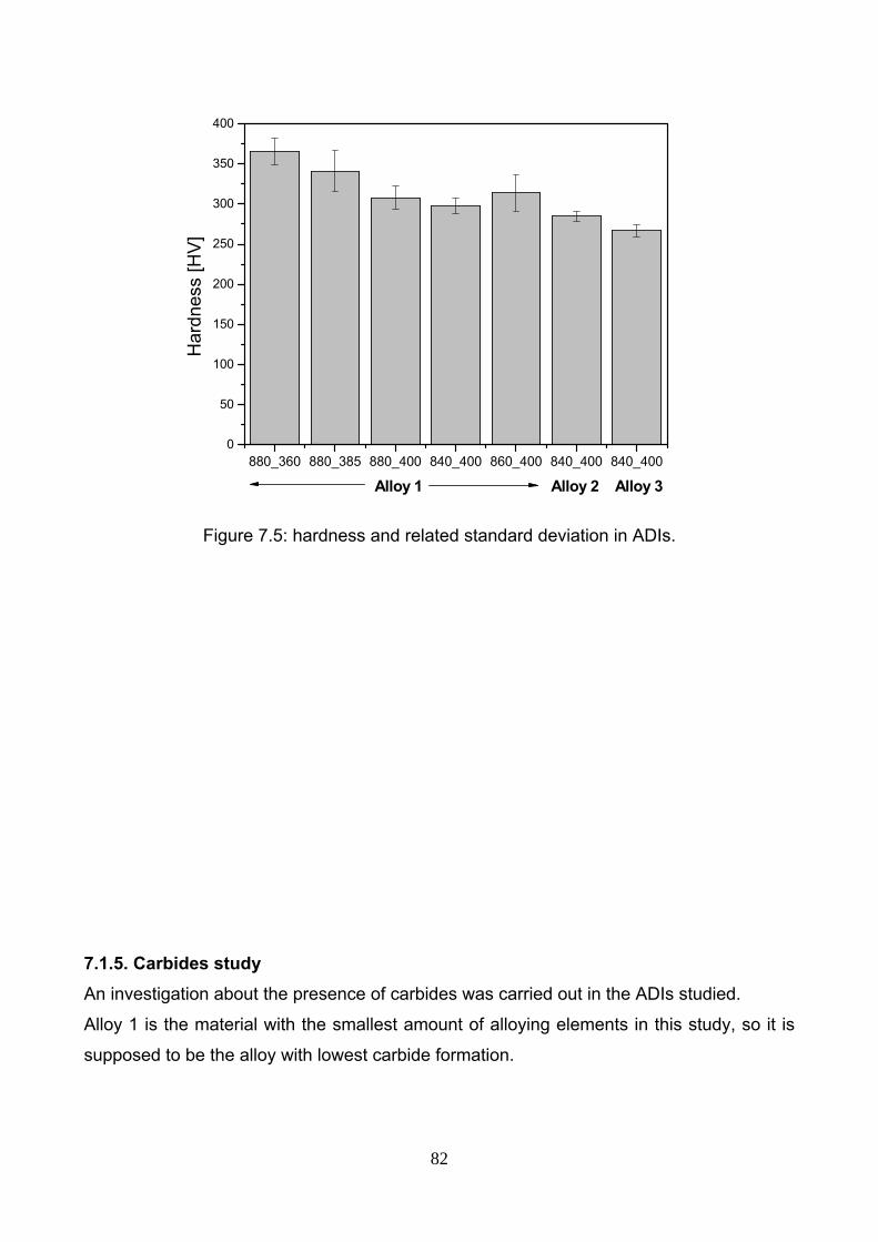
82
880_360 880_385 880_400 840_400 860_400 840_400 840_4000
50
100
150
200
250
300
350
400
Har
dnes
s [H
V]
Alloy 1 Alloy 2 Alloy 3
Figure 7.5: hardness and related standard deviation in ADIs.
7.1.5. Carbides study An investigation about the presence of carbides was carried out in the ADIs studied.
Alloy 1 is the material with the smallest amount of alloying elements in this study, so it is
supposed to be the alloy with lowest carbide formation.

83
Figure 7.6: carbides in Alloy 1 for different austempering temperature.
From Figure 7.6, a slightly increase of amount of carbides can be observed when the
austempering temperature decreases from 360 to 400 °C in Alloy 1. However, since the
percentage of carbides is very low, it wasn’t possible to quantify the amount of carbides for
the different heat treatment conditions in Alloy 1.
In all the cases, the carbides formation occurs in the cell boundary, where the alloying
element segregate during the solidification of the material.
On the other hand, Alloy 2 is the material with highest percentage of alloy elements,
compared to Alloy 1 and 3. It means that a larger amount of carbides should be expected.

84
Figure 7.7: etched and heat tinted microstructure of Alloy 2.
The microstructure in Figure 7.7 shows the presence of the cell boundary segregation in
Alloy 2. It can be seen also the formation of carbides at the cell boundary, they are present
as white spots or for flattened shape, as it can be noticed on the heat tinted microstructure
on the right.
Figure 7.8: heat tinted microstructure of Alloy 2.
Figure 7.8 shows the presence of carbides in higher magnification. It is also possible to
see bright areas that could be indentified as martensite or low carbon austenite. It’s very
hard, also for an expert eye, to distinguish which phase it is, but, if it is low carbon
austenite, it may transform to martensite when a load is applied, due to its instability
caused by its low carbon concentration.

85
Figure 7.9: some defects in Alloy 2 microstructure revealed by SEM.
As shown in Figure 7.9, the carbide (white) is surrounded by porosity, which may be a
crack initiation site. Also in Figure 7.9 a small area that could be martensite could also be
seen.
Figure 7.10: carbide in Alloy 2 revealed by SEM.
Also in Figure 7.10 it can be noticed porosity along the boundary of the carbide. Besides
the EDS analysis carried out for some carbides detected in the microstructure, has

86
revealed the presence of Molybdenum as main element as well as traces of Titanium and
Vanadium (Figure 7.11).
Figure 7.11: EDS analysis of the carbide showed on figure 5.
Alloy 3 has also a small amount of carbides, which is expected of the alloying elements in
this alloy are less than in Alloy 2, but slightly higher than in Alloy 1.
Figure 7.12: carbide in Alloy 3 revealed by SEM.
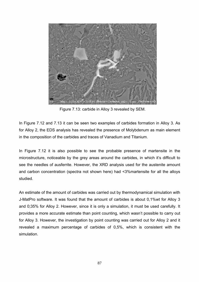
87
Figure 7.13: carbide in Alloy 3 revealed by SEM.
In Figure 7.12 and 7.13 it can be seen two examples of carbides formation in Alloy 3. As
for Alloy 2, the EDS analysis has revealed the presence of Molybdenum as main element
in the composition of the carbides and traces of Vanadium and Titanium.
In Figure 7.12 it is also possible to see the probable presence of martensite in the
microstructure, noticeable by the grey areas around the carbides, in which it’s difficult to
see the needles of ausferrite. However, the XRD analysis used for the austenite amount
and carbon concentration (spectra not shown here) had <3%martensite for all the alloys
studied.
An estimate of the amount of carbides was carried out by thermodynamical simulation with
J-MatPro software. It was found that the amount of carbides is about 0,1%wt for Alloy 3
and 0;35% for Alloy 2. However, since it is only a simulation, it must be used carefully. It
provides a more accurate estimate than point counting, which wasn’t possible to carry out
for Alloy 3. However, the investigation by point counting was carried out for Alloy 2 and it
revealed a maximum percentage of carbides of 0,5%, which is consistent with the
simulation.

88
7.2. Impact test The impact energies for all the ADIs materials studied are showed in the following
graphics (Figures 7.14 and 7.15).
Figure 7.14: impact energies of all the materials shared by sample location on ring,
maximum and minimum values are indicated.
In Figure 7.14 it can be seen a big scattering around the average values for many
samples. However it can be noticed, in general, lower impact energy for the samples
located in the middle of the ring. This is due to the “microstructure quality” of the material
in that location. In fact, the middle part of the ring is the last one to solidify so the
segregation of alloy elements is higher than the inner and outer part of the ring, so
probably the concentration of carbides and defects is more elevated. The presence of
defects lead to decrease the impact properties of ADI, and probably it is also the cause of
the big scattering shown by the impact energies.
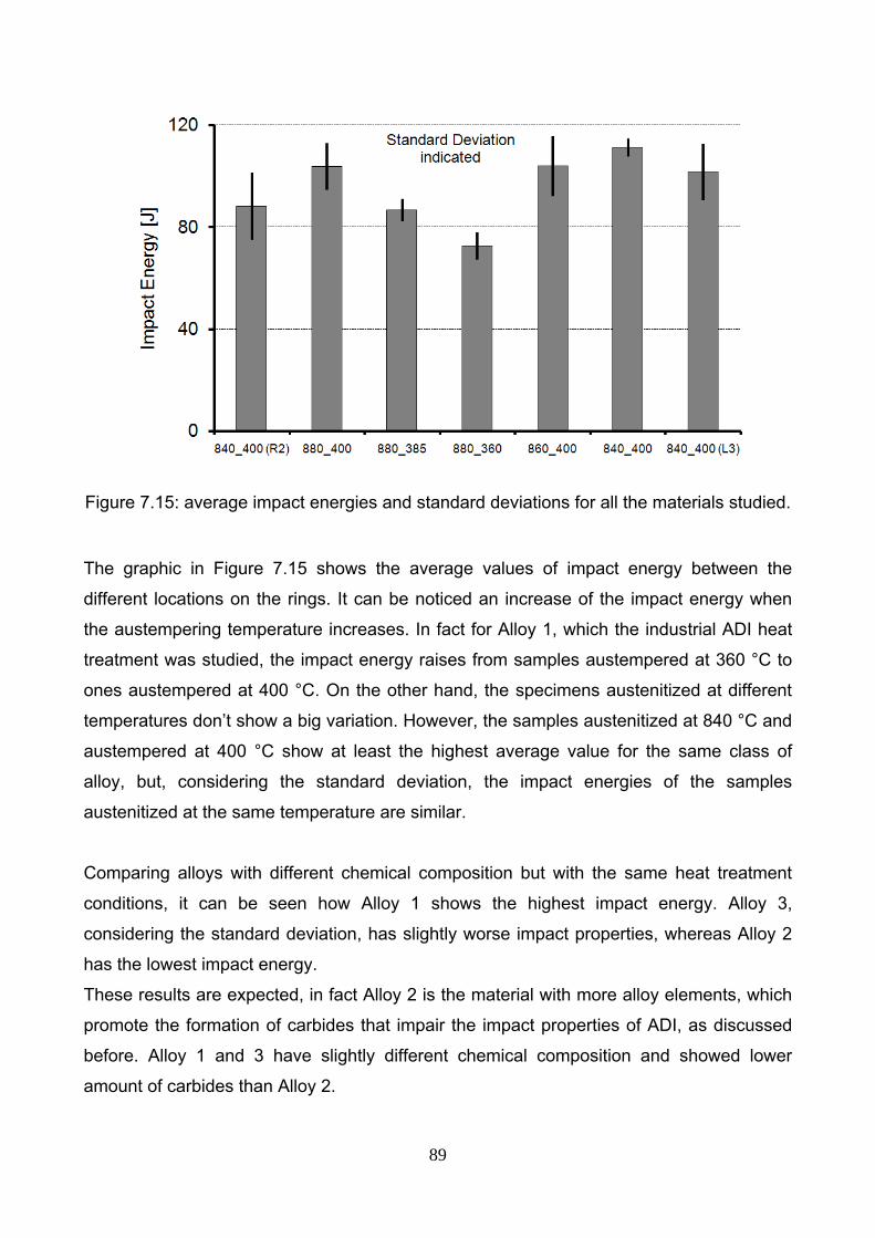
89
Figure 7.15: average impact energies and standard deviations for all the materials studied.
The graphic in Figure 7.15 shows the average values of impact energy between the
different locations on the rings. It can be noticed an increase of the impact energy when
the austempering temperature increases. In fact for Alloy 1, which the industrial ADI heat
treatment was studied, the impact energy raises from samples austempered at 360 °C to
ones austempered at 400 °C. On the other hand, the specimens austenitized at different
temperatures don’t show a big variation. However, the samples austenitized at 840 °C and
austempered at 400 °C show at least the highest average value for the same class of
alloy, but, considering the standard deviation, the impact energies of the samples
austenitized at the same temperature are similar.
Comparing alloys with different chemical composition but with the same heat treatment
conditions, it can be seen how Alloy 1 shows the highest impact energy. Alloy 3,
considering the standard deviation, has slightly worse impact properties, whereas Alloy 2
has the lowest impact energy.
These results are expected, in fact Alloy 2 is the material with more alloy elements, which
promote the formation of carbides that impair the impact properties of ADI, as discussed
before. Alloy 1 and 3 have slightly different chemical composition and showed lower
amount of carbides than Alloy 2.

90
Effect of the graphite nodules
70 75 80 85 90 950
20
40
60
80
100
120
Impa
ct e
nerg
y [J
]
Nodularity (%)
Alloy1 840_400
Alloy1 880_400Alloy1 860_400
Alloy2 840_400 Alloy1 880_385
Alloy3 840_400
Alloy1 880_360
Figure 7.16: relation between impact energy and nodularity for ADIs studied.
As shown in Figure 7.16, the nodularity affects the impact energy, in fact increasing the
nodularity, the “notch effect” inside the material is lower and the impact energy increases.
However, the values of nodularity of the materials studied are comprised in a small range,
so it can’t be seen a clear relation between nodularity and impact properties.
However, it was observed that the nodularity doesn’t depend on the heat treatment,
neither of the composition. The main factor is the cooling rate during the casting. It can be
observed in Figure 7.17, the variation of nodularity in the ring location for Alloy 1, for which
the ADI heat treatment was studied: the middle part of the ring is the one which the cooling
is more slowly and the values of nodularity are lower, independently of the heat treatment.
In fact there is no relation between nodularity and heat treatment conditions, but in each
sample, the nodularity shows the lowest value in the middle part of the ring.

91
880_360 880_385 880_400 860_400 840_400
79
80
81
82
83
84
85
86
87
88
89
inner position middle position outer position
Nod
ular
ity (%
)
Figure 7.17: variation of nodularity in the ring location in Alloy 1.
0 50 100 150 200 2500
20
40
60
80
100
120 Alloy1 840_400
Alloy1 880_400
Alloy1 860_400
Alloy2 840_400 Alloy1 880_385
Alloy3 840_400
Impa
ct e
nerg
y [J
]
Nodule count [n°/mm2]
Alloy1 880_360
Figure 7.18: relation between impact energy and nodule count for ADIs studied.

92
It can be noticed in Figure 7.18 that the impact energy increases when the nodule count
increases. The way to optimize the number of nodules is determined by the composition
and the casting before the heat treatment.
As shown in the previous paragraph, the alloy that shows the highest number of graphite
nodules is Alloy 1, which it’s also the material that shows higher impact properties.
Alloy 1 Alloy 2 Alloy 30
20
40
60
80
100
120
140
160
180
200
220
240
260
280
Nod
ule
coun
t [n°
/mm
2 ]
Figure 7.19: nodule count in the different alloys for the same heat treatment conditions.
The alloy element that promotes the formation of nodules of graphite is the silicon. The
silicon promotes graphite formation, decreases the solubility of carbon in austenite,
increases the eutectoid temperature and inhibits the formation of bainitic carbides [1]. The
most important factor to achieve high nodule count is to be near to the eutectoid point, in
order to increase the inoculation [1].
Moreover has been observed that the austenitization temperature or the austempering
temperature do not affect to the number of nodules. It could be concluded that, in order to
obtain good impact properties, a composition that promotes the formation of graphite
nodules must be selected, due to the subsequent heat treatment will not change this
parameter.

93
6 8 10 12 14 160
20
40
60
80
100
120
Impa
ct e
nerg
y [J
]
Nodule radius [μm]
Alloy1 840_400Alloy1 880_400
Alloy1 860_400
Alloy2 840_400
Alloy1 880_385
Alloy3 840_400
Alloy1 880_360
Figure 7.20: relation between impact energy and nodule radius for ADIs studied.
As shown in Figure 7.20, another important factor for the impact properties is the size of
the graphite nodules. The results show an increase of impact energy when the size of the
graphite nodules decreases.
Moreover, it can be observed that the austenitization temperature is connected with the
size of the nodules. As shown in Figure 7.21, increasing the austenitization temperature,
the nodule size increases, for the sample austempered at the same temperature in Alloy 1.
This result is not expected. In fact, the austenitization temperature should slightly affect
the nodule size [1], and, moreover, in the opposite way [1]. So, probably, the growth of
nodule radius when the austenitization temperature increases, is only a particular case of
the samples studied.
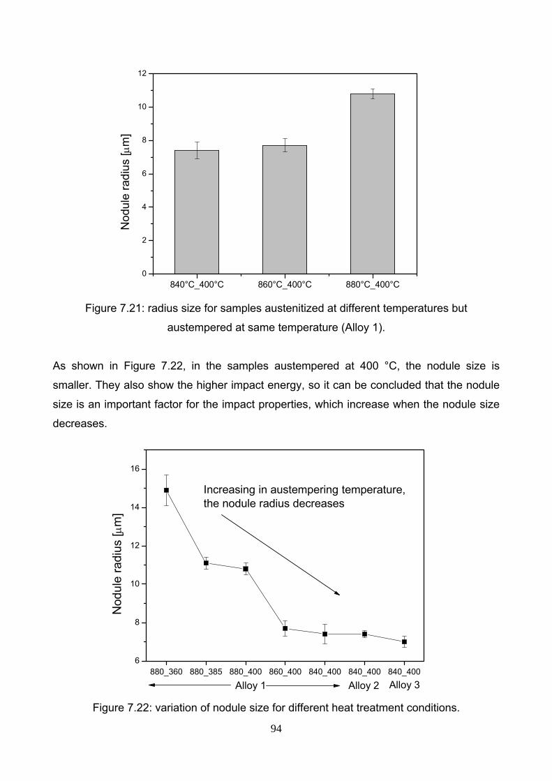
94
840°C_400°C 860°C_400°C 880°C_400°C0
2
4
6
8
10
12
Nod
ule
radi
us [μ
m]
Figure 7.21: radius size for samples austenitized at different temperatures but
austempered at same temperature (Alloy 1).
As shown in Figure 7.22, in the samples austempered at 400 °C, the nodule size is
smaller. They also show the higher impact energy, so it can be concluded that the nodule
size is an important factor for the impact properties, which increase when the nodule size
decreases.
880_360 880_385 880_400 860_400 840_400 840_400 840_4006
8
10
12
14
16
Nod
ule
radi
us [μ
m]
Increasing in austempering temperature, the nodule radius decreases
Alloy 1 Alloy 2 Alloy 3 Figure 7.22: variation of nodule size for different heat treatment conditions.

95
Effect of retained austenite
20 22 24 26 28 30 32 34 360
20
40
60
80
100
120Alloy 3 840_400
Alloy 2 840_400
Alloy 1 840_400
Alloy 1 860_400
Alloy 1 880_400Alloy 1 880_385
Impa
ct e
nerg
y [J
]
Retained Austenite (%)
Alloy 1 880_360
Figure 7.23: relation between impact energy and amount of retained austenite for ADIs
studied.
The amount of retained austenite is another important factor, in particular for the fracture
toughness of ADI, as explained in the literature review.
In this study, as shown in Figure 7.23, there is not a clear relation between impact
properties and amount of retained austenite. In fact, for instance, the sample with the
lowest amount of retained austenite (Alloy 1 austenitized at 840 °C and austempered at
400 °C) is the one which has the highest impact energy (at least considering the average
value). However, Alloy 3 shows the highest amount of retained austenite as well as
elevated impact energy.
It could be concluded that, probably the effect of the graphite nodules affects more than
the amount of retained austenite, in the ADIs studied.

96
Fractographic analysis
An investigation of the surface of the failed samples after the impact test was carried out
by Scanning Electron Microscope (SEM). It was analyzed the fracture surface of the
samples which showed higher and lower impact energies.
Figure 7.24: comparison between sample with higher and lower impact energy
respectively.
It can be noticed in Figure 7.24 that the sample with lower impact energy (on the right),
shows graphite nodules aligned in a row (pointed out by the blue ovals in the picture). That
doesn’t appear in the fracture surface of the sample with higher energy. In Figure 7.25 it
can be observed tha the cleaved surfaces are fingerprinted by the ausferrite structure,
which means that the fingerprint for Alloy 1 austempered at 400°C was wider and deeper.
In Figures 7.26 and 7.27 evidence of graphite nodules debonding form the matrix can be
seen after the impact tests, which evidently was also the dominant mode of fracture in the
FCGR experiments. Furthermore, in Figure 7.28 the crack propagation at the cell/grain
boundary is seen. From these diagrams, it can be concluded that the crack path
preferentially intersects graphite nodules, and if the distance between the nodules are
small and the nodules aligned, the crack will propagate easily and the impact energy will
be low.
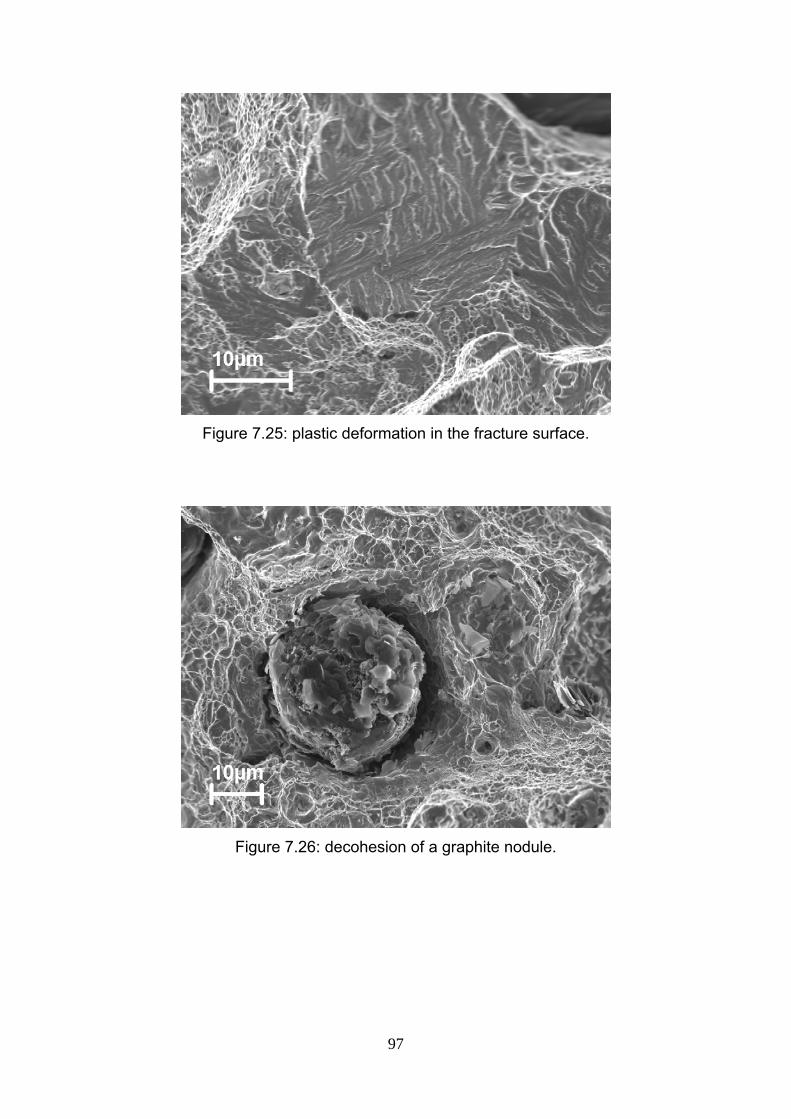
97
Figure 7.25: plastic deformation in the fracture surface.
Figure 7.26: decohesion of a graphite nodule.

98
Figure 7.27: the debonding of the graphite nodules.
Figure 7.28: crack propagation in the cell/grain boundary.

99
7.3. Fracture mechanism analysis The fracture mechanism of ADI was investigated performing a tensile test on the Scanning
Electron Microscope (SEM). The behavior of the material when the load increase was
study, analyzing the sites of nucleation of the crack and its propagation.
The behavior of the material is shown in Figure 7.29.
Figure 7.29: crack behavior in the load-deformation diagram.
It was observed that the nucleation of the cracks occurs on the defects of the material, as
pores or carbides mainly, but also due to the decohesion at the interface between matrix
and graphite nodules.
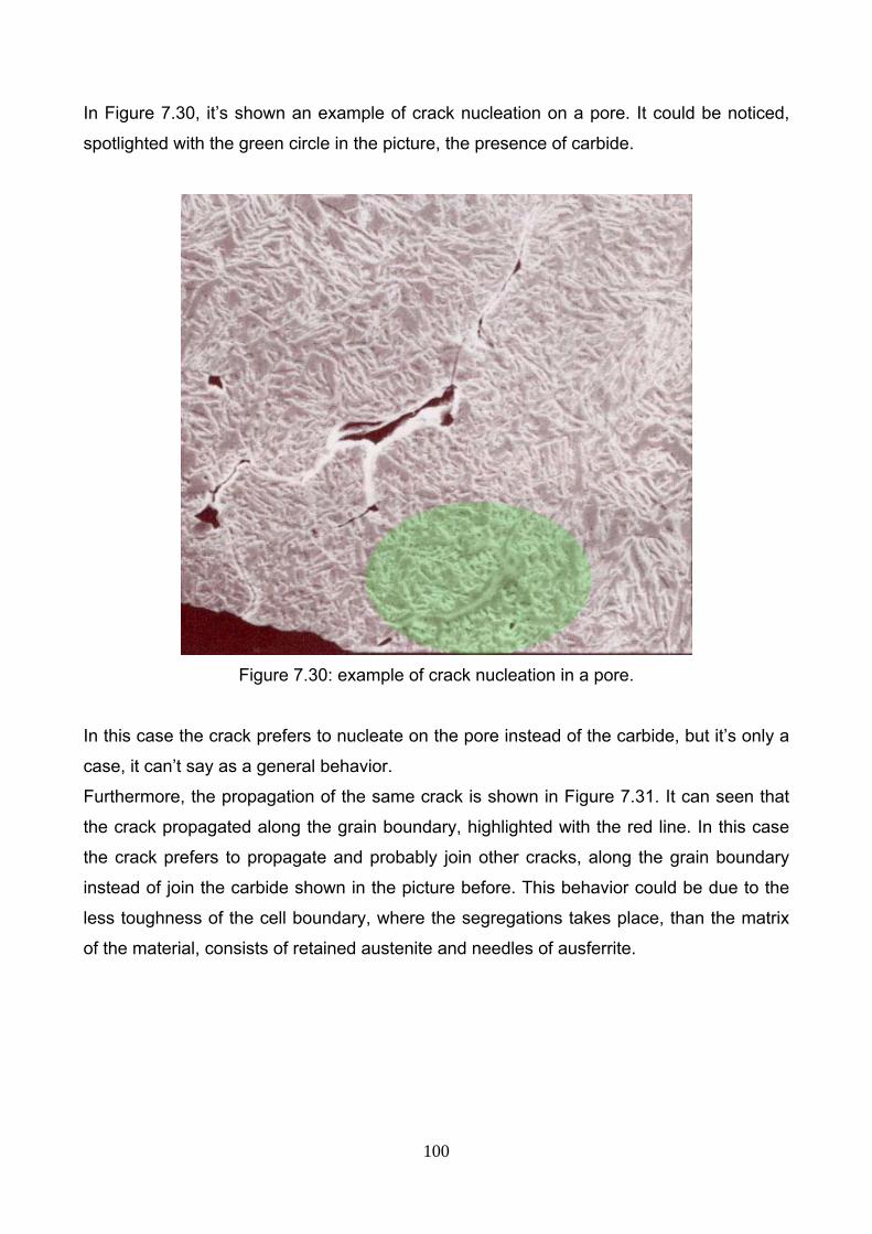
100
In Figure 7.30, it’s shown an example of crack nucleation on a pore. It could be noticed,
spotlighted with the green circle in the picture, the presence of carbide.
Figure 7.30: example of crack nucleation in a pore.
In this case the crack prefers to nucleate on the pore instead of the carbide, but it’s only a
case, it can’t say as a general behavior.
Furthermore, the propagation of the same crack is shown in Figure 7.31. It can seen that
the crack propagated along the grain boundary, highlighted with the red line. In this case
the crack prefers to propagate and probably join other cracks, along the grain boundary
instead of join the carbide shown in the picture before. This behavior could be due to the
less toughness of the cell boundary, where the segregations takes place, than the matrix
of the material, consists of retained austenite and needles of ausferrite.

101
Figure 7.31: example of crack propagation.
On the other hand, in the literature [17] it is asserted that carbides are the main
responsible of crack initiation. In this study it was found that cracks could be occur caused
by different kind of defects, but the porosity was discovered to be the most dangerous
crack initiator.

102
Another site of crack nucleation is the matrix/graphite nodule interface. In Figure 7.32 is
shown the decohesion that occurs, in Figure 7.33 a crack is propagating from a nodule.
Figure 7.32: decohesion of the graphite nodule.
It can be noticed that a large nodule size leads the formation of voids due to the
decohesion of graphite nodules as well as induced stress concentration fields. More
deformation would take place in the area near the graphite nodules which promote the
formation of cracks extending from the nodules. So it can be concluded that the crack
initiation should be easier as larger is the nodule size.

103
Figure 7.33: crack propagation from the graphite nodule/matrix interface.
It can be affirmed that the preferential crack path is between two neighboring nodules, and
the crack growth would be faster as closer are the two nodules. However, the growth can
take place along the austenite/ferrite interface or cut the ferrite laths. It’s very hard to
assert which is the easiest path for the crack growth because it was found that it depends
on the orientation of the ferrite laths. If they are oriented perpendicularly with the direction
which the load is applied, the ferrite laths might be the favourite path. On the other hand,
in this work, a preliminary XRD investigation was carried out on failed samples of ADI, and
it revealed a big amount of ferrite on the fracture surface. This supports the theory for what
the crack growth occurs along interface austenite/ferrite, but this should be investigated
further.
7.4. Fatigue Crack Growth Rate test The Fatigue Crack Growth Test allow to measure the variation of crack length (a) in
relation to the number of cycles passed during the test, as described in the experimental
procedure chapter. By that curve it was possible to evaluate the fatigue crack growth rate
(da/dN), expressed as crack extension per cycle of loading, and the stress intensity factor
range (ΔK) is the variation in stress intensity factor in a cycle: the results achieved are
shown in the following paragraph.
The graphic in Figure 7.34 shows the comparison of the fatigue crack growth behavior of
Alloy 2 and Alloy 3 for the load case R = -1.

104
1 10 10010-11
10-10
10-9
10-8
10-7
10-6
Alloy 3Alloy 2
da/d
N [m
/cyc
le]
ΔK [MPa m1/2]
R = -1
Figure 7.34: comparison of fatigue crack growth behavior of Alloy 2 and 3 for R = -1.
As shown in Figure 7.34, it can be noticed a “double branch” near the threshold in Alloy 2
when two specimens are tested. Microstructural evaluation reveals that there is a
difference in pearlite content between the two specimens. In the right specimen in Figure
7.34 there is about 25% pearlite while in the specimen to the left on average 10%
(estimation by point counting). Pearlite should not be present in ADI and this is probably
due to some error in the casting process.
In specimen 2 (left curve in Figure 7.34) the pearlite distribution is uneven, there is more
pearlite on one side. Another difference is the distribution of graphite, in both specimens
there is a skeleton of coarse graphite and a finer distribution within the area defined by the
coercer graphite. A striking difference is that coarse pearlite stringers appear in
conjunction with a band of graphite. There are also areas of local porosities in the left
specimen (specimen 1). In specimen 2 the fraction of isolated porosities is about 0,6%.

105
Figure 7:35: Example of pearlite in specimen 2, etched in Picral.
In all other microstructural parameters there are minor differences. Nodularity is between
86 and 93%, nodule count between 153 and 163 nodules/mm2. Graphite area fraction is
practically the same. To conclude, specimen 2 (left curve in Figure 7.34) seems to best
represent the properties of a pearlitic free Alloy 2–specimen. Specimen 4 (R = 0) show no
sign of pearlite. Reasons for the pearlite appearance is found both in the foundry process
(micro segregation and graphite distribution) but also in the heat treatment procedure,
possibly to long transfer time between the austenitiation furnace and the salt bath.
Alloy 3 shows a big scattering, particularly in the linear region. That’s might be explained
by the method chosen to measure the crack propagation rate. Here the local propagaton
rate on one of the outer surfaces is measured. According to the standard a smoothing
operation should be done which gives a mean value for the propagation rate over the
whole cross section. Such a procedure will eliminate most of the scatter but also hide
some of the variations caused by the local microstructure.
The slope of the linear region for the different alloys is slightly different. Value of m
(constant in the Paris region stating the slope) differs between the two specimens. The
specimen with low pearlite content has a m = 3,16 (left curve) and m = 5,15 for the right
curve (this specimen have a high pearlitic content, about 25% of the matrix). Alloy 3 has a
m value equal to 3,34. Reasons for the difference lie in the pearlite content. In the right
curve the pearlite is concentrated to bands of coerce graphite. This is probably due to
micro segregation of some chemical elements during solidification of the alloy. It´s

106
believed that the specimen with the lower pearlite content represents the “true” crack
propagation curve for Alloy 2.
The threshold value (ΔKth), equal to the stress intensity range (ΔK) for which the fatigue
crack growth rate (da/dN) reaches the minimum value, is 7,20 MPa√m for Alloy 2 and
equal to 10,35 MPa√m for Alloy 3. 10,35 MPa√m have a closer resemblance to normal
ferritc/pearlitc cast iron.
The graphic in Figure 7.36 shows the comparison of the fatigue crack growth behavior
between Alloy 2 and 3 for R = 0.
1 10 100
10-10
10-9
10-8
10-7
10-6
10-5
Alloy 3Alloy 2
da/d
N [m
/cyc
le]
ΔK [MPa m1/2]
R = 0
Figure 7.36: comparison of fatigue crack growth behavior of Alloy 2 and 3 for R = 0.
As shown in Figure 7.36, it’s a huge difference between case R = 0 for Alloy 2 and Alloy 3.
The m value for Alloy 2 is 3,14, while for Alloy 3 is 4,54. It means that the slope of the
Alloy 3 curve is higher than Alloy 2, so the fatigue crack growth rate is higher for Alloy 3
when the crack growth is linear. A striking difference is the nodule count between the two
alloys. Alloy 3 has 231 nodules/mm2 while Alloy 2 has 153 nodules/mm2. All other
parameters are quite the same. As only one specimen is tested for Alloy 3 more
investigations must be implemented for this load case.
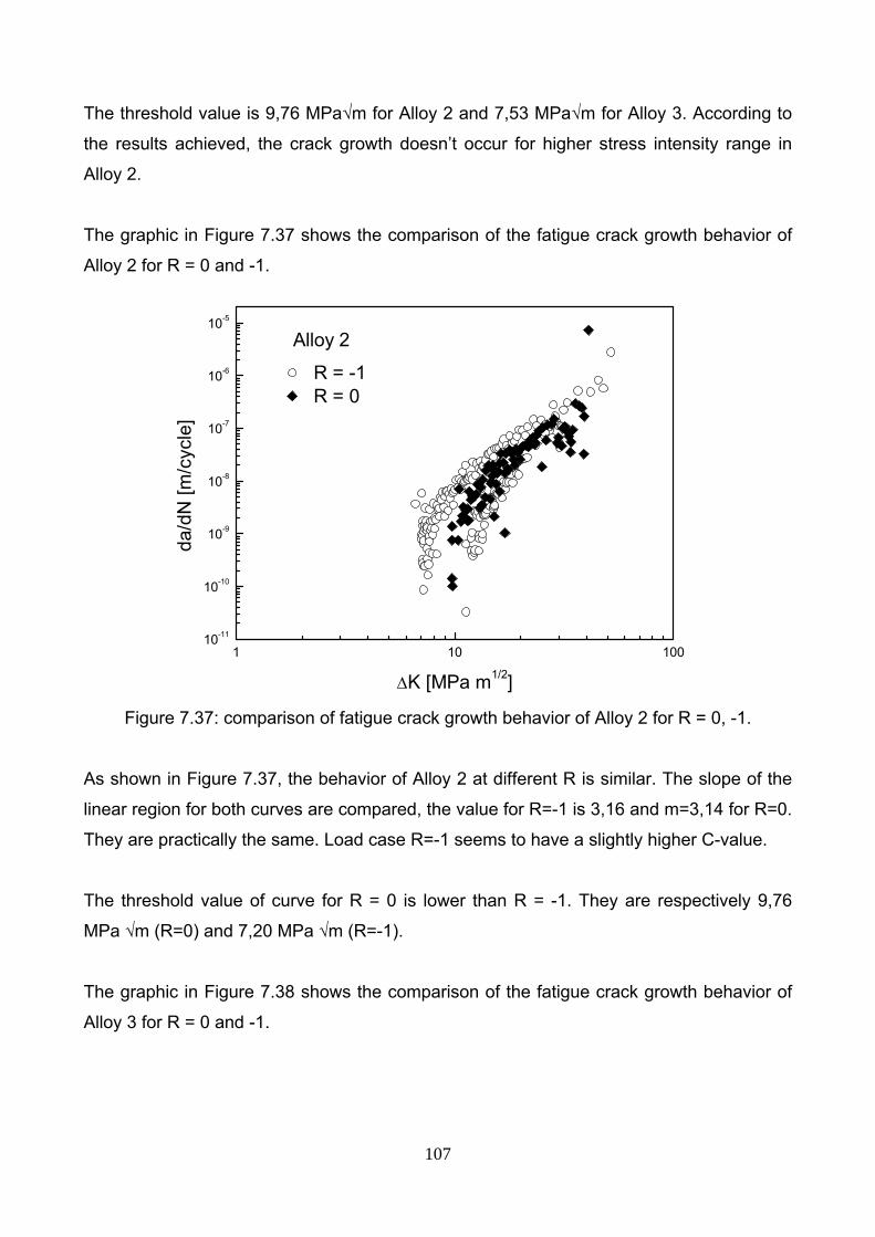
107
The threshold value is 9,76 MPa√m for Alloy 2 and 7,53 MPa√m for Alloy 3. According to
the results achieved, the crack growth doesn’t occur for higher stress intensity range in
Alloy 2.
The graphic in Figure 7.37 shows the comparison of the fatigue crack growth behavior of
Alloy 2 for R = 0 and -1.
1 10 10010-11
10-10
10-9
10-8
10-7
10-6
10-5
R = -1R = 0
da/d
N [m
/cyc
le]
ΔK [MPa m1/2]
Alloy 2
Figure 7.37: comparison of fatigue crack growth behavior of Alloy 2 for R = 0, -1.
As shown in Figure 7.37, the behavior of Alloy 2 at different R is similar. The slope of the
linear region for both curves are compared, the value for R=-1 is 3,16 and m=3,14 for R=0.
They are practically the same. Load case R=-1 seems to have a slightly higher C-value.
The threshold value of curve for R = 0 is lower than R = -1. They are respectively 9,76
MPa √m (R=0) and 7,20 MPa √m (R=-1).
The graphic in Figure 7.38 shows the comparison of the fatigue crack growth behavior of
Alloy 3 for R = 0 and -1.
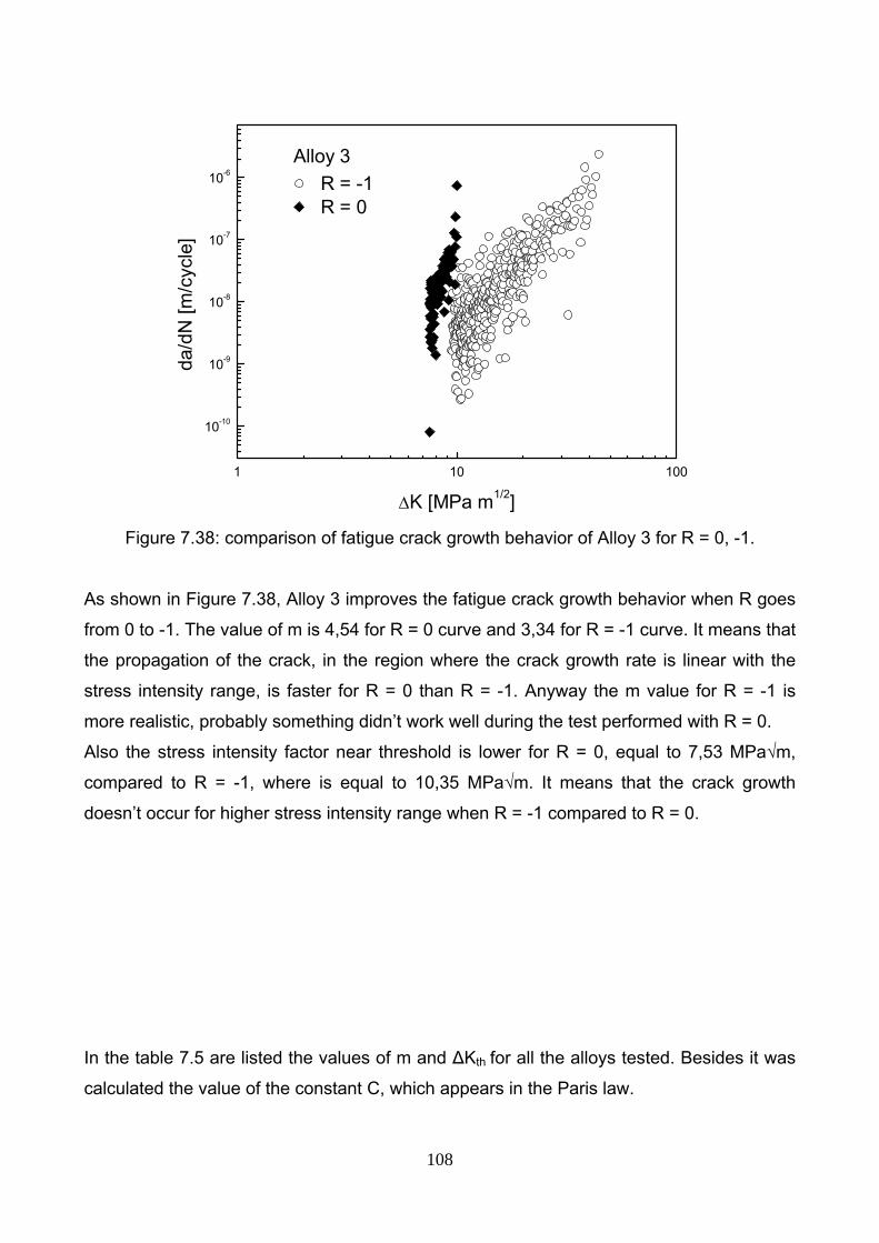
108
1 10 100
10-10
10-9
10-8
10-7
10-6
R = -1R = 0
da/d
N [m
/cyc
le]
ΔK [MPa m1/2]
Alloy 3
Figure 7.38: comparison of fatigue crack growth behavior of Alloy 3 for R = 0, -1.
As shown in Figure 7.38, Alloy 3 improves the fatigue crack growth behavior when R goes
from 0 to -1. The value of m is 4,54 for R = 0 curve and 3,34 for R = -1 curve. It means that
the propagation of the crack, in the region where the crack growth rate is linear with the
stress intensity range, is faster for R = 0 than R = -1. Anyway the m value for R = -1 is
more realistic, probably something didn’t work well during the test performed with R = 0.
Also the stress intensity factor near threshold is lower for R = 0, equal to 7,53 MPa√m,
compared to R = -1, where is equal to 10,35 MPa√m. It means that the crack growth
doesn’t occur for higher stress intensity range when R = -1 compared to R = 0.
In the table 7.5 are listed the values of m and ΔKth for all the alloys tested. Besides it was
calculated the value of the constant C, which appears in the Paris law.

109
Material R m C ΔKth [MPa√m]
-1 3,16 6,3 x10⁻¹² 7,20 Alloy 2
0 3,14 2,4 x10⁻¹² 9,76
-1 3,34 2,6 x10⁻¹² 10,35 Alloy 3
0 4,54 1,4 x10⁻¹² 7,53
Table 7.5: summary of values of m, C and ΔKth for Alloy 2 and 3.
As described before, the value of m raises when R increases from -1 to 0 for Alloy 3, and it
is similar for Alloy 2. It means that the crack propagates faster for R = 0 than R = -1, at
least in Alloy 3. It must be specified however, that the value measured for Alloy 3 with R =
0 is not realistic compared to the literature. Comparing the different alloys, Alloy 2 shows
slower crack propagation (lower values of m that means lower slopes) than Alloy 3.
However, considering the m value of Alloy 3 R = 0 less realistic, and the shape of the
curve of Alloy 2 R = -1 that shows two branches, the difference between the slope of all
the curves is not so large.
On the other hand, ΔKth decreases when R passes from -1 to 0 in Alloy 3, and increases in
Alloy 2. It means that the crack growth doesn’t occur for higher stress intensity range when
R is equal to 0 compared to -1 in Alloy 3, and the opposite happens in Alloy 2. However,
more investigations must be implemented for Alloy 3 load case R = 0. Moreover, Alloy 2
has lower values of ΔKth for R = -1, but higher for R = 0. In both cases, the results are not
completely clear: in order to the presence of the two branches in the Alloy 2 curve for R = -
1 due to pearlite formation and the not realistic results achieved for Alloy 3 R = 0 test, it’s
hard to conclude which one has the lower stress intensity range near threshold value.
Fracture surface analysis

110
Some of the specimens after the FCGR tests were analyzed by Light Optical Microscope
(LOM) and by Scanning Electron Microscopy (SEM).
Figure 7.39: fracture surface of Alloy 2 respectively near the notch and on the opposite
side.
Figure 7.40: fracture surface of Alloy 3 respectively near the notch and on the opposite
side.
It can be noticed from the Figures 7.39 and 7.40 that, for both the materials, there are
numerous small cracks beyond the main crack which brought to failure. As shown in the
images, those cracks are smaller near the notch (low ΔK) compare to the opposite side of
the sample, where the main crack is propagating (higher ΔK). These smaller cracks
develop mainly in the plastic zone that surround the main crack. Initiation spots seem to
bee the scattered isolate micro shrinkages and the graphite nodules. Interesting to
observe is that the number of secondary cracks increases in number as the stress
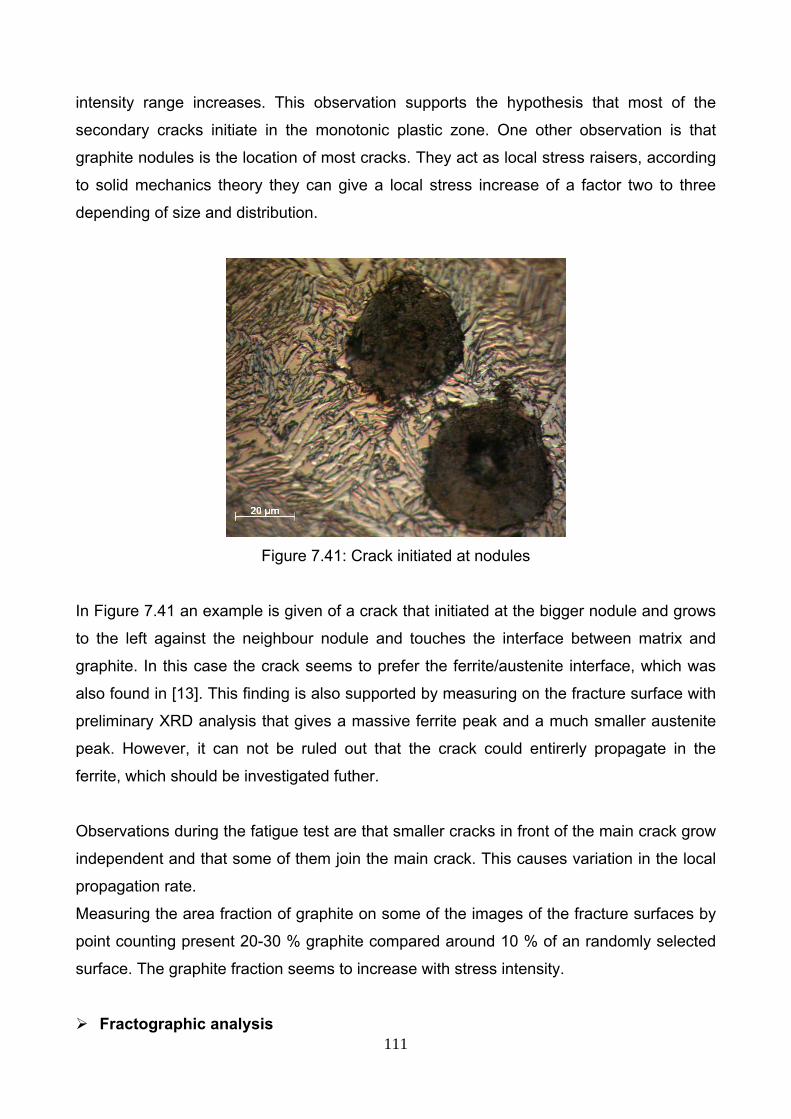
111
intensity range increases. This observation supports the hypothesis that most of the
secondary cracks initiate in the monotonic plastic zone. One other observation is that
graphite nodules is the location of most cracks. They act as local stress raisers, according
to solid mechanics theory they can give a local stress increase of a factor two to three
depending of size and distribution.
Figure 7.41: Crack initiated at nodules
In Figure 7.41 an example is given of a crack that initiated at the bigger nodule and grows
to the left against the neighbour nodule and touches the interface between matrix and
graphite. In this case the crack seems to prefer the ferrite/austenite interface, which was
also found in [13]. This finding is also supported by measuring on the fracture surface with
preliminary XRD analysis that gives a massive ferrite peak and a much smaller austenite
peak. However, it can not be ruled out that the crack could entirerly propagate in the
ferrite, which should be investigated futher.
Observations during the fatigue test are that smaller cracks in front of the main crack grow
independent and that some of them join the main crack. This causes variation in the local
propagation rate.
Measuring the area fraction of graphite on some of the images of the fracture surfaces by
point counting present 20-30 % graphite compared around 10 % of an randomly selected
surface. The graphite fraction seems to increase with stress intensity.
Fractographic analysis

112
An investigation of the fracture surface of some of the FCGR specimens was carried out
by Scanning Electron Microscope (SEM), in order to obtain a deeper analysis of the
phenomena that takes place during crack propagation.
Figure 7.42: A general overview of fracture surface at low ΔK.
Fracture surface in Figure 7.42 represents a good average of what happens at low ΔK
levels. Features that seems to guide the crack through the microstructure is shrinkages,
graphite nodules and cell boundaries. All these features determine both crack initiation
and how the crack chooses its path. Figure 7.42 shows a section around a cell boundary.
It appears that the porosity and the cell border graphite initiate the fracture. There are also
occasional cleavage facets. A normal fracture surface is ductile. This is clearly visible on
the traces of the needles in ausferrite shown in Figure 7.43.

113
Figure 7.43: close-up of fracture surface, can be clearly seen the needles and can be
recognized the ductile fracture.
Figure 7.44: close-up of a ductile fracture with nodules.
Figure 7.44 shows that there is a small plastic activity around the nodules, this is typical of
fatigue. It is also clear that there is an increased amount of graphite nodules on fracture
surface, including detachment of nodules. This suggests that nodules govern the fracture
process. The small picture on the left also shows that a cell boundary with the graphite
particles and a very small suction.
It can be seen in Figure 7.45 that the nodules seem to be intimately linked to the matrix, so
there are large number nodules that is "broken". Besides, it could be noticed that the

114
fracture area, especially at low ΔK, show less topography compared to fracture surfaces at
higher stress intensities.
Figure 7.45: broken nodules and damaged "flattened" areas.
When ΔK increases, the number of secondary cracks increases in number (Figure 7.46). It
is interesting to notice that these cracks are main cracks along the growth direction, but
they seem to go down into the test specimen.
Figure 7.46: secondary crack between nodules, the arrow shows the main crack growth
direction.
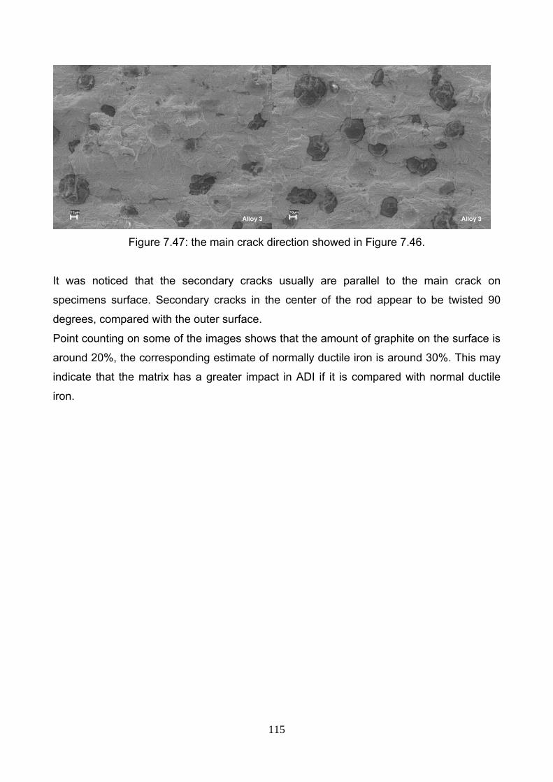
115
Figure 7.47: the main crack direction showed in Figure 7.46.
It was noticed that the secondary cracks usually are parallel to the main crack on
specimens surface. Secondary cracks in the center of the rod appear to be twisted 90
degrees, compared with the outer surface.
Point counting on some of the images shows that the amount of graphite on the surface is
around 20%, the corresponding estimate of normally ductile iron is around 30%. This may
indicate that the matrix has a greater impact in ADI if it is compared with normal ductile
iron.

116
8. CONCLUSION
The aim of the study was to evaluate the impact and the fatigue properties of
Austempered Ductile Iron.
The impact energy was found to be related with the morphology of graphite nodules.
Improved impact properties were obtained when the nodularity and the nodule count
increased. On the other hand, the impact energy decreased when the nodule size
increased. However in this work, the effect of the amount of retained austenite was found
to be less important than the graphite nodules. Moreover, the impact properties are
strongly affected by the defects like porosity, carbides and segregation mainly, but, also
the formation of martensite. They are the cause of the scattering achieved in the impact
energies and explain the lower values obtained in the middle location of the rings.
From investigating the fracture mechanism that occurs in ADI, it was observed that the
crack path preferentially intersects the graphite nodules. This is also a possible
explanation why the graphite nodules were more important for the fracture mechanism
than the retained austenite, which was also observe for the impact test. In this work, the
most dangerous crack initiator was found to be the pores, but also the carbides and the
nodule/matrix interface. The decrease of properties associated to the debonding of
graphite nodules is made easier with nodule size increases.
It was observed that the crack growth between two neighboring nodules depends on the
orientation of the ferrite laths. In fact the crack growth can take place along the
austenite/ferrite interface or cut the ferrite laths. In this work, it was found that the crack
path probably takes place along the austenite/ferrite interface, but this should be
investigated further.
For the fatigue test, faster crack propagation was found for R = 0 than R = -1 in Alloy 3
and similar in Alloy 2. However, the value measured for Alloy 3 with R = 0 is not consistent
to that found in literature in terms of m value. Comparing the different alloys, the difference
between the slope of all the curves is not so large. Alloy 2 shows slower crack propagation
than Alloy 3, despite of Alloy 2 at R = -1 had a curve shape with two branches.

117
On the other hand, ΔKth decreases when R passes from -1 to 0 in Alloy 3, and increases in
Alloy 2. It means that the crack growth doesn’t occur for higher stress intensity range when
R is equal to -1 compared to 0 in Alloy 3, and the opposite happens in Alloy 2. Comparing
different alloys at the same load case, Alloy 3 has higher threshold value than Alloy 2 for R
= -1, and lower for R = 0. Although, the results are not completely clear: the formaton of
pearlite affected the test, it should not be present in ADI and this is probably due to some
error in the casting process.
The fracture surface analysis of fatigue samples showed that the number of secondary
cracks increases in number as the stress intensity range increases. Besides, the graphite
nodules are the location of most cracks, due to the local stress increase.
Observations during the fatigue test are that smaller cracks in front of the main crack grow
independent and that some of them join the main crack. This causes variation in the local
propagation rate.
Measuring the area fraction of graphite on some of the mages of the fracture surfaces by
point counting present 20-30 % graphite compared around 10 % of an randomly selected
surface. The graphite fraction seems to increase with stress intensity.

118
9. REFERENCES
[1] E. Dorazil, High strength Austempered Ductile Cast Iron, Ellis Horwood series,
translation editor: H. Morrogh, 1991
[2] http://www.durhamfoundry.com/austempered_ductile_iron.htm
[3] http://www.aditreatments.com/background.php
[4] J. Hidalgo, Improving the Fracture Toughness of Dual-phase Austempered Ductile Iron,
Master Thesis, Department of Material and Manufacturing Technology, Chalmers
University of Technology, Göteborg, Sweden 2008, Chalmers Tekniska Högskola ISSN
1652-8913
[5] C.Glondu, Improving the Toughness of Austempered Ductile Iron, Master Thesis,
Department of Material and Manufacturing Technology, Chalmers University of
Technology, Göteborg, Sweden 2007, Chalmers Tekniska Högskola ISSN 1652-8913
[6] http://www.ductile.org/didata/section4/4intro.htm
[7] http://www.aditreatments.com/applications.php
[8] Y. Tanaka, H. Kage, Mater. Trans. JIM
[9] B. V. Kovacs, Modern Casting, 1990
[10] S. K. Putatunda, P. K. Gadicherla, Effect of Austempering Time on Mechanical
Properties of a Low Manganese Austempered Ductile Iron, Department of Chemical
Engineering and Materials Science, Wayne State University, Detroit, Journal of Materials
Engineering and Performance, vol. 9(2), pp. 193-203, 2000
[11] http://www.advancedcast.com/austempering-process.htm
[12] C.-K. Lin, P.-K. Lai, T.-S. Shih, Influence of microstructure on the fatigue properties of
austempered ductile irons-I. High-cycle fatigue, Department of Mechanical Engineering,
National Central University, Taiwan, International Journal of Fatigue vol. 18, No. 5, pp.
297-307, 1996
[13] C.-K. Lin, T.-P. Hung, Influence of microstructure on the fatigue properties of
austempered ductile irons-II. Low-cycle fatigue, Department of Mechanical Engineering,
National Central University, Taiwan, International Journal of Fatigue vol. 18, No. 5, pp.
309-320, 1996
[14] C.-K. Lin, Y.-L. Pai, Low-cycle fatigue of austempered ductile irons at various strain
ratios, Department of Mechanical Engineering, National Central University, Taiwan,
International Journal of Fatigue vol. 21, No. 1, pp. 45-54, 1999

119
[15] G. L. Greno, J. L. Otegui, R. E. Boeri, Mechanism of fatigue crack growth in
Austempered Ductile Iron, University of Mar de la Plata, Argentina, International Journal of
Fatigue vol. 21, No. 1, pp. 35-43, 1999
[16] M. D. Chapetti, High-cycle fatigue of austempered ductile iron (ADI), INTEMA
(Institute for Materials Science and Technology), CONICET-University of Mar de la Plata,
Argentina, International Journal of Fatigue vol. 29, pp. 860-868, 2007
[17] B. Stokes, N. Gao, K. K. Lee, P. A. S. Reed, Effects of Carbides on Fatigue
Characteristics of Austempered Ductile Iron, University of Southampton, UK, Metallurgical
and Materials Transactions A, vol. 36A, pp. 977-988, 2005
[18] M. Cavallini, O. Di Bartolomeo, F. Iacovello, Fatigue crack propagation damaging
micromechanism in ductile cast irons, University of Roma La Sapienza and Cassino, Italy,
Engineering Fracture Mechanics, vol. 75, pp.694-704, 2008
[19] C.-K. Lin, C.-W. Chang, Influence of heat treatment on fatigue crack of austempered
ductile iron, Department of Mechanical Engineering, National Central University, Taiwan,
Journal of Materials Science, vol. 37, pp. 709-716, 2002
[20] J. Luo, R. A. Harding, P. Bowen, Evaluation of Fatigue Behavior of Ductile Irons with
Various Matrix Microstructures, University of Birmingham, UK, Metallurgical and Materials
Transactions A, vol. 33A, pp. 3719-3730, 2002
[21] P. P. Rao, S. K. Putatunda, Influence of Microstructure on Fracture Toughness of
Austempered Ductile Iron, Department of Chemical Engineering and Materials Science,
College of Engineering, Wayne State University, Detroit, Metallurgical and Materials
Transactions A, vol. 28A, pp. 1457-1470, 1997
[22] G. Francucci, J. Sikora, R. Dommarco, Abrasion resistance of ductile iron
austempered by the two-step process, University of Mar de la Plata, INTEMA, CONICET,
Argentina, Materials Science and Engineering A, vol. 485, pp. 46-54, 2008
[23] I. Riposan, M. Chisamera, L. Sofroni, Cast Met., 1990, vol. 2, pp. 207-213
[24] R. C. Voigt, C. R. Loper, Proc. 1st Int. Conf. on Austempered Ductile Iron, Chicago,
1984
[25] R. C. Voigt, Ph. D. Thesis, University of Winsconsin-Madison, 1981
[26] E. V. Pereloma, C. S. Anderson, Microstructure and properties of austempered ductile
iron subjected to single and two step processing, Department of Materials Engineering,
Monash University, Victoria, Australia, Materials Science and Technology, vol. 22, No. 9,
pp. 1112-1118, 2006
120
[27] S. K. Putatunda, P. V. Gadicherla, Effect of Austempering Time on Mechanical
Properties of a Low Manganese Austempered Ductile Iron, Department of Chemical
Engineering and Materials Science, College of Engineering, Wayne State University,
Detroit, Journal of Materials Engineering an Performance, vol. 9, pp.193-203, 2000
[28] ASTM Handbooks, volume 4 Heat treating, section Quenching media for
austempering
[29] ASTM Handbooks, volume 4 Heat treating, section Equipment and Processing
[30] ASTM Handbooks, volume 4 Heat treating of Ductile Irons, section Quenching and
Tempering Ductile Iron
[31] L. Pook, Metal Fatigue: what it is, why it matters, Solid Mechanics and its
Applications, vol. 145, Springer, 2007
[32] J. Schijve, Fatigue of Structures and Materials, Kluwer Academic Publishers, 2001
[33] R. I. Stephens, A. Fatemi, R. R. Stephens, H. O. Fuchs, Metal Fatigue in Engineering,
John Wiley & Sons, Second Edition, 2001
[34] G. I. Rees, H. K. D. H. Bhadeshia, Material Science and Technology, vol. 8, pp. 985-
993, 1992
[35] N. A. Chester, H. K. D. H. Bhadeshia, Journal of Physics IV, vol. 7. C5, pp. 41-46,
1997
[36] E. V. Pereloma, S. H. Zahiri, C. H. J. Davies, Material Science and Technology,
vol.17, pp. 1563-1568, 2001
[37] E. V. Pereloma, S. H. Zahiri, C. H. J. Davies, Material Science and Technology,
vol.18, pp. 1163-1167, 2002
[38] M. Delia, M. Alaalam, M. Grech, Effect of Austenitizing Conditions on the Impact
Properties of an Alloyed Austempered Ductile Iron of Initially Ferritic Matrix Structure,
Department of Metallurgy and Materials, Faculty of Engineering, University of Malta,
Journal of Materials Engineering and Performance, vol. 7(2), pp.265-272, 1998
[39] O. Erić, M. Jovanović, L. Šidanin, D. Rajnović, S. Zec, The austempering study of
alloyed ductile iron, Materials and design, vol. 27, pp. 617-622, 2006
[40] Bayati, Elliott, Materials Science and Technology, 11:285, 1995
[41] Hamid Ali AS, Uzolov KI, Darwish N, Elliott R, Materials Science and Technology,
10:35, 1994
[42] T. Skaland, D. Grog, Nodule Distribution in Ductile Cast Iron, AFS Trans., vol. 56, pp.
153-157, 1991

121
[43] B.Y. Lin, E.T. Chen, T.S. Lei, The Effect of Segregation on the Austemper
Transformation and Toughness of Ductile Irons, Department of Mechanical Engineering
and Technology, National Taiwan Institute of Technology, Taipei, Taiwan, Journal of
Materials Engineering and Performance, vol. 7(3), pp. 407-419, 1998
[44] C. S. Roberts, Trans AIME, 1953, vol. 197 pp.203-206
[45] H. Bayati, R. Elliott, Austempering process in high-manganese alloyed ductile cast
iron, Mat. Sci. Tech., 11, 284-293 (1995)
[46] K. Hamberg, Microstructural Influence on the Fatigue Properties of Steels,
Department of Engineering Metals, Chalmers University of Technology, Göteborg,
Sweden 1986

122