HAL Id: inria-00548302https://hal.inria.fr/inria-00548302

Submitted on 22 Dec 2010

HAL is a multi-disciplinary open accessarchive for the deposit and dissemination of sci-entific research documents, whether they are pub-lished or not. The documents may come fromteaching and research institutions in France orabroad, or from public or private research centers.

L’archive ouverte pluridisciplinaire HAL, estdestinée au dépôt et à la diffusion de documentsscientifiques de niveau recherche, publiés ou non,émanant des établissements d’enseignement et derecherche français ou étrangers, des laboratoirespublics ou privés.

Evaluation of Interest Point DetectorsCordelia Schmid, Roger Mohr, Christian Bauckhage

To cite this version:Cordelia Schmid, Roger Mohr, Christian Bauckhage. Evaluation of Interest Point Detec-tors. International Journal of Computer Vision, Springer Verlag, 2000, 37 (2), pp.151–172.�10.1023/A:1008199403446�. �inria-00548302�

Evaluation of Interest Point DetectorsCordelia Schmid, Roger Mohr and Christian BauckhageINRIA Rhone-Alpes655 av. de l'Europe38330 Montbonnot, FranceCordelia.Schmid@inrialpes.fr

1

KeywordsInterest Points, Quantitative Evaluation, Comparison of Detectors, Repeatability, InformationContent

2

AbstractMany di�erent low-level feature detectors exist and it is widely agreed that the evaluation ofdetectors is important. In this paper we introduce two evaluation criteria for interest points :repeatability rate and information content. Repeatability rate evaluates the geometric stabilityunder di�erent transformations. Information content measures the distinctiveness of features.Di�erent interest point detectors are compared using these two criteria. We determine whichdetector gives the best results and show that it satis�es the criteria well.

3

1 IntroductionMany computer vision tasks rely on low-level features. A wide variety of feature detectorsexist, and results can vary enormously depending on the detector used. It is widely agreedthat evaluation of feature detectors is important [36]. Existing evaluation methods use ground-truth veri�cation [5], visual inspection [20, 27], localization accuracy [3, 6, 8, 22], theoreticalanalysis [11, 15, 40] or speci�c tasks [45, 46].In this paper we introduce two novel criteria for evaluating interest points : repeatability andinformation content. Those two criteria directly measure the quality of the feature for tasks likeimage matching, object recognition and 3D reconstruction. They apply to any type of scene,and they do not rely on any speci�c feature model or high-level interpretation of the feature.Our criteria are more general than most existing evaluation methods (cf. section 1.1). Theyare complementary to localization accuracy which is relevant for tasks like camera calibrationand 3D reconstruction of speci�c scene points. This criterion has previously been evaluated forinterest point detectors [3, 6, 8, 22].Repeatability explicitly compares the geometrical stability of the detected interest points be-tween di�erent images of a given scene taken under varying viewing conditions. Previous methodshave evaluated detectors for individual images only. An interest point is \repeated", if the 3Dscene point detected in the �rst image is also accurately detected in the second one. The repeata-bility rate is the percentage of the total observed points that are detected in both images. Notethat repeatability and localization are con icting criteria - smoothing improves repeatability butdegrades localization [7].Information content is a measure of the distinctiveness of an interest point. Distinctivenessis based on the likelihood of a local greyvalue descriptor computed at the point within thepopulation of all observed interest point descriptors. Descriptors characterize the local shapeof the image at the interest points. The entropy of these descriptors measures the informationcontent of a set of interest points.In this paper several detectors are compared using these two evaluation criteria. The best4

detector satis�es both of these criteria well, which explains its success for tasks such as imagematching based on interest points and correlation [49]. In this context at least a subset of thepoints have to be repeated in order to allow feature correspondence. Furthermore, if image-basedmeasures (e.g. correlation) are used to compare points, interest points should have distinctivepatterns.1.1 Related work on the evaluation of feature detectorsThe evaluation of feature detectors has concentrated on edges. Only a few authors have evaluatedinterest point detectors. In the following we give a few examples of existing edge evaluationmethods and a survey of previous work on evaluating interest points. Existing methods canbe categorized into methods based on : ground-truth veri�cation, visual inspection, localizationaccuracy, theoretical analysis and speci�c tasks.1.1.1 Ground-truth veri�cationMethods based on ground-truth veri�cation determine the undetected features and the falsepositives. Ground-truth is in general created by a human. It relies on his symbolic interpretationof the image and is therefore subjective. Furthermore, human interpretation limits the complexityof the images used for evaluation.For example, Bowyer et al [5] use human marked ground-truth to evaluate edge detectors.Their evaluation criterion is the number of false positives with respect to the number of un-matched edges which is measured for varying input parameters. They used structured outdoorscenes, such as airports and buildings.1.1.2 Visual inspectionMethods using visual inspection are even more subjective as they are directly dependent on thehuman evaluating the results. L�opez et al [27] de�ne a set of visual criteria to evaluate thequality of detection. They visually compare a set of ridge and valley detectors in the context ofmedical images. Heath et al [20] evaluate detectors using a visual rating score which indicates5

the perceived quality of the edges for identifying an object. This score is measured by a groupof people. Di�erent edge detectors are evaluated on real images of complex scenes.1.1.3 Localization accuracyLocalization accuracy is the criterion most often used to evaluate interest points. It measureswhether an interest point is accurately located at a speci�c 2D location. This criterion is sig-ni�cant for tasks like camera calibration and the 3D reconstruction of speci�c scene points.Evaluation requires the knowledge of precise 3D properties, which restricts the evaluation tosimple scenes.Localization accuracy is often measured by verifying that a set of 2D image points is coherentwith the known set of corresponding 3D scene points. For example Coehlo et al [8] compare thelocalization accuracy of interest point detectors using di�erent planar projective invariants forwhich reference values are computed using scene measurements. The scene contains simple blackpolygons and is imaged from di�erent viewing angles. A similar evaluation scheme is used byHeyden and Rohr [22]. They extract sets of points from images of polyhedral objects and useprojective invariants to compute a manifold of constraints on the points.Brand and Mohr [6] measure the localization accuracy of a model-based L-corner detector.They use four di�erent criteria : alignment of the extracted points, accuracy of the 3D recon-struction, accuracy of the epipolar geometry and stability of the cross-ratio. Their scene is againvery simple : it contains black squares on a white background.To evaluate the accuracy of edge point detectors, Baker and Nayar [3] propose four globalcriteria : collinearity, intersection at a single point, parallelism and localization on an ellipse. Eachof the criteria corresponds to a particular (very simple) scene and is measured using the extractededgels. Their experiments are conducted under widely varying image conditions (illuminationchange and 3D rotation).As mentioned by Heyden and Rohr, methods based on projective invariants don't require theknowledge of the exact position of the features in the image. This is an advantage of suchmethods, as the location of features in an image depends both on the intrinsic parameters of6

the camera and the relative position and orientation of the object with respect to the cameraand is therefore di�cult to determine. However, the disadvantage of such methods is the lack ofcomparison to true data which may introduce a systematic bias.1.1.4 Theoretical analysisMethods based on a theoretical analysis examine the behavior of the detectors for theoreticalfeature models. Such methods are limited, as they only apply to very speci�c features. For exam-ple, Deriche and Giraudon [15] study analytically the behavior of three interest point detectorsusing a L-corner model. Their study allows them to correct the localization bias. Rohr [40]performs a similar analysis for L-corners with aperture angles in the range of 0 and 180 degrees.His analysis evaluates 10 di�erent detectors.Demigny and Kaml�e [11] use three criteria to theoretically evaluate four step edge detectors.Their criteria are based on Canny's criteria which are adapted to the discrete domain usingsignal processing theory. Canny's criteria are good detection, good localization and low responsesmultiplicity.1.1.5 A speci�c taskA few methods have evaluated detectors through speci�c tasks. They consider that featuredetection is not a �nal result by itself, but merely an input for further processing. Therefore, thetrue performance criterion is how well it prepares the input for the next algorithm. This is nodoubt true to some extent. However, evaluations based on a speci�c task and system are hardto generalize and hence rather limited.Shin et al [45] compare edge detectors using an object recognition algorithm. Test images arecars imaged under di�erent lighting conditions and in front of varying backgrounds. In Shin etal [46] the performance of a edge-based structure from motion algorithm is used for evaluation.Results are given for two simple 3D scenes which are imaged under varying 3D rotations.7

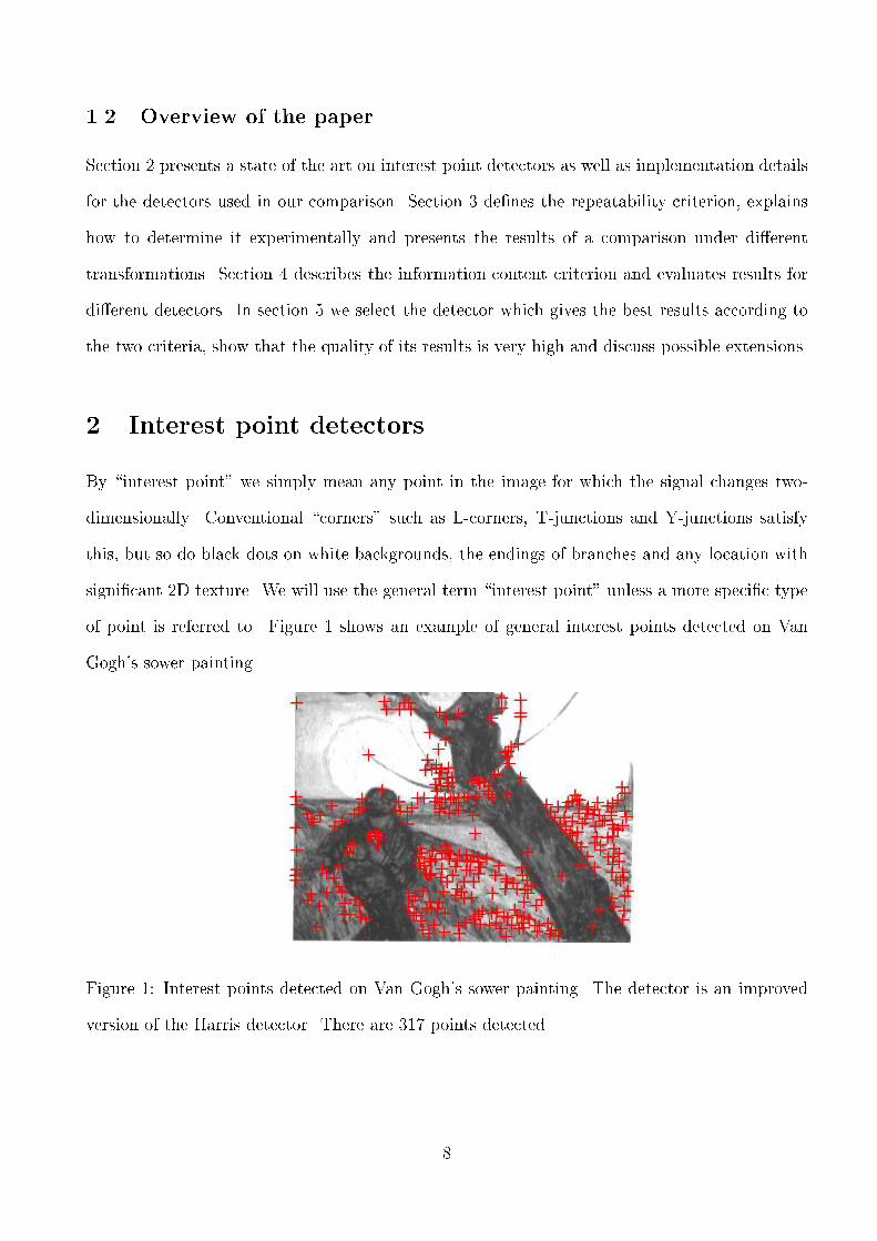
1.2 Overview of the paperSection 2 presents a state of the art on interest point detectors as well as implementation detailsfor the detectors used in our comparison. Section 3 de�nes the repeatability criterion, explainshow to determine it experimentally and presents the results of a comparison under di�erenttransformations. Section 4 describes the information content criterion and evaluates results fordi�erent detectors. In section 5 we select the detector which gives the best results according tothe two criteria, show that the quality of its results is very high and discuss possible extensions.2 Interest point detectorsBy \interest point" we simply mean any point in the image for which the signal changes two-dimensionally. Conventional \corners" such as L-corners, T-junctions and Y-junctions satisfythis, but so do black dots on white backgrounds, the endings of branches and any location withsigni�cant 2D texture. We will use the general term \interest point" unless a more speci�c typeof point is referred to. Figure 1 shows an example of general interest points detected on VanGogh's sower painting.

Figure 1: Interest points detected on Van Gogh's sower painting. The detector is an improvedversion of the Harris detector. There are 317 points detected.8

2.1 State of the artA wide variety of interest point and corner detectors exist in the literature. They can be dividedinto three categories : contour based, intensity based and parametric model based methods. Con-tour based methods �rst extract contours and then search for maximal curvature or in exionpoints along the contour chains, or do some polygonal approximation and then search for inter-section points. Intensity based methods compute a measure that indicates the presence of aninterest point directly from the greyvalues. Parametric model methods �t a parametric intensitymodel to the signal. They often provide sub-pixel accuracy, but are limited to speci�c types ofinterest points, for example to L-corners. In the following we brie y present detection methodsfor each of the three categories.2.1.1 Contour based methodsContour based methods have existed for a long time ; some of the more recent ones are presented.Asada and Brady [1] extract interest points for 2D objects from planar curves. They observe thatthese curves have special characteristics : the changes in curvature. These changes are classi�edin several categories : junctions, endings etc. To achieve robust detection, their algorithm isintegrated in a multi-scale framework. A similar approach has been developed by Mokhtarianand Mackworth [29]. They use in exion points of a planar curve.Medioni and Yasumoto [28] use B-splines to approximate the contours. Interest points aremaxima of curvature which are computed from the coe�cients of these B-splines.Horaud et al [23] extract line segments from the image contours. These segments are groupedand intersections of grouped line segments are used as interest points.Shilat et al [44] �rst detect ridges and troughs in the images. Interest points are high curvaturepoints along ridges or troughs, or intersection points. They argue that such points are moreappropriate for tracking, as they are less likely to lie on the occluding contours of an object.Mokhtarian and Suomela [30] describe an interest point detector based on two sets of interestpoints. One set are T-junctions extracted from edge intersections. A second set is obtained usinga multi-scale framework : interest points are curvature maxima of contours at a coarse level and9

are tracked locally up to the �nest level. The two sets are compared and close interest pointsare merged.The algorithm of Pikaz and Dinstein [37] is based on a decomposition of noisy digital curvesinto a minimal number of convex and concave sections. The location of each separation pointis optimized, yielding the minimal possible distance between the smoothed approximation andthe original curve. The detection of the interest points is based on properties of pairs of sectionsthat are determined in an adaptive manner, rather than on properties of single points that arebased on a �xed-size neighborhood.2.1.2 Intensity based methodsMoravec [31] developed one of the �rst signal based interest point detectors. His detector is basedon the auto-correlation function of the signal. It measures the greyvalue di�erences between awindow and windows shifted in several directions. Four discrete shifts in directions parallel tothe rows and columns of the image are used. If the minimum of these four di�erences is superiorto a threshold, an interest point is detected.The detector of Beaudet [4] uses the second derivatives of the signal for computing the measure\DET" : DET = IxxIyy � I2xy where I(x; y) is the intensity surface of the image. DET is thedeterminant of the Hessian matrix and is related to the Gaussian curvature of the signal. Thismeasure is invariant to rotation. Points where this measure is maximal are interest points.Kitchen and Rosenfeld [24] present an interest point detector which uses the curvature of planarcurves. They look for curvature maxima on isophotes of the signal. However, due to image noisean isophote can have an important curvature without corresponding to an interest point, forexample on a region with almost uniform greyvalues. Therefore, the curvature is multiplied bythe gradient magnitude of the image where non-maximum suppression is applied to the gradientmagnitude before multiplication. Their measure is K = IxxI2y+IyyI2x�2IxyIxIyI2x+I2y .Dreschler and Nagel [16] �rst determine locations of local extrema of the determinant of theHessian \DET". A location of maximum positive DET can be matched with a location ofextreme negative DET , if the directions of the principal curvatures which have opposite sign10

are approximatively aligned. The interest point is located between these two points at the zerocrossing of DET . Nagel [32] shows that the Dreschler-Nagel's approach and Kitchen-Rosenfeld'sapproach are identical.Several interest point detectors [17, 18, 19, 48] are based on a matrix related to the auto-correlation function. This matrix A averages derivatives of the signal in a window W around apoint (x; y) : A(x; y) = 266664 P(xk ;yk)2W(Ix(xk; yk))2 P(xk;yk)2W Ix(xk; yk)Iy(xk; yk)P(xk ;yk)2W Ix(xk; yk)Iy(xk; yk) P(xk;yk)2W(Iy(xk; yk))2 377775 (1)where I(x; y) is the image function and (xk; yk) are the points in the window W around (x; y).This matrix captures the structure of the neighborhood. If this matrix is of rank two, that isboth of its eigenvalues are large, an interest point is detected. A matrix of rank one indicatesan edge and a matrix of rank zero a homogeneous region. The relation between this matrix andthe auto-correlation function is given in appendix A.Harris [19] improves the approach of Moravec by using the auto-correlation matrix A. Theuse of discrete directions and discrete shifts is thus avoided. Instead of using a simple sum, aGaussian is used to weight the derivatives inside the window. Interest points are detected if theauto-correlation matrix A has two signi�cant eigenvalues.F�orstner and G�ulch [18] propose a two step procedure for localizing interest points. Firstpoints are detected by searching for optimal windows using the auto-correlation matrix A. Thisdetection yields systematic localization errors, for example in the case of L-corners. A secondstep based on a di�erential edge intersection approach improves the localization accuracy.F�orstner [17] uses the auto-correlation matrix A to classify image pixels into categories - region,contour and interest point. Interest points are further classi�ed into junctions or circular featuresby analyzing the local gradient �eld. This analysis is also used to determine the interest pointlocation. Local statistics allow a blind estimate of signal-dependent noise variance for automaticselection of thresholds and image restoration.Tomasi and Kanade [48] motivate their approach in the context of tracking. A good feature11

is de�ned as one that can be tracked well. They show that such a feature is present if theeigenvalues of matrix A are signi�cant.Heitger et al [21] develop an approach inspired by experiments on the biological visual system.They extract 1D directional characteristics by convolving the image with orientation-selectiveGabor like �lters. In order to obtain 2D characteristics, they compute the �rst and secondderivatives of the 1D characteristics.Cooper and al [9] �rst measure the contour direction locally and then compute image di�erencesalong the contour direction. A knowledge of the noise characteristics is used to determine whetherthe image di�erences along the contour direction are su�cient to indicate an interest point. Earlyjump-out tests allow a fast computation of the image di�erences.The detector of Reisfeld et al [38] uses the concept of symmetry. They compute a symmetrymap which shows a \symmetry strength" for each pixel. This symmetry is computed locally bylooking at the magnitude and the direction of the derivatives of neighboring points. Points withhigh symmetry are selected as interest points.Smith and Brady [47] compare the brightness of each pixel in a circular mask to the centerpixel to de�ne an area that has a similar brightness to the center. Two dimensional features canbe detected from the size, centroid and second moment of this area.The approach proposed by Lagani�ere [26] is based on a variant of the morphological closingoperator which successively applies dilation/erosion with di�erent structuring elements. Twoclosing operators and four structuring elements are used. The �rst closing operator is sensitiveto vertical/horizontal L-corners and the second to diagonal L-corners.2.1.3 Parametric model based methodsThe parametric model used by Rohr [39] is an analytic junction model convolved with a Gaussian.The parameters of the model are adjusted by a minimization method, such that the templateis closest to the observed signal. In the case of a L-corner the parameters of the model are theangle of the L-corner, the angle between the symmetry axis of the L-corner and the x-axis, thegreyvalues, the position of the point and the amount of blur. Positions obtained by this method12

are very precise. However, the quality of the approximation depends on the initial positionestimation. Rohr uses an interest point detector which maximizes det(A) (cf. equation (1)) aswell as the intersection of line segments to determine the initial values for the model parameters.Deriche and Blaszka [14] develop an acceleration of Rohr's method. They substitute an ex-ponential for the Gaussian smoothing function. They also show that to assure convergence theimage region has to be quite large. In cluttered images the region is likely to contain severalsignals, which makes convergence di�cult.Baker et al [2] propose an algorithm that automatically constructs a detector for an arbitraryparametric feature. Each feature is represented as a densely sampled parametric manifold in a lowdimensional subspace. A feature is detected, if the projection of the surrounding intensity valuesin the subspace lies su�ciently close to the feature manifold. Furthermore, during detection theparameters of detected features are recovered using the closest point on the feature manifold.Parida et al [34] describe a method for general junction detection. A deformable templateis used to detect radial partitions. The minimum description length principle determines theoptimal number of partitions that best describes the signal.2.2 Implementation detailsThis section presents implementation details for the detectors included in our comparison. Thedetectors are Harris [19], an improved version of Harris, Cottier[10], Horaud [23], Heitger [21]and F�orstner [17]. Except in the case of the improved version of Harris, we have used the imple-mentations of the original authors, with the standard default parameter values recommended bythe authors for general purpose feature detection. These values are seldom optimal for any givenimage, but they do well on average on collections of di�erent images. Our goal is to evaluatedetectors for such collections.The standard Harris detector [19] (\Harris") computes the derivatives of the matrix A (cf.equation (1)) by convolution with the mask [ -2 -1 0 1 2 ]. A Gaussian (� = 2) is used to weightthe derivatives summed over the window. To avoid the extraction of the eigenvalues of the matrixA, the strength of an interest points is measured by det(A)�� trace(A)2. The second term is used13

to eliminate contour points with a strong eigenvalue, � is set to 0:06. Non-maximum suppressionusing a 3x3 mask is then applied to the interest point strength and a threshold is used to selectinterest points. The threshold is set to 1% of the maximum observed interest point strength.In the improved version of Harris (\ImpHarris"), derivatives are computed more preciselyby replacing the [ -2 -1 0 1 2 ] mask with derivatives of a Gaussian (� = 1). A recursiveimplementation of the Gaussian �lters [13] guarantees fast detection.Cottier [10] applies the Harris detector only to contour points in the image. Derivatives forcontour extraction as well as for the Harris detector are computed by convolution with theCanny/Deriche operator [12] (� = 2, ! = 0:001). Local maxima detection with hysteresisthresholding is used to extract contours. High and low thresholds are determined from thegradient magnitude (high = average gradient magnitude, low = 0.1 * high). For the Harrisdetector derivatives are averaged over two di�erent window sizes in order to increase localizationaccuracy. Points are �rst detected using a 5x5 window. The exact location is then determinedby using a 3x3 window and searching the maximum in the neighborhood of the detected point.Horaud [23] �rst extracts contour chains using his implementation of the Canny edge detector.Tangent discontinuities in the chain are located using a worm, and a line �t between the dis-continuities is estimated using orthogonal regression. Lines are then grouped and intersectionsbetween neighboring lines are used as interest points.Heitger [21] convolves the image with even and odd symmetrical orientation-selective �lters.These Gabor like �lters are parameterized by the width of the Gaussian envelope (� =5), thesweep which increases the relative weight of the negative side-lobes of even �lters and the orien-tation selectivity which de�nes the sharpness of the orientation tuning. Even and odd �lters arecomputed for 6 orientations. For each orientation an energy map is computed by combining evenand odd �lter outputs. 2D signal variations are then determined by di�erentiating each energymap along the respective orientation using \end-stopped operators". Non-maximum suppression(3x3 mask) is applied to the combined end-stopped operator activity and a relative threshold(0.1) is used to select interest points.The F�orstner detector [17] computes the derivatives on the smoothed image (� = 0:7). The14

derivatives are then summed over a Gaussian window (� = 2) to obtain the auto-correlationmatrix A. The trace of this matrix is used to classify pixels into region or non-region. For ho-mogeneous regions the trace follows approximatively a �2-distribution. This allows to determinethe classi�cation threshold automatically using a signi�cance level (� = 0.95) and the estimatednoise variance. Pixels are further classi�ed into contour or interest point using the ratio of theeigenvalues and a �xed threshold (0.3). Interest point locations are then determined by mini-mizing a function of the local gradient �eld. The parameter of this function is the size of theGaussian which is used to compute a weighted sum over the local gradient measures (� = 4).3 Repeatability3.1 Repeatability criterionRepeatability signi�es that detection is independent of changes in the imaging conditions, i.e. theparameters of the camera, its position relative to the scene, and the illumination conditions. 3Dpoints detected in one image should also be detected at approximately corresponding positionsin subsequent ones (cf. �gure 2). Given a 3D point X and two projection matrices P1 and Pi,the projections of X into images I1 and Ii are x1 = P1X and xi = PiX. A point x1 detected inimage I1 is repeated in image Ii if the corresponding point xi is detected in image Ii. To measurethe repeatability, a unique relation between x1 and xi has to be established. This is di�cult forgeneral 3D scenes, but in the case of a planar scene this relation is de�ned by a homography [42] :xi = H1ix1 where H1i = PiP�11P�11 is an abusive notation to represent the back-projection of image I1. In the case of a planarscene this back-projection exists.The repeatability rate is de�ned as the number of points repeated between two images withrespect to the total number of detected points. To measure the number of repeated points, wehave to take into account that the observed scene parts di�er in the presence of changed imagingconditions, such as image rotation or scale change. Interest points which can not be observed in15

x1

X

O1 Oi

P1 iP

I1

xi

I i

H1i

ε

Figure 2: The points x1 and xi are the projections of 3D pointX into images I1 and Ii : x1 = P1Xand xi = PiX where P1 and Pi are the projection matrices. A detected point x1 is repeated if xiis detected. It is �-repeated if a point is detected in the �-neighborhood of xi. In case of planarscenes the points x1 and xi are related by the homography H1i.both images corrupt the repeatability measure. Therefore only points which lie in the commonscene part are used to compute the repeatability. This common scene part is determined by thehomography. Points ~x1 and ~xi which lie in the common part of images I1 and Ii are de�ned by :f~x1g = fx1 j H1ix1 2 Iig and f~xig = fxi j Hi1xi 2 I1gwhere fx1g and fxig are the points detected in images I1 and Ii respectively. Hij is the homog-raphy between images Ii and Ij.Furthermore, the repeatability measure has to take into account the uncertainty of detection. Arepeated point is in general not detected exactly at position xi, but rather in some neighborhoodof xi. The size of this neighborhood is denoted by � (cf. �gure 2) and repeatability within thisneighborhood is called �-repeatability. The set of point pairs (~x1; ~xi) which correspond within an�-neighborhood is de�ned by :Ri(�) = f(~x1; ~xi) j dist(H1i~x1; ~xi) < �gThe number of detected points may be di�erent for the two images. In the case of a scalechange, for example, more interest points are detected on the high resolution image. Only theminimum number of interest points (the number of interest points of the coarse image) can be16

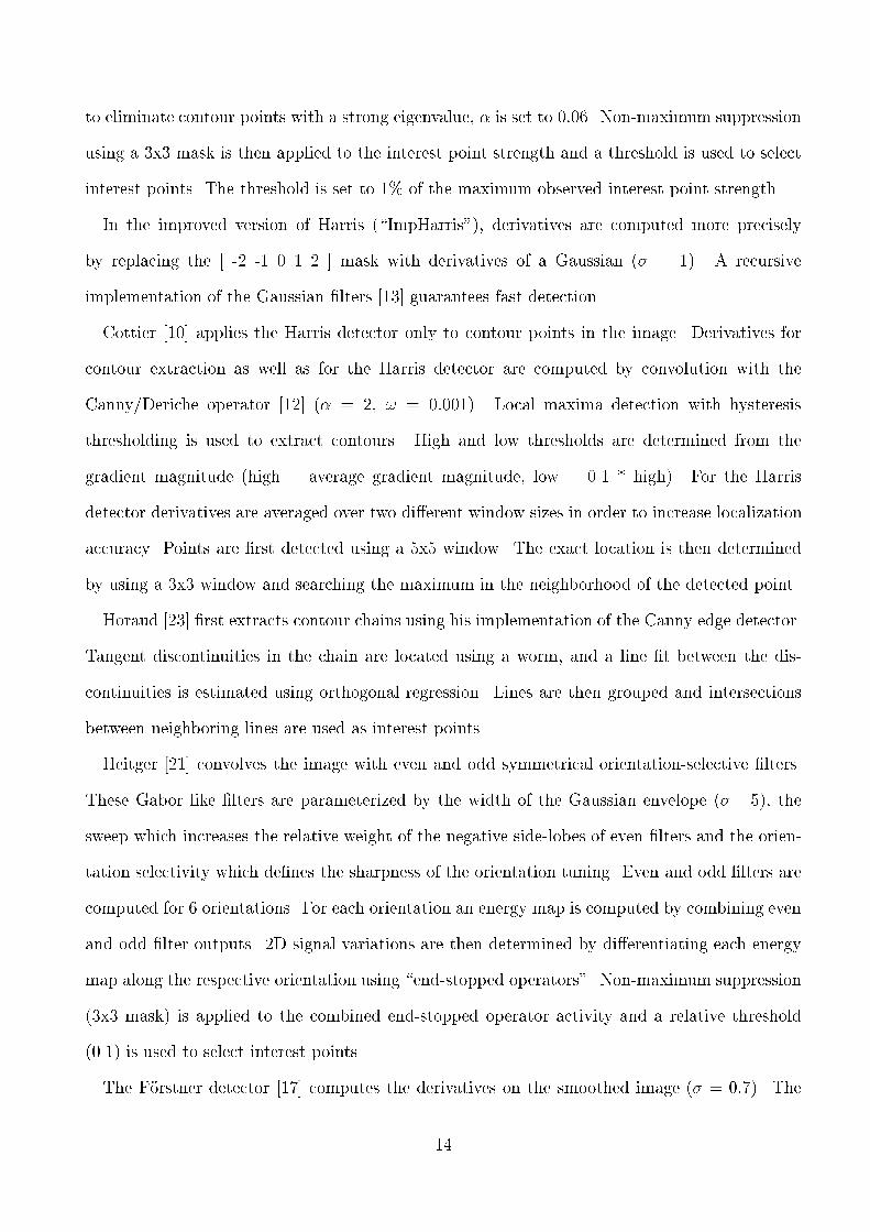
repeated. The repeatability rate ri(�) for image Ii is thus de�ned by :ri(�) = jRi(�)jmin (n1; ni)where n1 = jf~x1gj and ni = jf~xigj are the number of points detected in the common part ofimages I1 and Ii respectively. We can easily verify that 0 � ri(�) � 1.The repeatability criterion, as de�ned above, is only valid for planar scenes. Only for suchscenes the geometric relation between two images is completely de�ned. However, the restrictionto planar scenes is not a limitation, as additional interest points detected on 3D scenes are dueto occlusions and shadows. These points are due to real changes of the observed scene and therepeatability criterion should not take into account such unreliable points [43, 44].3.2 Experimental conditionsSequences The repeatability rates of several interest point detectors are compared under di�er-ent transformations : image rotation, scale change, illumination variation and viewpoint change.We consider both uniform and complex illumination variation. Stability to image noise has alsobeen tested. The scene is always static and we move either the camera or the light source.We will illustrate results for two planar scenes : \Van Gogh" and \Asterix". The \Van Gogh"scene is the sower painting shown in �gure 1. The \Asterix" scene can be seen in �gure 3. Thetwo scenes are very di�erent : the \Van Gogh" scene is highly textured whereas the \Asterix"scene is mostly line drawings.Estimating the homography To ensure an accurate repeatability rate, the computation ofthe homography has to be precise and independent of the detected points. An independent, sub-pixel localization is required. We therefore take a second image for each position of the camera,with black dots projected onto the scene (cf. �gure 3). The dots are extracted very preciselyby �tting a template, and their centers are used to compute the homography. A least mediansquare method makes the computation robust.While recording the sequence, the scene and the projection mechanism (overhead projector)17

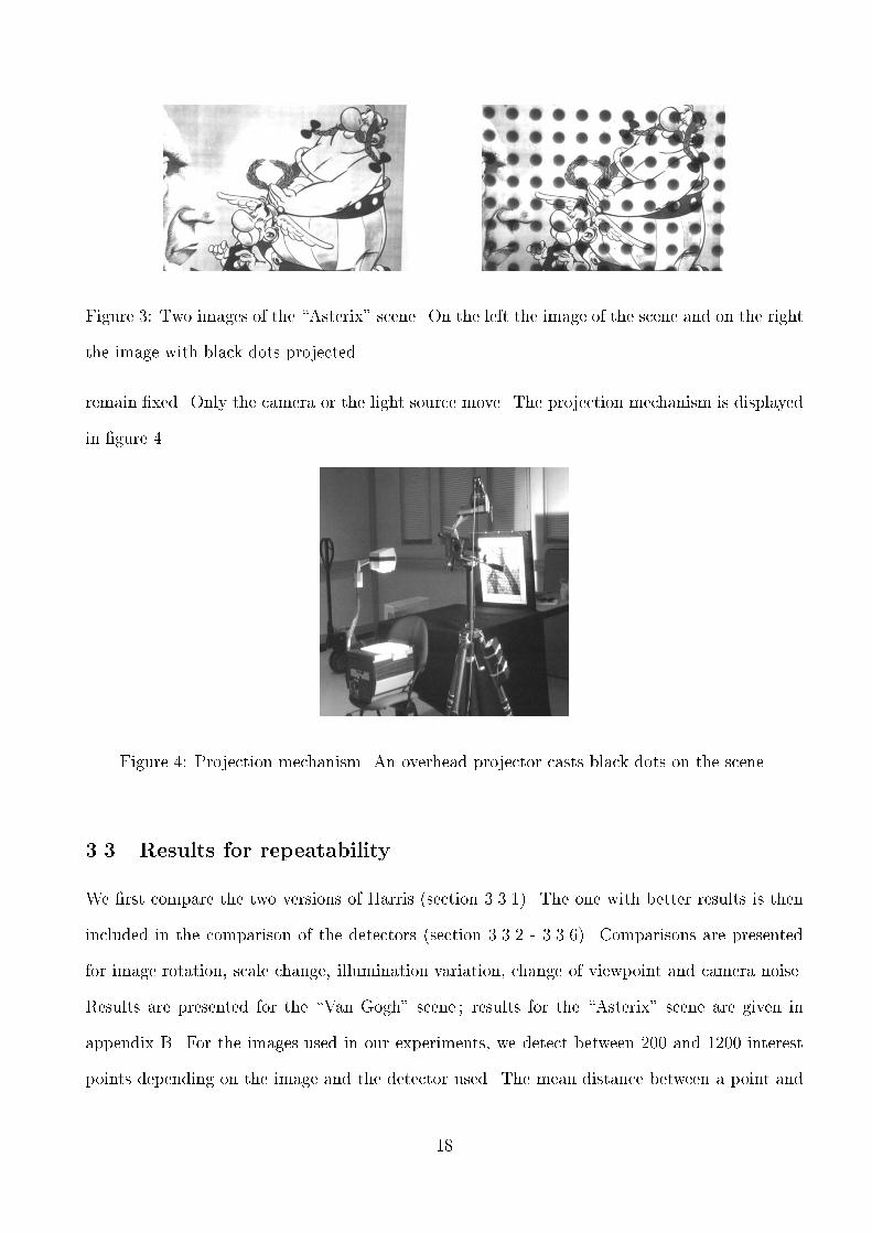
Figure 3: Two images of the \Asterix" scene. On the left the image of the scene and on the rightthe image with black dots projected.remain �xed. Only the camera or the light source move. The projection mechanism is displayedin �gure 4.

Figure 4: Projection mechanism. An overhead projector casts black dots on the scene.3.3 Results for repeatabilityWe �rst compare the two versions of Harris (section 3.3.1). The one with better results is thenincluded in the comparison of the detectors (section 3.3.2 - 3.3.6). Comparisons are presentedfor image rotation, scale change, illumination variation, change of viewpoint and camera noise.Results are presented for the \Van Gogh" scene ; results for the \Asterix" scene are given inappendix B. For the images used in our experiments, we detect between 200 and 1200 interestpoints depending on the image and the detector used. The mean distance between a point and18

its closest neighbor is around 10 pixels. Measuring the repeatability rate with �=1.5 or less, theprobability that two points are accidentally within the error distance is very low.3.3.1 Comparison of the two Harris versionsFigure 5 compares the two di�erent versions of the Harris detector in the presence of imagerotation (graph on the left) and scale change (graph on the right). The repeatability of theimproved version of Harris (ImpHarris) is better in both cases. The results of the standardversion vary with image rotation, the worst results being obtained for an angle of 45�. This isdue to the fact that the standard version uses non-isotropic discrete derivative �lters. A stableimplementation of the derivatives signi�cantly improves the repeatability of the Harris detector.The improved version (ImpHarris) is included in the comparison of the detectors in the followingsections.

0

0.2

0.4

0.6

0.8

1

1.2

0 20 40 60 80 100 120 140 160 180

repe

atab

ility

rat

e

rotation angle in degrees

HarrisImpHarris

0

0.2

0.4

0.6

0.8

1

1 1.5 2 2.5 3 3.5 4 4.5

repe

atab

ility

rat

e

scale factor

HarrisImpHarris

Figure 5: Comparison of Harris and ImpHarris. On the left the repeatability rate for an imagerotation and on the right the rate for a scale change. � = 1.5.3.3.2 Image rotationIn this section, we compare all detectors described in section 2.2 for an image rotation. Imagerotations are obtained by rotating the camera around its optical axis using a special mechanism.Figure 6 shows three images of the rotation sequence. The left image is the reference image.The rotation angle for the image in the middle is 38� and for the image on the right 116�. The19

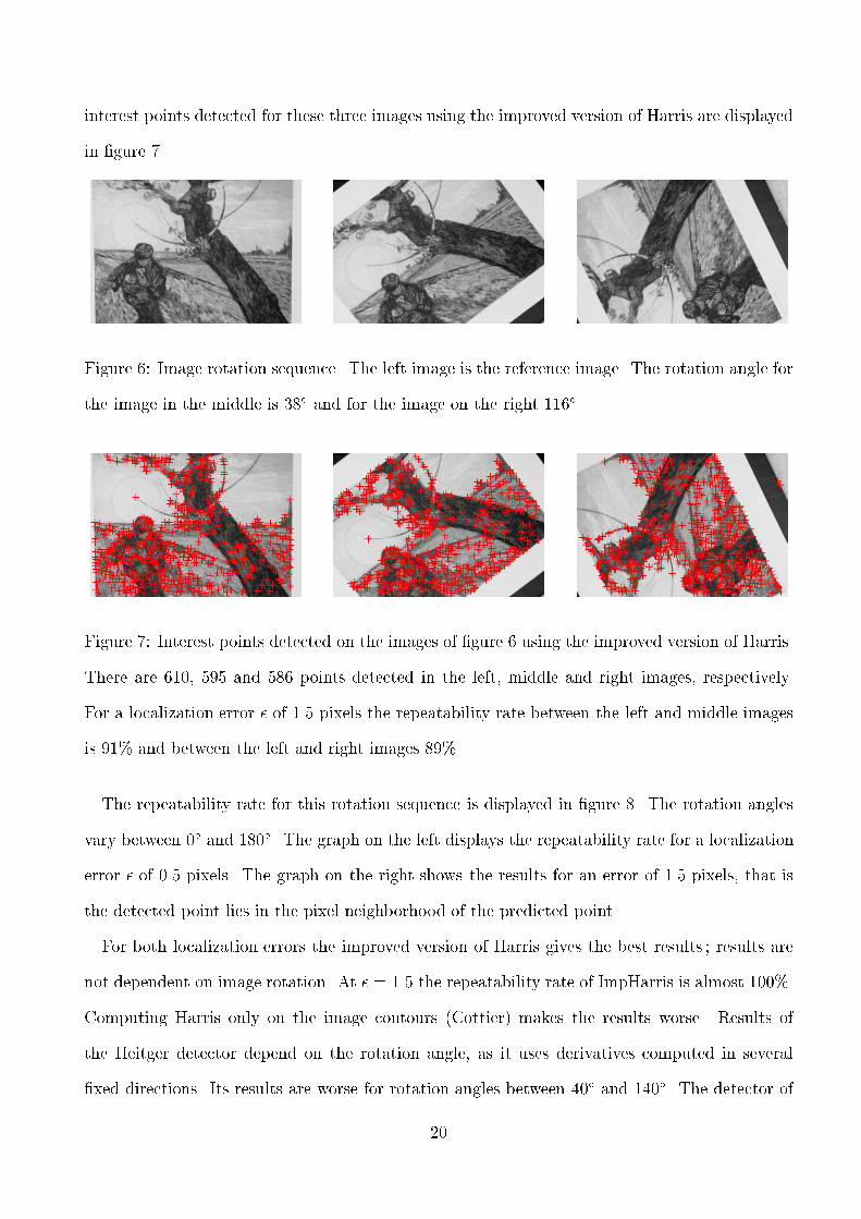
interest points detected for these three images using the improved version of Harris are displayedin �gure 7.Figure 6: Image rotation sequence. The left image is the reference image. The rotation angle forthe image in the middle is 38� and for the image on the right 116�.

Figure 7: Interest points detected on the images of �gure 6 using the improved version of Harris.There are 610, 595 and 586 points detected in the left, middle and right images, respectively.For a localization error � of 1.5 pixels the repeatability rate between the left and middle imagesis 91% and between the left and right images 89%The repeatability rate for this rotation sequence is displayed in �gure 8. The rotation anglesvary between 0� and 180�. The graph on the left displays the repeatability rate for a localizationerror � of 0.5 pixels. The graph on the right shows the results for an error of 1.5 pixels, that isthe detected point lies in the pixel neighborhood of the predicted point.For both localization errors the improved version of Harris gives the best results ; results arenot dependent on image rotation. At � = 1.5 the repeatability rate of ImpHarris is almost 100%.Computing Harris only on the image contours (Cottier) makes the results worse. Results ofthe Heitger detector depend on the rotation angle, as it uses derivatives computed in several�xed directions. Its results are worse for rotation angles between 40� and 140�. The detector of20

0

0.2

0.4

0.6

0.8

1

1.2

0 20 40 60 80 100 120 140 160 180

repe

atab

ility

rat

e

rotation angle in degrees

ImpHarrisFoerstner

CottierHeitgerHoraud

0

0.2

0.4

0.6

0.8

1

1.2

0 20 40 60 80 100 120 140 160 180

repe

atab

ility

rat

e

rotation angle in degrees

ImpHarrisFoerstner

CottierHeitgerHoraud

Figure 8: Repeatability rate for image rotation. � = 0.5 for the left graph and � = 1.5 for theright graph.F�orstner gives bad results for rotations of 45�, probably owing to the use of anisotropic derivative�lters. The worst results are obtained by the method based on the intersection of line segments(Horaud).Figure 9 shows the repeatability rate as a function of the localization error � for a constantrotation angle of 89 degrees. The localization error varies between 0.5 pixels and 5 pixels. Whenincreasing the localization error, the results improve for all the detectors. However, the improvedversion of Harris detector is always best and increases most rapidly. For this detector, good resultsare obtained above a 1 pixel localization error.

0

0.2

0.4

0.6

0.8

1

0 1 2 3 4 5

repe

atab

ility

rat

e

localization error

ImpHarrisFoerstner

CottierHeitgerHoraudFigure 9: Repeatability rate as a function of the localization error �. The rotation angle is 89�.

21

3.3.3 Scale changeScale change is investigated by varying the focal length of the camera. Figure 10 shows threeimages of the scale change sequence. The left image is the reference image. The scale changefor the middle one is 1.5 and for the right one 4.1. The scale factors have been determined bythe ratios of the focal lengths. The interest points detected for these three images using theimproved version of Harris are displayed in �gure 11.Figure 10: Scale change sequence. The left image is the reference image. The scale change forthe middle one is 1.5 and for the right one 4.1.

Figure 11: Interest points detected on the images of �gure 10 using the improved version of Harris.There are 317, 399 and 300 points detected in the left, middle and right images, respectively.The repeatability rate between the left and middle images is 54% and between the left and rightimages 1% for a localization error � of 1.5 pixels.Figure 12 shows the repeatability rate for scale changes. The left graph shows the repeatabilityrate for an � of 0.5 and the right one for an � of 1.5 pixels. Evidently the detectors are verysensitive to scale changes. For an � of 0.5 (1.5) repeatability is very poor for a scale factor above22

0

0.2

0.4

0.6

0.8

1

1 1.5 2 2.5 3 3.5 4 4.5

repe

atab

ility

rat

e

scale factor

ImpHarrisFoerstner

CottierHeitgerHoraud

0

0.2

0.4

0.6

0.8

1

1 1.5 2 2.5 3 3.5 4 4.5

repe

atab

ility

rat

e

scale factor

ImpHarrisFoerstner

CottierHeitgerHoraud

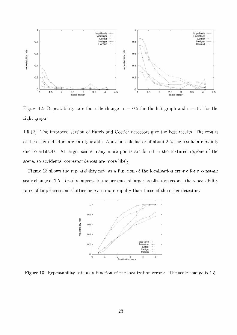
Figure 12: Repeatability rate for scale change. � = 0.5 for the left graph and � = 1.5 for theright graph.1.5 (2). The improved version of Harris and Cottier detectors give the best results. The resultsof the other detectors are hardly usable. Above a scale factor of about 2.5, the results are mainlydue to artifacts. At larger scales many more points are found in the textured regions of thescene, so accidental correspondences are more likely.Figure 13 shows the repeatability rate as a function of the localization error � for a constantscale change of 1.5. Results improve in the presence of larger localization errors ; the repeatabilityrates of ImpHarris and Cottier increase more rapidly than those of the other detectors.

0

0.2

0.4

0.6

0.8

1

0 1 2 3 4 5

repe

atab

ility

rat

e

localization error

ImpHarrisFoerstner

CottierHeitgerHoraudFigure 13: Repeatability rate as a function of the localization error �. The scale change is 1.5.

23

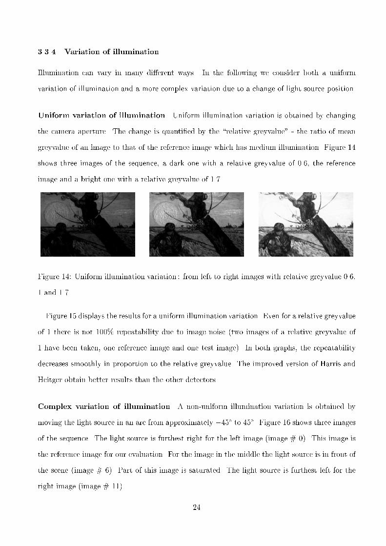
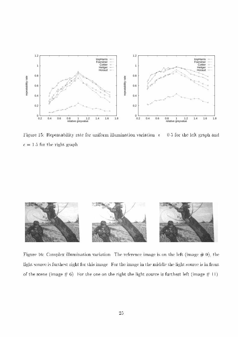
3.3.4 Variation of illuminationIllumination can vary in many di�erent ways. In the following we consider both a uniformvariation of illumination and a more complex variation due to a change of light source position.Uniform variation of illumination Uniform illumination variation is obtained by changingthe camera aperture. The change is quanti�ed by the \relative greyvalue" - the ratio of meangreyvalue of an image to that of the reference image which has medium illumination. Figure 14shows three images of the sequence, a dark one with a relative greyvalue of 0.6, the referenceimage and a bright one with a relative greyvalue of 1.7.Figure 14: Uniform illumination variation : from left to right images with relative greyvalue 0.6,1 and 1.7.Figure 15 displays the results for a uniform illumination variation. Even for a relative greyvalueof 1 there is not 100% repeatability due to image noise (two images of a relative greyvalue of1 have been taken, one reference image and one test image). In both graphs, the repeatabilitydecreases smoothly in proportion to the relative greyvalue. The improved version of Harris andHeitger obtain better results than the other detectors.Complex variation of illumination A non-uniform illumination variation is obtained bymoving the light source in an arc from approximately �45� to 45�. Figure 16 shows three imagesof the sequence. The light source is furthest right for the left image (image # 0). This image isthe reference image for our evaluation. For the image in the middle the light source is in front ofthe scene (image # 6). Part of this image is saturated. The light source is furthest left for theright image (image # 11). 24

0

0.2

0.4

0.6

0.8

1

1.2

0.2 0.4 0.6 0.8 1 1.2 1.4 1.6 1.8

repe

atab

ility

rat

e

relative greyvalue

ImpHarrisFoerstner

CottierHeitgerHoraud

0

0.2

0.4

0.6

0.8

1

1.2

0.2 0.4 0.6 0.8 1 1.2 1.4 1.6 1.8

repe

atab

ility

rat

erelative greyvalue

ImpHarrisFoerstner

CottierHeitgerHoraud

Figure 15: Repeatability rate for uniform illumination variation. � = 0.5 for the left graph and� = 1.5 for the right graph.

Figure 16: Complex illumination variation. The reference image is on the left (image # 0), thelight source is furthest right for this image. For the image in the middle the light source is in frontof the scene (image # 6). For the one on the right the light source is furthest left (image # 11).25

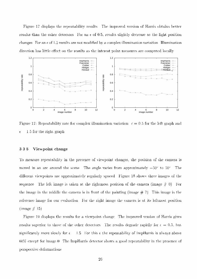
Figure 17 displays the repeatability results. The improved version of Harris obtains betterresults than the other detectors. For an � of 0:5, results slightly decrease as the light positionchanges. For an � of 1:5 results are not modi�ed by a complex illumination variation. Illuminationdirection has little e�ect on the results as the interest point measures are computed locally.

0

0.2

0.4

0.6

0.8

1

1.2

0 2 4 6 8 10 12

repe

atab

ility

rat

e

image number

ImpHarrisFoerstner

CottierHeitgerHoraud

0

0.2

0.4

0.6

0.8

1

1.2

0 2 4 6 8 10 12

repe

atab

ility

rat

e

image number

ImpHarrisFoerstner

CottierHeitgerHoraud

Figure 17: Repeatability rate for complex illumination variation. � = 0.5 for the left graph and� = 1.5 for the right graph.3.3.5 Viewpoint changeTo measure repeatability in the presence of viewpoint changes, the position of the camera ismoved in an arc around the scene. The angle varies from approximately �50� to 50�. Thedi�erent viewpoints are approximately regularly spaced. Figure 18 shows three images of thesequence. The left image is taken at the rightmost position of the camera (image # 0). Forthe image in the middle the camera is in front of the painting (image # 7). This image is thereference image for our evaluation. For the right image the camera is at its leftmost position(image # 15).Figure 19 displays the results for a viewpoint change. The improved version of Harris givesresults superior to those of the other detectors. The results degrade rapidly for � = 0:5, butsigni�cantly more slowly for � = 1:5. For this � the repeatability of ImpHarris is always above60% except for image 0. The ImpHarris detector shows a good repeatability in the presence ofperspective deformations. 26

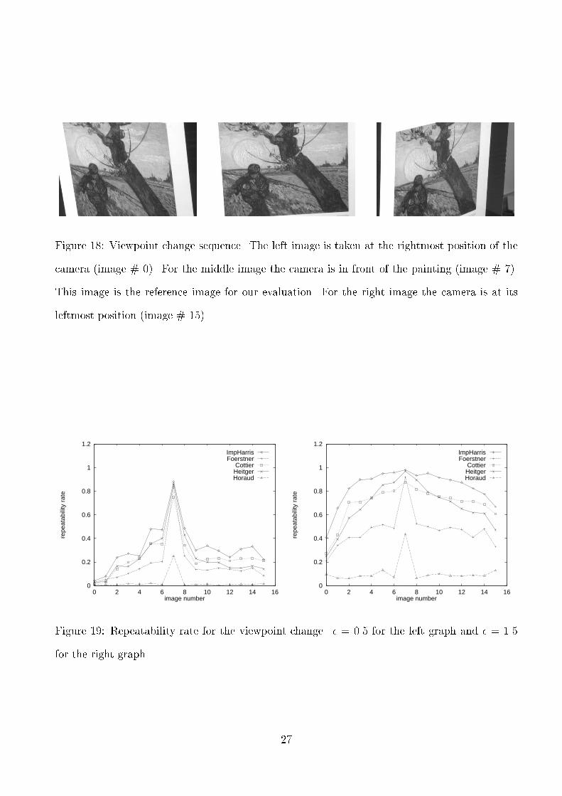
Figure 18: Viewpoint change sequence. The left image is taken at the rightmost position of thecamera (image # 0). For the middle image the camera is in front of the painting (image # 7).This image is the reference image for our evaluation. For the right image the camera is at itsleftmost position (image # 15).

0

0.2

0.4

0.6

0.8

1

1.2

0 2 4 6 8 10 12 14 16

repe

atab

ility

rat

e

image number

ImpHarrisFoerstner

CottierHeitgerHoraud

0

0.2

0.4

0.6

0.8

1

1.2

0 2 4 6 8 10 12 14 16

repe

atab

ility

rat

e

image number

ImpHarrisFoerstner

CottierHeitgerHoraud

Figure 19: Repeatability rate for the viewpoint change. � = 0.5 for the left graph and � = 1.5for the right graph.27

3.3.6 Camera noiseTo study repeatability in the presence of image noise, a static scene has been recorded severaltimes. The results of this experiment are displayed in �gure 20. We can see that all detectorsgive good results except the Horaud one. The improved version of Harris gives the best results,followed closely by Heitger. For � = 1:5 these two detectors obtain a rate of nearly 100%.

0

0.2

0.4

0.6

0.8

1

1.2

1 2 3 4 5 6 7 8 9

repe

atab

ility

rat

e

image number

ImpHarrisFoerstner

CottierHeitgerHoraud

0

0.2

0.4

0.6

0.8

1

1.2

1 2 3 4 5 6 7 8 9

repe

atab

ility

rat

e

image number

ImpHarrisFoerstner

CottierHeitgerHoraudFigure 20: Repeatability rate for the camera noise. � = 0.5 for the left graph and � = 1.5 for theright graph.

3.4 Conclusion for repeatabilityRepeatability of various detectors has been evaluated in the presence of di�erent imaging condi-tions : image rotation, scale change, variation of illumination, viewpoint change and noise of theimaging system. Two di�erent scenes have been used : "Van Gogh" and "Asterix". The resultsfor these two sequences are very similar ; the \Asterix" sequence (cf. appendix B) con�rms theresults presented above.Results of the previous section show that a stable implementation of the derivatives improvesthe results of the standard Harris detector. The improved version of Harris (ImpHarris) givessigni�cantly better results than the other detectors in the presence of image rotation. This is dueto the rotation invariance of its image measures. The detector of Heitger combines computationsin several directions and is not invariant to rotations. This is con�rmed by Perona [35] who has28

noticed that the computation in several directions is less stable to an image rotation. ImpHarrisand Cottier give the best results in the presence of scale changes. Moreover, the computation ofthese detectors is based on Gaussian �lters and can easily be adapted to scale changes. In thecase of illumination variations and camera noise, ImpHarris and Heitger obtain the best results.For a viewpoint change ImpHarris shows results which are superior to the other detectors.In all cases the results of the improved version of the Harris detector are better or equivalentto those of the other detectors. For this detector, interest points are largely independent of theimaging conditions ; points are geometrically stable.4 Information content4.1 Information content criterionInformation content is a measure of the distinctiveness of an interest point. Distinctivenessis based on the likelihood of a local greyvalue descriptor computed at the point within thepopulation of all observed interest point descriptors. Given one or several images, a descriptor iscomputed for each of the detected interest points. Information content measures the distributionof these descriptors. If all descriptors lie close together, they don't convey any information, thatis the information content is low. Matching for example fails, as any point can be matched toany other. On the other hand if the descriptors are spread out, information content is high andmatching is likely to succeed.Information content of the descriptors is measured using entropy. The more spread out thedescriptors are, the higher is the entropy. Section 4.2 presents a short introduction to entropyand shows that entropy measures the average information content. In section 4.3 we introducethe descriptors used for our evaluation, which characterize local greyvalue patterns. Section 4.4describes how to partition the set of descriptors. Partitioning of the descriptors is necessary tocompute the entropy, as will be explained in section 4.2. The information content criterion ofdi�erent detectors is compared in section 4.5. 29

4.2 EntropyEntropy measures the randomness of a variable. The more random a variable is the biggerthe entropy. In the following we are not going to deal with continuous variables, but withpartitions [33]. The entropy of a partition A = fAig is :H(A) = �Xi pi log(pi) (2)where pi is the probability of Ai.Note that the size of the partition in uences the results. If B is a new partition formed bysubdivisions of the sets of A then H(B) � H(A).Entropy measures average information content. In information theory the information contentI of a message i is de�ned as Ii = log(1=pi) = �log(pi)The information content of a message is inversely related to its probability. If pi = 1 the eventalways occurs and no information is attributed to it : I = 0. The average information contentper message of a set of messages is then de�ned by �Pi pi log(pi) which is its entropy.In the case of interest points we would like to know how much average information content aninterest point "transmits", as measured by its descriptor. The more distinctive the descriptorsare, the larger is the average information content.4.3 Descriptors characterizing local shapeTo measure the distribution of local greyvalue patterns at interest points, we have to de�ne ameasure which describes such patterns. Collecting unordered pixel values at an interest pointdoes not represent the shape of the signal around the pixel. Collecting ordered pixel values (e.g.from left to right and from top to bottom) respects the shape but is not invariant to rotation.We have therefore chosen to use local rotation invariants.The rotation invariants used are combinations of greyvalue derivatives. Greyvalue derivativesare computed stably by convolution with Gaussian derivatives. This set of derivatives is called30

the \local jet" [25]. Note that derivatives up to Nth order describe the intensity function locallyup to that order. The \local jet" of order N at a point x = (x; y) for image I and scale � isde�ned by : JN [I](x; �) = fLi1:::in(x; �) j (x; �) 2 I � IR+ ;n = 0; : : : ; Ngwhere Li1:::in(x; �) is the convolution of image I with the Gaussian derivatives Gi1:::in(x; �) andik 2 fx; yg.To obtain invariance under the group SO(2) (2D image rotations), Koenderink [25] andRomeny [41] compute di�erential invariants from the local jet. In our work invariants up tosecond order are used :~V[0::3] = 266666666664

LxLx + LyLyLxxLxLx + 2LxyLxLy + LyyLyLyLxx + LyyLxxLxx + 2LxyLxy + LyyLyy377777777775 (3)

The average luminance does not characterize the shape and is therefore not included. Note thatthe �rst component of ~V is the square of the gradient magnitude and the third is the Laplacian.4.4 Partitioning a set of descriptorsThe computation of entropy requires the partitioning of the descriptors ~V . Partitioning is de-pendent on the distance measure between descriptors. The distance between two descriptors ~V1and ~V2 is given by the Mahalanobis distance :dM(~V2; ~V1) = q(~V2 � ~V1)T��1(~V2 � ~V1)The covariance matrix � takes into account the variability of the descriptors ~V, i.e. their uncer-tainty due to noise. This matrix � is symmetric positive de�nite. Its inverse can be decomposedinto ��1 = P TDP where D is diagonal and P an orthogonal matrix representing a change ofreference frame. We can then de�ne the square root of ��1 as ��1=2 = D1=2P where D1=2 is adiagonal matrix whose coe�cients are the square roots of the coe�cients of D. The Mahalanobis31

distance can then be rewritten as :dM(~V2; ~V1) = kD1=2P (~V2 � ~V1)kThe distance dM is the norm of the di�erence of the normalized vectors :~Vnorm = D1=2P ~V (4)Normalization allows us to use equally sized cells in all dimensions. This is important since theentropy is directly dependent on the partition used. The probability of each cell of this partitionis used to compute the entropy of a set of vectors ~V.4.5 Results for information contentIn this section, we compute the information content of the detectors which are included in ourcomparison. To obtain a statistically signi�cant measure, a large number of points has to beconsidered. We use a set of 1000 images of di�erent types : aerial images, images of paintingsand images of toy objects. The information content of a detector is computed as follows :1. Extract interest points for the set of images.2. Compute descriptors (cf. equation (3)) for all extracted interest points (�=3).3. Normalize each descriptor (cf. equation (4)). The covariance matrix takes into account thevariability of the descriptors.4. Partition the set of normalized descriptors. The cell size is the same in all dimensions, itis set to 20.5. Determine the probability of each cell and compute the entropy with equation (2).The results are presented in table 1. It shows that the improved version of Harris producesthe highest entropy, and hence the most distinctive points. The results obtained for Heitger arealmost as good. The two detectors based on line extraction obtain worse results. This can be32

explained by their limitation to contour lines which reduces the distinctiveness of their greyvaluedescriptors and thus their entropy.Random points are included in our comparison : for each image we compute the mean numberm of interest points extracted by the di�erent detectors. We then select m random pointsover the image using a spatially uniform distribution. Entropy is computed as speci�ed aboveusing this random point detector. The result for this detector (\random") is given in table 1.Unsurprisingly, the results obtained for all of the interest point detectors are signi�cantly betterthan those for random points. The probability to produce a collision is e�(3:3�6:05) � 15:6 timeshigher for Random than for Harris.detector information contentImpHarris 6.049526Heitger 5.940877Horaud 5.433776Cottier 4.846409F�orstner 4.523368Random 3.300863Table 1: The information content for di�erent detectors.5 ConclusionIn this paper we have introduced two novel evaluation criteria : repeatability and informationcontent. These two criteria present several advantages over existing ones. First of all, they aresigni�cant for a large number of computer vision tasks. Repeatability compares interest pointsdetected on images taken under varying viewing conditions and is therefore signi�cant for anyinterest point based algorithm which uses two or more images of a given scene. Examples areimage matching, geometric hashing, computation of the epipolar geometry etc.Information content is relevant for algorithms which use greyvalue information. Examples33

are image matching based on correlation and object recognition based on local feature vectors.Furthermore, repeatability as well as information content are independent of human interventionand apply to real scenes.The two criteria have been used to evaluate and compare several interest point detectors.Repeatability was evaluated under various di�erent imaging conditions. In all cases the improvedversion of Harris is better than or equivalent to those of the other detectors. Except for largescale changes, its points are geometrically stable under all tested image variations. The resultsfor information content again show that the improved version of Harris obtains the best results,although the Heitger detector is a close second. All of the detectors have signi�cantly higherinformation content than randomly selected points, so they do manage to select \interesting"points.The criteria de�ned in this paper allow the quantitative evaluation of new interest point de-tectors. One possible extension is to adapt these criteria to other low-level features. Anotherextension would be to design an improved interest point detector with respect to the two eval-uation criteria. Concerning repeatability, we have seen that detectors show rapid degradationin the presence of scale change. To solve this problem, the detectors could be included in amulti-scale framework. Another solution might be to estimate the scale at which the best resultsare obtained. Concerning information content, we think that studying which kinds of greyvaluedescriptors occur frequently and which ones are rare will help us to design a detector with evenhigher information content.AcknowledgmentsWe are very grateful to Yves Dufournaud, Radu Horaud and Andrew Zisserman for discussions.

34

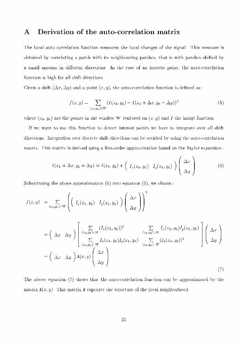
A Derivation of the auto-correlation matrixThe local auto-correlation function measures the local changes of the signal. This measure isobtained by correlating a patch with its neighbouring patches, that is with patches shifted bya small amount in di�erent directions. In the case of an interest point, the auto-correlationfunction is high for all shift directions.Given a shift (�x;�y) and a point (x; y), the auto-correlation function is de�ned as :f(x; y) = X(xk;yk)2W(I(xk; yk)� I(xk +�x; yk +�y))2 (5)where (xk; yk) are the points in the window W centered on (x; y) and I the image function.If we want to use this function to detect interest points we have to integrate over all shiftdirections. Integration over discrete shift directions can be avoided by using the auto-correlationmatrix. This matrix is derived using a �rst-order approximation based on the Taylor expansion :I(xk +�x; yk +�y) � I(xk; yk) + � Ix(xk; yk) Iy(xk; yk) �0BB@ �x�y 1CCA (6)Substituting the above approximation (6) into equation (5), we obtain :f(x; y) = P(xk;yk)2W 0BB@� Ix(xk; yk) Iy(xk; yk) �0BB@ �x�y 1CCA1CCA2= � �x �y �266664 P(xk;yk)2W(Ix(xk; yk))2 P(xk ;yk)2W Ix(xk; yk)Iy(xk; yk)P(xk;yk)2W Ix(xk; yk)Iy(xk; yk) P(xk ;yk)2W(Iy(xk; yk))2 3777750BB@ �x�y 1CCA= � �x �y � A(x; y)0BB@ �x�y 1CCA (7)The above equation (7) shows that the auto-correlation function can be approximated by thematrix A(x; y). This matrix A captures the structure of the local neighborhood.

35

B Repeatability results for the \Asterix" sceneIn this appendix the repeatability results for the \Asterix" scene are presented. Experimentalconditions are the same as described in section 3.B.1 Comparison of the two Harris versionsFigure 21 compares the two di�erent versions of the Harris detector in the presence of imagerotation (graph on the left) and scale change (graph on the right). The repeatability of theimproved version of Harris version is better in both cases. Results are comparable to thoseobtained for the \Van Gogh" scene (cf. section 3.3.1).

0

0.2

0.4

0.6

0.8

1

1.2

0 20 40 60 80 100 120 140 160

repe

atab

ility

rat

e

rotation angle in degrees

HarrisImpHarris

0

0.2

0.4

0.6

0.8

1

1 1.5 2 2.5 3 3.5 4 4.5

repe

atab

ility

rat

e

scale factor

HarrisImpHarris

Figure 21: Comparison of Harris and ImpHarris. On the left repeatability rate for an imagerotation and on the right the rate for a scale change. � = 1.5.B.2 Image rotationFigure 22 shows two images of the rotation sequence. The repeatability rate for the rotationsequence is displayed in �gure 23. The improved version of Harris gives the best results as inthe case of the \Van Gogh" scene (cf. section 3.3.2). Figure 24 shows the repeatability rate as afunction of the localization error � for a constant rotation angle of 93�.

36

Figure 22: Image rotation sequence. On the left the reference image for the rotation sequence.On the right an image with a rotation angle of 154�.

0

0.2

0.4

0.6

0.8

1

1.2

0 20 40 60 80 100 120 140 160

repe

atab

ility

rat

e

rotation angle in degrees

ImpHarrisFoerstner

CottierHeitgerHoraud

0

0.2

0.4

0.6

0.8

1

1.2

0 20 40 60 80 100 120 140 160

repe

atab

ility

rat

e

rotation angle in degrees

ImpHarrisFoerstner

CottierHeitgerHoraud

Figure 23: Repeatability rate for the sequence image rotation. � = 0.5 for the left graph and �= 1.5 for the right graph.

0

0.2

0.4

0.6

0.8

1

0 1 2 3 4 5

repe

atab

ility

rat

e

localization error

ImpHarrisFoerstner

CottierHeitgerHoraudFigure 24: Repeatability rate as a function of the localization error �. The rotation angle is 93�.37

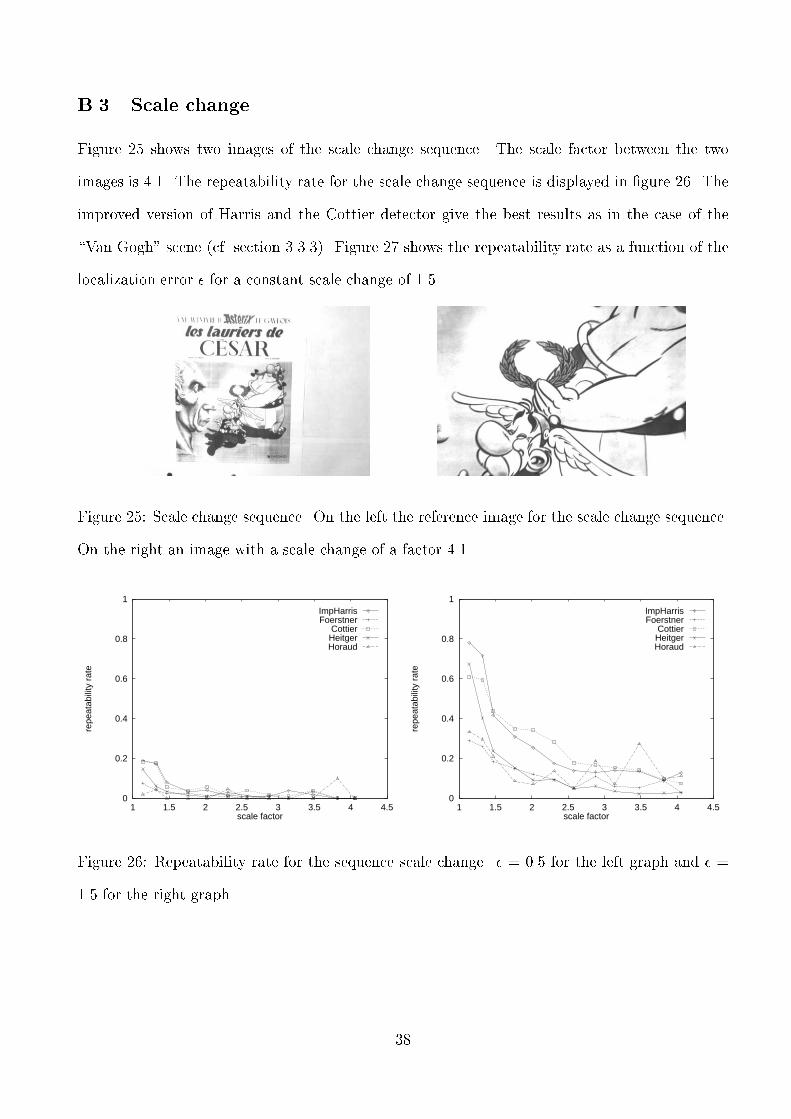
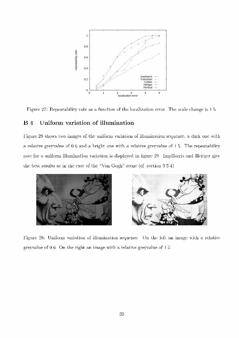
B.3 Scale changeFigure 25 shows two images of the scale change sequence. The scale factor between the twoimages is 4.1. The repeatability rate for the scale change sequence is displayed in �gure 26. Theimproved version of Harris and the Cottier detector give the best results as in the case of the\Van Gogh" scene (cf. section 3.3.3). Figure 27 shows the repeatability rate as a function of thelocalization error � for a constant scale change of 1.5.

Figure 25: Scale change sequence. On the left the reference image for the scale change sequence.On the right an image with a scale change of a factor 4.1.

0

0.2

0.4

0.6

0.8

1

1 1.5 2 2.5 3 3.5 4 4.5

repe

atab

ility

rat

e

scale factor

ImpHarrisFoerstner

CottierHeitgerHoraud

0

0.2

0.4

0.6

0.8

1

1 1.5 2 2.5 3 3.5 4 4.5

repe

atab

ility

rat

e

scale factor

ImpHarrisFoerstner

CottierHeitgerHoraud

Figure 26: Repeatability rate for the sequence scale change. � = 0.5 for the left graph and � =1.5 for the right graph.38

0

0.2

0.4

0.6

0.8

1

0 1 2 3 4 5

repe

atab

ility

rat

e

localization error

ImpHarrisFoerstner

CottierHeitgerHoraudFigure 27: Repeatability rate as a function of the localization error. The scale change is 1.5.B.4 Uniform variation of illuminationFigure 28 shows two images of the uniform variation of illumination sequence, a dark one witha relative greyvalue of 0.6 and a bright one with a relative greyvalue of 1.5. The repeatabilityrate for a uniform illumination variation is displayed in �gure 29. ImpHarris and Heitger givethe best results as in the case of the \Van Gogh" scene (cf. section 3.3.4).

Figure 28: Uniform variation of illumination sequence. On the left an image with a relativegreyvalue of 0.6. On the right an image with a relative greyvalue of 1.5.

39

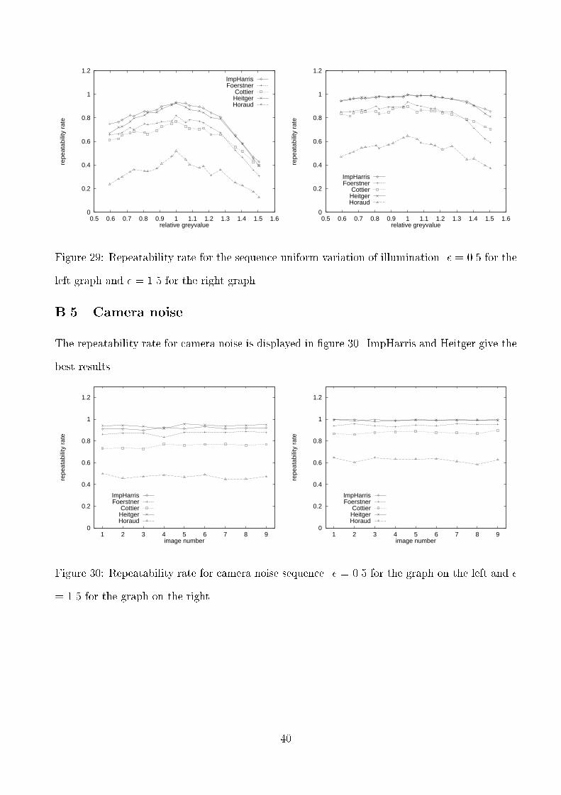
0

0.2

0.4

0.6

0.8

1

1.2

0.5 0.6 0.7 0.8 0.9 1 1.1 1.2 1.3 1.4 1.5 1.6

repe

atab

ility

rat

e

relative greyvalue

ImpHarrisFoerstner

CottierHeitgerHoraud

0

0.2

0.4

0.6

0.8

1

1.2

0.5 0.6 0.7 0.8 0.9 1 1.1 1.2 1.3 1.4 1.5 1.6

repe

atab

ility

rat

e

relative greyvalue

ImpHarrisFoerstner

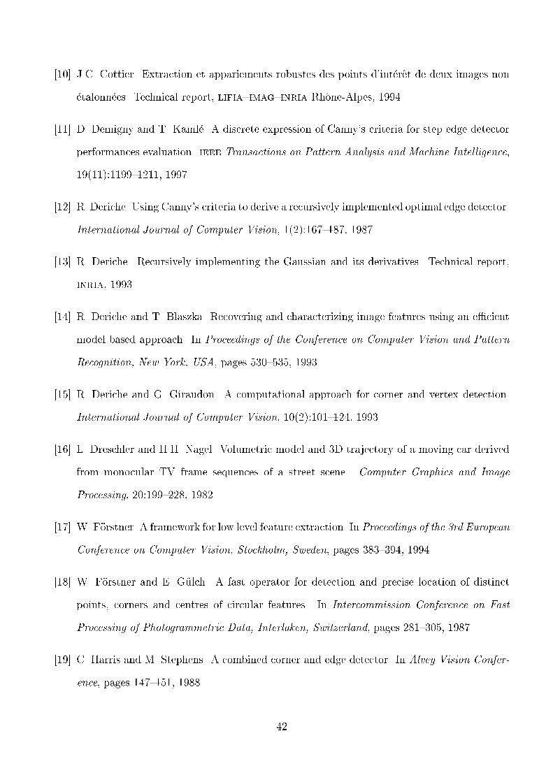
CottierHeitgerHoraudFigure 29: Repeatability rate for the sequence uniform variation of illumination. � = 0.5 for theleft graph and � = 1.5 for the right graph.B.5 Camera noiseThe repeatability rate for camera noise is displayed in �gure 30. ImpHarris and Heitger give thebest results.

0

0.2

0.4

0.6

0.8

1

1.2

1 2 3 4 5 6 7 8 9

repe

atab

ility

rat

e

image number

ImpHarrisFoerstner

CottierHeitgerHoraud

0

0.2

0.4

0.6

0.8

1

1.2

1 2 3 4 5 6 7 8 9

repe

atab

ility

rat

e

image number

ImpHarrisFoerstner

CottierHeitgerHoraudFigure 30: Repeatability rate for camera noise sequence. � = 0.5 for the graph on the left and �= 1.5 for the graph on the right.

40

References[1] H. Asada and M. Brady. The curvature primal sketch. ieee Transactions on PatternAnalysis and Machine Intelligence, 8(1):2{14, 1986.[2] S. Baker, S. Nayar, and H. Murase. Parametric feature detection. International Journal ofComputer Vision, 27(1):27{50, 1998.[3] S. Baker and S. K. Nayar. Global measures of coherence for edge detector evaluation. InProceedings of the Conference on Computer Vision and Pattern Recognition, Fort Collins,Colorado, USA, pages 373{379, 1999.[4] P.R. Beaudet. Rotationally invariant image operators. In Proceedings of the 4th InternationalJoint Conference on Pattern Recognition, Tokyo, pages 579{583, 1978.[5] K. Bowyer, C. Kranenburg, and S. Dougherty. Edge detector evaluation using empirical ROCcurves. In Proceedings of the Conference on Computer Vision and Pattern Recognition, FortCollins, Colorado, USA, pages 354{359, 1999.[6] P. Brand and R. Mohr. Accuracy in image measure. In S.F. El-Hakim, editor, Proceedings ofthe spie Conference on Videometrics III, Boston, Massachusetts, USA, volume 2350, pages218{228, 1994.[7] J. Canny. A computational approach to edge detection. ieee Transactions on PatternAnalysis and Machine Intelligence, 8(6):679{698, 1986.[8] C. Coelho, A. Heller, J.L. Mundy, D. Forsyth, and A. Zisserman. An experimental evaluationof projective invariants. In Proceeding of the darpa{esprit workshop on Applications ofInvariants in Computer Vision, Reykjavik, Iceland, pages 273{293, 1991.[9] J. Cooper, S. Venkatesh, and L. Kitchen. Early jump-out corner detectors. ieee Transactionson Pattern Analysis and Machine Intelligence, 15(8):823{833, 1993.41

[10] J.C. Cottier. Extraction et appariements robustes des points d'int�eret de deux images non�etalonn�ees. Technical report, lifia{imag{inria Rhone-Alpes, 1994.[11] D. Demigny and T. Kaml�e. A discrete expression of Canny's criteria for step edge detectorperformances evaluation. ieee Transactions on Pattern Analysis and Machine Intelligence,19(11):1199{1211, 1997.[12] R. Deriche. Using Canny's criteria to derive a recursively implemented optimal edge detector.International Journal of Computer Vision, 1(2):167{187, 1987.[13] R. Deriche. Recursively implementing the Gaussian and its derivatives. Technical report,inria, 1993.[14] R. Deriche and T. Blaszka. Recovering and characterizing image features using an e�cientmodel based approach. In Proceedings of the Conference on Computer Vision and PatternRecognition, New York, USA, pages 530{535, 1993.[15] R. Deriche and G. Giraudon. A computational approach for corner and vertex detection.International Journal of Computer Vision, 10(2):101{124, 1993.[16] L. Dreschler and H.H. Nagel. Volumetric model and 3D trajectory of a moving car derivedfrom monocular TV frame sequences of a street scene. Computer Graphics and ImageProcessing, 20:199{228, 1982.[17] W. F�orstner. A framework for low level feature extraction. In Proceedings of the 3rd EuropeanConference on Computer Vision, Stockholm, Sweden, pages 383{394, 1994.[18] W. F�orstner and E. G�ulch. A fast operator for detection and precise location of distinctpoints, corners and centres of circular features. In Intercommission Conference on FastProcessing of Photogrammetric Data, Interlaken, Switzerland, pages 281{305, 1987.[19] C. Harris and M. Stephens. A combined corner and edge detector. In Alvey Vision Confer-ence, pages 147{151, 1988. 42

[20] M. D. Heath, S. Sarkar, T. Sanocki, and K. W. Bowyer. A robust visual method for assess-ing the relative performance of edge-detection algorithms. ieee Transactions on PatternAnalysis and Machine Intelligence, 19(12):1338{1359, 1997.[21] F. Heitger, L. Rosenthaler, R. von der Heydt, E. Peterhans, and O. Kuebler. Simulation ofneural contour mechanism: from simple to end-stopped cells. Vision Research, 32(5):963{981, 1992.[22] A. Heyden and K. Rohr. Evaluation of corner extraction schemes using invariance meth-ods. In Proceedings of the 13th International Conference on Pattern Recognition, Vienna,Austria, volume I, pages 895{899, 1996.[23] R. Horaud, T. Skordas, and F. Veillon. Finding geometric and relational structures in animage. In Proceedings of the 1st European Conference on Computer Vision, Antibes, France,pages 374{384, 1990.[24] L. Kitchen and A. Rosenfeld. Gray-level corner detection. Pattern Recognition Letters,1:95{102, 1982.[25] J.J. Koenderink and A.J. van Doorn. Representation of local geometry in the visual system.Biological Cybernetics, 55:367{375, 1987.[26] R. Lagani�ere. Morphological corner detection. In Proceedings of the 6th International Con-ference on Computer Vision, Bombay, India, pages 280{285, 1998.[27] A. M. L�opez, F. Lumbreras, J. Serrat, and J. J. Villanueva. Evaluation of methods for ridgeand valley detection. ieee Transactions on Pattern Analysis and Machine Intelligence,21(4):327{335, 1999.[28] G. Medioni and Y. Yasumoto. Corner detection and curve representation using cubic B-splines. Computer Vision, Graphics and Image Processing, volume 39, pages 267{278, 1987.43

[29] F. Mokhtarian and A. Mackworth. Scale-based description and recognition of planar curvesand two-dimensional shapes. ieee Transactions on Pattern Analysis and Machine Intelli-gence, 8(1):34{43, 1986.[30] F. Mokhtarian and R. Suomela. Robust image corner detection through curvature scalespace. ieee Transactions on Pattern Analysis and Machine Intelligence, 20(12):1376{1381,1998.[31] H.P. Moravec. Towards automatic visual obstacle avoidance. In Proceedings of the 5thInternational Joint Conference on Arti�cial Intelligence, Cambridge, Massachusetts, USA,page 584, 1977.[32] H.H. Nagel. Displacement vectors derived from second order intensity variations in imagesequences. Computer Vision, Graphics and Image Processing, 21:85{117, 1983.[33] A. Papoulis. Probability, Random Variables, and Stochastic Processes. McGraw Hill, 1991.[34] L. Parida, D. Geiger, and R. Hummel. Junctions : Detection, classi�cation, and recon-struction. ieee Transactions on Pattern Analysis and Machine Intelligence, 20(7):687{698,1998.[35] P. Perona. Deformable kernels for early vision. ieee Transactions on Pattern Analysis andMachine Intelligence, 17(5):488{499, 1995.[36] P. J. Phillips and K. W. Bowyer. Introduction to the special section on empirical evalua-tion of computer vision algorithms. ieee Transactions on Pattern Analysis and MachineIntelligence, 21(4):289{290, 1999.[37] A. Pikaz and I. Dinstein. Using simple decomposition for smoothing and feature point detec-tion of noisy digital curves. ieee Transactions on Pattern Analysis and Machine Intelligence,16(8):808{813, 1994.[38] D. Reisfeld, H. Wolfson, and Y. Yeshurun. Context-free attentional operators : The gener-alized symmetry transform. International Journal of Computer Vision, 14:119{130, 1995.44

[39] K. Rohr. Recognizing corners by �tting parametric models. International Journal of Com-puter Vision, 9(3):213{230, 1992.[40] K. Rohr. Localization properties of direct corner detectors. Journal of Mathematical Imagingand Vision, 4(2):139{150, 1994.[41] B.M Romeny, L.M.J. Florack, A.H. Salden, and M.A. Viergever. Higher order di�erentialstructure of images. Image and Vision Computing, 12(6):317{325, 1994.[42] J.G. Semple and G.T. Kneebone. Algebraic Projective Geometry. Oxford Science Publica-tion, 1952.[43] J. Shi and C. Tomasi. Good features to track. In Proceedings of the Conference on ComputerVision and Pattern Recognition, Seattle, Washington, USA, pages 593{600, 1994.[44] E. Shilat, M. Werman, and Y. Gdalyahu. Ridge's corner detection and correspondence. InProceedings of the Conference on Computer Vision and Pattern Recognition, Puerto Rico,USA, pages 976{981, 1997.[45] M. C. Shin, D. Goldgof, and K. Bowyer. Comparison of edge detectors using an object recog-nition task. In Proceedings of the Conference on Computer Vision and Pattern Recognition,Fort Collins, Colorado, USA, pages 360{365, 1999.[46] M. C. Shin, D. Goldgof, and K. W. Bowyer. An objective comparison methodology of edgedetection algorithms using a structure from motion task. In Proceedings of the Conference onComputer Vision and Pattern Recognition, Santa Barbara, California, USA, pages 190{195,1998.[47] S. M. Smith and J. M. Brady. SUSAN - a new approach to low level image processing.International Journal of Computer Vision, 23(1):45{78, 1997.[48] C. Tomasi and T. Kanade. Detection and tracking of point features. Technical reportCMU-CS-91-132, Carnegie Mellon University, 1991.45

[49] Z. Zhang, R. Deriche, O. Faugeras, and Q.T. Luong. A robust technique for matchingtwo uncalibrated images through the recovery of the unknown epipolar geometry. Arti�cialIntelligence, 78:87{119, 1995.

46