evaluation of inverter reconnection for large solar...
TRANSCRIPT

Evaluation of Inverter Reconnection for Large Solar
Parks
Master of Science Thesis in the Master Degree Programme, Electric Power
Engineering
SELAM T. CHERNET
Department of Energy and Environment
Division of Electric Power Engineering
CHALMERS UNIVERSITY OF TECHNOLOGY
Göteborg, Sweden, 2010

Evaluation of Inverter Reconnection for Large Solar
Parks
SELAM T. CHERNET
Department of Energy and Environment
CHALMERS UNIVERSITY OF TECHNOLOGY
Göteborg, Sweden 2010

Evaluation of Inverter Reconnection for Large Solar Parks
© SELAM T. CHERNET, 2010
Department of Energy and Environment
Chalmers University of Technology
SE-412 96 Göteborg
Sweden
Telephone + 46 (0)31-772 1000
Mater thesis conducted at ABB Corporate Research (SECRC) in cooperation with
Chalmers University of technology
Chalmers Bibliotek, Reproservice
Göteborg, Sweden 2010


Acknowledgment
I would like to thank my supervisor Staffan Norrga, co supervisor Bengt Stridth in ABB Cooperate
research. My gratitude goes out to ABB Corporate research for giving a chance to work on such a
challenging project. I would like to thank my supervisor and examiner, Massimo Bongiorno, for his
valuable time and effort in helping challenge myself. Thank you for believing in me from the start and
enabling me to focus on my studies.
During my work, I also had the privilege to ask and enquire question, brain storm ideas with many
researchers who were quiet helpful in getting perspectives. My thanks go to George Demetriades, Enar
Salinas, Thomas Eriksson, Magnus öhrström, Marley Becerra, and all thesis co- workers who always kept
an open door to all my doubts and question.
Last but not least I would like to thank my family and friend who have enquired, threw in their helpful
tips, and taken a big load off my back. My heartfelt gratitude goes to my boyfriend Markos, you have
helped in so many ways than one (MLL), now is my turn to make it up to you. Above all, Praise to All
mighty God.

Abstract
The growing demand in energy consumption as a result of both accelerated growth in human population
and advancement in technology is exerting tremendous stress on our environment. Majority of electrical
production are typically provided from fossil fuels like coal, natural gases and oil which contribute highly
to the increasing CO2 production. To reduce the negative impact of these resources and reduce the
societies dependency on them, sustainable, renewable energy resources like biomass, geothermal, solar,
wind, ocean thermal, wave action and tidal action have come into focus. This master thesis looks into the
improvement of efficiency of large solar parks.
The work investigates the application of inverter reconnection mechanisms of solar inverters applied to
large solar park. This is performed by modeling the possible switching mechanisms in Mat lab and
analyzing the loss reduction potential of each inverter reconnection. The loss profile of solar inverter is
derived from datasheet values available for a 100KW and 500KW Gamesa Inverter. To generate the
output from the solar park, two types of commercial available photovoltaic simulation softwares were
used namely PVSyst 5.12 and INSEL 8.
To incorporate the effect of shading on the performance of solar park, the work also investigates
modeling of large solar parks. Three mathematical models were investigated and the results are presented.
The implementation of the model was done in Mat Lab. The modeling for large solar parks is performed
in order to investigate the performance of the inverter reconnection with respect to partial shading. Since
measurement setups weren’t available, none of the models can be verified with measured data. The model
results confirm theoretical analysis.

Table of Contents Acknowledgment
Abstract
1 Introduction .......................................................................................................................................... 1
1.1 Purpose ......................................................................................................................................... 1
1.2 Scope ............................................................................................................................................. 2
1.3 Definition ...................................................................................................................................... 2
1.4 Structure ....................................................................................................................................... 3
2 Problem Description ............................................................................................................................. 5
2.1 Inverter Reconnection .................................................................................................................. 5
2.2 PV Generator System Modeling .................................................................................................... 5
3 Literature Review .................................................................................................................................. 6
3.1 PV Generator System .................................................................................................................... 6
3.1.1 Generation Stage .................................................................................................................. 6
3.1.2 Inversion stage .................................................................................................................... 10
3.1.3 Efficiency issues .................................................................................................................. 18
3.2 Modeling of PV Generator System ............................................................................................. 21
3.2.1 Basic PV Cell modeling ........................................................................................................ 21
3.2.2 Simplified PV Generator Modeling ..................................................................................... 27
3.2.3 Cell based Modeling ............................................................................................................ 29
3.2.4 Module based Modeling ..................................................................................................... 31
3.2.5 Partial Shaded PV Generator Modeling .............................................................................. 34
4 Solution ............................................................................................................................................... 36
4.1 Inverter Reconnection ................................................................................................................ 36
4.2 PV generator modeling ............................................................................................................... 44
4.2.1 Module Based Modeling ..................................................................................................... 44
4.2.2 Simplified PV generator modeling ...................................................................................... 46
4.2.3 Partially shaded PV Generator Modeling ............................................................................ 47
5 Results ................................................................................................................................................. 50
5.1 Loss calculation for different Inverter Reconnection Scheme .................................................... 50
Result for inverter reconnection Scheme 1 ......................................................................................... 51

Result for inverter reconnection Scheme 2: ....................................................................................... 52
Result for inverter reconnection Scheme 3: ....................................................................................... 53
Result for inverter reconnection Scheme 4: ....................................................................................... 55
5.2 Test on General Model ............................................................................................................... 59
5.3 Simplified PV Generator Modeling for Inverter reconnection Analysis...................................... 64
5.4 Partially Shaded PV Generator Modeling ................................................................................... 70
5.5 Module Based Modeling ............................................................................................................. 79
6 Conclusion ........................................................................................................................................... 82
7 Reference ............................................................................................................................................ 83
Appendix A: Research on Cloud Effects on PV Generator system .......................................................... 85


1
1 Introduction This chapter presents a short description of the thesis work. Sections one describes the purpose of the
work. Section two includes the post condition as well as the limitation and scope of the work. The area
investigated, results and short comings of the work are also presented in this section. Section 3 of this
chapter presents definition of terms used throughout the report. The last section gives a description of
report’s structure.
1.1 Purpose To address the environmental impact of today’s power production methods and the increasing energy
consumption, a lot of research is carried out to increase the large scale applicability of sustainable power
production systems like wind and solar. Today large photovoltaic (PV) generation system with a capacity
up to 60 MW exists [23]. With a price of range of 3-5cents/Kwh, the price of energy from PV generator is
much more expensive compared to conventional power generation. Despite the cost, due to attractive
incentives presented by government, PV generation systems are expanding quiet rapidly. To bring the
cost down would require several coordinated initiatives like improvement on efficiency of components
building up the system. At the same time the improvement of the system efficiency to bring the cost down
is regarded as a solution.
Different stage exists before the power generated by the PV array reaches the medium voltage grid.
Figure 1.1 below presents the various stages and their associated losses.
Figure 1.1 Schematic view of a PV generation system
The loss characteristic of PV inverter doesn’t present a linear relation to the power. This is associated to
constant iron loss that exists in the low voltage transformer. To alleviate the efficiency problem associated
with PV inverters, inverter manufacturers employee different inverter reconnection strategies to operate
two or more inverters as a single unit. The applicability of these strategies on large PV generator system
will be covered in this work.
The output of a PV generator system can be simulated using different commercially available software
namely PVSyst, INSEL, PV*SOL, PV design pro. But to this day, how this software treat the effect of
partial shading on the output behavior of large solar parks isn’t really clear. Plus most function that are
available with some software deal with shading caused by stationary objects in the vicinity of PV
2
generator [7]. To develop a model that can consider the effect of partial shading can be quiet a valuable
tool.
1.2 Scope
The scope of the report covers four inverter reconnection methods. These methods are analyzed with
respect to their loss reduction potential. The whole work is primarily aimed at grid connected PV
generator system. When it comes to the modeling, three PV generator modeling approached where chosen
and tried. The reader at this point should be warned that, the results from the modeling are not compared
to any experimental data. In addition the models employed do not cover partial shading scenario caused
by fast moving cloud. The work can be taught of a starting ground to modeling the effect of shading on
large PV generator system.
1.3 Definition
algorithm Method of solving a problem using a sequence of finite instruction
Equivalent
circuit
Simplest form of a circuit that preserves all electrical characteristics of a
more complex system
Flow chart Diagram that represents an algorithm of a process. A schematic
representation of how the different stage in a process are interconnected
Galvanic
isolation
Principle of separating functional section of electrical system so that no
current flows directly between separated sections
Grid System of electrical distribution serving a large area that is maintained by
electrical utility
irradiation Amount of solar energy received on a surface in a certain amount of time
MPPT Maximum power point tracker, a power conditioning unit that operated a PV
generator at its maximum power point
model A set of mathematical equation describing the behavior of a system
modeling All process involved to express mathematical the behavior of a system
nonlinear A direct relationship doesn’t exist between the input and output
Photon Basic unit of light
Photovoltage Voltage generated across an unloaded photovoltaic generator at a particular
temperature and irradiance as measured with a voltmeter

3
1.4 Structure
The structure of the report is as follows
Chapter 1: Introduction describes the purpose of the report, the scope of the work and terms and
abbreviation used.
Chapter 2: Description of the problem to be solved
Chapter 3: Literature review on PV generator system, reconnection methods to improve efficiency of the
system and different possible approach to model a large PV generator system
Chapter 4: Discussion on the approach taken in solving the problem in section 2. It starts by presenting
the methods for inverter reconnection. It then covers the implemented method for PV generator modeling
Chapter 5: Result shows all the result in the methods implemented. A small description and discussion for
some results are presented along.
Chapter 6: Conclusion and future work

4

5
2 Problem Description
2.1 Inverter Reconnection
In large Photovoltaic generator system, several inverters are operated in parallel to convert the DC power
generated by the system. The output from this inverter can be connected to a medium voltage transformer
that is connected to medium voltage transmission line. Present day PV generators donot have loss
characteristics that vary linearly with load. Constant power losses exist due to iron losses in low voltage
transformer. Transformer less PV inverters are available that can reduce this problem but due to grid
requirement for galvanic isolation between PV generator system and the grid, their universal applicability
are limited.
In order to mitigate the problem at hand, several solutions have been proposed where the number of
inverters operated is reduced during low load condition. This helps in avoiding operating inverters in their
low efficiency region. It would be interesting to evaluate the different solution with respect of loss
reduction potential.
2.2 PV Generator System Modeling
Shading upon a PV generation system can bring down the performance of the generation system. To this
day several PV Generator system simulation program exist that can be used to simulate the output of PV
generator system. Some not all developed program have features to treat shading condition caused by
stationary objects. In addition how this software deal with condition of partial shading is not clearly
defined. A model that can be used to generate the output of a non uniformly illuminated PV generator
system can be a good asset.

6
3 Literature Review
3.1 PV Generator System Photovoltaic generation system is becoming quiet significant among sustainable energy system since it
offers many advantages such as no fuel cost, no pollution, requirement of little maintains and no noise.
On the down side PV module until today has relatively low conversion efficiency in the order of 12-15%
[24]. In medium and large size PV power system, the efficiency of the system becomes a key design
issue. Various conversion stages exist to convert the energy from the sun to a usable energy form. The
basic units in the conversion stage will be discussed. A simplified block diagram representing the process
is shown below.
Generation
stageInversion stage Voltage Adaptation
Solar
energyDC AC AC
AC Grid
Figure 3.1 Simplified block diagram of a PV generator system
3.1.1 Generation Stage
PV Cell and PV module
PV cells are large area semiconductor devices. In simple words, a PV cell can be explained as a two
terminal device that conducts like a diode in the dark and produce photo voltage when illuminated by
light. An ideal PV cell can be represented as an ideal current source in parallel with a diode (fig 3.2). The
current source represents the current generated by the PV cells as a result of Photons received and is
dependent on the amount of irradiation (will be proved shortly) and temperature whereas in the absence of
light the PV cell behaves as a diode.
DiodeIph
VpvID
Iph Ipv
Figure 3.2 Equivalent circuit of an ideal PV cell.
The current from an ideal PV cell ( ) can be expressed interms of the photon current ( ) and the diode
current ( )
3.1.

7
The diode current can be expressed using the Shocktey’s diode equation as
3.2.
Where Io = Reverse saturation current of the diode
Vd = Voltage across diode
K= Boltzman’s constant
q = Electron Charge
T = Junction Temperature [K]
The I-V characteristics equation for an ideal PV cell can be obtained by inserting equation 3.2 into 3.1
3.3.
Under short circuit condition, i.e. when = 0 in equation 3.3, the cell’s current is equivalent to the
photon generated current. This shows, the cell’s current to be directly proportional to the cell’s irradiance.
On the other hand, the effect of irradiation on the open circuit voltage is solved by setting ( = 0) in
equation 3.3.
3.4.
From equation 3.4, it can be observed that the open circuit voltage is only logarithmically dependent on
the cell illumination where as it is directly proportional to the operating temperature.
Since in reality no solar cell is ideal, a shunt resistance (to represent the leakage current through solar
cell) and a series resistance (representing resistance in emitter and base region) are added to the model.
The equivalent circuit representing a PV cell using the one diode model is shown below. The detailed
derivation of the model will be covered in part 3.2.1

8
Diode Rp
Rs
Iph
Vpv=Voc
Ipv=0
ID
Iph
Ip
Figure 3.3 Equivalent circuit of a non ideal PV cell
In Equation 3.4, it is shown that the voltage current characteristic of any photovoltaic unit is dependent on
the solar radiation and working temperature. When charged by a light source, a PV cell generates a DC
voltage of 0.5-1 volts and in short circuit, a photon current density of some ten’s of milliamps/cm2 [14].
The voltage level from a single PV cell is too small for any application, and as a result several cells are
connected in series and encapsulated to form modules. For standalone system 36 cell modules is the
normal standard. But recently due increasing grid connected PV generator system, the power requirement
of each module has gone up. In most commercial available module it is now usual to have 54 cells or 72
cells in series [24]. The most used parameter for characterizing a PV module is the open circuit voltage
and the short circuit current which are generally provided on the manufacturer’s data sheet. The use of
these parameters will be discussed in later sections.
The characteristic I-V curve of a module is highly nonlinear [2]. During short circuit condition, the
maximum current from the PV module is attained. If we attach a load resistance and increase it, the
current starts to fall off at a lower rate until a knee point. Beyond the knee point the current falls
drastically to zero (where V=Voc). Figure 3.4 illustrates this and the effect of irradiation and temperature
on the I-V characteristic of a PV module.
(a)

9
(b)
Figure 3.4 I-V characteristics of a Photovoltaic module (a) different irradiation condition (b) different operating temperature.
The power (P) versus voltage (V) can be found by direct multiplication of the current (I) and the voltage
(V) for each operating point. The P-V characteristic for increasing irradiation condition (figure 3.5 a) and
decreasing temperature (figure 3.5 b) is shown. Important point we need to observe from figure 3.5 is
that, there exists a single point where the power output of the PV module is maximum. This point is
referred to the maximum power point (MPP).
(a)
Increasing
temperature

10
(b)
Figure 3.5 P-V characteristics of a Photovoltaic module (a) different irradiation condition (b) different operating temperature.
Since cells are series connected in a module, it is important that the I-V characteristics of the cells match
as close as possible. Shading of a single or string of cells in a module would cause the output current of
the shaded portion to be lower. The series connection forces all cells to operate at the same current. If the
string current goes beyond the short circuit current capacity of the shaded cell, the cells starts to produce
negative voltage (instead of a source it starts to act as a sink). The power produced by the unshaded cell is
dissipated by the shaded cell. As a result a heating phenomena known as hotspot occurs [12]. If the
summation of voltage of the unshaded cell exceeds the diode reverse breakdown voltage, an irreversible
damage occurs on the cell.
PV Generator
To achieve a higher level of voltage, modules are connected in series to form strings and to achieve a
higher level of current; the strings are connected in parallel. For grid connected system it is nowadays
common to have the output voltage value of the PV generator greater than the grid voltage value [4].
These increase the overall efficiency of the system by avoiding a boost process within the conversion
stage. On the other hand, the PV generator total efficiency would be compromised due to mismatch loss
as the number of module connected in series increases [14]. Therefore during the design process an
optimal solution should be reached taking into consideration the customer’s choice on Inverter type.
3.1.2 Inversion stage
Since the generated power is in DC, the output from the system is then feed to the grid after passing
through an inversion stage. The inversion stage consists of a DC-DC stage using power electronics: for
adaptation of load characteristics with that of the PV generator (A maximum power point tracker) and a
second stage which is an inverter in order to perform the DC-AC conversion

11
MPP Point and MPP Tracker
The output power of PV generator is the product of the current delivered and the operating voltage of the
generator. In a PV generator, there exists a single point where the value of the current and the voltage
results in a maximum power. The mathematical equation describing the current voltage relation has an
exponential behavior which shows that there a knee beyond which the product of the current and voltage
fall drastically. This can be seen in figure 3.5 of the previous section. Moreover the characteristics curve
varies with varying irradiation and temperature condition. Hence where we operate is highly
determination for the output from our generator.
If direct coupling between the PV generator and the system load, a problem lies in the mismatch between
the operating point of the system load and the PV generator’s maximum power point. This can be
explained using figure 3.6. Assume that the characteristics I-V curve of the system load line is as shown
by the straight line. The I-V curve for the PV generator which varies with the varying irradiation level is
shown. When the load is directly connected to the PV generator, the overall system operating point is the
intersection point of the two curves, which is further away from the actual MPP point of the PV generator.
To operate the PV generation at its most efficient point, maximum power point trackers (MPPT) are
employed.
IPV
Load line 1
Load line 2
Maximum
Power point
Cu
rre
nt (A
)
Voltage (V)VPV
Increasing
irradiance
Figure 3.6 I-V curve of PV Generator and load I-V characteristics
According to the definition stated in Wikipedia, a MPPT is a high efficiency DC-DC converter used to
present an optimum electrical load to PV generator so that it operates at its MPP point while at the same
time produce a suitable voltage for the load. The choice whether the converter should be a buck or a boost
or a buck boost depends on the requirement of the load voltage. Many algorithms exist for
implementation of MPPT. The algorithms are used to determine the required duty cycle for the DC-DC
converter. To get an overview of how they function, two common algorithms are discussed here
The most common algorithm is “perturb and observe” (P&O) algorithm. In this algorithm Voltage is
incremented in steps by a fixed amount and the change in power (dP/dv) is observed. The algorithms then
only changes direction when it detects a drop in power in between the steps. Figure 3.7 is used to describe
the algorithm

12
Measure Voltage[V(i)] and Current[I(i)]
Calculate Power
P(i)= V(i)*I(i)
Is
P(i)>P(i-1)
Is V(i)>V(i-1)Is V(i)>V(i-1)
Vref(i)=Vref(i) - CVref(i)=Vref(i) + CVref(i)=Vref(i) + C Vref(i)=Vref(i) - C
No
YesNo
NOYes
Yes
Return
Figure 3.7 Flow chart showing “perturb and observe” algorithm.
The converter by adjusting its duty cycle puts up Vref for the PV generator and measures the change in
power and the cycle continues. This algorithm is the most common used because of its simplicity. The
downside to this algorithm is that it would have oscillation around the MPP point [2]. Another major fault
with P&O algorithm is its faulty performance under fast irradiation changes (caused by a cloud) [10]. The
algorithm increments the voltage and measures the change in power ( P), if the power increases, in the
next cycle the voltage is increased. Here the increase in power can be as a result of increased irradiation
level as a result of a cloud moving away from the PV generator. This causes the voltage to be incremented
where as the MPP for the present operating condition is at a lower voltage. This causes the search for
MPP point to deviate from the actual MPP point.
An algorithm that is proposed to overcome the fault of the P&O algorithm is the Incremental
conductance algorithm. At MPP the derivation of the power with respect to voltage equals zero.
3.5.

13
3.6.
By rearranging equation 3.6 the conductance can be expressed
3.7.
The Algorithm using a flowchart is presented below
Measure V(i) and I(i)
dI = In - I(i)
dV = Vn - V(i)
Is
dV = 0?
Is
dI/dV = -I/V ?
Is
dI = 0?
Is
dI/dV > -I/V ?
Vref=Vref + C Vref=Vref + CVref=Vref - CVref=Vref - C
Is
dI >0?
Vn=V(i)
In=I(i)
yes
yesyes
yes
No
No No
No
Noyes
Figure 3.8 flow chart showing incremental conductance algorithm
Where In and Vn are stored value at the end of the preceding cycle. The Vref is used by the DC-DC
convertor to adjust the operating point of the generator. In this algorithm the change in the atmospheric
condition (that is a change in the irradiation level) can be detected using the stage dI≠0.

14
Inverter Configurations
PV inverters, whose function is to converter DC into AC in addition, are responsible to extract maximum
energy out of the PV generator. For this purpose most inverters have built in mechanism for maximum
power point tracking.
Due to demands set by the different standard that has existed till present day, PV inverter technologies
have evolved in various dimensions. Most references categorize them based on three major criteria:
1. Conversion stage involved
2. Galvanic isolation - Transformer and Transformer less
3. Power decoupling
1. Conversion stage involved A single power conversion stage: In this topology, the task of MPP tracking, possible voltage boost (if
necessary) and DC to AC conversion is all performed by one unit. This configuration is really common in
most commercially available central inverters.
Dual power conversion stage: this involves a separate DC-DC conversion stage for MPP tracking and
possible voltage boost and a DC-AC conversion stage for grid adaptation.
Dual Power conversion stage with numerous DC-DC stages: This involves individual DC-DC conversion
where each string is equipped with individual MPP tracking with possible voltage boost that feeds to a
common DC port. A single DC-AC inverter is responsible for grid adaptation.
(a) (b) (c)
Figure 3.9 Inverter configuration (a) single conversion stage (b) double conversion stage with a single DC - DC stage (c) dual conversion stage with multiple DC-DC conversion stage
2. Galvanic isolation - Transformer and Transformer less A stray capacitance exists between the PV module and the ground [26]. In large PV generator, the stray
capacitance can be really significant causing severe oscillation with the stray inductance of the circuit [3].
To avoid this situation a galvanic isolation is required in the conversion stage. Some topologies involve a
line frequency transformer that is placed between the grid and the inverter. Since it involves line
frequency transformer, the size weight and cost associated is seen as a major disadvantage. Others
topology involve a high frequency transformer that is embedded in the DC-DC converter which serves as

15
the MPP tracker. Although we get the advantage of smaller size and weight of using a high frequency
transformer, the losses increase as a result of increased number of power processing stage. It should be
pointed out that the existence of a transformer electrical decouples the PV generator from the grid.
There also exists transformer less configuration. This configuration has the advantage of lower losses,
lighter weight and higher efficiency. This configuration in a single phase inverter is grounded on the AC
side. This is due to the neutral of the grid been connected to earth somewhere. Grounding on the DC side
can also occur due to two reasons. One is system grounding of the negative or the positive terminal of the
module. The other is, in an ungrounded PV generator, stray capacitance that exists between the module
surface and the ground creates a closed path for an undesired high frequency current. To avoid such
problem different topologies that solidly ground the DC link is discussed in ref 4. There also exists the
issue of safety standards in some countries that require galvanic isolation [4] between the grid and the PV
generator.
3. Power Decoupling It is the requirement in most grid code that the power that is feed to grid has a power factor of one. This
requires a current that is inphase with the voltage. Therefore the power injected to the grid can then be
written as
3.1.
It can be observed from above that the power on the AC side pulse at twice the grid frequency. If we
assume the conversion stage as lossless, Pac=Pdc, this pulsation is observed as a ripple on the dc side
voltage. As a result all single phase inverter are equipped with a DC link capacitor so as to suppress the
ripple in the voltage. The existence of this electrolyte capacitor decreases the inverters lifetime [3]. This is
not a problem in case of 3 phase inverters since they feed power to the grid in a continuous manner [25].
PV Generator configuration
When it comes to medium and large size PV generator system, where several strings are connected to
achieve higher power, the choice of plant design becomes important. Different PV generator
configuration exist which are generally classified as
1. Central configuration 2. String configuration 3. Multi-string configuration 4. Modular configuration
1. Central configuration
Depending on the voltage requirement several PV modules are connected in series to form a string.
Several strings then are connected in parallel to achieve a certain power level. In this configuration each

16
string feeds its out to a single DC bar. A central inverter capable of covering the whole range of input
power of the PV generator is connected to the DC bar. This is illustrated in the figure below.
DC barAC grid
Figure 3.10 Central Configuration
In this system, a single MPPT that is incorporated within the inverter does the maximum power point
tracking. The DC-AC conversion efficiency of PV inverters is very low in the low power range as a result
of constant iron loss in the transformer. The efficiency of the system therefore falls drastically when the
input from the PV generator falls low. This is one of the main demerits of this configuration.
Another disadvantage of the central inverter configuration is as a result of different operating condition
(temperature and irradiation) along each string, especially in larger solar parks, the voltage associated
with the maximum power point of each string doesn’t necessarily coincide with the operating voltage at
the DC bar. As a result we don’t get to harness the maximum energy out of the PV generator. In addition,
the requirement of a high voltage DC cable between the PV generator and the inverter and the reliability
of the whole system on a single inverter is also some of the stated disadvantage of this configuration
2. String Configuration In this configuration PV string, made of series connected PV modules are connected to individual
inverter. The output from each inverter is then feed to a common AC bar. This is illustrated in figure 3.11.
The advantage of this system is that the inverter equipped with an MPPT is able to extract the max energy
out of each string. For large system this configuration would be really expensive as a result of increased
number of string equipped with inverters. This configuration has more advantage for small installation
where each string has different orientation, like installation on roof tops. In large installation where the
shading and different orientation of PV modules has been avoided in the design stage, this configuration
is not the best choice due to the associated higher price per KWh [6].

17
AC Grid
Figure 3.11 String configuration
3. Multistring configuration
This configuration is an intermediate between the string configuration and the central configuration. Here
several strings are connected in parallel feeds into a DC box. A single inverter connected to the DC box
performs the AC-DC conversion. Large commercial available PV inverters have Multiple MPPT as a
feature. If such large inverters are employed, the output from the aggregated strings can be feed to
individual DC input of the inverter. The advantage of this system as compared to the central inverter
topology is the amount of reduced string operated under a single MPPT.
DC box
DC box
AC grid Figure 3.12 Multistring configuration
18
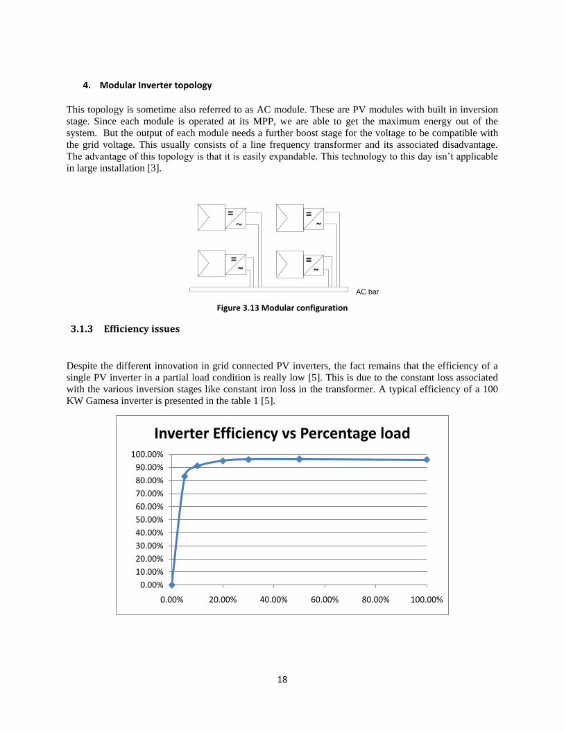
4. Modular Inverter topology
This topology is sometime also referred to as AC module. These are PV modules with built in inversion
stage. Since each module is operated at its MPP, we are able to get the maximum energy out of the
system. But the output of each module needs a further boost stage for the voltage to be compatible with
the grid voltage. This usually consists of a line frequency transformer and its associated disadvantage.
The advantage of this topology is that it is easily expandable. This technology to this day isn’t applicable
in large installation [3].
=~ ~
~~
=
==
AC bar
Figure 3.13 Modular configuration
3.1.3 Efficiency issues
Despite the different innovation in grid connected PV inverters, the fact remains that the efficiency of a
single PV inverter in a partial load condition is really low [5]. This is due to the constant loss associated
with the various inversion stages like constant iron loss in the transformer. A typical efficiency of a 100
KW Gamesa inverter is presented in the table 1 [5].
0.00%
10.00%
20.00%
30.00%
40.00%
50.00%
60.00%
70.00%
80.00%
90.00%
100.00%
0.00% 20.00% 40.00% 60.00% 80.00% 100.00%
Inverter Efficiency vs Percentage load

19
Load (%) Efficiency (%)
5 83.30
10 91.21
20 95.04
30 96.06
50 96.41
100 96.00
Table 1 Efficiency as a function of nominal power for a 100KW Gamesa PV inverter
The low efficiency of the inverters during partial load has become a bottle neck. To avoid the operation of
the inverters in their low efficiency region, different solution where proposed where the number of
inverters serving a PV generator system were reduced during reduced output from the PV generator. Two
concepts stand out, the master slave concept and the team concept.
Master – slave concept
Instead of having a single large inverter, several smaller inverters are operated in the master slave mode.
When the PV generator starts to produce enough power, the master inverter switches on and takes over
operation. As the produced power exceeds a certain threshold, the second inverter (1st slave) is switched
in and for further increase of power the third inverter is switched. With increase in production more
inverters are switched in so as all inverters are operated at their optimum efficiency level. When PV
generator power output decreases due to significant variation in irradiation, the slave units are
automatically disconnected. The advantage with this concept is avoiding operating inverters in their low
efficiency regions.
ACDC
PV Generator
DC
contactors
DC
contactors
DC
contactors
DC bar
AC GridDC
DC
AC
AC
Figure 3.14 Single line diagram Master slave operation of inverters
Another stated advantage using this concept is the rotating master. When the PV generator system starts
to operate the next day, the master inverter is freely chosen from among the slave inverters. This helps to
evenly distribute the master inverter operating time among all inverters. If a master inverter fails any

20
inverter among the slaves can resume its task. The obvious drawback with this operation is it fails to
utilize the maximum power point tracking capabilities of each inverter.
3.1.3.1 Team Concept
In some references this is put as the concept that brings string concept with that of master slave concept
together. The PV generator is divided into parts. Each part feed its output to individual DC box. A DC
switch exists for disconnecting the PV part during maintenance. When output power is high each part is
connected to dedicated inverter and the park operates in a multi-string mode. When output is reduced,
inverters can be disconnected and output from the parts can be rerouted to fewer inverters. The advantage
with this operation is at high output, the maximum power tracking capabilities of each inverter is utilized.
But on the other hand this concept requires additional hardware for routing during low output condition.
ACDC
DC box
DC box
DC box
DC
contactors
DC
contactors
DC
contactors
DC
Switches
DC
Switches
DC
Switches
AC Grid
DC
DC
AC
AC
ACDC
DC box
DC box
DC box
DC
contactors
DC
contactors
DC
contactors
DC
Switches
DC
Switches
DC
Switches
DC
DC
AC
AC
DC
contactors
DC
contactors
DC
contactors
DC
contactors
Figure 3.15 Single line diagram team operation of inverters

21
3.2 Modeling of PV Generator System
3.2.1 Basic PV Cell modeling
In the course of time various equivalent circuit model of a PV cell has been developed. The one diode
model which is the most commonly used equivalent circuit for PV cell modeling will be discussed in this
part. A small introduction in part 3.1.1 described the working of an ideal PV cell and the equivalent
circuit of PV cell was discussed. A detailed derivation is presented in this section. Figure 3.16 is a
repeated here for the convinces of the reader.
Diode Rp
Rs
IphVpv
Ipv
ID
Iph
Ip
Figure 3.16 Equivalent circuit of a one diode model of a single PV cell
According to basic circuit equation, the cell current, Ipv can be described by equation 3.8
3.8.
Using the basic equation for a diode, the diode current as a function of the diode voltage can be expressed
as
3.9.
A term known as the thermal voltage is used to simplify equation 3.10
Where
3.10.
The diode voltage, VD in equation 3.9 and 3.10 can be easily derived from the equivalent equation as a
function of PV cell’s voltage and current as below

22
3.11.
Inserting equation 3.11 into equation 3.10
3.12.
The current through the parallel resistance (Ip), can be expressed in terms of the diode voltage and the
parallel resistance
3.13.
Putting together equation 3.13, 3.12 and 3.8, we arrive at equation 3.14
(a) 3.14.
Equation 3.14 describes the current voltage characteristics of a PV cell using the one diode model
representation. The above equation has five unknown values namely, Rs, Rp, Iph, Io and Ao which need to
be determined before equation 3.14(a) can be used. To determine these values, a set of 5 equations is
needed. Since none of these values are provided on the manufacturer’s datasheet, some mechanism needs
to be developed to determine this value for cell level. What we can get out of the manufacturer’s data
sheet is the total module short circuit current, module open circuit voltage and the module current and
voltage value at the maximum power point. Equation 3.14(a) is then upgraded to a module level by
adding a term Ns that represents the number of series connected cell in the module (refer to equation
3.14(b)). Provided that we know the short circuit current, open circuit voltage and maximum power point
current and voltage value for the module, we can define 3 conditions for the equivalent circuit shown in
fig 3.16. These conditions are discussed below. Later after solving the value of Rs, Rp, Iph, Io and Ao for
the module, the cell values for Io, Iph and Ao would be the same as that for the module where as the Rs
and Rp value equals the Rs and Rp value of the module divided by the no of cells in series.
(b) 3.14.

23
Condition 1: short circuit condition
Diode Rp
Rs
Iph
Vpv=0
Ipv=Isc
ID
Iph
Ip
Figure 3.17 equivalent circuit of PV cell using one diode model under short circuit condition
Neglecting the diode current which is assumed to be really small compared to the Isc, the photon current
Iph, can be expressed as the sum of the short circuit current and the current through the parallel resistance
as below
3.15.
During short circuit condition, Vpv=0; equation 3.14(b) is then reduced to equation 3.16
3.16.
Condition 2: Open circuit condition
Diode Rp
Rs
Iph
Vpv=Voc
Ipv=0
ID
Iph
Ip
Figure 3.18 Equivalent Circuit of PV cell using one diode model under open circuit condition
Under open circuit condition the PV cell current, Ipv=0 and Vpv=Voc. Applying this in equation 3.14(b),
we arrive at equation 3.17
3.17.
Condition 3: Maximum Power Point condition
At the maximum power point Ipv=Impp and Vpv=Vmpp. Inserting this conditions in equation 3.14(b), we get
equation 3.18

24
3.18.
The derivative of power with respect to voltage at the maximum power point is zero.
mppmpp IIVVdV
dp
,
3.19.
it can be observed from figure 3.17 that during short circuit condition the change in current with respect
to voltage is mainly determined by the shunt resistance [11]. At short circuit condition, this can be
expressed as
sII RdV
dI
sc
1
3.20.
Taking equation 3.17 and solving for the photon current, we arrive at equation 3.21
3.21.
By substituting equation 3.21 into equation 3.16, a new equation for the short circuit current is derived
3.22.
Since the term
is really small compared to the other term in the same bracket, this term is
neglected [11] and we arrive at equation 3.23
3.23.
Solving equation 3.23 for Io
3.24.

25
Taking equation 3.21 and 3.24 and inserting it into equation 3.18, we get
3.25.
Now considering the derivative of the power with respect to voltage at MPP
VdV
dII
dV
IVd
dV
dp
mppmpp IIVV
*)(
,
3.26.
The second term in equation 3.26 requires that the derivative of equation 3.25 with respect to voltage. But
the equation of Impp needs numerical methods. As a simplification let us express equation 3.25 in the form
below
3.27.
where equation 3.27 represents the right side of equation 3.25. Differentiating equation 3.27
3.28.
3.29.
F
DVI
dV
dpmppmpp
II mpp
1
. 3.30.
Where D=ppts
ts
ocsmppmpp
sscocpsc
RRVN
VN
VRIVRIVRI
1
**
)*
*exp()**(
26
F=p
s
pts
ts
ocsmppmpp
sscocpsc
R
R
RVN
VN
VRIVRIVRI
**
)*
*exp()*( *
Taking equation 3.20 and 3.28
p
s
p
IIs
R
RH
RH
Rsc
1
1
1 3.31.
Where H=pts
ts
ocsscsscocpsc
RVN
VN
VRIRIVRI
**
)*
*exp()**(
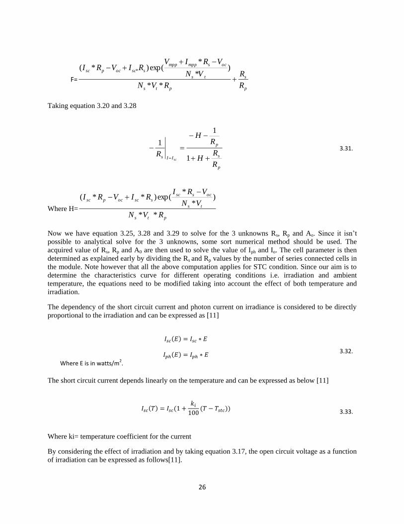
Now we have equation 3.25, 3.28 and 3.29 to solve for the 3 unknowns Rs, Rp and Ao. Since it isn’t
possible to analytical solve for the 3 unknowns, some sort numerical method should be used. The
acquired value of Rs, Rp and A0 are then used to solve the value of Iph and Io. The cell parameter is then
determined as explained early by dividing the Rs and Rp values by the number of series connected cells in
the module. Note however that all the above computation applies for STC condition. Since our aim is to
determine the characteristics curve for different operating conditions i.e. irradiation and ambient
temperature, the equations need to be modified taking into account the effect of both temperature and
irradiation.
The dependency of the short circuit current and photon current on irradiance is considered to be directly
proportional to the irradiation and can be expressed as [11]
Where E is in watts/m2.
3.32.
The short circuit current depends linearly on the temperature and can be expressed as below [11]
3.33.
Where ki= temperature coefficient for the current
By considering the effect of irradiation and by taking equation 3.17, the open circuit voltage as a function
of irradiation can be expressed as follows[11].

27
3.34.
Equation 3.33 needs numerical methods to solve Voc(E). The open circuit voltage shows a linear
dependency with temperature [11] and can be expressed as
3.35.
The dependency of saturation current on temperature Io(T) is derived by substituting the terms of equation
3.24 to include the temperature effect.
3.36.
In a similar fashion, transforming the terms of equation 3.21 to include temperature effect, the photon
current dependency on temperature can be represented as below
3.37.
The current voltage characteristics can be expressed by inserting equation 3.33, 3.34, 3.35, 3.36, 3.37 into
equation 3.14. The effect of temperature on value of series and parallel resistance is not accounted for in
this modeling.
3.2.2 Simplified PV Generator Modeling
As the name indicates it is a simplified model as it assumes all modules connected in series to
form a string are subjected to the same operating condition. The model also ignores any phenomena that
occur in the cells making up each module.
Before proceeding let us say a few things about blocking diode and bypass diodes. In a PV
generator system where several strings are connected in parallel, voltage variation among parallel strings
causes the current produces by one string to be sunk by an adjacent string of a lower potential. To avoid
back flow of current among adjacent strings, each string is equipped with a blocking diode in series. On a
cell level; partial shadowing will have the same effect as receiving a reduced illumination [8]. Since in
this model we assume that all the cells are operated under the same condition, it is fair to assume that
partial shading will have the same effect as reduced illumination on the PV module. The current output of
the shadowed module which is proportional to the illumination is thus reduced. Since all modules are
connected in series, a situation occurs where the current from the unshaded modules which is greater than
the short circuit current of the shaded module flows in the string. This causes the shaded module to
operate in the 2nd quadrant and the module acts as a sink instead of a sources. To mitigate the problem
bypass diode are connected anti parallel with the module. With bypass diode, when the current exceeds
the short circuit current the diode is forward biased and all the current greater than the shaded module
short circuit current is bypassed through the diode. The string output voltage is reduced by the amount
equivalent to the bypassed module output voltage plus forward voltage drop of bypass diode. The diode is

28
connected in reverse bias to that of the PV module. Figure 3.19 illustrates the effect of having a bypass
diode in parallel with a module
Is
Is
Figure 3.19 Shows working of a bypass diode
M1,1
M2,1
M3,1
My-1,1
My,1
M1,1 M1,x-1 M1,x
M2,2 M2,x-1 M2,x
M3,2 M3,x-1M3,x
My-1,1 My-1,x-1 My-1,x
My,1 My,x-1 My,x
IT
VT
Is2Is1
Isx-1 Isx
3.190 PV generator representations: Simplified model

29
Coming back to the description of the simplified model, the model ignores the presence of a bypass diode.
Under the assumption that all modules that are connected in series are identical and operated under the
same operating condition, including the effect of bypass diode in the model is really irrelevant. If y no of
PV modules is series connected to form a string, then the terminal voltage of the PV generator is easily
expressed as below
3.38.
Since each module with in a string contribute equally to the terminal voltage of the PV generator, the
voltage of the modules can be expressed as below
3.39.
Having determined the voltage, the related current can be expressed using equation 3.14(b). It is observed
from the figure that each string is connected to a blocking diode. The existence of the blocking diode in
the model decouples the possible current relation among parallel string. The total current produced by the
array can be expressed as the contribution of current from each string. If x number of strings are parallel
connected to form the PV generator, then the terminal current of the generator is expressed as below
3.40.
Where = current output of jth string
Using this approach the PV generator’s output when its individual Strings are operated under varying
operating condition can be modeled. Since in reality there is little or no chance that all modules along a
string are subjected to the same operating condition, this model is not the best option if we are to model
realistic situation.
3.2.3 Cell based Modeling
In this modeling approach, the equivalent circuit modeling of a solar cell is the tool that is used
to simulate the I-V characteristics of PV module. The PV module is modeled as connection of solar cell.
The PV generator model is then an aggregate of PV module model that are connected in series and
parallel to achieve a certain power level. This modeling technique is really efficient in modeling the
effects of shading on the performance of PV array. Since shading effect is highly dependent upon the
direction or shape of the shadow, this technique provides a more accurate result. But on the other hand,
modeling of large PV array down to a cell level comes with a value, the obvious drawback begin the need
for a long computation time.

30
To model the entire PV module, which is an interconnection of solar cell a method employed in one of the
reference was chosen [9]. In this approach Kirchhoff’s law is applied to relate all current and voltage in
the network. In the circuit the elements marked as A represent the cells were as the element marked as B
represents switches. Different configuration of cell interconnection exists. Series- parallel (SP)
configuration where all the switches are turned off, total cross tied (TCT) where all the switches are
turned on and bridge like (BL) where switches form a bridge like character are switched on [28].
B11
B1,2
B1,2
B1,x-1
B2,x-1
By-1,x-
1
A1,1
A2,1
A3,1
Ay,1
A1,2
A2,2
A3,2
Ay,2
A1,x-1
A2,x-1
A3,x-1
Ay,x-1
A1,x
A2,x
A3,x
Ay,x
Vt
I
Figure 3.21 A general model representing a network of solar cell making a module
The number of elements in a column is represented by y whereas the element number in a row is
represented by x. Each element of A is described by the mathematical equation describing the current
voltage relation of a cell as described in equation 3.14(a).For the B term, the relationship can be described
as below
Where = conductance 3.41.
The model assumes the total voltage output of the network is known. Based on the total voltage the
current and voltage of each element is to be determined. For each sub voltage (VAi,j and VBi,j), the related
sub current can be determined using equation 3.14(a) and equation 3.38 respectively. This leaves the
subvoltages and the total current as unknown. If z subvoltages exist then we have z+1 unknown value to
solve.

31
3.42.
One equation can be defined using the total voltage of the network
3.43.
In the network, we can define m=y*(x-1) meshes. According to Kirchoff’s Voltage law the sum of current
in voltage in each mesh equals to zero. Based on this m number of equations can be defined
Where =1, 2, ….y =1, 2, …. X-1 =0 for =0 and =y
3.44.
Another equation for the total current can be defined as below
3.45.
Again, we can define n=(y-1)*x, nodes. According to Kirchoff’s Current rule, the sum of current into a
node must be zero. Using this law we define n number of equation
Where = 1, 2… y -1 = 1, 2….. x =0 for =0 and =x
3.46.
Having equal equation and equal unknown the subvoltage and total current can be solved using numeric
methods. In the reference, the suggestion is to use Newton Raphson method due to its fast convergence.
[9].
3.2.4 Module based Modeling
In this modeling approach the cell making up the modules is not the focus of the point. Instead it is
assumed that each cell making up the module is subjected to the same operating condition. It ignores any

32
sort of possible electrical mismatch that exists among the cells. Considering these assumptions, and
assumption previously stated in section 3.2.2, equation 3.14(b) to equation 3.37 can be used to
mathematical represent a PV module characteristics. Modeling of a PV module with a bypass diode in
this approach considers a single diode that is connected in parallel with the PV module.
If the condition of a bypass diode is included in the modeling, equation 3.14(b) is transformed to
equation 3.47 to include the effect of the bypass [13].
3.47.
The last term in equation 3.43 describes the diode characteristics in parallel with the module. Once the
characteristics equation describing the non linear relation between the current and voltage for PV module
is described, the same circuit network configuration as in the cell based modeling can be used to model a
PV generator system.
B11
B1,2
B1,2
B1,x-1
B2,x-1
By-1,x-
1
M1,1
M2,1
M3,1
My,1
M1,2
M2,2
M3,2
My,2
M1,x-1
M2,x-1
M3,x-1
My,x-1
M1,x
M2,x
M3,x
My,x
Vt
I
Figure 3.20 A general model representing a network of solar modules making PV Generator
In the figure the component marked as A represent individual PV module, where as the component
marked as B represents switches element. Since in the PV generator model, no cross ties between adjacent
modules exist, the conductance of the element represented as B can be set to a really low value in the
order of 10-20
. In a similar fashion by applying Kirchoff’s current law and Kirchoff’s voltage law, a set of
33
equation can be found. In this modeling scheme, the terminal voltage of the PV generator is assumed to
be known.
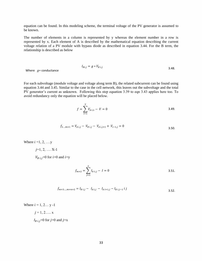
The number of elements in a column is represented by y whereas the element number in a row is
represented by x. Each element of A is described by the mathematical equation describing the current
voltage relation of a PV module with bypass diode as described in equation 3.44. For the B term, the
relationship is described as below
Where = conductance 3.48.
For each subvoltage (module voltage and voltage along term B), the related subcurrent can be found using
equation 3.44 and 3.45. Similar to the case in the cell network, this leaves out the subvoltage and the total
PV generator’s current as unknown. Following this step equation 3.39 to eqn 3.43 applies here too. To
avoid redundancy only the equation will be placed below.
3.49.
3.50.
Where =1, 2, ….y
=1, 2, …. X-1
=0 for =0 and =y
3.51.
3.52.
Where = 1, 2… y -1
= 1, 2….. x
=0 for =0 and =x
34
Using the set of equations 3.44 to 3.49, the unknown module voltages, including the PV generator’s
output current can be determine
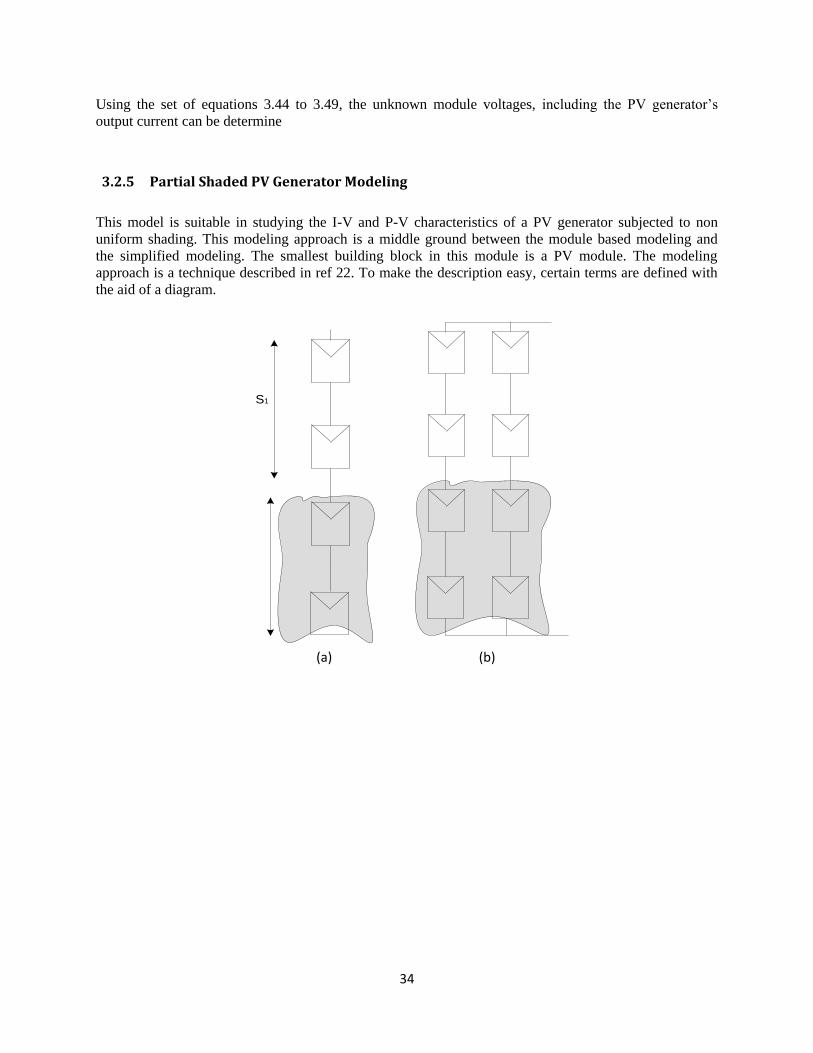
3.2.5 Partial Shaded PV Generator Modeling
This model is suitable in studying the I-V and P-V characteristics of a PV generator subjected to non
uniform shading. This modeling approach is a middle ground between the module based modeling and
the simplified modeling. The smallest building block in this module is a PV module. The modeling
approach is a technique described in ref 22. To make the description easy, certain terms are defined with
the aid of a diagram.
S1
(a) (b)

35
IT
G1 G2 G3 G4
VT
(c)
Figure 3.21 Terminology used in partial shaded PV generator modeling (a) string with 2 substring (b) group with two strings (c) PV generator
Modules that are connected in series that are subjected to the same operating condition are referred to as a
substring. This is shown as S1 in figure 3.23 (a). A “String” is then several such series connected
substrings that are subjected to different operating conditions (fig 3.23 (a)). Strings that have similar
shading pattern connected in parallel make up a “Group” (fig 3.23(b)). Various groups subjected to
different shading pattern connected in parallel make up the PV generator.
The irradiation level (E) and working temperature (T) of each substring created as a result of a specific
shading pattern over the PV generator should be known. Based on the E and T data and using a range of
voltage value between zero and open circuit voltage, the related current value is obtained using equation
3.47. This gives the I-V characteristics of a single module (with bypass diode) within a substring. Since a
substring is a series connection of modules under the same operating condition, the module’s voltage
value is upscaled by a factor equivalent to the number of module in the substring, while the current
remains the same. In that manner the I-V curve for all the substring making up a string can be acquired.
A string’s I-V curve is then created by the summation of the voltage value of each substring within the
string for a common current value. The group’s characteristics can be obtained by multiplying the current
value with a factor equivalent to the number of strings making up the group while the voltage value
remains the same. Finally for a common voltage value, the related current value from each group is
summed up to generate the I-V characteristics of the PV generator.

36
4 Solution
Background knowledge and possible methodology has been discussed in previous chapter. This chapter
covers the implementation part. The little knowledge that was gathered will be presented in a similar
order as carried out. This chapter first discusses the approach that was used to analyze the loss reduction
potential of the different inverter reconnection scheme discussed in part 3.1. The second part covers the
method chosen, the approaches taken and the challenges faced in modeling a large PV generator. Possible
methodologies implemented in the second part of this chapter are discussed in part 3.2.
4.1 Inverter Reconnection The loss reduction potential for different reconnection was evaluated in this section. The inverter
reconnection chosen for evaluation were
1. Classical inverter connection scheme: in this scheme it is assumed all output from the PV
generator was feed to a single DC bar and all nine inverters were always connected in parallel.
2. Master – Slave reconnection (minimum) scheme: here the number of slave inverters switched
is decided upon the maximum current loading of the inverters. This allows for minimum number
of inverters to be operated but each inverter is loaded to their maximum capacity.
3. Master –Slave reconnection (optimum) scheme: here the number of slave inverters connected
is based on the optimum loading of the inverters. When power output exceeds the optimum load
of connected inverters more slave inverters are switched in.
4. Team reconnection scheme: here input to adjacent inverters are checked, during low load
inverters are switched out and their dedicated input is redirected to the nearby inverters. During
high production, the output is directed to delegated inverters. Redirection to adjacent inverter is
done by checking the maximum current loading.
As a test case two locations were chosen, 1MW park layout located in Totana, Spain and another 1 MW
park located in Pöcking, Germany. The simulated generator output was used in the calculation. The plant
specification is presented in table below.
PV modules Zytech Monocrystalline Silicon 175 W
Inverters GAMESA 100 KW 9 Inverters
PV generator 18 Module/ String 37 String/ DC box 9 DC box (1 per inverter) 333 Strings in total 5994 Modules in total
Trackers Biaxial, 0.1 accuracy
Table 2 Specification of park layout in PVSyst for Totana, Spain and Pöcking, Germany
Two professional software program to simulate the output from a PV generator were at our disposal.
PVSyst was choosen for its relablity and wide use and INSEL due to its modular capabilities. PVSyst is
widely used as a simulation tool both for grid connected as well as standalone system. The user can
generate the annual irradiation level for a location from a large database of metrological sites. It also

37
provides the functionality of estimating the number of inverters needed based on the PV generator layout
(i.e. based on the selected module, no of series and parallel connection). The output from the simulation
result include loss breakdown among the various conversion stages, current and voltage output before the
inverter stage, power loss within the inverter and wiring loss are also accounted for. The connection
consideration, how losses are calculated and the coefficient used are not really clear when it comes to
PVSyst. INSEL on the other hand is more modular Software. It consists of building blocks for the
different component of a solar PV generator like modules, inverters. Blocks exist for generating
meteorological data for a location which provides the global irradiation on a horizontal surface and blocks
that can generate the irradiation on a tilted surface based on irradiation on a horizontal surface. All wiring
connection among the different blocks is done by the user which gives the user more freedom for
modification.
The models of both parks in PVSyst were already developed and the PV generator hourly output current
and voltage for the entire year was acquired by running the models.
For evaluating the first 3 inverter reconnection case, the result we simulate using PVSyst is acceptable
with little error. For performing any calculation for the fourth connection scheme, the output for each DC
box needed to be known first hand. This becomes a limitation since PVSyst only generates current and
voltage value for the entire generator. To mitigate these two simplified approaches were taken.
Approach 1: was to build a model in PVSyst taking parameters equal to part of the generator connected
to a single DC box. Table 3 below shows the used specification for simulation of a single DC box in
PVSyst.
PV modules Zytech Monocrystalline Silicon 175 W
Inverters GAMESA 100 KW 1 Inverters
Arrays 18 Module/ String 37 String 666 Modules in total
Trackers Biaxial, 0.1 accuracy
Table 3 Specification part of PV generator feeding a single DC box : PVSyst
The whole generator output was then taken by multiplying the current value acquired from PVsyst with
total number of DC box used by the PV generator. The result has limitations since it neglects any sort of
variation among DC box output.
Approach 2: The other sought solution was to use a more modular PV Generator simulation program
introduced earlier (INSEL). This is mainly because the program gives us the freedom to simulate the park
down to the DC box level. A screen shot of model is shown in fig 4.1.

38
Figure 4.1 Screen shot of Part of a 1MW PV generator: INSEL 8
The figure shows part of a model developed in INSEL 8 (the whole model is too big to get a full screen
shot). The block marked by a blue box represent part of the PV generator with 18 modules in series and
37 strings in parallel connected to a single maximum power point tracker. The modules are suntracking
modules. The portion marked with green also resembles the same arrangement but the modules used are
fixed angle modules. Different modules were used in the building the model was so as to create a
variation in the output among DC box. The suntracking modules have the capability to track the sun
position where as if fixed modules are chosen, then there is a specific tilt angle of the module that is
optimum for a particular location.
To resemble the situation where all the output from each DC box is feed into a single DC bar, another
model with a single maximum power point tracker for the entire park was also developed (not shown
here). The benefit of having individual maximum power point tracking for each DC box during team
operation can be more represented using this model. Using the models developed in both PVSyst and
Insel, the hourly current and voltage output of the PV generator system was generated.
The losses characteristics of the inverter used for all the case are taken from a data that is provided by the
inverter manufacturer. The inverter here is assumed to be a black box. We have a defined efficiency of the
inverter as a function of nominal load and input voltage provided in the datasheet. A program in
MATLAB is used to calculate the inverter power loss characteristics as a function of both input voltage
and current. Figure shows the loss power for a single 100 KW inverter.

39
Figure 4.2 Loss characteristics of a 100 KW Gamesa Inverter
For quantify the power loss binning is applied. The average power loss from the generator is then
presented as a function of voltage and current input. The input current can range from 0 to 1800 and this
is divided into 90 groups. While the voltage range from 430 to 670 V and this is divided into 24 groups. A
total of 2160 bins were created. The average of the values that falls within each group is calculated. The
average power for each bin is then calculated by multiplying the average value of the group making up
the bin. Average power value of each bin is represented below.

40
Figure 4.3 Average power output profile of PV generator.
The loss power for a single inverter for the voltage and current value of each bin is obtained through
interpolation. The total power loss for the generator system then can be calculated using the number of
inverters used and the loss power in each inverter. Following the procedure used in calculating the
inverter losses for the different inverter connection scheme will be explained, we start with the classical
inverter connection scheme
Classical inverter connection scheme: In this scheme, the average voltage and current value representing a bin is taken. The current value is
divided by the total inverters connected (in this case 9). This is assuming that each inverter shares the load
equally. The current and voltage value is used to determine the loss power within the inverter. The total
power loss is then the aggregate loss of each inverter.
Master – Slave reconnection (minimum) scheme: The average voltage and current value representing a bin is taken. From the current value, the number of
inverter to be operated for the bin is calculated by rounding the ratio between the bin average current
value and the max current capacity of the inverter to the nearest whole number. Once the number of
inverters to be operated is determined, the average current is divided by the number of operated inverters.
This is again assuming the number of operated inverters share the load current equally. The acquired
current value and voltage value is used to determine the loss power in a single inverter for the particular

41
bin. Total power loss for the bin is then the power loss in a single inverter multiplied by the number of
operated inverters for the bin.
Master –Slave reconnection (optimum) scheme: The average voltage and current value representing a bin is taken. From the current value, the lower
bound for the inverter combination for the bin is calculated by rounding the ratio between the bin average
current value and the max current capacity of the inverter to the nearest whole number. The upper bound
is set to the max number of inverters (in this case are 9). For each inverter combination in the range
corresponding input current for a single inverter is calculated. The power level is also calculated using the
average bin voltage and current for each inverter combination. The inverter combination with power level
closest to the optimum power level of a single inverter is chosen as the best inverter combination. Once
the number of operated inverter to be operated is determined, the bin average current value is divided by
the number of inverters operated to get a single inverter current value. The acquired current value and
average voltage value of the bin is used to determine the loss in a single inverter. The total loss for the bin
is calculated by multiplying the loss by the number of operated inverters.
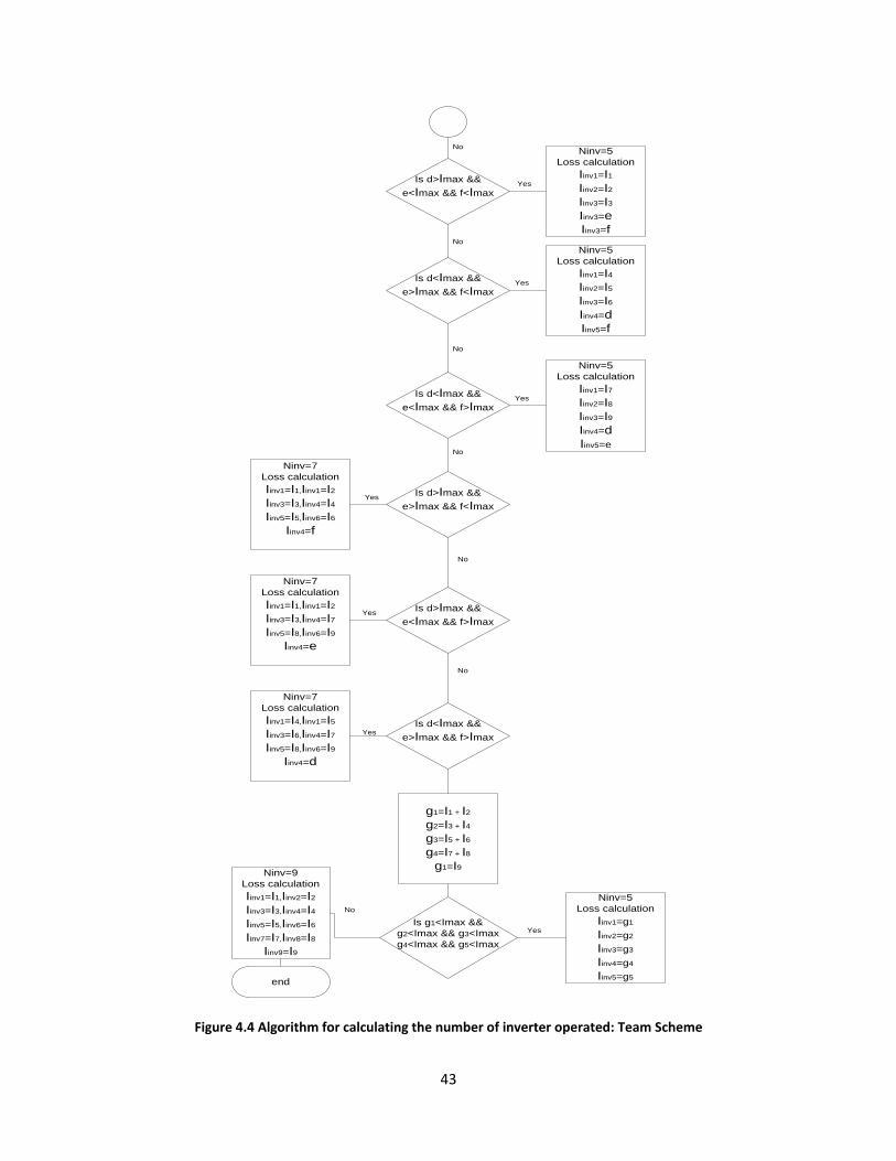
Team reconnection scheme: A flow chart is used to explain how the algorithm calculates the number of inverters operated for certain
input.. If not all inverters are operated, the voltage value input for each inverter need to be determined.
The program checks the average voltage value from each bin redirected to a single inverter and picks the
maximum. This way the highest possible average power is represented. The loss power for each inverter
is calculated individually and finally summed to get the total loss power for the bin.
Terms used in the flow chart
In = the current from the nth DC box, n=1,2,…9
Imax= maximum input current to a single inverter
Ninv=number of inverters

42
Imax=250
I1,I2,...In
Is b<Imax &&
c<Imax
Ninv=2
Loss calculation
Iinv1=b
Iinv2=c
a=∑Ii
n
i=1
Is a < ImaxNinv=1
Loss calculation
b=∑Ii
c=∑Ii
i=5
n
4
i=1
Is b>Imax &&
c<Imax
Is b<Imax &&
c<Imax
b1=I1+I2
b2=I3+I4
Is b1<Imax &&
b2<Imax
Ninv=3
Loss calculation
Iinv1=b1
Iinv2=b2
Iinv3=c
Is b1>Imax &&
b2<Imax
Ninv=4
Loss calculation
Iinv1=I1
Iinv2=I2
Iinv3=b2
Iinv4=c
Is b1<Imax &&
b2>Imax
Ninv=4
Loss calculation
Iinv1=I1
Iinv2=I2
Iinv3=b2
Iinv4=c
c1=I5+I6
c2=I7+I8
c3=I9
Is c1<Imax &&
c2<Imax &&
c3<Imax
Ninv=4
Loss calculation
Iinv1=c1
Iinv2=c2
Iinv3=c3
Iinv4=b
Ninv=4
Loss calculation
Iinv1=I5
Iinv2=I6
Iinv3=c2
Iinv4=c3
Is c1>Imax &&
c2<Imax &&
c3<Imax
Is c1<Imax &&
c2>Imax &&
c3<Imax
Ninv=4
Loss calculation
Iinv1=I7
Iinv2=I8
Iinv3=c1
Iinv4=c2
Yes
No
No
No No
Yes
Yes Yes
Yes
Yes
NoNo
YesYes
Yes
Yes
No
d=∑Ii
e=∑Ii
f=∑Ii
i=1
i=4
i=7
3
6
9
No
No
No
Is d<Imax &&
e<Imax && f<Imax
Ninv=3
Loss calculation
Iinv1=d
Iinv2=e
Iinv2=f
Yes
No
43
Is d>Imax &&
e<Imax && f<Imax
Ninv=5
Loss calculation
Iinv1=I1
Iinv2=I2
Iinv3=I3
Iinv3=e
Iinv3=f
Is d<Imax &&
e>Imax && f<Imax
Ninv=5
Loss calculation
Iinv1=I4
Iinv2=I5
Iinv3=I6
Iinv4=d
Iinv5=f
Is d<Imax &&
e<Imax && f>Imax
Ninv=5
Loss calculation
Iinv1=I7
Iinv2=I8
Iinv3=I9
Iinv4=d
Iinv5=e
Is d>Imax &&
e>Imax && f<Imax
Ninv=7
Loss calculation
Iinv1=I1,Iinv1=I2
Iinv3=I3,Iinv4=I4
Iinv5=I5,Iinv6=I6
Iinv4=f
Is d>Imax &&
e<Imax && f>Imax
Ninv=7
Loss calculation
Iinv1=I1,Iinv1=I2
Iinv3=I3,Iinv4=I7
Iinv5=I8,Iinv6=I9
Iinv4=e
Is d<Imax &&
e>Imax && f>Imax
Ninv=7
Loss calculation
Iinv1=I4,Iinv1=I5
Iinv3=I6,Iinv4=I7
Iinv5=I8,Iinv6=I9
Iinv4=d
g1=I1 + I2
g2=I3 + I4
g3=I5 + I6
g4=I7 + I8
g1=I9
Is g1<Imax &&
g2<Imax && g3<Imax
g4<Imax && g5<Imax
Ninv=5
Loss calculation
Iinv1=g1
Iinv2=g2
Iinv3=g3
Iinv4=g4
Iinv5=g5
Ninv=9
Loss calculation
Iinv1=I1,Iinv2=I2
Iinv3=I3,Iinv4=I4
Iinv5=I5,Iinv6=I6
Iinv7=I7,Iinv8=I8
Iinv9=I9
end
No
No
No
No
No
No
No
Yes
Yes
Yes
Yes
Yes
Yes
Yes
Figure 4.4 Algorithm for calculating the number of inverter operated: Team Scheme

44
4.2 PV generator modeling
4.2.1 Module Based Modeling
The implementation was started with the module based model. The precondition was previously done
thesis work on PV module modeling based on the one diode model. To generate a varying irradiation
condition, a solution in reference 13 was used. It relates the passing of a cloud to a change in the short
circuit current. The author in his approach, calculates the distance between the solar cell at a
certain time instance, using equation 4.1
4.1.
Where = Speed of cloud
= time instane
Since the irradiance is proportional to the short circuit current, the effect of a passing cloud on a solar
array can be modeled as a change in the short circuit current. The author defines a relationship between
the short circuit current at STC and short circuit of the specific cell using a sin function as shown below
4.2.
Taking the average speed of a cloud to be 10m.p.h, the variation on a 10 by 10 configuration is plotted in
MATLAB.
Figure 4.5 Changing irradiation effect due to a passing cloud on a 10 by 10 configuration: each for a time
instance ti

45
Although the above equation as stated in paper is for PV cell in a module, it is acceptable to use it for a
module level based on our assumption that each cell in the module based modeling is subjected to the
same irradiation level. Although it doesn’t reflect real time situation, the result can be taught of creating a
random irradiation along a surface which could be similar to that created by a passing cloud.
The problem was started at a small level having 4 modules in total, two modules in series forming a string
and two strings in parallel. Equation 3.47 is used to define voltage relation in each mesh. Equation 3.48 is
used to define each string output contribution to the total current. Equation 3.49 is used to write the
current for two nodes. The current output for each module is calculated by passing voltage value to a
function that uses the one diode mathematical model representation of the module. Fsolve in MATLAB
was used to solve the equations for voltage values and total current. Unfortunately the program reaches
max iteration before it can solve the problem.
The PV generator was up scaled to contain 6 modules and another solution was tried. Two conditions
were used to define an objective function
Condition1: The same current flows through all modules in the string.
Condition 2: The sum of voltage from each module in a string gives the terminal voltage
The objective function defined in MATLAB is shown below.
x(1)=(I1 -I2)^2+(I2-I3)^2+(I3-I1)^2; x(2)=(I4-I5)^2 + (I5-I6)^2+(I6-I4)^2; x(3)=(Vt -(V(1)+V(2)+V(3)))^2 + (Vt - (V(4) + V(5) + V(6)))^2;
I1, I2 and I3 are current produced by module 1, module 2 and module 3 making up the first string. I4, I5
and I6 are current produced by module 4, module 5 and module6 making up the second string. The
objective function is then to minimize the sum of x. A function that uses the Levenberg Marquardt
algorithm to arrive at a solution found from the web was used. The result didn’t converge to a solution.
As a last resort, the current voltage relationship was redefined, to define the objective function. Index is
used to differentiate the voltage value and current output of a module. “n” indicates the number of
modules connected in series to form a string and “m” indicates the number of strings connected in
parallel. Based on the condition that the difference of the current among series connected module should
be zero a set of equation is defined
4.3.
Where i=1,2,…n-1 and j=1,2,….m
The voltage output of a string should equal the total voltage of the PV generator
4.4.
For j=1,2,…m
=voltage drop across blocking diode

46
The model assumes a bypass diode exists in parallel with each module and a blocking diode in series with
each string. The total current of the PV generator can be expressed as the contribution of current from
each string.
4.5.
Where and corresponds to the PV generator output at the terminal. The results from using this
approach is presented in part 5.5
4.2.2 Simplified PV generator modeling
Each module along the string is subjected to the same operating condition and is assumed to contribute
equally for the value of the terminal voltage. The developed model was PV generator with a 1MW
capacity. Each string consists of 18 modules in series and 360 strings in parallel. Two layout of the PV
generator was tried.
First layout was the central layout where all the output from each string is assumed to feed a single DC
bar. All strings are operated at the DC bar voltage. The second layout was a string layout where the park
is grouped into 2 groups, each group with 180 strings in parallel. Each group has its own independent
operating voltage. The algorithm in both layouts takes the percentage shading value as an input from the
user.
The purpose was to actually simulate the PV generator’s output when subjected to shading condition. A
set of irradiation values that are incident upon the PV generator module needed to determined. As a
simplification of a very complex process, the assumption taken was that two irradiation levels exists; one
representing unshaded condition and the other representing a shaded condition. For the sake of not
choosing random value for the irradiation level, the values were taken to be the hourly global in plane
irradiation and the diffused inplane irradiation of a particular area. An excel file is made to provide the
algorithm with two irradiation level for solar hours within a year.
The algorithm asks the user to choose between central or team layout. If a central set up is selected, the
program proceeds as follows. Initially the algorithm solves to find the operating voltage of the PV
generator. For this it calls a function to calculate the MPP of the PV generator for the provided shading
condition.
The function goes to computes for the unshaded portion first and saves the data for further calculation. It
starts at a string level, by taking the hourly irradiation level to generate the I-V characteristics of the
string. Using the percentage shading data provided from the user, the portion of the whole park that isn’t
shaded is determined. Based on this value, the I-V curve of unshaded group is determined and saved. The
algorithm does the above 3 step for every global irradiation level provided in the excel sheet. To reduce
the computation and since no energy is harnessed during night time, no computation is done during night
hours.
Next, it calculates for the shaded portion with the similar procedure as that of the unshaded portion but
taking the diffused inplane irradiation value into account. The total I-V characteristic of the PV generator
for each hour is then computed by summing the contribution from the shaded and unshaded portion.
Based on the generated hourly I-V curve of the PV generator, the PV generator’s MPP voltage values can
be calculated for each hour. The algorithm then returns the hourly operating point for the range hourly
irradiation level provided in the excel spread sheet assuming that the PV generator is always operated at

47
its MPP. The program then calls a second function that takes the saved hourly operating point voltage to
generate the operating current for the defined shading condition and irradiation level.
When the user selects the team layout of the park, the algorithm assumes the park is divided into two parts
each with 180 strings that operate independently. It should be pointed out that the unshaded part in each
portion of the PV generator are subjected to same irradiation level (i.e. global inplane irradiation). The
above statement also holds for the shaded part. The two parts thus differ only in the percentage shading
provided by the user. The algorithm then calls a function that performs the MPP tracking to determine
each portion operating point. What the function does is perform the same procedure explained above but
does it for the two parts separately. From the function the operating voltage for the two parts is generated
and saved. The algorithm then calls another function to compute the operating current for the saved
operating voltage point. It does this for the two portion of the PV generator separately. Finally the
algorithm saves the generated hourly current and voltage value into an excel sheet. Another down side of
this method that is not stated in chapter 3 is that it is really computational expensive.
4.2.3 Partially shaded PV Generator Modeling
The Algorithm can intake a shading pattern from the user and produce I-V characteristics curve for one
instance of time. The implementation of the algorithm in MATLAB is as follows. The program starts by
taking the shading pattern from the user. The outlook is shown below
///////////////////////////////////////////////////////////////////////////////////////////////////////////////////// please enter the number of groups 4 Enter no of substring for group No1 =3 Enter No of module in each substring enclosed in square bracket([])separated by comma = [8,6,4] enter irradiation for each substring enclosed in square bracket([])separated by comma = [1,.5,.2] Enter the temp for each substring enclosed in square bracket([])separated by comma = [25,21,18] Enter no of string for group No1 =80 Enter no of substring for group No2 =2 Enter No of module in each substring enclosed in square bracket([])separated by comma = [12,6] enter irradiation for each substring enclosed in square bracket([])separated by comma = [1,2] Enter the temp for each substring enclosed in square bracket([])separated by comma = [25,18] Enter no of string for group No2 =100 Enter no of substring for group No3 =2 Enter No of module in each substring enclosed in square bracket([])separated by comma = [16,2] enter irradiation for each substring enclosed in square bracket([])separated by comma = [1,.2] Enter the temp for each substring enclosed in square bracket([])separated by comma = [25,18] Enter no of string for group No3 =120 Enter no of substring for group No4 =1 Enter No of module in each substring enclosed in square bracket([])separated by comma = [18] enter irradiation for each substring enclosed in square bracket([])separated by comma = [1] Enter the temp for each substring enclosed in square bracket([])separated by comma = [25] Enter no of string for group No4 =60 /////////////////////////////////////////////////////////////////////////////////////////////////////////////////////
It first calculates and generates the I-V curve of all substrings with in a group. This is achieved by up
scaling the I-V characteristics of a module under the same operating condition as the substring. The
program performs the above step for each substring within the string. Each string I-V characteristics is
generated from the I-V curve of the substrings. The program does an interpolation of the voltage value for
a current range from zero to the resulting maximum short circuit current among the substrings. The
interpolated voltage value for each point in the current range is summed to generate the I-V curve of the
string. The group I-V characteristic is then achieved by up scaling the current value of the string by a

48
factor equal to the total number of strings making up the group. Then the program goes to interpolate the
current value for a common voltage for each group. Then the program generates the I-V curve for the
generator by summing the current contribution of each group for a common voltage value. The voltage
range is set from zero to maximum open circuit voltage from the group.
The down side of this model is that it can only generate the I-V curve of the PV generator for a single
instant of time. The user needs to input the shading pattern for each instant. It is a good approach to
visualize the effects of partial shading on the general characteristic curve of a PV generator. The
implementation alongside little description is presented in section 5.4. In section 3.2.5, terms used to
describe the parts of the generator using this modeling approach was described. The 4 curves below
shows the I-V characteristics of each group. A group’s operating condition defines part of the total
operating condition of the PV generator at a time instance t. The array output is thus the aggregate
contribution from each group
Figure 4.6 I-V characterisitics of individual group corresponding to a shading condition

49

50
5 Results The results are presented in accordance to the steps followed in the solution part of this report. A small
description in each section is included. Analysis is presented alongside results. The first part of the
chapter presents the result for the loss calculation for the inverter reconnection scheme. The second part
5.1 Loss calculation for different Inverter Reconnection Scheme
In the initial stage two locations were chosen, a 1 MW solar power plant in Totana, Spain and a similar
1MW plant in Germany. The choice of location is because both region have the high potential with
regards to solar irradiation [27]. The data for the park is simulated in PVSyst V 5.12 . The extracted data
from PVSyst was the array’s hourly current and voltage output for an entire year. Similarly the hourly
current and voltage for the Poking solar power plant in Germany was extracted. The chosen size and
number of inverter is based on the actual no of inverters employed in the plant. But due to the missing
efficiency data of specific inverter used, a 100KW inverter from Gamesa was used for the calculation.
First batch of test was based on hourly current and voltage output generated using PVSyst. The result will
be presented side by side for the individual park.
The PV array voltage and current distribution for the park in Totana, Spain and for the park Poking in
Germany is plotted in figure 5.1 and 5.2 below
Figure 5.1 Histogram showing yearly time distribution : Totana, Spain

51
Figure 5.2 Histogram showing yearly time distribution, Pöcking, Germany
The metanom data that is used in PVSyst runs from jan 1990- December 1990. This is one of the down
sides of using PVSYst. Assuming the data from PVSyst is fairly accurate, the losses for the different
inverter reconnection scheme is computed.
Result for inverter reconnection Scheme 1
In this scheme, there exists a single DC bar and all the array output is feed to the DC bar. The 9 inverters
are then connected to the DC bar and they share the load current equally. All the inverters stay connected
during the entire operating hours
Figure 5.3 Cumulative powerloss distribution when all nine inverters are operated: Totana Park

52
Figure 5.4 Cumulative powerloss distribution when all nine inverters are operated: Pöcking Park
When the PV generator’s output is low, all the inverters stay connected and share the output equally.
During low PV generator output each inverter works in its low efficiency region and therefore the
cumulative losses appear to be larger
Result for inverter reconnection Scheme 2:
In this scheme, there exists a single DC bar and all the array output is feed to the DC bar. The number of
inverters that are operated is based on the current output of the PV generator. Here each inverter that is
connected is operated to their maximum current capacity. In other words, each time, minimum no of
inverters are connected and each inverter is forced to operate to their maximum current loading. The
power loss distribution for this scheme is shown below.
(a)

53
(b)
Figure 5.5 the cumulative powerloss distribution when each inverter loaded to max current capacity.(a) Totana Park, Spain (b)Poking Park, Germany
At low PV generator output inverters are disconnected while the connected inverters are loaded to their
maximum current capacity. When the output from the generator exceeds the connected inverter’s
capacity, more inverters are switched in. comparing figure 5.4 and 5.5, a lower power loss during low PV
generator output is mainly because the lower number of inverters operated (which indicates less additive
losses). During maximum generation, the loss distribution is similar since the operated numbers of
inverters are the same in both schemes.
Result for inverter reconnection Scheme 3:
In this scheme, there exists a single DC bar and all the array output is feed to the DC bar. The PV
generators output is shared among the inverters so that each inverters are loaded to their optimum
operating point. No inverter is loaded to the maximum operating capacity. The value of the optimum
power used for the computation is the one provided by the manufacturer. The power loss distribution for
this case is shown figure 5.6.

54
. (a)
(b)
Figure 5.6 Cumulative powerloss distribution when each inverter loaded to optimum power capacity.(a) Totana Park, Spain (b)Poking Park, Germany
The steps observed in the power loss distribution diagram is an indicative of the increase in the number of
inverters operated.
Comparison between the 3 schemes can be done by a means of annual energy loss in the system. During
the night, when the inverters are disconnected a constant loss of 35W as specified by the manufacturer is
accounted for.

55
(a) (b)
Figure 5.7 The Energy loss for the 3 reconnection scheme (a)Totana park, Spain (b)Pöcking Park, Germany
The result indicates the scheme where all inverters are operated as having the max loss. Among the
master slave operation, the scheme where inverters are switched based on their optimum capacity bring
up the least loss in both parks.
Result for inverter reconnection Scheme 4:
In this scheme, unlike the others mentioned above no common DC bar exists for all inverters. Each
inverter is operated individually during high output. At low generator output, the input to the inverter can
then be rerouted so that lower numbers of inverters are operated. For ease of reference the scheme will be
called team concept. To be able to represent the powerloss distribution using the team concept and at the
same time be able to compare the result with the rest of the scheme, the output of the PV generator for a
single individual inverter was generated by PVSyst. The approach is explained in section 4.1. The
histogram showing yearly time distribution for a single inverter input is shown figure 5.8.
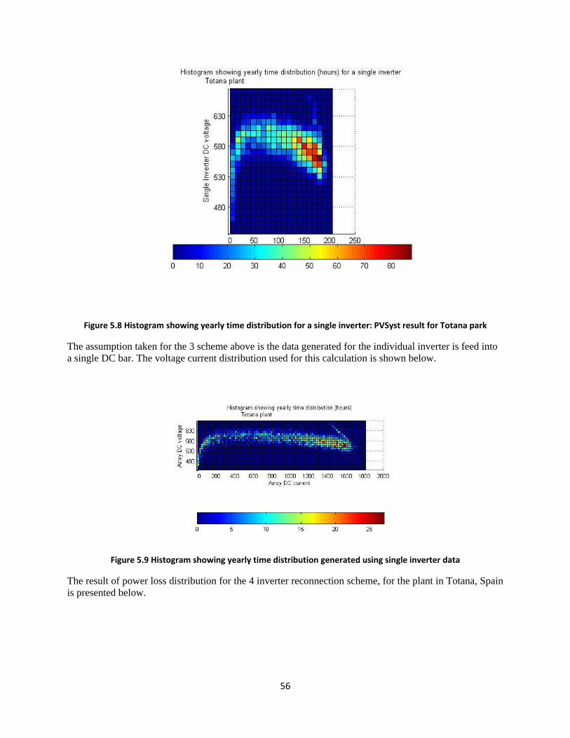
56
Figure 5.8 Histogram showing yearly time distribution for a single inverter: PVSyst result for Totana park
The assumption taken for the 3 scheme above is the data generated for the individual inverter is feed into
a single DC bar. The voltage current distribution used for this calculation is shown below.
Figure 5.9 Histogram showing yearly time distribution generated using single inverter data
The result of power loss distribution for the 4 inverter reconnection scheme, for the plant in Totana, Spain
is presented below.

57
(a) (b)
(c)

58
(d)
Figure 5.10 Cumulative powerloss distribution for 4 inverter reconnection scheme in Totana plant(a)All inverters
connected always(b)inverter reconnection based on max current loading(c)inverters reconnection based on optimum loading of inverter(d)team Concept
Part (d) in figure 5.10, since output of a individual inverters can be rerouted to adjacent inverters, the
possible combination steps are a single inverter, two inverters, 3 inverters, 5 inverters and 9 inverters. The
cumulative power loss is therefore the sum of losses in each inverter that is operated.
The energy loss per year is plotted out as a tool for comparison.
Figure 5.11 The Energy loss for the 4 reconnection scheme, Totana Park, Spain
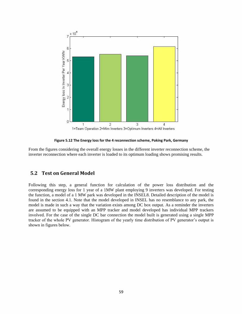
59
Figure 5.12 The Energy loss for the 4 reconnection scheme, Poking Park, Germany
From the figures considering the overall energy losses in the different inverter reconnection scheme, the
inverter reconnection where each inverter is loaded to its optimum loading shows promising results.
5.2 Test on General Model Following this step, a general function for calculation of the power loss distribution and the
corresponding energy loss for 1 year of a 1MW plant employing 9 inverters was developed. For testing
the function, a model of a 1 MW park was developed in the INSEL8. Detailed description of the model is
found in the section 4.1. Note that the model developed in INSEL has no resemblance to any park, the
model is made in such a way that the variation exists among DC box output. As a reminder the inverters
are assumed to be equipped with an MPP tracker and model developed has individual MPP trackers
involved. For the case of the single DC bar connection the model built is generated using a single MPP
tracker of the whole PV generator. Histogram of the yearly time distribution of PV generator’s output is
shown in figures below.

60
Figure 5.13 Histogram showing the yearly time distribution of PV generator :model built in INSEL 8
For the case where individual MPP trackers were employed, the yearly time distribution for some DC box
is shown below. 9 DC box exists, out of which 4 DC box each aggregating 37 string with sun tracking
modules. The remaining 5 DC box each aggregating 37 strings with fixed angle module. The tilt angle
for the modules within a single DC box was uniform but a variation was introduced among modules of
different DC box. The used tilt angles for the modules were 33.7 deg, 60 deg, 40 deg, 22 deg and 15 deg
(not all is presented in the figures)

61
Figure 5.14 Histogram showing the yearly time distribution: single DC box feed from string of suntracking
modules
Figure 5.15 Histogram showing the yearly time distribution: single DC box feed from string of fixed modules with
33.7 deg tilt

62
Figure 5.16 Histogram showing the yearly time distribution: single DC box feed from string of fixed modules with
60 deg tilt
From the model, the generated PV generator voltage and current with individual MPP tracker for every 37
strings connected in parallel (which corresponds to one DC box) is used to test the team concept. On the
other hand the generated array voltage and current for the whole PV generator with a single MPP tracker
was used to test the 3 other inverter reconnection scheme. The result is presented below
(a) (b)
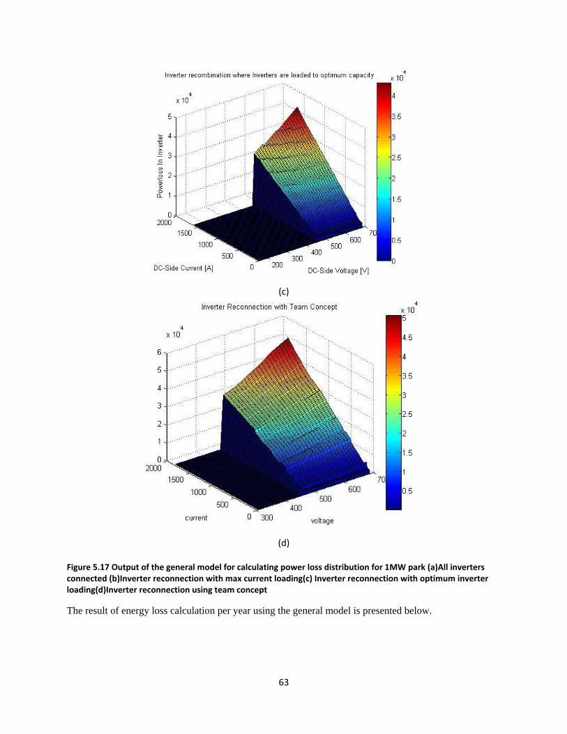
63
(c)
(d)
Figure 5.17 Output of the general model for calculating power loss distribution for 1MW park (a)All inverters connected (b)Inverter reconnection with max current loading(c) Inverter reconnection with optimum inverter loading(d)Inverter reconnection using team concept
The result of energy loss calculation per year using the general model is presented below.

64
Figure 5.18 The Energy loss for the 4 reconnection scheme:Test for General model
It is observed that as the combination of inverter connection during the team operation is increased the
energy loss also increases. In theory the team concept gives the flexibility of operating less number of
inverters when output is lower. The downside is the inverters that are switched out can’t freely be chosen
since rerouting is only possible among adjacent inverters. This limits rerouting options if further apart
portion experience lower production.
The condition where inverters are operated to the maximum capacity shows a promising result as
compared to team operation is from the fact the max number of inverters operated was 7 inverters. The
master slave reconnection scheme based on maximum current loading can be good choice where the yield
of the park is low compared as compared to its installed capacity. The master slave operation with
inverters loaded to their optimum loading shows the best result.
5.3 Simplified PV Generator Modeling for Inverter reconnection Analysis The data generated using the simplified PV generator model was used to calculate the power loss
distribution and total energy loss for the 4 inverter reconnection schemes discussed pervious section
The simplified PV generator model developed has two options, the central or team. Assumption taken is
that all modules with in a string are subject to the same shading condition and same temperature. The
selection menu is shown below
The header of the program used to simulate the array is shown below

65
%% To generate output of an array under shading condition
% % Assumption : %(1) Plant is divided into 2 parts, each part consists of 180 strings % connected in parallel. Each string has 18 modules in series %(2)All modules along the string is subjected to uniform % irradiation %(3)Temperature effect between shaded and un shaded portion isn't considered % % INSTRUCTION: % - Choose option "central" for the condition that the entire output of the % array is feed into a single DC bar. % - Choose Option "Team" for the condition that 2 DC bar exist and the output % from first 180 parallel strings are connected to the first DC bar and the % output of the last 180 strings is connected to the 2nd DC bar. % - The current and voltage output is saved in the excel file with a file % name "Result--%shading.xls" for option central and file name % "ResultArrayPart1 --%shadingArrayPart2 --%shading"
The irradiation data taken for result presented here is a generated data of the global in plane and the
diffused in plane for a location with latitude of 36.3. The header file of the program used for power loss
distribution is shown below
%% To make Loss Calculation for Different Inverter Reconnection % Case Considered: 1MW plant % % This algorithm for loss calculation using data generated from an array % model. The array model is static with two options Central or Team. The % result generated using the "Central" option is used when inverter % reconnection which involves a single DC bar. The result generated using % "Team" option is used where inverters are connected independently. % No of Inverters=2, 500 KW Inverters
The generated data used for the calculation considered a 30% shading of the whole PV generator when
the Central option was chosen. To generate equivalent shading, a 20% shading on the first 180 string and
a 40% shading in the 2nd 180 string was used when option “Team” was selected. The program plots the I-
V and P-V Curve based on the shading condition and the irradiation level. As a demo the program is run
for one day with 30% shading of the array. The plots are presented below

66
Figure 5.19 PV generator I-V curve for a day with 30% shading: simplified PV generator model used (central
option)
Figure 5.20 PV generator P-V curve for a day with 30% shading: simplified PV generator model used (central
option)
The program then continues to compute the operating point current of the array using the MPP voltage as
the operating voltage. The acquired current voltage value for each pair of irradiation value is then saved
on to an excel file. The generated I-V and P-V curve of the same day using the team option is shown
figure 5.21

67
(a)
(b)

68
(c)
(d)
Figure 5.21 Generated I-V and P-V curve for 20% shading of part 1 and 40% shading on part 2. (a) I-V curve for part 1 (b) P-V curve for part 1 (C) I-V curve of part 2 (d) P-V curve of part 2
The yearly time distribution of the data generated is shown below. Figure 5.22 shows the result when the
central option is chosen whereas figure 5.23 shows the result when the team option is selected

69
Figure 5.22 The yearly time distribution generated in MATLAB using Central option
(a) (b)
Figure 5.23 Shows the yearly time distribution generated in MATLAB using Team option (a) first 180 strings with 20% shading and (b) last 180 string with 40% shading
Quantifying the power loss for the 4 inverter reconnection scheme discussed the power loss distribution
as a function of voltage and current is plotted below. The inverter employed are 2, 500 KW inverters.
(a) (b)
Figure 5.24 Power loss distribution based on data generated using simplified PV generator model (a) All inverters always connected (b) Inverter reconnection with max current loading
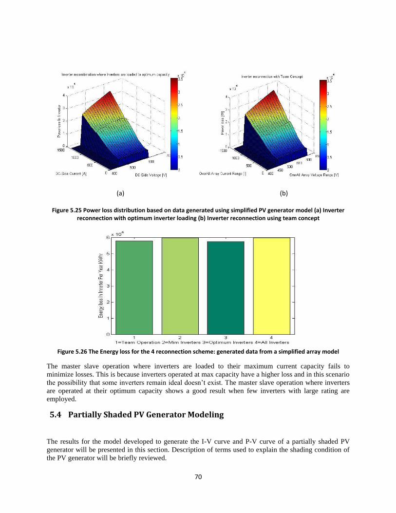
70
(a) (b)
Figure 5.25 Power loss distribution based on data generated using simplified PV generator model (a) Inverter reconnection with optimum inverter loading (b) Inverter reconnection using team concept
Figure 5.26 The Energy loss for the 4 reconnection scheme: generated data from a simplified array model
The master slave operation where inverters are loaded to their maximum current capacity fails to
minimize losses. This is because inverters operated at max capacity have a higher loss and in this scenario
the possibility that some inverters remain ideal doesn’t exist. The master slave operation where inverters
are operated at their optimum capacity shows a good result when few inverters with large rating are
employed.
5.4 Partially Shaded PV Generator Modeling
The results for the model developed to generate the I-V curve and P-V curve of a partially shaded PV
generator will be presented in this section. Description of terms used to explain the shading condition of
the PV generator will be briefly reviewed.

71
Substring: is composed of series connected modules that are subjected to the same operating condition
(equal irradiation and temperature)
String: composed of series connection of substrings which are subjected to different operating condition.
Group: string that have similar shading pattern is termed as group
Array: then several group elements with their respective shading pattern which are connected in parallel
making up the solar array
Group No 1 2 3 4 Total
No of substring
3 2 2 1 4
Module in substring
[8 ,6, 4] [12, 6] [16, 2] [18]
Irradiation [1, .5, .2] [1, .2] [1, .2] [1]
temperature [25, 21, 18] [25, 18] [25, 18] [25]
No of String in group Group
80 100 120 60 360
Table 4 Shading description input to program: time instant t1
The table above describes the irradiation over the PV generator for one instance of time. The values that
is presented in the table is in the same format that is input into the m-file that generates the characteristics
I-V and P-V curve of the PV generator. The outlook in MATLAB looks like this
////////////////////////////////////////////////////////////////////////////////////////////////////////////// please enter the number of groups 4 Enter no of substring for group No1 =3 Enter No of module in each substring enclosed in square bracket([])separated by comma = [8,6,4] enter irradiation for each substring enclosed in square bracket([])separated by comma = [1,.5,.2] Enter the temp for each substring enclosed in square bracket([])separated by comma = [25,21,18] Enter no of string for group No1 =80 Enter no of substring for group No2 =2 Enter No of module in each substring enclosed in square bracket([])separated by comma = [12,6] enter irradiation for each substring enclosed in square bracket([])separated by comma = [1,2] Enter the temp for each substring enclosed in square bracket([])separated by comma = [25,18] Enter no of string for group No2 =100 Enter no of substring for group No3 =2 Enter No of module in each substring enclosed in square bracket([])separated by comma = [16,2] enter irradiation for each substring enclosed in square bracket([])separated by comma = [1,.2] Enter the temp for each substring enclosed in square bracket([])separated by comma = [25,18] Enter no of string for group No3 =120 Enter no of substring for group No4 =1 Enter No of module in each substring enclosed in square bracket([])separated by comma = [18] enter irradiation for each substring enclosed in square bracket([])separated by comma = [1] Enter the temp for each substring enclosed in square bracket([])separated by comma = [25] Enter no of string for group No4 =60 //////////////////////////////////////////////////////////////////////////////////////////////////////////////
The generated I-V curves of all substrings within a string of all 4 Group is shown in figure 5.27

72
(a) (b)
Figure 5.27 Individual I-V curve of substrings making up a string (a) Group 1 (b) Group 2
The blue curve in figure 5.27 (b) is the resulting I-V curve of 8 modules in series subjected to irradiation
equal to 1000W/m2 at the temperature of 25 degrees. The pink curve on the same fig represents the I-V
curve of 4 modules in series subjected to irradiation of 200W/m2 at a temperature of 18 degree. Curves
for group 3 and 4 are shown below. Note that in group 4 (fig 5.28 (b)), all modules receive the same
irradiation therefore curve in blue represent I-V curve of 18 modules in series subjected to irradiation of
1000W/m2 and temperature of 25 degree.
(a) (b)
Figure 5.28 Individual I-V curve of substrings making up a string (a) Group 3 (b) Group 4
The resultant I-V curve for each group is presented in figure 5.29

73
(a) (b)
(c) (d)
Figure 5.29 Individual I-V curve of each group making the PV generator (a) Group 1 (b) Group 2 (c) Group 3 (d) Group 4
The resultant characteristics I-V curve and P-V curve for the PV generator system is shown in figure 5.30

74
Figure 5.30 The I-V curve of the PV generator for a shading condition described in table 4(left),P-V curve of the PV generator (right)
The output from the program is presented below
%%%%%%%%%%%%%%%%%%%%%%%%%%%%%%%%%%%%%%%%%%%%%%%%%%%%%%%%%%% % Generated operating point value %---------------------------------------------------------------- % Array Operating Point current =1292.2688 A % Array Operating Point voltage = 456 V % Array Operating Point Power = 589.2746 KW %%%%%%%%%%%%%%%%%%%%%%%%%%%%%%%%%%%%%%%%%%%%%%%%%%%%%%%%%%%
To create a simplified dynamic shading scenario, a shifting shading condition for 5 time instance
following the one illustrated above was simulated. The shading condition was made to shift along the PV
generator system until condition of no shading. Table 5 to table 9, describe the shading information that is
feed to the m-file to generate the I-V,P-V curve , operating point voltage(V) , Current( I) and power
Group No 1 2 3 4 Total
No of substring 2 3 2 2 4
Module in substring
[10, 8] [8 ,6, 4] [12, 6]
[16, 2]
Irradiation [1, .5] [1, .5, .2] [1, .2] [1, .2]
temperature [25, 21] [25, 21, 18] [25, 18] [25, 18]
No of String in Group
60 80 100 120 360
Table 5 Shading description input to program: time instant 2(t2)

75
Group No 1 2 3 4 Total
No of substring 1 2 3 2 4
Module in substring
[18] [10, 8] [8 ,6, 4] [12, 6]
Irradiation [1] [1, .5] [1, .5, .2] [1, .2]
temperature [25] [25, 21] [25, 21, 18] [25, 18]
No of String in Group
120 60 80 100 360
Table 6 Shading description input to program: time instant 3 (t3)
Group No 1 2 3 Total
No of substring 1 2 3 3
Module in substring [18] [10, 8] [8 ,6, 4]
Irradiation [1] [1, .5] [1, .5, .2]
temperature [25] [25, 21] [25, 21, 18]
No of String in 220 60 80 360
Group
Table 7 Shading description input to program: time instant 4 (t4)
Group No 1 2 Total
No of substring 1 2 2
Module in substring [18] [10, 8]
Irradiation [1] [1, .5]
temperature [25] [25, 21]
No of String in 300 60 360
Group
Table 8 Shading description input to program: time instant 5 (t5)

76
Group No 1 Total
No of substring 1 1
Module in substring [18]
Irradiation [1]
temperature [25]
No of String in 360 360
Group
Table 9 Shading description input to program: time instant 6 (t6)
The Generated operating point value, the I-V and P-V curve of the PV generator for the each time
instance is shown in the rest of this section
Time instance 2
---------------------------------------------------- %%%%%%%%%%%%%%%%%%%%%%%%%%%%%%%%%%%%%%%%%%%%%%%%%%%%%%%%%%% % Generated operating point value %---------------------------------------------------------------- % Array Operating Point current =1428.9802 A % Array Operating Point voltage = 454.3 V % Array Operating Point Power = 649.1857 KW %%%%%%%%%%%%%%%%%%%%%%%%%%%%%%%%%%%%%%%%%%%%%%%%%%%%%%%%%%%
(a) (b)
Figure 5.31 The I-V curve of the PV generator for time instance 2 described in table 5(left),P-V curve of the PV generator (right)

77
Time instance t3
---------------------------------------------------- %%%%%%%%%%%%%%%%%%%%%%%%%%%%%%%%%%%%%%%%%%%%%%%%%%%%%%%%%%% % Generated operating point value %---------------------------------------------------------------- % Array Operating Point current =1430.3112 A % Array Operating Point voltage = 455.7 V % Array Operating Point Power = 651.7928 KW %%%%%%%%%%%%%%%%%%%%%%%%%%%%%%%%%%%%%%%%%%%%%%%%%%%%%%%%%%%
(a) (b)
Figure 5.32 (a)The I-V curve of the PV generator for time instance 3 described in table 6(b) P-V curve of the PV generator
Time instance t4
%%%%%%%%%%%%%%%%%%%%%%%%%%%%%%%%%%%%%%%%%%%%%%%%%%%%%%%% % Generated operating point value %---------------------------------------------------------------- % Array Operating Point current =1313.365 A % Array Operating Point voltage = 629.7 V % Array Operating Point Power = 827.0259 KW %%%%%%%%%%%%%%%%%%%%%%%%%%%%%%%%%%%%%%%%%%%%%%%%%%%%%%%%

78
(a) (b)
Figure 5.33 (a)The I-V curve of the PV generator for time instance 4 described in table 7(b) P-V curve of the PV generator
Time instance 5
---------------------------------------------------- %%%%%%%%%%%%%%%%%%%%%%%%%%%%%%%%%%%%%%%%%%%%%%%%%%%%%%%% % Generated operating point value %---------------------------------------------------------------- % Array Operating Point current =1486.6802 A % Array Operating Point voltage = 618.6 V % Array Operating Point Power = 919.6604 KW %%%%%%%%%%%%%%%%%%%%%%%%%%%%%%%%%%%%%%%%%%%%%%%%%%%%%%%%
(a) (b)
Figure 5.34 (a)The I-V curve of the PV generator for time instance 5 described in table 8(b)P-V curve of the PV generator

79
Time instance 6
During time instance 6, it is assumed that no shading exists. The plot represents the output of the array for
a uniform shading condition of 1000W/m2
---------------------------------------------------- %%%%%%%%%%%%%%%%%%%%%%%%%%%%%%%%%%%%%%%%%%%%%%%%%%%%%%%%% % Generated operating point value %---------------------------------------------------------------- % Array Operating Point current =1612.6285 A % Array Operating Point voltage = 612.1 V % Array Operating Point Power = 987.0899 KW %%%%%%%%%%%%%%%%%%%%%%%%%%%%%%%%%%%%%%%%%%%%%%%%%%%%%%%%%
(a) (b)
Figure 5.35 (a)The I-V curve of the PV generator for time instance 6 described in table 9(b)P-V curve of the PV generator
5.5 Module Based Modeling
The result taking the last approach explained in section 4.2.1 will be presented below. The model was
developed for a 4 module PV generator, 2 modules in series forming a string with 2 strings in parallel.
The first module of the first string and the 2nd module of the 2nd string received full irradiation of
1000W/m2 where as the 2nd module of the 1st string and the 1st string of the second module received
reduced irradiation of 500W/m2. The result of the simulation is presented below

80
Figure 5.36 I-V characteristics Curve of a 4 module PV Generator: using Module based model
The I-V characteristic of the PV generator was simulated using the partial shaded PV generator model
using the same shading pattern. Both curves are plotted in the same figure.
Figure 5.37 I-V Characteristic curve of 4 module PV generator: black line using partial shaded PV generator model, blue line using module based model

81
A little fitting error can be related to large increment value of voltage used when running the module
based model. This was done to reduce the computational time; a better fit is expected if the smaller
voltage increment is used.
82
6 Conclusion and Future work
Inverter reconnection methods
The classical inverter connection method where all inverters are connected in parallel shows the worst
power loss profile especially in the low generation region. The master-slave reconnection based on
maximum current loading shows the best profile when generation is low, but is seen to produce higher
loss under full power production. The master slave reconnection based on optimum loading of inverters
shows the most promising results since in this method it is so that the inverters are operated around their
highest operation point. The data generated using PVSyst or any other PV simulation program cannot be
sufficient to do loss calculation and arrive at a solid decision which reconnection scheme has the best
benefit. The loss reduction potential of the team reconnection method based on generated data isn’t so
promising. This can be because under this operation power rerouting is limited among adjacent inverters.
The overall loss reduction potential between the different methods would be more represented if actual
generation data from the park is used instead of software generated data.
Module based modeling.
To develop a model for a large PV generator considering each module equivalent circuit parameter
dependency on irradiation and temperature becomes computationally complicated. If a mechanism for
determining the value of Iph(E,T),Io(E,T), Rs, Rp and Ao without having to solve the five implicit
equation, the number of function to be minimized can be reduced. One suggestion could be developing an
artificial neural network that can take irradiation and temperature as input and produce this value as
output. The neural network can be trained based on measured data or generated data using the two diode
model of a PV module [12].
The simplified PV generator modeling can be modified to include variation of irradiation along the string.
This improves the model’s ability to simulate partial shading over a PV generator system.

83
7 Reference
[1]D.P.Hohm and M.E.Ropp, “Comparative study of Maximum Power Point Tracking Algorithms using an Experimental, Programmable, Maximum Power Point Tracking Test Bed”, Photovoltaic Specialists
Conference, 2000. Conference Record of the Twenty-Eighth IEEE , pp. 1699 – 1702, 2000
[2] A.Yafaoui, B.Wu and R.Cheung, “Implementation of Maximum Power Point Tracking Algorithms for Residential Photovoltaic system”, 2nd Canadian Solar Building Conference, June 2007,
http://www.solarbuildings.ca/c/sbn/file_db/Implementation%20of%20maximum%20power%20point%20tracking%20algorithm.pdf
[3]S.B.Kjaer, J.K.Pedersen and F.Blaabjerg, “A Review of Single- Phase grid connected Inverters for Photovoltaic Modules”, IEEE transaction on Industry Application, vol. 41, no. 5, pp. 1292-1306, sept 2005
[4] F.Schimpf and Lars.E.Norum, “Grid connected Converters for Photovoltaic, State of the Art, Ideas for Improvement of Transformer less Inverters”, Nordic workshop on power and industrial electronics, http://www.elkraft.ntnu.no/eno/Papers2008/Schimpf-norpie08.pdf, June 2008
[5] INSTALLATION AND USER MANUAL 100 KW STANDARD INVERTER III – GAMESA
[6] A.M.Pavan, S.Castellan, S. Quaia, S.Roitti and G. Sulligoi, “Power Electronic Conditioning System for Industrial Photovoltaic Fields: Centralized or String Inverters”, IEEE, Clean Electrical Power, 2007. ICCEP
'07. International Conference on , pp. 208 – 214, July 2007
[7]Help menu of PVSyst 5.12
[8] Hans.S.Rauschenbach, “Electrical Output of Shadowed Solar Arrays”, IEEE Trans. On Electron
Device, vol. 18, no. 8, pp. 483 – 490, Aug 1971
[9] V.Quaschning and R.Hanitsch, “Numerical Simulation of Current-Voltage Characteristics of Photovoltaic System With Shaded Solar Cells”, Solar Energy, vol. 56, no. 6, pp. 513-520, 1996
[10] K.H.Hussein, I.Muta, T.Hoshino, M.Osakada, “Maximum photovoltaic power tracking: an algorithm for rapidly changing atmospheric condition”, IEE prec.-Gener. Transm. Distrib., vol. 142, no.1, Jan
1995
[11]D.Seru, R.Teodorescu and P.Rodriguez, “PV Panel Model based on Datasheet Values”, Industrial
Electronics, 2007. ISIE 2007. IEEE International Symposium on , pp. 2392 – 2396, Nov 2007
[12] F.Giraud and Ziyad M.Salameh, “Analysis of the Effect of a Passing Cloud on a Grid Interactive Photovoltaic System with Battery Storage using Neural Network”, IEEE Trans. vol. 14, no. 4, pp. 1572-
1577, December 1999
[13] D.D.Nguyen and B.Lehman, “Modeling and Simulation of Solar PV Array under Changing illumination Conditions”, Computers in Power Electronics, 2006. COMPEL '06. IEEE Workshops on , pp.
295 – 299, July 2006
[14]G.Velasco, J.J.Negroni, F.Guinjoan and R.Pique´, “Energy Generation in PV Grid-Connected system: Power extraction Optimization for Plant Oriented PV Generators”, IEEE ISIE , vol. 3 pp 1025 – 1030, June 2005

84
[15] W.Jewell and R.Ramakumar, “The effect on Moving Cloud on Electric Utilities with Dispersed Photovoltaic Generation”
[16] V.Quaschning and R.Hanitsch, “Irradiance Calculation on Shaded Surfaces”, Solar energy, vol. 62, no. 5, pp. 369-375
[17] D.D.Nguyen, B.Lehman and S.Kamarthi, “Solar Photovoltaic Array’s Shadow Evaluation Using Neural Network with on Site Measurements”, IEEE Canada Electrical power conference , pp. 44-49, Oct 2007
[18]W.T.Jewell and T.D.Unruh, “Limit on cloud Induced Fluctuation in Photovoltaic Generation”, IEEE Trans. vol. 5, no. 1, pp. 8-14, March 1990
[19] E.C.Kern, E.M.Gulachenski and G.A.Kern, “Cloud Effects on Distributed Photovoltaic Generation: Slow Transient at the Gardner, Massachusetts Photovoltaic Experiment”, IEEE Trans. vol. 4, no. 2, June 1989
[20] R.H. Blackmer, Jr., J.E. Alder, "Statistics of Cumuliform Clouds from U-2 Photographs," Stanford Institute Final Report, May 1963
[21]M.A. Atwater, J.T. Ball, "A Numerical Solar Radiation Model Based on Standard Meteorogical Observations," Solar Energy Vol. 21, 1978, pp. 163-170
[22] H.Patel and V.Agarwal, “MATLAB Based Modeling to Study the Effects of Partial Shading on PV Array Characteristics”, IEEE Tranc. vol. 23, no. 1, pp. 302-310, March 2008
[23] http://www.pvresources.com/en/top50pv.php [accessed Aug 9, 2010, last updated Aug 4, 2010]
[24] http://www.pvresources.com/en/module.php [accessed Aug 9, 2010, last updated Aug 4, 2010]
[25] Antonio Luque and Steven Hegedus, (2005), Handbook of Photovoltaic Science and Engineering, John Wisley & Sons Ltd, The Atrisum, southern gate, chichester, England [26] Lin Ma, Fen Tang, Fei Zhou, Xinmin Jin and Yibin Tong, “ leakage current analysis of a single-phase transformer-less PV inverter connected to the grid”, ICSET, 2008 [27] http://climatelab.org/Solar_Power_in_Spain [accessed Aug 9, 2010, last updated] [28] J.W.Bishop, “Computer simulation of the effect of electrical mismatch in photovoltaic cell interconnection circuit”, Solar Energy Vol. 25 no.1 pp. 73-89, October 1988

85
Appendix A: Research on Cloud Effects on PV Generator system
A study performed based on 28 PV system installed on house which all feed to the same feeder [19]. The
study was performed to verify no serious problem arise when high penetration of distributed PV
generation occurs in the electrical distribution system. Measurement of irradiation was done using five
pyranometers distributed across the area of observation. From the measurement of the five pyranometer,
the time when the area was shaded and illuminated can be determined. As described in his method, the
cloud shadow passage over all the sensors were thereby described by five pair of time measurements. A
model for the site irradiance is developed and it assumes that cloud shadow created are always circular
and the cloud moves at a constant speed. According to the author a least square method was used to
determine the cloud diameter, the velocity at which it moves and the position of cloud center when the
edge is detected. Based on this, the developed model is used to reconstruct the irradiance for a point in the
site. The irradiance is at a point is assumed to take the value corresponding to cloud coverage or full
sunlight
This is a method used to develop a model to estimate isolation under cloudy sky conditions [15]. It first
defines 6 characteristics that describe a cloud pattern.
1. Size of cloud
2. Shape of cloud
3. Percentage of sky coverage
4. Direction of movement and speed of cloud
5. Optical transmission of cloud
6. Optical variation of cloud from its center to its edge.
The work down was considering cumuliform clouds although the author claims can be applicable to other
type of cloud.
Determining of cloud size and shape: For small, large and stormy weather cumuliform clouds, the size
of the cloud and their occurrence frequency within a cloud pattern was observed and recorded. It was
conducted based on statistics done by the aerospace corporation on cumuliform cloud [20]. Equation
describing the discrete probability (Q) of a cloud of area A of occurring for small, large and stormy
weather cumuliform clouds was derived.
(a) (b) (c)
3.53.
Area expressed in square nautical miles. To estimate the cloud size, a stochastic model was developed. In
the stochastic model a cloud area will be generated for each simulated cloud. For this a cumulative
distribution function which gives the probability of a cloud of size a or less is occurring is derived.

86
(a) (b) (c)
3.54.
A random generator will be used to generate a number between 0 and 1 and that value is substituted for
the value of in one of the equation of 3.54. The equation is then solved for the value of “a” which is
the area of the cloud. Iterative method is used to determine the value of a. As a simplification the shape of
a cloud was assumed to be rectangular. The width (W) to length (L) ratio of each cloud was chosen to be
3.55.
Percentage coverage: which is the percentage of cloud covered, can be made to vary from a very low
value representing few clouds to 100% representing total coverage. Cloud speed: range will be estimated
based on wind speed and height of cloud. Optical transmission: The mean transmittance of cloud of type
i is given by
3.56.
Where and are transmittance coefficient of a cloud [21]. Their value for cumulus cloud is
x’=0.366 and y’=0.015. Stands for air mass which is dependent on the sun’s angle and is given by
3.57.
Where = zenith angle of the sun. The irradiance with the shadow is then determined by multiplying the
clear sky isolation with the transmittance value.
Optical variation of cloud from edge to center: the assumption taken was a transition from a condition
of full sun to full cloud. Using the 6 characteristics a cloud pattern is generated; once this is generated it is
made to move across the service area. This helps in determining the isolation level of any point within the
service area.
The other work related to shadow evaluation was done to evaluate the reduction of irradiance due to
shading by surrounding objects [16]. The model calculates the irradiance on a tilted surface taking into
consideration the shading reduction.
Assumption taken is that the irradiance on a horizontal or tilted plane is measured on a surface without
any shading. The method first explains how to describe a surrounding of the shaded surface. A reference
point on the surface is chosen and cylindrical coordinate system is used to describe the azimuth angle and
the height angle for an object in the surrounding. The surrounding is surveyed and expressed in
cylindrical coordinate system. The different structures can be described using polygons. The result from
the survey can be displayed alongside the sun orbit diagram to determine when shading is likely to occur.
But only helps to determine the time and duration of shading. The method continues to determine a
shading factor for the direct and diffused irradiance. For the direct irradiance the methodology was to
determine if the sun’s position falls inside the polygon or outside. If it falls inside shading factor of 1 is
used assuming the object in question is opaque. If it falls outside the polygon, no shading exists and
shading factor equals zero. A polygon point containment test is used to determine if the sun position falls

87
inside or outside. How the shading factor for the diffused irradiance element is calculated is beyond the
scope of this report and can be found in the paper [16]
D.D.Nguyen, B.Lehman and Sagar Kamarthi in their work used artificial neural network to predict the
maximum power output of an array under shadowing condition. This work is again for shadowing caused
due to nearby stationary objects. A shading function is defined that express the relationship between the
power output of the array and environmental factor such as irradiation level, solar azimuth and elevation
angle, ambient temperature. In their method, the shading function is determined using neural network.
Measurement data of the power output and ambient temperature for a particular time was done on a solar
PV array with shaded condition during certain time in a day. The irradiance level is also measured. The
solar position defined by two angles is calculated from the time, latitude and longitude of the area [17].
A study carried out in Wichita State University to see the effect of PV generator output dependency on
sunlight [18]. The study was carried out to assess the effect of PV rapid change in generation on a
partially cloudy day. Data measurement was taken on a one second interval at the corner and at the center
of a 30 meter square area in Wichita. Based on the data, the movement of cloud shadow was studied. The
study was carried out to determine how the utility reaction to rapid variation of generation caused by
cloud shadowing.