1

Evaluation of LES and RANS CFD modelling

of multiple steady states in natural ventilation FAISAL DURRANI1, MALCOLM J. COOK1, JAMES J. McGUIRK2

1 School of Civil and Building Engineering, Loughborough University, Leicestershire LE11 3TU, UK. F.Durrani@lboro.ac.uk, malcolm.cook@lboro.ac.uk

2 Department of Aeronautical and Automotive Engineering, Loughborough University, Leicestershire LE11 3TU, UK. j.j.mcguirk@lboro.ac.uk

Abstract

This paper reports research carried out with the aim of evaluating and comparing the performance of Large Eddy Simulation (LES) and Unsteady Reynolds-Averaged Navier-Stokes (URANS) modelling for predicting the multiple steady states observed in experiments on a buoyancy-driven naturally ventilated enclosure. The sub-grid scales of the flow have been modelled using a Van Driest damped Smagorinsky sub-grid scale model in the case of LES and an RNG k-ε turbulence model has been used for URANS. A novel mesh design strategy was introduced to design the LES mesh to identify an optimum ‘well-resolved’ mesh, assuming that the flow investigated is free-shear dominated. It was found that the URANS solution eventually settled down into a permanent steady state, displaying no evidence of continuing instabilities or periodic unsteadiness. Both URANS and LES solutions captured the existence of three steady states as observed in experimental studies. However, LES was more accurate in predicting the temperatures inside the enclosure compared to URANS. In the URANS solutions, it was observed that for smaller lower opening areas the average indoor temperature had noticeable discrepancies when compared with experimental results. Unlike URANS, LES correctly predicted different steady state temperatures for different opening areas and the time to reach steady state agreed closely with theoretical predictions.

Keywords: Large Eddy Simulation, buoyancy, natural ventilation, multiple steady states, turbulence.

Nomenclature

𝑎𝑏 area of lower openings (m2) 𝑎𝑡 area of upper openings (m2) 𝐴∗ effective area of openings (m2) 𝐶𝑝 specific heat capacity (J/kg K) CFL Courant-Friedrichs-Lewy number (-) CD coefficient of discharge (-) Ce coefficient of expansion (-) Δ filter width (m) ∆𝑡 time step size (s) 𝑓 loss coefficient (-) 𝑔 acceleration due to gravity (m/s2) 𝐻 total height of computational domain (m) 𝐻ℎ heat gains from occupants & equipment (W) L integral turbulent length scale (m) ∆P pressure drop across opening (Pa) 𝑇𝐸 external ambient temperature (oC)

2

𝑇𝑖𝑖,𝑠𝑠 internal temperature at steady state (oC) T*

in,ss dimensionless steady state internal temperature (-) 𝑡𝑠 dimensional timescale to converge to equilibrium (s) 𝑈𝑖 normal velocity (m/s) 𝑉 room volume (m3) 𝑣 linear velocity (m/s) 𝛼 volume expansion constant (1/K) 𝜃 dimensionless room temperature (-) 𝜌 density (kg/m3) 𝜏 dimensional time (-)

1. Introduction Currently a major focus in the UK building industry is how to incorporate low-energy

ventilation and cooling strategies into building design in order to meet the carbon emission targets set out in the UK Building Regulations [2]. Natural ventilation - ventilation driven by buoyancy forces and also possibly wind forces - provides a potential means to achieve this, whilst simultaneously improving indoor air quality. The fluid mechanics fundamentals which underpin natural ventilation have been reviewed by Linden [3], showing that two quite different internal flow structures can occur: mixing ventilation - an approximately uniform interior temperature field, and displacement ventilation - strong internal stratification, depending on the interplay of (i) interchange flows between the internal space and the external ambient, and (ii) temperature-induced buoyancy effects. The conventional technique for analysis and preliminary design of such systems uses a macroscopic approach comprising airflow and thermal modelling via a set of coupled non-linear algebraic equations. External/internal airflow interchange is driven by a simple Bernoulli calculation involving the pressure differences across all openings between the inner space and the ambient (corrected via empirically determined discharge coefficients); the thermal model corresponds to a statement of steady state energy conservation (heat balance) for the system, whereby the heat loss to the ventilation flow is set equal to the heat gains from occupants and equipment in the interior space. If the internal heat release leads to the formation of buoyant plumes, an integral model formulation (using well-established empirical input for the entrainment coefficient) is adopted. Hunt and Linden [4] illustrate the application of this approach to predict the steady state flow and internal stratification state for ventilation driven by a single point source of buoyancy on the floor of an enclosure with a lower opening on the windward and a higher on the leeward side, so that the wind-driven flow reinforces the buoyancy-driven flow; salt-bath lab experiments were used to demonstrate the accuracy of the algebraic model.

The non-linear nature of the model algebraic equations and the complexities of wind/buoyancy interactions mean that the uniqueness of the steady state solution is not guaranteed. This was first pointed out by Linden [3] for the case when wind and buoyancy forces were in opposition. For the case of a single source of buoyancy and an opposing wind field, experiments showed that both a homogeneous mixed ventilation field and a stratified displacement ventilation field were possible steady states. Further, the switch point between these two steady states displayed hysteresis behaviour, depending on whether the wind was increased from a zero level (stratified behaviour changing to mixed) or wind strength slowly reduced from a high level (mixed to stratified switch). Li et al. [5] carried out an analysis of the non-linear (cubic) algebraic equations for a single zone enclosure and demonstrated that, depending on the ratio of buoyancy to (opposed) wind forces, for high values of this ratio (low wind) a steady state corresponding to a net (buoyancy-dominated) upward flow was obtained, for low values a downward (wind-dominated) steady state solution existed, but for

3

an intermediate range three possible steady state solutions were found, one upward and two downward (although one downward solution was found to be unstable). The flow actually adopted by the system in this intermediate range depended on the path taken to arrive at the particular buoyancy/wind force ratio; experimental investigations (again salt-bath measurements) verified the two stable solutions and the hysteresis behaviour. Yuan and Glicksman [6] derived the conditions under which multiple steady states could exist, and the local stabilities of the individual steady states by examining the transient system characteristics using a dynamical systems analysis. The initial conditions from which the system was started were also found to be important. A stable steady state was defined as one which remains when subject to infinitesimal disturbances, but the system was shown to switch from one stable steady state to another if sufficiently strong perturbation was applied. Two types of perturbation were studied: fluctuations in heat source strength and variations in wind strength; minimum perturbation time and minimum perturbation magnitude parameters were also defined for each of these disturbances. This analysis explained the early observation by Linden [3] that altering the wind force gradually or rapidly leads to different steady states. The dynamical systems approach was also used to examine the relation between initial system state (temperature) and final steady state for various disturbances. Andersen [7], motivated by a desire to assist design engineers identify robust solutions, considered the extent to which multiple steady state phenomena are likely to occur under practical conditions. The analysis showed that unambiguous steady state solutions could be obtained if the initial internal/ambient temperature difference at system start (heat source switch on or ventilation opening activation) were known and controlled. Finally, Chenvidyakarn and Woods [1] have demonstrated that multiple steady states can be found in systems other than the opposed buoyancy/wind scenario described above. Both analytical and lab-scale experimental modelling of natural ventilation of an open-plan space (occupants providing a source of heat and buoyancy) with two roof stacks of unequal height (to boost ventilation flows) and a single low-level opening/doorway to ambient was observed to display up to three stable steady state displacement ventilation regimes even in the absence of any opposed wind effects. The limiting conditions for each regime were dependent only on the geometrical properties of the system (sizes of stack/doorway areas, height of room and stacks) and not at all on the heat load. It was also demonstrated that thermal comfort could only be achieved under certain ventilation regimes for given external conditions, so understanding of the limiting conditions for each regime and how to avoid the undesirable regimes (for example via interventions such as shutting off one of the stacks or providing temporary fan boost) is important for design.

Whilst the simple algebraic models described above have proven very useful in developing understanding of multiple steady state occurrence and formulating strategies for robust design, these methods are clearly constrained by some of the assumptions made. For example, the analyses of Yuan and Glicksman [6, 8] assume a fully mixed internal flow always exists; in contrast, that of Chenvidyakarn and Woods [1] assumes any mixing between cold external air entering the room and warm interior air is negligible. Buildings that incorporate natural ventilation are often highly innovative in their design and thus conventional design guidelines based on simple models can become limited in addressing design issues. Designers are increasingly turning to Computational Fluid Dynamics (CFD) to avoid restrictive assumptions and provide full details of internal characteristics (field distributions of pressure, temperature, velocity, and concentrations of water vapour and contaminants). Chen [9] has provided a review of all the tools used to predict ventilation performance in buildings (covering analytical/empirical models, small-scale and full-scale experimental models as well as CFD). This revealed that analytical/empirical models remain the first choice for preliminary design, but use of CFD modelling is growing fast, with even

4

the majority of small-scale model experiments being undertaken to validate CFD. 70% of journal articles reporting progress on improved modelling for ventilation flows involved CFD.

For the present application, the most critical component of CFD is the choice of turbulence model. There are in effect two approaches available: the first - and oldest - solves the Reynolds Averaged Navier-Stokes (RANS) equations and adopts a statistical approach to represent turbulence effects (for a review of RANS turbulence modelling, see Pope [10]). The second - perhaps only 20-30 years old - is the Large Eddy Simulation (LES) approach (for a review of LES see Sagaut [11]). Chen [9] reports that the two most commonly used turbulence models for ventilation flow predictions are the high Re standard k-ε model [12] and the RNG k-ε model [13]. There is little doubt that RANS turbulence modelling is currently the ‘industry-standard’ approach, essentially due to its considerably lower computational expense compared to LES (at least 2 orders of magnitude smaller than LES). However, because of its adoption of statistical averaging for all scales of turbulent motions, RANS turbulence models containing constants calibrated against essentially self-similar 2D shear flows have serious difficulties in accurate prediction of strongly 3D and highly unsteady flows. More and more CFD users are turning to LES, which offers improved capture of the flow physics of the large scale energetic turbulent eddy structures that dominate mixing. LES CFD is fundamentally 3D and unsteady, and hence involves considerable expense in both compute memory and run time, but is often found to provide more accurate capture of mixing processes than RANS; for example, LES simulations have been shown to be superior to RANS predictions for twin buoyant plume interactions (Durrani et al. [14]). The application of CFD to the study of multiple steady states in natural ventilation experiments is very rare - only the 2D RANS study of Heiselberg et al. [15] has been reported, where the k-e turbulence model was applied to predict the flow in a one-zone building driven by combined thermal and opposing wind forces (replicating the scenario studied by Li et al. [5]). Two different types of initial conditions were applied, either ‘zero initialisation’ (stagnant and ambient temperature air throughout) when the heat load and wind were ‘switched on’, or starting from a previously converged steady state solution for a different combination of heat load and wind velocity. In both cases two steady states were observed as in Li et al. [5], although hysteresis behaviour was only displayed for the second set of initial conditions. The authors used only coarse meshes and a first-order numerical scheme for convection discretisation and expressed concern at the numerical mixing this might have introduced.

Given the rarity of CFD studies of multiple steady state ventilation problems, and the potential importance of representing transient effects accurately for such problems, the purpose of the work reported here was to evaluate and compare the ability of RANS and LES CFD approaches to capture multiple steady states in buoyancy-driven natural ventilation. LES is naturally an unsteady solution method and to ensure a like-for-like comparison as far as this aspect is concerned, the RANS solutions reported below were all carried out by solving the unsteady form of the governing equations (i.e. the URANS formulation, see Sagaut [11]). The experimental results of Chenvidyakarn and Woods [1] have been selected to validate the computations, since this problem seems more complex (containing a larger number (3) of stable steady states), is fully 3D, and has not so far been the subject of any CFD studies.

The rest of the paper is organised as follows. Section 2 contains brief background information for the chosen test problem. This is followed by a statement of the mathematical formulations used, the turbulence models involved, and important numerical and computational details. Section 4 presents the results obtained and compares these with the simple algebraic model developed by Chenvidyakarn and Woods [1] and fitted to their experimental data. The final section contains a summary and conclusions.

5

2. Background to the test case Chenvidyakarn and Woods [1] investigated natural ventilation in a laboratory experiment

scaled to represent an open-plan office. A cubic acrylic box (filled with water) was used to represent the ventilated room and submerged in a larger water reservoir to simulate a stagnant ambient environment; the geometry is shown in Figure 1. The internal space was ventilated through two ceiling stacks open to the ambient (round pipes of different heights, one fixed height and one adjustable). A series of circular holes (of various diameters) were located near the base of the box to represent a doorway or opening to the external ambient; in any particular experiment one or more of these holes were opened and the rest closed to adjust the area of the ‘doorway’. A uniform distribution of heat (electrical heating) was used on the floor to represent occupants and was intended to generate a well-mixed and thermally uniform internal environment. Several thermocouples at various heights on the centre-line of the room enabled the internal temperature structure to be monitored. Although water was used as the working fluid for convenience (and flow visualisation using dye), the terminology ‘airflow’ will be used below in all descriptions of the ventilation flow.

Figure 1: Lab-scale experiment setup used by Chenvidyakarn and Woods [1]

It was reported that for various combinations of opening and stack areas, stack heights and heat input, up to three different steady state ventilation regimes could be observed. In the first regime (Figure 2a), warm air exits through the taller stack while ambient air is drawn into both the shorter stack and the lower opening. The flow areas are written as A1

* (etc.), with the asterisk denoting these are effective areas, i.e. the product of the local discharge coefficient multiplied by the geometric area (e.g. A2

*=Cd,2A2).

6

In the second regime, warm air exits through both stacks whilst drawing air in through the lower opening (Figure 2b). Finally, in the third regime, ambient air is drawn in through the taller stack and lower opening whilst warm air exits through the shorter stack (Figure 2c). The factors affecting which steady state is attained are the geometry (stack heights and areas and lower opening area) and the flow history (prevailing flow conditions before a geometry or heat load change is made).

Figure 2: Steady state ventilation regimes (a) regime A; (b) regime B; (c) regime C

Chenvidyakarn and Woods [1] presented an algebraic model for the (assumed uniform) temperature inside the room at steady state (Tin,ss) based on an equation representing the transient heating process governing the internal air temperature at time t (Tin(t)) as inflowing cold air was heated up from the external temperature (TE). Similarly, the flow through each opening was calculated from a Bernoulli analysis using the total to static pressure drop across each of the openings. This analysis for regime A results in the following equations for the volume flow through each opening and the steady state internal temperature (similar relations for regimes B and C are given in Chenvidyakarn and Woods [1]):

* * *1, 1 1 2, 2 3, 32 ( ) 2 2A A A

P P PQ A g h h Q A g h Q Aρ ρ ρ

∆ ∆ ∆′ ′= + + = + =

,in ss E h p totT T H C Qρ = + where: 1, 2, 3,tot A A AQ Q Q Q= = +

∆P is the total static pressure drop between outside and inside at the base of the building (location 3), g′ is reduced gravity (= g(ρE- ρin.ss)/ρE), h and h1 are the height of the room and the height of the taller stack; Hh is the (known) heat gain from occupants, ρ and Cp are air density and specific heat capacity, and Qtot is the total ventilation through the building. These equations may be solved to find the flow rates and steady state room temperature for a given room/stack geometry and heat load. A dimensionless room temperature (θ) and time (t) were also defined; for example, for the case of a room with equal height stacks:

7

** 1/2 1/2 2

, , 2 2

( ( ) )( ) = ( ) ( ) ( ) 1

2

in E d t bs

in ss E s in ss ED

t be

T t T t V C a at AT T t A g H T T C a a

C

θ t ta

−= = =

− − +

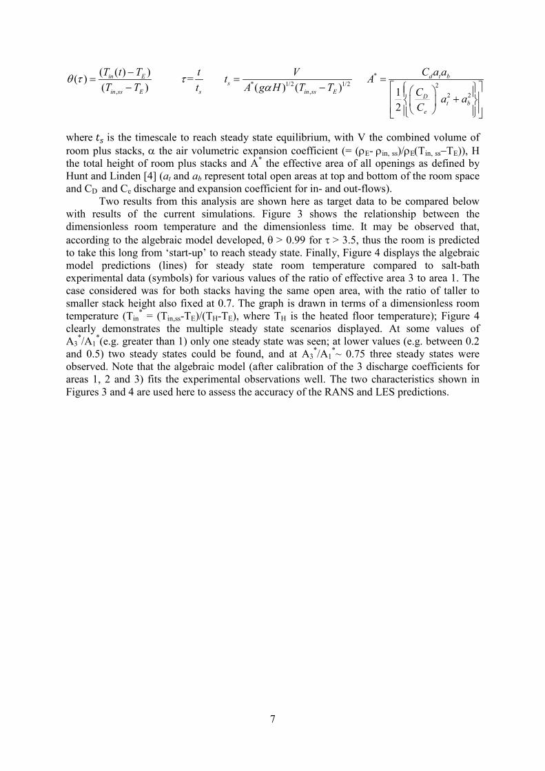
where 𝑡𝑠 is the timescale to reach steady state equilibrium, with V the combined volume of room plus stacks, a the air volumetric expansion coefficient (= (ρE- ρin, ss)/ρE(Τin, ss−ΤE)), H the total height of room plus stacks and A* the effective area of all openings as defined by Hunt and Linden [4] (at and ab represent total open areas at top and bottom of the room space and CD and Ce discharge and expansion coefficient for in- and out-flows).

Two results from this analysis are shown here as target data to be compared below with results of the current simulations. Figure 3 shows the relationship between the dimensionless room temperature and the dimensionless time. It may be observed that, according to the algebraic model developed, θ > 0.99 for t > 3.5, thus the room is predicted to take this long from ‘start-up’ to reach steady state. Finally, Figure 4 displays the algebraic model predictions (lines) for steady state room temperature compared to salt-bath experimental data (symbols) for various values of the ratio of effective area 3 to area 1. The case considered was for both stacks having the same open area, with the ratio of taller to smaller stack height also fixed at 0.7. The graph is drawn in terms of a dimensionless room temperature (Tin

* = (Tin,ss-TE)/(TH-TE), where TH is the heated floor temperature); Figure 4 clearly demonstrates the multiple steady state scenarios displayed. At some values of A3

*/A1*(e.g. greater than 1) only one steady state was seen; at lower values (e.g. between 0.2

and 0.5) two steady states could be found, and at A3*/A1

*~ 0.75 three steady states were observed. Note that the algebraic model (after calibration of the 3 discharge coefficients for areas 1, 2 and 3) fits the experimental observations well. The two characteristics shown in Figures 3 and 4 are used here to assess the accuracy of the RANS and LES predictions.

8

Figure 3: Relationship between dimensionless room temperature and dimensionless time as reported by Chenvidyakarn &

Woods [1]

Figure 4: Comparison between algebraic model predictions and lab experiments. - Steady state temperature vs area of

bottom opening as reported by Chenvidyakarn & Woods [1])

9

3. Mathematical Modelling and Computational Details

3.1. Governing Equations

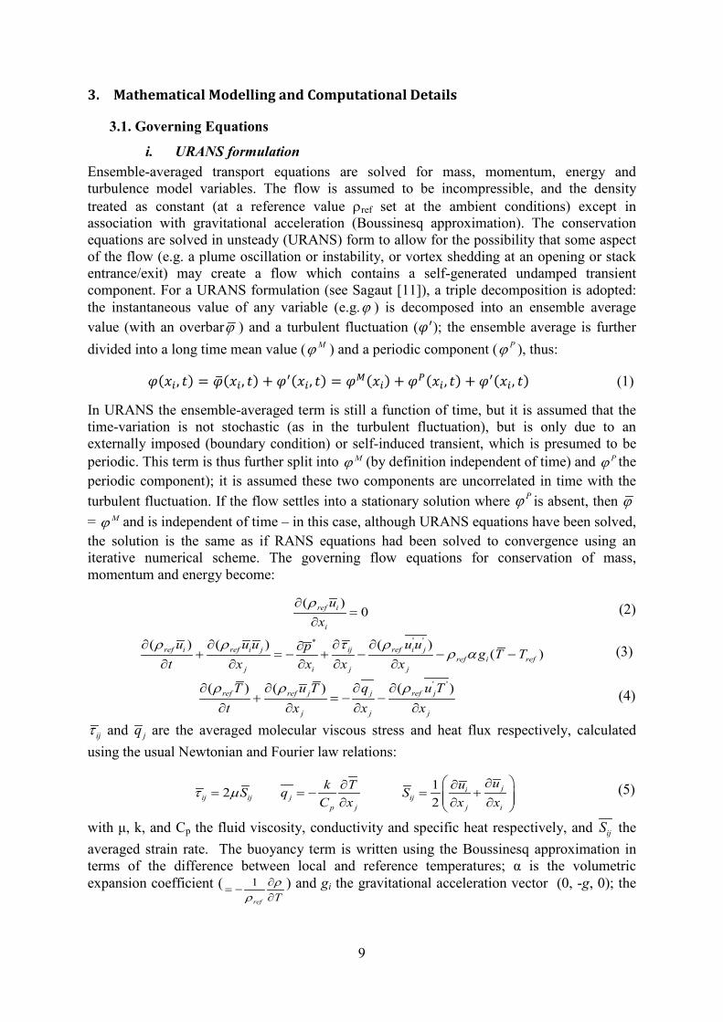
i. URANS formulation Ensemble-averaged transport equations are solved for mass, momentum, energy and turbulence model variables. The flow is assumed to be incompressible, and the density treated as constant (at a reference value ρref set at the ambient conditions) except in association with gravitational acceleration (Boussinesq approximation). The conservation equations are solved in unsteady (URANS) form to allow for the possibility that some aspect of the flow (e.g. a plume oscillation or instability, or vortex shedding at an opening or stack entrance/exit) may create a flow which contains a self-generated undamped transient component. For a URANS formulation (see Sagaut [11]), a triple decomposition is adopted: the instantaneous value of any variable (e.g.ϕ ) is decomposed into an ensemble average value (with an overbarϕ ) and a turbulent fluctuation (𝜑′); the ensemble average is further divided into a long time mean value ( Mϕ ) and a periodic component ( Pϕ ), thus:

𝜑(𝑥𝑖, 𝑡) = 𝜑�(𝑥𝑖, 𝑡) + 𝜑′(𝑥𝑖, 𝑡) = 𝜑𝑀(𝑥𝑖) + 𝜑𝑃(𝑥𝑖, 𝑡) + 𝜑′(𝑥𝑖, 𝑡) (1)

In URANS the ensemble-averaged term is still a function of time, but it is assumed that the time-variation is not stochastic (as in the turbulent fluctuation), but is only due to an externally imposed (boundary condition) or self-induced transient, which is presumed to be periodic. This term is thus further split into Mϕ (by definition independent of time) and Pϕ the periodic component); it is assumed these two components are uncorrelated in time with the turbulent fluctuation. If the flow settles into a stationary solution where Pϕ is absent, then ϕ = Mϕ and is independent of time – in this case, although URANS equations have been solved, the solution is the same as if RANS equations had been solved to convergence using an iterative numerical scheme. The governing flow equations for conservation of mass, momentum and energy become:

( )0ref i

i

ux

ρ∂=

∂ (2)

' '*( ) ( ) ( )

( )ref i ref i j ij ref i jref i ref

j i j j

u u u u up g T Tt x x x x

ρ ρ t ρρ a

∂ ∂ ∂ ∂∂+ = − + − − −

∂ ∂ ∂ ∂ ∂ (3)

' '( ) ( ) ( )ref ref j j ref j

j j j

T u T q u Tt x x x

ρ ρ ρ∂ ∂ ∂ ∂+ = − −

∂ ∂ ∂ ∂ (4)

ijt and jq are the averaged molecular viscous stress and heat flux respectively, calculated using the usual Newtonian and Fourier law relations:

12 2

jiij ij j ij

p j j i

uk T uS q SC x x x

t µ ∂∂ ∂

= = − = + ∂ ∂ ∂ (5)

with μ, k, and Cp the fluid viscosity, conductivity and specific heat respectively, and ijS the averaged strain rate. The buoyancy term is written using the Boussinesq approximation in terms of the difference between local and reference temperatures; α is the volumetric expansion coefficient ( 1

ref Tρ

ρ∂

= −∂

) and gi the gravitational acceleration vector (0, -g, 0); the

10

pressure *p is thus the difference between local mean static pressure and a hydrostatic pressure based on the reference density ( *

ref i ip p g xρ= − )

The turbulent Reynolds stresses ' 'ref i ju uρ and heat fluxes ' '

ref ju Tρ are modelled via an eddy viscosity/diffusivity hypothesis, combined with the k-ε RNG turbulence model (Yakhot et al. [13]) to calculate the eddy viscosity/diffusivity (this model was selected as the review of Chen [9] indicated it was a commonly used eddy viscosity model in ventilation flow applications). Thus the governing equations take the form:

' ' ' '2 -3

ji tref i j t ij ref ref j

j i T j

uu Tu u k u Tx x x

µρ µ δ ρ ρσ

∂∂ ∂− = + − = ∂ ∂ ∂

(6)

,

( ) ( )ref ref i tk b ref

i i k RNG i

k u k k P Pt x x x

ρ ρ µµ ρ eσ

∂ ∂ ∂ ∂+ = − + + + − ∂ ∂ ∂ ∂

(7)

1, 2,

,

( ) ( )( ( ) )ref ref i t

RNG k kb RNGi i RNG i

uC P P C

t x x x k e ee

ρ e ρ e µ e eµ ρeσ

∂ ∂ ∂ ∂+ = + + + − ∂ ∂ ∂ ∂ (8)

2

' ', i

t ref RNG k ref i j kb ref ij i

k u TC P u u P gx xµµ ρ ρ ρ a

e ∂ ∂

= = − = − ∂ ∂ (9)

1, 3

,

(1 )4.381.44 =

(1 )k

RNGRNG ref RNG

PC f fCe µ µ

µ

ηηη

β η ρ e

−= − =

+ (10)

Other turbulence model constants were given their standard values:

, 2, , ,0.085 0.012 1.68 0.7179 0.7179 =0.9 RNG RNG RNG k RNG RNG TC Cµ e eβ σ σ σ= = = = =

ii. LES formulation An LES approach to turbulence closure solves the spatially-filtered Navier–Stokes equations obtained by applying a low-pass spatial filter of characteristic width ∆ to the instantaneous velocity and temperature fields (in the current approach to LES the filter width is taken as proportional to the local cell size so spatial averaging takes place over computational cell volumes, for details see Sagaut [11]); the equations are thus written as follows. NB: in spite of the superficial similarity of the LES equations with (2)-(4) above, the overbar and dashes as defined in eqn. (1) now indicate a spatially-averaged or ‘resolved’ variable, and a ‘residual’ variable respectively:

( )

0ref i

i

ux

ρ∂=

∂ (11)

,*( ) ( ) ( )

( )sgs d

ref i ref i j ij ijref i ref

j i j j

u u u p g T Tt x x x x

ρ ρ t tρ a

∂ ∂ ∂ ∂∂+ = − + − − −

∂ ∂ ∂ ∂ ∂ (12)

( ) ( ) ( )sgs

ref ref j j j

j j j

T u T q qt x x x

ρ ρ∂ ∂ ∂ ∂+ = − −

∂ ∂ ∂ ∂ (13)

11

where *p is now given by * 13

sgsref i i iip p g xρ t= − + and ,sgs d

ijt is the deviatoric part of the sub-

grid-scale (SGS) or residual stress tensor, given by:

, 1

3sgs d sgs sgs

ij ij kk ijt t t δ= − (14)

where: sgsij ref i j ref i ju u u ut ρ ρ= − , and its equivalent in the temperature equation, the SGS

heat flux is: sgsj ref j ref jq u T u Tρ ρ= −

To close this set of equations a model is needed for the SGS stress tensor and heat flux vector. Whilst many alternative and advanced SGS models have been proposed (Sagaut [11]), it is argued here that, as long as the mesh resolution is such that at least ~80% of the fluctuating energy is everywhere captured by the grid (as suggested in Pope [10] and [16] and also by Celik et al. [17]) as representing a well-resolved LES), then the adoption of a simple SGS model is sufficient. One consequence of this requirement is that in near wall regions (where the turbulent eddy size decreases rapidly) an exceedingly fine mesh is needed. It is, however, further argued here that in the present problem it is the free-shear regions associated with in- and out-flowing jets and rising buoyant plumes that determine the important mixing processes, so an approximate treatment of the near wall regions is acceptable. This point is discussed further in the next section where the design of the LES mesh is described. The Smagorinsky SGS model (Smagorinsky [18]) is the simplest SGS model and is written in terms of an eddy viscosity assumption introduced to calculate sgs

ijt . The Smagorinsky model is algebraic and its application in the present problem takes the form:

2 2

,

2 ( ) sgssgs sgsij sgs ij sgs ref ref S j

T sgs j

TS l S C S qx

µt µ µ ρ ρ

σ∂

= − = = ∆ = −∂

(15)

where 1 2

jiij

j i

uuSx x

∂∂= + ∂ ∂

is the filtered strain rate tensor, 1/3( )x y z∆ = ∆ ∆ ∆ (the cube root

of the local cell volume) is the filter length, 1/2(2 )ij ijS S S= is the magnitude of the filtered strain rate tensor, CS denotes the Smagorinsky constant, and ∆x, ∆y and ∆z represent local cell size. Cheng et al. [19] have applied this approach to scalar mixing in jet flows and shown that a simple SGS Prandtl number approach works well ( , 0.7T sgsσ = was used here). One modification that is necessary with this simple model is to introduce extra damping near walls, otherwise the SGS viscosity is large even in low turbulence Reynolds number regions. Thus, the model is modified according to Van Driest [20] via:

2[ (1 exp( )) ]sgs ref SyC SA

µ ρ+

+= − − ∆ (16)

where: CS = 0.1, y+ = ρrefyut/µ, and A+ = 25; ut is the skin friction velocity, y the wall normal distance, and µ the molecular viscosity.

3.2. Computational/Numerical Details

A commercial CFD code, CFX (ANSYS [21]), was utilised for all calculations presented below. This was chosen for convenience in containing a wide range of RANS turbulence models from which to select, and also an LES capability; the availability of a general and flexible mesh generation package (ICEM (CFD)) was also an advantage. The incompressible nature of the flow problem encouraged the selection of a pressure-based solver. The solution domain geometry generated for the CFD analysis was identical to the small-scale model

12

reported by Chenvidyakarn and Woods [1] and is shown in Figure 5, together with the locations of a series of monitor points used to assess the progress of the transient CFD solution. Points P1-P1e were located on the vertical centreline of the enclosure; the first is 5cm from the floor and the 5 others are spaced at 2 cm intervals. P1a-P1e were used to obtain an average internal temperature to compare with measured data. P1-P5 were used to track the progression of the solution from start-up to steady state.

Figure 5: Computational solution domain and monitoring points

For the URANS solutions, predictions on four meshes of different resolution were initially examined on a single test case to establish mesh independency. The criterion used to judge this was the predicted steady state ventilation mass flow rate through the enclosure, assessed by monitoring the stack mass flows at locations P4 and P5 (Figure 5) as well as through the sidewall openings. Meshes of overall sizes 1.0, 1.3, 1.6, and 2.0 million nodes were compared; the predicted mass flow varied by only 0.73% between the last two meshes, and the 1.6 million cell mesh was used for all further URANS predictions (this contained ~36 cells across the smallest sidewall hole (4mm diameter) and ~60 cells for the largest hole (10mm) and ~100 cells across each stack cross-sectional area). For this mesh the dimensionless wall distance y+ had a minimum value of 0.13 and a maximum value of 3.77.

The conventional RANS CFD strategy of continued mesh refinement to establish numerical accuracy is not readily transferable to LES CFD. In addition, it is well known that for LES, the mesh quality is as important as the mesh density - Vanella et al. [22] have shown that a sudden coarsening of the mesh can be very damaging, causing an energy ”pile-up” at the smallest resolved scale in the coarser mesh region. Gant [23] and Celik et al. [17] have developed mesh quality assessment measures for LES, with Benim et al. [24] describing a recent application of the “Index of Resolution Quality” concept of Celik et al. [17]. An

13

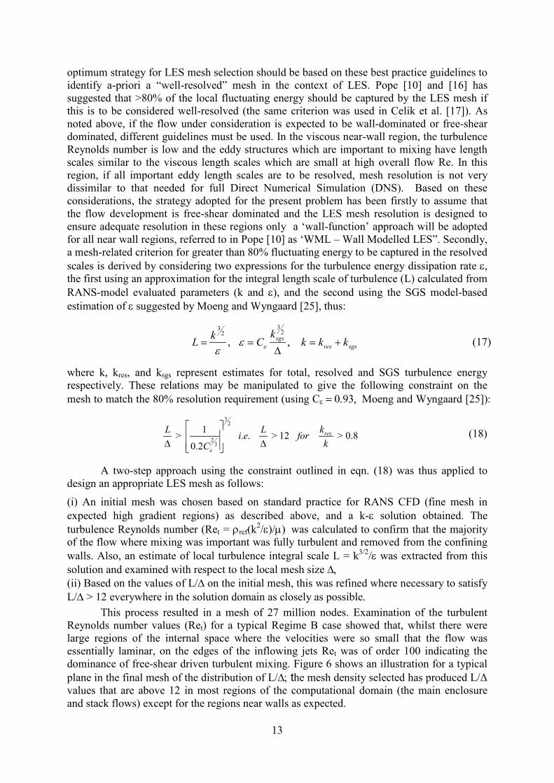
optimum strategy for LES mesh selection should be based on these best practice guidelines to identify a-priori a “well-resolved” mesh in the context of LES. Pope [10] and [16] has suggested that >80% of the local fluctuating energy should be captured by the LES mesh if this is to be considered well-resolved (the same criterion was used in Celik et al. [17]). As noted above, if the flow under consideration is expected to be wall-dominated or free-shear dominated, different guidelines must be used. In the viscous near-wall region, the turbulence Reynolds number is low and the eddy structures which are important to mixing have length scales similar to the viscous length scales which are small at high overall flow Re. In this region, if all important eddy length scales are to be resolved, mesh resolution is not very dissimilar to that needed for full Direct Numerical Simulation (DNS). Based on these considerations, the strategy adopted for the present problem has been firstly to assume that the flow development is free-shear dominated and the LES mesh resolution is designed to ensure adequate resolution in these regions only a ‘wall-function’ approach will be adopted for all near wall regions, referred to in Pope [10] as ‘WML – Wall Modelled LES”. Secondly, a mesh-related criterion for greater than 80% fluctuating energy to be captured in the resolved scales is derived by considering two expressions for the turbulence energy dissipation rate e, the first using an approximation for the integral length scale of turbulence (L) calculated from RANS-model evaluated parameters (k and e), and the second using the SGS model-based estimation of e suggested by Moeng and Wyngaard [25], thus:

33 22

, , sgsres sgs

kkL C k k keee

= = = +∆

(17)

where k, kres, and ksgs represent estimates for total, resolved and SGS turbulence energy respectively. These relations may be manipulated to give the following constraint on the mesh to match the 80% resolution requirement (using Ce = 0.93, Moeng and Wyngaard [25]):

3

2

23

1 > . . > 12 > 0.80.2

resL L ki e forkCe

∆ ∆ (18)

A two-step approach using the constraint outlined in eqn. (18) was thus applied to design an appropriate LES mesh as follows:

(i) An initial mesh was chosen based on standard practice for RANS CFD (fine mesh in expected high gradient regions) as described above, and a k-e solution obtained. The turbulence Reynolds number (Ret = ρref(k2/e)/µ) was calculated to confirm that the majority of the flow where mixing was important was fully turbulent and removed from the confining walls. Also, an estimate of local turbulence integral scale L = k3/2/e was extracted from this solution and examined with respect to the local mesh size ∆, (ii) Based on the values of L/∆ on the initial mesh, this was refined where necessary to satisfy L/∆ > 12 everywhere in the solution domain as closely as possible.

This process resulted in a mesh of 27 million nodes. Examination of the turbulent Reynolds number values (Ret) for a typical Regime B case showed that, whilst there were large regions of the internal space where the velocities were so small that the flow was essentially laminar, on the edges of the inflowing jets Ret was of order 100 indicating the dominance of free-shear driven turbulent mixing. Figure 6 shows an illustration for a typical plane in the final mesh of the distribution of L/∆; the mesh density selected has produced L/Δ values that are above 12 in most regions of the computational domain (the main enclosure and stack flows) except for the regions near walls as expected.

14

Figure 6: L/Δ contours on typical plane for LES predictions

In terms of spatial discretisation, URANS predictions adopted a high resolution convection discretisation scheme, which blends 1st

order upwind and 2nd order central differencing. The

blend factor is automatically varied on the basis of the local solution to achieve the maximum contribution from the 2nd order scheme whilst maintaining stability and boundedness, avoiding over/under-shoots. For LES it is important to use a non-dissipative scheme, and thus a pure 2nd order central difference scheme was selected. Since both URANS and LES formulations involved an unsteady numerical solution, the questions of appropriate numerical treatment of the transient term and the time step must be addressed. For both URANS and LES, a 2nd order backward Euler scheme was used for the transient term. The time-step is best characterised via the maximum Courant-Friedrichs-Lewy (CFL) number anywhere in the mesh (CFLmax = max [u∆t/∆x, v∆t/∆y, w∆t/∆z]). For URANS predictions CFLmax up to as large as 5.0 was found to give adequate resolution of the initial transient. For LES, the time step is set by the requirement to resolve accurately the temporal dynamics of the smallest resolved eddies. Thus, a varying time step was allowed as the flow field developed making sure CFLmax was between the range of 0.5 and 1.0. In physical time units the time step size (∆t) between 20 and 60 milliseconds was typical. Figure 7shows the temperature evolution over time for the three points P1, P2 and P3 (see Figure 5) from a simulation of a Regime B condition. The uniform floor heating and the nature of the Regime B condition (for further details see Section 4) are seen to lead to a nearly constant temperature at these 3 points;

15

approximately 104 time steps are needed for the solution to ‘forget’ its start-up condition, a buffer region of a further 5x103 steps were allowed to be sure a statistically stationary state had been reached, and time-averaging was used to evaluate statistical mean values.

The simulations for this investigation were run on a high performance computer (HPC) which consisted of 161 compute nodes, each having two six-core Intel Xeon X5650 CPUs and 24GB of memory. For URANS simulations eight processors of the HPC were used while for LES 36 processors were utilised. The approximate run time to reach a steady state for URANS was 1 day whilst for LES it was typically take up to 21 days.

Figure 7: LES prediction of time history of instantaneous temperature at 3 monitor points

3.3. Initial and Boundary Conditions

Water at an initial (ambient) temperature of 23oC was used as the working fluid in the simulation (as in the original experiment) with all three components of velocity initially set to zero. A heat input of 90W was uniformly distributed over the floor (all other walls were adiabatic) and initiated at t=0 (again as in the experimental study). For the velocity field, equilibrium log-law-based wall functions were applied at all near-wall cells in both URANS and LES solutions. These wall functions are appropriate when walls can be considered as hydraulically smooth. As near wall flow study was not the focus of this work, the walls were considered smooth. An ‘opening’ boundary condition was imposed at all inlets and outlets, again for both URANS and LES. This allows flow to enter (at ambient temperature) or leave (at the internal node temperature) the domain depending on the current solution-generated pressure field in the vicinity of the opening. For example, if at any instant of time ∆P represents the (positive) difference between ambient pressure (effectively the total pressure for a stagnant ambient) and the local static pressure inside an opening; then Bernoulli’s equation, corrected via a loss coefficient may be used to calculate the velocity component normal to the boundary:

212 ref nP f Uρ∆ =

where f is a loss coefficient (related to discharge coefficient via f = 1/Cd2) and Un is the

normal component of velocity. Cd can vary with Reynolds number and could vary between different openings/stacks (this was part of the calibration process for the algebraic model to

16

fit the experimental data). However, at high Re and for sharp edged openings a discharge coefficient Cd = 0.61 is often taken as standard and this practice was followed here.

3.4.Flow Cases Considered In all calculations the floor heat load and the geometry of the stacks (heights/cross-

sections) were kept constant; only the number and size of openings in the left-hand wall were varied (to reflect experimental practice) to change the value of A3

*/A1*. Chenvidyakarn and

Woods [1] reported that during their experiments the flow always naturally evolved into Regime B (Figure 2b). This was also observed in all calculations (both URANS and LES) conducted here. Irrespective of the value of A3

*/A1* set for the calculation, when the flowfield

was initialised with all components of velocity equal to zero and allowed to progress in time after the heat load was initiated towards a steady state, the Regime B flow pattern with outflow from both stacks was always obtained at steady state. It was known from the measurements that for some values of A3

*/A1* two or more steady state regimes were found

(e.g. for a single 7mm opening all three regimes A, B, and C were possible). To explore if a shift to another regime (A or C) could be ‘triggered’, a technique analogous to that followed in the experiments was adopted. In Regime B upward (outflow) velocities existed at both stacks; to induce a shift from B to A, Chenvidyakarn and Woods [1] had (temporarily) injected fluid downwards in stack 2 (or downwards in stack 1 for a B to C shift). At some A3

*/A1* values the flow had returned gradually to the Regime B condition, but at others the

steady state flowfield had shifted to A (or C); the map in Figure 4 shows the boundaries of which regimes were achievable at different A3

*/A1* values. These observations correspond

well with the ‘strong perturbation’ scenario described by Yuan and Glicksman [8]. A similar procedure was followed in the present CFD study. For example, from a steady state Regime B solution and to investigate a possible shift to Regime A, the boundary condition at the shorter stack exit was temporarily changed from ‘opening’ to ‘inlet’ with a reversed velocity boundary condition at the same magnitude that existed in the steady state B solution. The simulation was re-started and after 30s the ‘inlet’ boundary condition was changed back to an ‘opening’ type boundary condition, thus allowing the flow to evolve unconstrained until stability was achieved. It was observed that, as in the experiments, for some A3

*/A1* values

the flow reverted back to the B condition, and for others it settled stably into steady state A. A similar procedure was followed to explore B to C changes. In this way a predicted ‘steady state regime map’ could be established for the CFD (either URANS or LES).

4. Results

4.1.Start-up to Steady State

A statistically stationary state was considered to have been reached when information from the various monitoring points (Figure 5) indicated that the following criteria had been met:

• Time-mean ventilation flows through the stack outlets (P4, P5) and the inflow through the lower sidewall openings were unchanging with time. An example of this is shown in Figure 8 for a URANS prediction of a Regime B flow case; the ventilation flows through the lower openings and stack outlets converge to steady values and the transient changes in mass flow stabilise after about 5000 time steps.

• Time-mean velocity, temperature and pressure values at monitor points P1, P2, P3 were stable (an example for an LES prediction is shown in Figure 7).

Note: it is necessary to time-average the LES solution (once it has reached a statistically stationary state, see Figure 8) since this constantly varies in time at all points. As noted above,

17

in following a URANS formulation and solution, this allows for a time-varying solution containing a self-induced periodic velocity field ( P

iu ) and hence a time-varying predicted ensemble-average ( iu ). It was observed, however, under all flow conditions explored, that the periodic component was zero and the solution settled into a non-time-varying state (i.e.

( )iu f t≠ ). In this sense the solutions obtained are more correctly labelled below as RANS rather than URANS solutions. Given the large scale unsteadiness seen in the LES solutions, the most likely explanation for this is that any tendency for the URANS solution to generate a time-varying component was damped out by the high level of eddy viscosity produced by the RNG k-e turbulence model; whether any other model would have allowed any self-induced unsteadiness is at present not clear.

Figure 8: Flow through lower openings (top), short stack (middle), tall stack (bottom)

Figure 9 shows (for a Regime B case) the evolution of the predicted average room temperature (Tin) with time for both RANS and LES and also the level of steady state temperature from the algebraic model theory developed by Chenvidyakarn and Woods [1]. The characteristic room temperature was extracted by taking a mean of the temperature at the

18

monitor points P1a to P1e in accordance with a similar technique adopted in the experiment. It can be seen that both RANS and LES predict a similar time-history during the initial transient, although different steady state temperatures are achieved. The LES prediction is noticeably closer to the algebraic model predictions (which were fitted to the experimental data). Both RANS and LES show the room to reach steady state in 1.6 hours; this corresponds to a non-dimensional time t = 3.505 which compares favourably to the time to converge to equilibrium of t = 3.5 noted in the measurements.

Figure 9: Comparison of time for Tin to reach steady state using RANS, LES and algebraic model of Chenvidyakarn and

Woods [1] (shown by dotted line)

4.2.Multiple Steady States

Considering the case of a single opening of 7cm diameter in the left hand wall, Figure 10 shows the RANS model was able to predict a stable solution in all three regimes. Temperature plots in a vertical plane midway through the domain and passing through both the lower opening centre and the two stack centres are displayed. The direction of flow through the stacks in each regime can easily be identified from the stack fluid temperature, with cold ambient air implying inflow and warm mixed air implying outflow. Ambient air flows in through the lower sidewall opening in all three regimes, but its penetration distance across the space is very different in each regime. The furthest penetration is in Regime B, where it reaches almost halfway across before mixing rapidly and being heated by the floor heat load; in this regime, the whole region below the inflow height (apart from a small zone in the lower left corner) is filled with relatively cool air. In Regime A the down-flow from the smaller stack impinging on the floor provides an obstruction to the inflowing ambient air, which thus penetrates slightly less than in Regime B before it is deflected upwards and off the vertical plane plotted. In Regime C the taller stack down-flow impinges directly onto the ambient inflow and pushes this down towards the floor, causing the smallest cross flow penetration into the domain amongst the three regimes. According to the algebraic model [1] the internal space should be well mixed and thermally uniform. In contrast, the RANS temperature plots suggest the internal space contains three stratified regions; a lower region containing both cold and mixed fluid, a central region comprising about 70% of the volume

23

24

25

26

27

28

29

30

31

32

33

0 1000 2000 3000 4000 5000 6000 7000 8000

Room

tem

pera

ture

(o C)

Time (s)

URANS LES

19

that is well mixed, and an upper region with warmer air above that might be identified (at ~80% height) as an internal temperature interface above a vertical temperature gradient (albeit only a small gradient). Regime A produces small regions of hottest air near the right hand wall, Regime B has similar regions both below and above the inflowing ambient air, but in Regime C the hottest air is in the bottom right hand corner, presumably caused by a long residence time of air that has flowed across the floor being heated during its passage before turning upwards at the right hand wall.

Figure 10: RANS temperature predictions on a plane midway through the domain (a) Regime A, (b) Regime B and (c)

Regime C

The RANS-predicted temperature mixing that can be seen in Figure 10 can be understood clearly if the turbulence energy (non-dimensionalised by the inflowing ambient air velocity through the lower opening in each regime i.e. k/Uin

2) contours in Figure 11 are examined. These plots underline the point made earlier that quite large regions of the internal space are filled with essentially laminar flow and hence little mixing occurs in these regions. The high rates of cold/warm air mixing are concentrated on the edges of the inflowing air jets in each regime as illustrated by the high levels of turbulence energy shown in Figure 11.

20

Figure 11: Turbulence energy contours in the three flow regimes (non-dimensionalised by the inflowing ambient air velocity

in each regime)

The steady RANS temperature contours in Figure 10 may be compared and contrasted with the samples provided in Figure 12 at three time instances taken from LES predictions for the same geometry at the Regime A, B, and C conditions. Regime B has the closest similarity between LES and RANS; the primary difference is that in the LES solution the cross-room penetration of the cold inflowing ambient plume can be seen to vary in time; accompanying this is a time varying vertical depth of the right hand mixed portion of this plume, which also never achieves quite the same level of mixing as in the RANS prediction, indicating a portion of ambient temperature air penetrates across the full width of the room at all three time instances shown. In regime A the inflowing cold plume from the stack displays a remarkably small level of mixing, much smaller than in the RANS prediction before it impinges on the floor; also its trajectory is vertical, whereas the RANS plume deviates slightly towards the right wall. The explanation for this low level of mixing is that the down-flowing plume is surrounded by down-flowing mixed warm air created by the general recirculation induced in the room (see Figure 13), so that the level of shear at the plume interface is small. As a result, the ambient cross-room wall jet after it has reached floor level, displays a very unsteady behaviour in close proximity to the vertical down-flowing plume and gets deflected upwards. In stark contrast to Regime A, in Regime C the inflowing stack plume is much more turbulent, deviates away from rather than towards the left wall as in the RANS solution, and breaks down into large eddy structures before they reach the mid-height of the domain. The much larger rate of mixing and the violent behaviour of the large scale turbulent structures are caused because in this case the down-flowing plume is opposed by the warm air updraft on the left-hand wall, increasing the rate of shear greatly.

21

Figure 12: LES temperature predictions on a vertical plane midway through the domain for Regimes A, B, and C and at (a)

time = tss-10sec, (b) time = tss, and (c) time = tss+10sec

22

Figure 13: Vector plot for Regime A at time = tss showing down-flowing plume surrounded by down-flowing fluid produced

by general recirculation induced in the room (vectors are normalized to make them the same size)

Figure 14 illustrates the process of a switch from regime C to Regime B induced by the stack boundary condition changes described above. Instantaneous temperature contours and velocity vectors throughout the room space and stacks are shown. Figure 13a indicates an instantaneous snapshot characteristic of the statistically stationary state for Regime C, with down-flow/up-flow in the taller/shorter stack respectively. The violent nature of the opposed flows (down-flowing cold ambient air and up-flowing warm mixed air) against the left-hand wall is illustrated very well via the velocity vectors and explains the ‘billowing’ nature of the buoyant plume and the large scale turbulent eddies generated.

Figure 14b illustrates the flow conditions 190 seconds after the switch in boundary condition has taken place at the taller stack. Note, the boundary condition switch was only ‘forced’ for 30 seconds; subsequently the flow solution is allowed to find its own direction of the stack entry velocity. The strong down-flowing plume has disappeared and this has also enabled the inflowing ambient air to penetrate further across the room; the associated reduced mixing means that a zone of warmer air has begun to grow near to the room ceiling. Ingress of warm air into the taller stack has just begun near the stack right hand wall. The continuation of the flow development is shown in Figure 14a; the situation a further 8 seconds after Figure 13b indicates that the warm air ingress continues, as does the penetration of the ambient wall-jet across the floor and the growth of the ceiling warm air zone. Gradually the warm air continues to fill the entire tall stack volume and up-flow on the left hand wall and down-flow on the right hand wall begin to dominate the flow pattern in the

23

internal space. A snapshot characteristic of the final statistically stationary solution for Regime B (after a further 105 seconds has elapsed after Figure 14a) is shown in Figure 14b.

Figure 14: Instantaneous LES temperature and velocity vector predictions during the switch from regime C to regime B:

(a) t = tss,C (b) t = tss,C+190s

24

Figure 15: Instantaneous LES temperature and velocity contour predictions during the switch from regime C to regime B:

(a) t = tss,C+198s (b) t = tss,C+198s = tss,B

25

Finally, when the solutions provided by the RANS/LES methods for the whole range of A*

3/A*1 are assembled, it is possible to plot similar regime maps for each solution

methodology as done for the experiments by Chenvidyakarn and Woods [1]. Figure 16 provides these for RANS (left) and LES (right) (note that in Figure 16 it is the algebraic model predictions of Chenvidyakarn and Woods [1] that are included rather than the raw measurements, since the model fitted the experimental data very closely. The figures show

dimensionless temperature * ,,

( )( )

in ss Ein ss

H E

T TT

T T−

=−

, where TH is the temperature of the heat source.

In general it may again be noted that both modelling approaches capture the three regime nature of the problem. However, in several areas the LES predictions display better agreement with the fitted experimental data curves. For example, at larger doorway areas (large * *

3 1/A A ), where Regime B dominates, RANS under-predicts the room temperature compared to LES. Similarly RANS predictions become inadequate for * *

3 1/A A < 1.0. Although RANS does predict the existence of Regimes A and C, it does not distinguish the measured temperature difference between the two states, also the dimensionless room temperature is under-predicted for regime B and over-predicted for regimes A and C, due to RANS predicting less mixing of the incoming cool air. LES appears to be more accurate throughout the range of opening areas explored, showing very close agreement with the algebraic model.

5. Conclusions Multiple steady states in buoyancy-driven natural ventilation have been investigated using both LES and URANS CFD methodologies. The theoretical model fitted to the experimental data implied that the average room temperature of the enclosure was 31.60oC. LES predicted an average temperature of 31.65oC (0.15% discrepancy) and URANS predicted 32.05oC (a 3-fold larger discrepancy). LES was however 4.5 times expensive in terms of computational power and 21 times in terms of time. This does highlight the limitation of LES to compete with URANS in terms of its application for real buildings with more complex geometries (see for example Durrani [26]).

Figure 16: CFD predictions (symbols – RANS (left), LES (right)) for regime map ( *,in ssT vs * *

3 1/A A ) compared to

Chenvidyakarn and Woods [1] algebraic model (dotted lines)

26

The relationship between the dimensionless room temperature 𝜃, and the dimensionless time to converge to equilibrium, 𝜏, was also predicted. According to theory, when 𝜏 > 3.5, then θ ~ 1. This was predicted well by both modelling techniques although LES proved again to be more accurate than URANS.

It was identified that, for an area ratio of 0.8 (i.e. the area of the doorway relative to the cross-sectional area of the stacks), three steady state regimes were predicted by both LES and URANS in line with experimental observations. The URANS method, however, was unable to capture any detail of the flow structures observed in the measurements or maintain any continuing unsteadiness, in all cases converging onto a permanent steady state. These deficiencies were removed in the LES solution. This is perhaps an expected consequence of the damping inherently introduced by the eddy viscosity of the URANS method. URANS also predicted a weak vertical temperature gradient in the domain which was not observed in the experimental work where a well-mixed environment was predicted. This feature was correctly captured by LES, which predicted the flow to comprise recirculating convection currents in the region where URANS had predicted a vertical temperature gradient.

Differences between LES and URANS performance in predicting the multiple steady state regimes for all values of the bottom opening area ratio and the respective room temperatures were investigated. It was observed that URANS did not perform well in predicting the room temperatures for area ratios less than 0.5. URANS over-predicted the temperatures, especially for Regime A. LES on the other hand performed well for all area ratios. This difference is undoubtedly due to differences in the large scale mixing predicted by the two modelling approaches. LES predictions showed a different mixing pattern within the enclosure than URANS. By its nature, LES requires considerably more computing power than URANS. However, in the present work, aided by the method used to define an optimum energy capturing LES mesh, the LES solutions required only approximately five times more time than URANS (using the same hardware platform).

In conclusion it was found that even though LES is more computationally expensive and does not necessarily have a major advantage over URANS in predicting average room temperature, it was however more successful than URANS in predicting the multiple steady states and both qualitative and quantitative flow phenomena for natural ventilation in the geometry investigated.

6. Acknowledgements This paper uses the experimental data reported by Chenvidyakarn and Woods [1]. The authors would like to thank Dr Torwong Chenvidyakarn for discussions on the experiments undertaken.

7. References 1. Chenvidyakarn, T. and A. Woods, Multiple steady states in stack ventilation. Building

and Environment, 2005. 40(3): p. 399-410. 2. DTLR, The Building Regulations 2000, Convservation of Fuel and Power. The

Stationery Office, 2000. 3. Linden, P.F., The Fluid Mechanics of Natural Ventilation. Annual Rev. Fluid Mech,

1999. 31: p. 208-238.

27

4. Hunt, G.R. and P.F. Linden, Steady-state flows in an enclosure ventilated by buoyancy forces assisted by wind. Journal of Fluid Mechanics, 2001(426): p. 355-386.

5. Li, Y., et al., Some examples of solution multiplicity in natural ventilation. Building and Environment, 2001. 36(7): p. 851-858.

6. Yuan, J. and L.R. Glicksman, Transitions between the multiple steady states in a natural ventilation system with combined buoyancy and wind driven flows. Building and Environment, 2007. 42(10): p. 3500-3516.

7. Andersen, K.T., Airflow rates by combined natural ventilation with opposing wind—unambiguous solutions for practical use. Building and Environment, 2007. 42(2): p. 534-542.

8. Yuan, J. and L.R. Glicksman, Multiple steady states in combined buoyancy and wind driven natural ventilation: The conditions for multiple solutions and the critical point for initial conditions. Building and Environment, 2008. 43(1): p. 62-69.

9. Chen, Q., Ventilation performance prediction for buildings: A method overview and recent applications. Building and Environment, 2009. 44(4): p. 848-858.

10. Pope, S.B., Turbulent Flows. Cambridge University Press, 2000. 11. Sagaut, P., "Large Eddy Simulation for incompressible flows: an introduction". 2nd

Edition ed. 2006: Springer. 12. Launder, B.E. and D.B. Spalding, The numerical computation of turbulent flows.

Computer Methods in Applied Mechanics and Engineering, 1974. 3: p. 269-289. 13. Yakhot, V., et al., Development of turbulence models for shear flows by a double

expansion technique. Physics of Fluids A, 1992. 4(7): p. 1510-1520. 14. Durrani, F., et al., Large Eddy Simulation of buoyancy-driven natural ventilation -

Twin-plume flow. International Journal of Ventilation, 2013. 11(4): p. 353-366. 15. Heiselberg, P., et al., Experimental and CFD evidence of multiple solutions in a

naturally ventilated building. Indoor Air 2004(14): p. 43-54. 16. Pope, S.B., Ten questions cencerning the large-eddy simulation of turbulent flows.

New Journal of Physics, 2004. 6. 17. Celik, I.B., Z.N. Cehreli, and I. Yavuz, Index of resolution quality for large eddy

simulations. Journal of fluids engineering, 2005. 127: p. 949-958 18. Smagorinsky, J., General circulation experiments with the primitive equations.

Monthly Weather Review, 1963. 91(3): p. 99-164. 19. Cheng, L., et al., Validation of LES predictions of scalar mixing in high swirl fuel

injector flows. Flow Turbulence and Combustion, 2012(88): p. 146-168. 20. Van Driest, E.R., On turbulent flow near a wall. J. Aerosol Sci, 1956(23): p. 1007–

1011. 21. ANSYS, ANSYS CFX-Modelling Guide. ANSYS CFX Documentation, 2011. 22. Vanella, M., U. Piomelli, and E. Balaras, Effect of grid discontinuities on large-eddy

simulation statistics and flow fields. Journal of Turbulence, 2008: p. N32. 23. Gant, S., Reliability Issues of LES-Related Approaches in an Industrial Context. Flow,

Turbulence and Combustion, 2010. 84(2): p. 325-335. 24. Benim, A.C., et al., Analysis of turbulent swirling flow in an isothermal gas turbine

combustor model, in ASMe Turbo Expo Conf. 2014: Duesseldorf, Germany. 25. Moeng, C.H. and J.C. Wyngaard, Spectral analysis of LES models of the convective

boundary layer. Jnl. Of the Atmos. Sci., 1988(45): p. 3573-3587. 26. Durrani, F., Using Large Eddy Simulation to Model Buoyancy-Driven Natural

Ventilation, in School of Civil and Building Engineering. 2013, Loughborough University: Loughborough.