evaluation of liquefaction potential of impounded class f
TRANSCRIPT
Evaluation of Liquefaction Potential of Impounded
Class F Fly Ash
Thesis Write-Up
The Ohio State University Research Project # 60024835
December 2009 - March 2013
Submitted to: The Ohio State University Knowledge Bank
Department of Civil and Environmental Engineering and Geodetic Science
The Ohio State University
470 Hitchcock Hall, 2070 Neil Avenue
Columbus, Ohio 43210
March 22, 2013

i
Abstract
The purpose of this study was to evaluate the liquefaction potential of impounded Class F fly ash
and compare the results to a 2005 study at the Ohio State University by Zand et al. A computer
ground response analysis program, SHAKE, was used to obtain the cyclic stress ratios and
equivalent number of cycles during several variations of a design earthquake. The profiles are
based upon an actual impounded fly ash unit at an American Electric Power (AEP) plant. Cyclic
triaxial tests were also performed on reconstituted specimens. The tests were performed at
varying cyclic stress ratios, sample densities, and confining stresses. The results of the computer
analyses were compared with laboratory testing which found the design seismic loading to be
lower than the cyclic strength of the fly ash. This result is consistent with the 2005 study;
however, the correlation between confining stress and liquefaction potential was not.
Acknowledgements
I would like to thank my research advisors, Dr. William Wolfe and Dr. Tarunjit Butalia for all
their support and guidance over the past three years. I would also like to thank Nathan Yencho
and Brian Dudley for their work during laboratory testing. Their hard work was invaluable to this
project.

ii
Table of Contents Abstract .......................................................................................................................................................... i
Acknowledgements ........................................................................................................................................ i
List of Figures and Tables............................................................................................................................ iii
List of Equations .......................................................................................................................................... iii
Chapter 1 Introduction .................................................................................................................................. 1
1.1 Motivation ..................................................................................................................................... 1
Chapter 2 Methodology ................................................................................................................................ 3
2.1 Laboratory Tests ................................................................................................................................. 3
2.1.1 Sample Preparation ...................................................................................................................... 3
2.1.2 Specimen Preparation .................................................................................................................. 4
2.1.3 Cyclic Test ................................................................................................................................... 4
2.2 Computer Modeling ............................................................................................................................ 5
2.2.1 Soil Profile Inputs ........................................................................................................................ 6
2.2.2 Soil Profile Analysis .................................................................................................................... 7
Chapter 3 Results and Discussion ................................................................................................................. 8
3.1 Cyclic Test Results ............................................................................................................................. 8
3.2 Computer Model Results .................................................................................................................. 11
Chapter 4 Summary and Conclusion .......................................................................................................... 19
4.1 Summary ........................................................................................................................................... 19
4.2 Conclusions ....................................................................................................................................... 19
List of References ....................................................................................................................................... 21
Appendix A: Laboratory Test Results ........................................................................................................ 23
Appendix B: Ground Response Analysis Results ....................................................................................... 47

iii
List of Figures and Tables
Figure 2.1: Visual definition of the Liquefaction …..………………………………………1
Table 3.1: Cyclic Test Results ……………………………………………………………..4
Table 3.2: Site Characteristics of Profile KK-1 …………………………………………….4
Table 3.3 Site Characteristics of Profile KK-2 ……………………………………………..4
Table 3.4: Computer Model Results Analysis ……………………………………………...4
Figure 3.1: Plotted Liquefaction Results …………………………………………………...4
Figure 3.2: Soil Profile KK-1 ………………………………………………………………4
Figure 3.3: Soil Profile KK-2 ………………………………………………………………4
Figure 3.4: Combined Results of Laboratory Tests and Computer Models ……………….4
List of Equations
Equation 2.1: Cyclic Stress Ratio …………………………………………………………1
Equation 3.1: Maximum Shear Modulus and Shear Wave Velocity ……………………..4
Equation 3.2: Cyclic Shear Stress Amplitude to Maximum Shear Stress Amplitude ….....4
Equation 3.3: Field Cyclic Stress Ratio to Laboratory Cyclic Stress Ratio ………………4
1
Chapter 1 Introduction
1.1 Motivation
In 2011, approximately 60 million tons of fly ash was produced in the United States alone. Of
this total, 38% was reused and the remainder left in landfills or storage ponds (AACA 2013).
When designing these containment areas, liquefaction potential during seismic events is a key
piece of knowledge. Liquefaction of soils can cause severe and costly structural damage.
Combining this fact with environmental hazards associated with industrial by-products such as
fly ash, understanding the liquefaction potential of soil-like materials becomes hyper critical.
By the mid-1970’s, many studies on the liquefaction characteristics of sand and clay had been
completed. Seed et al (1975-1) completed a study to determine the effects of small versus large
scale testing on the liquefaction resistance of sand. Previous studies had already suggested that
intact and reconstituted specimens typically have different soil structures which can have a
significant effect on liquefaction resistance. Typically, intact specimen test results are more
accurate to in-field results; however, obtaining these specimens and maintaining their in-situ
characteristics is difficult. Although yielding different results, Seed et al developed correlations
to normalize random earthquake data and relate them to response data obtained on reconstituted
laboratory specimens. Seed et al (1970) compiled the results of many ground response analyses
to provide a guide for selecting the dynamic shear moduli and the damping ratios. This data
compilation aided in the selection of the dynamic shear moduli and damping ratios for this study.
Because fly ash is a non-plastic material like sands, much of the testing protocol is based upon

2
equations and conclusions developed for sand. Also, the moduli and ratios for fly ash were
based on those for sand.
Limited liquefaction potential testing has been performed on Class F fly ash. In 2005, a study
completed at the Ohio State University sought to expand the available information. The objective
of the study was to evaluate the liquefaction potential of fly ash from an American Electric
Power plant (Zand et al. 2005). The study combined cyclic triaxial laboratory testing with
computer simulation through SHAKE software to determine the threat an earthquake would
impose on a fly ash storage pond. The study resulted in a strong correlation between the onset of
liquefaction and initial dry density of specimen and a weaker correlation between the onset of
liquefaction and confining stress.
The purpose of this project was to evaluate the liquefaction potential of fly ash from a different
American Electric Power facility and follow similar methodology to the 2005 study. This will
establish whether or not the correlations between liquefaction and different fly ash characteristics
apply to different types of fly ash.

3
Chapter 2 Methodology
All laboratory tests and numerical modeling was carried out in the Soil Mechanics Laboratory of
the Department of Civil and Environmental Engineering and Geodetic Science at The Ohio State
University
2.1 Laboratory Tests
Laboratory testing consisted of creating reconstituted Class F fly ash specimens, saturating the
specimens, and testing the specimens under various cyclic stress ratios.
2.1.1 Sample Preparation
Reconstituted Class F fly ash specimens were prepared from a fly ash sample provided by
American Electric Power because intact specimens could not be recovered. A wet depositional
method was used to simulate how fly ash is stored in the field. 500 g of oven-dried fly ash was
weighed and placed in a mixing bowl. Distilled water was added to the ash and mixed until a
paste was formed. The paste was fluviated into large triaxial chamber in layers to create a bulk
sample. Typically, five, 500 g layers were used to make a sample. Layers were scarified with a
spatula to ensure bonding between layers. After placing the last layer, the triaxial chamber was
fully assembled with the addition of a circular plate which rested on top of the sample. The initial
height of the sample was measured and noted.
The bulk sample was left to cure for 24 hours. After the cure period, samples were either
consolidated under a 71.55 psi stress or not consolidated at all. This was done to determine how
density affected liquefaction potential. If the sample was consolidated, a final sample height was
measured.

4
2.1.2 Specimen Preparation
After the sample was fully prepared and cured, the top of the triaxial chamber was removed.
Four copper pipe segments approximately 3-1/2 inches in length and 1-1/2 inches in diameter
were inserted into the top of the sample. A PVC pipe segment of similar dimensions was also
inserted into the top of the sample. The copper pipe molds provided stability for and prevented
damage of specimens when installing them into the triaxial cell. The PVC pipe mold had a
thinner wall thickness which allowed it to fit in the same bulk sample with four copper molds.
After the molds were fully inserted into the top of the bulk sample, the cell was carefully
removed to expose the bulk sample. A moisture content sample was removed from the bulk
sample, weighed and placed in an oven with a temperature of 40˚C to 45˚C. The specimen in the
PVC extruder was removed, weighed, and placed in the same oven as measure of dry density and
moisture content. Each copper tube specimen was removed from the sample. The ends of each
specimen were smoothed with excess portions of the bulk sample. The specimens were weighed
and installed in a triaxial chamber with a surrounding membrane. The installed specimens were
then attached to a pressure panel. A pressure gradient was established with slightly higher
pressure on the bottom of the specimen than the top. This was done to saturate the specimen.
2.1.3 Cyclic Test
Specimens were left to saturate for at least 24 hours. The degree of saturation was judged by the
measure B-value. The B-value is found by measuring the pore pressure differential when the cell
pressure was increased. The pore pressure differential is then divided by the increased cell
pressure. Once the B-value reached at least 95% or two weeks of saturation had occurred, the
specimen was secured in a MTS hydraulic load frame controlled by an MTS Test Star Controller.
An effective confining stress of approximately 20 or 40 psi was applied to the specimen.

5
The MTS machine applied a specified cyclic loading which was measured with a 200 lb
capacity load cell. The loading was derived from the selected cyclic stress ratio (CSR). The CSR
is defined as follows (Kramer, 1996):
(2.1)
is the applied cyclic stress, and is the effective confining stress.
Pore pressure was measured with a Honeywell 100 psig capacity pressure transducer. The pore
pressure measurements are used to determine when liquefaction occurs which is detailed in the
next chapter. Displacement was measured with the internal linear variable differential
transformer (LVTD) of the MTS load frame.
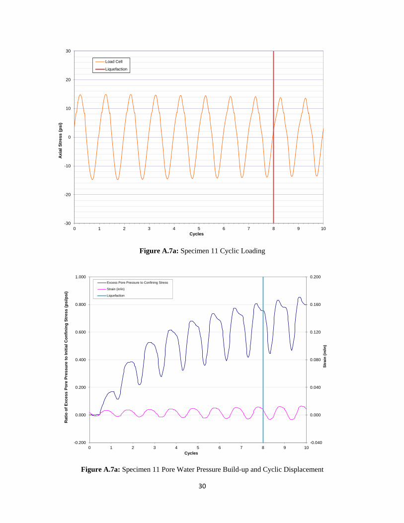
The onset of liquefaction was defined as the point at which the excess pore pressure was
equivalent to the initial confining stress or the point at which the axial stress readings were no
longer equal to or greater than 95% of the programmed load. Whichever event occur first
defined the onset of liquefaction. The criteria coupled with a significant increase in strain
amplitude completed the definition. An example of the onset of liquefaction can be found in
Figure 2.1 below. All tests were performed until either the onset of liquefaction or 500 loading
cycles had occurred.
2.2 Computer Modeling
The computer modeling used a program called SHAKE. This program is a one-dimensional
wave propagation, earthquake analysis program. Several soil profiles and inputs were created
and analyzed using this program.

6
Figure 2.1: Visual definition of the Liquefaction
2.2.1 Soil Profile Inputs
To begin the modeling process, a private communication with AEP provided a previous study to
be analyzed. The study used a two-dimensional modeling program known as QUAKE to study
several soil profiles. Both this project and the AEP study are of the same fly ash pond.
Two, one-dimensional profiles were created in SHAKE based upon one of the two-dimensional
profiles provided in the private communication. The profiles were selected based on vicinity to
the original and current dikes which are considered critical structures. Also, each of the created
profiles has a different total thickness of fly ash. The profile characteristics including layer
thickness, unit weight, water table level, and the small strain shear modulus were provided by the
AEP private communication.
7
The modulus reduction curve and damping curve were selected based upon the soil description
from the AEP private communication and the available data from Seed et al (1970). These curves
are meant to relate shear strain amplitude to shear moduli and damping ratio respectively. When
differences in material description from the original OSU study occurred, curves were selected
based upon the following principles ("EduPro Civil Systems, Inc.").
1. The modulus reduction curve is a measure of how non-linear a soil’s stress-strain
relationship is. A decrease in the plasticity index will increase the non-linear
behavior.
2. The damping curve is a measure of how oscillations in a system will decay with
variation in the shear strain. A decrease in plasticity index will increase soil damping.
Two input earthquake motions were selected for these models: the El Centro earthquake and the
Taft earthquake. Because the ground acceleration amplitude of these earthquakes is much larger
than the predicted amplitudes in the area of the power plant, the ground acceleration was scaled
down to 0.08g or 0.15 g. Similar decisions were made for the previous OSU study.
2.2.2 Soil Profile Analysis
After applying the input motion to the soil profiles, results graphs were selected from the output
module. A table containing the peak stress values in the center of each layer of interest was
compared with the normalized stress time history of that layer. The details of this analysis will be
explained in the chapter 3.

8
Chapter 3 Results and Discussion
The cyclic test results are presented in Appendix A. The detailed computer model analyses
results can be found in Appendix B. A summary and discussion of results of the ground response
analysis and laboratory tests are presented in this chapter.
3.1 Cyclic Test Results
Table 3.1 contains the tabulated results of the cyclic tests. These results are plotted in Figure 3.1
according to the number of cycles to liquefaction and the cyclic stress ratio. The data are
separated by confining stress. Based upon these results, upper and lower results bounds were
established. A red dashed lined marks the 500 cycle test limit at which a specimen was
considered not liquefied.

9
Table 3.1: Cyclic Test Results
DNL = Did not liquefy within 500 cycles.

10
Figure 3.1: Plotted Liquefaction Result
0
0.05
0.1
0.15
0.2
0.25
0.3
0.35
0.4
0.45
1 10 100 1000
Cyc
lic S
tre
ss R
atio
(C
SR)
Cycles to Liquefaction
Sporn Fly Ash Confining stress= 20 psi
Sporn Fly Ash ConfiningPressure = 40 psi
Did not liquefy at 500 cycles.
Class F Fly Ash, 20 psi effective confining stress Class F Fly Ash, 40 psi effective confining stress
11
3.2 Computer Model Results
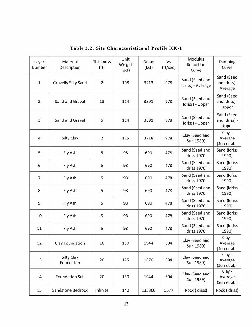
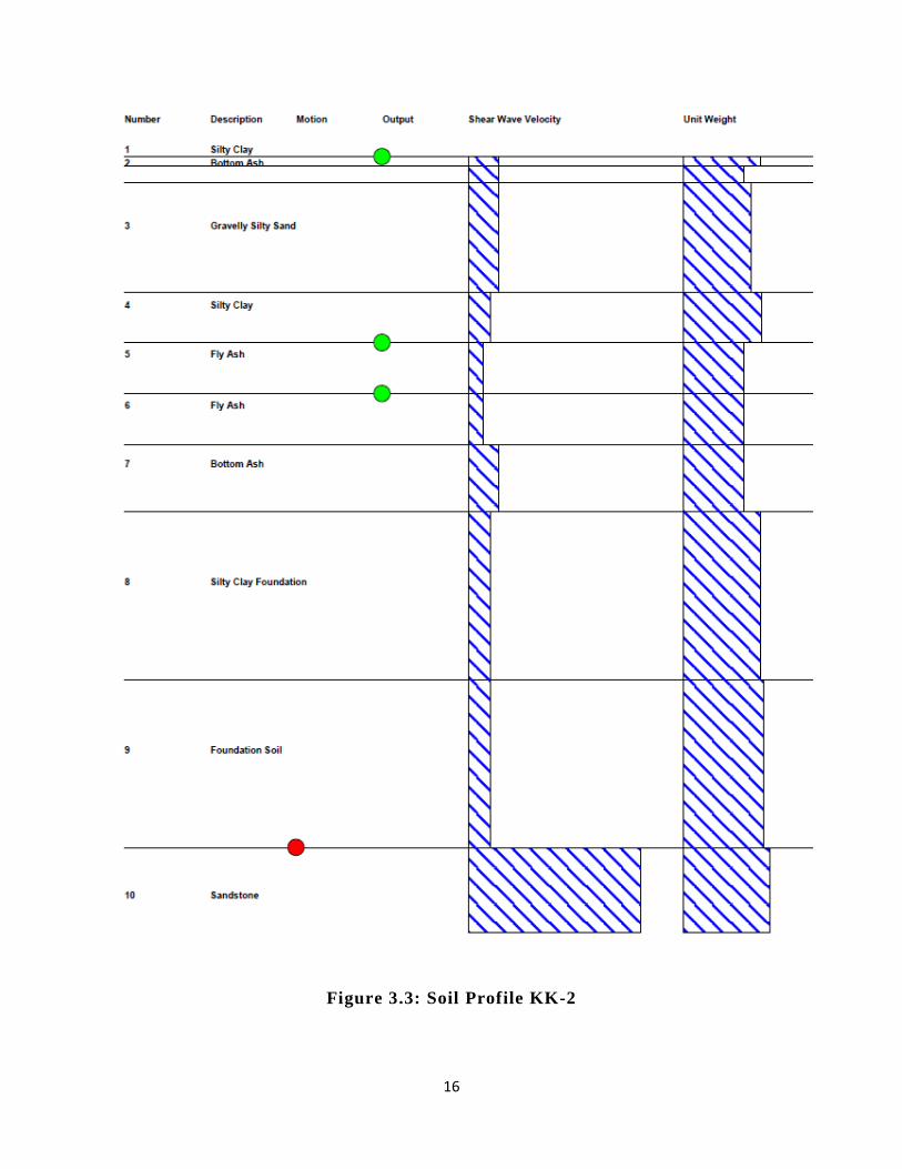
Tables 3.2 and 3.3 detail the site characteristics of profile KK-1 and KK-2 respectively. Figures
3.2 and 3.3 below are illustrations of profiles KK-1 and KK-2. The profiles show relative profile
thickness, soil descriptions, location of motion application, output motion measurement
locations, relative shear wave velocity, and relative unit weight. The red dots indicate where the
earthquake motion was applied. The green dots show where the output motions were analyzed.
Amplitude of the ground motion depends on the shear modulus (G) or shear wave velocity (Vs).
Measurements of the maximum shear modulus were provided by the ground motion analysis
done by AEP in the two-dimensional software, QUAKE. These values relate to shear wave
velocity as follows.
(3.1)
is the maximum shear modulus and is the density. SHAKE is able to produce the shear
wave velocity when the maximum shear modulus is provided or vise versa.
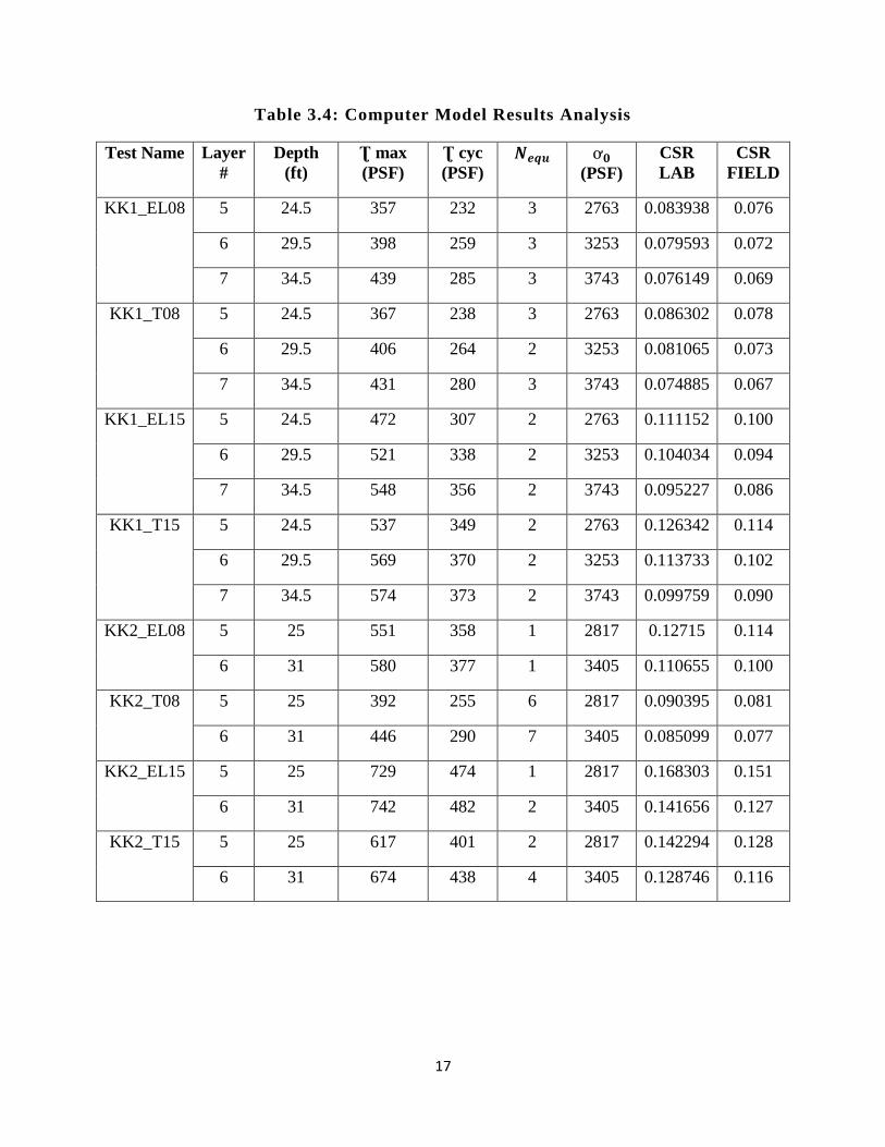
Table 3.4 lists the computer model results at the center of each fly ash layer. The test name is
structured as follows. The first half indicates what profile, KK-1 or KK-2, was tested. The letters
in the second half indicate which earthquake motion was used. “EL” stands for El Centro and
“T” stands for Taft. Lastly, the two-digit number shows which ground acceleration, 0.08g or 0.15
g, was applied in each test. The overburden stress ( was calculated based upon the density and
thickness of each layer above the point of interest. The maximum shear stress for each fly ash

12
layer was taken from the table of maximum shear stress produced for each test. These tables may
be found in Appendix B.
The cyclic stress method of liquefaction potential evaluation is one of the most common methods
used. Because the stress-time history for each layer is irregular, the data had to be normalized in
order to analyze the equivalent number of uniform cycles, . If a cycle exceeded 65% of the
maximum shear stress amplitude, , that cycle counted for one equivalent uniform cycle.
Seed et al. (1975-1) developed this relationship which is expressed in equation 3.2.
(3.2)
65% is the most common value used for this purpose (Kramer, 1996). The cyclic shear stress
amplitude ( was then applied to equation 2.1 to determine the laboratory cyclic stress ratio
( . Seed et al. (1975-2) suggested a correction to the laboratory results to yield a
predication for the field results. Equation 3.3 below was used to correct the laboratory data.
(3.3)
The final field shear stress ratio and the equivalent number of cycles was plotted on the same
chart as the laboratory results. This chart is contained in Figure 3.4. The numbers of equivalent
cycles under field cyclic stress ratios were lower than the cyclic liquefaction tests. This implies
that the critical layers of fly ash will not liquefy.
13
Table 3.2: Site Characteristics of Profile KK-1
Layer Number
Material Description
Thickness (ft)
Unit Weight
(pcf)
Gmax (ksf)
Vs (ft/sec)
Modulus Reduction
Curve
Damping Curve
1 Gravelly Silty Sand 2 108 3213 978 Sand (Seed and Idriss) - Average
Sand (Seed and Idriss) -
Average
2 Sand and Gravel 13 114 3391 978 Sand (Seed and Idriss) - Upper
Sand (Seed and Idriss) -
Upper
3 Sand and Gravel 5 114 3391 978 Sand (Seed and Idriss) - Upper
Sand (Seed and Idriss) -
Upper
4 Silty Clay 2 125 3718 978 Clay (Seed and
Sun 1989)
Clay -Average
(Sun et al. )
5 Fly Ash 5 98 690 478 Sand (Seed and
Idriss 1970) Sand (Idriss
1990)
6 Fly Ash 5 98 690 478 Sand (Seed and
Idriss 1970) Sand (Idriss
1990)
7 Fly Ash 5 98 690 478 Sand (Seed and
Idriss 1970) Sand (Idriss
1990)
8 Fly Ash 5 98 690 478 Sand (Seed and
Idriss 1970) Sand (Idriss
1990)
9 Fly Ash 5 98 690 478 Sand (Seed and
Idriss 1970) Sand (Idriss
1990)
10 Fly Ash 5 98 690 478 Sand (Seed and
Idriss 1970) Sand (Idriss
1990)
11 Fly Ash 5 98 690 478 Sand (Seed and
Idriss 1970) Sand (Idriss
1990)
12 Clay Foundation 10 130 1944 694 Clay (Seed and
Sun 1989)
Clay -Average
(Sun et al. )
13 Silty Clay
Foundaton 20 125 1870 694
Clay (Seed and Sun 1989)
Clay -Average
(Sun et al. )
14 Foundation Soil 20 130 1944 694 Clay (Seed and
Sun 1989)
Clay -Average
(Sun et al. )
15 Sandstone Bedrock Infinite 140 135360 5577 Rock (Idriss) Rock (Idriss)

14
Table 3.3 Site Characteristics of Profile KK-2
Layer Number
Material Description
Thickness (ft)
Unit Weight
(pcf) Gmax (ksf)
Vs (ft/sec)
Modulus Reduction Curve
Damping Curve
1 Silty Clay 1 125 3718 978 Clay (Seed and
Sun 1989) Clay (Idriss
1990)
2 Bottom Ash 2 100 2975 978 Sand (Seed and
Idriss 1970) Sand (Idriss
1990)
3 Gravelly Silty Sand 13 110 3391 996 Sand (Seed and Idriss) - Average
Sand (Seed and Idriss) -
Average
4 Silty Clay 6 128 1915 694 Clay (Seed and
Sun 1989)
Clay -Average
(Sun et al. )
5 Fly Ash 6 98 690 478 Sand (Seed and
Idriss 1970) Sand (Idriss
1990)
6 Fly Ash 6 98 690 478 Sand (Seed and
Idriss 1970) Sand (Idriss
1990)
7 Bottom Ash 8 100 2975 978 Sand (Seed and
Idriss 1970) Sand (Idriss
1990)
8 Silty Clay
Foundation 20 125 1870 694
Clay (Seed and Sun 1989)
Clay -Average
(Sun et al. )
9 Foundation Soil 20 130 1944 694 Clay (Seed and
Sun 1989)
Clay -Average
(Sun et al. )
10 Sandstone Bedrock Infinite 140 135360 5577 Rock (Idriss) Rock (Idriss)

15
Figure 3.2: Soil Profile KK-1
16
Figure 3.3: Soil Profile KK-2
17
Table 3.4: Computer Model Results Analysis
Test Name Layer
#
Depth
(ft)
Ʈ max
(PSF)
Ʈ cyc
(PSF)
(PSF)
CSR
LAB
CSR
FIELD
KK1_EL08 5 24.5 357 232 3 2763 0.083938 0.076
6 29.5 398 259 3 3253 0.079593 0.072
7 34.5 439 285 3 3743 0.076149 0.069
KK1_T08 5 24.5 367 238 3 2763 0.086302 0.078
6 29.5 406 264 2 3253 0.081065 0.073
7 34.5 431 280 3 3743 0.074885 0.067
KK1_EL15 5 24.5 472 307 2 2763 0.111152 0.100
6 29.5 521 338 2 3253 0.104034 0.094
7 34.5 548 356 2 3743 0.095227 0.086
KK1_T15 5 24.5 537 349 2 2763 0.126342 0.114
6 29.5 569 370 2 3253 0.113733 0.102
7 34.5 574 373 2 3743 0.099759 0.090
KK2_EL08 5 25 551 358 1 2817 0.12715 0.114
6 31 580 377 1 3405 0.110655 0.100
KK2_T08 5 25 392 255 6 2817 0.090395 0.081
6 31 446 290 7 3405 0.085099 0.077
KK2_EL15 5 25 729 474 1 2817 0.168303 0.151
6 31 742 482 2 3405 0.141656 0.127
KK2_T15 5 25 617 401 2 2817 0.142294 0.128
6 31 674 438 4 3405 0.128746 0.116

18
Figure 3.4: Combined Results of Laboratory Tests and Computer Models
0
0.05
0.1
0.15
0.2
0.25
0.3
0.35
0.4
0.45
1 10 100 1000
Cyc
lic S
tre
ss R
atio
(C
SR)
Cycles to Liquefaction
Confining stress = 20 psi
Confining Pressure = 40 psi
Profile KK-1, 0.08g
Profile KK-1, 0.15g
Profile KK-2, 0.08g
Profile KK-2, 0.15g
Did not liquefy at 500

19
Chapter 4 Summary and Conclusion
4.1 Summary
Liquefaction can cause extreme structural damage to infrastructure. Since the 1970’s, extensive
research has been done into the liquefaction potential of natural soils. This study examines the
liquefaction potential of Class F fly ash in a storage pond through laboratory experiments and
computer model analysis. Cyclic tests were performed with reconstituted specimens from an
AEP fly ash pond. The results of these tests were used to establish upper and lower bounds of a
liquefaction zone. Computer models of two pond profiles based upon a study provided by AEP
were created. Each profile was analyzed four times using different combinations of ground
acceleration amplitude and earthquake motion. The results from the top layers of fly ash were
plotted on the cyclic laboratory test results to determine if liquefaction would occur and damage
the dike of the pond.
4.2 Conclusions
The following conclusions can be made based on the laboratory testing and numerical analysis
results.
1. The cyclic loading imposed by the input earthquake motion was found to be lower than the
cyclic strength of the Class F fly ash material found in laboratory tests.
2. As the cyclic stress ratio increase, the number of stress cycles to liquefaction decreases.

20
3. The 2005 OSU Class F fly ash study suggested that there was a relationship between the
confining stress and liquefaction potential unlike previous studies of sand. The results of the
current study suggest that liquefaction potential is not significantly dependent on the confining
pressure based upon the range of confining pressures used.
Further study should be done on Class F fly ash from other sources to determine if the suggested
relationship between cycles to liquefaction and confining stress exists in the 2005 OSU study is
valid. Also, further studies with Class F fly ash from other sources will determine if there is
variation in liquefaction potential within this fly ash class.

21
List of References
1. ASTM Designation: ASTM D5311, “Standard Test Method for Load Controlled Cyclic
Triaxial Strength of Soil”, Annual Book of ASTM Standards, 2004, pp. 1167-1176.
2. Kramer, S.L. (1996). Geotechnical Earthquake Engineering, Prentice Hall, Inc., Upper Saddle
River, New Jersey, 653 pp.
3. Seed, H. B. and I. M. Idriss “Soil Moduli and Damping Factors for Dynamic Response
Analysis”. Report No. UCB/EERC-70/10, Earthquake Engineering Research Center, University
of California, Berkeley, 1970.
4. Seed, H.B., K. Mori and C.K. Chan, “Influence of Seismic History on the Liquefaction
Characteristics of Sands”, Report No. UCB/EERC-75/25, Earthquake Engineering Research
Center, University of California, Berkeley, 1975-1.
5. Seed, H.B., K.L. Lee, I.M. Idriss and F.I. Makdisi, “The Slides in the San Fernando Dams
During the Earthquake of February 9, 1971 ”, Journal of Geotechnical Engineering Division,
ASCE, Vol. 101, No. GT7, pp. 651-688, 1975-2.
6. Haldar, A., and W.H. Tang, “Statistical Study of Uniform Cycles in Earthquake Motion”,
Journal of the Geotechnical Engineering Division, ASCE, Vol. 107, No. GT5, pp. 577-589,
1981.
7. Zand, Behrad, et al. "An Experimental Investigation on Liquefaction Potential and Post-
Liquefaction Shear Strength of Impounded Fly Ash." Fuel. 88.7 (2009): 1160-1166. Web. 28
Jan. 2013. <http://www.sciencedirect.com/science/article/pii/S0016236108004018>.

22
8. . "2011 Fly Ash Production and Use Statistics." AACA: Advancing the Management and Use
of Coal Combustion Products. AACA: Advancing the Management and Use of Coal Combustion
Products, 25 Jan 2013. Web. 4 Feb 2013.
<http://acaa.affiniscape.com/associations/8003/files/1966-
2011_FlyAsh_Prod_and_Use_Charts.pdf>.
9. . "ProShake: Ground Response Analysis Program, User's Manual." EduPro Civil Systems,
Inc.. EduPro Civil Systems, Inc., 2 Apr 2012. Web. 4 Feb 2013. <http://www.proshake.com/>.

23
Appendix A: Laboratory Test Results

24
Figure A.1a: Specimen 2R Cyclic Loading
Figure A.1b: Specimen 2R Pore Water Pressure Build-up and Cyclic Displacement
-30
-20
-10
0
10
20
30
0 20 40 60 80 100 120 140
Ax
ial
Str
ess
(p
si)
Cycles
Load Cell
Liquefaction
-0.040
0.000
0.040
0.080
0.120
0.160
0.200
-0.200
0.000
0.200
0.400
0.600
0.800
1.000
1.200
0 10 20 30 40 50 60 70 80 90 100 110 120 130 140 150
Str
ain
(in
/in
)
Ra
tio
of
Ex
ce
ss
Po
re P
ress
ure
to
In
itia
l C
on
fin
ing
Str
ess
(p
si/p
si)
Cycles
Excess Pore Pressure to Confining Stress
Strain (in/in)
Liquefaction

25
Figure A.2a: Specimen 3Cyclic Loading
Figure A.2b: Specimen 3Pore Water Pressure Build-up and Cyclic Displacement
-30
-20
-10
0
10
20
30
0 1 2 3 4 5 6 7 8
Ax
ial
Str
ess
(p
si)
Cycles
Load Cell
Liquefaction
-0.040
0.000
0.040
0.080
0.120
0.160
0.200
-0.200
0.000
0.200
0.400
0.600
0.800
1.000
1.200
0 1 2 3 4 5 6 7 8
Str
ain
(in
/in
)
Ra
tio
of
Ex
ce
ss
Po
re P
ress
ure
to
In
itia
l C
on
fin
ing
Str
ess
(p
si/p
si)
Cycles
Excess Pore Pressure to Confining Stress
Strain (in/in)
Liquefaction

26
Figure A.3a: Specimen 6 Cyclic Loading (Load Cell Response)
Figure A.3b: Specimen 6 Pore Water Pressure Build-up and Cyclic Displacement
-30
-20
-10
0
10
20
30
0 50 100 150 200 250 300 350 400 450 500
Axia
l S
tress (
psi)
Cycles
Load Cell
-0.040
0.000
0.040
0.080
0.120
0.160
0.200
-0.050
0.000
0.050
0.100
0.150
0.200
0.250
0.300
0.350
0.400
0.450
0 50 100 150 200 250 300 350 400 450 500
Str
ain
(in
/in
)
Ra
tio
of
Ex
ce
ss
Po
re P
ress
ure
to
In
itia
l C
on
fin
ing
Str
ess
(p
si/p
si)
Cycles
Excess Pore Pressure to Confining Stress
Strain (in/in)

27
Figure A.4a: Specimen 7 Cyclic Loading
Figure A.4b: Specimen 7 Pore Water Pressure Build-up and Cyclic Displacement
-30
-20
-10
0
10
20
30
0 10 20 30 40 50 60 70 80 90
Axia
l S
tress (
psi)
Cycles
Load Cell
Liquefaction
-0.040
0.000
0.040
0.080
0.120
0.160
0.200
-0.200
0.000
0.200
0.400
0.600
0.800
1.000
1.200
0 10 20 30 40 50 60 70 80 90
Str
ain
(in
/in
)
Ra
tio
of
Ex
ce
ss
Po
re P
ress
ure
to
In
itia
l C
on
fin
ing
Str
ess
(p
si/p
si)
Cycles
Excess Pore Pressure to Confining Stress
Strain (in/in)
Liquefaction

28
Figure A.5a: Specimen 8 Cyclic Loading
Figure A.5b: Specimen 8Pore Water Pressure Build-up and Cyclic Displacement
-30
-20
-10
0
10
20
30
0 2 4 6 8 10 12 14
Axia
l S
tress (
psi)
Cycles
Load Cell
Liquefaction
-0.040
0.000
0.040
0.080
0.120
0.160
0.200
0.000
0.100
0.200
0.300
0.400
0.500
0.600
0.700
0.800
0.900
1.000
0 5 10 15
Str
ain
(in
/in
)
Rati
o o
f E
xcess P
ore
Pre
ssu
re t
o In
itia
l C
on
fin
ing
Str
ess (
psi/p
si)
Cycles
Excess Pore Pressure to Confining Stress
Strain (in/in)
Liquefaction

29
Figure A.6a: Specimen 10 Cyclic Loading (Load Cell Response)
Figure A.6b: Specimen 10 Pore Water Pressure Build-up and Cyclic Displacement
-30
-20
-10
0
10
20
30
0 50 100 150 200 250 300 350 400 450 500
Axia
l S
tress (
psi)
Cycles
Load Cell
-0.040
0.000
0.040
0.080
0.120
0.160
0.200
0.000
0.100
0.200
0.300
0.400
0.500
0.600
0.700
0.800
0.900
0 50 100 150 200 250 300 350 400 450 500
Str
ain
(in
/in
)
Rati
o o
f E
xcess P
ore
Pre
ssu
re t
o In
itia
l C
on
fin
ing
Str
ess (
psi/p
si)
Cycles
Excess Pore Pressure to ConfiningStress
Strain (in/in)
30
Figure A.7a: Specimen 11 Cyclic Loading
Figure A.7a: Specimen 11 Pore Water Pressure Build-up and Cyclic Displacement
-30
-20
-10
0
10
20
30
0 1 2 3 4 5 6 7 8 9 10
Axia
l S
tress (
psi)
Cycles
Load Cell
Liquefaction
-0.040
0.000
0.040
0.080
0.120
0.160
0.200
-0.200
0.000
0.200
0.400
0.600
0.800
1.000
0 1 2 3 4 5 6 7 8 9 10
Str
ain
(in
/in
)
Rati
o o
f E
xcess P
ore
Pre
ssu
re t
o In
itia
l C
on
fin
ing
Str
ess (
psi/p
si)
Cycles
Excess Pore Pressure to Confining Stress
Strain (in/in)
Liquefaction

31
Figure A.8a: Specimen 18 Cyclic Loading
Figure A.8b: Specimen 18 Pore Water Pressure Build-up and Cyclic Displacement
-30
-20
-10
0
10
20
30
0 10 20 30 40 50
Axia
l S
tress (
psi)
Cycles
Load Cell
Liquefaction
-0.040
0.000
0.040
0.080
0.120
0.160
0.200
0.000
0.100
0.200
0.300
0.400
0.500
0.600
0.700
0.800
0.900
1.000
10 20 30 40 50
Str
ain
(in
/in
)
Rati
o o
f E
xcess P
ore
Pre
ssu
re t
o In
itia
l C
on
fin
ing
Str
ess (
psi/p
si)
Cycles
Excess Pore Pressure to Confining Stress
Strain (in/in)
Liquefaction

32
Figure A.9a: Specimen 21 Cyclic Loading
Figure A.9b: Specimen 21 Pore Water Pressure Build-up and Cyclic Displacement
-30
-20
-10
0
10
20
30
0 10 20 30 40 50 60
Axia
l S
tress (
psi)
Cycles
Load Cell
Liquefaction
-0.040
0.000
0.040
0.080
0.120
0.160
0.200
-0.2
0.0
0.2
0.4
0.6
0.8
1.0
0 10 20 30 40 50 60
Str
ain
(in
/in
)
Ra
tio
of
Ex
ce
ss
Po
re P
ress
ure
to
In
itia
l C
on
fin
ing
Str
ess
(p
si/p
si)
Cycles
Excess Pore Pressure to Confining Stress
Strain (in/in)
Liquefaction

33
Figure A.10a: Specimen 81 Cyclic Loading
Figure A.10b: Specimen 81 Pore Water Pressure Build-up and Cyclic Displacement
-30
-20
-10
0
10
20
30
0 20 40 60 80 100 120
Axia
l S
tress (
psi)
Cycles
Load Cell
Liquefaction
-0.200
-0.160
-0.120
-0.080
-0.040
0.000
0.040
0.080
0.120
0.160
0.200
-0.2
0.0
0.2
0.4
0.6
0.8
1.0
0 10 20 30 40 50 60 70 80 90 100 110 120 130
Str
ain
(in
/in
)
Ra
tio
of
Ex
ce
ss
Po
re P
ress
ure
to
In
itia
l C
on
fin
ing
Str
ess
(p
si/p
si)
Cycles
Excess Pore Pressure to Confining Stress
Strain (in/in)
Liquefaction

34
Figure A.11a: Specimen 84 Cyclic Loading
Figure A.11b: Specimen 84 Pore Water Pressure Build-up and Cyclic Displacement
-30
-20
-10
0
10
20
30
0 2 4 6 8 10 12 14 16
Axia
l S
tress (
psi)
Cycles
Load Cell
Liquefaction
-0.100
-0.060
-0.020
0.020
0.060
0.100
0.140
0.180
-0.4
-0.2
0.0
0.2
0.4
0.6
0.8
1.0
1.2
0 2 4 6 8 10 12 14 16
Str
ain
(in
/in
)
Ra
tio
of
Ex
ce
ss
Po
re P
ress
ure
to
In
itia
l C
on
fin
ing
Str
ess
(p
si/p
si)
Cycles
Excess Pore Pressure to Confining Stress
Strain (in/in)
Liquefaction

35
Figure A.12a Specimen 85 Cyclic Loading
Figure A.12b Specimen 85 Pore Water Pressure Build-up and Cyclic Displacement
-30
-20
-10
0
10
20
30
0 2 4 6 8 10 12 14
Ax
ial
Str
ess
(p
si)
Cycles
Load Cell
Liquefaction
-0.080
-0.040
0.000
0.040
0.080
0.120
0.160
0.200
-0.4
-0.2
0.0
0.2
0.4
0.6
0.8
1.0
1.2
0 2 4 6 8 10 12 14
Str
ain
(in
/in
)
Rati
o o
f E
xcess P
ore
Pre
ssu
re t
o In
itia
l C
on
fin
ing
Str
ess (
psi/p
si)
Cycles
Excess Pore Pressure to Confining Stress
Strain (in/in)
Liquefaction

36
Figure A.13a Specimen 86 Cyclic Loading
Figure A.13b Specimen 86 Pore Water Pressure Build-up and Cyclic Displacement
-30
-20
-10
0
10
20
30
0 10 20 30 40 50
Ax
ial
Str
ess
(p
si)
Cycles
Load Cell
Liquefaction
-0.040
0.000
0.040
0.080
0.120
0.160
0.200
-0.2
0.0
0.2
0.4
0.6
0.8
1.0
1.2
0 10 20 30 40 50
Str
ain
(in
/in
)
Rati
o o
f E
xcess P
ore
Pre
ssu
re t
o In
itia
l C
on
fin
ing
Str
ess (
psi/p
si)
Cycles
Excess Pore Pressure to Confining Stress
Strain (in/in)
Liquefaction

37
Figure A.14a Specimen 87 Cyclic Loading
Figure A.14b Specimen 87 Pore Water Pressure Build-up and Cyclic Displacement
-30
-20
-10
0
10
20
30
0 10 20 30 40 50 60 70 80 90 100
Ax
ial
Str
ess
(p
si)
Cycles
Load Cell
Liquefaction
-0.040
0.000
0.040
0.080
0.120
0.160
0.200
-0.2
0.0
0.2
0.4
0.6
0.8
1.0
0 10 20 30 40 50 60 70 80 90 100
Str
ain
(in
/in
)
Ra
tio
of
Ex
ce
ss
Po
re P
ress
ure
to
In
itia
l C
on
fin
ing
Str
ess
(p
si/p
si)
Cycles
Excess Pore Pressure to Confining Stress
Strain (in/in)
Liquefaction
38
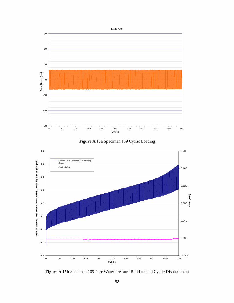
Figure A.15a Specimen 109 Cyclic Loading
Figure A.15b Specimen 109 Pore Water Pressure Build-up and Cyclic Displacement
-30
-20
-10
0
10
20
30
0 50 100 150 200 250 300 350 400 450 500
Ax
ial
Str
ess (
psi)
Cycles
Load Cell
-0.040
0.000
0.040
0.080
0.120
0.160
0.200
0.0
0.1
0.1
0.2
0.2
0.3
0.3
0.4
0.4
0 50 100 150 200 250 300 350 400 450 500
Str
ain
(in
/in
)
Rati
o o
f E
xcess P
ore
Pre
ssu
re t
o I
nit
ial
Co
nfi
nin
g S
tress (
ps
i/p
si)
Cycles
Excess Pore Pressure to ConfiningStress
Strain (in/in)
39
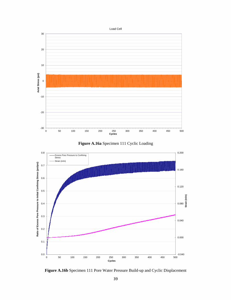
Figure A.16a Specimen 111 Cyclic Loading
Figure A.16b Specimen 111 Pore Water Pressure Build-up and Cyclic Displacement
-30
-20
-10
0
10
20
30
0 50 100 150 200 250 300 350 400 450 500
Ax
ial
Str
ess
(p
si)
Cycles
Load Cell
-0.040
0.000
0.040
0.080
0.120
0.160
0.200
0.0
0.1
0.2
0.3
0.4
0.5
0.6
0.7
0.8
0 50 100 150 200 250 300 350 400 450 500
Str
ain
(in
/in
)
Rati
o o
f E
xcess P
ore
Pre
ssu
re t
o I
nit
ial
Co
nfi
nin
g S
tress (
ps
i/p
si)
Cycles
Excess Pore Pressure to ConfiningStress
Strain (in/in)

40
Figure A.17a Specimen 114 Cyclic Loading
Figure A.17b Specimen 114 Pore Water Pressure Build-up and Cyclic Displacement
-30
-20
-10
0
10
20
30
0 10 20 30 40 50 60 70 80 90 100
Ax
ial
Str
ess
(p
si)
Cycles
Load Cell
Liquefaction
-0.060
-0.020
0.020
0.060
0.100
0.140
0.180
-0.2
0.0
0.2
0.4
0.6
0.8
1.0
0 10 20 30 40 50 60 70 80 90 100
Str
ain
(in
/in
)
Ra
tio
of
Ex
ce
ss
Po
re P
ress
ure
to
In
itia
l C
on
fin
ing
Str
ess
(p
si/p
si)
Cycles
Excess Pore Pressure to Confining Stress
Strain (in/in)
Liquefaction

41
Figure A.18a Specimen 116 Cyclic Loading
Figure A.18b Specimen 116 Pore Water Pressure Build-up and Cyclic Displacement
-30
-20
-10
0
10
20
30
0 15 30 45 60 75 90 105 120 135 150 165 180 195
Axia
l S
tress (
psi)
Cycles
Load Cell
Liquefaction
-0.040
0.000
0.040
0.080
0.120
0.160
0.200
-0.2
0.0
0.2
0.4
0.6
0.8
1.0
1.2
0 15 30 45 60 75 90 105 120 135 150 165 180 195
Str
ain
(in
/in
)
Rati
o o
f E
xcess P
ore
Pre
ssu
re t
o In
itia
l C
on
fin
ing
Str
ess (
psi/p
si)
Cycles
Excess Pore Pressure to Confining Stress
Strain (in/in)
Liquefaction

42
Figure A.19a Specimen 117 Cyclic Loading
Figure A.19b Specimen 117 Pore Water Pressure Build-up and Cyclic Displacement
-30
-20
-10
0
10
20
30
0 50 100 150 200 250 300 350 400 450 500
Axia
l S
tre
ss
(p
si)
Cycles
Load Cell
-0.040
0.000
0.040
0.080
0.120
0.160
0.200
0.0
0.1
0.2
0.3
0.4
0.5
0.6
0.7
0 50 100 150 200 250 300 350 400 450 500
Str
ain
(in
/in
)
Rati
o o
f E
xcess P
ore
Pre
ssu
re t
o I
nit
ial
Co
nfi
nin
g S
tress (
ps
i/p
si)
Cycles
Excess Pore Pressure to ConfiningStress
Strain (in/in)

43
Figure A.20a Specimen 119 Cyclic Loading
Figure A.20b Specimen 119 Pore Water Pressure Build-up and Cyclic Displacement
-30
-20
-10
0
10
20
30
0 5 10 15 20 25 30
Ax
ial
Str
ess
(p
si)
Cycles
Load Cell
Liquefaction
-0.040
0.000
0.040
0.080
0.120
0.160
0.200
-0.2
0.0
0.2
0.4
0.6
0.8
1.0
0 5 10 15 20 25 30
Str
ain
(in
/in
)
Ra
tio
of
Ex
ce
ss
Po
re P
ress
ure
to
In
itia
l C
on
fin
ing
Str
ess
(p
si/p
si)
Cycles
Excess Pore Pressure to Confining Stress
Strain (in/in)
Liquefaction
44
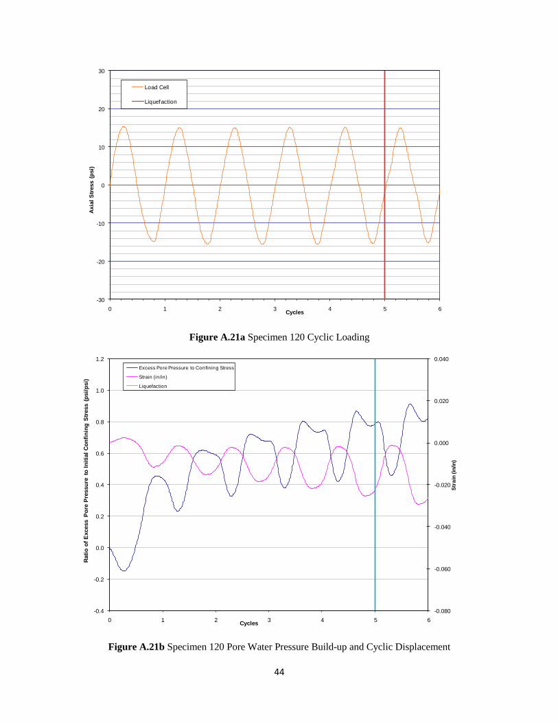
Figure A.21a Specimen 120 Cyclic Loading
Figure A.21b Specimen 120 Pore Water Pressure Build-up and Cyclic Displacement
-30
-20
-10
0
10
20
30
0 1 2 3 4 5 6
Axia
l S
tress (
psi)
Cycles
Load Cell
Liquefaction
-0.080
-0.060
-0.040
-0.020
0.000
0.020
0.040
-0.4
-0.2
0.0
0.2
0.4
0.6
0.8
1.0
1.2
0 1 2 3 4 5 6
Str
ain
(in
/in
)
Rati
o o
f E
xcess P
ore
Pre
ssu
re t
o I
nit
ial
Co
nfi
nin
g S
tress (
psi/
psi)
Cycles
Excess Pore Pressure to Confining Stress
Strain (in/in)
Liquefaction

45
Figure A.22a Specimen 122 Cyclic Loading
Figure A.22b Specimen 122 Pore Water Pressure Build-up and Cyclic Displacement
-30
-20
-10
0
10
20
30
0 5 10 15
Axia
l S
tress (
psi)
Cycles
Load Cell
Liquefaction
-0.100
-0.060
-0.020
0.020
0.060
0.100
0.140
0.180
-0.4
-0.2
0.0
0.2
0.4
0.6
0.8
1.0
1.2
0 5 10 15
Str
ain
(in
/in
)
Ra
tio
of
Ex
ce
ss
Po
re P
ress
ure
to
In
itia
l C
on
fin
ing
Str
ess
(p
si/p
si)
Cycles
Excess Pore Pressure to Confining Stress
Strain (in/in)
Liquefaction
46
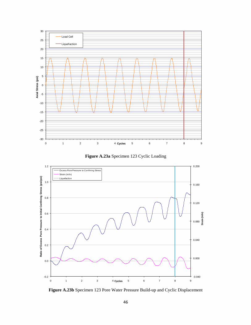
Figure A.23a Specimen 123 Cyclic Loading
Figure A.23b Specimen 123 Pore Water Pressure Build-up and Cyclic Displacement
-30
-25
-20
-15
-10
-5
0
5
10
15
20
25
30
0 1 2 3 4 5 6 7 8 9
Axia
l S
tress (
psi)
Cycles
Load Cell
Liquefaction
-0.040
0.000
0.040
0.080
0.120
0.160
0.200
-0.2
0.0
0.2
0.4
0.6
0.8
1.0
1.2
0 1 2 3 4 5 6 7 8 9
Str
ain
(in
/in
)
Rati
o o
f E
xcess P
ore
Pre
ssu
re t
o I
nit
ial
Co
nfi
nin
g S
tress (
psi/
psi)
Cycles
Excess Pore Pressure to Confining Stress
Strain (in/in)
Liquefaction
47
Appendix B: Ground Response Analysis Results

48
Input B.1: KK-1 Soil Profile Input Results

49

50
Input B.2: KK-2 Soil Profile Input Results

51

52
Analysis B.1: KK-1 Profile with El Centro Earthquake Motion at 0.08g Ground Acceleration

53

54

55
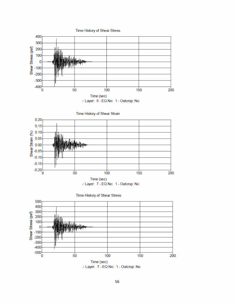
Analysis B.2: KK-1 Profile with Taft Earthquake Motion at 0.08g Ground Acceleration
56

57

58
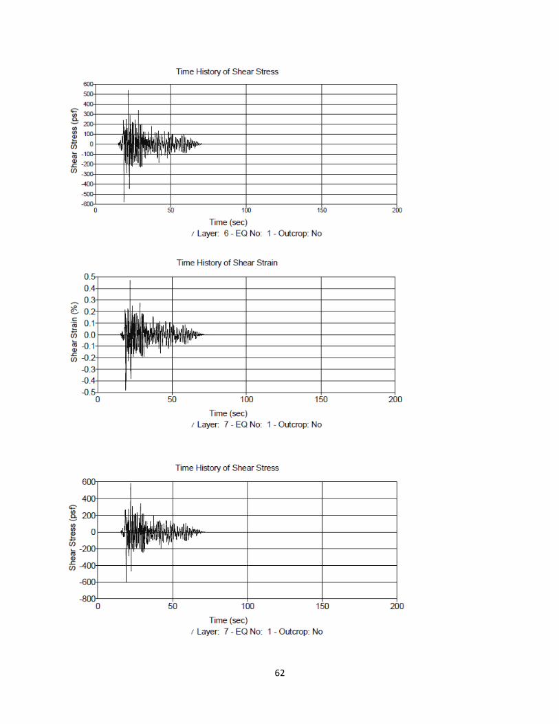
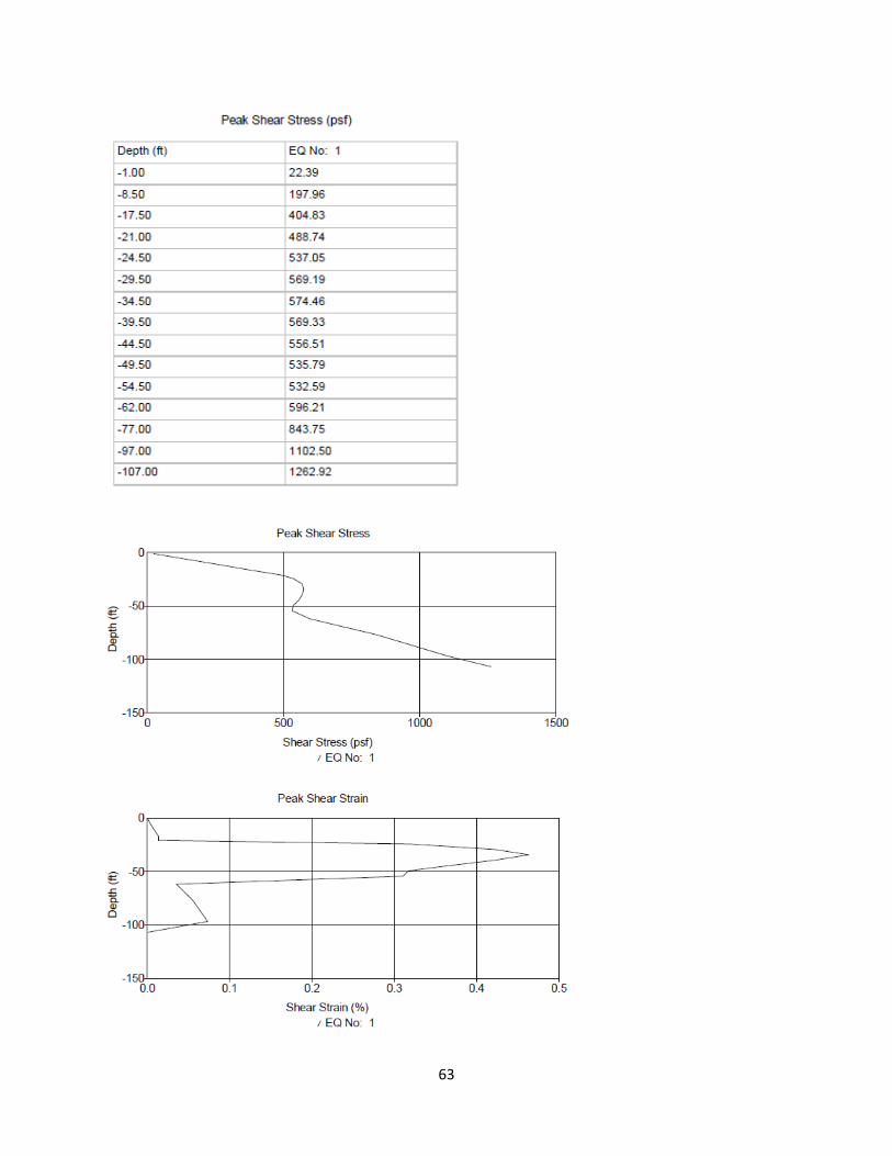
Analysis B.3: KK-1 Profile with El Centro Earthquake Motion at 0.15g Ground Acceleration

59

60
Peak Shear Stress

61
Analysis B.4: KK-1 Profile with Taft Motion at 0.15g Ground Acceleration
62
63

64
Analysis B.5: KK-2 Profile with El Centro Earthquake Motion at 0.08g Ground Acceleration

65

66

67
Analysis B.6: KK-2 Profile with Taft Earthquake Motion at 0.08g Ground Acceleration

68

69

70
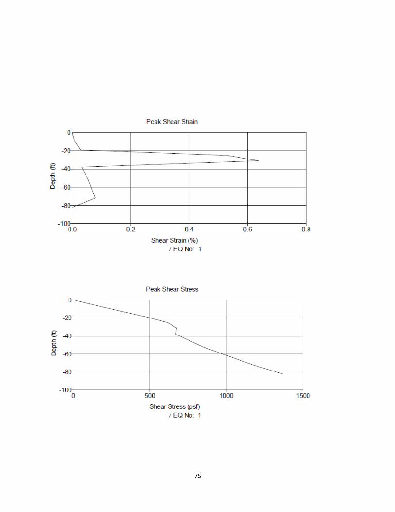
Analysis B.7: KK-2 Profile with El Centro Earthquake Motion at 0.15g Ground Acceleration
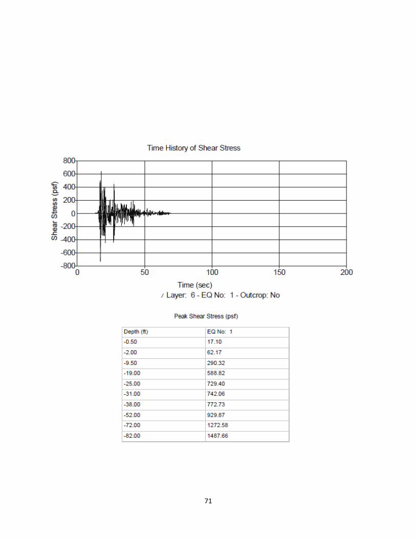
71

72

73
Analysis B.8: KK-2 Profile with Taft Earthquake Motion at 0.15g Ground Acceleration

74
75