evaluation of methods for improving classifying … · be more practical than screens for fine...
TRANSCRIPT

EVALUATION OF METHODS FOR IMPROVING CLASSIFYING CYCLONE PERFORMANCE
by
Dongcheol Shin
Thesis submitted to the Faculty of the Virginia Polytechnic Institute and State University
in partial fulfillment of the requirements for the degree of
MASTER OF SCIENCE
in
Mining and Minerals Engineering
Graduate Committee Members
Gerald H. Luttrell Roe-Hoan Yoon Gregory T. Adel
May 10, 2007 Blacksburg, Virginia
Keywords: Hydrocyclone, Classification, Linear Circuit Analysis
Copyright 2007, Dongcheol Shin

EVALUATION OF METHODS FOR IMPROVING CLASSIFYING CYCLONE PERFORMANCE
by
Dongcheol Shin
Committee Chairman: Gerald H. Luttrell Department of Mining and Minerals Engineering
ABSTRACT
Most mineral and coal processing plants are forced to size their particulate streams in
order to maximize the efficiency of their unit operations. Classifiers are generally considered to
be more practical than screens for fine sizing, but the separation efficiency decreases
dramatically for particles smaller than approximately 150 µm. In addition, classifiers commonly
suffer from bypass, which occurs when a portion of the ultrafine particles (slimes) are misplaced
by hydraulic carryover into the oversize product. The unwanted misplacement can have a large
adverse impact on downstream separation processes. One method of reducing bypass is to inject
water into the cyclone apex. Unfortunately, existing water injection systems tend to substantially
increase the particle cut size, which makes it unacceptable for ultrafine sizing applications. A
new apex washing technology was developed to reduce the bypass of ultrafine material to the
hydrocyclone underflow while maintaining particle size cuts in the 25-50 µm size range.
Another method of reducing bypass is to retreat the cyclone underflow using multiple
stages of classifiers. However, natural variations in the physical properties of the feed make it
difficult to calculate the exact improvement offered by multistage classification in experimental
studies. Therefore, several mathematical equations for multistage classification circuits were
evaluated using mathematical tools to calculate the expected impact of multistage hydrocyclone
circuits on overall cut size, separation efficiency and bypass. These studies suggest that a two-
stage circuit which retreats primary underflow and recycles secondary overflow offers the best
balance between reducing bypass and maintaining a small cut size and high efficiency.

iii
ACKNOWLEDGMENTS
The author would like to express the deepest appreciation to his advisor, Dr. Gerald H.
Luttrell, for his guidance and advice during this investigation. His invaluable knowledge and
experience in mineral processing gave the author a lot of motivation to complete this research.
Deepest appreciation also goes to Dr. Roe-Hoan Yoon for his suggestions and recommendations.
The author is also grateful to Dr. Greg Adel for his class teaching in the area of population
balance modeling. The author is also thanks to Dr. Tom Novak for his guidance in graduate
school life.
A sincere thank you is also expressed to Dr. Jinming Zhang for his friendship and
guidance. Special thanks are also expressed to James Waddell and Robert Bratton for their
technical suggestions and assistance during this investigation. Thanks are extended to Baris
Yazgan, Todd Burchett, Chris Barbee, Kwangmin Kim, Hyunsun Do, Jinhong Zhang, Nini Ma
and Jialin Wang for their friendship.
Thanks are also expressed to several companies whose support made this work possible.
This gratitude is expressed to Toms Creek Coal Company, Coal Clean Company, Middle Fork
Processing, Krebs Engineers and Morris Coker Equipment. Individual thanks must also be
expressed to Mr. Robert Moorhead at Krebs Engineers.
The author would like to thank his parents, Yoonseok Shin and Kyunghee Choi, for their
continued support and encouragement. The author would like to thank his brother, Jinuk Shin,
for his encouragement. The author would like to thank to Myoung-Sin Kim, Dr. Roe-Hoan
Yoon’s wife, for her moral support during the author’s stay in Blacksburg. The author especially
expresses his deepest appreciation to his wife, Jaehee Song, for her support, encouragement and
love. Thanks and loves are expressed to Kate Jiyoung Shin, his adorable daughter, for being with
the author and his wife.

iv
TABLE OF CONTENTS
ABSTRACT.................................................................................................................................... ii
ACKNOWLEDGMENTS ............................................................................................................. iii
TABLE OF CONTENTS............................................................................................................... iv
LIST OF FIGURES ....................................................................................................................... vi
LIST OF TABLES....................................................................................................................... viii
CHAPTER 1 - DEVELOPMENT OF A NEW WATER-INJECTION SYSTEM FOR CLASSIFYING CYCLONES .........................................................................................................1
1.1 Introduction.......................................................................................................................... 1 1.1.1 Background................................................................................................................... 1 1.1.2 Objectives ..................................................................................................................... 1
1.2 Experimental ........................................................................................................................ 3 1.2.1 Description of the Water-Injection System................................................................... 3 1.2.2 Test Circuit Setup ......................................................................................................... 4 1.2.3 Test Procedures............................................................................................................. 7
1.2.3.1 Test Sample............................................................................................................ 7 1.2.3.2 Preliminary Testing................................................................................................ 8 1.2.3.3 Detailed Testing ................................................................................................... 10
1.3 Results and Discussion ...................................................................................................... 14 1.3.1 Parametric Study Results ............................................................................................ 14 1.3.2 Verification Results .................................................................................................... 18 1.3.3 Optimization Results................................................................................................... 19
1.3.3.1 Optimum Conditions for the 20-25 µm Size Range ............................................ 25 1.3.3.2 Optimum Conditions for the 25-30 µm Size Range ............................................ 25 1.3.3.3 Optimum Conditions for the 30-35 µm Size Range ............................................ 26 1.3.3.4 Optimum Conditions for the 35-40 µm Size Range ............................................ 26 1.3.3.5 Optimum Conditions for the 40-45 µm Size Range ............................................ 27 1.3.3.6 Bypass and Cutsize Correlation Under Optimum Conditions ............................. 27
1.4 Summary and Conclusions ................................................................................................ 29
1.5 References.......................................................................................................................... 30
CHAPTER 2 – MATHEMATICAL SOLUTIONS TO PARITIONING EQUATIONS FOR MULTISTAGE CLASSIFICATION CIRCUITS .........................................................................32
2.1 Introduction........................................................................................................................ 32 2.1.1 Background................................................................................................................. 32

v
2.1.2 Linear Circuit Analysis ............................................................................................... 33 2.1.3 Objectives ................................................................................................................... 34
2.2 Mathematical Software ...................................................................................................... 35 2.2.1 Mathematica Simulations............................................................................................ 35 2.2.2 Excel Simulations ....................................................................................................... 38
2.3 Results................................................................................................................................ 40 2.3.1 Underflow Reprocessing Circuit Without Recycle...................................................... 40
2.3.1.1 Two-Stage Circuit Analysis................................................................................. 40 2.3.1.2 Three-Stage Circuit Analysis............................................................................... 44
3.3.2 Underflow Reprocessing Circuit With Recycle.......................................................... 45 2.3.2.1 Two-Stage Circuit Analysis................................................................................. 45 2.3.2.2 Three-Stage Circuit Analysis............................................................................... 46
2.3.3 Overflow Reprocessing Circuit Without Recycle........................................................ 48 2.3.3.1 Two-Stage Circuit Analysis................................................................................. 48 2.3.3.2 Three-Stage Circuit Analysis............................................................................... 49
2.3.4 Overflow Reprocessing Circuit With Recycle............................................................. 50 2.3.4.1 Two-Stage Circuit Analysis................................................................................. 50 2.3.4.2 Three-Stage Circuit Analysis............................................................................... 52
2.4 Generalized Partitioning Expressions................................................................................ 54 2.4.1 Underflow Reprocessing Circuit Without Recycle..................................................... 54 2.4.2 Underflow Reprocessing Circuit With Recycle.......................................................... 55 2.4.3 Overflow Reprocessing Circuit Without Recycle....................................................... 57 2.4.4 Overflow Reprocessing Circuit With Recycle............................................................ 58
2.5 Summary and Conclusions ................................................................................................ 61
2.6 References.......................................................................................................................... 63
APPENDIX I .................................................................................................................................64
Detailed Parametric Test Matrix............................................................................................... 65
Tabular Summary of Parametric Test Results ........................................................................ 167
VITA............................................................................................................................................168

vi
LIST OF FIGURES
Figure 1.1 – Cutaway view and photograph of the water-injected apex. ....................................... 4
Figure 1.2 – Test circuit used to evaluate the water injection apex. ............................................... 5
Figure 1.3 – Control and metering systems used with the water injected apex.............................. 6
Figure 1.4 – Operating principle for the proportional sampler. ...................................................... 7
Figure 1.5 – Flow and pressure response as a function of apex and vortex sizes for the 6-inch (15.2-cm) diameter Krebs G-Max cyclone used in the test program......................... 8
Figure 1.6 – Effect of water injection on hydrocyclone partitioning performance. ..................... 10
Figure 1.7 – Partitioning data from replicate tests conducted under identical test conditions (0 level settings) for the water-injected apex (with 10% error bars)............................ 13
Figure 1.8 – Correlation between actual and predicted cut size and bypass................................. 15
Figure 1.9 – Effect of water injection rate on cutsize and bypass under central point conditions (0.75 inch apex inlet, 4 inch chamber, 1 inch outlet)............................................... 16
Figure 1.10 – Effect of apex outlet diameter on cutsize and bypass under central point conditions (0.75 inch apex inlet, 4 inch chamber, 20 GPM water rate). ................................... 16
Figure 1.11 – Effect of apex inlet diameter (top two plots) and chamber diameter (bottom two plots) on cutsize and bypass..................................................................................... 17
Figure 1.12 – Partitioning performance as a function of water injection rate under central point conditions (0.75 inch apex inlet, 4 inch chamber, 1 inch outlet). ............................ 18
Figure 1.13 – Cutsize response at the optimum point for 20~25 µm classification. .................... 20
Figure 1.14 – Bypass response at the optimum point for 20~25 µm classification...................... 20
Figure 1.15 – Cutsize response at the optimum point for 25~30 µm classification. .................... 21
Figure 1.16 – Bypass response at the optimum point for 25~30 µm classification...................... 21
Figure 1.17 – Cutsize response at the optimum point for 30~35 µm classification. .................... 22
Figure 1.18 – Bypass response at the optimum point for 30~35 µm classification...................... 22
Figure 1.19 – Cutsize response at the optimum point for 35~40 µm classification. .................... 23
Figure 1.20 – Bypass response at the optimum point for 35~40 µm classification...................... 23

vii
Figure 1.21 – Cutsize response at the optimum point for 40~45 µm classification. .................... 24
Figure 1.22 – Bypass response at the optimum point for 40~45 µm classification...................... 24
Figure 1.23 – Correlation between predicted cutsize and bypass. ................................................ 28
Figure 2.1 – Multistage classifier simulation using a spreadsheet-based model (example shows three-stage overflow reprocessing circuit with recycle). ......................................... 38
Figure 2.2 – Schematic of a two-stage underflow reprocessing circuit without recycle. ............. 40
Figure 2.3 – Example of the partitioning response of the two-stage circuit underflow reprocessing circuit without recycle. ....................................................................... 42
Figure 2.4 – Schematic of a three-stage underflow reprocessing circuit without recycle. ........... 44
Figure 2.5 – Schematic of a two-stage underflow reprocessing circuit with recycle. .................. 46
Figure 2.6 – Schematic of a three-stage underflow reprocessing circuit with recycle. ................ 47
Figure 2.7 – Schematic of a two-stage overflow reprocessing circuit without recycle. ............... 48
Figure 2.8 – Schematic of a three-stage overflow reprocessing circuit without recycle. ............. 50
Figure 2.9 – Schematic of a two-stage overflow reprocessing circuit with recycle. .................... 51
Figure 2.10 – Schematic of a three-stage overflow reprocessing circuit with recycle. ................ 52
Figure 2.11 – Generic configurations of underflow reprocessing circuits without recycle.......... 54
Figure 2.12 – Generic configurations of underflow reprocessing circuits with recycle. .............. 56
Figure 2.13 – Generic configurations of overflow reprocessing circuits without recycle............ 57
Figure 2.14 – Generic configurations of overflow reprocessing circuits with recycle. ................ 59

viii
LIST OF TABLES
Table 1.1 – Variables used in the parametric study to evaluate the effects of various operating and geometric variables on apex washing performance. ......................................... 12
Table 1.2 – Regression expressions obtained from the Box-Behnken parametric study.............. 14
Table 1.3 – Optimized conditions for the 20~25 µm cutsize range.............................................. 20
Table 1.4 – Optimized conditions for the 25~30 µm cutsize range.............................................. 21
Table 1.5 – Optimized conditions for the 30~35µm cutsize range............................................... 22
Table 1.6 – Optimized conditions for the 35~40 µm cutsize range.............................................. 23
Table 1.7 – Optimized conditions for the 40~45µm cutsize range............................................... 24
Table 1.8 – Summary of optimal conditions needed for different cutsize ranges. ....................... 25
Table 2.1 – Comparison of Mathematica and Excel determined partition factors for the two-stage underflow reprocessing circuit without recycle....................................................... 43

1
CHAPTER 1 - DEVELOPMENT OF A NEW WATER-INJECTION SYSTEM FOR CLASSIFYING CYCLONES
1.1 Introduction
1.1.1 Background
Most mineral and coal processing plants are forced to size their particulate streams in
order to maximize the efficiency of their unit operations. These sizing techniques commonly
include various types of screens and classifiers. Screens exploit differences in the physical
dimensions of particles by allowing fines to pass through a perforated plate or open mesh while
coarser solids are retained. Unfortunately, screening systems are generally limited to particle size
separations coarser than approximately 250 µm due to limitations associated with capacity and
blinding. Hydraulic classifiers, which include both static and centrifugal devices, are generally
employed for finer size separations. Hydraulic classifiers exploit differences in the settling rates
of particles and are influenced by factors such as particle shape and density as well as particle
size. Classifiers are generally considered to be more practical than screens for fine sizing, but the
separation efficiency decreases dramatically for particles smaller than approximately 150 µm
(Heiskanen, 1993). In addition, classifiers commonly suffer from bypass, which occurs when a
portion of the ultrafine particles (slimes) are misplaced by hydraulic carryover into the oversize
product. The unwanted misplacement can have a large adverse impact on downstream separation
processes.
1.1.2 Objectives
The primary objective of the work outlined in this chapter is to evaluate a new apex
washing system for hydrocyclone classification. The new technology is designed to reduce the

2
bypass of ultrafine material to the hydrocyclone underflow while maintaining particle size
separations in the 25-50 µm size range. The work required the construction and testing of a 6-
inch (15.2-cm) diameter hydrocyclone in a closed-loop test circuit. To optimize the operating
and design parameters associated with the water-injected apex, an optimization study was carried
out using the Box-Behnken method statistical design of experiments. Analysis of the data from
this parametric study was performed using a statistics program known as “Design Expert”. The
optimization was performed in order to determine the conditions that would provide the smallest
amount of bypass while maintaining the size of separation (i.e., cut size) within a fixed narrow
range. In this particular study, the optimum injection water flow rate and combination of
dimensions for the water injection apex were established for five different size ranges (i.e., 20-25,
25-30, 30-35, 35-40 and 40-45 µm).
3
1.2 Experimental
1.2.1 Description of the Water-Injection System
Water-injected apex systems have been shown to be capable of reducing the bypass of
ultrafine particles that are misplaced to the hydrocyclone underflow. Unfortunately, past studies
have shown that existing water injection systems tend to substantially increase the particle
cutsize, which makes these systems unacceptable for many ultrafine sizing applications. In
addition, existing systems typically require large amounts of clarified injection water that may
not be readily available in industrial plants. In light of these problems, a new type of water-
injected cyclone technology was designed by Krebs Engineers to overcome some of the inherent
limitations associated with existing apex washing systems. In particular, the system was designed
to efficiently reduce the bypass of ultrafine particles to the underflow while maintaining a
relatively small particle cutsize.
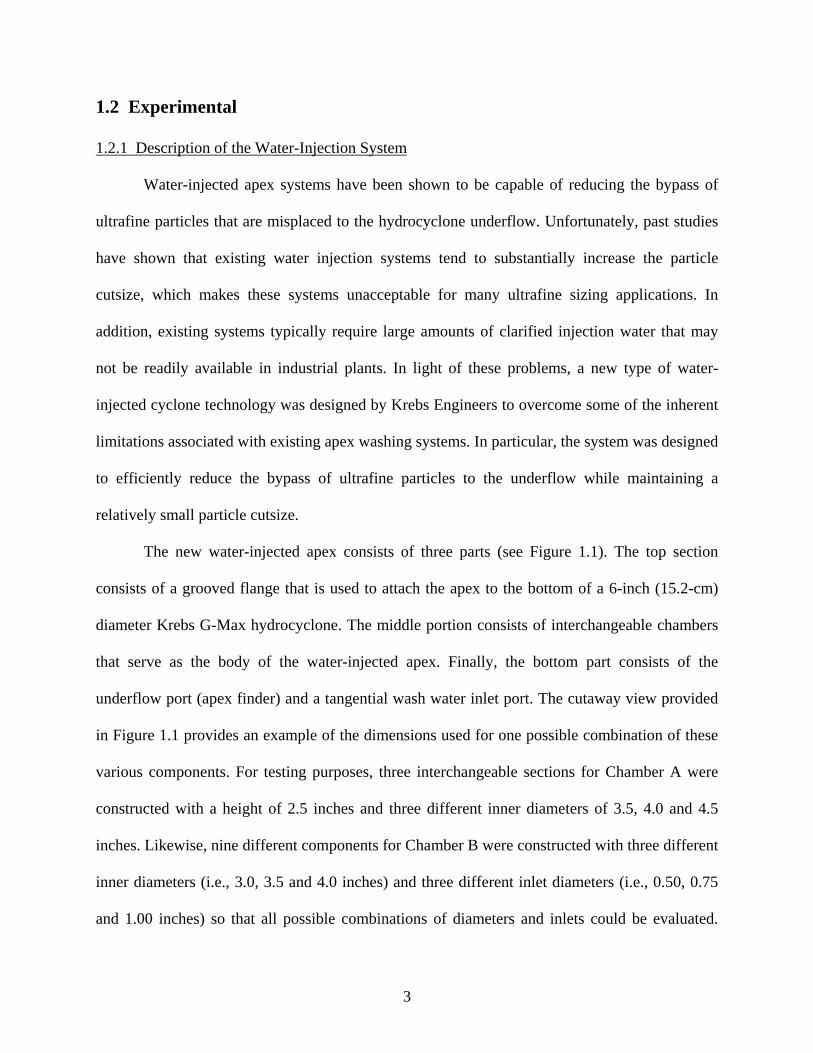
The new water-injected apex consists of three parts (see Figure 1.1). The top section
consists of a grooved flange that is used to attach the apex to the bottom of a 6-inch (15.2-cm)
diameter Krebs G-Max hydrocyclone. The middle portion consists of interchangeable chambers
that serve as the body of the water-injected apex. Finally, the bottom part consists of the
underflow port (apex finder) and a tangential wash water inlet port. The cutaway view provided
in Figure 1.1 provides an example of the dimensions used for one possible combination of these
various components. For testing purposes, three interchangeable sections for Chamber A were
constructed with a height of 2.5 inches and three different inner diameters of 3.5, 4.0 and 4.5
inches. Likewise, nine different components for Chamber B were constructed with three different
inner diameters (i.e., 3.0, 3.5 and 4.0 inches) and three different inlet diameters (i.e., 0.50, 0.75
and 1.00 inches) so that all possible combinations of diameters and inlets could be evaluated.

4
Finally, three interchangeable apexes were constructed with outlet diameters of 0.75, 1.00 and
1.25 inches. The height of the top section, which attached to the bottom of the hydrocyclone, was
kept constant at 16 inches (including the thickness of the supporting plate). The relatively long
height of the cylinder of the topmost section was specifically chosen to increase the retention
time of slurry and water within the apex. Six supporting clips were used to hold the various
sections together and to prevent leaking problems between the joints.
1.2.2 Test Circuit Setup
The experimental test program required the construction of a complete closed-loop test
circuit. A schematic of the test circuit is provided in Figure 1.2. The circuit, which was designed
to be extremely flexible, incorporated a 6-inch (15.2-cm) diameter Krebs G-Max classifying
3.5, 4.0, 4.53.5, 4.0, 4.5
Figure 1.1 – Cutaway view and photograph of the water-injected apex.

5
cyclone with interchangeable components, an electronically controlled variable speed circulation
pump, and an integrated linear-pass proportional sample cutter. The hydrocyclone and slurry
pump equipment were donated by Krebs Engineers and Morris Coker Equipment, respectively,
as a cost-sharing contribution to the project. The pressure and volumetric flow rate of both the
feed slurry and injection water were monitored by an instrument pack. The flow rate and
pressure of the injection water was monitored using a mechanical flow meter and a rotary
pressure gauge, respectively. A photograph showing the valve configuration and metering
system is provided in Figure 1.3. A centrifugal pumping system connected to the town municipal
water supply was used to provide a flow rate of up to 30 GPM of fresh water to the water-
injected apex.
Figure 1.2 – Test circuit used to evaluate the water injection apex.

6
Samples of the overflow and underflow streams from the hydrocyclone were obtained
using a linear-action proportional sampler (see Figure 1.4). The proportional sampler made it
possible to reconstitute the feed stream from the weights of the two product samples. To ensure
the samples were reliable, the reconstituted feed stream was compared with an independent
sample of feed slurry taken from the return pipe that discharged into the sump. To reduce
manpower and reduce operator bias, the motion of the proportional sample cutters was
automated using a pneumatic ram and microprocessor. The automated system made it possible to
accurately input and control both the number of sample cuts (which was input via pushbuttons on
the circuit control panel) and linear velocity of the cutters (which was adjusted by changing the
air pressure on the pneumatic ram).
Figure 1.3 – Control and metering systems used with the water injected apex.

7
1.2.3 Test Procedures
1.2.3.1 Test Sample
During the process of collecting data, bench-scale 6-inch (15.2-cm) hydrocyclone tests
were conducted using flotation feed samples from the Toms Creek coal preparation plant. The
plant is owned and operated by Alpha Natural Resources. The particle size distribution of this
sample was nominally 0.15 mm x 0 (100 mesh x 0). Wet sieving indicated that the sample was a
good candidate for ultrafine particle separation since about 70% of the sample by weight was
finer than 45 µm (325 mesh). The as-received solids content of the sample was found be about
6.5% by weight. Therefore, the solids content was diluted down to the 4.5~5.0% range prior to
Sump/Pump
U/FSample
O/FSample
FeedMake-Up
ProportionalSampler
WaterInjectionCyclone Water
Port
Operation Before Sampling
Sump/Pump
U/FSample
O/FSample
FeedMake-Up
ProportionalSampler
WaterInjectionCyclone Water
Port
Operation During Sampling
Figure 1.4 – Operating principle for the proportional sampler.

8
testing to better match the feed solids content of slurry typically treated by desliming cyclones at
operating plant sites in the coal industry.
1.2.3.2 Preliminary Testing
Several preliminary test runs were conducted to determine the appropriate vortex finder
size for the test program. In these tests, the effects of vortex finder and apex geometries on
pressure drop and volumetric flow rate were evaluated. These initial experiments were carried
out using water and minus 100 mesh coal slurry having a solids content of approximately 4.6%
solids by weight. The pressure drop across the cyclone was measured by taking the difference
between the feed pressure at the cyclone inlet and the overflow pressure at the vortex outlet. The
effects of changes to the hydrocyclone geometry on pressure drop and volumetric flow rate are
summarized in Figure 1.5.
Figure 1.5 – Flow and pressure response as a function of apex and vortex sizes for the 6-inch (15.2-cm) diameter Krebs G-Max cyclone used in the test program.
PRESSURE DROP & USGPM
0
20
40
60
80
100
120
140
160
180
200
1 10 100
PRESSURE DROP (PSI)
VO
LUM
ETR
IC F
LOW
RATE
Apex ø1.25 (VFø2.5, coal slurry)Apex ø1.0 (VFø2.5, coal slurry)Apex ø0.75 (VFø2.5, coal slurry)Apex ø1.25 (VFø2.5, w ater)Apex ø1.0 (VFø2.5, w ater)Apex ø0.75 (VFø2.5, w ater)Apex ø1.25 (VFø1.5, coal slurry)Apex ø1.0 (VFø1.5, coal slurry)Apex ø0.75 (VFø1.5, coal slurry)Apex ø1.25 (VFø1.5, w ater)Apex ø1.0 (VFø1.5, w ater)Apex ø0.75 (VFø1.5, w ater)

9
The data provided in Figure 1.5 show that the size of the vortex finder and pressure drop
is interdependent. In addition, the data demonstrate that the hydrocyclone can pass more slurry at
a given pressure than water. A larger vortex finder results in a lower pressure drop for the same
volume or a greater capacity for the same pressure drop. Conversely, a small diameter vortex
finder result in a larger pressure drop for the same volume. Although particle size analyses were
not conducted on these particular samples, an increase in cyclone pressure drop usually leads to a
higher volumetric throughput and a finer particle cut size (Svarovsky, 1984). Therefore, based on
these results, a 1.5-inch (3.8-cm) diameter vortex finder was selected for the test program since it
could provide a higher pressure drop at given volumetric flow rate for the new water-injected
apex system.
A few preliminary test runs were also performed to compare the performance of the
standard conventional apex and the water-injected apex prior to the initiation of extensive
detailed testing. These initial tests were conducted using a 1.5-inch (3.8-cm) diameter vortex
finer and a constant 120 GPM volumetric slurry flow rate. The experiments were carried out
using water and minus 100 mesh coal slurry having a solids content of approximately 4.5%
solids by weight. The resultant test data shown in Figure 1.6 indicate that the new water-injected
apex has the ability to achieve much better classification performance with a low pressure drop.
In fact, the particle size partition curve obtained at a pressure drop of 26 PSI with a 1-inch
diameter water-washed apex was nearly identical to the curve obtained at a much higher pressure
drop of 32 PSI with a smaller 0.75-inch diameter conventional apex. The ability to operate with a
larger apex has substantial advantages in term of being less prone to plugging. In addition, these
results suggest that the new water-injection apex may make it possible to achieve finer particle
size separations with larger diameter (higher capacity) cyclones in the future.

10
1.2.3.3 Detailed Testing
After completing the preliminary tests, a detailed test program was undertaken to better
identify the operational capabilities of the new water-injection apex. All of the detailed tests
were conducted using the 6-inch (15.2-cm) diameter classifying cyclone equipped with a 1.5-
inch (3.8-cm) diameter vortex finder. Different geometrical combinations of apex inlet, outlet
and diameter were examined for the water-injected system. In each test run, two sets of samples
were collected under steady-state conditions for the same performance. The first sample was
used to determine the total solid contents and head ash contents of the feed, overflow and
underflow streams. The second identical sample was subjected to laboratory particle size
Figure 1.6 – Effect of water injection on hydrocyclone partitioning performance.

11
analysis. Particle size analysis was performed by wet sieving particles larger than 45 µm (325
mesh) and by laser analysis (Microtrac) of particles finer than 45 µm (325 mesh).
The sample point for the feed stream was the discharge of slurry from the return line that
circulated back to the slurry sump. Sample points for the underflow and overflow streams were
cut by the linear proportional cutter located inside the automated sampler. The total volume of
each slurry sample was reduced to a manageable volume by representatively subdividing the
slurry into smaller lots using a wet rotary slurry splitter. Because of the use of a closed-loop
system, the addition of injection water increased the volume of circulating slurry which, in turn,
raised the sump level and reduced the feed solids content. To overcome this problem, a small
dosage of flocculant was added to the circulating feed sump after each series of test runs to
quickly aggregate and settle coal particles. Once settled, some of the clarified water at the top of
the sump was pumped out to restore the solids content of the feed slurry back to the desired
range of 4.5-5.0% by weight. Comparison studies showed that the required flocculant dosage
was too low to impact the sizing performance of the hydrocyclone due to the high levels of shear
within the centrifugal feed pump, piping network and cyclone.
All of the detailed tests were conducted using a volumetric feed slurry flow rate of 100
GPM, which typically provided a pressure drop across the cyclone of 21 PSI. Figure 1.5
indicates that this pressure drop is appropriate for the 6-inch (15.2-cm) diameter hydrocyclone
used in this study. The detailed tests were run in accordance with a Box-Behnken parametric test
matrix developed using the Design Expert™ software package. Four parameters were varied (i.e.,
water injection flow rate, apex outlet diameter, apex inlet diameter and apex chamber diameter)
to create a 30 point test matrix for the water-injected apex system. The lower, middle and upper
settings for each of these parameters are summarized in Table 1.1. As shown, the water injection
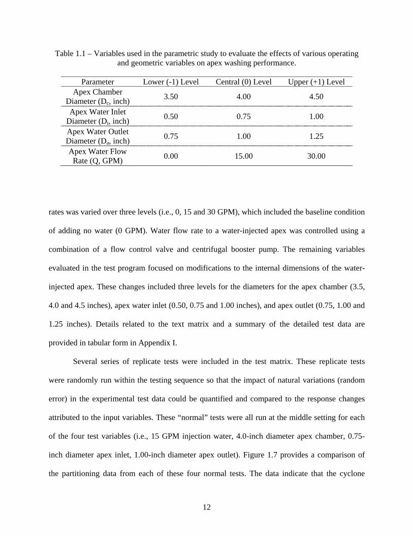
12
rates was varied over three levels (i.e., 0, 15 and 30 GPM), which included the baseline condition
of adding no water (0 GPM). Water flow rate to a water-injected apex was controlled using a
combination of a flow control valve and centrifugal booster pump. The remaining variables
evaluated in the test program focused on modifications to the internal dimensions of the water-
injected apex. These changes included three levels for the diameters for the apex chamber (3.5,
4.0 and 4.5 inches), apex water inlet (0.50, 0.75 and 1.00 inches), and apex outlet (0.75, 1.00 and
1.25 inches). Details related to the text matrix and a summary of the detailed test data are
provided in tabular form in Appendix I.
Several series of replicate tests were included in the test matrix. These replicate tests
were randomly run within the testing sequence so that the impact of natural variations (random
error) in the experimental test data could be quantified and compared to the response changes
attributed to the input variables. These “normal” tests were all run at the middle setting for each
of the four test variables (i.e., 15 GPM injection water, 4.0-inch diameter apex chamber, 0.75-
inch diameter apex inlet, 1.00-inch diameter apex outlet). Figure 1.7 provides a comparison of
the partitioning data from each of these four normal tests. The data indicate that the cyclone
Table 1.1 – Variables used in the parametric study to evaluate the effects of various operating and geometric variables on apex washing performance.
Parameter Lower (-1) Level Central (0) Level Upper (+1) Level
Apex Chamber Diameter (Dc, inch) 3.50 4.00 4.50
Apex Water Inlet Diameter (Di, inch) 0.50 0.75 1.00
Apex Water Outlet Diameter (Da, inch) 0.75 1.00 1.25
Apex Water Flow Rate (Q, GPM) 0.00 15.00 30.00

13
performance was very stable with an overall error of less than 10% error in the partitioning
curves. The particle cutsize determined from the partition curves varied from just 26 to 29 µm,
while the ultrafine bypass varied between 20 to 25% for all replicate tests.
Figure 1.7 – Partitioning data from replicate tests conducted under identical test conditions (0 level settings) for the water-injected apex (with 10% error bars).

14
1.3 Results and Discussion
1.3.1 Parametric Study Results
To fully investigate the effects of the operating and geometric parameters on sizing
performance, regression equations for cutsize and bypass were obtained from the Box-Behnken
parametric study using the Design-ExpertTM software. The resultant linear regression equations
obtained for cutsize and bypass are shown in Table 1.2. The input variables used in the uncoded
expressions are entered as true units of measure (GPM and inches), while the coded values are
entered as normalized units ranging between -1 and +1 (see Table 1.2).
The overall data analysis suggested that the effects of water injection flow rate, apex inlet
diameter, apex chamber diameter and apex outlet diameter were all interrelated. Nevertheless, a
simple linear model was selected for the regression analysis since it still provided a relatively
good fit to the experimental data. As shown in Figure 1.8, the cutsize and bypass values
predicted by the linear model were in reasonably good agreement with the experimentally
determined values. More importantly, the linear model maximizes the numerical significance of
Table 1.2 – Regression expressions obtained from the Box-Behnken parametric study.
Uncoded Expressions Coded Expressions
Cut Size = +61.84083 +0.32717 Water Injection Rate -1.66000 Apex Inlet -3.15667 Apex Chamber -22.44333 Apex Outlet
Cut size = +30.43 +4.91 Water Injection Rate -0.42 Apex Inlet -1.58 Apex Chamber -5.61 Apex Outlet
Bypass = -0.43483 -0.0062222 Water Injection Rate -0.02333 Apex Inlet +0.055000 Apex Chamber +0.58667 Apex Outlet
Bypass= +0.26 -0.093 Water Injection Rate -0.005833 Apex Inlet +0.027 Apex Chamber +0.15 Apex Outlet

15
the main effect for each variable. As such, the coefficients in the regression equations are more
meaningful for a linear model than for other higher term (quadratic or cubic) models that could
have been used in the statistical analysis.
The regression expressions indicate that both the water injection flow rate and apex outlet
diameter are significant terms in the linear models for cutsize and bypass since the coded
coefficients are relatively large. The expressions show that a smaller apex outlet diameter and
higher water injection rate produce a larger particle cutsize and smaller bypass. On the other
hand, the coded expressions show that the apex inlet diameter and chamber diameter are not
significant in either of the linear models. As such, these parameters do not have a significant
influence on either the cutsize or bypass obtained using the water-injected apex system.
To further illustrate the effects described above, the linear regression data was plotted to
show the correlations between the water injection rate and the two responses of primary interest
(i.e., cutsize and bypass). The plots for water injection rate and apex outlet diameter are shown in
Figures 1.9 and 1.10, respectively. The large value for Pearson’s correlation coefficient (R2 )
Figure 1.8 – Correlation between actual and predicted cut size and bypass.

16
indicates that the water injection rate and two responses are statistically highly correlated. In
other words, a higher water injection rate produces a strong increase in cutsize and strong
decrease in bypass. Likewise, in the case of apex outlet diameter, the linear regression plots
again show a large R2 value. This statistical correlation indicates as that an increase in apex
outlet diameter strongly decreases particle cutsize and increases ultrafine bypass.
Figure 1.9 – Effect of water injection rate on cutsize and bypass under central point conditions (0.75 inch apex inlet, 4 inch chamber, 1 inch outlet).
Figure 1.10 – Effect of apex outlet diameter on cutsize and bypass under central point conditions (0.75 inch apex inlet, 4 inch chamber, 20 GPM water rate).

17
The correlations plotted in Figure 1.11, however, show that apex inlet diameter and
chamber diameter do not significantly affect either the cutsize or bypass. The R2 value was less
than 0.01 when comparing the effect of apex inlet diameter on cutsize and bypass. Similarly,
poor R2 values of less than 0.03 were obtained when comparing the effect of apex chamber
diameter on cutsize and bypass. Thus, neither of these parameters was found to have a
statistically significant impact on the performance of the new water-injected apex.
Figure 1.11 – Effect of apex inlet diameter (top two plots) and chamber diameter (bottom two plots) on cutsize and bypass.

18
1.3.2 Verification Results
The results of the parametric study indicate that water injection rate has the largest
overall impact on the partitioning performance provided by the water injected apex. Therefore, to
better examine the influence of this parameter on the two significant responses (i.e. cutsize and
bypass), an additional set of four tests were conducted at water injection rates of 0, 10, 20 and 30
GPM. All other geometric variables were held constant at their central point as specified in the
detailed test matrix. The resultant data, which are plotted in Figure 1.12, shows that increasing
the water injection rate produces a larger particle cutsize and lower bypass. Particle cutsize
increased steadily from 23.20, 25.41, 30.41 and 38.07 µm as the injection water flow rate
increased. Likewise, the bypass of ultrafines to the underflow decreased steadily from 0.32, 0.24,
Figure 1.12 – Partitioning performance as a function of water injection rate under central point conditions (0.75 inch apex inlet, 4 inch chamber, 1 inch outlet).

19
0.20 and 0.09 as the water injection rate increased. These opposing trends demonstrate the trade-
off between cutsize and bypass that must be considered when using a water-injected apex.
1.3.3 Optimization Results
Several series of statistical analyses were conducted using the Design-ExpertTM software
to identify the optimum settings of controllable variables that minimize bypass for a desired
cutsize range. The optimization was carried out over the same range of controllable variables as
used in the detailed test matrix. As such, the water injection flow rate was varied from 0 to 30
GPM, apex inlet diameter was varied from 0.5 to 1 inch, apex chamber diameter was varied from
3.5 to 4.5 inches, and apex outlet diameter was varied from 0.75 to 1.25 inches. Five different
cutsize ranges were considered in the optimization, i.e., 20~25 µm, 25~30 µm, 30~35 µm, 35~40
µm and 40~45 µm. The combination of variables that provided the smallest bypass was
considered the best solution among several optimized solutions obtained for each cutsize range.
For cases in which many optimized solutions were found, a secondary objective of a lower water
injection rate was used to select the best combination of controllable variables. Once the
optimum solution was identified for each cutsize range, three-dimensional (3D) response surface
plots were created so that the influence of the two most significant variables (i.e., water-injection
rate and apex outlet diameter) could be visualized at the optimum settings for the two remaining
variables (i.e., apex inlet diameter and chamber diameter).
The results of the optimization runs are summarized in Tables 1.3-1.7 for each of the five
size ranges examined in this study. The corresponding response surface plots for each of these
tables are also provided in Figures 1.13-1.22. For ease of comparison, the optimum values are
also summarized in Table 1.8.
20
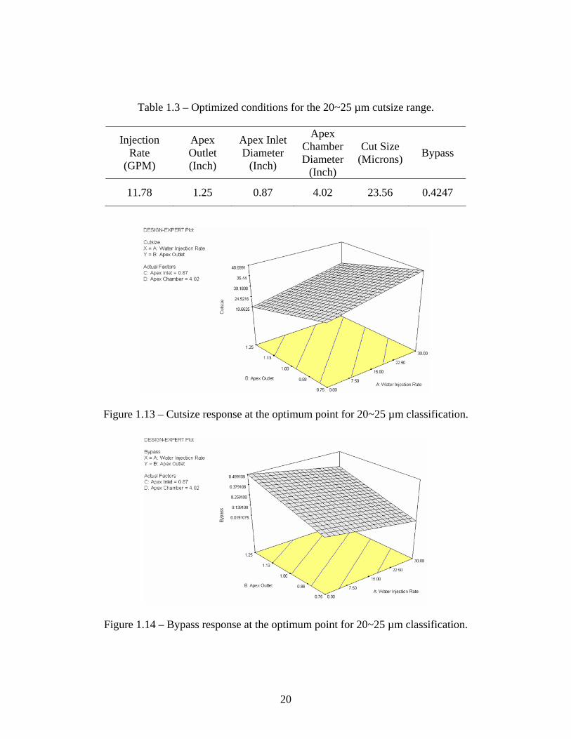
Table 1.3 – Optimized conditions for the 20~25 µm cutsize range.
Injection Rate
(GPM)
Apex Outlet (Inch)
Apex Inlet Diameter
(Inch)
Apex Chamber Diameter
(Inch)
Cut Size (Microns) Bypass
11.78 1.25 0.87 4.02 23.56 0.4247
Figure 1.13 – Cutsize response at the optimum point for 20~25 µm classification.
Figure 1.14 – Bypass response at the optimum point for 20~25 µm classification.

21
Table 1.4 – Optimized conditions for the 25~30 µm cutsize range.
Injection Rate
(GPM)
Apex Outlet (Inch)
Apex Inlet Diameter
(Inch)
Apex Chamber Diameter
(Inch)
Cut Size (Microns) Bypass
13.58 1.03 0.78 4.11 28.98 0.2908
Figure 1.15 – Cutsize response at the optimum point for 25~30 µm classification.
Figure 1.16 – Bypass response at the optimum point for 25~30 µm classification.

22
Table 1.5 – Optimized conditions for the 30~35µm cutsize range.
Injection Rate
(GPM)
Apex Outlet (Inch)
Apex Inlet Diameter
(Inch)
Apex Chamber Diameter
(Inch)
Cut Size (Microns) Bypass
18.50 0.99 0.96 4.24 30.71 0.2416
Figure 1.17 – Cutsize response at the optimum point for 30~35 µm classification.
Figure 1.18 – Bypass response at the optimum point for 30~35 µm classification.

23
Table 1.6 – Optimized conditions for the 35~40 µm cutsize range.
Injection Rate
(GPM)
Apex Outlet (Inch)
Apex Inlet Diameter
(Inch)
Apex Chamber Diameter
(Inch)
Cut Size (Microns) Bypass
25.40 0.85 0.70 4.36 36.09 0.1309
Figure 1.19 – Cutsize response at the optimum point for 35~40 µm classification.
Figure 1.20 – Bypass response at the optimum point for 35~40 µm classification.

24
Table 1.7 – Optimized conditions for the 40~45µm cutsize range.
Injection Rate
(GPM)
Apex Outlet (Inch)
Apex Inlet Diameter
(Inch)
Apex Chamber Diameter
(Inch)
Cut Size (Microns) Bypass
29.77 0.76 0.81 3.94 40.77 0.0231
Figure 1.21 – Cutsize response at the optimum point for 40~45 µm classification.
Figure 1.22 – Bypass response at the optimum point for 40~45 µm classification.

25
1.3.3.1 Optimum Conditions for the 20-25 µm Size Range
The best solution (i.e., combination of water injection rate, apex outlet diameter, apex
inlet diameter and apex chamber diameter) for the 20-25 µm size range is shown in Table 1.8.
For this very small cutsize, it was necessary to employ a low water injection rate and large apex
outlet diameter. As a result, the bypass value was very high at nearly 0.42. These results suggest
that it is not possible to achieve such a small cutsize with this technology unless other
operational parameters not examined in the study are changed (i.e., hydrocyclone geometry, feed
inlet pressure, feed inlet diameter, etc.).
1.3.3.2 Optimum Conditions for the 25-30 µm Size Range
The best solution (i.e., combination of water injection rate, apex outlet diameter, apex
inlet diameter and apex chamber diameter) for the 25-30 µm size range is shown in Table 1.8.
Again, the only way to achieve the small cutsize range was to operate with a relatively low water
injection rate (13.6 GPM) and relatively large apex outlet (1.03 inches). The amount of bypass
Table 1.8 – Summary of optimal conditions needed for different cutsize ranges.
Desired Size Range (Microns
Injection Rate
(GPM)
Apex Outlet (Inch)
Apex Inlet Diameter
(Inch)
Apex Chamber Diameter
(Inch)
Expected Cut Size
(Microns)
Expected Bypass
--
20-25 11.78 1.25 0.87 4.02 23.56 0.4247
25-30 13.58 1.03 0.78 4.11 28.98 0.2908
30-35 18.50 0.99 0.96 4.24 30.71 0.2416
35-40 25.40 0.85 0.70 4.36 36.09 0.1309
40-45 29.77 0.76 0.81 3.94 40.77 0.0231

26
was somewhat lower for this case compared to finer 20-25 µm size range (i.e., 0.29 versus 0.42);
however, the bypass was still relatively large compared to the project goal of achieving bypass
values of less than 0.10-0.15. Nonetheless, these results are considered an improvement over
those typically provided by hydrocyclone deslime circuits that currently operate in the coal
industry. These industrial circuits typically provide cutsizes in the 40-45 µm size range with
bypass values of 0.30-0.35. Thus, the water-injected apex makes it possible to attain a smaller
cutsize with a similar bypass to that of current industrial circuits.
1.3.3.3 Optimum Conditions for the 30-35 µm Size Range
The best solution (i.e., combination of water injection rate, apex outlet diameter, apex
inlet diameter and apex chamber diameter) for the 30-35 µm size range is shown in Table 1.8. In
this case, the somewhat larger cutsize range made it possible to operate with a higher water flow
rate so that the bypass could be reduced below 0.25. This operating range is attractive since it
provides a smaller cutsize that typically found in industrial plants (i.e., normally 40-45 µm) with
significantly less bypass (i.e., normally 30-35%).
1.3.3.4 Optimum Conditions for the 35-40 µm Size Range
The best solution (i.e., combination of water injection rate, apex outlet diameter, apex
inlet diameter and apex chamber diameter) for the 35-40 µm size range is shown in Table 1.8.
The performance obtained in this particular operating range represents a considerable
improvement over that normally achieved in industrial plants. The low bypass of 0.13 for this
case can be attributed to the use of a higher water injection rate (25.4 GPM) and smaller apex
outlet diameter (0.85 inches). Furthermore, the cutsize is smaller (by about 5 µm) than that

27
typically obtained in industrial circuits which utilize conventional hydrocyclones that do not
employ the water injected apex technologies. Therefore, this operating point is considered to be a
very attractive for many of the deslime cyclone circuits that are currently operating in the coal
industry. The use of the new apex washing system would be expected to improve product quality
(due to less bypass) and improve coal recovery (due to the smaller cutsize).
1.3.3.5 Optimum Conditions for the 40-45 µm Size Range
The best solution (i.e., combination of water injection rate, apex outlet diameter, apex
inlet diameter and apex chamber diameter) for the 40-45 µm size range is shown in Table 1.8.
This particular range of cutsize values represents the range that is typically achieved in industrial
deslime cyclone circuits. For this practical range, a very low bypass of just over 0.02 could be
realized by using a water injection flow rate approaching the maximum tested value of 30 GPM.
To achieve the low bypass, a relatively small apex outlet diameter of 0.76 inches had to be used.
The exceptionally low bypass makes this operating point attractive for cases in which the
misplacement of slimes must be avoided in order to make the best possible quality for the final
product. Such applications would include deslime circuits ahead of flotation and product sizing
cyclones installed downstream of fine (100x325 mesh) spirals utilized in some industrial plants.
1.3.3.6 Bypass and Cutsize Correlation Under Optimum Conditions
Several important observations can be made based on the information gathered from the
optimization study. The study indicates that there are no solutions (i.e., no combination of
controllable variables) that provide cutsize values below 20 µm or above 50 µm. This finding
should be expected since none of the cutsize values determined experimentally was found to fall

28
in these ranges. More importantly, the study showed a very strong negative correlation between
cutsize and bypass when operating under optimal conditions. This trend can be seen by the data
plotted in Figure 1.23 for the entire set of optimized test runs conducted in the parametric study.
The Pearson correlation coefficient (R2) value of near unity (R2=0.99) shows an almost
perfect correlation between cutsize and bypass. As such, this plot can be used to estimate the
minimum amount of bypass that can be achieved for a target cutsize. As shown, a reduction in
bypass to 0.1 or lower using the water-injected apex will force the cutsize to increase to
approximately 37 µm or larger. This operating point will likely require a modestly high water
rate (e.g., 26 GPM) and small apex outlet diameter (e.g., 0.8 inches). Likewise, the regression
line shows that a bypass of less than 0.05 dictates a larger cutsize of 40 µm or larger. This
requires a higher water flow rate approaching 30 GPM and relatively small apex approaching
0.75 inches.
Figure 1.23 – Correlation between predicted cutsize and bypass.

29
1.4 Summary and Conclusions
A parametric study was performed to evaluate a new water-injected apex system. The
study indicated that apex outlet diameter and water injection flow rate have the main effect on
minimizing the bypass of ultrafine particles to the underflow. The effects of apex inlet diameter
and apex chamber diameter where not found to be important variables for the range of
dimensions examined in this study. When operated under optimum conditions, the new apex
washing system makes it possible to reduce ultrafine bypass from a typical range of 30~35%
down to approximately 2% when operated within a cutsize range of 40-45 um. A smaller cutsize
range was possible when using less injection water and larger apex outlets, but these changes
tended to rapidly increase the amount of bypass. In fact, a near perfect linear correlation was
observed between cutsize and bypass when operating under the optimum settings of apex
geometry and water flow rate that were needed to minimize bypass.

30
1.5 References
1. K. Heiskanen, 1993. Particle Classification, Chapman & Hall.
2. L. Svarovsky, 1984. Hydrocyclones, Technomic publishing.
3. Stat-Ease Inc., 2002. Design-Expert 6 User’s Guide.
4. M.K. Mohanty, A. Palit and B. Dube, 2002. A comparative evaluation of new fine particle
size separation technologies, Minerals Engineering, Vol. 15, pp. 727–736.
5. M. Frachon and J.J. Cilliers, 1999. A general model for hydrocyclone partition curves,
Chemical Engineering Journal, Vol. 73, pp. 53-59.
6. M.A.Z. Coelho and R.A. Medronho, 2001. A model for performance prediction of
hydrocyclones, Chemical Engineering Journal, Vol. 84, pp. 7–14.
7. Bangxian Wu et al., 2002. A study on advanced concept for fine particle separation,
Experimental Thermal and Fluid Science, Vol. 26, pp. 723–730.
8. F. Concha et al., 1996. Air core and roping in hydrocyclones, Int. J. Miner. Process., Vol. 44-
45, pp. 743-749.
9. R.Q. Honaker et al., 2001. Apex water injection for improved hydrocyclone classification
efficiency, Minerals Engineering, Vol. 14, No. 11, pp. 1445-1457.
10. D.D. Patil and T.C. Rao, 1999. Classification evaluation of water injected hydrocyclone
(Technical note), Minerals Engineering, Vol. 12, No. 12, pp. 1527-1532.
11. A.K. Mukherjee et al., 2003. Effect of increase in feed inlet pressure on feed rate of dense
media cyclone, Int. J. Miner. Process. Vol. 69, pp. 259– 274.
12. Atakan Avci and Irfan Karagoz, 2003. Effects of flow and geometrical parameters on the
collection efficiency in cyclone separators, Aerosol Science, Vol. 34, pp. 937–955.

31
13. G. Vallebuona, A. Casali, G Ferrara, O. Leal and P. Bevilacqua, 1995. Modeling for small
diameter hydrocyclones (Technical note), Minerals Engineering, Vol. 8, No. 3, pp. 321-327.
14. K. Nageswararao, 1999. Normalization of the efficiency curves of hydrocyclone classifiers,
Minerals Engineering, Vol. 12, No. 1, pp. 107-118.
15. T. Neesse, J. Dueck and L. Minkov, 2004. Separation of finest particles in hydrocyclones,
Minerals Engineering, Vol. 17, pp. 689–696.
16. A.J. Lynch and Rao T. C., 1975. Modelling and scale-up of hydrocyclone classifiers,
Proceedings, XI Inter. Miner. Proc. Congress (IMPC), Cagliari, pp. 245-269.
17. L. R. Plitt, 1976. Mathematical Modelling of the hydrocyclone classifier, CIM Bulletin 69,
Vol. 776, pp. 114-123.

32
CHAPTER 2 – MATHEMATICAL SOLUTIONS TO PARITIONING EQUATIONS FOR MULTISTAGE CLASSIFICATION CIRCUITS
2.1 Introduction
2.1.1 Background
Classification processes are used in a wide variety of applications in both the mineral
processing and coal preparation industries. Both static tank and centrifugal separators are used
primarily for the purpose of sorting particles according to size based on differences in settling
rates. In some applications, the classification processes may be used in multistage circuits that
are specifically designed to minimize the misplacement of particles and improve separation
efficiency. For hydraulic classifiers, scavenging circuits can be used to reduce unwanted losses
of coarse particles by retreating the undersize stream using one or more additional stages of
separation. Likewise, cleaning circuits can be used to improve the quality of the coarse product
by retreating the oversize stream in one or more additional units designed to reduce the
inadvertent bypass of fine materials.
In most cases, the natural variations in the physical properties of the feed particles (i.e.,
density, conductivity, magnetic susceptibility, washability) make it difficult to experimentally
determine the extent of the improvement offered by multistage classification circuits. To
overcome this problem, an evaluation of multistage separation circuits was performed in this
study using a mathematical approach. An S-shaped partition function, which has been advocated
for describing hydrocyclone efficiency curves (Lynch and Rao, 1975), was used for all of the
performance calculations conducted in this work. According to this expression, the partition
curve for a separation may be represented by the following exponential transition function:

33
2]exp[]exp[1]exp[
−+−
=αα
αZ
ZP [2.1.1]
where P is probability function to a particular stream, α is the sharpness of separation, and Z
is the ratio of the particle size ( X ) to particle size cutpoint ( 50X ) (i.e., 50/ XXZ = ). It is
generally assumed that the bypass is independent of particle size and equals the water recovery
from the feed to the underflow (oversize) product. This condition assumes that the fraction of the
feed water recovered in the underflow stream carries an equivalent fraction of the feed solids.
Austin and Klimpel (1981) argue that there is no fundamental reason why, in general, this should
be so, and show data where the bypass is clearly not equal to the water recovery. Svarovsky
(1992) and Braun and Bohnet (1990) assume that the bypass equals the fraction of the feed slurry
reporting to the underflow. This assumption is not commonly used, but is a close approximation
to the water recovery at low feed solids concentrations and is more readily measured. The
generalized equation for simulating overall bypass of multistage classification circuits is
obtained by using a following equation:
)1/()( * BpBpPP −−= [2.1.2]
where P and *P represent the corrected and actual probability functions, respectively, and Bp
is the bypass of ultrafine particles to underflow. The actual probability can be obtained by simply
adding water entrainment to corrected probability function.
2.1.2 Linear Circuit Analysis
A comparison of the performance of different configurations of multistage circuits can be
accomplished using a mathematical approach called linear circuit analysis (LCA). This
technique, which was first advocated by Meloy (1983), is one of the most powerful tools for

34
analyzing processing circuits. The LCA approach has been used to improve the performance of
processing circuits in variety of industrial applications (Luttrell et al., 1998). LCA can only be
applied if particle-particle interactions do not influence the probability that a particle will report
to a particular stream, i.e. the partition curve should remain unchanged in each stage of
separation. This assumption is reasonably valid for most classification separators provided that
the machine is functioning within its recommended operating limits (e.g., feed solids content is
not too high). Based on this assumption, circuit analysis will provide not only useful insight into
how unit operations should be configured in a multistage circuit, but also numerical solutions
that predict overall circuit performance.
2.1.3 Objectives
The primary objective of the work outlined in this chapter is to use partition models and
linear circuit analysis to derive analytical expressions that can be used to directly calculate key
indicators that describe the separation performance of multistage classification circuits. For
hydraulic classifiers, some of the specific indicators of interest include particle cutsize, bypass
and separation efficiency. Due to the complexity of the mathematics involved, a commercial
software package known as Mathematica was used to algebraically solve most of the
performance expressions developed in this study. In addition, the accuracy of the analytical
expressions was evaluated by means of direct numerical simulations conducted using iterative
models developed in an Excel spreadsheet format.

35
2.2 Mathematical Software
2.2.1 Mathematica Simulations
Mathematica, a powerful mathematical software package, was utilized to derive general
mathematical equations for the multistage classification circuits and to calculate their overall
particle cutsize and separation efficiency. For the purpose of this study, multistage classification
circuits represent a combination of processing units that include two-stage and three-stage
circuits that incorporate underflow reprocessing, overflow reprocessing, recycle and no recycle.
The “preferred” configurations identified by circuit analysis are limited in this study to three or
less units for practical reasons.
To derive the generalized equations for multistage classification circuits, the combined
probability function for two-stage and three-stage circuits was calculated from the individual
probability function for a single-stage unit using the linear circuit analysis (LCA) methodology.
The combined probability function was entered, simplified and then generalized by the
Mathematica software package. The combined probability function for the multistage circuits
followed the generalized form given by:
),( 50XfP α= [2.2.1]
where P is a probability function (fraction reporting to underflow), α is the separation
sharpness, and 50X is the separation cutsize for each unit. All of the probability equations were
found to be expressed as complex exponential functions, which are non-algebraic and non-linear.
Therefore, to get a solution (i.e., to find α and 50X ) from the combined equations for multistage
circuits, the built-in “FindRoot” function was used in Mathematica. This function can search for
a numerical solution to complex non-algebraic equations by Newton’s method. To find a solution
to an equation of the form 0)( =xf using Newton’s method, the algorithm starts at 0=x , then

36
uses knowledge of the derivative f ′ to take a sequence of steps toward a solution. Each new
calculated point nx that the algorithm tries is found from the previous point 1−nx using the
formula )(/)( 111 −−− ′−= nnnn xfxfxx .
When searching for a solution, the particle cutsize ( 50X ) was represented by a value of
X at which P=0.5. Likewise, the separation sharpness was expressed as follows:
2575
5050 20986.10986.1
XXX
EpX
−==α [2.2.2]
where Ep is the Ecart probable error (another criterion for the separation efficiency) and 25X
and 75X are the particle sizes defined at P=0.25 and P=0.75, respectively. If the values of 25X ,
50X and 75X are known, the particle cutsize and separation sharpness (or Ecart probable error)
can be determined numerically. The formations of the “FindRoot” function that are related
with 25X , 50X and 75X are as follows:
}],{,5.0[ 0XXPFindRoot == [2.2.3]
}],{,25.0[ 0XXPFindRoot == [2.2.4]
}],{,75.0[ 0XXPFindRoot == [2.2.5]
These formations instruct the program to search for an X value that numerically satisfies the
equation “ 75.025.05.0 ororP == ” starting with X=X0.
For the cases involving the probability function with bypass, the following equation was
used to calculate the overall probability function:
)1/()( * BpBpPP −−= [2.2.6]

37
where *P represents the actual probability function (with entrainment), P is the corrected
probability function (no entrainment), and Bp is the ultrafine misplacement to underflow for
each unit. This equation can be rearranged to provide the following expression for *P :
BpPBpP +−= )1(* [2.2.7]
In a manner similar to deriving equations for multistage circuits for overall cutsize and
separation efficiency, the equations for multistage circuits can be generalized for determining the
overall bypass. The combined probability function for multistage circuits that include bypass
followed the generalized form given by:
),,( 50*
LXfP φα= [2.2.8]
where *P is probability function that includes bypass. The termsα , 50X and Lφ represent the
separation sharpness, cutsize, and ultrafine size bypass (misplacement) to underflow for each
unit, respectively. The overall bypass for a specific circuit configuration can be calculated by
setting this probability function ( *P ) equal to 0 within the “FindRoot” function.
Unfortunately, the Mathematica software package had great difficulty in deriving an
equation for the specific particle size of interest due to the complexity of the equations involved.
The form of the exponential expressions constrained Mathematica to solve for X using inverse
functions. This made solutions nearly impossible to obtain. Therefore, in order to derive an
equation for the specific particle size of interest, the term X had to be separated from the other
variables present in the partition expression. The following functions are related with the specific
particle size of interest:
),(50 αPfX = [2.2.9]
),,( *50 LPfX φα= [2.2.10]

38
2.2.2 Excel Simulations
A spreadsheet-based (Microsoft Excel) partitioning model was developed to simulate the
behavior of multistage hydrocyclone circuits. The partitioning performance was calculated using
the following expression (Lynch and Rao, 1975) for the probability function:
21−+
−=
αα
α
eeeP Z
Z
[2.2.11]
where 50/ XXZ = and α is the separation sharpness. An example of the input/output screen from
the Excel simulations of multistage circuits is shown in Figure 2.1. In this display screen, the
units A, B and C represent the primary, secondary and tertiary separators, respectively. The
yellow-shaded input section (A) allows input values for the separation cutsize ( 50X ) and
Figure 2.1 – Multistage classifier simulation using a spreadsheet-based model (example shows three-stage overflow reprocessing circuit with recycle).

39
separation sharpness (α ) to be enter for each unit in the circuit. The interconnection of the
various streams between units A, B and C can be varied using a series of six dropdown menus
(C), which indicate where each of the two products from each separator should report. The
probability to underflow for each unit is calculated from Equation [2.2.11] in the left most
columns (D), (E) and (F). These probabilities are used with the feed tonnage distribution
(yellow-shaded column) to calculate the tonnage entering and exiting each unit A, B and C. The
calculated tonnage values are then used to determine the overall partition probabilities (G) for the
combined circuitry using the simple relationship:
ClassSizeithforTonnageFeedClassSizeithforTonnageUnderflowUnderflowtoobability =Pr [2.2.12]
The partition curves (H) are then obtained by plotting the mean size (C) as a function of the
combined partition values (G), as well as the individual partition values (D), (E) and (F) for each
unit. The overall cutsize and separation efficiency for the multistage circuit is reported as a
summary output (B).
The predictions obtained from the theoretical equations derived from Mathematica for
determining the circuit partition factors were found to be equivalent to the simulation results
obtained from the Excel simulation spreadsheet. The exact agreement between the Mathematica
and Excel partition values verifies that, for any particle cutsize and separation sharpness, a circuit
partition curve can be calculated analytically from the probabilities without the need to know the
feed size distribution. This finding is extremely important since most investigators do not realize
that simulations based on partitioning probabilities are independent of the physical properties of
the feed stream. In other words, the same cutsize and efficiency will be obtained from the
simulations routines regardless of what feed size distribution is entered. Only the product size
distributions will change in response to changes in the feed size distribution.

40
2.3 Results
2.3.1 Underflow Reprocessing Circuit Without Recycle
2.3.1.1 Two-Stage Circuit Analysis
The underlying principle of LCA is that all particles that enter a separator as feed ( F ) are
selected to report to either the concentrate ( C ) or tailing ( T ) streams by a dimensionless
probability function ( P ). This can be mathematically described for a two-stage underflow
reprocessing circuit without recycle as shown in Figure 2.2. In this case, 0P and 1P represent the
partition probabilities for the primary and secondary units, respectively. By simple algebraic
calculation, the oversize-to-feed ratio ( underTPFT ,= ) for this particular circuit can be
represented as:
10, PPP underT = [2.3.1]
This equation can be easily expanded using a transition function to quantify the separation
probability that occurs for each separator. If a standard classification model is used (Lynch and
Rao, 1977), then the partition for each unit in the circuit can be calculated using:
Figure 2.2 – Schematic of a two-stage underflow reprocessing circuit without recycle.

41
2
1−+
−= αα
α
eeeP Z
Z
[2.3.2]
where P is the partition factor, α is a sharpness value and Z represent the normalized size
given by 50XX . By substituting the partition function given by Equation [2.3.2] into the
separation probabilities represented in Equation [2.3.1], the overall partition expression for this
circuit now becomes:
PT =Heα0 Z0 −1L Heα1 Z1 − 1L
Heα0 + eα0 Z0 −2L Heα1 + eα1 Z1 − 2L [2.3.3]
where 0α and 1α are the sharpness values and 0Z and 1Z are the normalized size for the primary
and secondary separators, respectively. This equation represents the combined partitioning
probability for a two-stage underflow reprocessing circuit without any recycle streams.
To check the validity of Equation [2.3.3], a comparison was made between the analytical
solution and a simulation results obtained using the spreadsheet program described previously.
The partitioning data selected for use in this validation procedure are shown in Figure 2.3. For
each technique, the primary and secondary separators were set to make a respective cutsize of
150 and 106 mµ . The separation sharpness values for the primary and secondary units were also
set at different values of 2.748 and 3.661, respectively. By substituting these values into the
Equation [2.3.3], the overall partition expression for this circuit becomes:
PT =He0.01831X − 1L He0.0345X − 1L
H13.588+ e0.01831 XL H36.939+e0.0345 XL [2.3.4]
A comparison of the partitioning results obtained using this expression and those obtained from
the Excel simulations are summarized in Table 2.1. As should be expected, the Mathematica
solution for determining circuit partition factors is mathematically equivalent to the Excel
simulation (which utilized feed properties). The good agreement between the Mathematica and

42
Excel partition values verifies that for any particle cutsize, a circuit partition value can be
calculated. This also indicates that important size values, such as 25X , 50X , and 75X , can be
back-calculated from Equation [2.3.4] by varying X until the desired values of P are found.
More importantly, important performance indicators, such as the separation sharpness (α ) and
cutsize ( 50X ), can be determined for the entire circuit completely independent of feed properties.
As discussed previously, Mathematica can be used to perform the calculations required to
determine the important performance indicators for the two-stage circuit. In trying to find
solution to this equation, Newton’s method was used to determine the values of X needed to
identify the cutsize ( 50X ) and calculate the separation sharpness (α ). To accomplish this goal,
the appropriate X values were determined using the “FindRoot” function which searches for a
Figure 2.3 – Example of the partitioning response of the two-stage circuit underflow reprocessing circuit without recycle.

43
numerical solution to each expression using Newton’s method. The form of the “FindRoot”
function used to calculate these values are as follows:
}],{,5.0[ 0XXPFindRoot == [2.3.6]
}],{,25.0[ 0XXPFindRoot == [2.3.7]
}],{,75.0[ 0XXPFindRoot == [2.3.8]
The statement represented by Equation [2.3.6] instructs Mathematica to search X values for a
numerical solution to the equation “ 5.0=P ” starting with 0XX = . Using this approach, the
cutsize and separation sharpness for the total two-stage circuit was found to be 164.54 mµ and
3.971, respectively. These exact values were calculated totally independent of the feed properties
using the features readily available within Mathematica. The analytical solution also indicates
that the use of this particular two-stage circuit substantially increases the cutsize when compared
to the cutsize values set for either of the single unit operations.
Table 2.1 – Comparison of Mathematica and Excel determined partition factors for the two-stage underflow reprocessing circuit without recycle.
Particle Size
(mm) Mathematica
Partition Factor Excel
Partition Factor 0.714 0.505 0.357 0.252 0.18 0.126 0.089 0.063 0.049 0..041 0.028 0.010
1.000 0.999 0.978 0.861 0.579 0.262 0.089 0.031 0.017 0.012 0.006 0.003
1.000 0.999 0.978 0.861 0.579 0.262 0.089 0.031 0.017 0.012 0.006 0.003

44
2.3.1.2 Three-Stage Circuit Analysis
The approach described previously for the two-stage circuit was again applied to provide
an analytical partitioning expression for a three-stage underflow reprocessing circuit without
recycle. In this case, 0P , 1P and 2P are the dimensionless probability functions that select
particles to report to a given stream for the primary, secondary and tertiary separators,
respectively. As shown in Figure 2.4, the overall refuse-to-feed ratio ( underTPFT ,= ) for this
circuit can be represented as:
210, PPPP underT = [2.3.9]
By substituting Equation [2.3.2] into this expression, the overall partition function for this three-
stage circuit becomes:
PT =Heα0 Z0 − 1L Heα1 Z1 −1L Heα2 Z2 − 1L
Heα0 + eα0 Z0 − 2L Heα1 + eα1 Z1 − 2L Heα2 + eα2 Z2 − 2L [2.3.10]
Figure 2.4 – Schematic of a three-stage underflow reprocessing circuit without recycle.

45
In this case, the primary, secondary and tertiary separators were set to make separations at the
particle cutsize of 150, 106 and 75 mµ with separation sharpness values of 2.748, 3.661 and
3.663, respectively. The partition values calculated from Mathematica and Excel were again
found to exactly agree for this circuit. The cutsize and separation sharpness for total circuit was
found to be 165.55 mµ and 4.135, respectively. Once again, the analytical solution shows that
the cutsize for the combined circuit is larger than that obtained for either of the single unit
operations.
3.3.2 Underflow Reprocessing Circuit With Recycle
2.3.2.1 Two-Stage Circuit Analysis
The approach described above can also be used to evaluate the effects of recycle streams
on the performance of multistage circuits. This type of assessment is traditionally much more
difficult to perform with standard simulation routines since it requires several iterations to find a
stable solution. However, no such problem exists for analytical solutions obtained using linear
circuit analysis.
Consider the two-stage underflow reprocessing circuit with recycle shown in Figure 2.5.
Once again, 0P and 1P represent the dimensionless probability functions that select particles to
report to a given stream. By simple algebraic substitution, the overall oversize-to-feed ratio
( underTPFT ,= ) for this particular circuit can be calculated as:
)1( 10010, PPPPPP underT +−= [2.3.11]
By substituting Equation [2.3.2] into this expression, the overall partition expression for this
circuit becomes:

46
PT =H−1+ eα0 Z0L H−1+ eα1 Z1L
3− 2eα0 − eα0 Z0 − eα1 − 2eα1 Z1 + eα0+α1 + eα0+ α1 Z1 + eα0 Z0+α1 Z1 [2.3.12]
To check the validity of this expression, a comparative solution was again obtained from the
Excel spreadsheet simulation routine. In this case, the primary, secondary and tertiary separators
were set to make a cutsize of 150, 106 and 75 mµ with separation sharpness values of 2.748,
3.661 and 3.663, respectively. As expected, both the Mathematica and Excel partition values
were in perfect agreement for this three-stage circuit. The cutsize and separation sharpness for
total circuit was found to be 158.30 mµ and 3.717, respectively. In this case, the increase in
cutsize created by the use of a two-stage circuit is less with a recycle stream than without a
recycle stream (i.e., 158.30 versus 164.54 mµ ).
2.3.2.2 Three-Stage Circuit Analysis
In this case, an analytical solution to the partitioning performance of a three-stage circuit
with recycle was derived using linear circuit analysis. A schematic of the three-stage circuit is
Figure 2.5 – Schematic of a two-stage underflow reprocessing circuit with recycle.
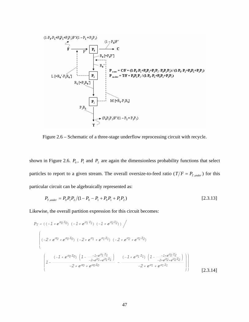
47
shown in Figure 2.6. 0P , 1P and 2P are again the dimensionless probability functions that select
particles to report to a given stream. The overall oversize-to-feed ratio ( underTPFT ,= ) for this
particular circuit can be algebraically represented as:
)1( 211010210, PPPPPPPPPP underT ++−−= [2.3.13]
Likewise, the overall partition expression for this circuit becomes:
PT = HH−1+ α0 Z0L H−1+ α1 Z1L H−1+ α2 Z2LL ì
i
k
jjjjjjjjH−2+ α0 + α0 Z0L H−2+ α1 + α1 Z1L H−2+ α2 + α2 Z2L
i
k
jjjjjjjj1−
H−1+ α0 Z0L J1− −1+ α1 Z1−2+ α1+ α1 Z1
N
−2+ α0 + α0 Z0−H−1+ α1 Z1L J1− −1+ α2 Z2
−2+ α2+ α2 Z2N
−2+ α1 + α1 Z1
y
{
zzzzzzzz
y
{
zzzzzzzz [2.3.14]
Figure 2.6 – Schematic of a three-stage underflow reprocessing circuit with recycle.

48
when substituting Equation [2.3.2] into the expression derived from linear circuit analysis. For
verification purposes, the primary, secondary and tertiary separator were set to make separations
at cutsize values of 150, 106 and 75 mµ with separation sharpness values of 2.748, 3.661 and
3.663, respectively. The Mathematica and Excel partition values were again found to be
consistent for this circuit, indicating that the analytical solution was indeed accurate. The cutsize
and separation sharpness for total circuit were found to be 158.32 mµ and 3.737, respectively,
based on the input values selected for the individual units. It is important to notice that cutsize of
158.32 mµ obtained with this three-stage circuit with recycle streams was substantially smaller
than the cutsize of 165.55 mµ obtained for the three-stage circuit without recycle. Thus, the use
of recycle streams suppresses the impact of increasing cutsize for multistage circuits in which the
underflow stream is retreated to reduce bypass.
2.3.3 Overflow Reprocessing Circuit Without Recycle
2.3.3.1 Two-Stage Circuit Analysis
Several series of calculations were also performed to quantify the partitioning behavior of
Figure 2.7 – Schematic of a two-stage overflow reprocessing circuit without recycle.

49
circuits in which one or more of the overflow (undersize) streams were reprocessed. In the first
example, a two-stage overflow reprocessing circuit without recycle was evaluated as shown in
Figure 2.7. For this configuration, the overall oversize-to-feed ratio ( underTPFT ,= ) is:
1010, PPPPP underT −+= [2.3.15]
Substituting Equation [2.3.2] into this expression gives the overall partition expression as:
PT =−1+ α0 Z0
−2+ α0 + α0 Z0+H−1+ α1 Z1L J1− −1+ α0Z0
−2+ α0+ α0 Z0N
−2+ α1 + α1 Z1 [2.3.16]
Both the Mathematica and Excel solutions for the partition values were identical, indicating
again that the analytical solution was accurate. In this case, the primary and secondary separators
were set to provide respective cutsize values of 150 and 106 mµ and respective separation
sharpness values of 2.748 and 3.661. Based on these input values, the cutsize and separation
sharpness for the total circuit was found to be 87.06 mµ and 2.805, respectively. In this case, the
use of a two-stage circuit to retreat the undersize product reduced the overall cutsize compared to
the cutsize .
2.3.3.2 Three-Stage Circuit Analysis
Figure 2.8 shows the layout for a three-stage overflow reprocessing circuit without
recycle. The overall oversize-to-feed ratio ( underTPFT ,= ) for this circuit can be calculated from
linear circuit analysis as:
210212010210, PPPPPPPPPPPPP underT +−−−++= [2.3.17]
Similar to the previous section, the overall partition expression for this circuit becomes:

50
PT =−1+ α0 Z0
−2+ α0 + α0 Z0+H−1+ α1 Z1L J1− −1+ α0Z0
−2+ α0+ α0 Z0N
−2+ α1 + α1 Z1+
H−1+ α2 Z2L J1− −1+ α0 Z0−2+ α0+ α0 Z0
N J1− −1+ α1 Z1−2+ α1+ α1 Z1
N
−2+ α2 + α2 Z2 [2.3.18]
The primary, secondary and tertiary separators were set to make separations at the particle size
cut-point of the 150, 106 and 75 mµ with sharpness values of 2.748, 3.661 and 3.663,
respectively. The Mathematica and Excel partition values are also consistent in this circuit. The
cutsize and separation sharpness values for total circuit were found to be 61.56 mµ and 3.449,
respectively. Notice that reprocessing of the overflow by three stages of operations substantially
reduced the cutsize compared to the values entered for the individual unit operations.
2.3.4 Overflow Reprocessing Circuit With Recycle
2.3.4.1 Two-Stage Circuit Analysis
This particular analysis examined a two stage overflow reprocessing circuit with recycle.
A schematic of the circuit is shown in Figure 2.9. The overall refuse-to-feed ratio and
partitioning expression for this circuit is given by:
Figure 2.8 – Schematic of a three-stage overflow reprocessing circuit without recycle.

51
)1( 1010, PPPPP underT +−= [2.3.19]
PT =−1+ α0Z0
H−2+ α0 + α0 Z0Li
k
jjjjjjj1−
I−1+ α1 Z1Mikjj1− −1+ α0 Z0
−2+ α0+ α0 Z0y{zz
−2+ α1+ α1 Z1
y
{
zzzzzzz [2.3.20]
The Mathematica and Excel solutions were again found to provide identical partition values for
this circuit. For validation purposes, the primary, secondary and tertiary separator were set to
make separations at cutsize values of 150 and 106 mµ with sharpness values of 2.748 and 3.661,
respectively. Based on these values, the cutsize and separation sharpness for total circuit was
found to be 109.12 mµ and 3.862, respectively. When compared to the two-stage overflow
reprocessing circuit without recycle, the recycle configuration provided a substantially smaller
cutsize (i.e., 87.06 vs. 109.12 mµ ).
Figure 2.9 – Schematic of a two-stage overflow reprocessing circuit with recycle.

52
2.3.4.2 Three-Stage Circuit Analysis
The last circuit examined in detail in this study was a three-stage overflow reprocessing
circuit with recycle. The layout of units for this particular circuit is shown in Figure 2.10. Based
on the probability analyses for this circuit, the overall oversize-to-feed ratio ( underTPFT ,= ) was
found to be given by:
)1()( 211021210200, PPPPPPPPPPPPP underT ++−−+−= [2.3.21]
Once again, by substituting Equation [2.3.2] into this expression, the overall partition expression
for this circuit can be directly calculated as:
PT =
H−1+ α0 Z0Li
k
jjjjjjj1−
I−1+ α2 Z2Mikjj1− −1+ α1Z1
−2+ α1+ α1 Z1y{zz
−2+ α2+ α2 Z2
y
{
zzzzzzz
H−2+ α0 + α0 Z0Li
k
jjjjjjj1−
I−1+ α1 Z1Mikjj1− −1+ α0 Z0
−2+ α0+ α0 Z0y{zz
−2+ α1+ α1 Z1−
I−1+ α2 Z2Mikjj1− −1+ α1 Z1
−2+ α1+ α1 Z1y{zz
−2+ α2+ α2 Z2
y
{
zzzzzzz [2.3.22]
The primary, secondary and tertiary separator were set to make separations at cutsize values of
Figure 2.10 – Schematic of a three-stage overflow reprocessing circuit with recycle.

53
150, 106 and 75 mµ ) with separation sharpness values of 2.748, 3.661 and 3.663, respectively.
The Mathematica and Excel partition values were again identical, providing cutsize and
sharpness values for total circuit of 88.79 mµ and 6.167, respectively.

54
2.4 Generalized Partitioning Expressions
2.4.1 Underflow Reprocessing Circuit Without Recycle
The generic configurations of underflow reprocessing circuits without recycle are shown
in Figure 2.11. The probability functions for each circuit can be readily calculated by linear
circuit analysis. The single-stage probability can be expressed as follows:
0PPT = [2.4.1]
The two-stage probability can be expressed as follows:
10 PPPT = [2.4.2]
The three-stage probability can be expressed as follows:
210 PPPPT = [2.4.3]
From these expressions, a generalized equation of this specific type of circuit can be obtained as
follows:
Figure 2.11 – Generic configurations of underflow reprocessing circuits without recycle.

55
PT = ‰N=1
nPN−1
[2.4.4]
where n is number of classification separators in the circuit. When considering bypass, the
generalized equation for this circuit can be obtained as:
PT∗ = ‰
N=1
nPN−1
∗
[2.4.5]
where the probability ( *P ) for single-stage, two-stage and three-stage units can be expressed as:
BpPBpP +−= )1(* [2.4.6]
As indicated previously, the respective values of P and *P represent the corrected and actual
probability functions for the circuit and Bp represents the bypass of fine particles to the
underflow stream. The probability functions ( P ) for each separator can be estimated based on
the empirical formula (Lynch and Rao, 1977):
21−+
−= αα
α
eeeP Z
Z
[2.4.7]
where α is the separation sharpness and Z=X/X50 is the normalized particle size, i.e., the ratio of
the actual particle size of interest (X) divided by the cutsize (X50).
2.4.2 Underflow Reprocessing Circuit With Recycle
Generic configurations of underflow reprocessing circuits without recycle are shown in
Figure 2.12. The probability functions calculated by linear circuit analysis for each circuit are as
follows. The single-stage probability can be expressed as follows:
0PPT = [2.4.8]
The two-stage probability can be expressed as follows:

56
PT =P0 P1
1− P0 + P0 P1 [2.4.9]
This equation can be further simplified as follows:
PT =
P0 P1
1− P0 H1− P1L [2.4.10]
The three-stage probability can be expressed as follows:
PT =P0 P1 P2
1− P0 − P1 + P0 P1 + P1 P2 [2.4.11]
Likewise, this equation can be further simplified as follows:
PT =P0 P1 P2
1− P0 H1− P1L − P1H1− P2L [2.4.12]
From the functional forms of these equations, a generalized equation for this specific type of
circuit can be obtained as follows:
Figure 2.12 – Generic configurations of underflow reprocessing circuits with recycle.

57
PT =i
kjjjj‰
N=1
nPN−1
y
{zzzz ì
i
kjjjj1− ‚
N=2
nPN−2 H1− PN−1L
y
{zzzz
[2.4.13]
where n is number of classification separators in the circuit. When considering bypass, the
generalized equation for this specific circuit is simply modified to:
PT∗ =
i
kjjjj‰
N=1
nPN−1
∗ y
{zzzz ì
i
kjjjj1− ‚
N=2
nPN−2
∗ H1− PN−1∗ L
y
{zzzz
[2.4.14]
2.4.3 Overflow Reprocessing Circuit Without Recycle
Generic configurations of underflow reprocessing circuits without recycle are shown in
Figure 2.13. From linear circuit analysis, the probability for a single stage circuit can be
expressed as follows:
0PPT = [2.4.15]
The partitioning probability for a two-stage circuit can be expressed as follows:
PT = P0+ P1 − P0 P1 [2.4.16]
This equation can be further simplified to:
Figure 2.13 – Generic configurations of overflow reprocessing circuits without recycle.

58
PT = P0 + H1− P0L P1 [2.4.17]
Likewise, the partitioning probability for a three-stage can be expressed as follows:
PT = P0 + P1 + P2 − P0 P1 − P0 P2 − P1 P2 + P0 P1 P2 [2.4.18]
This equation can be further simplified to:
PT = P0 + H1 − P0L P1 +H1 − P0L H1− P1L P2 [2.4.19]
From these equations, a generalized expression for this specific type of circuit incorporating n
unit operations can be obtained by inspection. The partitioning probability for circuits without
bypass is given as:
PT = P0 + Pn−1 i
k
jjjjjj„N=2
n i
kjjjj‰
N=2
nH1 − PN−2L
y
{zzzz − „
N=3
n i
kjjjj‰
N=2
nH1 − PN−2L
y
{zzzzy
{
zzzzzz + Pn−2 ‚N=3
nH1 − PN−3L
[2.4.20]
while the partitioning probability for circuits with bypass is given as:
PT∗ = P0
∗ + Pn−1∗
i
k
jjjjjj„N=2
n i
kjjjj‰
N=2
nH1− PN−2
∗ Ly
{zzzz − „
N=3
n i
kjjjj‰
N=2
nH1− PN−2
∗ Ly
{zzzzy
{
zzzzzz + Pn−2∗ ‚
N=3
nH1− PN−3
∗ L [2.4.21]
The values of P and *P in these expression represent the partitioning probabilities for each unit
operation with and without bypass, respectively.
2.4.4 Overflow Reprocessing Circuit With Recycle
Generic configurations of underflow reprocessing circuit without recycle are as shown in
Figure 2.14. The probability functions for the single-, two- and three-stage circuits can be
mathematically represented as follows. The single-stage probability can be expressed as:
0PPT = [2.4.22]
The two-stage probability, which can be expressed as:
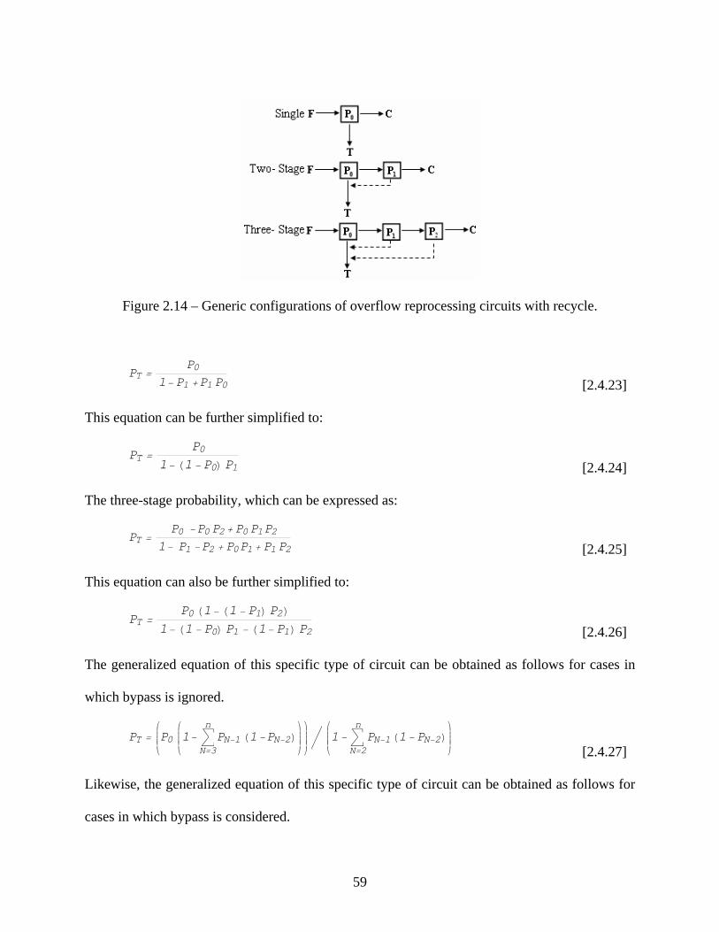
59
PT =P0
1− P1 + P1 P0 [2.4.23]
This equation can be further simplified to:
PT =
P0
1− H1− P0L P1 [2.4.24]
The three-stage probability, which can be expressed as:
PT =P0 − P0 P2 + P0 P1P2
1− P1 − P2 + P0P1 + P1 P2 [2.4.25]
This equation can also be further simplified to:
PT =P0 H1− H1− P1L P2L
1− H1− P0L P1 − H1− P1L P2 [2.4.26]
The generalized equation of this specific type of circuit can be obtained as follows for cases in
which bypass is ignored.
PT =i
kjjjjP0
i
kjjjj1− ‚
N=3
nPN−1 H1− PN−2L
y
{zzzzy
{zzzz ì
i
kjjjj1− ‚
N=2
nPN−1 H1− PN−2L
y
{zzzz
[2.4.27]
Likewise, the generalized equation of this specific type of circuit can be obtained as follows for
cases in which bypass is considered.
Figure 2.14 – Generic configurations of overflow reprocessing circuits with recycle.

60
PT∗ =
i
kjjjjP0
∗ i
kjjjj1− ‚
N=3
nPN−1
∗ H1−PN−2∗ L
y
{zzzzy
{zzzz ì
i
kjjjj1− ‚
N=2
nPN−1
∗ H1− PN−2∗ L
y
{zzzz
[2.4.28]
In both these expressions, n represents the number of classification separators in each circuit.

61
2.5 Summary and Conclusions
Linear circuit analysis was combined with an empirical model of particle classification to
derive analytical expressions that describe the partitioning performance of multistage circuits.
Due to the complexity of the mathematical functions, a software package known as Mathematica
was used to perform the required computations dictated by linear circuit analysis. Although
Mathematica had great difficulty in deriving analytical equations for a specific particle size of
interest, this powerful tool still provided a convenient platform for searching for solutions via
Newton’s method. In addition, this approach provided useful insight into how unit operations
should be configured in multistage circuits to reduce bypass and manipulate cutsize.
The partitioning data derived from Mathematica provided values that were identical to
those obtained from simulations performed using a traditional partition model developed using
an Excel spreadsheet. The perfect agreement between these two diverse approaches verifies that
circuit partition values can be accurately calculated using a direct analytical approach and
without the need for simulation. As such, critical values of particle size (e.g., 25X , 50X and
75X ) that are important in describing the performance of classification units, can be back-
calculated from the partitioning equations derived by linear circuit analysis. This ability confirms
that the two most important performance indicators, i.e., cutsize ( 50X ) and separation sharpness
(α ), can be determined for the combined circuit completely independent of feed properties.
The analytical approach outlined in this study also made it possible to derive generic
expressions for partitioning probability for generalized circuits that reprocess either overflow
(undersize) or underflow (oversize). These expressions indicate that classification performance is
indeed improved through the proper application of multistage circuits and that recycling of

62
secondary streams can in many cases effectively minimize cutsize changes that inadvertently
occur in multistage processing circuits.

63
2.6 References
1. A.J. Lynch and T.C. Rao, “Modeling and Scale-Up of Hydrocyclone Classifiers.” No.9, 11th
Inter Mineral Processing Congress, Cagliari, Italy, April 21-26, 1975.
2. L.G. Austin and R.R. Klimpel, 1981. An improved method for analyzing classifier data,
Powder Technol., Vol. 29, pp. 277–281.
3. L. Svarovsky, Hydrocyclones, Holt, Rinehart and Winston, London, 1992, pp. 198.
4. T. Braun and M. Bohnet, 1990. Influence of feed solid concentration on the performance of
hydrocyclones, Chem. Eng. Technol., Vol. 13, pp. 15–20.
5. T. P. Meloy, 1983. Analysis and optimization of mineral processing and coal-cleaning
circuits–circuit analysis, International Journal of Mineral Processing, Vol. 10, pp. 61-80.
6. G. H. Luttrell, J. N. Kohmuench, F. L. Sranley, and G. D. Trump, 1998. Improving spiral
performance using circuit analysis, Minerals & Metallurgical Processing, Vol. 15, pp.16-21.
7. G. H. Luttrell, J. N. Kohmuench, and M. J. Mankosa, 2004. Optimization of magnetic
separator circuit configurations, Minerals & Metallurgical Processing, Vol. 21, pp. 153–157.
8. J. J. Cilliers and M. Franchon, 1999. A general model for hydrocyclone partition curve,
Chemical Engineering Journal, Vol. 73, pp. 53–59.
9. B. Firth and M. O’Brien, 2003. Hydrocyclone Circuits, Coal Preparation, Vol. 23, pp. 167–
183.
10. L. R. Plitt, 1976. A mathematical model of the hydrocyclone classifier, CIM Bull., pp. 114–
122.

64
APPENDIX I

65
Detailed Parametric Test Matrix
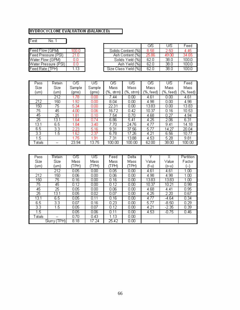
66

67

68

69

70

71

72

73

74

75

76

77

78

79

80

81

82

83

84

85

86

87

88

89

90

91

92

93

94

95

96

97

98

99
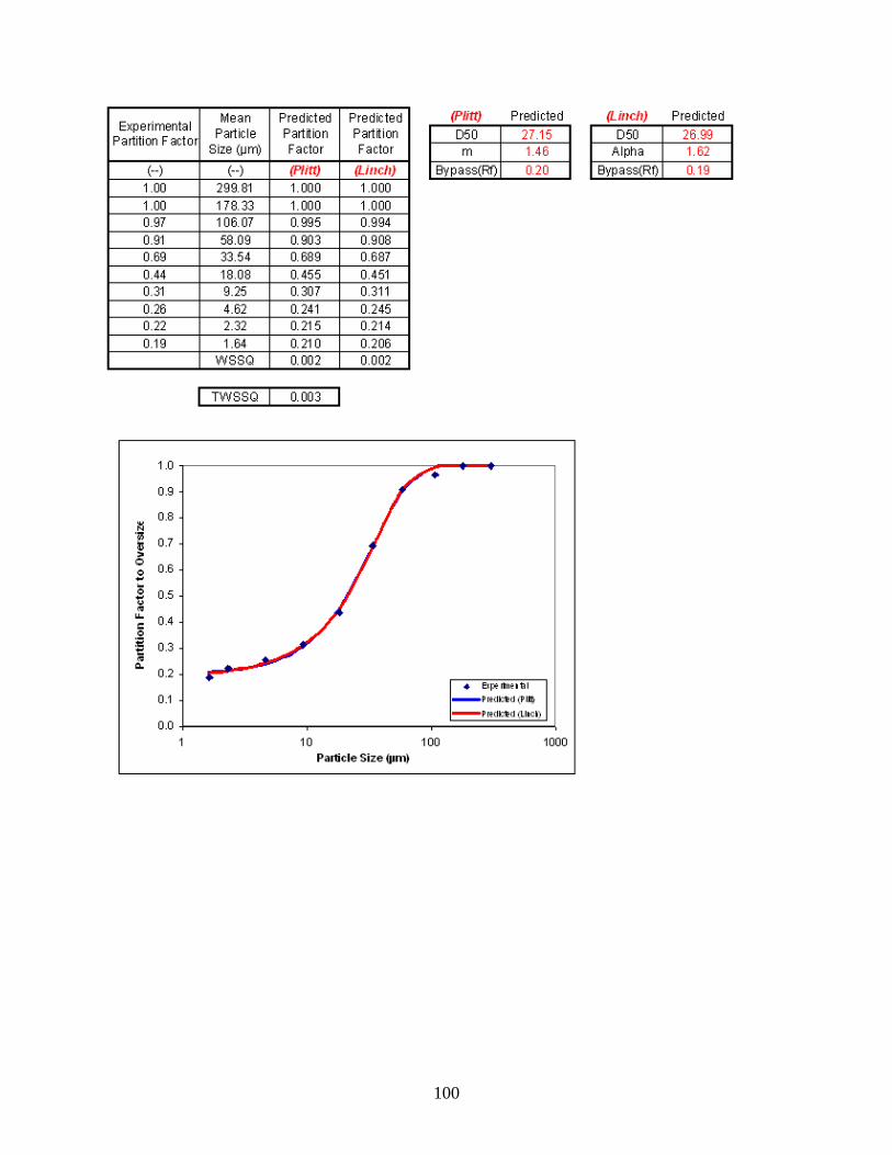
100

101

102

103

104

105

106

107

108

109

110

111

112

113
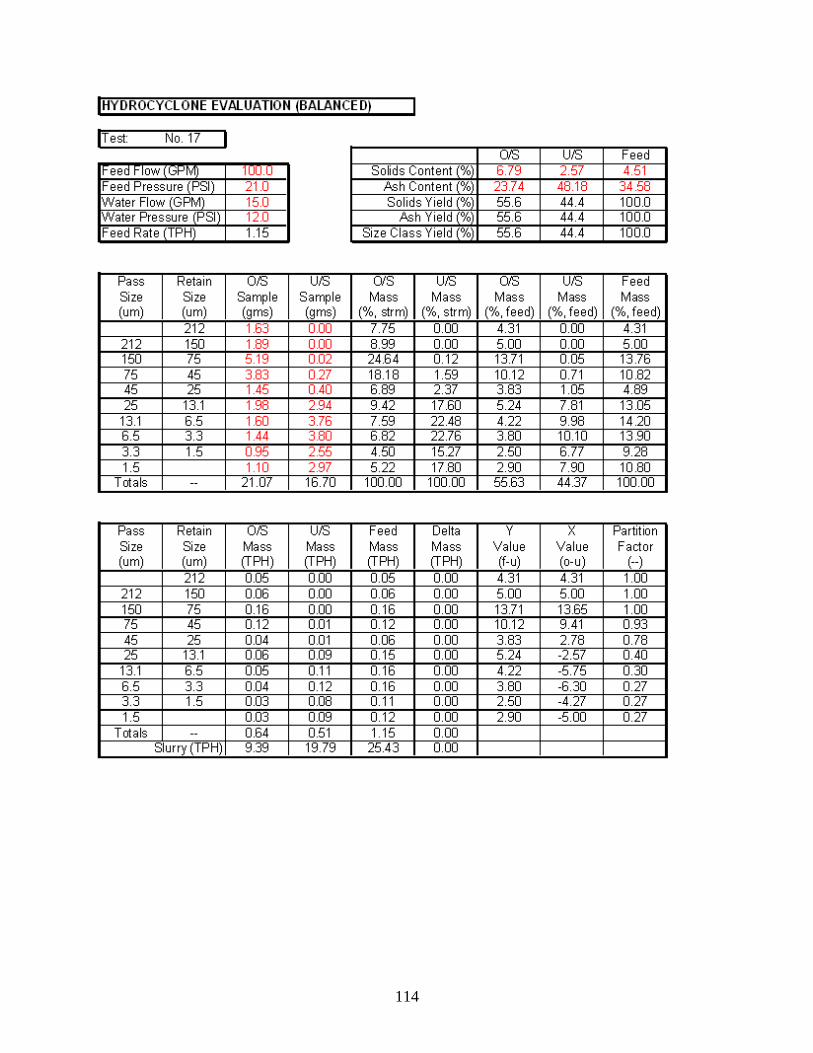
114

115

116

117

118

119

120

121
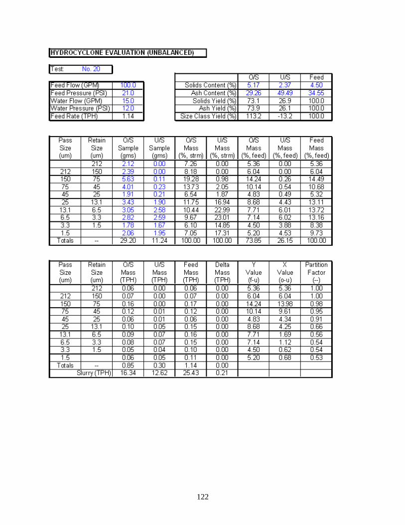
122

123

124

125

126

127

128

129

130

131

132

133

134

135

136

137

138

139

140

141

142

143

144

145

146

147

148

149

150

151

152

153

154

155

156

157

158
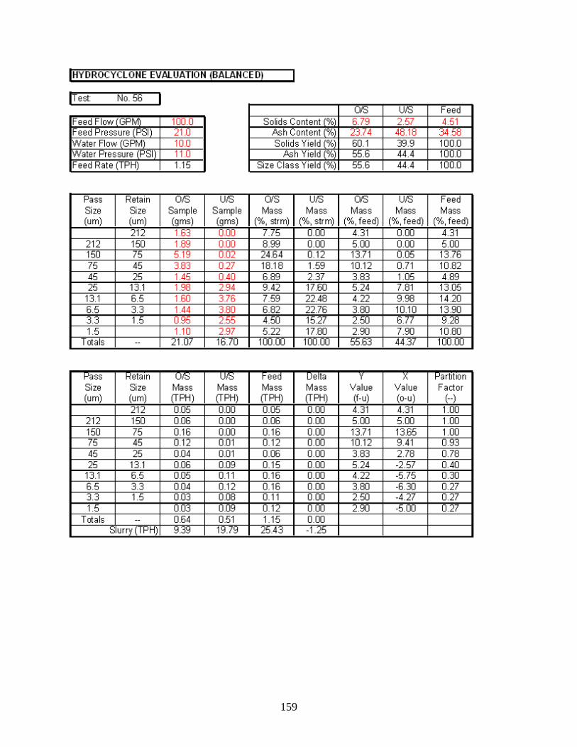
159

160

161

162
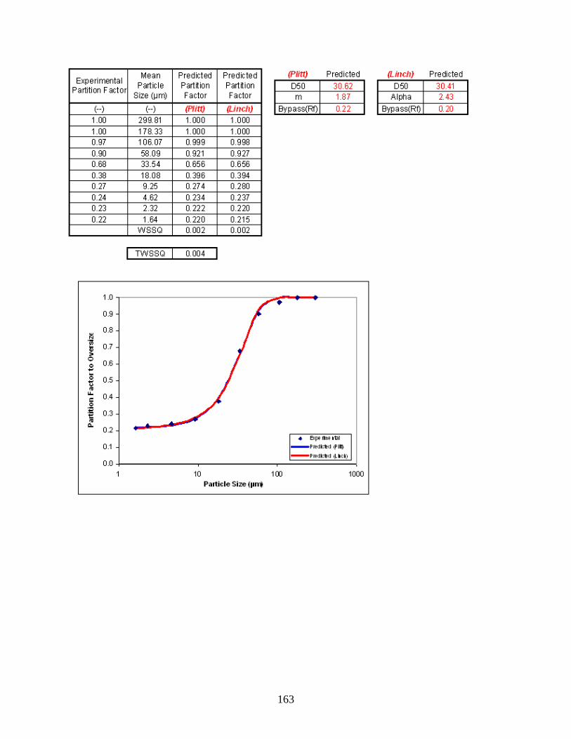
163
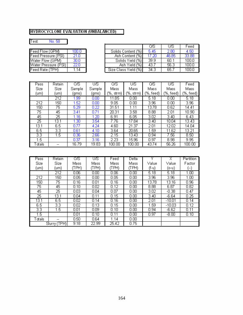
164

165

166

167
Tabular Summary of Parametric Test Results

168
VITA
Dongcheol Shin was born in Pusan, South Korea on the 19th day of September, 1972. He
graduated from Haksung High School in the winter of 1991. The following spring, he was
granted admission to Dong-A university, where he went on to gain a Bachelor of Engineering
degree in Mineral and Mining Engineering. During his time as an undergraduate, he was
involved in some projects of ventilation and rock mechanics. In addition, he had served Korean
government at infantry military for 2 years. After graduating in the winter of 1998, he remained
at Dong-A university to pursue a Master of Engineering degree in Mineral and Mining
Engineering with an emphasis in development of environmental material for a waste water
treatment. He completed his degree in the winter of 2000 and he had worked at the same
university as Business Incubator Manager for 1 year. He learned what principal of economics is
in detail from this job. His life of Mineral Processing was beginning after this job. He got chance
to get an internship to be considered mineral processing industry from Korean Institute of
Geoscience and Mineral Resources (KIGAM), the only government research center of a mineral
processing. After internship, he was granted admission to Virginia Polytechnic Institute and State
University (Virginia Tech) to pursue a Master of Science degree in Mineral and Mining
Engineering with an emphasis in a mineral processing. Upon completion of his thesis of Master
of Science, Dongcheol is preparing to get a job offer in mining industry and will begin his
professional career as a process engineer in the United States.