evaluation of monte-carlo tree search for xiangqi
TRANSCRIPT

Computer ScienceDepartment
Artificial Intelligence andMachine Learning Lab
Evaluation of Monte-Carlo Tree
Search for XiangqiBachelor thesis by Maximilian LangerDate of submission: April 19, 2021
1. Review: Prof. Dr. Kristian Kersting2. Review: Johannes CzechDarmstadt

Erklärung zur Abschlussarbeit
gemäß ğ22 Abs. 7 und ğ23 Abs. 7 APB der TU Darmstadt
Hiermit versichere ich, Maximilian Langer, die vorliegende bachelor thesis ohne Hilfe Dritter und nur mit den
angegebenen Quellen und Hilfsmitteln angefertigt zu haben. Alle Stellen, die Quellen entnommen wurden,
sind als solche kenntlich gemacht worden. Diese Arbeit hat in gleicher oder ąhnlicher Form noch keiner
Prüfungsbehörde vorgelegen.
Mir ist bekannt, dass im Fall eines Plagiats (§38 Abs. 2 APB) ein Tąuschungsversuch vorliegt, der dazu führt,
dass die Arbeit mit 5,0 bewertet und damit ein Prüfungsversuch verbraucht wird. Abschlussarbeiten dürfen
nur einmal wiederholt werden.
Bei der abgegebenen Thesis stimmen die schriftliche und die zur Archivierung eingereichte elektronische
Fassung gemąß §23 Abs. 7 APB überein.
Bei einer Thesis des Fachbereichs Architektur entspricht die eingereichte elektronische Fassung dem vorgestell-
ten Modell und den vorgelegten Pląnen.
Darmstadt, April 19, 2021
M. Langer
2

Abstract
In this thesis we evaluate training deep neural networks on human data in chinese chess and combining
them with Monte-Carlo Tree Search. No later than after DeepMinds’ publication of the AlphaGo algorithm,
this cooperation of neural networks and Monte-Carlo Tree Search has proven very successful. Choosing the
networks’ architecture represents a key aspect for the achievable performance. We inspect two architectures,
namely RISEv2 mobile and RISEv3 mobile, both part of the open source chess variant engine CrazyAra. For
each of the two we train a small and a large version. Additionally, we inspect the influence of the average
playing strength covered in the data set used to train a network. In this regard, we use two different data
sets of professional and amateur games. With around 70000 games each, both data sets are comparatively
small to train a neural network in a supervised learning setup. As we compare the performance of successive
approaches we show that the amount and diversity of samples covered in a data set are essential for reaching
high playing strength. Our network architectures output the value of a given state and a probability distribution
over all available moves. As a consequence, we need an appropriate representation for the ground truth of the
move predictions. We show that using a plane representation enables us to increase the generalization ability
of a model by encoding additional information about the spatial correlation of moves into our targets. The
symmetric starting position in chinese chess further allows us to augment a data set by horizontally mirroring
our representation of the board. Doing so we can artificially increase the diversity of samples we feed to the
network. However, against our expectation empirical evaluations show a slight decrease in performance if we
perform this form of data augmentation. Finally, we evaluate our strongest model against Fairy-Stockfish.
Even though Fairy-Stockfish reaches an Elo difference of 322.7 +/- 77.0 relative to our approach, our model
is in the range of other public chess variant engines that were evaluated against Fairy-Stockfish.
Keywords: Supervised Learning, Xiangqi, Chinese Chess, Deep Learning, Monte-Carlo Tree Search.
3

Contents
1 Introduction 5
1.1 Motivation . . . . . . . . . . . . . . . . . . . . . . . . . . . . . . . . . . . . . . . . . . . . . . . 5
1.2 Problem Formulation . . . . . . . . . . . . . . . . . . . . . . . . . . . . . . . . . . . . . . . . . 5
1.3 Outline . . . . . . . . . . . . . . . . . . . . . . . . . . . . . . . . . . . . . . . . . . . . . . . . 6
2 Related Work 7
2.1 Supervised Learning for Chess . . . . . . . . . . . . . . . . . . . . . . . . . . . . . . . . . . . . 7
2.2 CrazyAra . . . . . . . . . . . . . . . . . . . . . . . . . . . . . . . . . . . . . . . . . . . . . . . 7
3 Background 8
3.1 Monte-Carlo Tree Search . . . . . . . . . . . . . . . . . . . . . . . . . . . . . . . . . . . . . . . 8
4 Supervised Learning 10
4.1 Goal . . . . . . . . . . . . . . . . . . . . . . . . . . . . . . . . . . . . . . . . . . . . . . . . . . 10
4.2 Data set . . . . . . . . . . . . . . . . . . . . . . . . . . . . . . . . . . . . . . . . . . . . . . . . 10
4.3 Preprocessing . . . . . . . . . . . . . . . . . . . . . . . . . . . . . . . . . . . . . . . . . . . . . 12
4.4 Data Augmentation . . . . . . . . . . . . . . . . . . . . . . . . . . . . . . . . . . . . . . . . . . 14
4.5 Input Normalization . . . . . . . . . . . . . . . . . . . . . . . . . . . . . . . . . . . . . . . . . 15
4.6 Architecture . . . . . . . . . . . . . . . . . . . . . . . . . . . . . . . . . . . . . . . . . . . . . . 15
4.7 Training . . . . . . . . . . . . . . . . . . . . . . . . . . . . . . . . . . . . . . . . . . . . . . . . 23
5 Empirical Evaluation 31
5.1 Hardware . . . . . . . . . . . . . . . . . . . . . . . . . . . . . . . . . . . . . . . . . . . . . . . 31
5.2 Tournaments . . . . . . . . . . . . . . . . . . . . . . . . . . . . . . . . . . . . . . . . . . . . . 32
5.3 General Observations . . . . . . . . . . . . . . . . . . . . . . . . . . . . . . . . . . . . . . . . . 36
5.4 Relative Strength . . . . . . . . . . . . . . . . . . . . . . . . . . . . . . . . . . . . . . . . . . . 37
6 Conclusion 40
6.1 Summary . . . . . . . . . . . . . . . . . . . . . . . . . . . . . . . . . . . . . . . . . . . . . . . 40
6.2 Future work . . . . . . . . . . . . . . . . . . . . . . . . . . . . . . . . . . . . . . . . . . . . . . 40
7 Appendix 44
7.1 Engine Settings . . . . . . . . . . . . . . . . . . . . . . . . . . . . . . . . . . . . . . . . . . . . 44
4

1 Introduction
1.1 Motivation
The chess variant Xiangqi, also known as chinese chess is one of the largest in terms of its player base. Despite
the successes of AlphaZero [10] based approaches in a variety of board games, developers have pursued
only little work towards establishing an equally strong engine supporting chinese chess. While lacking some
of the complexity adding moves of western chess (e.g., promotions), chinese chess adds new elements to
the board that influence the dynamics of the game. The so called ”river”, splitting the board in two halves,
prevents Elephant pieces of both parties to move on the opponents’ side of the board, thus rendering them
unable to attack. Furthermore, adding the ”palace” which the General and his two Advisors are not allowed
to leave, fundamentally impacts strategies of attack and defense. Additionally, if we are to train a neural
network in a supervised learning setting, the symmetric starting position of the board opens the possibility for
data augmentation. Data augmentation is successfully performed in many computer vision problems as it
artificially increases the diversity of the data a network is trained on.
CrazyAra is an open source neural network chess variant engine, originally developed for the crazyhouse
chess variant. At the time of this writing, it is the strongest engine for crazyhouse. Through this work, we
extend CrazyAra to additionaly support chinese chess. Next to CCZero1, this renders CrazyAra one of only a
few other AlphaZero based chess variant engines that support chinese chess.
1.2 Problem Formulation
In this work we evaluate multiple approaches for training a neural network on human data in games of chinese
chess. We focus our efforts on a network design that is optimized for its integration into Monte-Carlo Tree
Search (MCTS). This includes the network to be a shared network, one that predicts the value of a given
board state and a probability distribution over all available moves corresponding to this state. This probability
distribution is also referred to as the policy.
In that regard, the first problem we explore is that of choosing an appropriate architecture for our neural
network. We compare the performance of two different architectures, for each a small and a large version.
However, training a neural network in a supervised learning setup requires labeled data. Both, the amount
of available data and its diversity influence the performance of a learned model. Inspired by that, we also
explore the performance of networks trained exclusively on games of professional players, amateur players
and the combination of both. In a related step we augment the combined data set to test whether we can
achieve higher performance. Finally, we explore the possibility of encoding spatial information about moves in
our policy targets.
1https://github.com/NeymarL/ChineseChess-AlphaZero, accessed April 19, 2021
5

We compare the performances of our learned models by letting them compete in tournaments. Our strongest
approach will be tested against Fairy-Stockfish.
1.3 Outline
We begin with a discussion of important related work to give some context. This includes the combination of
supervised learning and MCTS in board games, as famously applied by AlphaGo [8]. Additionally, we will
shortly discuss the open source neural network based chess variant engine CrazyAra.
In chapter 3 we define the settings for MCTS as it is used in this work.
Chapter 4 is concerned with the supervised learning setup. We discuss our goals for supervised learning, the
data we use and how we preprocess it into a format that can be effectively used as input to a neural network.
Next we explain how we augment the preprocessed data, so that we artificially increase its diversity. Finally,
we explore the architectures used in this work and evaluate them on standard metrics for supervised learning.
In chapter 5 we will take our trained models to the test. We combine themwith MCTS and conduct tournaments
to determine their final playing strength. In this chapter, we also explore how the models’ performance on
our supervised learning metrics correlate with its final playing strength. The strongest of our models will be
evaluated against other publicly available engines that support chinese chess.
This thesis ends with a conclusion, giving a short summary and ideas for future work.
6

2 Related Work
2.1 Supervised Learning for Chess
The ongoing focus of research in deep learning and the availability of modern hardware enable developers
to train powerful deep neural networks on a variety of complex tasks. A general problem in the domain of
board games is the high move complexity. Even the most powerful hardware does not allow to evaluate all
possible move sequences in chinese chess. Therefore, learning algorithms provide promising solutions to the
problem. The evolution of learning algorithms and how we apply them to solve a problem has led to solutions
that surpass superhuman performance in a variety of games, not exclusively board games.
Probably the most famous development came with the publication of AlphaGo [8]. AlphaGo was the first
algorithm to beat a human professional Go player without handicap on a full-sized board. Also, similar to this
thesis AlphaGo is based on a neural network trained on human games and integrated into MCTS. AlphaGo’s
successors reached new milestones. AlphaGo Zero [9] managed to surpass AlphaGo’s performance relying
only on self-play. AlphaZero [10], the generalized version of AlphaGo Zero, was able to play multiple games
next to Go, including chess and shogi.
2.2 CrazyAra
CrazyAra1 is an open source neural network based multi-variant chess engine. Originally developed for the
crazyhouse chess variant, it is the strongest engine for crazyhouse at the time of this writing. It features
the training of neural networks and their integration into MCTS to increase their final playing strength.
Additionally, it provides multiple network architectures, among them the RISEv2 mobile and RISEv3 mobile
architecture which we will explore throughout this work.
The backend of CrazyAra is based on Multi Variant Stockfish2. Multi Variant Stockfish is the extended version
of the Stockfish3 chess engine, supporting a variety of chess variants. As a consequence, CrazyAra provides
the flexibility to easily add new chess variants to the list of supported games.
For this work we integrate Fairy-Stockfishs’4 backend into CrazyAra. Also derived from Stockfish, Fairy-
Stockfish adds support for additional chess variants, including chinese chess. This enables us to embed our
new approach to chinese chess into the CrazyAra project without much effort and based on an efficient
backend. Further, CrazyAra keeps its flexibility to add new chess variants in the future.
1https://github.com/QueensGambit/CrazyAra, accessed April 19, 20212https://github.com/ddugovic/Stockfish, accessed April 19, 20213https://github.com/official-stockfish/Stockfish, accessed April 19, 20214https://github.com/ianfab/Fairy-Stockfish, accessed April 19, 2021
7
3 Background
3.1 Monte-Carlo Tree Search
The following is based on the techniques derived by Czech et al. in [2] and [3].
In this work, we combine a trained neural network with MCTS. As the network itself is already trained, it is
able to predict promising moves for a given position. By integrating it into MCTS we use its predictions as
guidance to further improve move selection by evaluation of promising search paths. However, the high move
complexity in chinese chess makes it infeasible to evaluate all reachable board positions. Therefore, positions
have to be evaluated related to how promising they are.
At the beginning of our evaluations we might not have detected all promising moves. So that we reduce the
probability of missing any good move, we need to introduce some exploration into our search. That is, we do
not exclusively evaluate the most promising moves, but instead we sample out of all moves such that the most
promising ones are sampled more frequently. To tackle this, our approach to MCTS is based on the Upper
Confidence Bounds for Trees (UCT) algorithm as originally proposed by Silver et al. [8].
Given the state st at time step t, we select an action at according to:
at = argmaxa(Q(st, a) + U(st, a)) where U(s, a) = cpuctP (s, a)
√︁∑︁
bN(s, b)
1 +N(s, a)(3.1)
In this formula, P (s, a) defines the predicted policy and N the corresponding visit counts. The constant cpuctacts as weighting parameter controlling the influence of the predicted policy P (s, a) relative to the action
value Q(s, a). It is defined by:
cpuct(s) = log(
∑︁
aN(s, a) + cpuct−base + 1
cpuct−base
) + cpuct−init (3.2)
We set cpuct−base to 19,652 and cpuct−init to 2.5.
As a consequence, this form of search initially prefers actions that are evaluated as promising by the neural
network fθ and have low visit counts. With increasing number of evaluations it begins to prefer actions with a
high action value.
If we reach a previously unexplored state s∗, we expand the node and let the neural network evaluate it. We
assign the predicted policy P (s, ai) to each possible action ai. Next, we back-propagate the state evaluation
v∗ through the search path.
8
If a terminal node sT is reached, instead of evaluating it by the neural network we use a constant evaluation
of −1, 0 or 1.
In either case, as chinese chess is a zero-sum game, we multiply the state evaluation by −1 after each step
during backpropagation. Additionally, we update the Q-values according to:
Q′(st, a) = Q(st, a) +1
n[v∗ −Q(st, a)] (3.3)
We treat unvisited nodes as losses and assign a constant value of −1.
Derived from Czech et al. [3], we use a modified version of MCTS implemented in the CrazyAra project. This
improved version of MCTS is referred to as Monte-Carlo Graph Search (MCGS). Mainly, the search tree is
converted into a directed acyclic graph. This enables the sharing of computation between different branches
and ultimately reduces memory allocation. The search algorithm can access already computed value estimates
of different subtrees if the current state was already explored. Detection of already evaluated states is based
on a transposition table and a hash key. If we reach an already explored state, we create an edge between this
node and the pre-existing subtree.
9

4 Supervised Learning
4.1 Goal
We train a deep neural network on data sets of human games. The goal is to have a shared network that given
a board state predicts both, the value of that state and the policy.
The predicted value is expressing the networks’ expected outcome of the game with respect to the current
player to move. This can either be a loss, a win or a draw. On the other hand, the policy represents the
probabilities for each available move to be played in that position. As we solely train on human games we can
further abstract by saying that the network learns to predict moves that are likely to be played by human
players at the current state of the board.
Once the network is trained it is combined with MCTS to further improve move selection.
4.2 Data set
This work uses two different data sets of games by human players in chinese chess. With around 70000 games
each, both are of approximately the same size but differ fundamentally in the average Elo of players recorded.
The first data set exclusively covers games of professional players in setups as nation wide championships and
comparable events and originates from www.01xq.com1. The average Elo in this data set is 2474, where it is
important to note that for around 70% of games at least one players’ Elo is missing (Figure 4.1). As all games
are recorded games of professional players, the stated average Elo is based on the assumption that all players
have a reasonable high Elo. There is no pattern that suggests that missing Elos are related to their position
relative to the average.
It is also important to state that this particular data set grows only slowly over time as it requires further
recording of professional games. Because the amount of data used to train a model has great impact on its
performance, comparing results of using two different data sets requires them to be of similar size. As a
consequence for this work, this data set defines an upper limit in size for any other data set that is used to
compare against it.
The second data set consists of games played on the online chess platform www.playok.com2. The vast
majority of these games is played by amateur players (only 25 players (0.007%) present in the data set have
an Elo rating above 2000). As www.playok.com has an active chinese chess community, it can be used as
source for building large data sets. To still allow for comparability with the first data set, we filter for games by
two metrics. First, we only use games where both players have an Elo of at least 1615, resulting in an average
Elo of 1630 (Figure 4.1). This step ensures that the present players at least have an basic understanding of
1www.01xq.com, accessed April 19, 20212www.playok.com, accessed April 19, 2021
10

the dynamics of chinese chess. As these games underlie no official organisation, players are more likely to
leave a game early. Many times early leaving is not due to game specific reasons, but will still be considered a
loss for the leaving party. To prevent most of the noise that comes as a consequence, we only allow for games
that record at minimum 20 plys. The original number of games in this data set was approximately 1.2 million,
therefore the filtered set only remains about 5.8% of its original size.
Next to the difference in the average Elo, the win-draw-loss ratio of both data sets fundamentally differs. The
win-draw-loss ratio for the red player in the data set of professional games consists of 37.07% wins, 35.45%
draws and 27.48% losses. This represents a much more balanced ratio compared to that for the red player in
the set of amateur games, which consists of 50.85% wins, 2.97% draws and 46.18% losses.
Also, with 8440 distinct players present in the data set of professional players, compared to 3543 amateur
players in the other data set, it potentially covers a much broader set of playstyles. Still, random move choices
and easily exploitable mistakes are very rare in games of professional players. With only 70000 games present
in the data set we can expect a network trained solely on professional games not to learn appropriate responses
to such moves.
Finally, its worth noting that both data sets are dominated by a fraction of all players. In our set of professional
games, 20% of all players are present in 78.46% of games (Figure 4.2a). This is similar to our data set of
amateur games, where 20% of players are present in 84.48% of games (Figure 4.2b).
For a detailed comparison see Table 4.1.
1600
1700
1800
1900
2000
2100
2200
2300
2400
2500
2600
2700
Elo Rating
0
10
20
30
40
50
60
Num
ber
of P
laye
rs
AmateurProfessional
Figure 4.1: Elo distributions of data sets of amateur players and professional players.
11

0 20 40 60 80 100Percentage of players
0
20
40
60
80
100
Perc
enta
ge o
f gam
es
20% of players are present in 84.48% of all games
(a) Data set of professional games
0 20 40 60 80 100Percentage of players
0
20
40
60
80
100
Perc
enta
ge o
f gam
es
20% of players are present in 78.46% of all games
(b) Data set of amateur games
Figure 4.2: A fraction of all players are present in the majority of games in both data sets. The figure showsthe percentage of games covered by 20% of all players in (a) the set of professional games and(b) the set of amateur games.
4.3 Preprocessing
Our goal of preprocessing is to represent the data so that it can be effectively used in a computer vision setup.
Similar to what is advised by [1], we build a plane representation of our data sets and use it as input to
the network. The network outputs a value prediction and a policy prediction. We build two different policy
representations to compare their influence on a trained model.
The board in chinese chess has a height of 10 squares and a width of 9 squares. Therefore we encode individual
features as a 10 x 9 plane. When preprocessed, each board state is represented as 28 individual planes of
dimensions 10 x 9:
The first 14 planes encode the 7 different piece types and their current position on the board for each player.
These planes are mostly filled by zeros and their ordering specifies the corresponding piece type. The position
of an individual piece on the board is encoded by a single 1, placed at the index of the piece on the board. For
each board state the first 7 planes correspond to the player at turn.
Next, we use 12 planes to encode the pocket count per piece type. We only have 6 planes per player as the
King cannot be captured. Again, the first 6 planes in this set correspond to the player at turn.
Additionally, the penultimate plane encodes the color of the player at turn. The plane is filled with all zeros if
it is the black players’ turn and all ones otherwise.
Finally the last plane encodes the total move count in FEN notation.
In chinese chess, both players sit across of each other and their pieces are placed directly in front of them.
Usually, the red player is first to move. To preserve this view in our plane representation we mirror all planes
vertically after each move.
For completeness we note that in chinese chess choosing the best move requires no knowledge of any previous
move, given that the current state of the board is known. Therefore we do not include a move history into our
12

plane representation. Also, in the last state of a game (i.e., when the game is finished) no further move is
performed. We discard this state in our plane representation. See Table 4.2 for an overview of the planes.
For each board state we create a value target. The value target encodes the outcome of the game with respect
to the player at turn. We use a single value for each value target, where 1 encodes a win, 0 a draw and −1 a
loss for the player at turn.
We also create a policy target for each board state. The policy target represents the move that was played by
the player at turn in that position. We define two different representations for the policy targets:
Originally our data sets record moves in a chinese chess specific notation according to the World Xiangqi
Federation3. For communication with a chess variant engine we convert all moves into the UCCI (Universal
Chinese Chess Interface) notation, an extended version of the commonly used UCI [4] (Universal Chess
Interface) notation.
The first representation we define for our policy targets is a one-hot vector encoding. We build a vector of all
legal moves in chinese chess using the UCCI notation. This gives us a vector of length 2086 that serves as a
reference. For each board state we build a vector of same length with all 0’s, except for a 1 at the index of the
performed move in our reference vector.
For the second policy representation we use a plane representation similar to [1], but adjusted to moves in
chinese chess. To cover all moves we use 3 sets of planes corresponding to orthogonal moves, diagonal moves
and moves by the Horse piece type:
First, we use 34 planes for orthogonal moves in the four cardinal directions north, east, south and west. This
covers all possible moves by the General, Rook, Cannon and Pawn piece types. Adding 8 additional planes for
moves in diagonal directions northeast, southeast, southwest and northwest allows us to further encode all
moves by the Elephant and Advisor piece types. Finally, the Horse piece type can only exactly move one field
orthogonally followed by one field in diagonal direction. This gives us 8 possible destinations encoded by 8
additional planes.
Feature Planes Type Description
Pieces P1 7 bool Order: {King, Advisor, Elephant, Horse, Rook, Cannon, Pawn}
Pieces P2 7 bool Order: {King, Advisor, Elephant, Horse, Rook, Cannon, Pawn}
Pocket count P1 6 int Order: {Advisor, Elephant, Horse, Rook, Cannon, Pawn}
Pocker count P2 6 int Order: {Advisor, Elephant, Horse, Rook, Cannon, Pawn}
Color P1 1 bool All 1’s if red to move, all 0’s otherwise
Total move count 1 int FEN notation, single value over entire plane
Total 28
Table 4.2: Plane representation of board states used as input to the neural network. Each plane has dimen-sions 10 x 9. P1 denotes the player at turn.
3www.wxf.ca/wxf/, accessed April 19, 2021
13

Feature Planes Description
Orthogonal moves 34 Direction order: {N, E, S, W}
Diagonal moves 8 Direction Order: {NE, SE, SW, NW}
Horse moves 8 Move Order: {2N1E, 1N2E, 1S2E, 2S1E, 2S1W, 1S2W, 1N2W, 2N1W}
Total 50
Table 4.3: Plane policy representation. Each plane has dimensions 10 x 9.
4.4 Data Augmentation
The positioning of pieces at the beginning of a game in chinese chess is symmetric (Figure 4.3a). Horizontally
mirroring the board for each sample in our data set preserves the validity of the sample (Figure 4.3b and
4.3c). We use this form of data augmentation to artificially increase the diversity of input samples our neural
network is exposed to.
The augmentation happens during training so that each set of training samples is loaded twice. The order in
which the training samples are loaded stays random, i.e., whether a particular sample is augmented the first
time or the second time the network sees it, is also random. At the end of training, the network has seen each
sample in the original and augmented version.
Note that we also have to adjust the corresponding policy targets to the mirrored board. As our moves are
represented in the UCCI notation we can mirror the source and destination files.
(a) Starting position. (b) Sample position. Last move inUCCI notation: c6c5.
(c) Augmented sample position.Last move in UCCI notation:g6g5.
Figure 4.3: (a) Shows that the starting position in chinese chess is symmetric. (b) Shows a sample positionand (c) its augmented counterpart. Both positions are valid and augmentation is done by verticallymirroring the board. The green highlighting shows the last move performed.
14

4.5 Input Normalization
It is standard practice to normalize inputs in computer vision tasks. As advised by Czech et al. [1] we
normalize our input planes such that all values lie in the [0, 1] range. For our plane representation, only the
total move count and the pocket counts potentially obtain values outside the [0, 1] range.
The most occurring piece in chinese chess is the pawn with 5 pieces per player. All pawns of any player can be
captured without triggering a loss. Out of this reason we set 5 as the normalization constant for all pocket
count planes.
We observe that 941 is the highest number of plys in all games in our data sets. This represents an outlier far
away from the average number of plys (Table 4.1) and as we denote the total move count in FEN notation, we
set 500 as constant for normalizing the total move count plane.
It is important to note that the normalization constants can also be set to different values. We only normalize
our inputs to benefit the training of a neural network. Training will still work with values that lie outside the
[0, 1] range.
For completeness we note that normalization happens at runtime when the data is loaded during the training
process.
4.6 Architecture
The choice of architecure for a neural network in our setting depends on different criteria. We want the
network to be able to find the best move given some position. This requires it to have high prediction accuracy
for both, the value and the policy targets. To further increase the quality of move selection we combine the
network with MCTS. An important metric for the performance of MCTS is the average number of evaluated
nodes per second (NPS). To achieve high numbers of NPS we need the inference time of the network to be
low. While more complex networks are expected to be able to achieve higher prediction accuracy on the value
and policy targets, they also come with an increased inference time.
For completeness, we also have to consider the networks memory requirements to be compliant with our
hardware (Section 5.1).
In this work we inspect the performance of multiple neural network architectures. Our experiments are based
on the RISEv2 mobile architecture as proposed by Czech et al. [1] and its successor RISEv3 mobile as part of
the CrazyAra project (see Section 2.2). Both are optimized to achieve high performance when combined with
MCTS in the domain of board games.
Residual connections [14] have proven to be highly beneficial when training deep neural networks. To run
neural networks directly on mobile devices, MobileNets were introduced to build light weight deep neural
networks. They focus on size and low inference time while successive versions have introduced new building
blocks to further increase their efficiency. MobileNetV2 [12] introduces the inverted residual block as a
modified version of residual connections to the family of MobileNets. While residual connections in general
enable us to train very deep networks as they address the problem of vanishing gradients, inverted residuals
increase their memory efficiency. Empirical evaluations by Silver et al. [9] have shown that residual connections
enable faster training of neural networks while coming with relatively low cost.
15

Furthermore, MobileNetV1 [11] makes use of depthwise separable convolutions. They replace traditional
convolutions for two separate convolutions: A depthwise convolution applying a single filter to each input
channel and a pointwise 1 x 1 convolution to combine the outputs of the depthwise convolution. As a result,
depthwise separable convolutions significantly decrease the associated computational cost. Experiments by
Howard et al. [11] on ImageNet have proven their efficiency, showing that the decrease in computational
effort only comes with a small reduction in accuracy.
Another important building block in our architectures is the Squeeze-and-Excitation (SE) block introduced by
Hu et al. [15]. SE blocks enable the network to learn modulation weights that are applied to the channels of
their input. As a consequence, the network is able to selectively emphasize informative features and suppress
less useful ones.
We will also come across a modified version. As introduced by Woo et al. [18], we will make use of a spatial
attention (SA) module. Instead of focussing on the channels of the input, this module focuses on the spatial
dimensions.
Both, RISEv2 mobile and RISEv3 mobile are based on building a tower of residual connections including
depthwise separable convolutions. For each architecture, we train a small version and a large counterpart.
Depending on the architecture and its size the residual blocks used to build it differ.
First, for the small version of the RISEv2 mobile architecture we use 5 residual blocks (Table 4.4). Each residual
block contains a SE block with the sigmoid nonlinearity, followed by a depthwise separable convolution. The
larger counterpart uses 13 residual blocks instead (Table 4.5). Also, not all 13 residual blocks contain a SE
block. We include SE blocks only in the last 5 residual connections.
For the RISEv3 mobile architecture we follow a slightly different approach. Similar to MobileNetV3 [13] we
place the SE block after the depthwise separable convolution. We move the batch normalization that happens
just before the shortcut connection of a residual block to its beginning instead. As consequence, we append
another batch normalization and ReLU nonlinearity after the residual tower.
Additionally, instead of using the sigmoid nonlinearity for our SE blocks we switch to its linearized counterpart,
the hard sigmoid. Again, we use 5 residual blocks for the small version (Table 4.6) and 13 residual blocks for
the large version (Table 4.7). But this time, even for the large version all residual blocks include a SE block.
While more SE blocks can be expected to perform better on supervised learning metrics, they also increase the
computational effort. In our experiments we investigate the results of that trade off. Note that the SE block in
the last residual block resembles a spatial attention module.
For the construction of our SE and SA blocks see Table 4.11 and Table 4.12, respectively.
Originally the RISEv2 mobile and the RISEv3 mobile architecture follow a pyramid structure [17]. That
means, the number of filters used for the depthwise separable convolution is increased for each residual block.
However, we only follow this approach for the large versions of the architectures. We begin with 128 filters in
the first residual block and increase them by a constant number of 64 additional filters per residual block. The
small versions use a constant number of 512 filters per depthwise separable convolution instead. Additionally,
we set the number of channels to preserve at the output of a residual block to 256 for both architectures. This
is accomplished by a final 1 x 1 convolution after the depthwise separable convolution.
16

Layer Name Output SizeRISEv2 mobile
5 Residual Blocks
conv0
batchnorm0
relu0
256 x 10 x 9 conv 3 x 3, 256
res_conv0
res_batchnorm0
res_relu0
res_conv1
res_batchnorm1
res_relu1
res_conv2
res_batchnorm2
shortcut + output
256 x 10 x 9
⎡
⎢
⎢
⎣
(SE-block, r = 2)⎤
⎥
⎥
⎦
x 13conv 1 x 1, 512
dconv 3 x 3, 512
conv 1 x 1, 256
value head policy head 1 4500/2085 Table 4.8 Table 4.9/Table 4.10
Table 4.4: Small version of RISEv2 mobile with 5 residual blocks. Note that the output size of the policy headdepends on whether policy targets are represented as planes (4500) or as one-hot encoded vector(2086).
17

Layer Name Output SizeRISEv2 mobile
13 Residual Blocks
conv0
batchnorm0
relu0
256 x 10 x 9 conv 3 x 3, 256
res_conv0_x
res_batchnorm0_x
res_relu0_x
res_conv1_x
res_batchnorm1_x
res_relu1_x
res_conv2_x
res_batchnorm2_x
shortcut + output
256 x 10 x 9
⎡
⎣
conv 1 x 1, 128 + 64x⎤
⎦ x 8dconv 3 x 3, 128 + 64x
conv 1 x 1, 256
res_conv0_x
res_batchnorm0_x
res_relu0_x
res_conv1_x
res_batchnorm1_x
res_relu1_x
res_conv2_x
res_batchnorm2_x
shortcut + output
256 x 10 x 9
⎡
⎢
⎢
⎣
(SE-Block, r = 2)⎤
⎥
⎥
⎦
x 5conv 1 x 1, 576 + 64x
dconv 3 x 3, 576 + 64x
conv 1 x 1, 256
value head policy head 1 4500/2086 Table 4.8 Table 4.9/Table 4.10
Table 4.5: Large version of RISEv2 mobile with 13 residual blocks. Note that the output size of the policyhead depends on whether policy targets are represented as planes (4500) or as one-hot encodedvector (2086). Also the first 8 residual blocks do not incorporate any SE layer.
18

Layer Name Output SizeRISEv3 mobile
5 Residual Blocks
conv0
batchnorm0
relu0
256 x 10 x 9 conv 3 x 3, 256
res_batchnorm0
res_conv0
res_batchnorm1
res_relu0
res_conv1
res_batchnorm2
res_relu1
res_conv2
shortcut + output
256 x 10 x 9
⎡
⎢
⎢
⎣
conv 1 x 1, 512⎤
⎥
⎥
⎦
x 3dconv 3 x 3, 512
conv 1 x 1, 256
(SE block, r = 4)
res_batchnorm0
res_conv0
res_batchnorm1
res_relu0
res_conv1
res_batchnorm2
res_relu1
res_conv2
shortcut + output
256 x 10 x 9
conv 1 x 1, 512
dconv 5 x 5, 512
conv 1 x 1, 256
(SE block, r = 4)
res_batchnorm0
res_conv0
res_batchnorm1
res_relu0
res_conv1
res_batchnorm2
res_relu1
res_conv2
shortcut + output
256 x 10 x 9
conv 1 x 1, 512
dconv 5 x 5, 512
conv 1 x 1, 256
(SA block)
batchnorm1
relu1256 x 10 x 9
value head policy head 1 4500 Table 4.8 Table 4.9
Table 4.6: Small version of RISEv3 mobile with 5 residual blocks. Note that the SE blocks and the SA blockare located after the depthwise separable convolution. We use a kernel size of 3 for all depthwiseseparable convolutions but the last two. The last two depthwise separable convolutions use akernel of size 5.
19

Layer Name Output SizeRISEv3 mobile
13 Residual Blocks
conv0
batchnorm0
relu0
256 x 10 x 9 conv 3 x 3, 256
res_batchnorm0_x
res_conv0_x
res_batchnorm1_x
res_relu0_x
res_conv1_x
res_batchnorm2_x
res_relu1_x
res_conv2_x
shortcut + output
256 x 10 x 9
⎡
⎢
⎢
⎣
conv 1 x 1, 128 + 64x⎤
⎥
⎥
⎦
x 12dconv 3 x 3, 128 + 64x
conv 1 x 1, 256
(SE block, r = 4)
res_batchnorm0
res_conv0
res_batchnorm1
res_relu0
res_conv1
res_batchnorm2
res_relu1
res_conv2
shortcut + output
256 x 10 x 9
conv 1 x 1, 896
dconv 5 x 5, 896
conv 1 x 1, 256
(SA block)
batchnorm1
relu1256 x 10 x 9
value head policy head 4500 Table 4.8 Table 4.9
Table 4.7: Large version of RISEv3 mobile with 13 residual blocks. Note that the SE blocks and the SA blockare located after the depthwise separable convolution. We use a kernel size of 3 for all depthwiseseparable convolutions.
20

Independent of the choice of architecture, all networks in this work predict the value as well as the policy of a
given board state. To allow this, we include a value and policy head as originally proposed by Silver et al.
[10]:
We use the same value head (Table 4.8) for all networks. It consists of an inital 1 x 1 convolution with 8
channels followed by two fully connected layers to output a single floating point value in the (-1, 1) range.
Layer Name Output Size Value Head 8 Channels
conv0
batchnorm0
relu0
8 x 10 x 9 conv 1 x 1, 8
flatten0
fully_connected0
relu1
256 fc, 256
fully_connected1
tanh01 fc, 1
Table 4.8: Value head. Shared by all architectures.
Based on our choice of policy representation (Section 4.3), we investigate two different versions of the policy
head for the RISEv2 mobile architecture. Networks based on the RISEv3 mobile architecture will only use a
plane policy representation.
First, we perform a standard 3 x 3 convolution with 256 filters on the output of the residual tower. Following,
we perform another 3 x 3 convolution but this time with 50 filters corresponding to the number of planes we
use for our plane policy representation. If we represent our policy targets by planes we simply flatten the
result of the last convolution to obtain the final prediction in form of a vector of size 4500 (Table 4.9).
If we instead represent our policy targets as one-hot encoded vector, we add an additional fully connected
layer with 2086 channels at the end of the network. Thus, the prediction comes as vector of size 2086 (Table
4.10).
Note that using a plane policy representation results in a larger prediction vector as we implicitly encode
illegal moves in our representation.
Also note that using a one-hot vector encoding significantly increases the number of parameters (Table 4.13).
In this case, the majority of parameters of the network are located at the final fully connected layer. Further,
we still use 50 filters for our second convolution in the policy head. This is due to the fact that not shrinking
the number of channels in the policy head would result in a more extreme parameter explosion. As discussed,
we set the number of channels that are preserved at the output of every residual block to 256. The spatial
dimensions of our input (10 x 9) are also preserved through the network. As a consequence, the data arriving
at the flatten operation just before the last fully connected layer would be of dimensions 256 x 10 x 9,
compared to 50 x 10 x 9. This would add an additional 48,063,526 parameters in the last fully connected layer,
compared to 9,389,086 additional parameters if we reduce the number of channels to 50. By constructing
the plane policy representation we already know that 50 channels are enough for the network to learn a
meaningful policy mapping. Therefore we keep 50 filters for the second 3 x 3 convolution, even in absence of
a plane policy representation.
21

Layer Name Output Size Policy Head Plane Representation
conv0
batchnorm0
relu0
256 x 10 x 9 conv 3 x 3, 256
conv1
flatten0
softmax0
4500 conv 3 x 3, 50
Table 4.9: Policy head if policy targets are represented as planes. Note that the second convolution uses 50filters as we use 50 planes to represent our policy targets.
Layer Name Output Size Policy Head One-hot encoding
conv0
batchnorm0
relu0
256 x 10 x 9 conv 3 x 3, 256
conv1
batchnorm1
relu1
50 x 10 x 9 conv 3 x 3, 50
flatten0
fully_connected0
softmax0
2086 fc, 2086
Table 4.10: Policy head if policy targets are represented as one-hot encoded vector. Note that the majority ofparameters is present in the fully connected layer. We still use 50 filters for the second convolutionto prevent a further parameter explosion.
Layer Name Output Size Squeeze-and-Excite
pool_avg0
flatten0
fully_connected0
relu0
fully_connected1
sigmoid0/hsigmoid0
shortcut + output
256 x 10 x 9
pool_avg 8 x 8
fc, 128/64
fc, 256
Table 4.11: Sequeeze-and-Excite block as part of residual connections. Note that we use the sigmoid nonlin-earity for RISEv2 mobile and hard sigmoid for RISEv3 mobile. Also note that we use 128 channelsfor the first fully connected layer in case of a SE ratio of 2 (RISEv2 mobile) and 64 channels for aSE ratio of 4 (RISEv3 mobile).
22

Layer Name Output Size Spatial Attention
spatial_avg0
conv0
hsigmoid0
shortcut + output
256 x 10 x 9 conv 7 x 7, 1
Table 4.12: Spatial attention module used in the last layer of RISEv3 mobile.
RISEv2 mobile small RISEv2 mobile large
Policy Plane One-hot Vector Policy Plane One-hot Vector
3,452,817 12,842,003 5,607,313 14,996,499
RISEv3 mobile small RISEv3 mobile large
2,781,045 5,839,221
Table 4.13: Parameter distribution for RISEv2 mobile and RISEv3 mobile.
4.7 Training
All models we train share the same settings for training. The length of training differs only based on the size
of the data set and whether the data is augmented or not. The number of steps is approximately quadrupelt
for training with the combined data set, compared to training on one set exclusively. This is because we feed
twice as many samples to the network and double our validation set. Augmentation is only performed when
training on the combined data set. As the networks sees each sample twice, we further double the number of
iterations. In the case of augmentation, we do not change the size of the validation set.
Training ranges over seven epochs using a batch size of 512. The choice of batch size is based on the available
hardware (Section 5.1) and the goal of comparability between different models and data sets.4 For the
learning rate and momentum we use a one cycle schedule based on [5] (Figure 4.4). We set the maximum
learning rate to 0.175 and the corresponding minimum to 0.00001. The maximum and minimum momentum
is set to 0.95 and 0.8, respectively. The networks’ parameters are initialized according to Xavier weight
initialization [6] with a magnitude of 2.24 as proposed by Czech [2]. Weight updates happen according to
stochastic gradient descent with Nesterov momentum [7]. For L2 regularization we use a weight decay of
10−4.
We denote the neural network we train as fθ with parameters θ. The loss function we want to minimize
combines the value and policy loss and is given by Silver et al. [9] as:
l = α(z − v)2 − πT log(p) + c||θ||2
4Some models are trained on a Nvidia GTX 1070 with 8 GB of memory. Choosing a larger batch size is not possible as the memoryrequirements cannot be satisfied.
23

0 250 500 750 1000 1250 1500Number of Steps
0.000
0.025
0.050
0.075
0.100
0.125
0.150
0.175
Lear
ning
Rat
e
(a) Learning Rate
0 250 500 750 1000 1250 1500Number of Steps
0.80
0.82
0.84
0.86
0.88
0.90
0.92
0.94
Mom
entu
m
(b) Momentum
Figure 4.4: Learning rate and momentum in case of training on combined data set. Note that the number ofsteps varies depending on the data set.
The target value is represented by z so that v represents the predicted value by the network. π denotes
the target policy and p denotes the corresponding predicted policy. As stated earlier, θ corresponds to the
networks’ weights and c is a regularization constant used for L2 regularization. Finally α acts as a weighting
parameter to control the influence of the value loss with respect to the policy loss. We set α to 0.01 to avoid
overfitting to the value target.
We do not train on all possible variations of architecture, size, data set and policy representation. Instead, we
alternate between training and empirical evaluation. Each time we train a model, we let it compete against
the strongest model of previous experiments. This approach allows us to improve our solution step by step
without wasting much effort on unpromising experiments.
At this point it is important to note that the underlying hardware of the system used to perform competitions
of models has significant influence on the outcome. The order of experiments following our approach might
differ if performed on different hardware. For a detailed discussion of our empirical evaluations we refer to
Section 5.1 and Section 5.2.
Figure 4.5 shows the metric evaluations for the small versions of RISEv2 mobile in case of training on single
data sets. We observe that models based on a one-hot vector encoding for the policy targets outperform all
other models on the policy accuracy (Figure 4.5a). However, we also observe strong overfitting indicating
that these models do not generalize well. The network based on a one-hot encoding and trained on the set
of amateur games reaches a move prediction accuracy of 58.97% and 47.63% on the training (Table 4.15)
and validation set (Table 4.14), respectively. Similar, when trained on the set of professional games it reaches
a move predicion accuracy of 60.58% and 47.86%. If confronted with a playstyle different than what is
covered in the corresponding data sets, these models encounter problems with finding appropriate responses
to previously unseen moves.
We further observe that training on professional games reaches significantly higher value accuracy (Figure
4.5b). One reason might be that professional players tend to follow a well evaluated strategy. Easily exploitable
mistakes while on a winning strategy only happen on rare occasions. That is however not the case in amateur
games.
24

0 100 200 300Steps
0.1
0.2
0.3
0.4
0.5
0.6
Polic
y Ac
cura
cy
Pro one-hot vector TrainPro one-hot vector ValPro policy plane TrainPro policy plane ValAmateur one-hot vector TrainAmateur one-hot vector ValAmateur policy plane TrainAmateur policy plane Val
(a) Policy Accuracy
0 100 200 300Steps
0.50
0.55
0.60
0.65
0.70
0.75
Valu
e Ac
cura
cy
(b) Value Accuracy
0 100 200 300Steps
2
3
4
5
6
Polic
y Lo
ss
(c) Policy Loss
0 100 200 300Steps
0.4
0.5
0.6
0.7
0.8
0.9
1.0Va
lue
Loss
(d) Value Loss
Figure 4.5: Supervised learning results for small models based on the RISEv2 mobile architecture. Allmodels were trained on either professional or amateur games. Exclusively training on gamesof professional players reaches high value accuracy. Representing the policy targets as one-hotencoded vector outperforms a plane policy representation on the policy accuracy. However, italso leads to strong overfitting.
If we inspect Figure 4.6, we observe that one-hot vector encoded policy targets still perform better on policy
predictions if trained on the combined data set.
Additionally, Figure 4.6a shows improvements in move prediction for our small RISEv3 mobile architecture,
compared to its RISEv2 mobile counterpart. In this case, we even reduced the parameters (Table 4.13) by
19.45% from 3,452,817 to 2,781,045. However, this does not apply to the large models. In neither case we
see an improvement in value accuracy. The large model of RISEv3 mobile even performs slightly worse than
the large model of RISEv2 mobile.
25

0 200 400 600 800 1000 1200 1400Steps
0.1
0.2
0.3
0.4
0.5
Polic
y Ac
cura
cy
RISEv3 combined policy plane (best=0.49)RISEv2 combined policy plane (best=0.48)RISEv2 combined one-hot vector (best=0.50)
(a) Policy Accuracy (S)
0 200 400 600 800 1000 1200 1400Steps
0.525
0.550
0.575
0.600
0.625
0.650
0.675
Valu
e Ac
cura
cy
RISEv3 combined policy plane (best=0.68)RISEv2 combined policy plane (best=0.68)RISEv2 combined one-hot vector (best=0.69)
(b) Value Accuracy (S)
0 200 400 600 800 1000 1200 1400Steps
0.1
0.2
0.3
0.4
0.5
Polic
y Ac
cura
cy
RISEv3 combined policy plane (best=0.51)RISEv2 combined policy plane (best=0.51)RISEv2 combined one-hot vector (best=0.52)
(c) Policy Accuracy (L)
0 200 400 600 800 1000 1200 1400Steps
0.500
0.525
0.550
0.575
0.600
0.625
0.650
0.675
0.700Va
lue
Accu
racy
RISEv3 combined policy plane (best=0.68)RISEv2 combined policy plane (best=0.69)RISEv2 combined one-hot vector (best=0.69)
(d) Value Accuracy (L)
Figure 4.6: Validation policy and value accuracy for small (S) and large (L) models trained on the combineddata set. RISEv2 mobile based models are trained using a one-hot vector encoding and a planerepresentation for the policy targets. For RISEv3 mobile we only use the plane policy representa-tion. Networks based on a one-hot vector encoding perform best on both metrics.
26
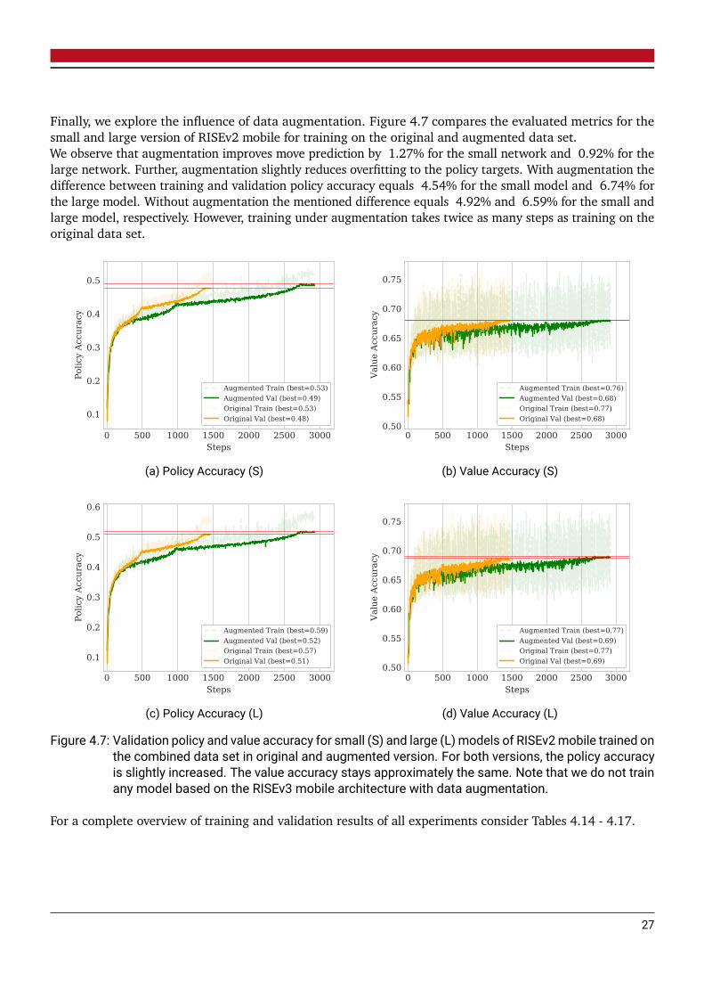
Finally, we explore the influence of data augmentation. Figure 4.7 compares the evaluated metrics for the
small and large version of RISEv2 mobile for training on the original and augmented data set.
We observe that augmentation improves move prediction by 1.27% for the small network and 0.92% for the
large network. Further, augmentation slightly reduces overfitting to the policy targets. With augmentation the
difference between training and validation policy accuracy equals 4.54% for the small model and 6.74% for
the large model. Without augmentation the mentioned difference equals 4.92% and 6.59% for the small and
large model, respectively. However, training under augmentation takes twice as many steps as training on the
original data set.
0 500 1000 1500 2000 2500 3000Steps
0.1
0.2
0.3
0.4
0.5
Polic
y Ac
cura
cy
Augmented Train (best=0.53)Augmented Val (best=0.49)Original Train (best=0.53)Original Val (best=0.48)
(a) Policy Accuracy (S)
0 500 1000 1500 2000 2500 3000Steps
0.50
0.55
0.60
0.65
0.70
0.75
Valu
e Ac
cura
cyAugmented Train (best=0.76)Augmented Val (best=0.68)Original Train (best=0.77)Original Val (best=0.68)
(b) Value Accuracy (S)
0 500 1000 1500 2000 2500 3000Steps
0.1
0.2
0.3
0.4
0.5
0.6
Polic
y Ac
cura
cy
Augmented Train (best=0.59)Augmented Val (best=0.52)Original Train (best=0.57)Original Val (best=0.51)
(c) Policy Accuracy (L)
0 500 1000 1500 2000 2500 3000Steps
0.50
0.55
0.60
0.65
0.70
0.75
Valu
e Ac
cura
cy
Augmented Train (best=0.77)Augmented Val (best=0.69)Original Train (best=0.77)Original Val (best=0.69)
(d) Value Accuracy (L)
Figure 4.7: Validation policy and value accuracy for small (S) and large (L) models of RISEv2mobile trained onthe combined data set in original and augmented version. For both versions, the policy accuracyis slightly increased. The value accuracy stays approximately the same. Note that we do not trainany model based on the RISEv3 mobile architecture with data augmentation.
For a complete overview of training and validation results of all experiments consider Tables 4.14 - 4.17.
27

Property Professional Amateur combined
Number of Games 69871 69915 139786
Number of Distinct Events 1304 1 1305
Number of Players 8440 3543 11983
Avg. Number of Moves 80 78 79
Max. Number of Moves 941 360 941
Min. Number of Moves 2 20 2
Max. Elo 2711 2629 2711
Min. Elo 2147 1515 1515
Avg. Elo 2474 1630 2052
Avg. Elo Red 2475 1630 2053
Avg. Elo Black 2473 1630 2052
Wins Red 37.07% 50.85% 43.96%
Wins Black 27.48% 46.18% 36.84%
Draws 35.45% 2.97% 19.20%
Table 4.1: Comparison of data sets of professional games and amateur games.
28

Model
RISEv2 mobilePolicy Acc Policy Loss Value Acc Value Loss Combined Loss
Pro Policy Plane (S) 0.4386 1.8694 0.7231 0.5069 1.8558
Pro One-hot (S) 0.4786 1.6810 0.7342 0.4893 1.6691
Amateur Policy Plane (S) 0.4394 1.8616 0.6303 0.8242 1.8512
Amateur One-hot (S) 0.4763 1.6938 0.6344 0.8181 1.6851
Comb Policy Plane (S) 0.4763 1.6809 0.6800 0.6676 1.6708
Comb One-hot (S) 0.5020 1.5616 0.6859 0.6599 1.5526
Comb Policy Plane (L) 0.5089 1.5288 0.6865 0.6588 1.5201
Comb One-hot (L) 0.5211 1.4753 0.6920 0.6520 1.4671
Augment Policy Plane (S) 0.4890 1.6236 0.6800 0.6674 1.6141
Augment Policy Plane (L) 0.5181 1.4938 0.6895 0.6569 1.4854
Table 4.14: Metrics on validation set for all models based on RISEv2 mobile. (S) and (L) refer to small andlarge versions of the network, respectively. Bold values mark the best performance of all models.
29

Model
RISEv2 mobilePolicy Acc Policy Loss Value Acc Value Loss Combined Loss
Pro Policy Plane (S) 0.5008 1.6646 0.7582 0.4065 1.6537
Pro One-hot (S) 0.5897 1.3036 0.7644 0.3959 1.2955
Amateur Policy Plane (S) 0.5005 1.6312 0.6629 0.7867 1.6230
Amateur One-hot (S) 0.6058 1.2607 0.6679 0.7770 1.2560
Comb Policy Plane (S) 0.5255 1.5014 0.7679 0.3995 1.4912
Comb One-hot (S) 0.5962 1.2621 0.7711 0.3985 1.2545
Comb Policy Plane (L) 0.5748 1.2955 0.7674 0.3915 1.2871
Comb One-hot (L) 0.6303 1.1198 0.7986 0.3704 1.1133
Augment Policy Plane (S) 0.5344 1.4744 0.7626 0.3985 1.4672
Augment Policy Plane (L) 0.5855 1.2392 0.7665 0.3922 1.2319
Table 4.15: Metrics on training set for all models based on RISEv2 mobile. (S) and (L) refer to small and largeversions of the network, respectively. Bold values mark the best performance of all models.
Model
RISEv3 mobilePolicy Acc Policy Loss Value Acc Value Loss Combined Loss
Comb Policy Plane (S) 0.4901 1.6114 0.6804 0.6668 1.6019
Comb Policy Plane (L) 0.5090 1.5248 0.6832 0.6624 1.5162
Table 4.16: Metrics on validation set for all models based on RISEv3 mobile. (S) and (L) refer to the small andlarge version of the network, respectively. Bold values mark the best performance of all models.
Model
RISEv3 mobilePolicy Acc Policy Loss Value Acc Value Loss Combined Loss
Comb Policy Plane (S) 0.5427 1.4431 0.7820 0.3892 1.4333
Comb Policy Plane (L) 0.5721 1.2926 0.7607 0.4071 1.2843
Table 4.17: Metrics on training set for all models based on RISEv3 mobile. (S) and (L) refer to the small andlarge version of the network, respectively. Bold values mark the best performance of all models.
30

5 Empirical Evaluation
5.1 Hardware
On any system we carry out our experiments, the underlying hardware will determine the final performance.
In general, more powerful hardware will allow an engine to perform more evaluations per time step. Especially
in our setting where we limit the maximum time of a single game and combine a neural network with MCTS,
hardware represents a critical aspect.
We compare the playing strengths of models with significant difference in complexity. More complex models
potentially reach higher prediction accuracies, but their higher inference time reduces the achievable NPS. On
the other hand, if the prediction accuracy of a less complex model is sufficiently high, it can outperform a
better predicting and more complex model as the high number of NPS might lead to better move selection. As
a consequence, a small and a large model trained on the same settings and data set can perform equally well
if they hit a sweet spot where the one’s high NPS and the other’s prediction accuracies balance each other out.
In that regard, we define the following hardware used for all our experiments:
CPU: Intel® Core™ i7-6700 CPU @ 3.40GHzx4
GPU (Training & Inference): GeForce® GTX 1070 (8GB)
GPU (Training): GeForce® GTX 1080 Ti (11GB)
Based on this hardware, we measure the NPS for all our networks on a 10 second long search at the starting
position. Figure 5.1 shows that small (S) networks reach significantly higher NPS than their large (L)
counterparts.
31

RISE
v2 O
ne-h
ot (S
)RI
SEv2
One
-hot
(L)
RISE
v2 P
olic
y Pl
ane
(S)
RISE
v2 P
olic
y Pl
ane
(L)
RISE
v3 P
olic
y Pl
ane
(S)
RISE
v3 P
olic
y Pl
ane
(L)0
2000
4000
6000
8000
NPS
Figure 5.1: NPS measured on 10 seconds search at starting position for all networks.
5.2 Tournaments
In this chapter we inspect the final playing strength of our models. We combine the trained networks with
MCTS and let them compete in tournaments.
Note that the underlying hardware for all tournaments is defined in Section 5.1. The results might differ if
performed on different hardware.
Also consider Section 7.1 for a discussion of the engine specific settings. We use the same settings for all
tournaments, as different settings might lead to different results.
Each tournament is performed in a Round Robin fashion. Each game starts at a random position at maximum
100 plys deep. Per encounter, two models compete in two games while they share the same opening for each
game. We set the Time Control to one minute, with an potential increment of 0.25 seconds.
In our first tournament we primarily inspect the influence of the data set on a models’ playing strength.
Additionally, we get a first idea about the consequence of our policy representation. Table 5.1 shows the
outcome of the tournament. All models are based on the small variant of the RISEv2 mobile architecture
(Table 4.4).
We observe that training on the combined data set yields the best performance. Also, with exception to models
trained on professional games, using a policy plane representation further improves the playing strength of a
model. This is contrary to our supervised learning results (Table 4.14). In supervised learning we observe that
models based on a one-hot encoded policy representation outperform those based on a plane representation on
every metric. This indicates that a plane policy representation helps the model to generalize: When confronted
with unforeseen moves, the model is able to find better responses.
This effect is canceled by training on data of exclusively professional players. As we can observe in Figure
4.5a, training solely on professional games leads to strong overfitting independent of our choice of policy
representation. As a consequence, these models cannot find appropriate responses to moves not occurring in
the data set. Figure 5.2 summarizes our observations by comparing the relative elo of all models.
32

Com
b Po
licy
Plan
e (S
)Co
mb
One
-hot
(S)
Amat
eur
Polic
y Pl
ane
(S)
Amat
eur
One
-hot
(S)
Pro
One
-hot
(S)
Pro
Polic
y Pl
ane
(S)
0
200
400
Rel
ativ
e E
lo
Figure 5.2: Elo comparison for small models of RISEv2 mobile architecture.
Table 5.2 shows the results of multiple one-on-one tournaments between RISEv2 mobile based models trained
on the combined and augmented data set.
First, we observe that for large models (Table 4.5) (Comb One-hot (L) vs. Comb Policy Plane (L)) using the plane
policy representation still yields the best performance. The additional parameters as a result of the one-hot
vector encoding (Table 4.13) lead to slightly lower NPS (Figure 5.1). Combined with the lower generalization
ability of this architecture, its playing strength is inferior.
Next, the large model outperforms the small model (Comb Policy Plane (S) vs. Comb Policy Plane (L)). This
is despite the fact that the large model only reaches approximately half the NPS of the smaller one. On the
validation set the policy accuracies (50.89% vs. 47.63%) and the value accuracies (68.65% vs. 68.00%) are
both higher for the large model. As a consequence, the large model needs far less evaluations to select better
moves than its small counterpart.
We make a third observation which is that data set augmentation slightly harms the playing strength of a
model. This is true for the small and the large network and contrary to our expectations. When evaluating
these models in the context of supervised learning (Figure 4.7), we actually notice a small improvement on all
metrics. In this regard we do not find any meaningful reason for this outcome.
33

Rank Model Games Score Draws
1 Comb Policy Plane (S) 100 82.5% 27.0%
2 Comb One-hot (S) 100 67.0% 20.0%
3 Amateur Policy Plane (S) 100 53.0% 28.0%
4 Amateur One-hot (S) 100 48.5% 19.0%
5 Pro One-hot (S) 100 27.5% 23.0%
6 Pro Policy Plane (S) 100 21.5% 21.0%
Table 5.1: Tournament of small RISEv2mobile basedmodels. We train a model for each policy representationand data set (including the combined data set).
Tournament Games Result Draw Ratio Elo difference
Comb One-hot (L)
vs.
Comb Policy Plane (L)
100 0 - 92 - 8 8.0% −552.1 +/− 143.7
Comb Policy Plane (S)
vs.
Augment Policy Plane (S)
200 55 - 52 - 93 46.5% +5.2 +/− 35.3
Comb Policy Plane (L)
vs.
Augment Policy Plane (L)
200 47 - 39 - 114 57.0% +13.9 +/− 31.6
Comb Policy Plane (S)
vs.
Comb Policy Plane (L)
200 3 - 127 - 70 35.0% −251.9 +/− 40.6
Table 5.2: Results of tournaments for small (S) and large (L) models based on the RISEv2 mobile architecture.Result reads Wins - Losses - Draws with respect to the first model mentioned. The Elo differenceis given relative to the second model mentioned.
At this point we observed that our strongest models are trained on the combined data set while using a plane
policy representation. Furthermore, the large version of RISEv2 mobile performs better than the small version.
In our final experiment we try to improve our best approaches by upgrading the models’ architectures to
RISEv3 mobile.
Table 5.3 shows that upgrading the small model to RISEv3 mobile significantly increases the performance
34

(RISEv2 mobile (S) vs. RISEv3 mobile (S)). We observe a relative elo difference of -65.0 +/- 35.4 for the RISEv2
mobile architecture relative to the RISEv3 mobile architecture.
On the contrary, the tournament of our large models (RISEv2 mobile (L) vs RISEv3 mobile (L)) indicates only a
slight improvement. This is unexpected, as we use SE blocks in all 13 residual blocks for the RISEv3 mobile
architecture, instead of only in the last 5 residual blocks as for the RISEv2 mobile architecture (Section 4.6).
It is questionable whether the higher computational effort is worth its cost.
Finally, we observe that even though we significantly improved our small models’ performance compared to
only a small improvement for our large model, the large model still outperforms the small one (RISEv3 mobile
(S) vs. RISEv3 movile (L)). However, the small model now reaches a draw ratio of 42% instead of only 35% in
the case of the RISEv2 mobile architecture. This reflects the scope of our observed improvements for each
model.
We conclude that of all our approaches the large variant of the RISEv3 mobile architecture performs best. In
addition, our models all benefit from the diversity of the combined data set and the plane policy representation.
35

Tournament Games Result Draw Ratio Elo difference
RISEv2 mobile (S)
vs.
RISEv3 mobile (S)
200 35 - 72 - 93 46.5% −65.0 +/− 35.4
RISEv2 mobile (L)
vs.
RISEv3 mobile (L)
200 44 - 48 - 108 54.0% −6.9 +/− 32.7
RISEv3 mobile (S)
vs.
RISEv3 mobile (L)
100 3 - 55 - 42 42.0% −200.2 +/− 52.6
Table 5.3: Results of tournaments between RISEv2 mobile and RISEv3 mobile. All models are trained on thecombined data set using a plane policy representation. Result reads Wins - Losses - Draws withrespect to the first model mentioned. The Elo difference is given relative to the second modelmentioned.
5.3 General Observations
We test the influence of the move distribution in our data set used for training on the prediction of the first
move by our large RISEv3 mobile based network. Also, we see how the win-draw-loss ratio of the data set
determines the value prediction in the first state. We then combine our network with MCTS and see whether
a search conducted over 10 seconds yields any changes.
Figure 5.3 shows the five most common moves in the single data sets of amateur and professional players. We
observe, that move h2e2 is by far the most played opening move in both data sets. Further, in both data sets
moves h2d2 and c3c4 are part of the five most common first moves.
As a consequence, these relations are reflected in the combined data set (Figure 5.4b). Additionally, Figure
5.3a shows a visualization of these moves.
If we take a look at Table 4.1, we observe that in the combined data set the red player wins most of the time
(43.96%). As the first player to move in chinese chess is the red player, we expect the network to slightly
prefer predicting a win at the starting position.
Our model predicts move h2e2 with 42.19% certainty for the starting position of any game. Because this move
is highly overrepresented in the data set we used to train it, this is what we expect. We can further observe
that the models’ certainty is higher than the relative occurrence of move h2e2 in all opening moves (38.05%).
Also, as we expected, the models’ value prediction is slightly biased towards a win for the red player. Its value
output is 0.08 and we use a value of 1 to decode a win for the current player.
If we now combine our model with MCTS and perform a 10 second search at the starting position we get a
different result. Table 5.4 shows, that instead of move h2e2 now move c3c4 is evaluated as most promising.
We can further see that move h2e2 has the highest policy evaluation, but as c3c4 is visited much more often,
the search algorithm starts to prefer move c3c4 based on its higher Q-value.
36

Move Visits Policy Q-values CP
c3c4 23375 0.1391085 0.1291571 75
h2e2 2688 0.2297229 0.0770245 43
b2e2 1541 0.0680645 0.1034426 59
g0e2 1215 0.1014676 0.0779215 44
g3g4 1069 0.0711157 0.0887958 51
Table 5.4: MCTS evaluation based on the large version of RISEv3 mobile. Search was performed over 10seconds at the starting position.
h2e2 b2e2 g3g4 c3c4 h2d2Move
0
5
10
15
20
25
30
Percen
tage
(a) Amateur
h2e2 c3c4 g0e2 b0c2 h2d2Move
0
10
20
30
40
Percen
tage
(b) Professional
Figure 5.3: Top 5 most common moves in the data sets of (a) amateur players and (b) professional players.
5.4 Relative Strength
In this section we put our strongest approach to the test against version 11.2 of Fairy-Stockfish1. Fairy-Stockfish
is one of the strongest publicly availabe chess variant engines that support chinese chess. In chinese chess,
Fairy-Stockfish reaches a playing strength at least on master level2.
The playing strength of Fairy-Stockfish was evaluated against reference engines. Table 5.5 shows Fairy-
Stockfishs’ Elo relative to other engines.
Our strongest model is the large version of the RISEv3 mobile architecture trained on the combined data set.
The tournament against Fairy-Stockfish is performed under the same settings as our experiments (Section
1https://github.com/ianfab/Fairy-Stockfish, accessed April 19, 20212https://github.com/ianfab/Fairy-Stockfish/wiki/Playing-strength, accessed April 19, 2021
37

(a) Visualization of the 5 most common first moves.
h2e2 c3c4 g3g4 g0e2 b2e2Move
0
5
10
15
20
25
30
35
Percen
tage
(b) Percentage of the 5 most common first moves.
Figure 5.4: (a) Visualizes the 5 most common moves in the combined data set. From left to right, top tobottom: c3c4, g3g4, b2e2, h2e2, g0e2. (b) Shows their distribution over all possible first moves.h2e2 is by far the most common.
5.2). We also use the same hardware as described in Section 5.1.
The result of 100 games between the large variant of RISEv3 mobile and Fairy-Stockfish is shown in Table
5.6. Fairy-Stockfish reaches a relative elo of +322.7 +/- 77.0. Compared to the reference engines mentioned
before, our model reaches a performance comparable to that of Sjaak II. Even under consideration of an
uncertainty of +/- 77.0 Elo points, our model reaches a higher relative Elo than MaxQi.
38

Reference Engine Relative Elo
Cyclone 0.553 +100
Elephant Eye 3.314 +100
Sjaak II5 +300
MaxQi6 >+500
Table 5.5: Reference engines and Fairy-Stockfishs’ Elo relative to them. Of all tested engines, Fairy-Stockfishreaches the highest playing strength.
Table 5.6: Tournament results of the large variant RISEv3 mobile and Fairy-Stockfish on 100 games. Ourmodel was trained on the combined data set and uses a plane policy representation.
Tournament Games Result Draw Ratio Elo difference
Fairy-Stockfish
vs.
RISEv3 mobile (L)
100 76 - 3 - 21 21.0% +322.7 +/− 77.0
39

6 Conclusion
6.1 Summary
In this work we evaluated the performance of two different architectures, both optimized for integration into
MCTS. We trained our networks in a supervised learning setting and compared their playing strength based
on multiple tournaments.
Our evaluations showed the significance not only of the size, but also of the diversity of a data set used to train
a neural network in the domain of chinese chess. We demonstrated that even data sets of professional players
can result in models with weak playing strength, if the data set is not sufficiently large. Also we compared two
representations for our policy targets. By encoding information about the spatial correlation of moves into our
policy representation, the network is able to generalize better. This is despite the fact that a more complex
model that uses a one-hot vector encoding outperforms the plane policy representation on all supervised
learning metrics. In a last experiment we showed the influence of MCTS on move selection. Although in our
data set a single move dominates being played in the starting position, MCTS expands the evaluation to a
different move.
Finally, we tested our strongest approach against Fairy-Stockfish. Even though Fairy-Stockfish outperforms
our model, it is able to reach results comparable to other engines that were evaluated against Fairy-Stockfish.
6.2 Future work
Future work should either focus on a larger data set or rely on self-play. The definitive bottleneck of our
approach is the restricted quantity of available data. As a result, our models struggle to generalize. When
training on self-play we can bypass this problem. Projects as AlphaZero [10] show that we are able to build
generalized approaches that reach superhuman performance through self-play. However, self-play drastically
increases the hardware requirements.
A different approach to better performance is further tweaking our network architectures. Especially in the
case of the small variants of RISEv2 mobile and RISEv3 mobile we have seen that minor adjustments can lead
to significant performance inceases.
40

Acknowledgements The author thanks Johannes Czech for his support and patience throughout this work.
Further, the author thanks the Artificial Intelligence and Machine Learning Lab of TU Darmstadt for the
possibility to work on an exciting project and the access to a GPU-Server that was of significant help. The
author also thanks the developers of cutechess for a convenient way to conduct tournaments between engines,
especially gaintpd for implementing the support of chinese chess. Finally, the author thanks all developers of
Stockfish, Multi-Variant-Stockfish and Fairy-Stockfish for providing these exciting open source projects.
41

Bibliography
[1] Johannes Czech et al. ”Learning to play the Chess Variant Crazyhouse above World Champion Level with
Deep Neural Networks and Human Data”. In: arXiv preprint arXiv:1908.06660 (2019).
[2] Johannes Czech. ”Deep Reinforcement Learning for Crazyhouse”. https://www.ml.informatik.tu-
darmstadt.de/papers/czech2019deep.pdf. (Accessed April 19, 2021).
[3] Johannes Czech, Patrick Korus, Kristian Kersting. ”Monte-Carlo Graph Search for AlphaZero”. In:
arXiv:2012.11045 (2020).
[4] Stefan-Meyer Kahlen. UCI Protocol. http://wbec-ridderkerk.nl/html/UCIProtocol.html. (Accessed April
19, 2021).
[5] Leslie N Smith and Nicholay Topin. ”Super-convergence: Very fast training of neural networks using large
learning rates”. In: Artificial Intelligence and Machine Learning for Multi-Domain Operations Applications.
Vol. 11006. International Society for Optics and Photonics. 2019, p. 1100612.
[6] Xavier Glorot and Yoshua Bengio. ”Understanding the difficulty of training deep feedforward neural
networks”. In: Proceedings of the thirteenth international conference on artificial intelligence and statistics.
2010, pp. 249–256.
[7] Aleksandar Botev, Guy Lever, David Barber. ”Nesterov’s accelerated gradient and momentum as approxima-
tions toregularised update descent”. In: 2017 International Joint Conference on Neural Networks (IJCNN).
IEEE. 2017, pp. 1899-1903.
[8] Silver, D., Huang, A., Maddison, C. et al. ”Mastering the game of Go with deep neural networks and tree
search”. In: Nature 529 (2016), pp. 484-489.
[9] Silver, D., Schrittwieser, J., Simonyan, K. et al. ”Mastering the game of go without human knowledge”. In:
Nature 550 (2017), pp. 354-359.
[10] David Silver, Thomas Hubert, Julian Schrittwieser, Ioannis Antonoglou, Matthew Lai, Arthur Guez, Marc
Lanctot, Laurent Sifre, Dharshan Kumaran, Thore Graepel, Timothy Lillicrap, Karen Simonyan, Demis
Hassabis. ”Mastering Chess and Shogi by Self-Play with a General Reinforcement Learning Algorithm”.
In: arXiv:1712.01815 (2017).
[11] Andrew G. Howard, Menglong Zhu, Bo Chen, Dmitry Kalenichenko, Weijun Wang, Tobias Weyand,
Marco Andreetto, Hartwig Adam. ”MobileNets: Efficient Convolutional Neural Networks for Mobile Vision
Applications”. In: arXiv:1704.04861 (2017).
[12] Mark Sandler, Andrew Howard, Menglong Zhu, Andrey Zhmoginov, Liang-Chieh Chen. ”MobileNetV2:
Inverted Residuals and Linear Bottlenecks”. In: arXiv:1801.04381 (2018).
42

[13] Andrew Howard, Mark Sandler, Grace Chu, Liang-Chieh Chen, Bo Chen, Mingxing Tan, Weijun Wang,
Yukun Zhu, Ruoming Pang, Vijay Vasudevan, Quoc V. Le, Hartwig Adam. ”Searching for MobileNetV3”.
In: arXiv:1905.02244 (2019).
[14] Kaiming He, Xiangyu Zhang, Shaoqing Ren, Jian Sun. ”Deep Residual Learning for Image Recognition”.
In: arXiv:1512.03385 (2015).
[15] Jie Hu, Li Shen, Samuel Albanie, Gang Sun, Enhua Wu. ”Squeeze-and-Excitation Networks”. In:
arXiv:1709.01507 (2017).
[16] Yann LeCun, Yoshua Bengio. ”Convolutional Networks for Images, Speech, and Time-Series”. In: The
Handbook of Brain Theory and Neural Networks (1995).
[17] Dongyoon Han, Jiwhan Kim, Junmo Kim. ”Deep Pyramidal Residual Networks”. In: arXiv:1610.02915
(2016).
[18] Sanghyun Woo, Jongchan Park, Joon-Young Lee, In So Kweon. ”CBAM: Convolutional Block Attention
Module”. In: arXiv:1807.06521 (2018).
43

7 Appendix
7.1 Engine Settings
Parameter Value
Allow_Early_Stopping true
Batch_Size 16
Centi_CPuct_Init 250
Centi_Dirichlet_Epsilon 0
Centi_Dirichlet_Alpha 20
Centi_Node_Temperature 170
Centi_Q_Value_Weight 0
Centi_Q_Thresh_Init 50
Centi_Q_Thresh_Max 90
Centi_Quantile_Clipping 25
Centi_Random_Move_Factor 0
Centi_Temperature 170
Centi_Temperature_Decay 92
Centi_U_Init_Divisor 100
Centi_Virtual_Loss 100
Context gpu
CPuct_Base 19652
Enhance_Checks false
First_Device_ID 0
Fixed_Movetime 0
Last_Device_ID 0
Max_Search_Depth 99
MCTS_Solver true
Move_Overhead 20
Nodes 0
Precision float16
Table 7.1: Engine settings (Part 1).
44

Parameter Value
Q_Thresh_Base 1965
Random_Playout false
Reuse_Tree true
Temperature_Moves 0
Use_Advantage false
Use_NPS_Time_Manager false
Use_TensorRT true
Use_Transposition_Table true
Search_Type mcts
Simulations 0
Threads 4
Use_Raw_Network false
Protocol uci
Contempt 24
Analysis Contempt Both
Clear Hash
MultiPV 1
Skill Level 20
Move Overhead 10
Slow Mover 100
nodestime 0
UCI_LimitStrength false
UCI_Elo 1350
SyzygyPath <empty>
SyzygyProbeDepth 1
Syzygy50MoveRule true
SyzygyProbeLimit 7
Table 7.2: Engine settings (Part2 ).
45