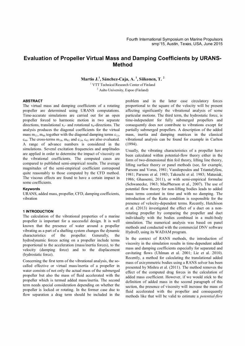
evaluation of propeller virtual mass and damping ... · evaluation of propeller virtual mass and...
TRANSCRIPT
Fourth International Symposium on Marine Propulsors smp’15, Austin, Texas, USA, June 2015
Evaluation of Propeller Virtual Mass and Damping Coefficients by URANS-
Method
Martio J.1, Sánchez-Caja, A. 1, Siikonen, T. 2
1 VTT Technical Research Center of Finland 2 Aalto University, Espoo (Finland)
ABSTRACT The virtual mass and damping coefficients of a rotating propeller are determined using URANS computations. Time-accurate simulations are carried out for an open propeller forced to harmonic motion in two separate directions, translational x1- and rotational x4-directions. The analysis produces the diagonal coefficients for the virtual mass m11, m44 together with the diagonal damping terms c11, c44. The cross-terms m14, m41 and c14, c41 are also evaluated. A range of advance numbers is considered in the simulations. Several excitation frequencies and amplitudes are applied in order to determine the impact of viscosity on the vibrational coefficients. The computed cases are compared to published semi-empirical results. The average magnitudes of the semi-empirical coefficient correspond quite reasonably to those computed by the CFD method. The viscous effects are found to have a certain impact in some coefficients. Keywords URANS, added mass, propeller, CFD, damping coefficients, vibration 1 INTRODUCTION The calculation of the vibrational properties of a marine propeller is important for a successful design. It is well known that the presence of water around a propeller vibrating as a part of a shafting system changes the dynamic characteristics of the propeller. Generally, the hydrodynamic forces acting on a propeller include terms proportional to the acceleration (mass/inertia forces), to the velocity (damping force) and to the displacement (hydrostatic force). Concerning the first term of the vibrational analysis, the so-called effective or virtual mass/inertia of a propeller in water consists of not only the actual mass of the submerged propeller but also the mass of fluid accelerated with the propeller which is termed added mass/inertia. The second term needs special consideration depending on whether the propeller is locked or rotating. In the former case due to flow separation a drag term should be included in the
problem and in the latter case circulatory forces proportional to the square of the velocity will be present affecting significantly the vibrational analysis of some particular motions. The third term, the hydrostatic force, is time-independent for fully submerged propellers and consequently does not contribute to vibrations except for partially submerged propellers. A description of the added mass, inertia and damping matrices in the classical vibrational analysis can be found for example in Carlton (1994). Usually, the vibrating characteristics of a propeller have been calculated within potential-flow theory either in the form of two-dimensional thin foil theory, lifting line theory, lifting surface theory or panel methods (see, for example, Parsons and Vorus, 1981; Vassilopoulos and Triantafyllou, 1981; Parsons et al. 1983; Takeuchi et al. 1983; Matusiak, 1986; Ghassemi, 2011), or with semi-empirical formulae (Schwanecke, 1963; MacPherson et al., 2007). The use of potential flow theory for non-lifting bodies leads to added mass terms constant in time and with no damping. The introduction of the Kutta condition is responsible for the presence of velocity-dependent terms. Recently, Hutchison et al. (2013) investigated the effect of a duct on a non-rotating propeller by comparing the propeller and duct individually with the bodies combined in a multi-body simulation. The numerical analysis was based on panel methods and conducted with the commercial DNV software HydroD, using its WADAM program. In the context of RANS methods, the introduction of viscosity in the simulation results in time-dependent added mass and damping coefficients especially for separated and cavitating flows (Uhlman et al. 2001; Lie et al. 2010). Recently, a method for calculating the translational added mass of axisymmetric bodies using a RANS solver has been presented by Mishra et al. (2011). The method removes the effect of the computed drag forces in the calculation of added mass coefficient. However, if we would stick to the definition of added mass in the second paragraph of this section, the presence of viscosity will increase the mass of fluid accelerated with the propeller and consequently methods like that will be valid to estimate a potential-flow

added mass using a viscous solver, but not a viscous added mass. Much attention has been paid in the literature to the computation of the added mass coefficients for circular cylinders in various regimes of viscous flow and oscillating wings. However, to our knowledge there is a gap concerning the computations of such coefficients by RANS methods for rotating propellers. The present paper shows computations of added mass and damping coefficients for coupled torsional-axial motion and illustrates their variation as a function of the excitation frequency and advance number of the propeller. The virtual mass and damping of a propeller are evaluated in viscous flow using URANS-method solver FINFLO (Sánchez-Caja et al., 1999; Siikonen, 2011). The coefficients are determined for a range of advance number J = [0.2,…,1.2]. The exciting frequency is varied between 0.25 and 1.6 times the blade passing frequency. A propeller working in open flow is analyzed in the computations. The study is made at model scale. 2 NUMERICAL METHOD 2.1 Governing equations The Navier-Stokes momentum equation can be written for a control volume delimited by a boundary as follows,
( )
+ ( )( )
=( )
+( )
(1)
where is the flow velocity vector, is the velocity vector on the boundaries, p is the pressure in the flow field , is the vector normal to the boundary and is the viscosity. The boundary ( ) consists of a moving boundary attached to the surfaces of an oscillating body and an external and stationary boundary which may extend to infinity. The fluid velocity vector can be separated into three components by applying the Helmholtz decomposition:
= + + (2)
where is the uniform inflow velocity at infinity upstream, is the velocity field by the perturbation potential and is the velocity component due viscous effects. The last term will be responsible for the viscous component of the added mass. On the other hand, if the propeller is moving in unidirectional motion and simulatenously in harmonic motion, the instantaneous state vector is [ , + , ]. The speed of advance can be treated as a steady velocity component with the magnitude
same as into the given direction xi, where i=1…3. The harmonic velocity term and the harmonic acceleration are defined as follows,
= sin( ) = cos( ) (3)
where is the velocity amplitude of the harmonic motion to the given direction xi, i=1…6. If the control volume is large enough, the convection term at the left side of Eq. (1) vanishes in global sense. Using the instantaneous velocity + , Eq. (1) can be made non-dimensional as follows,
+ ( + )
=( )
+( )
(4)
where is the non-dimensiolized fluid velocity and t0 a time made non-dimensional with the inverse of the propeller rotational speed n. Notice that as the term used for non-dimensionalization is time-dependent but not space-dependent, it can be transferred outside the integral. The force components of Eq. (4) can be expressed as
+ + = ( ) (5)
The first term is the acceleration-related added mass term, the second term is the damping term associated to the harmonic velocity component and the third term is force component generated by propeller’s average thrust. Eq. (4) can be made non-dimensional in space using the propeller diameter D and approximated by the following linear semi-empirical fitting for the translational oscillations in direction x1,
+ + = ( ) (6)
The corresponding formulation applied to the rotational oscillations in direction x4 is + + = ( ) (7)
The thrust and torque coefficients, the diagonal elements of the virtual mass matrix and the diagonal damping terms are defined as follows, = =
= =
= =
(8)
The cross-terms related rotational motion are evaluated as follows,

+ + = ( ) (9)
where, = =
= = (10)
The coefficients are expressed in terms of the frequency ratio fe/f (fe is the excitation frequency and f the blade passing frequency) and a set of selected dimensionless parameters describing the flow conditions. For example, in the direction x1 the dimensionless parameters are as follows, = =
= = (11)
where n is the propeller revolutions. The advance number J is related to the average loading on the propeller, whereas the Keulegan-Carpenter number KC, the Reynolds number Re and the Stokes parameter are associated to the harmonic flow components. The physical background of the harmonic key figures is similar to those used to categorize the flow patterns of an oscillating cylinder. In this paper, the evaluated force coefficients are parametrized by J and fe/f. 2.2 URANS solver FINFLO The flow simulation in FINFLO is based on the solution of the RANS equations by the pressure correction method. The spatial discretization is carried out by a finite volume method. The solution is based on approximately factorized time-integration with local time stepping. The second and third order upwind biased scheme is used for the discretization of the convection terms. Second order central-difference scheme is utilized for the discretization of the diffusion terms. The code uses an incompressible flux-difference splitting. A multigrid method is applied for the acceleration of convergence. Solutions in coarse grid levels are used as starting point for the calculation in order to accelerate convergence. A detailed description of the numerical method including discretization of the governing equations, solution algorithm, boundary conditions, etc. can be found in Sánchez-Caja et al. (1999) and Siikonen (2011). Several turbulence models are implemented in FINFLO. In these calculations Chien’s low Reynolds number k- turbulence model is used. Time-accurate calculations are started by using the quasi-steady solution as the initial guess. In the time-accurate calculations part of the grid is rotating at the propeller rotational speed and part of the grid is stationary. The sliding mesh technique is used to treat the interface between the rotating and the stationary part of the grid. The solution is interpolated using the solution in the neighboring blocks.
FINFLO computational approach includes also the possibility to use the overlapping grid technique (Chimera). Table I. Geometrical data of the P1374 model propeller.
Propeller diameter 250.0 mm Number of blades Z 4 Pitch/Diameter at r/R=0.7 1.1
Hub diameter 60.0 mm Expanded area ratio 0.602 Expanded skew angle 23 deg
Figure 1: RANS grid on the blades of propeller P1374. 3 STUDY CASES 3.1 The P1374 propeller The P1374 propeller and related experimental data used in this research were provided by MARINTEK (Koushan, 2006). The main parameters of the propeller are shown in Table I. A perspective view of the propeller geometry with the grid on the blades is presented in Fig. 1. As it can be seen from the figure, the grid is very dense on the blades. It consists of 27 blocks with a total of 5.3 million cells for a blade passage.
3.2 Boundary conditions for harmonic oscillations The computational grid covers a single-blade passage so that cyclic boundary conditions can be applied on the appropriate boundaries. On the blade surface, a non-slip boundary condition was used on the rotating blades (ROT), whereas on the nozzle surface a stationary non-slip boundary condition was utilized. In the external boundaries inlet and outlet boundary conditions on velocity and pressure, respectively were applied. The ROT-condition

was modified to enforce oscillating motions in the x1 and x4-directions. The additional harmonic component on the grid and solid surfaces (ALE method) was: = sin( ) (12)
which resulted in an instantaneous acceleration = cos( ) (13)
with equal to for the term and for the term.
The parameters used in rotational oscillations are presented in Table II. The case with excitation frequency fe=9.0 Hz and amplitude x4a=5.0 deg was evaluated for three advance numbers J=0.40, 0.60 and 0.80. The blade passing frequency was f=36.0 Hz in all cases. Table II. Parameters for the rotational oscillations.
Case Excitation frequency
fe [1/s]
Angle amplitude
[deg]
Velocity amplitude
[deg/s]
Advance number
1.1 9.0 5.0 282.7 0.40
1.2 9.0 5.0 282.7 0.60
1.3 9.0 1.0 56.5 0.80
1.4 22.5 1.0 141.4 0.80
1.5 40.5 1.0 254.5 0.80
1.6 9.0 5.0 282.7 0.80
1.7 22.5 5.0 706.9 0.80
The corresponding parameters applied in the translational oscillations are shown in Table III. The computations of the ducted propeller were carried out for two rotational motions and for two translational harmonic motions. The related parameters were x4a=1.0 deg and 5.0 deg using fe=22.5 Hz and x1a=6.37 m/s with fe=22.5 Hz and 23.9 m/s using fe=40.5 Hz applied to the rotational motion x4 and the translational motion x1, respectively. The computations of combined translational and rotational motions were evaluated also in order to detect if the superposition principle holds for the simulated cases. The oscillations in direction x4 corresponded the case 1.4 and in direction x1 the case 2.9. 4 RESULTS 4.1 Open water characteristics The open water performance was computed for the open propeller. Figure 2 and Table IV show the performance coefficients evaluated by FINFLO compared to the
experimental values. The characteristics of the ducted propeller were evaluated only for the advance number J=0.8.
Table III. Parameters for the translational oscillations.
Case
Excitation frequency
fe
[1/s]
Displace-ment
amplitude
[m]
Velocity amplitude
[m/s]
Accelera-tion
amplitude
[m/s ]
Advance number
J
2.1 22.5 0.00113 0.0601 8.5 0.2
2.2 49.5 0.00051 0.0283 8.8 0.2
2.3 31.5 0.00080 0.0641 12.68 0.2
2.4 31.5 0.00080 0.0913 18.07 0.2
2.5 57.9 0.00044 0.0568 20.67 0.2
2.6 40.5 0.00063 0.0938 23.88 0.2
2.7 40.5 0.00063 0.1037 26.4 0.2
2.8 22.5 0.00113 0.0451 6.37 0.8
2.9 22.5 0.00113 0.0601 8.5 0.8
2.10 49.5 0.00051 0.0283 8.8 0.8
2.11 31.5 0.00080 0.0913 18.07 0.8
2.12 57.9 0.00044 0.0568 20.67 0.8
2.13 40.5 0.00063 0.0938 23.88 0.8
2.14 40.5 0.00063 0.1037 26.4 0.8
2.15 40.5 0.00063 0.1241 31.57 0.8
2.16 49.5 0.00051 0.0283 8.8 1.2
2.17 31.5 0.00080 0.0913 18.07 1.2
2.18 49.5 0.00051 0.0816 25.37 1.2
2.19 40.5 0.00063 0.1241 31.57 1.2
4.2 Added inertia and damping
Rotational motion Cases 1.3 and 1.7 are presented in Figure 3. The computed forces of case 1.3 include some non-linear elements, whereas case 1.7 features apparently almost purely linear oscillations. Case 1.7 can be considered as an extreme case, as the thrust and the torque both are reversed during the simulations. The thrust coefficient KT is presented as a function of x4a in Figure 4. The amplitude does not seem to have almost any impact on the average thrust (less than 1.5%) and torque (about 2%). Only the extreme case 1.7 produces larger magnitude of KT, KQ coefficients compared to the non-oscillating case (near 8%).
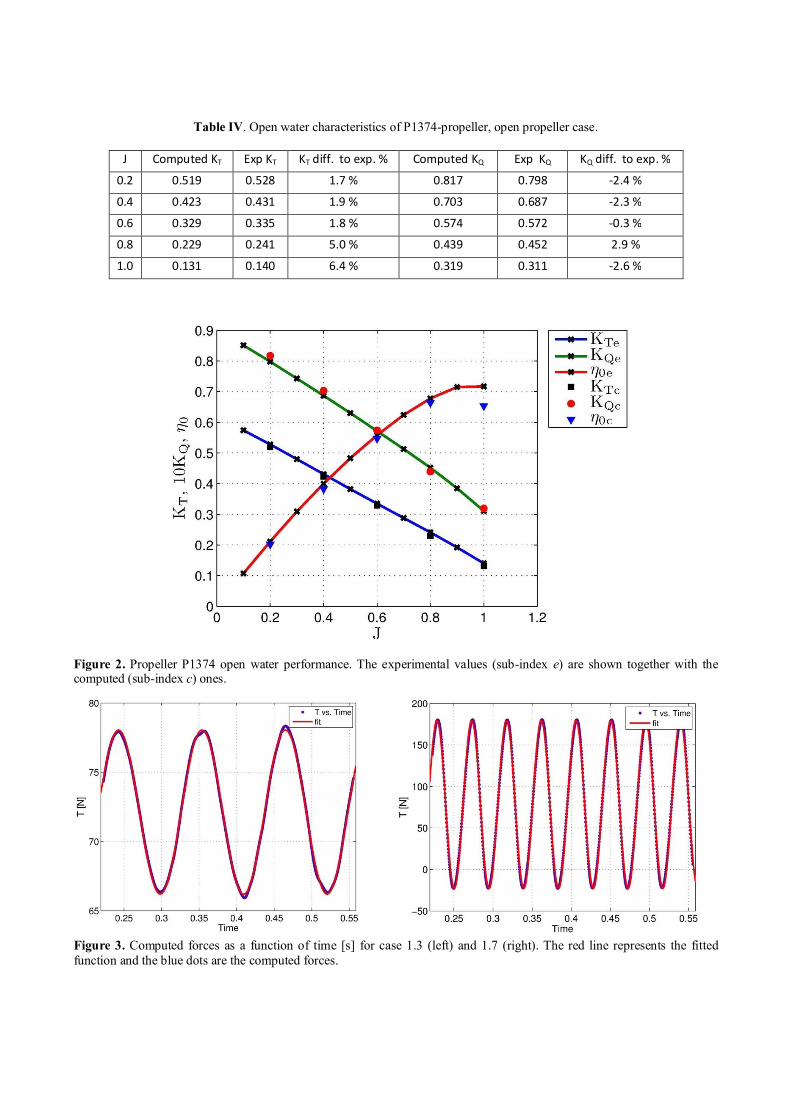
Table IV. Open water characteristics of P1374-propeller, open propeller case.
Figure 2. Propeller P1374 open water performance. The experimental values (sub-index e) are shown together with the computed (sub-index c) ones.
Figure 3. Computed forces as a function of time [s] for case 1.3 (left) and 1.7 (right). The red line represents the fitted function and the blue dots are the computed forces.
J Computed KT Exp KT KT diff. to exp. % Computed KQ Exp KQ KQ diff. to exp. %
0.2 0.519 0.528 1.7 % 0.817 0.798 -2.4 %
0.4 0.423 0.431 1.9 % 0.703 0.687 -2.3 %
0.6 0.329 0.335 1.8 % 0.574 0.572 -0.3 %
0.8 0.229 0.241 5.0 % 0.439 0.452 2.9 %
1.0 0.131 0.140 6.4 % 0.319 0.311 -2.6 %

Figure 4: Thrust coefficient KT as a function of amplitude
x4a. The advance numbers are in different colors.
Figure 5. Computed force as a function of time for case 1.7. Total thrust force T, pressure component Tp and the viscous component Tv.
Figure 6a: Added mass coefficient m44 as a function of the ratio of the excitation frequency to blade passing frequency and of the advance number J. The blue line corresponds to the semi-empirical method by [Schwanecke].
Figure 6b: Damping coefficient c44 as a function of the ratio of the excitation frequency to blade passing frequency and of the advance number J. The blue line corresponds to the semi-empirical method by [Schwanecke].
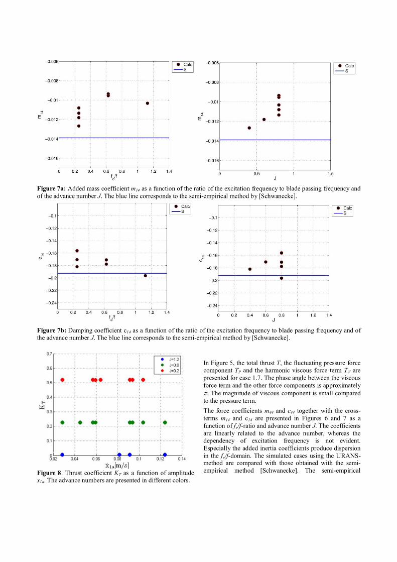
Figure 7a: Added mass coefficient m14 as a function of the ratio of the excitation frequency to blade passing frequency and of the advance number J. The blue line corresponds to the semi-empirical method by [Schwanecke].
Figure 7b: Damping coefficient c14 as a function of the ratio of the excitation frequency to blade passing frequency and of the advance number J. The blue line corresponds to the semi-empirical method by [Schwanecke].
Figure 8. Thrust coefficient KT as a function of amplitude x1a. The advance numbers are presented in different colors.
In Figure 5, the total thrust T, the fluctuating pressure force component TP and the harmonic viscous force term TV are presented for case 1.7. The phase angle between the viscous force term and the other force components is approximately
. The magnitude of viscous component is small compared to the pressure term. The force coefficients m44 and c44 together with the cross-terms m14 and c14 are presented in Figures 6 and 7 as a function of fe/f-ratio and advance number J. The coefficients are linearly related to the advance number, whereas the dependency of excitation frequency is not evident. Especially the added inertia coefficients produce dispersion in the fe/f-domain. The simulated cases using the URANS-method are compared with those obtained with the semi-empirical method [Schwanecke]. The semi-empirical

method does not yield good correlation for the rotational motion related coefficients as seen in Figures 6 and 7a. In the figures, different advance numbers for the same frequency are located in the same vertical line and viceversa (different frequencies for the same advance number). Finally, selected local flow quantities are displayed in Figures A1-A3 in the Appendix. The pressure field and u-velocity distribution are shown on the blades and at cut y=0, respectively. The pressure coefficient is defined as follows,
= 0.5 ( ) (14)
The analysis is conducted at some representative values of t (45, 90 and 180 deg) for the cases 1.3 and 1.6. The larger
amplitude of the case 1.6 produces a distorted wake profile shown in Figure A3. The effect of oscillations is also clearly seen on the pressure field on the blades, Figures A1-A2. The pressure impact due the harmonic motion is distributed quite uniformly on the blades.
The wake of the case 1.3 shown in Figure A3 is also influenced by the oscillations, but the u-velocity field remains still quite straight. Translational motion The time histories of the total thrust force T and of the viscous and pressure components are similar to the rotational motion case. They include some non-linearities in the viscous term, being again the magnitude of viscous component rather small compared to the pressure component. They are not presented here. The KT coefficient is shown as a function of the excitation amplitude in Figure 8. The oscillations produce only minor impacts to the average thrust force, of the order of 1% or less for cases 2.1-2.15. As the advance number is increased, the oscillations seem to reduce the KT as compared to the non-oscillating cases.
Figure 9. Added mass m11 and damping coefficient c11 as a function of the ratio of the excitation frequency to blade passing frequency and of the advance number J. The blue line corresponds to the semi-empirical method by [Schwanecke].

Figure 10. Added mass coefficients m41 and damping coefficient c41 as a function of the ratio of the excitation frequency to blade passing frequency and of the advance number J. The blue line corresponds to the semi-empirical method by [Schwanecke].
The harmonic coefficients m11, c11, m41 and c41 are shown in Figures 9-10 as a function of fe/f and J. Still, the semi-empirical coefficients correspond quite well to the average of the computed coefficients except for the added mass coefficients. The relative difference of order ~20 % is expected, since the semi-empirical method is based on potential flow theory with some empirical corrections. Coupled translational and rotational motion Coupled simulations were conducted in order to confirm the superposition principle of the vibrational coefficients obtained from uncoupled simulations. Examples of the simulated forces in time domain are presented in Figure 11. The combined forces determined by the simulations in separate directions produce reasonable well the thrust and torque evaluated by the coupled x1-x4 simulations.
5 CONCLUSIONS The harmonic force coefficients were determined to the P1374-propeller in model scale. The forced harmonic motions were applied at two degree of freedom, i.e. in translational x1- and rotational x4-directions. The simulated cases using the URANS-method were compared with those obtained with the semi-empirical method [Schwanecke]. The average magnitudes of some coefficients were reasonable as compared against the semi-empirical results. However, the coefficients related to rotational motions are not accurately predicted by the semi-empirical method. Future work includes the computation of the same propeller inside a nozzle. Comparisons with BEM approaches will be made and with other semi-empirical methods. The influence

of oblique flow will be also investigated (Martio et al. 2015).
ACKNOWLEDGMENTS This research was funded by the EU MARTEC project HyDynPro. We are grateful to the research partners and funding institutions for their interest in this work. The authors are grateful to MARINTEK for providing the geometry and the test data of propeller P1374.
Figure 11. Comparison of coupled and uncoupled simulations. Fit: fitting of coupled motion. Tra: fitting of translational uncoupled motion. Rot: fitting of the rotational uncoupled motion. Tra+Rot: combined curve of Tra and Rot.
REFERENCES Carlton, J.S. (2007) “ Marine Propellers and Propulsion,”
2nd edition. Butterworth-Heinemann ISBN: 978-0-7506-8150-6
Ghassemi, H. and Yari, E. 2011. “The Added Mass Coefficient computation of sphere, ellipsoid and marine propellers using Boundary Element Method”. Polish Maritime Research. 1(68) 2011 Vol 18; pp. 17-26 10.2478/v10012-011-0003-1
Hutchison, S., Steen, S., and Sanghani, A. (2013), “Numerical Investigation of Ducted Propeller Added Mass,” Proceedings of the Third International Symposium on Marine Propulsors - smp13, 5-8 May 2013, Launceston, Tasmania, Australia
Koushan, K. (2006), “Dynamics of ventilated propeller blade loading on thrusters,” Proceedings of WMTC2006 World Maritime Technology Conference, London.
Lie, L.I., Chuan-Jing, L.U. and Xuan, H. 2010, “Calculation of Added Mass of a Vehicle Running with Cavity,” Journal of Hydrodynamics. 2010, 22(3):312-318 DOI:
10.1016/S1001-6058(09)60060-3
MacPherson, D.M., Puleo, V.R., Packard, M.B., 2007. “Estimation of Entrained Water Added Mass Properties for Vibration Analysis”, SNAME New England Section.
Matusiak, J., (1986). “Theoretical Solutions for some Particular Problems of Ship Hydrodynamics,” VTT publication 68.
Mishra, V.; Vengadesan, S.; Bhattacharyya, S.K.. (2011). “Translational Added Mass of Axisymmetric Underwater Vehicles with Forward Speed Using Computational Fluid Dynamics” Journal of Ship Research, Volume 55, Number 3.
Martio, J.; Sánchez-Caja, A.; Siikonen, T. (2015). “Open and Ducted Propeller Virtual Mass and Damping Coefficients by URANS-Method in Straight and Oblique Flow” (in preparation).
Parsons and Vorus (1981) “Added Mass and Damping Estimates for Vibrating Propellers” Proceedings of the Propellers Symposium Transactions SNAME, Virginia Beach, Va, USA, 1981.
Parsons M.G. (1983), “Mode Coupling in Torsional and Longitudinal Shafting Vibration,” Marine Technology, Vol. 20 no. 3.
Sánchez-Caja, A., Rautaheimo, P., Salminen, E., and Siikonen, T., "Computation of the Incompressible Viscous Flow around a Tractor Thruster Using a Sliding Mesh Technique," 7th International Conference in Numerical Ship Hydrodynamics, Nantes (France), 1999.
Schwanecke, H., “Gedanken zur Frage der hydrodynamisch errengten Schwingungen de Propellers und der Wellenleitung”, Jahrbuch STG, 1963.
Siikonen, T., " Developments in Pressure Correction Methods for a Single and Two Phase Flow", Aalto University Report CFD/MECHA-10-2011, pages 63, Espoo, Sept. 2011.
Takeuchi M., Osaki, E. and Kon, Y. (1983), “Studies on the Added Mass and Added Moment of Inertia of Propellers,” Journal of Shimonoseki University of Fisheries.
Uhlman, J.S., Fine, N.E. and Kring, D.C. , (2001) “Calculation of the Added Mass and Damping Forces on Supercavitating Bodies,” In: CAV 2001: Fourth International Symposium on Cavitation, June 20-23, 2001, California Institute of Technology, Pasadena, CA USA.
Vassilopoulos, L. and Triantafyllou, M. (1981), “Prediction of Propeller Hydrodynamic Coefficients Using Unsteady Lifting Surface Theory. Proceedings of the Propellers Symposium Transactions SNAME, Virginia Beach, Va, USA, 1981.

APPENDIX
Figure A1. Pressure coefficient on the pressure side at J=0.8 with oscillation angles 45 (up), 90 (mid) and 180 (down) deg for the case 1.3 (left) and 1.6 (right).

Figure A2. Pressure coefficient on the suction side at J=0.8 with oscillation angles 45 (up), 90 (mid) and 180 (down) for the case 1.3 (left) and 1.6 (right).

Figure A3. u-velocity component at the cut y=0 at J=0.8 with oscillation angles 45 (up), 90 (mid) and 180 (down) for the case 1.3 (left) and 1.6 (right).