EVALUATION OF ((STRAW MAN» MODEL 1,

THE SIMPLE liNEAR MODEL,

FOR SOYBEAN YIELDS IN

IOWA, IlliNOIS AND INDIANA

Jeanne L. Sebaugh

ESS staff Repol t No. AGESS 810304

Statistical Research DivisionEconomics and Statistics Service

U.S. Department of AgricultureColumbia, Missouri 65201

March 1981

EVALUATION OF "STRAW MAN" MODEL 1, THE SIMPLE LINEAR MODEL. FOR SOYBEANYIELDS IN IOWA, ILLINOIS, AND INDIANA. By Jeanne L. Sebaugh: StatisticalResearch Division, Economics and Statistics Service, U.S. Department ofAgriculture, Columbia, Missouri 65201; February 198!.ESS Staff Report No. AGESS 8102

ABSTRACT

Straw man model 1 is one of the simplest regression models which can beused to predict crop yields. A one-line regression of yield over time,it represents the increases in yield which have occurred through theadoption of improved varieties, and the increased use of fertilizer andother ~u1tural practices. The performance of this model in predictingsoybean yields in Iawa, Illinois, and Indiana is evaluated. Eight modelcharacteristics are discussed. Indicators of yield reliability obtainedfrom bootstrap testing show that the bias is generally small for thismodel. However, the model is unable to predict the low and high yieldsaccurately. The model is objective, adequate, timely, simple, and notcostly. However it does not consider known scientific relationships anddoes not provide a good current measure of modeled yield reliability.

Key words: Model Evaluation, yield modeling, linear regression.

***************************************************** *t This paper was prepared for limited distribution tt to the research community outside the U.S. :t Department of Agriculture. The views expressed tt herein are not necessarily those of ESS or USDA. :****************************************************

ACKNOWLEDGMENTS

The author wishes to thank Wendell Wilson, other members of the YieldEvaluation Staff and various AgRISTARS Yield Development Projectpersonnel for their comments and assistance, and Joan Wendt for typingthis report.

i

EVALUATION OF "STRAW MAN" MODEL 1,THE SIMPLE LINEAR MODEL,

FuR SOYBEAN YIELDS INIOWA, ILLINOIS AND INDIANA

byJeanne L. Sebaugh

Mathematical Statistician

This research was conducted as part of theAgRISTARS Yield Model Development Project.It is part of task 3 (subtask 2) in majorproject element number 1, as identified inthe 1980 Yield Model Development ProjectImplementation Plan. As an internal projectdocument, this report is identifed as shownbelow.

AgRISTARSYield Model Development

Project

YMD-1-3-2(81-03.1)

ii

FOREWORD

Vevelopme.nt and app.tic.ation On tec.hrvi.quu, nolt c.Mp tjA..eld model. tu,t andeva1.uation cyt-e -<mpolttant paJt:tJ.>On the YA..ei.dModel Ve.vel.opment Pltojec.t A..nAgRISTARS.!) PltorrU...6A..ngtjA..el.dmode1.6 ava-Uable A..nthe. .u.te.JtatUlte. OltnltOm VaMOU6 ltu,eMc.heJL6 will be. I.>ubjec.te.d to peltnOlUnanc.e.tu,t andeva1.uation. In oltdelt that thelte may be a c.orrmonItenelte.nc.e. nolt du,wbA..ngthe c.apabilitiu, and l-UnUatioM On thu,e. mode1.6, c.ltUe..Jl...tanolt doA..ng1.>0have. bee.n develope.d and du,wbed A..na doc.umen.t entitled Clto~el.d ModelTu,t and Evaluation CWe.JtA..a (Wilion, e.t al., 1980). Thu,e. wa MeU6ed both A..nthe e.va1.uation 06 a l.>A..nglemodel and A..nc.ompMA...6oYl..6be-twe.enmode1.6.

The. pUltpol.>eOn plte.paMng thA...6 doc.ument A...6to gaA..nI.>omeexpe.ItA..enc.e A..ntheapp.tic.ation On the c.Jr.Lte.ItA..anolt e.va1.uative pUltp0.6u,. A ~oUow-up doc.umentwill U6e the. I.>amec.Jr.Lte.ItA..ato c.ompMe. mode.l.6. It A...6antiupate.d that theevaluation and c.ompMA..l.>onOn othelt modw will be done A..na 1.>-<mA..la!tmanne.lt.

The mode1.6 to be evaluated and c.ompMed welte c.hol.>ento be quA..-teI.>-<mplel.>A..nc.ethe nOC.U6 On attention A...6on the "pilot tu,t" On the pltoc.edUlte..6.The mode1.6 A..nvolved Me the "l.>tItawman" c.ltOp tjA..eld model.6 developed andfuc.U6l.>ed btj Ku,tie (1981). ThA..!.>doc.ument evaluatu, the I.>-<mplel.>tOn the1.>:tJtawman mode1.6, the one .tine model, lte.gltu,l.>A..ngtjA..eld on tje.a.Jt.

Jeanne L. Seba.ughMathematic.al Stati.6ticW..nYA..eld Evaluation StanoYA..eld Ru, eMc.h Bltanc.hStatA..l.>tic.al Ru, e.a.Jtc.hVA..vA...6A..On

!J AgJUc.ul.tUlte. and Ru,oUltc.u, Inve.n.tolttj SUltve.y1.>Thltough Ae.lt0.6pac.e.Remote.SeYl..6A..n.g(AgRISTARS) A...6a multi-ag,,:nc.y 1te6e.a.ltc.hpltogltam to meet I.>omec.uJtItent and new A..nnolUnation need!.> 06 the U.S. Ve.paJr..:t:ment06 AgltA..c.uU:wr..e.

iii

Table of Contents

PageSummary .•.•

Description of the Model ..•.Straw Man Models Describe Technological Trends ...Straw Man Model 1 - Uniform Trend Over Time.

1

111

Evaluation Methodology ••••••••. 2Eight Model Characteristics to be Discussed •.•.• 2Bootstrap Technique Used to Generate Indicators of

Yield Reliability ••••••••.•.•.•..• 2Review of Indicators of Yield Reliability ••• A' ••••••• 3Indicators Based on Differences between Y and Y (d) Demonstrate

Accuracy, Precision and Bias .••.•.....•..••... 3Indicators Based on Relative Differences between Y and ~ (rd)

Demonstrate Worst and Best Performance •........••. 3Indicators Based on Y and Y Demonstrate Correspondence

Between Actual and Predicted Yields •.•..•.• 6Current Measure of Modeled Yield Reliability Defined

by a Correlation Coefficient ••.•.....•...•. 6Model Evaluation .•..•.••••............••• 7

Indicators of Yield Reliability Based on Differences between Y andY (d) Show Small Bias and'a Standard Deviation between 1~-3~Quinta1s/Hectar~ ...•.•................. 7

Indicators of Yield Reliability Based on Relative Differencesbetween Y and Y (rd.)Show,1974 as Worst Year and 20-40 Percentof the Years Have trd) Greater than 10 Percent. ...•... 7

Indicators of Yield Reliability Based on Y and Y Show LowCorrespondence Between the Direction of Change in Predictedas Compared to Actual Yields ......••.••. 14

Base Period Indicates More Precision Than Independent Tests

Model is Obj ective ••••.•.•..•Model Does Not Consider Known ScientificModel is Adequate •••Model is Timely •.••Model is Not Costly ••Model is Simple •..•••..Model Has Poor Current Measure of Modeled Yield Reliability ••

Can Conf irm ••••••.••••.••

Conclusions •.•

References •

iv

Relationships .· • 14

• • • 232325

• • 2525

• • 25• • 25

28

· . 29

Table 1:

Figure 1:

Table 2:

Figure 2:

Table 3:

List of Figures and TablesPage

Average Production and Yield for Test Years 1970-1979 •• 4

Production of soybeans by CRD (1970-79 average)t as apercent of the regional total •••••••••• 5

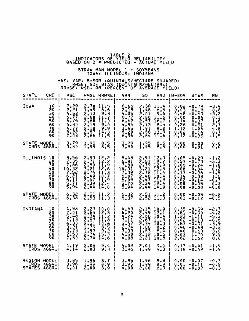
Indicators of Yield Reliability Based on D =Predicted - Actual Yield •••••••••••••••• 8

Root mean square error (RMSE) for soybeans in quintalsper hectare based on test years 1970-1979 •••••••• 9

Indicators of Yield Reliability Based on RD = 100 r.«Predicted-Actual Yield)/Actual Yield). 10

Figure 3: Percent of test years (1970-1979) the absolute value ofthe relative difference is greater than ten percent forsoybeans ••••.•• • 11

Figure 4:

Figure 5:

Figure 6:

Figure 7:

Figure 8:

Table 4:

Largest absolute value of the relative difference forsoybeans during the test years 1970-1979 •.•••.•• 12

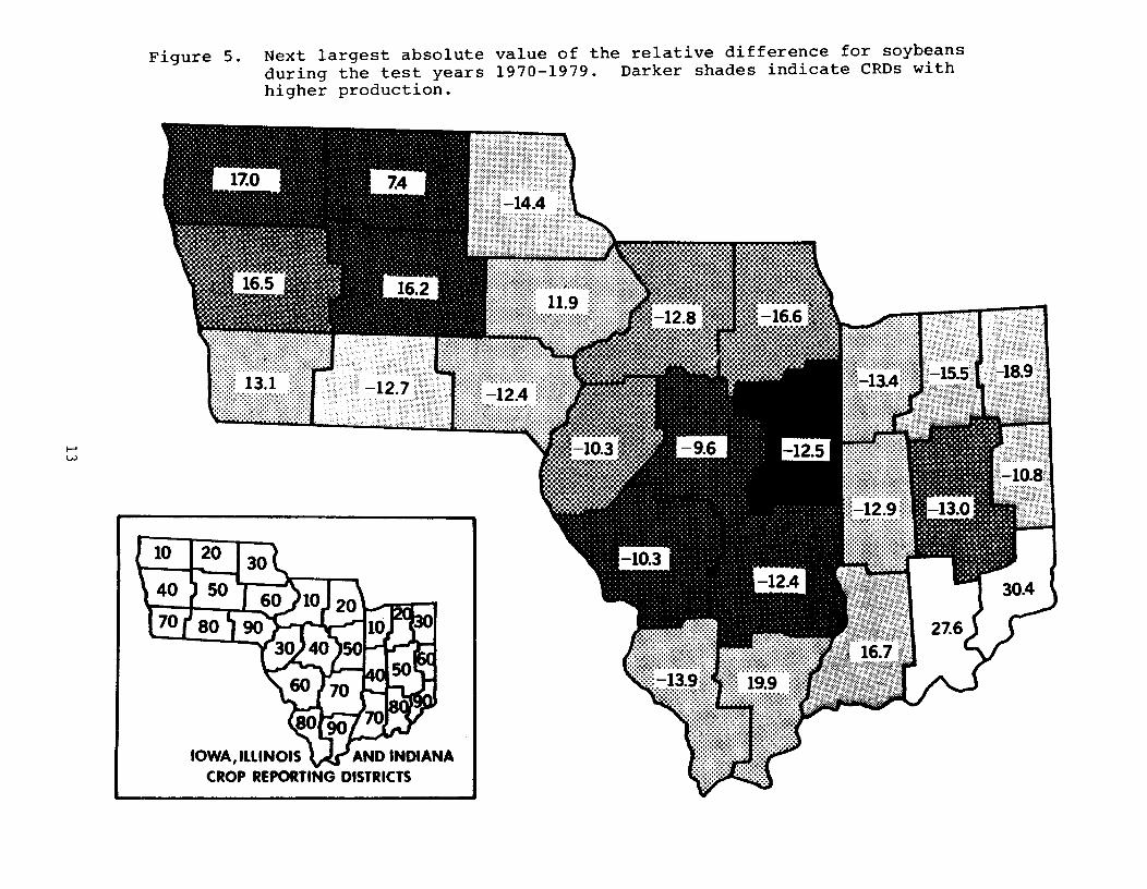
Next largest absolute value of the relative differencefor soybeans during the test years 1970-1979 •••••• 13

Iowa State Model. Actual and Predicted Yields for theTest Years 1970-1979 ••.••••.•••••• 15

Illinois State Model. Actual and Predicted Yields forthe Test Years 1970-1979 •••••••••••••• 16

Indiana State Model. Actual and Predicted Yields forthe Test Years 1970-1979 ••••.•••••••••. 17

Indicators of Yield Reliability Based on Actual andPredicted Yields •••••••••••••.•••. 18

Figure 9: Percent of test years (1970-1979) the direction ofchange in predicted yield from the previous year agreeswith the direction of change in actual soybean yield 19

Figure 10: Percent of test years (1970-1979) the direction ofchange in predicted yield from the previous three yearaverage agrees with the direction of change in actualsoybean yield •.•.•••••••••••••. 20

Figure 11: Pearson correlation coefficient between actual andpredicted soybean yields in the test years (1970-1979) • 21

Table 5: Residual Mean Square as an Indicator of the Fit of theModel Based on the Model Development Base Period •• 22

v

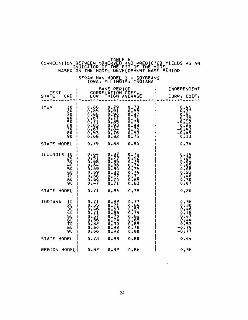
PageTable 6: Correlation Between Observed and Predicted Yields

as an Indicator of the Fit of the Model Based onthe Model Development Base Period 24

Table 7: Current Indication of Modeled Yield Reliability. 26

Figure 12: Spearman correlation coefficient between the estimate ofthe standard error of a predicted value from the baseperiod model and the absolute value of the differencebetween the predicted and actual soybean yield in thetest years (1970-1979) ....•........ 27

vi

Evaluation of "Straw Man" Modell,The Simple Linear Model,

for Soybean Yields inIowa, Illinois, and Indiana

Jeanne L. Sebaugh

SUMMARY

Straw man modell, simple linear regression of yield over time, describesa uniform increase in soybean yields over time. Indicators of yield re-liability obtained from bootstrap testing are used as a basis of comparisonbetween competing models and the results for straw man model 1 do not appearvery promising. The bias is generally small~ however, the model is unableto predict the low and high yields accurately. The model is objective,adequate, timely, simple, and not costly. However, it does not considerknown scientific relationships and does not provide a good current measureof modeled yield reliability.

DESCRIPTION OF THE MODEL

Straw Man Models Describe Technological Trends

All of the straw man models attempt to explain differences in crop yieldsover time by simply fitting trend lines to the yield data. Improvements intechnology, including varieties, hybrids, fertilizers, insecticides, herbicides,farming practices, equipment, etc., have resulted in steady improvements inyields. There are occasional set-backs, primarily due to weather, but theoverall trend has been towards increasing yields.

The straw man models demonstrate how much of the year-to-year difference inyield can be explained simply by this technological trend. These models arenot expected to be particularly accurate in predicting the yield for anyfuture year since that year's particular weather conditions are not used bythe model. However, as pointed out by Kestle (1981), these models may betreated as "below base" models. Any candidate model which cannot substantiallyoutperform a straw man model is of questionable value.

Straw Man Model 1 - Uniform Trend Over Time

Straw man model 1 is a simple linear regression over time. The statisticalmodel is E(Y) = 8 + 8lX, where Y is the soybean yield in quintals per hectareand X is the corrgsponding year number (1950=0).

The inherent assumption in a simple linear regression model is that the rateof change in the Y variable is constant over the entire range of the X values.In our case, this means that the year-to-year increases in yield are assumedto be the same later on in the time period as they were earlier. Under thatassumption, 8 is the yield in 1950 and 81 is the increase in yield betweenany two adjacgnt years in the time period being modeled.

1

EVALUATION METHODOLOGY

Eight Model Characteristics to be Discussed

The document, Crop Yie14 Model Test and Evaluation Criteria, (Wilson,et al., 1980), states:

"The model characteristics to be emphasized in theevaluation process are: yield indication reliability,objectivity, consistency with scientific knowledge,adequacy, timeliness, minimum costs, simplicity, andaccurate current measures of modeled yield reliability."

Each of these characteristics will be discussed with respect to straw manmodel 1.

Bootstrap Technique Used to GenerateIndicators of Yield Reliability

Indicators of yield reliability (reviewed below) require that the parametersof the regression model be computed for a set of data and that a yield pre-diction be made based on that data for a given "test" year. The valuesrequired to generate indicators of yield reliability include the predictedyiel~, Y, the actual (reported) yield, Y, and the difference between them,d = Y-Y, for each test year. It is desirable that the data used to generatethe parameters for the model not include data from the test year.

In order to accomplish this, the "bootstrap" technique is used. Years froman earlier base period are used to fit the model and obtain a predictionequation. The values of the independent variables for the test yearfollowing the base period are inserted into the equation and a predictedyield is generated. Then, the base period is shifted one year forward andthe process is repeated. Continuing in this way, ten (1970-1979) predictionsof yield are obtained, each independent of the data used to fit the model.

AThe Y and d values for the ten-year test period are obtained from modelsderived at the crop reporting district (CRD) level, state level. and regionlevel. Another set of Y values are obtained at the state level by using aweighted average of the predicted yields from the CRD models. Predictedyields for the region are also obtained using a weighted average of thepredicted yields from the CRD models and from the state models. The weightingfactor used is harvested acreage for the year the prediction is made.

For Illinois and Indiana, data for 1947-1969 (23 years) are used to fitprediction models for 1970, data for 1948-1970 (23 years) are used to fitprediction models for 1971, etc. For Iowa, data for 1950-1969 are used tofit prediction models for 1970 (20 years). data for 1950-1970 are used tofit prediction models for 1971 (21 years), etc. When shifting the baseperiod forward, the earliest year is dropped if it would result in more than23 years of data. A base period of consistent size is desired because ofthe type of trend models with which straw man 1 will be compared and is notnecessarily a standard bootstrap procedure.

2

The average and percent production and the yield over the ten year testperiod are listed in Table I for each geographic region. The percentageof regional production contributed by each CRD is shown graphically inFigure 1. D~rker shades indicate higher production.

Review of Indicators of Yield ReliabilityAThe Y, Y and d values for the ten-year test period at each geographic area

may be summarized into various indicators of yield reliability.A

Indicators Based on the Differences between Y and Y (d)Demonstrate Accuracy, Precision and Bias

From the d value, the mean square error (root and relative root mean squareerror), the variance (standard deviation and relative standard deviation),and the bias (its square and the relative bias) are obtained.

The root mean square error (RMSE) and the standard deviation (SD) indicatethe accuracy and precision of the model and are expressed in the originalunits of measure (quintals/hectare). It is about 68% probable that theabsolute value of d for a future year will be less than one RMSE and 95%probable that it will be less than twice the RMSE. So, accurate predictioncapability is indicated by a small RMSE.

A non-zero bias means the model is, on the average, overestimating the yield(positive bias) or underestimating the yield (negative bias). The SD issmaller than the RMSE when there is non-zero bias and indicates what theRMSE would be if there were no bias. If the bias is near zero, the SD andthe RMSE will be close in value. We prefer an unbiased model, i.e. biasclose to zero.

Indicators Based on Relative Differences between Y and Y (rd)Demonstrate Worst and Best Performance

The relative difference, rd=(IOOd/Y), is an especially useful indicator inyears where a low actual yield is not predicted accurately. This is becauseyears with small observed actual yields and large differences have the largestrd values.

Several indicators are derived using relative differences. In order tocalculate the proportion of years beyond a critical error limit, we countthe number of years in which the absolute value of the relative differenceexceeds the critical limit of 10 percent. Values between 5 and 25 percentwere investigated and a critical limit of 10 percent was found most usefulin describing model performance. The worst and next to worst performanceduring the test period are defined as the largest and next to largestabsolute value of the relative difference. The range of yield indicationaccuracy is defined by the largest and smallest absolute values of therelative difference.

3

TAB~E 1AVERAGE PRODU TION AND YIELDFOR TEST YEARS 1970-79SOYBEANS10\11 A , ILLINOIS, INDIANA

PRODUCTION (1.000) PERCENT OF" YIFLDSTATE CRD QUINTALS BUSHELS STATE REGIO~ QNTL/HA BU/ACRE~_..--_ .•._-_ ..- ---------------------------------- ----------------to\tlA 10 10,134 39.439 16.9 6.2 23.4 34.820 10,992 40.389 17.3 6.4 22.7 33.830 3.929 14.435 6.2 2.3 21.7 32.340 8.189 30.090 12.9 4.8 22.3 33.150 11,207 41,117 17.7 6.5 23.1 35.360 4.996 18.358 1.9 2.~ 24.5 36.470 5.016 18,430 7.9 2.9 22.1 32.980 3.107 11.415 4.9 1.8 20.4 30.490 5,187 19.060 8.2 3.0 23.1 34.3

STATE 63,357 232.793 36.8 22.9 34.0

ILLINOIS 10 5.670 20.834 7.5 3.3 24.0 35.620 6,960 25,575 9.2 4.0 22.2 33.030 6.331 23.263 8.4 3.7 23.5 35.040 10.855 39.885 14.4 6.3 25.0 37.250 12,870 47,288 17.1 7.5 24.2 36.060 11,412 41.931 15.1 6.6 23.2 34.670 11,739 43.133 15.6 6.8 20.8 30.980 4.800 17,637 6.4 2.8 19.2 28.690 4.694 17.248 6.2 2.7 17.4 25.8STATE 75.333 276.795 43.7 22.4 33.3

INDIANA 10 5.258 19.320 15.6 3.1 22.2 33.020 3.717 13.659 11.1 2.2 21.5 32.030 3.891 14.319 11.6 2.3 20.8 31.040 4.443 16.326 ~3.2 2.6 22.5 3~.S50 8'1°0 29.761 4.~ 4.7 23.6 3:>.160 3. 42 11.544 9. 1.8 21.0 31.270 3.304 12.139 9.8 1.9 21.0 31.380 709 2.604 2.1 0.4 18.3 27.390 1.042 3.827 3.1 0.6 18.8 27.9STATE 33,612 123,500 19.5 21.9 32.5

REGION 172.301 633.088 22.5 33.4

4

as awith higher

by CRDDarker shades

Figure 1. Production of soybeansregional total.

(1970-79 average),indicate CRDs

percent of theproduction.

IOWA, ILLINOIS AND INDIANACROP REPORTING DISTRICTS

Indicators Based on Y and Y DemonstrateCorrespondence Between Actual and Predicted Yields

Another set of indicators demonstrates the correspondence between actualand predicted yields. It would be desirable for increases in actual yieldto be accompanied by increases in predicted yields. It would also bedesirable for large (small) actual yields to correspond to large (small)predicted yields.

Two indicators relate the change in direction of actual yields to thecorresponding change in predicted yields. One looks at change from theprevious year (nine observations) and the other at change from the averageof the previous three years (seven observations). A base period of threeyears is used since a longer base period would further decrease the numberof observations, while a shorter period would not be very different from thecomparison to a single previous year.

Finally, the Pearson correlation coefficient, r, between the set of actualand predicted values for the test years is computed. It is desirable thatr(-l ~ r ~ +1) be large and positive. A negative r indicates smaller pre-dicted yields occurring with larger observed yields (and vice versa).

Current Measure of Modeled Yield ReliabilityDefined by a Correlation Coefficient

One of the model characteristics to be evaluated is its ability to providean accurate, current measure of modeled yield reliability. Although aspecific statistic was not discussed in the paper, Crop Yield Model Testand Evaluation Criteria, (Wilson, et al., 1980), it was stated that:

"This 'reliability of the reliability' characteristiccan be evaluated by comparing model generated reliabilitymeasures with subsequently determined deviation betweenmodeled and 'true' yield."

For regression models, this suggests the use of a correlation coefficientbetween two variables generated for each test year. One variable is anindicator of the precision with which a prediction for the next year canbe made, based on the model development base period. The other variable(obtained retrospectively) is an indicator of how close the predicted valuefor the next year actually is to the "true" value. The estimate of thestandard error of a predicted value from the base period model is used forthe first value, Sy, and the absolute value of the difference between thejredicted and actual yield in the test year is used as the second variable,

d I.A non-parametric (Spearman) correlation coefficient, r, is employed since theassumption of bivariate normality cannot be made. A positive value ofr(-l ~ r ~ +1) indicates agreement between Sy and Idl, i.e., a smaller (larger)value of sf is associated with a smaller (larger) value of Idl. An r valueclose to +1 is desirable since it indicates that a small standard error ofprediction (and therefore a narrow confidence interval about the true predictedvalue) is associated with small discrepancies between predicted and actualyields. If this were the case, one would have confidence in Sy as an indicatorof the accuracy of Y.

6

MODEL EVALUATION~Indicators of Yield Reliability Based on Differences between Y and Y (d) Show

Small Bias and a Standard DeviationBetween 1~~3~ Quintals/Hectare

The CRD, state and region values of indicators of yield reliability basedon d for this simple linear model are given in T~b1e 2. The bias forCRDs is generally less than half a quintal in Iowa and Illinois and lessthan a quintal in Indiana. The CRDs in Iowa and Illinois have a relativebias of less than five percent. In Indiana, three CRDs have a relativebias between five and ten percent, while the rest are less than fivepercent.

The root and relative root mean square error values (RMSE and RRMSE) aresomewhat lower in Iowa and higher in Illinois, as can be seen for theRMSE values in Figure 2. CRD values for RMSE range from 1.49 to 3.21quintals/hectare and values for RRMSE range from 6.6 percent to 15.0percent.

Generally, as the level of aggregation increases in size, the bias becomescloser to zero and the RMSE becomes smaller. This demonstrates the greateraccuracy obtained with the data which has been stabilized through theaggregation process. The results are very similar regardless of whetherthe aggregation is done prior to fitting the model (state and region models)or after the models are fit (CRDs aggregated and states aggregated).

Indicators of Yield Reliability Based on Relative DifferencesBetween3 and Y (rd) Show 1974 as Worst Year and

20-40 Percent of the Years Have rd .Greater than 10 PercentThe CRD, state, and region values for indicators of yield reliabilitybased on rd are given in Table 3. CRD values are also shown in Figure3-5. Two to four of the ten test years have abso1ute,re1ative differencesgreater than 10 percent in most (21 out of 27) of the CRDs (Figure 3).The very low yield in 1974 caused the largest absolute relative differencein most CRDs, ranging from 15.8 percent to 57.4 percent (Figure 4). Therange in values for the next largest absolute relative difference is 7.4percent to 30.4 percent (Figure 5). The smallest absolute relative dif-ference is sometimes zero (four CRDs) and ranged up to 3.3 percent. Thesesmall absolute relative differences result in the range being very much likethe largest absolute relative difference varying over CRDs from 14.9 percentto 55.4 percent.

As compared to the CRD results, the state and regional aggregate values forthe largest and smallest absolute relative difference are somewhat lower.There are fewer years with absolute relative differences greater than 10percent. The method of aggregation makes little difference.

7

TAB~E 2INDICATORS Of Y E~D REXIABILITYBASED ON D = P~EDICT D - CTUAL YIELDSTRAw MAN MODE~ 1 - SOY8EA~SIOWA. ILLI~ IS. INDIANA

MSE. VAR, 8-SQR (QUINTAyS/HECTARE SQUARED)RMSE. SO, BIAS ~QU NTALS/HECTARE)RRMSE. ~SD. RB (PER E~T Of AVERAGE YJEL~)STATE CRD I MSE RMSE RRM<;E VAR SO RSD IB-SQR BIAS RB-~-~------~-I------------------------------------1-----------------I 7.29 IIOWA 10 I 2.70 11.S 6.66 ?58 11.4 I 0.62 -0.79 -3.420 I 2.21 1.49 6.6 2.18 1.48 6.5 I 0.03 0.18 0.830 I 4.52 2.13 9.8 4.05 2.01 9.6 I 0.48 -0.69 -3.240 6.77 2.60 p.7 6.77 2.69 11.6 I 0.00 0.06 0.350 6.76 2.60 1.0 6.62 2.5 10.7 I 0.14 0.31 1.660 4.80 2.19 9.0 4.54 2.13 8.5 0.26 0.51 2.170 4.77 2·A8 9.9 3.65 1.91 8.2 1.12 1.06 4.880 8.22 2. 7 14.0 8.20 2.86 13.9 0.02 0.14 0.790 7.08 2.66 11.S 6.96 2.64 11.6 0.12 -0.35 -1.5STATE MOOEb 3.79 1.95 8.5 3.79 1.95 8.5 0.00 0.00 0.0CRDS AGG • 3.80 1.95 8.5 3.80 1.95 8.5 0.00 0.01 0.0

ILLINOIS 10 8.56 2.93 12.2 8.48 2.91 12.3 0.08 -0.29 -1.220 7.35 2.71 12.2 6.81 2.6~ 12.2 0.53 -0.73 -3.330 7.86 2.80 11.9 7.80 2.7 12.0 0.06 -0.24 -1.040 10.32 3.21 12.8 10.31 3.21 12.8 0.00 0.04 0.250 7.52 2.74 11.3 7.39 2.72 11.4 0.13 -0.36 -1.560 6.21 2.49 10.7 6.07 2.46 10.4 0.14 0.38 1.670 6.11 2.47 1~.9 6.09 2.47 11.9 0.02 -0.14 -0.180 5.71 2.39 1 .4 5.70 2.39 12.4 0.00 0.05 0.390 5.94 2.44 14.0 5.94 2.44 14.0 0.00 -0.00 -0.0STATE MODEL 6.32 2.51 11.2 6.32 2.51 11.2 0.00 -0.05 -0.2CRDS AGG~. 6.38 2.53 11.3 6.37 2.52 11.3 0.01 -0.12 -0.5

INDIANA 10 4.98 2.23 10.0 4.63 2.15 10.0 0.35 -0.59 -2.720 7.01 2.65 12.3 6.20 2.49 12.1 0.81 -0.90 -4.230 5.48 2.34 11.2 4.24 2.06 10.4 1.23 -1.1~ -5.340 7.~3 2.67 11.8 7.11 2.67 11.9 0.02 -0.1 -0.650 6. 0 2.51 10.6 5.47 2.34 10.3 0.83 -0.91 -3.960 3.21 1.79 8.5 2.74 1.66 8.2 1).46 -0.68 -3.270 3.73 1.93 9.2 3.33 1.83 8.4 0.40 0.61 3.080 7.53 2.74 15.1) 4.50 2.12 10.6 3.03 1.74 9.590 1.50 2.74 14.6 4.88 2.21 10.8 2.62 1.62 8.6STATE MOI)EL 4.19 2.05 9.4 4.02 2.01 9.4 0.17 -0.41 -1.9C~DS AGG~. 4.14 2.03 9.1 3.96 1.99 9.3 0.18 -0.42 -1.9

REGION MODEL 3.85 1.96 8.7 3.85 1.96 8.8 0.00 -0.01 -0.3CRDS AGGR. 3.96 1.99 8.9 3.95 1.99 8.9 0.01 -0.11 -0.5STATES AGG~. 4.01 2.00 8.9 4.00 2.00 8.9 0.00 -0.01 -0.3

8

Root meanon test yearsproduction.

Figure 2. square error (RMSE) for soybeans in quintals per1970-1979. Darker shades indicate CRDs with

hectarehigher

based

10 20

80 90IOWA, ILLINOIS AND INDIANA

CROP REPORTING DISTRICTS

TABTE 3BASED ON RD INDICATORS OF Y ELD RELIABI~ITY= 00 ~ «PREDICTED-ACTUAL YI_LO)/ACTUAL yIELD)

STQAW MAN MODEL 1 - SOYBEA'4SIOWA, ILLINOIS. INOIA~APERCEI\JT

OF YEARS LARGEST ~RDI 'JEXT SMALbE<;T QANGESTATE CRD I P~DI>10% RO (Y AQ) LA~GEST IR I IROI-----~------,---------- -------------- --------- ---------- ------IOWA 10 60 -17.4 (1972 ) 17.0 1.2 16.220 10 19.6 (1974 ) 7.4 -0.4 19.130 40 15.8 (1974 ) -14.4 -1.0 14.940 40 25.4 (1976 ) 16.5 0.0 25.450 40 28.0 (1974) 16.2 0.4 27.560 20 27.1 (1974 ) 11.~ 0.4 26.770 30 26.5 (}974) 13.1 -1.3 25.280 20 57.4 (}971+) -12.7 2.0 55.4

90 20 38.1 (1974 ) -12.4 -0.4 31.7STATE MODEL 20 23.9 (}974) 12.5 -0.4 23.5

Cf~DS AGGR. 20 23.9 (1974) 12.5 0.0 23.9

ILLINOIS 10 40 41.2 (}914) -12.8 -0.4 40.820 40 26.5 (1974) -16.6 0.0 26.530 20 42.8 (1974 ) -10.3 2.1 40.640 10 52.7 (1974 ) -9.6 0.8 51.950 40 36.9 (1974 ) -12.5 1.2 35.760 20 34.3 (1974) -10.3 -3.3 31.070 40 36.8 (1974 ) -12.4· 0.0 36.880 50 26.6 (1974 ) -13.~ -1.1 25.590 50 26.6 (1914) 19.9 -1.1 25.0

STATE MODEb 20 31.6 (1914) -10.~ 1.9 35.1CRDS AGG • 30 31.0 (1974) -11.7 1.9 35.0

II\JOIANA ~8 40 25.4 (1974) -13.4 1.3 24.140 31.0 (1974 ) -15.5 2.0 29.030 30 24.5 (1974) -18.~ -0.5 24.140 20 48.1 (1974) -12.9 -0.4 47.650 30 28.2 (1974 ) -13.0 -2.7 25.560 20 18.6 (1974 ) -10.8 -1.0 17.770 20 22.6 (1974 ) 16.7 0.5 22.180 40 33.Q (1975 ) 27.6 0.0 33.890 40 33.1 (1913) 30.4 3.0 30.1STATE MODEL 20 28.0 (1974) -12.0 0.0 28.0

CRDS AGGR. 20 28.0 (1974 ) -11.6 -0.5 27.5

REGION MODEL 10 29.9 (}974) -8.1 -0.9 28.9CRDS AGGR. 10 29.9 (1914 ) -8.5 -0.9 28.9STATES AGGR. 10 30.5 (1914) -8.1 -0.9 29.5

10

test years (1970-1979) the absolutegreater than ten percent forwith higher production.

Figure 3. Percent ofdifference isindicate CRDs

valuesoybeans.

of the relativeDarker shades

10 20

80 90rOWA, rlUNOrS AND INDIANA

CROP REPORTING DrSTRrCTS

soybeanswith higher

Figure 4. Largest absolute valuetest years 1970-1979.

of theDarker

relative difference forshades indicate CRDs

during theproduction.

80 90IOWA, ILLINOIS AND IND'ANA

CROP REPORTING DISTRICTS

•.....N

the relative differenceDarker shadesFigure 5. Next largest absolute

during the test yearshigher production .

value of1970-1979.

for soybeansindicate CRDs with

•......w

10 20

80 90IOWA, ILLINOIS AND INDIANA

CROP REPORTING DISTRICTS

~ Indicators of Yield Reliability Based OnY and Y Show Low Correspondence Between the Direction of

Change in Predicted as Compared to Actual Yields

Plots of the actual and predicted yields over the ten-year test period usingstate level models are displayed in Figures 6, 7 and 8. The CRD, state andregion values for indicators of yield reliability based directly on actualand predicted yields are given in Table 4. CRD values are also shown inFigures 9-11.

The results for this model are poor. In only 3 out of 27 CRDs does the changein direction of predicted yields agree with the change in direction of actualyields from the previous year in over half of the test years (Figure 9). Whenthe direction of change is based on an average of the three previous years,the direction of change is in agreement over half the time in only 10 of the 27CRDs (Figure 10). Results are not much better at the state or region level.The Pearson r is negative for five of the CRDs (Figure 11). The largest posi-tive r is 0.53. State and region results are not much better. This indicatesthat the model does a poor job of predicting high and low yields.

Change of predicted yield from previous forecasts within the current yearcannot be investigated with a straw man model since the prediction for thecurrent year only requires the addition of the actual yield for the previousyear. No additional forecasts are made during the growing season unlessmore accurate figures for yield in previous years become available.

Base Period Indicates More Precision ThanIndependent Tests Can Confirm

Certain statistics generated from the regression analysis of the base perioddata are often used to provide some indication of expected yield reliability.However, these statistics only reflect how well the model describes thedata used to generate the model, i.e., fit of the model, rather than howwell the model can predict given new data. Therefore, it is important tocompare these indicators of fit of the model to the independent indicatorsof yield reliability discussed in the preceding sections. In this way, onecan see how these base period indicators of fit of the model do or do notcorrespond to independent test indicators of yield reliability.

One indicator of yield reliability, the mean square error (MSE) , is the sumof squared d values (d = Y - Y) for the independent test years divided by thenumber of test years (Table 2). The direct analogue for the model develop-ment base period is the residual mean square. The residual mean square isobtained by first generating the usual least squares prediction equationusing the base period years. Then instead of predicting the yield for thefollowing test year, yields are predicted for each of the base period years.The residual mean square is the sum of squared d values for these base periodyears divided by the appropriate degrees of freedom (number of years minusnumber of parameters estimated in fitting the model). Whereas one value ofMSE is generated for each geographic area over the entire test period, a valueof the residual mean square is generated for each base period corresponding toa test year in that area. The low, high, and average of the base period valuesfor each area are given in Table 5.

14

FIGURE 6IOWA

State ModelActual and Predicted Yields for

the Test Years 1970-1979

STQAWMAN MODEL 1

A = ACTUAL yIELD

SIMPLE LIN~AR REGRFSSrO~SOYBEA\JSP = PREDICTED YtELO

YIELD

27262S24

232221201918171615

IIII+I+I+I+I+I+I+I+I+I+I+I+I+IIII--~+~---+----+----+----+----+----+----+----.----.-~1~70 1971 1972 1973 1974 1975 1q76 1977 1978 1979

YEAR

15

FIGURE 7ILLINOIS

State ModelActual and Predicted Yields for

the Test Years 1970-1979

ST~AwMA~ MODEL 1

A. = ACTUAL vIEL~

SI~~LE LI~EAR REGRfSSTn~SOYBEA\JSP = PREDICTED YTELD

24

27

26

25

2322212019

18

17

1615

YIELD IIII

+I+I+I+I+I

+I+I+I+I+t+I+I+I,II---+----+----+----+----+----+----+----+----+----+--1970 lY71 1972 1973 1974 1975 1976 1977 1978 1979

YEAR

16

ST~AWMA~ M~DEL 1

.p--~_ .... -..P- - -

..p... - - -

YIELD

272625242322212019lR171615

FIGURE 8INDIANA

State ModelActual and Predicted Yields for

the Test Years 1970-1979

- SIMPLE LI~EAR REGRESSJO~SOY8EA~SA = ACTUAL vIELD P = PREDICTED YIELD

IIII•I•I•I•I•I•I•I•I•I•I•,•,•I,,,---+----+----.----+----+----+----+----+----+----+--1970 1971 1912 1973 1974 1975 1976 1917 1918 1919

YEAR

17

TAB~E 4NDICATORS OF Y ELD RE IA91LITYBAStD ON ACTUAL AN PREDI~TED YIELDSSTRAW MAN MODEb 1 - SOYBEA~SIOWA. ILLIN IS. I~DIA~A

J PERC~NT OF YEAR~DIQECT ON 0 CHAN E IS CORQE T pEARSONSTATE CRD FROM PREvious YEARI ~ROM BASE ~~RIOD CORR. COEF.-----·-------I-------~~---------- ------------------ ----~----_.•-

~8I 22 I~IOWA I 0.46

~~0.31

30 I 0.5140 I 22 51 0.38SO I

~~43 .0.12

60 I 43 0.2570 22 43 -0.4380 56 29 -0.4990 44 57 0.13

STATE MODEL 22 71 0.34CROS AGGR. 22 71 0.33

ILLINOIS 10 22 29 0.1420 11 43 0.2830 33 43 0.0440 33 43 0.05SO 33 43 0.0860 11 43 0.2370 44 43 0.4880

~~29 0.30

90 29 0.01STAT5 MOOE~ II 43 0.20

CR S AGG • 43 0.19

INDIANA ~g 44 43 0.3633 57 0.30

30 56 57 0.4840 56 57 0.18SO 44 57 0.4760 33 71 0.4470 33 29 0.5380 22 29 .0.7490 33 0 .0.71

STATE MODE~ 56 57 0.44CRDS AGG • 56 51 0.45

REGION MODEL 44 57 0.38CROS AGGR. 33 51 0.35

STATES AGGR. 33 51 0.33

18

Figure 9. Percent of test years (1970-1979) the direction of change in predictedyield from the previous year agrees with the direction of change in actualsoybean yield. Darker shades indicate CRDs with higher production.

IOWA,IUINOIS AND INDIANACROP REPORTING DISTRICTS

in predictedthe direction of

CRDs with higher

Figure 10. Percent of test years (1970-1979) the direction of changeyield from the previous three year average agrees withchange in actual soybean yield. Darker shades indicateproduction.

8090IOWA, ILLINOIS AND INDIANA

CROP REPORTING DISTRICTS

No

between(1970-1979). Darker

Figure 11. Pearson correlation coefficientyields in the test yearswith higher production .

actual and predicted soybeanshades indicate CRDs

.•....•.....•••....•.•.•.•....•.•.•.•.•.•.•....•.•....•.::=:=:=::::::::::::::::::::: .......', ........•..•..•...•.•.•.•...........•...•.•.•...............................:::::::::::::::::::::::::::::::::.

TABLE 5ReSIDUAL ~EAN SQUAR~ AS ANIND I .ATOR OF THE F' IT 0 THE ~oD:::lBASED ON THE MODEL DEVELOPMENT BASE oEqIODSTQAW MAN MODEL 1 - SOYBEANSIOWA, ILLINOIS. INDIANA

BASE PERIOD I'JDEPENDENTRESIDUAL MEAN SQUARE TESTSTATE CRD LOW HIGH AVERAGE ~SE--_ .._-----~- -------------------------- ------ ..--------IOwA 10 4.49 5.91 5.24 7.2920 1.18 2.18 2.02 2.2130 1.15 2.56 2.12 4.5:2

40 4.50 5.39 4.87 F-..7150 2.15 4.20 3.40 6.7660 1.50 2.17 2.10 4.8070 3.05 4.36 3.94 4.1780 3.60 5.94 4.61 8.2290 2.61 4.38 3.33 7.0A

STATE ~ODEL 2.07 2.89 2.45 3.79

ILLINOIS 10 1.31 3.84 2.57 8.5620 1.56 3.57 2.44 7.3530 1.19 3.71 2.91 7.8640 1.90 5.23 3.56 10.3250 1.67 4.08 2.87 7.5260 3.36 4.65 3.91 6.2170 3.59 4.96 4.24 6.1180 3.57 6.83 5.60 5.7190 3.33 4.77 4.09 5.94STATE MODEL 1.83 3.42 2.65 6.32

INDIANA 10 1.93 3.09 2.51 4.9820 2.12 4.25 3.04 7.0130 2.40 3.75 2.94 5.4940 2.17 4.53 3.35 7.1350 2.86 5.14 3.85 6.3060 3.32 3.87 3.65 3.2170 2.11 3.25 2.63 3.7380 1.81 4.53 2.95 7.5390 2.07 4.19 3.26 7.50,

STATE MODEL I 1.55 2.92 2.16 4.19IIREGION MODEll 1.00 2.10 1.51 3.85

22

The MSE values in Table 2 are also given in Table 5. The average residual meansquare is almost always less than the MSE, many times being less than half aslarge. In fact, the largest residual mean square is almost always less than theMSE. Therefore, the results from the independent test indicate less reliabilitythan one might have expected from base period model development results.

Another indicator of yield reliability is the correlation coefficient, r, be-tween the observed and predicted yields for the independent test years (Table 4).It is desirable for r to be close to +1, even though it can be negative. Theanalogue for the model development base period is the square root of R2, thecoefficient of multiple determination. The square root of R2 expressed as aproportion, R (0 ~ R ~ 1), may be interpreted as the correlation between ob-served and predicted values for the base period years. The low, high, andaverage values of R for each geographic area are given in Table 6.

The Pearson correlation coefficient values in Table 4 are also given in Table 6.The highest positive value of r is 0.53 and some r values for negative. AverageCRD values of R range from 0.57 to 0.88. The values of r from the independenttests are certainly much lower than the values of R from the base period. It isobvious that levels of R (or alternatively R2) for a model development baseperiod are of no value in indicating independent performance of this model. Infact, the base period R or R2 can be very misleading.

Model is Objective

Since the single independent variable is objectively defined (year minus 1950),no subjective inputs are required to run the model.

Results might differ if the set of years used to generate the models were changed.In this evaluation, the post World War II period was used, resulting in amaximum of twenty-three years on which to base the model (1947-1969, 1948-1970,etc.). Iowa had some slightly shorter periods since comparably defined yieldswere not available until 1950.

Once the decisions on the time period to use for model development and on theregression method to use (least squares) are fixed, the operation becomescompletely objective.

Model Does Not Consider Known Scientific Relationships

The straw man models do not consider factors which have a recognized causal re-lationship with crop yields. For example, it is well known that year-to-yearvariations in weather have an important effect on yield. Therefore, if weatherdata were available, it would be consistent with scientific knowledge to includeweather variables in a model predicting crop yields. Weather variables are ex-cluded from the straw man models yet nothing is done to account for the factthat the yields have been influenced by weather. The yields may also have beeninfluenced by other non-technology factors. However, since no adjustment ismade to the yields for these non-technology factors and since these factorsare not included as independent variables in the model, the straw man modelresults will be affected by non-technology influences. As was anticipated, thecalculated slope of the regression line for straw man model 1 is positive foreach base period at each geographic location.

23

TABbE 6CORRELATIO~ BETWEE~ OB~ERVE ~~D PREDICTED YIELDS AS A~INDICATOR OF THE FIT OF THE MODE~BASED ON THE MODEL DEVELOPMENT BASE ~ ~IOD

STRAw MAN MODE~ 1 - SOYBEANSIOWA. ILLIN IS. INDIANABAc;E PERIOD I I\JI)EPE~DENT

TEST CORRELATAON COEFG ,STATE CRD LOW HI H AVEQA E , CORR. COEF.-----------. --------------------------t---------------IOwA 10 0.66 0.79 0.73 0.46~o 0.8~ 0.91 0.88 0.3130 0.85 0.90 0.81 0.5140 0.b7 0.71 0.71 0.3850 0.11 0.85 0.78 -0.~260 0.83 0.93 0.88 o. 570 0.67 0.84 0.76 -0.4380 0.53 0.76 0.63 -0.4990 0.68 0.82 0.75 0.13STATE MODEL 0.79 0.88 0.84 0.34

ILLI!\JOIS10 0.64 0.87 0.75 0.1420 0.51 0.72 0.62 0.2830 0.68 0.85 0.75 0.0440 0.64 0.86 0.74 0.0550 0.69 0.84 0.76 0.0860 0.69 0.80 0.74 0.2370 0.66 0.77 0.71 0.4880 0.60 0.74 0.68 0.3090 0.47 0.71 0.63 0.07STATE MODEL 0.71 0.86 0.78 0.20

INDIANA 10 0.71 0.82 0.77 0.3620 0.55 0.71 0.64 0.3030 0.46 0.69 0.57 0.4840 0.71 0.86 0.79 0.1850 0.57 0.70 0.65 0.4760 0.56 0.74 0.65 0.4470 0.82 0.90 0.85 0.5380 0.60 0.92 0.78 -0.7490 0.b6 0.92 0.80 -0.77

STATE MODEL 0.73 0.85 0.80 0.44

REGION MODEL 0.82 0.92 0.86 0.38

24

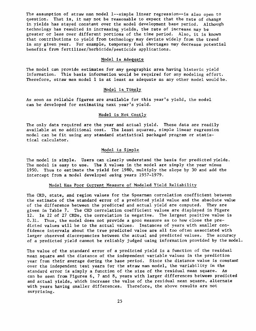
The assumption of straw man model l--simple linear regression--is also open toquestion. That is, it may not be reasonable to expect that the rate of changein yields has stayed constant over the model development base period. Althoughtechnology has resulted in increasing yields, the rate of increase may begreater or less over different portions of the time period. Also, it is knownthat contributions to yield from technology may deviate widely from the trendin any given year. For example, temporary fuel shortages may decrease potentialbenefits from fertilizer/herbicide/pesticide applications.

Model is Adequate

The model can provide estimates for any geographic area having historic yieldinformation. This basis information would be required for any modeling effort.Therefore, straw man model 1 is at least as adequate as any other model would be.

Model is Timely

As soon as reliab~e figures are available for this year's yield, the modelcan be developed for estimating next year's yield.

Model is Not Costly

The only data required are the year and actual yield. These data are readilyavailable at no additional cost. The least squares, simple linear regressionmodel can be fit using any standard statistical packaged program or statis-tical calculator.

Model is Simple

The model is simple. Users can clearly understand the basis for predicted yields.The model is easy to use. The X values in the model are simply the year minus1950. Thus to estimate the yield for 1980, multiply the slope by 30 and add theintercept from a model developed using years 1957-1979.

Model Has Poor Current Measure of Modeled Yield Reliability

The CRD, state, and region values for the Spearman correlation coefficient betweenthe estimate of the standard error of a predicted yield value and the absolute valueof the difference between the predicted and actual yield are computed. They aregiven in Table 7. The CRD correlation coefficient values are displayed in Figure12. In 22 of 27 CRDs, the correlation is negative. The largest positive value is0.31. Thus, the model does not provide a gooa measure as to how close the pre-dicted values will be to the actual values. Instances of years with smaller con-fidence intervals about the true predicted value are all too often associated withlarger observed discrepancies between the actual and predicted values. The accuracyof a predicted yield cannot be reliably judged using information provided by the model.

The value of the standard error of a predicted yield is a function of the residualmean square and the distance of the independent variable values in the predictionyear from their average during the base period. Since the distance value is constantover the independent test years for the straw man model, the variability in thestandard error is simply a function of the size of the residual mean square. Ascan be seen from Figures 6, 7 and 8, years with larger differences between predictedand actual yields, which increase the value of the residual mean square, alternatewith years having smaller differences. Therefore, the above results are notsurprising.

25

TABgE 7CURRENT IN ICATION OfMODELED YIEL REL ABILITYAGREE~ENT BETWEEN BASE PERIOD PREDICTEDAND TEST YEAR ACTUAL ACCURACY

STRAW MAN MODEL 1 - SOYBEANSIOWA. ILLINOIS. INDIANASPEARMANSTATE CRD CO~RELATION COEf.------------.---- -----------~----------~

IOWA 10 -0.15cO 0.1630 -0.08••0 -0.3250 0.3160 -0.0570 -0.5980 -0.7090 -0.62

STAT& ~~gEQ -8·~8CR S G. - • 1

ILLINOIS 10 -0.0420 0.1230 -0.48••0 -0.3650 -0.6~60 -0.670 -0.1180 -0.6290 -0.71

STATE -..ODEL -0.30CRDS AGGQ. -0.15

INDIANA 10 -0.33C:?O 0.0930 -0.16••0 -0. 050 -0.0600 -0.7870 -0·!3ijO -0.90 0.0

STATE "'OOE~ -0.2~CROS AGG • 0.0

REGION MOOEL -0.18CRDS AGGQ. o. 7STATES AGG~. 0.02

26

coefficient between the estimate of the standardthe base period model and the absolute

predicted and actual soybean yield in the testshades indicate CRDs with higher production.

Figure 12. Spearman correlationof a predicted value fromthe difference between theyears (1970-79). Darker

errorvalue of

IOWA, ILLINOIS AND INDIANACROP REPORTING DISTRICTS

CONCLUSIONS

Straw man modell, simple linear regression of yield over time, describesa uniform increase in soybean yields over time. Indicators of yield re-liability obtained from bootstrap testing are used as a basis of comparisonbetween competing models and the results for straw man model I do not appearvery promising. The bias is generally small, however, the model is unableto predict the low and high yields accurately. The model is objective,adequate, timely, simple, and not costly. However, it does not considerknown scientific relationships and does not provide a good current measureof modeled yield reliability.

In conclusion, as expected, straw man model 1 is truly a "below base" model.Competing models, requiring additional inputs, will certainly be less simpleand more costly, will probably be less timely, and will possibly be lessadequate and objective. However, it is hoped that these models will pro-vide more accurate indicators of yield reliability and current measures ofmodeled yield reliability.

28

REFERENCES

KESTLE, RICHARD A., 1981. Analysis of Crop Yield Trends and Developmentof Simple Corn and Soybean "Straw Man" Models for Indiana, Illinois, andIowa. AgRISTARS Yield Model Development Project, Document YMD-2-1l-l(80-11.1). ESS Staff Report AGESS8l0ll4.

WILSON, WENDELL W., BARNETT, THOMAS L., LeDUC, SHARON K., WARREN, FRED B.,1980. Crop Yield Model Test and Evaluation Criteria. AgRISTARS YieldModel Development Project, Document YMD-1-1-2 (80-2.1).

29