evaluation of the dc opportunity scholarship program ... · evaluation of the dc opportunity...
TRANSCRIPT

Evaluation of the DC Opportunity Scholarship Program: Impacts After One Year
Evaluation of the DC Opportunity Scholarship Program:
Impacts After One Year
Patrick Wolf, Principal Investigator, University of Arkansas Babette Gutmann, Project Director, Westat
Michael Puma, Chesapeake Research Associates Lou Rizzo, Westat
Nada Eissa, Georgetown University
Marsha Silverberg, Project Officer, Institute of Education Sciences
Institute of Education Sciences National Center for Education Evaluation and Regional Assistance NCEE 2007-4009 U.S. Department of Education June 2007
U.S. Department of Education Margaret Spellings Secretary Institute of Education Sciences Grover J. Whitehurst Director National Center for Education Evaluation and Regional Assistance Phoebe Cottingham Commissioner June 2007 This report was prepared for the Institute of Education Sciences under Contract No. ED-04-CO-0126. The project officer was Marsha Silverberg in the National Center for Education Evaluation and Regional Assistance. IES evaluation reports present objective information on the conditions of implementation and impacts of the programs being evaluated. IES evaluation reports do not include conclusions or recommendations or views with regard to actions policymakers or practitioners should take in light of the findings in the reports. This report is in the public domain. While permission to reprint this publication is not necessary, the citation should be: Wolf, Patrick, Babette Gutmann, Michael Puma, Lou Rizzo, Nada Eissa, and Marsha Silverberg. Evaluation of the DC Opportunity Scholarship Program: Impacts After One Year. U.S. Department of Education, Institute of Education Sciences. Washington, DC: U.S. Government Printing Office, 2007. To order copies of this report,
• Write to ED Pubs, Education Publications Center, U.S. Department of Education, P.O. Box 1398, Jessup, MD 20794-1398.
• Call in your request toll free to 1-877-4ED-Pubs. If 877 service is not yet available in your area, call 800-872-5327 (800-USA-LEARN). Those who use a telecommunications device for the deaf (TDD) or a teletypewriter (TTY) should call 800-437-0833.
• Fax your request to 301-470-1244. • Order online at www.edpubs.org.
This report also is available on the Department’s website at http://ies.ed.gov/ncee. Upon request, this report is available in alternate formats such as Braille, large print, audiotape, or computer diskette. For more information, please contact the Department's Alternate Format Center at 202-260-9895 or 202-205-8113.
iii
Acknowledgments
This report is the third of a series of annual reports, as mandated by Congress. We gratefully acknowledge the contributions of a significant number of individuals in its preparation and production.
Staff from the U.S. Department of Education and the District of Columbia Mayor’s Office
provided ongoing support throughout the process. Guidance and comments were received from Ricky Takai, Associate Commissioner of the Institute of Education Sciences’ (IES) National Center for Education Evaluation (NCEE) and director of its evaluation division, and Phoebe Cottingham, Commissioner of NCEE. Michelle Armstrong, John Fiegel, and Margo Anderson of the Office of Innovation and Improvement served as important liaisons with the Washington Scholarship Fund.
Staff from the Washington Scholarship Fund provided helpful information and have always
been available to answer our questions. We are also fortunate to have the advice of an Expert Advisory Panel. Members include:
Julian Betts, University of California, San Diego; Thomas Cook, Northwestern University; Jeffrey Henig, Columbia University; William Howell, University of Chicago; Guido Imbens, Harvard University; Rebecca Maynard, University of Pennsylvania; and Larry Orr, Abt Associates.
The challenging task of assembling the analysis files was capably undertaken by Yong Lee,
Quinn Yang, and Yu Cao at Westat. Additional superb analysis support was provided by Brian Kisida at the University of Arkansas and Peter Schilling at Westat. The management and conduct of the data collection was performed by Juanita Lucas-McLean, Kevin Jay, and Sabria Hardy of Westat. Expert editorial and production assistance was provided by Evarilla Cover and Saunders Freeland of Westat. Administrative support for the Georgetown University project activities was provided ably by Stephen Cornman.
iv
Disclosure of Potential Conflicts of Interests1
The research team for this evaluation consists of a prime contractor, Westat, and two subcontractors, Dr. Patrick Wolf (formerly at Georgetown University) and his team at the University of Arkansas Department of Education Reform and Chesapeake Research Associates (CRA). None of these organizations or their key staff has financial interests that could be affected by findings from the evaluation of the DC Opportunity Scholarship Program (OSP). No one on the seven-member Expert Advisory Panel, convened by the research team once a year to provide advice and guidance, has financial interests that could be affected by findings from the evaluation.
1 Contractors carrying out research and evaluation projects for IES frequently need to obtain expert advice and technical
assistance from individuals and entities whose other professional work may not be entirely independent of or separable from the particular tasks they are carrying out for the IES contractor. Contractors endeavor not to put such individuals or entities in positions in which they could bias the analysis and reporting of results, and their potential conflicts of interest are disclosed.
v
Contents
Page
Executive Summary ...................................................................................................................................xiii 1. Introduction...................................................................................................................................... 1
1.1 The DC Opportunity Scholarship Program......................................................................... 1 1.2 The Mandated Evaluation ................................................................................................... 3 1.3 Contents of This Report ...................................................................................................... 5
2. Early Implementation of the Program and the Sample for the Impact Analysis.............................. 7
2.1 Student Recruitment ........................................................................................................... 7 2.2 The OSP Lotteries and the Creation of the Impact Sample ................................................ 8
Lottery Design and Outcomes ............................................................................................ 9 Creation of the Impact Sample ......................................................................................... 10
2.3 Characteristics of the Impact Sample ............................................................................... 12
Overall Sample ................................................................................................................. 12 Treatment vs. Control Groups........................................................................................... 14
2.4 Schools Attended by OSP Applicants............................................................................... 15
Characteristics of All Participating Schools ..................................................................... 15 Characteristics of Participating Schools Attended by the Impact Sample........................ 17
3. Research Methodology .................................................................................................................. 23
3.1 The “Treatment” and the “Counterfactual” ...................................................................... 23 3.2 Study Power...................................................................................................................... 24 3.3 Sources of Data, Outcome Measures, and Baseline Covariates........................................ 25
Sources of Data................................................................................................................. 25 Outcome Measures ........................................................................................................... 27 Baseline or “Preprogram” Covariates ............................................................................... 30
3.4 Sampling and Non-Response Weights.............................................................................. 31

vi
Contents (continued)
Page
3.5 Analytical Model for Estimating the Impact of the Program, or the Offer of a Scholarship (Experimental Estimates) .............................................................................. 32 Overall Program Impacts .................................................................................................. 32 Adjustment for Differences in Days of Exposure to School............................................. 34 Subgroup ITT Impacts ...................................................................................................... 34 Computation of Standard Errors ....................................................................................... 35
3.6 Analytical Model for Estimating the Impact of Using a Scholarship and of
Attending a Private School ............................................................................................... 36 Impact of Using a Scholarship.......................................................................................... 36 Effect of Attending a Private School ................................................................................ 39
4. Impact of Being Awarded a Scholarship, One Year After Application........................................ 41
4.1 Interpreting the Impacts .................................................................................................... 41 4.2 Impacts on Student Achievement ..................................................................................... 44
Impacts for the Full Sample.............................................................................................. 44 Subgroup Impacts ............................................................................................................. 46 Accounting for Multiple Comparisons ............................................................................. 49 Sensitivity Checks............................................................................................................. 49
4.3 Impacts on Reported School Safety/Danger ..................................................................... 50
Parent Self-Reports ........................................................................................................... 50 Accounting for Multiple Comparisons ............................................................................. 52 Sensitivity Checks............................................................................................................. 53 Student Self-Reports ......................................................................................................... 53 Accounting for Multiple Comparisons ............................................................................. 55 Sensitivity Checks............................................................................................................. 55
4.4 Impacts on School Satisfaction......................................................................................... 55
Parent Self-Reports ........................................................................................................... 56 Accounting for Multiple Comparisons ............................................................................. 59 Sensitivity Checks............................................................................................................. 60 Student Self-Reports ......................................................................................................... 60 Accounting for Multiple Comparisons ............................................................................. 63 Sensitivity Checks............................................................................................................. 64
4.5 Summary of Experimental Impacts .................................................................................. 64
vii
Contents (continued)
Page
5. The Effects of OSP Scholarship Use and Private Schooling ......................................................... 67 5.1 Effect of Using a Scholarship ........................................................................................... 67
Interpreting the Impacts on the Treated (IOT).................................................................. 67 IOT Effects on Achievement ............................................................................................ 68 IOT Effects on Parental Perceptions of School Safety/Danger ........................................ 70 IOT Effects on Parental Self-Reports of Satisfaction ....................................................... 71
5.2 Relationship Between Private Schooling and Outcomes (“Effects” of Private
Schooling)......................................................................................................................... 73 Interpreting the Results ..................................................................................................... 73 Relationship Between Private Schooling and Achievement............................................. 74 Relationship Between Private Schooling and Parent Perceptions of School
Safety/Danger.......................................................................................................... 76 Relationship Between Private Schooling and Parental Satisfaction ................................. 77
5.3 Summary of Non-Experimental Impacts .......................................................................... 78
References .............................................................................................................................................. 81 Appendix A. Comparison of Public School Students Entering Grades K-5, Cohorts 1 and 2 ................A-1 Appendix B. Study Power ....................................................................................................................... B-1 Appendix C. Treatment of Observations with Incomplete Test Score Data ........................................... C-1 Appendix D. Construction of Parent and Student Satisfaction Scales.....................................................D-1 Appendix E. Imputation for Missing Baseline Covariates...................................................................... E-1 Appendix F. Calculation of Sampling and Non-Response Weights ........................................................F-1 Appendix G. Additional Detail on the Analytic Methods for Estimating the Impact of Using a
Scholarship and of Attending a Private School..................................................................G-1 Appendix H. Detailed ITT Tables ...........................................................................................................H-1 Appendix I. Parent and Student Safety and Satisfaction—Detailed Tables.............................................I-1 Appendix J. Benjamini-Hochberg Adjustments for Multiple Comparisons for the Disaggregated
Index Items.......................................................................................................................... J-1

viii
List of Tables
Page Table ES-1. OSP Applicants by Program Status, Cohorts 1, 2, and 3 .................................................... xiv Table ES-2. Year 1 Test Score Differential ITT Regression-Based Impact Estimates......................... xixx Table 1-1. OSP Applicants by Program Status, Cohorts 1, 2, and 3 ....................................................... 3 Table 2-1. OSP Applicants by Program Status, Spring 2004 and Spring 2005....................................... 8 Table 2-2. Percent of Public School Applicants From SINI Schools, Spring 2004 and Spring
2005...................................................................................................................................... 10 Table 2-3. Impact Sample Mean Characteristics at Baseline ................................................................ 13 Table 2-4. Features of DC Private Schools by OSP Participation Status, Years 1 and 2...................... 17 Table 2-5. Type of School Attended by the Impact Sample, Year of Application and 1 Year
Later ..................................................................................................................................... 18 Table 2-6. Features of Participating Private Schools Attended by the Treatment Group...................... 19 Table 2-7. Characteristics of School Attended by the Impact Sample, Year of Application and 1
Year Later ............................................................................................................................ 21 Table 3-1. Alignment of Cohort Data with Impact Years ..................................................................... 25 Table 4-1. Year 1 Test Score ITT Impacts ............................................................................................ 45 Table 4-2. Year 1 Test Score Differential ITT Regression Based Impact Estimates for
Subgroups............................................................................................................................. 47 Table 4-3. Year 1 Test Score ITT Regression-Based Impact Estimates and P-Values with
Alternative Specifications .................................................................................................... 50 Table 4-4. Year 1 Parent Perceptions of School Danger: ITT Impacts for Full Sample and
Subgroups............................................................................................................................. 51 Table 4-5. Year 1 Parent Perceptions of School Danger ITT Regression-Based Impact Estimates
and P-Values Under Alternative Specifications................................................................... 53 Table 4-6. Year 1 Student Perceptions of School Danger: ITT Impacts for Full Sample and
Subgroups............................................................................................................................. 54 Table 4-7. Year 1 Student Perceptions of School Danger ITT Regression-Based Impact
Estimates and P-Values Under Alternative Specifications .................................................. 55
ix
List of Tables (continued)
Page Table 4-8. Year 1 Parental Satisfaction ITT Impacts ............................................................................ 57 Table 4-9. Year 1 Parent Satisfaction Differential ITT Impacts for Subgroups.................................... 58 Table 4-10. Year 1 Parent Satisfaction ITT Regression-Based Impact Estimates and P-Values
with Alternative Specifications ............................................................................................ 60 Table 4-11. Year 1 Student Satisfaction ITT Impacts ............................................................................. 61 Table 4-12. Year 1 Student Satisfaction Differential ITT Impacts for Subgroups.................................. 62 Table 4-13. Year 1 Student Satisfaction ITT Regression-Based Impact Estimates and P-Values
with Alternative Specifications ............................................................................................ 64 Table 5-1. IOT Achievement Estimates for Statistically Significant Subgroup Impacts on
Treatment Users ................................................................................................................... 69 Table 5-2. Effect Sizes for Statistically Significant Subgroup Impacts on Treatment Users ................ 70 Table 5-3. IOT Parental School Danger Estimates on Treatment Users ............................................... 71 Table 5-4. Effect Sizes for Parental School Danger Estimate on Treatment Users............................... 71 Table 5-5. IOT Parental School Satisfaction Estimates on Treatment Users ........................................ 72 Table 5-6. Effect Sizes for Parental School Satisfaction Estimates on Treatment Users ...................... 72 Table 5-7. Private Schooling Achievement Estimates for Statistically Significant Subgroup
Differences ........................................................................................................................... 74 Table 5-8. IV Regression-Based Achievement Estimates and P-Values with Alternative
Specifications ....................................................................................................................... 75 Table 5-9. Private Schooling Parental School Danger Estimates.......................................................... 76 Table 5-10. IV Regression-Based Parental School Danger Estimates and P-Values with
Alternative Specifications .................................................................................................... 76 Table 5-11. Private Schooling Parental Satisfaction Estimates............................................................... 77 Table 5-12. IV Regression-Based Parental Satisfaction Estimates and P-Values with Alternative
Specifications ....................................................................................................................... 78 Table A-1. Comparison of Public School Students Entering Grades K-5, Cohorts 1 and 2 ................A-1

x
List of Tables (continued)
Page Table B-1. Minimum Detectable Effects, Combined Cohorts, with Baseline Test Scores.................. B-4 Table B-2. Minimum Detectable Effects, Combined Cohorts, with Baseline Test Scores,
Subgroups........................................................................................................................... B-7 Table F-1. Base Weights by Randomization Strata ..............................................................................F-2 Table F-2. Test Score Response Rates for First Year Outcomes..........................................................F-5 Table H-1. Year 1 Test Score ITT Impacts: Reading...........................................................................H-1 Table H-2. Year 1 Test Score ITT Impacts: Math................................................................................H-2 Table H-3. Year 1 Parental Perceptions of School Danger: ITT Impacts ............................................H-3 Table H-4. Year 1 Student Perceptions of School Danger: ITT Impacts .............................................H-4 Table H-5. Year 1 Parental Satisfaction ITT Impacts ..........................................................................H-5 Table H-6. Year 1 Parental Satisfaction ITT Impacts ..........................................................................H-6 Table H-7. Year 1 Parental Satisfaction ITT Impacts ..........................................................................H-7 Table H-8. Year 1 Student Satisfaction ITT Impacts ...........................................................................H-8 Table H-9. Year 1 Student Satisfaction ITT Impacts ...........................................................................H-9 Table H-10. Year 1 Student Satisfaction ITT Impacts .........................................................................H-10 Table I-1. Year 1 Parental Perceptions of School Danger: ITT Impacts ..............................................I-1 Table I-2. Year 1 Student Danger ITT Impacts ....................................................................................I-2 Table I-3. Year 1 Parental Satisfaction ITT Impacts ............................................................................I-3 Table I-4. Year 1 Student Satisfaction ITT Impacts .............................................................................I-5 Table J-1. Multiple Comparisons Adjustments, Reading .................................................................... J-1 Table J-2. Multiple Comparisons Adjustments, Math ......................................................................... J-2 Table J-3. Multiple Comparisons Adjustments, Parental School Danger............................................ J-2 Table J-4. Multiple Comparisons Adjustments, Student School Danger............................................. J-3

xi
List of Tables (continued)
Page Table J-5. Multiple Comparisons Adjustments, Parents Gave Their School a Grade of A or B ......... J-3 Table J-6. Multiple Comparisons Adjustments, Average Grade Parent Gave Their School ............... J-4 Table J-7. Multiple Comparisons Adjustments, Parental Satisfaction................................................. J-4 Table J-8. Multiple Comparisons Adjustments, Students Gave Their School a Grade of A or B ....... J-5 Table J-9. Multiple Comparisons Adjustments, Average Grade Student Gave Their School ............. J-5 Table J-10. Multiple Comparisons Adjustments, Student Satisfaction Scale ........................................ J-6 Table J-11. Multiple Comparisons Adjustments, Parent School Danger Items.................................... J-6 Table J-12. Multiple Comparisons Adjustments, Parent School Satisfaction Items.............................. J-7 Table J-13. Multiple Comparisons Adjustments, Student School Satisfaction Items............................ J-7 Table J-14. Multiple Comparisons Adjustments, Math IV Results for Subgroups................................ J-8
xii
List of Figures
Page Figure 2-1. Construction of the Impact Sample From the Applicant Pool, Cohorts 1 and 2 .................. 11 Figure 2-2. Number of Participating Schools by Religious Affiliation and by Year.............................. 16 Figure 2-3. Religious Affiliation of Participating Private Schools Attended by the Treatment
Group ................................................................................................................................... 20 Figure 4-1. Regression-Adjusted Impact: Reading ......................................................................................45 Figure 4-2. Regression-Adjusted Impact: Math ...........................................................................................46 Figure 4-3. Regression-Adjusted Impact: SINI-Never Math.......................................................................48 Figure 4-4. Regression-Adjusted Impact: Higher Performing Math ...........................................................48 Figure 4-5. Group Means After Year 1: Parent Perceptions of School Danger ..........................................52 Figure 4-6. Group Means After Year 1: Student Perceptions of School Danger ........................................54 Figure 4-7. Group Means After Year 1: Percentage of Parents Who Gave School Grade A or B.............57 Figure 4-8. Group Means After Year 1: Average Grade Parent Gave School ............................................57 Figure 4-9. Group Means After Year 1: Parent School Satisfaction Scale .................................................57 Figure 4-10. Group Means After Year 1: Percentage of Students Who Gave School Grade A or B...........61 Figure 4-11. Group Means After Year 1: Average Grade Student Gave School ..........................................61 Figure 4-12. Group Means After Year 1: Student School Satisfaction Scale Rating ...................................61
xiii
Executive Summary
School choice remains an important part of the national discussion on education reform strategies and their benefits. While a variety of policies encourage parents’ selection of schools for their children―for example, charter schools, magnet schools, and district open enrollment―scholarships that allow students to attend a private school have received the most attention. The U.S. Congress’ passage of the District of Columbia School Choice Incentive Act of 2003 in January 2004 provided a unique opportunity not only to implement a system of private school choice for low-income students in the District, but also to rigorously assess the effects of the Program on students, parents, and the existing school system. This report describes the first-year impacts of the Program on those who applied for and were given the option to move from a public school to a participating private school of their choice.
The DC Opportunity Scholarship Program
The 2004 statute established what is now called the DC Opportunity Scholarship Program (OSP)—the first Federal government initiative to provide K-12 education scholarships to families to send their children to private schools. The OSP has the following programmatic elements:
• To be eligible, students entering grades K-12 must reside in the District and have a
family income at or below 185 percent of the Federal poverty line.
• Participating students receive scholarships of up to $7,500 to cover the costs of tuition, school fees, and transportation to a participating private school.
• Scholarships are renewable for up to 5 years (as funds are appropriated), as long as students remain eligible for the Program.
• In a given year, if there are more eligible applicants than available scholarships or open slots in private schools, scholarships are awarded by lottery.
• In making scholarship awards, priority is given to students attending public schools designated as in need of improvement (SINI) under the No Child Left Behind (NCLB) Act and to families that lack the resources to take advantage of school choice options.
• Private schools participating in the Program must be located in the District of Columbia and must agree to requirements regarding nondiscrimination in admissions, fiscal accountability, and cooperation with the evaluation.

xiv
The Washington Scholarship Fund (WSF), a 501(c)3 organization in the District of Columbia, was selected by the U.S. Department of Education (ED) through a competition to operate the Program. To date, there have been three rounds of applicants to the OSP (table ES-1). However, this report, and the mandated evaluation of the Program, draws only on eligible applicants in spring 2004 and in spring 2005 (cohorts 1 and 2) and, in particular, focuses on public school applicants whose award of a scholarship was determined by lottery. Descriptive reports on each of the first 2 years of implementation and cohorts of students have been previously prepared and released (Wolf, Gutmann, Eissa, Puma, and Silverberg, 2005; Wolf, Gutmann, Puma, and Silverberg, 2006).1 With the recent addition of a much smaller third cohort of participants, as of fall of 2006, exactly 1,800 students were using Opportunity Scholarships.
Table ES-1. OSP Applicants by Program Status, Cohorts 1, 2, and 3
Cohort 1 (Spring 2004)
Cohort 2 (Spring 2005)
Total Cohort 1 and
Cohort 2 Cohort 3
(Spring 2006) Total, All Cohorts
Applicants 2,692 3,126 5,818 576 6,394 Eligible applicants 1,848 2,199 4,047 396 4,443 Scholarship awardees 1,366 1,088 2,454 396 2,850 Scholarship users in initial year of receipt 1,027 797 1,824 328 2,152 Scholarship users fall 2005 919 797 1,716 NA 1,716 Scholarship users fall 2006 788 684 1,472 328 1,800
NOTES: Because most participating private schools closed their enrollments by mid-spring, applicants generally had their eligibility determined based on income and residency, and the lotteries were held prior to the administration of baseline tests. Therefore, baseline testing was not a condition of eligibility for most applicants. The exception was applicants entering the highly oversubscribed grades 6-12 in cohort 2. Those who did not participate in baseline testing were deemed ineligible for the lottery and were not included in the eligible applicant figure presented above, though they were counted in the applicant total. In other words, the cohort 2 applicants in grades 6-12 had to satisfy income, residency, and baseline testing requirements before they were designated eligible applicants and entered into the lottery. The initial year of scholarship receipt is fall 2004 for cohort 1, fall 2005 for cohort 2, and fall 2006 for cohort 3.
SOURCES: The DC Opportunity Scholarship Program applications and the Program operator’s files. The Mandated Evaluation
In addition to establishing the DC Opportunity Scholarship Program, Congress required an independent evaluation that uses “. . . the strongest possible research design for determining the effectiveness” of the Program. The Department of Education’s Institute of Education Sciences (IES), responsible for the mandated evaluation, determined that the foundation of the evaluation would be a randomized controlled trial (RCT) that compares outcomes of eligible public school applicants (students
1 Both of these reports are available on the Institute of Education Sciences’ Web site at: http://www.ies.ed.gov/ncee.
xv
and their parents) randomly assigned to receive or not receive a scholarship. An RCT design is widely viewed as the best method for identifying the independent effect of programs on subsequent outcomes and has been used by researchers conducting impact evaluations of privately funded scholarship programs in Charlotte, North Carolina; Dayton, Ohio; New York City; and Washington, DC. 2
The RCT design for the OSP evaluation required more applications than scholarships or slots
available in private schools, what we call “oversubscription,” to permit the random assignment of scholarships through lotteries. However, not all OSP applicants faced conditions for a lottery. The pool of eligible public school applicants in oversubscribed grades included 492 applicants in cohort 1 (spring 2004) and 1,816 applicants in cohort 2 (spring 2005). Of those 2,308 eligible public school applicants who entered lotteries, 1,387 were randomly assigned to receive a scholarship (the “treatment” condition), and 921 were randomly assigned to not receive a scholarship (the “control” condition). The lotteries that generated these assignments took into account the statutory priorities, such that students from SINI schools had the highest probability within their grade bands of being awarded a scholarship, and students from other public schools had a lower probability of being awarded a scholarship. The OSP impact sample group includes the randomly assigned members of the treatment and control groups and comprises 57 percent of all eligible applicants in the first 2 years of Program operation. 3
Characteristics of Students in the Impact Sample
Students in the impact sample were either rising kindergartners or attending DC public schools in the year they applied for the OSP. The characteristics of the impact sample students when they applied reflect the Program’s income eligibility criteria and priorities as specified in the authorizing legislation:
• Their average household at the time of application had almost three children supported
by an annual income of $17,356.
2 RCTs are commonly referred to as the “gold standard” for evaluating educational interventions; when mere chance determines
which eligible applicants receive access to school choice, the students who apply but are not admitted make up an ideal “control group” for comparison with the school choice “treatment group.” See chapter 3 for more detail on the RCT design and analysis.
3 Students who were already attending a private school when they applied to the OSP are not included in the impact sample, although a lottery was held for those applicants in cohort 1. Also not included in the impact sample are the 851 students who applied in cohort 1 to enter grades K-5, all of whom received scholarships without a lottery because there were more private school slots than applicants at that grade level.

xvi
• Although 80 percent of their mothers reported having a high school diploma, only 6 percent said they had a bachelor’s degree; 58 percent of the mothers reported working full time.
• Nearly 90 percent were identified by their parents as African American, and 9 percent were identified as being of Hispanic ethnicity.
• Twelve percent were described by their parents as having special needs.
• They are evenly divided between males and females.
• About 44 percent of the impact sample was attending public schools designated SINI between 2003 and 2005.
• The average impact sample student at the time of application had a reading scale score of 608 and a math scale score of 588, which equate to the 33rd National Percentile Rank (NPR) in reading and the 31st NPR in math.
After 1 year, 77 percent of the students awarded a scholarship were attending a participating private school. Fifteen percent of the students who were not awarded a scholarship were nevertheless enrolled in a private school. As has been true in other scholarship programs, not all treatment group students offered scholarships choose to attend a private school, and some students in the control group find their way into private schools even without a Program scholarship.
Impact sample students who used their OSP scholarship were enrolled in 47 of the 68
participating private schools and were clustered in those schools that offered the most slots to OSP students. Of the students in this group, 8.4 percent were attending a school charging tuition above the statutory cap of $7,500 in their first year in the Program, even though 39 percent of all participating schools charged tuitions above the cap at that time. The average tuition charged at the schools that these scholarship students attended was $5,253 but varied between $3,400 and $24,545.4 The average OSP student in this group attended a school with 177 students―somewhat smaller than the average of 236 students across the full set of participating schools. These OSP students are concentrated in the participating private schools with higher minority enrollments but with student/teacher ratios that are approximately representative of the entire set of OSP schools. Nearly two-thirds of these OSP students are attending participating schools operated by the Catholic Archdiocese of Washington.
In interpreting the presence or absence of Program impacts, it is important to understand the
difference between the treatment and control groups in their educational environments and experiences.
4 The WSF reported that families were not required to pay for tuition out-of-pocket in almost all cases where the tuition charged
by the school exceeded the $7,500 cap.
xvii
Examining the characteristics of the schools attended by students in the treatment and control groups suggests
• There were no significant differences between treatment and control students in the
characteristics of the public schools they attended at the time of application.
• One year later, a similar proportion of students in the treatment and control groups were attending schools that offered libraries, gyms, special programs for advanced learners, individual tutors, art programs, and after-school programs.
• One year later, students in the treatment group were more likely than those in the control group to have a computer lab or music program available to them at school. The treatment group was less likely to have access at school to a cafeteria, nurse’s office, counselors, or special programs for either non-English speakers or students with learning problems.
The Impact of the Program After 1 Year
The statute that authorized the OSP mandated that the Program be evaluated with regard to its impact on student test scores and safety, as well as the “success” of the Program, which we interpret to include satisfaction with school choices. So far, the analysis can only estimate the effects of the Program on these outcomes 1 year after families and students applied to the OSP, or approximately 7 months after the start of students’ first school year in the Program.
Impact of Being Awarded a Scholarship (Experimental Estimates)
To estimate the extent to which the Program has an effect on participants, the study first compares the outcomes of the two experimental groups created through random assignment, called the “intent-to-treat” (ITT) approach. The only completely randomized and therefore strictly comparable groups in the study are those students whom the lottery determined were offered scholarships (the treatment group) and those who were not offered scholarships (the control group). The random assignment of students into treatment and control groups should, and did here, produce groups that are similar in key characteristics, both those we can observe and measure (e.g., family income, prior academic achievement) and those we cannot (e.g., motivation to succeed or benefit from the Program). A comparison of these two groups is the most robust and reliable measure of Program impacts because it requires the fewest assumptions to make the groups similar except for their participation in the Program.
xviii
The impact analysis proceeded in four steps:
1. The impacts of the program on each outcome of interest were estimated for the entire sample of study participants, using an analytic model and well-established statistical approaches that were specified in advance.
2. Those same impacts were estimated for various policy-relevant subgroups of participants that differed based on the “need of improvement” status of their school (SINI), their baseline academic performance, their gender, their schooling level, and their cohort status.
3. A reliability test was administered to the results drawn from multiple comparisons of treatment and control group members (e.g., across 10 different subgroups) to identify any statistically significant findings that could be due to chance, or what statisticians refer to as “false discoveries.”
4. The results were subjected to sensitivity tests that involved re-estimating the impacts using three alternative analytic approaches.
The findings discussed below are robust to adjustments for multiple comparisons and sensitivity tests unless specified.
The analysis suggests the following findings regarding the impacts of a scholarship offer (table ES-2):
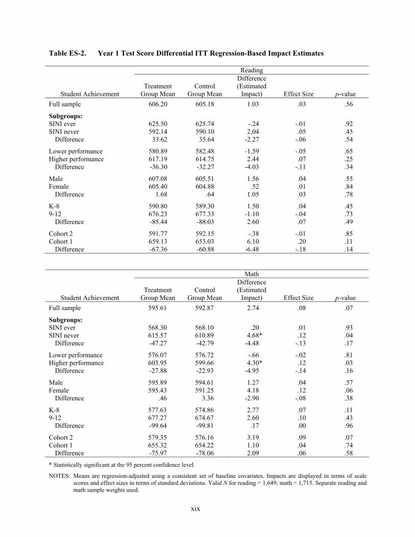
• The main models indicate that the Program generated no statistically significant impacts, positive or negative, on student reading or math achievement for the entire impact sample in year 1. One of the three alternative specifications indicated a positive and statistically significant math impact of 3.4 scale score points.
• No statistically significant achievement impacts were observed for the high-priority subgroup of students who had attended a SINI public school under NCLB before applying to the Program.
• The Program may have had an impact on math achievement for two subgroups of students with baseline characteristics associated with better academic preparation. The main models suggest that the OSP improved the math achievement of participating students who had not attended a SINI school by 4.7 scale score points and increased the math scores of those with relatively higher test score performance at baseline by 4.3 scale score points. However, these findings should be interpreted with caution, as adjustments for multiple comparisons suggested they may be false discoveries.
• No significant achievement impacts were observed for other subgroups of participating students, including those with lower test scores at baseline, girls, boys, elementary students, secondary students, or students within each of the individual cohorts that in combination made up the impact sample.
xix
Table ES-2. Year 1 Test Score Differential ITT Regression-Based Impact Estimates Reading
Student Achievement Treatment
Group Mean Control
Group Mean
Difference (Estimated
Impact) Effect Size p-value Full sample 606.20 605.18 1.03 .03 .56
Subgroups: SINI ever 625.50 625.74 -.24 -.01 .92 SINI never 592.14 590.10 2.04 .05 .45
Difference 33.62 35.64 -2.27 -.06 .54
Lower performance 580.89 582.48 -1.59 -.05 .65 Higher performance 617.19 614.75 2.44 .07 .25
Difference -36.30 -32.27 -4.03 -.11 .34
Male 607.08 605.51 1.56 .04 .55 Female 605.40 604.88 .52 .01 .84
Difference 1.68 .64 1.05 .03 .78
K-8 590.80 589.30 1.50 .04 .45 9-12 676.23 677.33 -1.10 -.04 .73
Difference -85.44 -88.03 2.60 .07 .49
Cohort 2 591.77 592.15 -.38 -.01 .85 Cohort 1 659.13 653.03 6.10 .20 .11
Difference -67.36 -60.88 -6.48 -.18 .14
Math
Student Achievement Treatment
Group Mean Control
Group Mean
Difference (Estimated
Impact) Effect Size p-value Full sample 595.61 592.87 2.74 .08 .07
Subgroups: SINI ever 568.30 568.10 .20 .01 .93 SINI never 615.57 610.89 4.68* .12 .04
Difference -47.27 -42.79 -4.48 -.13 .17
Lower performance 576.07 576.72 -.66 -.02 .81 Higher performance 603.95 599.66 4.30* .12 .03
Difference -27.88 -22.93 -4.95 -.14 .16
Male 595.89 594.61 1.27 .04 .57 Female 595.43 591.25 4.18 .12 .06
Difference .46 3.36 -2.90 -.08 .38
K-8 577.63 574.86 2.77 .07 .11 9-12 677.27 674.67 2.60 .10 .43
Difference -99.64 -99.81 .17 .00 .96
Cohort 2 579.35 576.16 3.19 .09 .07 Cohort 1 655.32 654.22 1.10 .04 .74
Difference -75.97 -78.06 2.09 .06 .58
* Statistically significant at the 95 percent confidence level.
NOTES: Means are regression-adjusted using a consistent set of baseline covariates. Impacts are displayed in terms of scale scores and effect sizes in terms of standard deviations. Valid N for reading = 1,649; math = 1,715. Separate reading and math sample weights used.
xx
• The Program had a substantial positive impact on parents’ views of school safety but not on students’ actual school experiences with dangerous activities. Parents in the treatment group perceived their child’s school to be less dangerous (an impact of –0.74 on a 10-point scale) than parents in the control group. Student reports of dangerous incidents in school did not differ systematically between the treatment and control groups.
• The Program also had an impact on parent satisfaction with their child’s school. For example, an additional 19 percent of the parents of students in the treatment group graded their child’s school “A” or “B” compared with the parents of control group students.
• For the most part, student satisfaction with their school was unaffected by the Program. The main exception was for students with lower test score performance at baseline, who on average assigned their schools significantly lower grades if they were in the treatment group.
Additional Findings Regarding Using a Scholarship and Attending a Private School (Non-experimental)
The results described above answer the question “what happened to OSP applicants who were offered a scholarship, whether or not a student used the scholarship to attend a private school?” Estimating the impact of using an OSP scholarship involves statistically adjusting the initial impact results to account for two groups of impact sample students: (1) the about 20 percent who received but failed to take up the scholarship offer, who presumably had zero impact from the Program, and (2) an estimated 4 percent in the control group who never received a scholarship offer but who, by virtue of having a sibling with an OSP scholarship, wound up in a participating private school (what we call “program-induced crossover”). These straightforward statistical adjustments yield what are typically called the “impact-on-the-treated” or IOT results. These adjustments increase the size of the scholarship offer effect estimate, but cannot make a statistically insignificant result significant. Therefore, the adjustments are only applied to results that were statistically significant at the scholarship offer stage of the analysis.
The statistically significant findings regarding the use of a scholarship include: • Using a scholarship led to positive impacts on math scores for students from non-SINI
schools (6.1 scale score points compared to 4.7 scale score points for the impact of scholarship award) and for students with higher test scores at baseline (5.6 scale score points compared to 4.3 scale score points for the impact of scholarship award). However, adjustments for multiple comparisons indicate both of these findings may be false discoveries.
xxi
• Scholarship use led to an average reduction of nearly a point on the 10-point danger perception index for parents, compared to a –0.74 point impact for the award of a scholarship.
• Using a scholarship significantly increased parent satisfaction with their child’s school. An additional 25 percent of the parents of scholarship users graded their child’s school “A” or “B” compared to the parents of control group students, while the difference was 19 percent for the impact of the offer of a scholarship.
Estimating the effect of attending a private school, regardless of whether an OSP scholarship was used, also begins with the original impact results but uses a more complex statistical procedure.6 Because this approach deviates somewhat from the overall experimental design of the evaluation, and yields estimates that are less precise, the private schooling results should be interpreted and used with caution. Like those applied to estimate the impact of OSP scholarship use, the private schooling adjustments increase the size of the scholarship offer effect estimate, but cannot make an insignificant result significant. Therefore, the procedure is only applied to results that were statistically significant at the scholarship offer stage of the analysis.
The main private schooling results suggest that • Private schooling was associated with higher math achievement for SINI-never
students (by 7.8 scale score points) and for students with higher test scores at baseline (by 6.7 scale score points), but both of these findings may be false discoveries due to multiple comparisons. These private schooling differences were larger than were the impacts of scholarship award and scholarship use for SINI-never students (4.7 points and 6.1 points, respectively) and for students with higher test scores at baseline (4.3 points and 5.6 points, respectively).
• Private schooling is associated with lower parent perceptions of danger and higher parent satisfaction. The average score for private school parents represented 1.14 fewer points or areas of concern on the 10-point school danger index than the average score for public school parents, compared to impacts of –0.74 points for scholarship award and a reduction of one point for scholarship use. Similarly, parents of private school students were 30 percent more likely to grade their child’s school an “A” or “B” than were parents of public school students, compared to impact on this measure of 19 percent for scholarship award and 25 percent for scholarship use.
6 The scholarship lottery is used as an instrumental variable (IV) to predict whether a student attended private school. Unlike an
indicator variable for actual attendance at a private school, the prediction of private school attendance using the scholarship lottery instrument is unbiased because it is the same for all treatment group students (and all control group students) regardless of their individual enrollment decisions.
xxii
These results can be placed in the context of other RCTs of scholarship programs for low-income students, which suggest no consistent pattern of academic achievement impacts for the first year of program participation. Among such evaluations of four privately funded scholarship programs, one study of the Charlotte, North Carolina, program clearly found statistically significant overall impacts on math and reading for the first year, while one of three analyses of the New York City program found overall impacts on math achievement (Barnard, Frangakis, Hill, and Rubin, 2003; Greene 2000). When African-Americans are considered separately, a group that makes up nearly 90 percent of the OSP impact study sample, two of three analyses of the New York City program suggest there were achievement gains in math for African-American students in some grade levels (Mayer, Peterson, Myers, Tuttle, and Howell, 2002), but studies of the Dayton, Ohio, and earlier District of Columbia programs found no impacts for this group until students were in the program for 2 years (Howell, Wolf, Campbell, and Peterson, 2002). In contrast, all of the randomized controlled trials that measured parent satisfaction and perceptions of school safety found positive impacts similar to those demonstrated by the OSP the first year (Greene, 2000; Howell and Peterson et al., 2002).
The findings here are based on information collected only a year after students applied to the
Program and may not reflect the consistent impacts of the OSP over a longer period of time. Families that apply to voucher programs intend for their children to leave their current public schools and, in the case of the OSP, a much higher share of students in the treatment group (91.3 percent) switched schools—mostly from public to private—compared to those in the control group (56.6 percent). The first-year results, therefore, provide an early look at student experiences in what was a transitional year for most of them. Future reports will examine impacts 2 and 3 years after application to the Program, when any short-term effect of students’ transition to new schools may have dissipated. The later reports will also consider additional outcome measures, assess the extent to which school characteristics are associated with impacts, and examine how the DC public school system is changing in response to the Program.

1
1. Introduction
School choice remains an important part of the national discussion on education reform strategies and their benefits. While a variety of policies encourage parents’ selection of schools for their children―for example, charter schools, magnet schools, and district open enrollment―scholarships that allow students to attend a private school have received the most attention. The U.S. Congress’ passage of the District of Columbia School Choice Incentive Act of 20031 in January 2004 provided a unique opportunity not only to implement a system of private school choice for low-income students in the District, but also to rigorously assess the effects of the Program on students, parents, and the existing school system. This report describes the first-year impacts of the Program on those who applied for and were given the option to move from a public school to a participating private school of their choice.
1.1 The DC Opportunity Scholarship Program
The 2004 statute established what is now called the DC Opportunity Scholarship Program (OSP)—the first Federal government initiative to provide K-12 education scholarships to families to send their children to private schools. The OSP has the following programmatic elements:
• To be eligible, students entering grades K-12 must reside in the District and have a
family income at or below 185 percent of the Federal poverty line.
• Participating students receive scholarships of up to $7,500 to cover the costs of tuition, school fees, and transportation to a participating private school.
• Scholarships are renewable for up to 5 years (as funds are appropriated), so long as students remain eligible for the Program and remain in good academic standing at the private school they are attending.
• In a given year, if there are more eligible applicants than available scholarships or open slots in private schools, applicants are to be awarded scholarships by random selection (e.g., by lottery).
• In making scholarship awards, priority is given to students attending public schools designated as in need of improvement (SINI) under the No Child Left Behind (NCLB) Act and to families that lack the resources to take advantage of school choice options.
1 Title III of Division C of the Consolidated Appropriations Act, 2004, P.L. 108-199.
2
• Private schools participating in the Program must be located in the District of Columbia and must agree to requirements regarding nondiscrimination in admissions, fiscal accountability, and cooperation with the evaluation.
Following passage of the legislation, the Washington Scholarship Fund (WSF), a 501(c)3 organization in the District of Columbia, was selected in late March 2004 by the U.S. Department of Education (ED) to implement the OSP, under the supervision of both ED’s Office of Innovation and Improvement and the Office of the Mayor of the District of Columbia. Since then, the WSF has worked with its implementation partners2 to finalize the Program design, establish protocols, recruit applicants and schools, award scholarships, and place and monitor scholarship awardees in participating private schools. The funds appropriated for the OSP are sufficient to support approximately 1,700 to 1,800 students in a given year, depending on the cost of the participating private schools that they attend.
To date, there have been three rounds of applicants to the OSP: • Applicants in spring 2004 (cohort 1),
• Applicants in spring 2005 (cohort 2), and
• Applicants in spring 2006 (cohort 3).
This report, and the mandated evaluation (see below), focuses on a subset of applicants in spring 2004 and in spring 2005 (cohorts 1 and 2). In these 2 years, there were a total of 5,818 applicants, of which 4,047 were deemed eligible to participate in the Program. Scholarships were offered to 2,454 of these eligible applicants, and 1,824 students used their scholarship in the first year of scholarship receipt (table 1-1). Descriptive reports on each of these first 2 years of Program implementation have been previously prepared and released (Wolf et al., 2005; Wolf et al., 2006).3 A much smaller number of cohort
2 The WSF has joined with Capital Partners for Education, DC Parents for School Choice, and Fight for Children—all District-
based nonprofit organizations, to assist in client recruitment and implementation activities. 3 Both of these reports are available on the Institute of Education Sciences’ Web site at: http://www.ies.ed.gov/ncee.
3
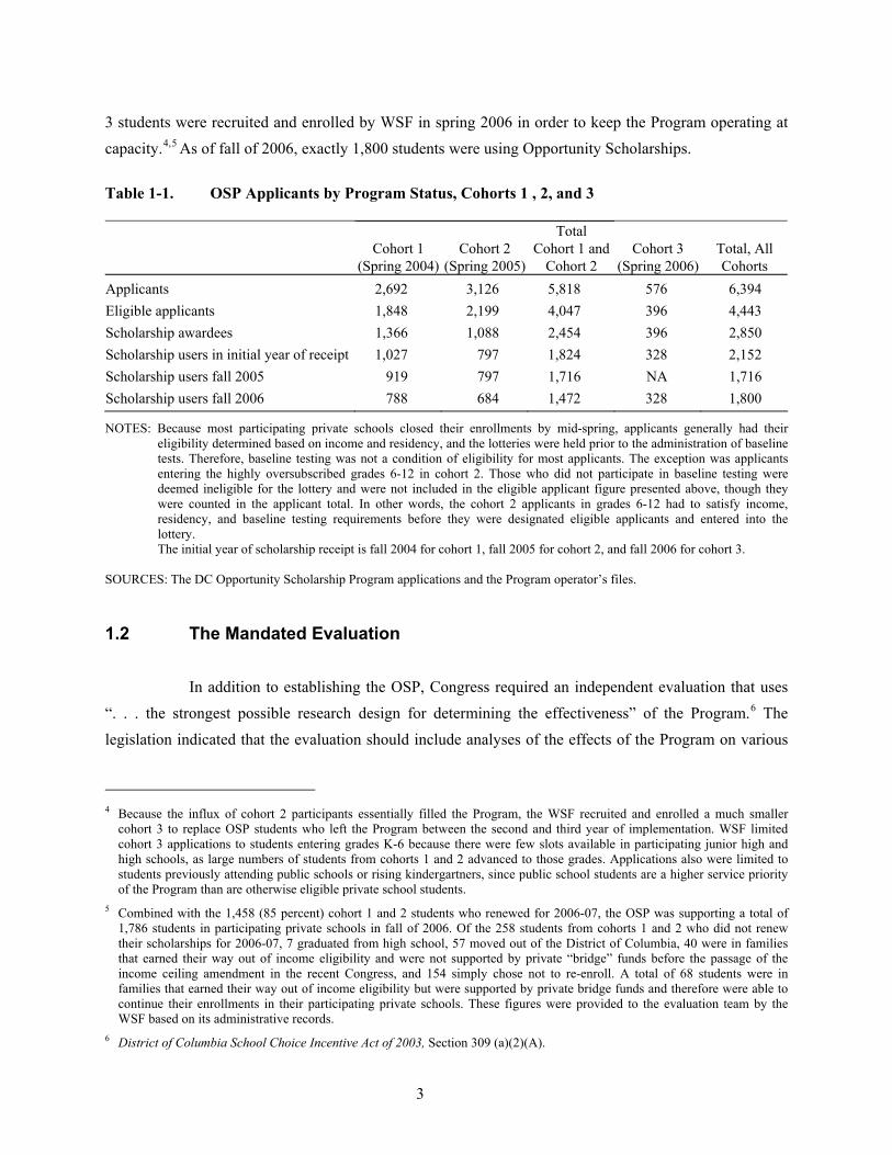
3 students were recruited and enrolled by WSF in spring 2006 in order to keep the Program operating at capacity.4,5 As of fall of 2006, exactly 1,800 students were using Opportunity Scholarships. Table 1-1. OSP Applicants by Program Status, Cohorts 1 , 2, and 3
Cohort 1 (Spring 2004)
Cohort 2 (Spring 2005)
Total Cohort 1 and
Cohort 2 Cohort 3
(Spring 2006) Total, All Cohorts
Applicants 2,692 3,126 5,818 576 6,394 Eligible applicants 1,848 2,199 4,047 396 4,443 Scholarship awardees 1,366 1,088 2,454 396 2,850 Scholarship users in initial year of receipt 1,027 797 1,824 328 2,152 Scholarship users fall 2005 919 797 1,716 NA 1,716 Scholarship users fall 2006 788 684 1,472 328 1,800
NOTES: Because most participating private schools closed their enrollments by mid-spring, applicants generally had their eligibility determined based on income and residency, and the lotteries were held prior to the administration of baseline tests. Therefore, baseline testing was not a condition of eligibility for most applicants. The exception was applicants entering the highly oversubscribed grades 6-12 in cohort 2. Those who did not participate in baseline testing were deemed ineligible for the lottery and were not included in the eligible applicant figure presented above, though they were counted in the applicant total. In other words, the cohort 2 applicants in grades 6-12 had to satisfy income, residency, and baseline testing requirements before they were designated eligible applicants and entered into the lottery. The initial year of scholarship receipt is fall 2004 for cohort 1, fall 2005 for cohort 2, and fall 2006 for cohort 3.
SOURCES: The DC Opportunity Scholarship Program applications and the Program operator’s files.
1.2 The Mandated Evaluation
In addition to establishing the OSP, Congress required an independent evaluation that uses “. . . the strongest possible research design for determining the effectiveness” of the Program.6 The legislation indicated that the evaluation should include analyses of the effects of the Program on various
4 Because the influx of cohort 2 participants essentially filled the Program, the WSF recruited and enrolled a much smaller
cohort 3 to replace OSP students who left the Program between the second and third year of implementation. WSF limited cohort 3 applications to students entering grades K-6 because there were few slots available in participating junior high and high schools, as large numbers of students from cohorts 1 and 2 advanced to those grades. Applications also were limited to students previously attending public schools or rising kindergartners, since public school students are a higher service priority of the Program than are otherwise eligible private school students.
5 Combined with the 1,458 (85 percent) cohort 1 and 2 students who renewed for 2006-07, the OSP was supporting a total of 1,786 students in participating private schools in fall of 2006. Of the 258 students from cohorts 1 and 2 who did not renew their scholarships for 2006-07, 7 graduated from high school, 57 moved out of the District of Columbia, 40 were in families that earned their way out of income eligibility and were not supported by private “bridge” funds before the passage of the income ceiling amendment in the recent Congress, and 154 simply chose not to re-enroll. A total of 68 students were in families that earned their way out of income eligibility but were supported by private bridge funds and therefore were able to continue their enrollments in their participating private schools. These figures were provided to the evaluation team by the WSF based on its administrative records.
6 District of Columbia School Choice Incentive Act of 2003, Section 309 (a)(2)(A).
4
academic and non-academic outcomes of concern to policymakers.7 This legislative mandate led the evaluators to focus on the following research questions:
1. What is the impact of the Program on student academic achievement? Does the award
of a scholarship improve a student’s academic achievement in the core subjects of reading and mathematics?
2. What is the impact of the Program on other student measures (e.g., school attendance and educational attainment)? Does the award of a scholarship improve other important aspects of a student’s education that are related to school success?
3. What effect does the Program have on school safety and satisfaction? Does the award of a scholarship increase student and/or parent perceptions of safety with school? Does the award of a scholarship increase student and/or parent satisfaction with school?
4. What is the effect of attending private versus public schools? Because some students offered scholarships will choose not to use them, and some members of the control group will attend private schools, the study will also examine the results associated with private school attendance with or without a scholarship.8
5. To what extent is the Program influencing public schools and expanding choice options for parents in Washington, DC? That is, to what extent has the scholarship program had a broader effect on public and private schools in the City, such as instructional changes by public schools to respond to the new competition from private schools.
ED’s Institute of Education Sciences (IES), responsible for the mandated evaluation, determined that the foundation of the evaluation would be a randomized controlled trial (RCT), comparing outcomes of eligible applicants (students and their parents) randomly assigned to receive or not receive a scholarship. This decision was based on the mandate to use rigorous evaluation methods, the expectation that there would be more applicants than funds and private school spaces available, and the Program requirement to use lotteries to determine who receives a scholarship when there is more demand for scholarships than can be accommodated. The law clearly specified that such a comparison in
7 “The issues to be evaluated include the following: (A) A comparison of the academic achievement of participating eligible
students…to the achievement of…the eligible students in the same grades…who sought to participate in the scholarship program but were not selected. (B) The success of the programs in expanding choice options for parents. (C) The reasons parents choose for their children to participate in the programs. (D) A comparison of retention rates, dropout rates, and (if appropriate) graduation and college admission rates… (E) The impact of the program on students, and public elementary schools and secondary schools, in the District of Columbia. (F) A comparison of the safety of the schools attended by students who participate in the programs and the schools attended by students who do not participate in the programs. (G) Such other issues as the Secretary considers appropriate for inclusion in the evaluation.” (Section 309 (4)). The statute also says that, “(A) the academic achievement of students participating in the program; (B) the graduation and college admission rates of students who participate in the program, where appropriate; and (C) parental satisfaction with the program” should be examined in the reports delivered to the Congress. (Section 310 (b)(1)).
8 Although the statute does not explicitly request analyses of the effects of private schooling, it does request comparisons between “program participants,” which could be understood to mean students using a scholarship to attend private school, and non-participants.
5
outcomes be made.9 An RCT design is widely viewed as the best method for identifying the independent effect of programs on subsequent outcomes and has been used by researchers conducting impact evaluations of other scholarship programs in New York City; Dayton, Ohio; and Washington, DC.10
1.3 Contents of This Report
This report is the third in a series of required annual evaluation reports to Congress. It presents the impacts of the Program on students and families 1 year after they applied and had the chance of being awarded and using a scholarship to attend a participating private school.
In presenting these impacts, we first provide some background on the implementation of the
OSP and the students and schools that are part of the Program, much of which has been described in prior evaluation reports (chapter 2). We then present the research and analysis methods used in the impact evaluation, including data collection, imputation, statistical weighting, and the models used to estimate Program impacts (chapter 3). The main impact results, both for the overall group and for important subgroups of applicants, are described in chapter 4; these findings address whether students who received a scholarship through the lotteries (and their parents) benefited from 1 year in the Program by comparing their early outcomes to the outcomes of students who applied for but did not receive scholarships through the lotteries. The final chapter (chapter 5) deviates somewhat from the random assignment design to assess the impact of the OSP on those students who actually used their scholarship to attend a private school, since not all scholarship awardees did, and to estimate differences in outcomes between those who attended private schools and those who did not, using the lottery results as an instrument to control for likely selectivity in such non-random participant samples.
The findings here are based on information collected only a year after students applied to the
Program and may not reflect the consistent impacts of the OSP over a longer period of time. Families that apply to voucher programs intend for their children to leave their current public schools, and, in the case
9 See Section 309 (a)(4)(A)(ii). 10 RCTs are commonly referred to as the “gold standard” for evaluating educational interventions; when mere chance determines
which eligible applicants receive access to school choice, the students who apply but are not admitted make up an ideal “control group” for comparison with the school choice “treatment group.” Both groups of participants are equally motivated to obtain new educational options, and nothing except a random draw distinguishes those who receive the opportunity from those who do not. Therefore, any differences in the two groups in subsequent years can be attributed to the impact of the program. In contrast, the results of school choice studies that are not based on RCTs must be interpreted and used more cautiously because comparisons between the applicants and a group of students who chose not to apply will likely reflect not only the impact of the program but also initial differences between the groups in motivation and other unmeasured characteristics. See chapter 3 for more detail on the RCT design and analysis.
6
of the OSP, a much higher share of students in the treatment group (91.3 percent) switched schools—mostly from public to private—compared to those in the control group (56.6 percent). The first-year results, therefore, provide an early look at student experiences in what was a transitional year for most of them. Future reports will examine impacts 2 and 3 years after application to the Program, when any short-term effect of students’ transition to new schools may have dissipated. The later reports will also consider additional outcome measures, assess the extent to which school characteristics are associated with impacts, and examine how the DC public school system is changing in response to the Program.
In the end, the findings in this and subsequent reports are a reflection of the particular
Program elements that evolved from the law passed by Congress and the characteristics of the students, families, and schools―both public and private―that exist in the Nation’s capital. The same program implemented in another city might yield different results, and a different scholarship program administered in Washington, DC, might also produce different outcomes. Thus, while the results presented here will contribute to the research evidence on scholarships in general, they are most relevant to the specific program that is being evaluated and described in the following chapters.
7
2. Early Implementation of the Program and the Sample for the Impact Analysis
The recruitment, application, and lottery process conducted under the guidance of the Washington Scholarship Fund (WSF) created the foundation for the impact analysis that is the focus of this report. The schools recruited into the Opportunity Scholarship Program (OSP) determined the number of private school slots available and, ultimately, the quality of instruction to which Program participants were exposed. The students who applied, combined with the slots available, established the parameters for the lotteries and may well influence whether they benefit from the Program. This chapter provides additional detail regarding the OSP, including the design of the lotteries that enable the study to be experimental in design and execution, the characteristics of the students that are the Program and impact study participants, and the types of schools the students were enrolled in when they applied and 1 year later. It is designed to communicate how and when the Program was implemented and the conditions under which the impact evaluation took place.
2.1 Student Recruitment
Very quickly after it received the grant to operate the OSP, WSF and its partners began to recruit families to participate in the Program. In addition to numerous mailings and visits to schools and churches, application events were held throughout the District of Columbia. The form necessary for applying to the Program required parents to confirm that student applicants met all eligibility criteria―residing in DC and entering kindergarten through grade 12―and to provide documentation for verification purposes, including residency and income; it also functioned as the baseline or “pre-program” survey for the evaluation and included a parent consent form for the evaluation’s data collection.
Over the first 2 years of recruitment, in spring 2004 and 2005, WSF received applications
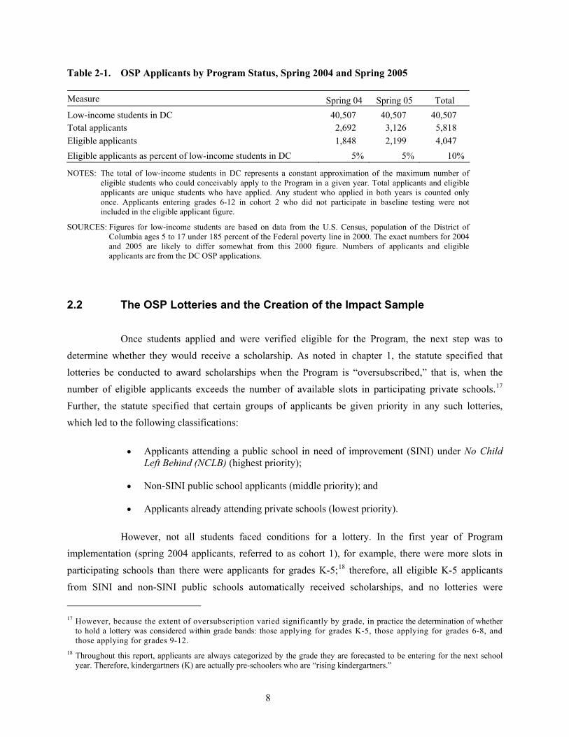
from 5,818 students. Of these, approximately 70 percent (4,047 of 5,818) were eligible to enter the Program. These eligible applicants represent about 10 percent of the population in Washington, DC, that met the Program’s eligibility criteria, according to 2000 Census figures (table 2-1).
8
Table 2-1. OSP Applicants by Program Status, Spring 2004 and Spring 2005 Measure Spring 04 Spring 05 Total Low-income students in DC 40,507 40,507 40,507 Total applicants 2,692 3,126 5,818 Eligible applicants 1,848 2,199 4,047 Eligible applicants as percent of low-income students in DC 5% 5% 10%
NOTES: The total of low-income students in DC represents a constant approximation of the maximum number of eligible students who could conceivably apply to the Program in a given year. Total applicants and eligible applicants are unique students who have applied. Any student who applied in both years is counted only once. Applicants entering grades 6-12 in cohort 2 who did not participate in baseline testing were not included in the eligible applicant figure.
SOURCES: Figures for low-income students are based on data from the U.S. Census, population of the District of Columbia ages 5 to 17 under 185 percent of the Federal poverty line in 2000. The exact numbers for 2004 and 2005 are likely to differ somewhat from this 2000 figure. Numbers of applicants and eligible applicants are from the DC OSP applications.
2.2 The OSP Lotteries and the Creation of the Impact Sample
Once students applied and were verified eligible for the Program, the next step was to determine whether they would receive a scholarship. As noted in chapter 1, the statute specified that lotteries be conducted to award scholarships when the Program is “oversubscribed,” that is, when the number of eligible applicants exceeds the number of available slots in participating private schools.17 Further, the statute specified that certain groups of applicants be given priority in any such lotteries, which led to the following classifications:
• Applicants attending a public school in need of improvement (SINI) under No Child
Left Behind (NCLB) (highest priority);
• Non-SINI public school applicants (middle priority); and
• Applicants already attending private schools (lowest priority).
However, not all students faced conditions for a lottery. In the first year of Program implementation (spring 2004 applicants, referred to as cohort 1), for example, there were more slots in participating schools than there were applicants for grades K-5;18 therefore, all eligible K-5 applicants from SINI and non-SINI public schools automatically received scholarships, and no lotteries were
17 However, because the extent of oversubscription varied significantly by grade, in practice the determination of whether
to hold a lottery was considered within grade bands: those applying for grades K-5, those applying for grades 6-8, and those applying for grades 9-12.
18 Throughout this report, applicants are always categorized by the grade they are forecasted to be entering for the next school year. Therefore, kindergartners (K) are actually pre-schoolers who are “rising kindergartners.”

9
conducted at that level. In contrast, there were more eligible public school applicants in cohort 2 (spring 2005) than there were available slots at all grades levels, so that all of those applicants were subject to a lottery to determine scholarship awards. One other difference is that, because there were sufficient funds available in school year 2004-05, applicants seeking an OSP scholarship but who were already attending a private school were entered into a lottery the first year. In cohort 2, there was sufficient demand from public school applicants that lotteries were conducted only for them; applicants who were already attending a private school (the lowest priority group) were not entered into a lottery and did not receive scholarships.
Lottery Design and Outcomes
In general, the probability of being awarded a scholarship through a lottery was based on a given student’s priority status and the ratio of slots to applicants in that student’s grade band (grades K-5, grades 6-8, and grades 9-12). Within a given grade band, applicants from SINI-designated public schools were assigned award probabilities approximately one-third higher than those from non-SINI public schools. Eligible applicants from private schools were assigned much lower probabilities than either type of public school applicants in the first year, and an award probability of 0 in the second year, when the Program was oversubscribed with higher priority public school applicants. Across the grade bands, the award probabilities were determined by the degree of oversubscription for those grades. Given the likelihood that some students would choose not to use the scholarships that were awarded to them, based on previous scholarship program experiments, award probabilities were then adjusted to “over-award” scholarships by approximately 20 percent19 (see Howell and Peterson et al., 2002, p. 44).
In total, after the first 2 years of Program implementation, the WSF had awarded
Opportunity Scholarships to 2,454 students. The total awards to the three priority subgroups were • 508 scholarship awards to public school students attending schools designated as SINI
the year before they entered the lottery;
• 1,730 scholarship awards to students in non-SINI public schools; and
• 216 scholarship awards to students attending private schools but otherwise eligible for the Program (in the first year only).
19 For example, the proportion of awarded scholarships that were actually used in the first year of the previous experiments in
Washington, DC; Dayton, Ohio; and New York City ranged from 68 to 82 percent.

10
The timing of the release of annual SINI designations complicated the task of assigning SINI applicants priority in the lotteries. To enable students who were offered scholarships to obtain a placement in a participating private school, scholarships had to be awarded in April-June of each implementation year. However, the list of District of Columbia public schools designated as in need of improvement each year was not released until August. Therefore, priority designations for the lotteries had to be based on the shorter list of schools designated SINI during the year prior to the lottery. About 40 percent of applicants were from schools designated SINI for the year the students would be leaving those schools to participate in the OSP. For cohort 1, 37 percent were SINI, and for cohort 2, just under 43 percent were SINI. In total, 44 percent of OSP applicants were from schools designated as SINI between 2003 and 2005, a period when the number of SINI schools in the District jumped from 15 to 101 (table 2-2).
Table 2-2. Percent of Public School Applicants From SINI Schools, Spring 2004 and Spring 2005 Timing of SINI Designation Total Spring 2004 Spring 2005 SINI in fall 2003 (N=15) 4.9 5.9 4.2 SINI in fall 2004 (N=90) 36.9 37.1 36.7 SINI in fall 2005 (N=101) 43.7 44.8 42.8 All eligible public school applicants 3,159 1,343 1,816
NOTE: The figures in bold are those most relevant for each cohort.
SOURCES: The DC Opportunity Scholarship Program applications and the District of Columbia Public Schools Web site.
Creation of the Impact Sample
The impact sample is a direct result of the lotteries and the critical component of the legislatively required rigorous evaluation of the OSP. Impact evaluations compare the outcomes for a group of applicants or study participants, all of whom were randomly awarded to either receive access to the intervention (e.g., an OSP scholarship) or to not receive access. The lotteries conducted for some of the OSP applicants in years 1 and 2 satisfy these requirements. Since the intervention under consideration is an Opportunity Scholarship to attend a private school, the impact analysis focuses on the population of applicants for whom private schooling represented a new opportunity. Thus, the impact sample for this evaluation comprised all eligible applicants who were previously attending public schools (or were rising kindergartners) AND were subject to a lottery to determine whether they would receive an Opportunity Scholarship (figure 2-1, shaded area).

11
Figure 2-1. Construction of the Impact Sample From the Applicant Pool, Cohorts 1 and 2
All eligible applicants
C1=1,848C2=2,199
Total=4,047
PublicC1=1,343C2=1,816
Total=3,159
PrivateC1=505C2=383
Total=888
Randomized(impact sample)
C1=492C2=1,816
Total=2,308
ScholarshipC1=216
C2=0Total=216
Non-ScholarshipC1=289C2=383
Total=672
Non-Scholarship(control)C1=193C2=728
Total=921
NOTES: C1 = Cohort 1 (applicants in spring 2004) C2 = Cohort 2 (applicants in spring 2005) Total = C1 and C2
Randomized (non-impact)
C1=505C2=0
Total=505
Non-Randomized(non-impact)
C1=851C2=0
Total=851
Scholarship(treatment)
C1=299C2=1,088
Total=1,387
a Non-Randomized(non-impact)
C1=0C2=383
Total=383
a
ScholarshipC1=851
C2=0Total=851
aThe group of applicants who were not randomly assigned includes: in cohort 1, public school applicants from SINI schools or who were entering grades K-5 (all received a scholarship), and in cohort 2, private school applicants, the lowest priority group (none received a scholarship because it was clear the Program would be filled with higher priority public school applicants).
The total pool of eligible applicants comprised 1,848 applicants in cohort 1 (spring 2004)
and 2,199 applicants in cohort 2 (spring 2005). Of those eligible applicants, 492 in cohort 1 and 1,816 in cohort 2 met the criteria to be randomly assigned by lottery to the treatment and control groups. In cohort 1, a total of 299 students were randomized into the treatment condition and 193 into the control condition. In cohort 2, some 1,088 students were randomized into the treatment condition and 728 into the control

12
condition. The impact sample comprised by these groups totals 2,308 students:20 1,387 students in the treatment condition and 921 in the control condition. The more than 2,300 students in the impact sample is a large group relative to the impact samples used in other evaluations of private school scholarship programs (803 to 1,960 students) (Howell and Peterson et al., 2002, p. 44).
2.3 Characteristics of the Impact Sample
The OSP impact sample group, 57 percent of eligible applicants, will provide the most reliable evidence regarding whether and how the OSP has influenced the educational experiences and outcomes of scholarship awardees.21 The characteristics of this group are a factor in determining whether the random assignment was completed properly and possibly the extent of Program impacts.
Overall Sample
The students in the impact sample as a whole reflect the Program’s income eligibility criteria and priorities as specified in the authorizing legislation (table 2-3, second column):
20 A total of five members of the cohort 1 control group were awarded scholarships by lottery in the summer of 2005 and a total
of six members of the control group (cohorts 1 and 2) were awarded scholarships by lottery in the summer of 2006 as part of the control group follow-up lottery to reward control group members who cooperate with the evaluation’s testing requirements. Control group students who win a follow-up incentive lottery are included in the analysis until they have been offered a scholarship, at which point they are excluded from subsequent data collection activities because their initial random assignment has been deliberately undermined. The exclusion of the 11 control group lottery winners did not affect the size of the control group sample for this report, as they all provided 1-year outcome data before being awarded their scholarships; however, the control group population for all future impact studies will not include those 11 students.
21 The subgroups of eligible applicants to the Program who did not fit the criteria for the impact sample include eligible applicants in cohorts 1 and 2 who were already attending private schools (n=888) and two groups of public school applicants in cohort 1 who were automatically awarded scholarships (n=851), specifically those from SINI public schools because of their high service priority and those applying from grades K-5 because there were sufficient private school slots in those grades to accommodate all of those applicants that year. The exclusion of these non-randomized subgroups from the impact evaluation has implications for the ability to generalize the study results. Since the experiences of students who sought and obtained a scholarship presumably to continue their private schooling will likely differ from public school applicants who are the subject of this experimental study, readers are cautioned not to generalize the results of this impact study to existing private school populations. In addition, the cohort 1 K-5 population that automatically received scholarships because their grade levels were not oversubscribed differ in important ways from the cohort 2 K-5 population that was randomized into the impact study. At baseline, the cohort 1 K-5 group was somewhat older, more likely to be from a SINI-ever school, African American, and have a special educational need, and had higher baseline test scores and family income than cohort 2 K-5 participants, who were more likely to be Hispanic (see appendix A). The cohort 1 applicants from SINI-designated schools numbered only 79. The 655 cohort 2 applicants from SINI-designated schools provide a great deal of information about the impact of the Program on SINI participants. Despite the differences in the population of program participants inside and outside of the evaluation described above, the impact sample still retains characteristics of economic and social disadvantage that are common to urban families targeted for participation by school choice programs.
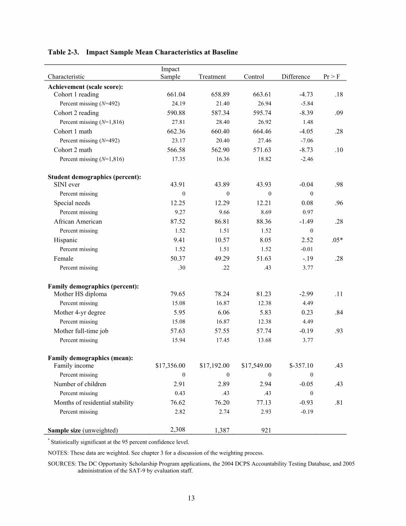
13
Table 2-3. Impact Sample Mean Characteristics at Baseline
Characteristic Impact Sample Treatment Control Difference Pr > F
Achievement (scale score): Cohort 1 reading 661.04 658.89 663.61 -4.73 .18
Percent missing (N=492) 24.19 21.40 26.94 -5.84 Cohort 2 reading 590.88 587.34 595.74 -8.39 .09
Percent missing (N=1,816) 27.81 28.40 26.92 1.48 Cohort 1 math 662.36 660.40 664.46 -4.05 .28
Percent missing (N=492) 23.17 20.40 27.46 -7.06 Cohort 2 math 566.58 562.90 571.63 -8.73 .10
Percent missing (N=1,816) 17.35 16.36 18.82 -2.46 Student demographics (percent):
SINI ever 43.91 43.89 43.93 -0.04 .98 Percent missing 0 0 0 0
Special needs 12.25 12.29 12.21 0.08 .96 Percent missing 9.27 9.66 8.69 0.97
African American 87.52 86.81 88.36 -1.49 .28 Percent missing 1.52 1.51 1.52 0
Hispanic 9.41 10.57 8.05 2.52 .05* Percent missing 1.52 1.51 1.52 -0.01
Female 50.37 49.29 51.63 -.19 .28 Percent missing .30 .22 .43 3.77
Family demographics (percent):
Mother HS diploma 79.65 78.24 81.23 -2.99 .11 Percent missing 15.08 16.87 12.38 4.49
Mother 4-yr degree 5.95 6.06 5.83 0.23 .84 Percent missing 15.08 16.87 12.38 4.49
Mother full-time job 57.63 57.55 57.74 -0.19 .93 Percent missing 15.94 17.45 13.68 3.77
Family demographics (mean):
Family income $17,356.00 $17,192.00 $17,549.00 $-357.10 .43 Percent missing 0 0 0 0
Number of children 2.91 2.89 2.94 -0.05 .43 Percent missing 0.43 .43 .43 0
Months of residential stability 76.62 76.20 77.13 -0.93 .81 Percent missing 2.82 2.74 2.93 -0.19
Sample size (unweighted) 2,308 1,387 921 * Statistically significant at the 95 percent confidence level.
NOTES: These data are weighted. See chapter 3 for a discussion of the weighting process.
SOURCES: The DC Opportunity Scholarship Program applications, the 2004 DCPS Accountability Testing Database, and 2005 administration of the SAT-9 by evaluation staff.
14
• The average impact sample student at the time of application had a reading scale score of 608 and a math scale score of 588, which equate to the 33rd National Percentile Rank (NPR) in reading and the 31st NPR in math.22
• About 44 percent of the impact sample was attending public schools designated SINI between 2003 and 2005.
• Twelve percent were described by their parents as having special needs.
• Nearly 90 percent were identified by their parents as African American, and 9 percent were identified as being of Hispanic ethnicity.
• They are evenly divided between males and females.
• Although 80 percent of their mothers reported having a high school diploma, only 6 percent said they had a bachelor’s degree; 58 percent of the mothers reported working full time.
• Their average household at the time of application had almost three children supported by an annual income of $17,356.
Treatment vs. Control Groups
An important strength of experimental methods of analysis is that the assignment of study participants to the treatment and control groups creates two analytic groups that are, on average, statistically similar at the time of random assignment.23 The treatment, in this case the offer of an Opportunity Scholarship, is provided to one group, and any subsequent differences in outcomes observed between the two groups can be ascribed to the impact of that treatment.
To see how the random assignment process works, we compare the characteristics of the
treatment and control groups as measured at baseline—prior to the Program intervention. The subgroup of students in the impact sample randomly assigned to the treatment group (table 2-3, treatment group column) is statistically similar to the randomized control group (table 2-3, control group column) in all but one instance.24 This pattern of characteristics across the treatment and control components of the overall impact sample is consistent with what we would expect from scholarship lotteries designed to
22 The average NPRs for the impact sample were computed by taking the weighted average NPRs within the various grades using
pre-imputation baseline test scores. 23 Randomized groups are not necessarily identical; however, when they do occasionally differ significantly regarding a certain
characteristic, the difference is due to chance and not because of the decisions or behaviors of study participants. 24 The one exception was Hispanic ethnicity, as the treatment group has a higher proportion of members who self-identify as
Hispanic than does the control group. Statistical theory predicts that 1 significant difference out of 16 in group characteristics is what would be expected by chance.

15
generate a representative treatment group of scholarship awardees and a statistically similar comparison group of control students.25
2.4 Schools Attended by OSP Applicants
Nearly two-thirds of District private schools have agreed to participate in the OSP. • 58 (53 percent) of the 109 private elementary and secondary schools in DC in 2004
agreed to participate in the Program in the first year of implementation.
• 68 (65 percent) of the 104 District private schools in 2005, including all the schools that participated in the first year, chose to participate in the OSP during the second year of implementation.
• Of the 68 participating schools in fall 2005, 60 (88 percent) had OSP students enrolled at that time.
• Members of the impact sample were attending 47 (69 percent) of the 68 participating schools 1 year after being awarded their scholarships.
Characteristics of All Participating Schools
The private schools participating in the OSP represent the choice set presented to parents whose children received scholarships. As such, the features of these schools, whether or not any OSP students enrolled in them, are relevant to a description of the OSP as a school choice program.
The religious status and affiliation of the participating schools varies (figure 2-2): of the 68
private schools participating in the Program in 2005-06, 23 (34 percent) were schools of the Catholic Archdiocese of Washington, 15 (22 percent) were non-Catholic faith-based schools, 16 (24 percent) were members of the Association of Independent Schools of Greater Washington (AISGW), and 14 (21 percent) were independent private schools that were neither faith-based nor members of the AISGW.26 25 Since factors such as attendance at a SINI-designated school and grade band affected each student’s probability of being
awarded a scholarship, these calculations of subgroup averages are based on observations that have been weighted to eliminate any compositional differences induced by the differential treatment probabilities within priority and grade band strata. Additional detail regarding the weighting procedures is provided in the next chapter.
26 Many members of the AISGW have religious names and traditions; however, they all operate independently of any direct influence by the authorities of a particular sectarian religion. Therefore, they have been classified as a particular category of school, neither fully faith-based nor fully non-faith based. These figures differ slightly from those originally presented in the first- and second-year descriptive reports on the Program, since those reports used a less differentiated classification scheme of Catholic, non-Catholic religious, secular, and unknown.
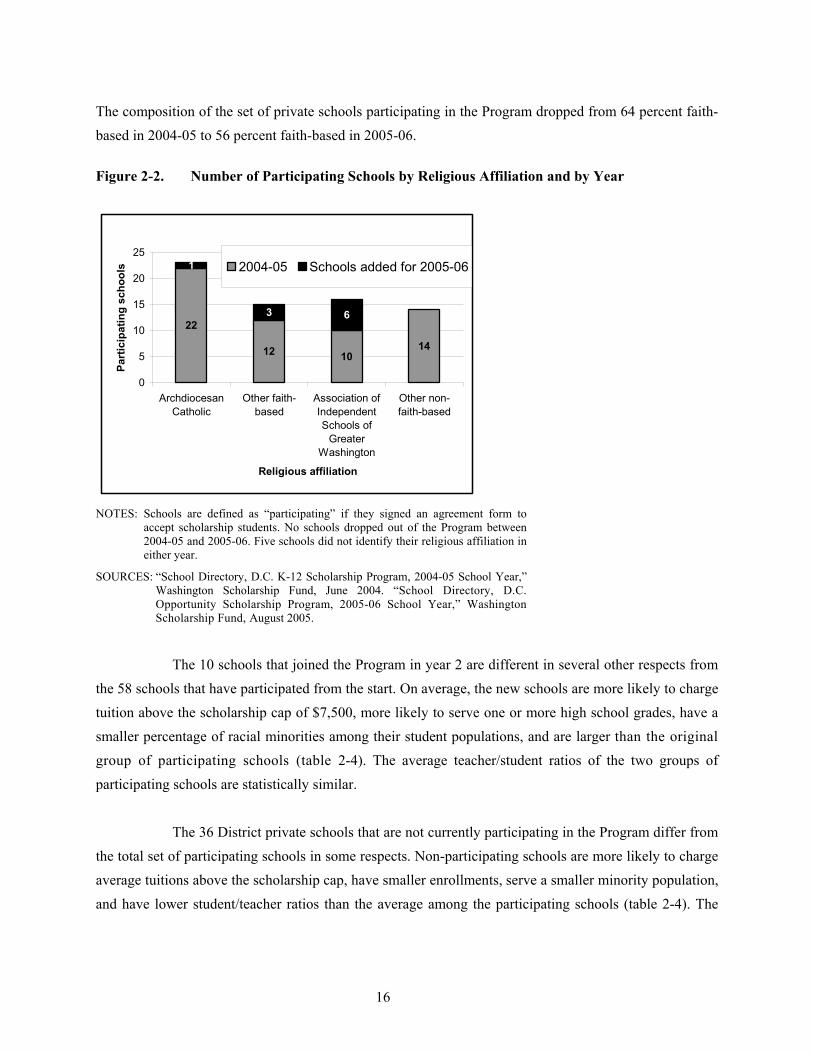
16
The composition of the set of private schools participating in the Program dropped from 64 percent faith-based in 2004-05 to 56 percent faith-based in 2005-06.
Figure 2-2. Number of Participating Schools by Religious Affiliation and by Year
22
12 1014
1
3 6
0
5
10
15
20
25
ArchdiocesanCatholic
Other faith-based
Association ofIndependentSchools of
GreaterWashington
Other non-faith-based
Religious affiliation
Part
icip
atin
g sc
hool
s 2004-05 Schools added for 2005-06
NOTES: Schools are defined as “participating” if they signed an agreement form to
accept scholarship students. No schools dropped out of the Program between 2004-05 and 2005-06. Five schools did not identify their religious affiliation in either year.
SOURCES: “School Directory, D.C. K-12 Scholarship Program, 2004-05 School Year,” Washington Scholarship Fund, June 2004. “School Directory, D.C. Opportunity Scholarship Program, 2005-06 School Year,” Washington Scholarship Fund, August 2005.
The 10 schools that joined the Program in year 2 are different in several other respects from
the 58 schools that have participated from the start. On average, the new schools are more likely to charge tuition above the scholarship cap of $7,500, more likely to serve one or more high school grades, have a smaller percentage of racial minorities among their student populations, and are larger than the original group of participating schools (table 2-4). The average teacher/student ratios of the two groups of participating schools are statistically similar.
The 36 District private schools that are not currently participating in the Program differ from
the total set of participating schools in some respects. Non-participating schools are more likely to charge average tuitions above the scholarship cap, have smaller enrollments, serve a smaller minority population, and have lower student/teacher ratios than the average among the participating schools (table 2-4). The
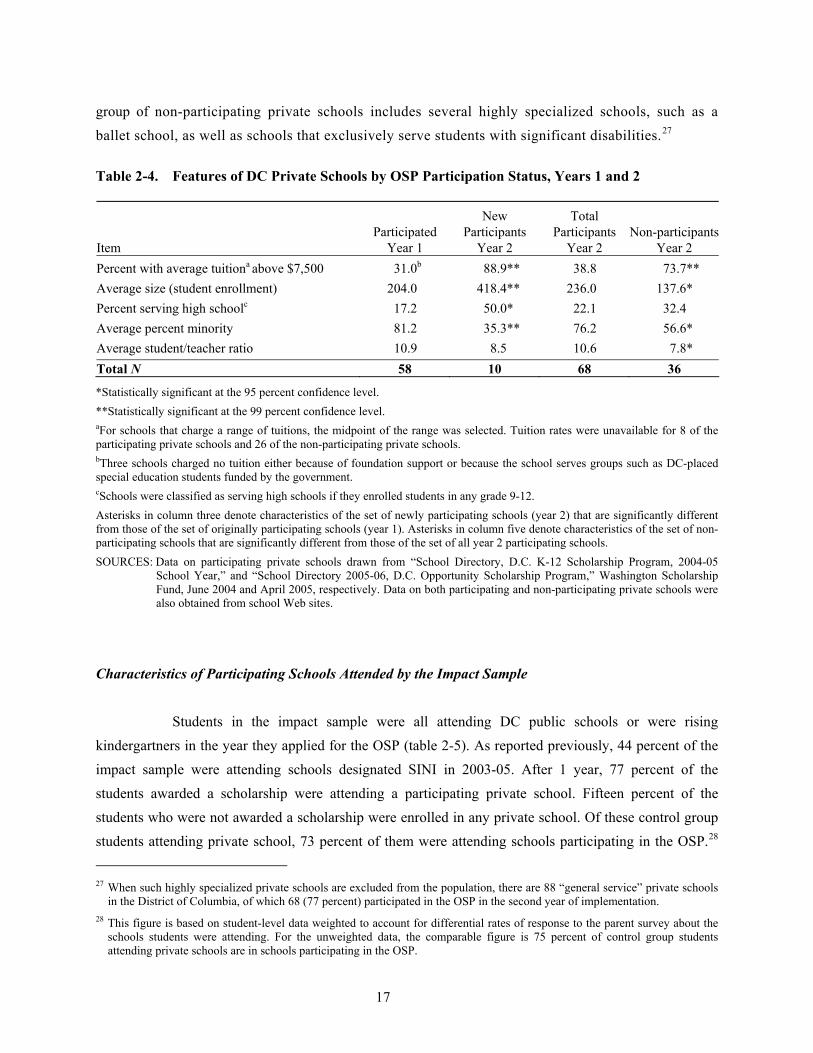
17
group of non-participating private schools includes several highly specialized schools, such as a ballet school, as well as schools that exclusively serve students with significant disabilities.27
Table 2-4. Features of DC Private Schools by OSP Participation Status, Years 1 and 2
Item Participated
Year 1
New Participants
Year 2
Total Participants
Year 2 Non-participants
Year 2 Percent with average tuitiona above $7,500 31.0b 88.9** 38.8 73.7** Average size (student enrollment) 204.0 418.4** 236.0 137.6* Percent serving high schoolc 17.2 50.0* 22.1 32.4 Average percent minority 81.2 35.3** 76.2 56.6* Average student/teacher ratio 10.9 8.5 10.6 7.8* Total N 58 10 68 36
*Statistically significant at the 95 percent confidence level. **Statistically significant at the 99 percent confidence level. aFor schools that charge a range of tuitions, the midpoint of the range was selected. Tuition rates were unavailable for 8 of the participating private schools and 26 of the non-participating private schools. bThree schools charged no tuition either because of foundation support or because the school serves groups such as DC-placed special education students funded by the government. cSchools were classified as serving high schools if they enrolled students in any grade 9-12. Asterisks in column three denote characteristics of the set of newly participating schools (year 2) that are significantly different from those of the set of originally participating schools (year 1). Asterisks in column five denote characteristics of the set of non-participating schools that are significantly different from those of the set of all year 2 participating schools. SOURCES: Data on participating private schools drawn from “School Directory, D.C. K-12 Scholarship Program, 2004-05
School Year,” and “School Directory 2005-06, D.C. Opportunity Scholarship Program,” Washington Scholarship Fund, June 2004 and April 2005, respectively. Data on both participating and non-participating private schools were also obtained from school Web sites.
Characteristics of Participating Schools Attended by the Impact Sample
Students in the impact sample were all attending DC public schools or were rising kindergartners in the year they applied for the OSP (table 2-5). As reported previously, 44 percent of the impact sample were attending schools designated SINI in 2003-05. After 1 year, 77 percent of the students awarded a scholarship were attending a participating private school. Fifteen percent of the students who were not awarded a scholarship were enrolled in any private school. Of these control group students attending private school, 73 percent of them were attending schools participating in the OSP.28 27 When such highly specialized private schools are excluded from the population, there are 88 “general service” private schools
in the District of Columbia, of which 68 (77 percent) participated in the OSP in the second year of implementation. 28 This figure is based on student-level data weighted to account for differential rates of response to the parent survey about the
schools students were attending. For the unweighted data, the comparable figure is 75 percent of control group students attending private schools are in schools participating in the OSP.
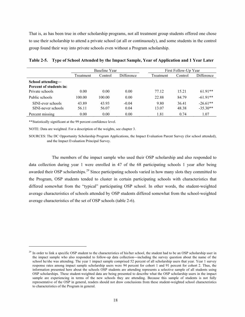
18
That is, as has been true in other scholarship programs, not all treatment group students offered one chose to use their scholarship to attend a private school (at all or continuously), and some students in the control group found their way into private schools even without a Program scholarship.
Table 2-5. Type of School Attended by the Impact Sample, Year of Application and 1 Year Later
Baseline Year First Follow-Up Year Treatment Control Difference Treatment Control Difference
School attending― Percent of students in:
Private schools 0.00 0.00 0.00 77.12 15.21 61.91** Public schools 100.00 100.00 0.00 22.88 84.79 -61.91**
SINI-ever schools 43.89 43.93 -0.04 9.80 36.41 -26.61** SINI-never schools 56.11 56.07 0.04 13.07 48.38 -35.30**
Percent missing 0.00 0.00 0.00 1.81 0.74 1.07
**Statistically significant at the 99 percent confidence level.
NOTE: Data are weighted. For a description of the weights, see chapter 3.
SOURCES: The DC Opportunity Scholarship Program Applications, the Impact Evaluation Parent Survey (for school attended), and the Impact Evaluation Principal Survey.
The members of the impact sample who used their OSP scholarship and also responded to
data collection during year 1 were enrolled in 47 of the 68 participating schools 1 year after being awarded their OSP scholarships.29 Since participating schools varied in how many slots they committed to the Program, OSP students tended to cluster in certain participating schools with characteristics that differed somewhat from the “typical” participating OSP school. In other words, the student-weighted average characteristics of schools attended by OSP students differed somewhat from the school-weighted average characteristics of the set of OSP schools (table 2-6).
29 In order to link a specific OSP student to the characteristics of his/her school, the student had to be an OSP scholarship user in
the impact sample who also responded to follow-up data collection―including the survey question about the name of the school he/she was attending. The year 1 impact sample comprised 52 percent of all scholarship users that year. Year 1 survey response rates among impact sample scholarship users were 94 percent for cohort 1 and 91 percent for cohort 2. Thus, the information presented here about the schools OSP students are attending represents a selective sample of all students using OSP scholarships. These student-weighted data are being presented to describe what the OSP scholarship users in the impact sample are experiencing in terms of the new schools they are attending. Because this sample of students is not fully representative of the OSP in general, readers should not draw conclusions from these student-weighted school characteristics to characteristics of the Program in general.

19
Table 2-6. Features of Participating Private Schools Attended by the Treatment Group
Characteristic Weighted
Mean Highest Lowest Valid N Percent of OSP students attending a school charging over $7,500 tuition
8.4 47
Tuition $5,253 $24,545 $3,400 47 Enrollment 177 1,072 5 47 Percentage of student body from racial/ethnic minority groups
95% 100% 16% 47%
Average student/teacher ratio 11.8 29.6 2.6 46 Student N 941
NOTES: “Valid N” refers to the number of schools for which information on a particular characteristic was available. When a tuition range was provided, the mid-point of the range was used. The weighted mean was generated by associating each student with the characteristics of the school he/she was attending, then computing the average of these student-level characteristics. A total of 23.7 percent of the data were missing for each of the characteristics. The private school that enrolled only five students is a Montessori school serving children in pre-K and kindergarten only.
SOURCES: National Center for Education Statistics: Private School Universe Survey, 2003-2004, supplemented by OSP School Directory information, 2004-05, 2005-06, Washington Scholarship Fund.
Only 8.4 percent of this group of OSP students was attending a school that charged tuition
above the statutory cap of $7,500 in their first year in the Program, even though 39 percent of participating schools charged tuitions above the cap by fall of 2005. The average tuition charged to these treatment group students who used their scholarships was $5,253 but varied between $3,400 and $24,545.30 The average OSP student in this group attended a school with 177 students―somewhat smaller than the average of 236 students across the set of participating schools. These OSP students are concentrated in the participating private schools with higher minority enrollments but with student/teacher ratios that are approximately representative of the entire set of OSP schools.
Most of the scholarship users in the impact sample who responded to year 1 data collection
are attending Roman Catholic schools (figure 2-3). Nearly two-thirds of these OSP students are attending the one-third of the participating OSP schools operated by the Catholic Archdiocese of Washington. About 17 percent are attending non-Catholic faith-based schools, and 18 percent are enrolled in nonsectarian private schools.
30 The WSF reported that families were not required to pay for tuition out-of-pocket in almost all cases where the tuition charged
by the school exceeded the $7,500 cap.
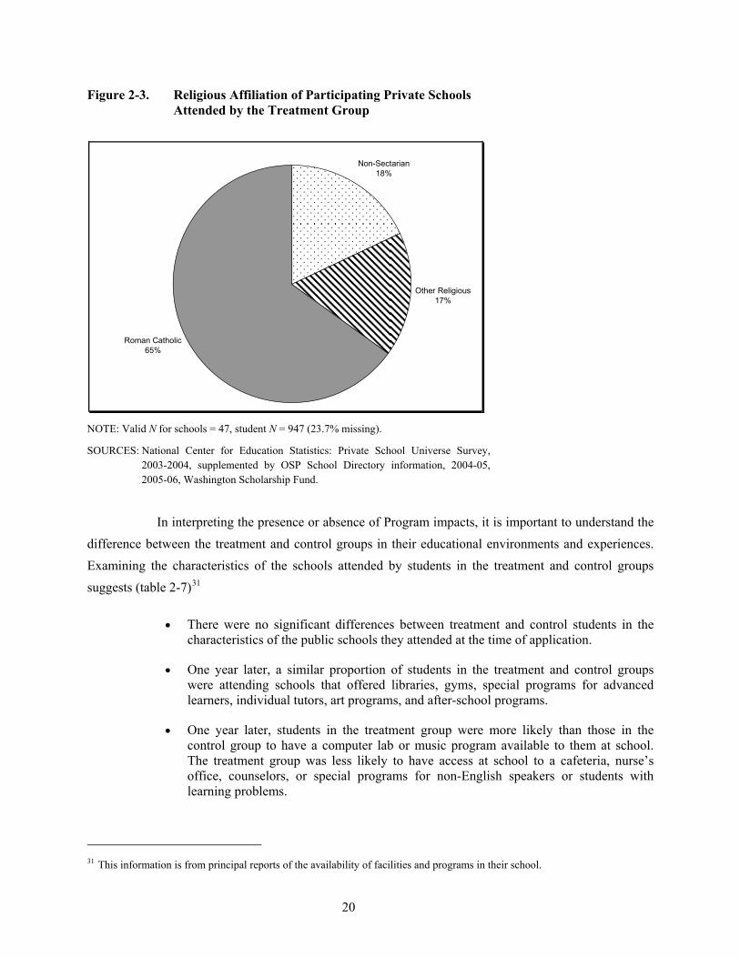
20
Figure 2-3. Religious Affiliation of Participating Private Schools Attended by the Treatment Group
Non-Sectarian18%
Other Religious17%
Roman Catholic65%
NOTE: Valid N for schools = 47, student N = 947 (23.7% missing).
SOURCES: National Center for Education Statistics: Private School Universe Survey, 2003-2004, supplemented by OSP School Directory information, 2004-05, 2005-06, Washington Scholarship Fund.
In interpreting the presence or absence of Program impacts, it is important to understand the
difference between the treatment and control groups in their educational environments and experiences. Examining the characteristics of the schools attended by students in the treatment and control groups suggests (table 2-7)31
• There were no significant differences between treatment and control students in the
characteristics of the public schools they attended at the time of application.
• One year later, a similar proportion of students in the treatment and control groups were attending schools that offered libraries, gyms, special programs for advanced learners, individual tutors, art programs, and after-school programs.
• One year later, students in the treatment group were more likely than those in the control group to have a computer lab or music program available to them at school. The treatment group was less likely to have access at school to a cafeteria, nurse’s office, counselors, or special programs for non-English speakers or students with learning problems.
31 This information is from principal reports of the availability of facilities and programs in their school.
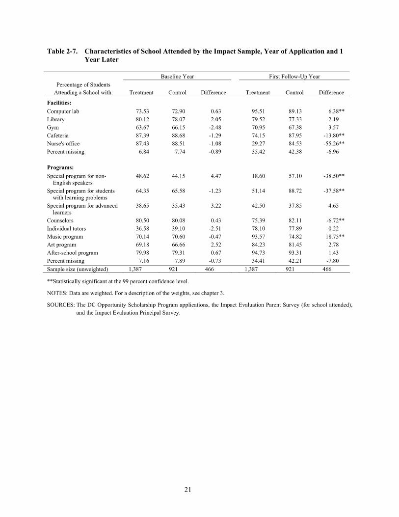
21
Table 2-7. Characteristics of School Attended by the Impact Sample, Year of Application and 1 Year Later
Baseline Year First Follow-Up Year
Percentage of Students Attending a School with: Treatment Control Difference Treatment Control Difference
Facilities: Computer lab 73.53 72.90 0.63 95.51 89.13 6.38** Library 80.12 78.07 2.05 79.52 77.33 2.19 Gym 63.67 66.15 -2.48 70.95 67.38 3.57 Cafeteria 87.39 88.68 -1.29 74.15 87.95 -13.80** Nurse's office 87.43 88.51 -1.08 29.27 84.53 -55.26** Percent missing 6.84 7.74 -0.89 35.42 42.38 -6.96
Programs: Special program for non-
English speakers 48.62 44.15 4.47 18.60 57.10 -38.50**
Special program for students with learning problems
64.35 65.58 -1.23 51.14 88.72 -37.58**
Special program for advanced learners
38.65 35.43 3.22 42.50 37.85 4.65
Counselors 80.50 80.08 0.43 75.39 82.11 -6.72** Individual tutors 36.58 39.10 -2.51 78.10 77.89 0.22 Music program 70.14 70.60 -0.47 93.57 74.82 18.75** Art program 69.18 66.66 2.52 84.23 81.45 2.78 After-school program 79.98 79.31 0.67 94.73 93.31 1.43 Percent missing 7.16 7.89 -0.73 34.41 42.21 -7.80 Sample size (unweighted) 1,387 921 466 1,387 921 466
**Statistically significant at the 99 percent confidence level.
NOTES: Data are weighted. For a description of the weights, see chapter 3.
SOURCES: The DC Opportunity Scholarship Program applications, the Impact Evaluation Parent Survey (for school attended), and the Impact Evaluation Principal Survey.

23
3. Research Methodology
The evaluation of the DC Opportunity Scholarship Program (OSP) is designed as a randomized control trial (RCT) or experiment. Experimental evaluations take advantage of a randomization process that divides a group of potential participants into two statistically similar groups―a treatment group that receives admission to the intervention or program and a control group that does not receive admission―with the control group’s subsequent experiences indicating what probably would have happened to the members of the treatment group in the absence of the intervention. Most analyses of experimental data use covariates measured at baseline in statistical models to improve the precision of the impact estimates. The results can then be interpreted in relatively straightforward ways as revealing the actual impact of the program on outcomes of policy interest. This chapter describes the central features of the evaluation’s research design, the sources and treatment of data (including why and how the data were adjusted to maintain sample balance), and how the data were analyzed in order to identify program impacts.
3.1 The “Treatment” and the “Counterfactual”
The primary purpose of this evaluation is to assess the impact of the DC Opportunity Scholarship Program. The impact is defined as the difference between outcomes observed for scholarship awardees and what would have been observed for these same students had they not been awarded a scholarship. Although it is impossible to observe the same individuals in these two different situations, if random assignment is well implemented, the students who were offered scholarships will not differ in any systematic or unmeasured way from the group of non-awardees, except for the fact that they were offered scholarships. More precisely, there may be some non-programmatic differences between the two groups, but the expected or average value of these differences is zero because they are the result of mere chance. Under this design, a simple comparison of outcomes for the two groups yields an unbiased estimate of the effect of the treatment condition, in this case an unbiased estimate of the impact of the OSP on various outcomes of interest.
It is important, however, to keep in mind the precise definition of the treatment and what it is
being compared to (referred to as the counterfactual) because it is the difference in outcomes under these two conditions that leads to the estimated impact of the Program.
24
• The treatment is the award or offer of an Opportunity Scholarship, which is all the Program can do. The Program does not compel students to actually use the scholarship or make them move from a public to a private school. Therefore, the Program’s estimated average impact includes the reality that some students who are offered a scholarship will, in fact, be disinclined to use it (what we refer to as “decliners”).
• In the same way, the counterfactual or control group condition is defined as applying for, but not being awarded, an Opportunity Scholarship. Students randomized into this group are not prevented from moving to a private school on their own, if the family opts to use its own resources or if the student is able to obtain another type of scholarship from an entity other than WSF. Such independent access to a private school education, or to a non-Opportunity Scholarship, is not a violation of random assignment but a correct reflection of what probably would have happened in the absence of the new Program, i.e., that some students in the applicant pool would have found a way to attend a private school on their own.
While these two study conditions and their comparison represent the main impact analysis approach, often called the “intent-to-treat” (ITT) analysis, the evaluation also provides separate estimates of the impact of the OSP on that subset of children who actually used the scholarship, referred to as estimated “impacts-on-the-treated (IOT).” In addition, the evaluation estimates the effects of actually attending a private school, regardless of whether an OSP scholarship is used.
3.2 Study Power
To ensure that the experimental evaluation of program impact will produce reliable findings, the sample size must be large enough to enable the analysis to answer the study’s central questions and to measure program effects that are large enough to be both meaningful in students’ lives and relevant to policy debates about the efficacy of educational interventions. The ability of a study to do so is a function of the study’s precision or “power.”
Minimum detectable effects (MDEs) are a simple way to express the statistical precision of
an impact study design. Intuitively, a minimum detectable effect is the smallest program impact or “effect size” that could be measured with confidence given random sampling and statistical estimation error.32
32 We define a minimum detectable effect as the smallest true program impact that would have an 80 percent chance of being
detected (have 80 percent power) using a two-tail hypothesis test at the 0.05 level of statistical significance. We use a two-tail test because it is conceivable that the scholarship program could have either a negative or positive effect on test scores, even though the policy question is about improved test scores.
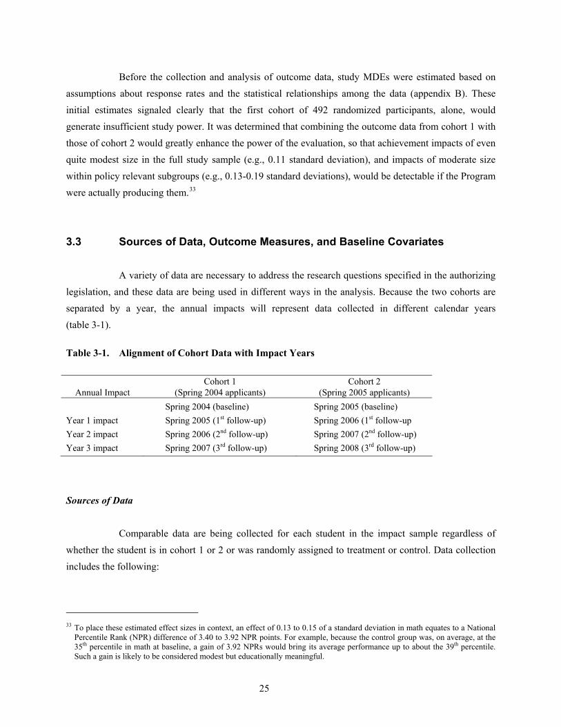
25
Before the collection and analysis of outcome data, study MDEs were estimated based on assumptions about response rates and the statistical relationships among the data (appendix B). These initial estimates signaled clearly that the first cohort of 492 randomized participants, alone, would generate insufficient study power. It was determined that combining the outcome data from cohort 1 with those of cohort 2 would greatly enhance the power of the evaluation, so that achievement impacts of even quite modest size in the full study sample (e.g., 0.11 standard deviation), and impacts of moderate size within policy relevant subgroups (e.g., 0.13-0.19 standard deviations), would be detectable if the Program were actually producing them.33
3.3 Sources of Data, Outcome Measures, and Baseline Covariates
A variety of data are necessary to address the research questions specified in the authorizing legislation, and these data are being used in different ways in the analysis. Because the two cohorts are separated by a year, the annual impacts will represent data collected in different calendar years (table 3-1).
Table 3-1. Alignment of Cohort Data with Impact Years
Annual Impact Cohort 1
(Spring 2004 applicants) Cohort 2
(Spring 2005 applicants) Spring 2004 (baseline) Spring 2005 (baseline) Year 1 impact Spring 2005 (1st follow-up) Spring 2006 (1st follow-up Year 2 impact Spring 2006 (2nd follow-up) Spring 2007 (2nd follow-up) Year 3 impact Spring 2007 (3rd follow-up) Spring 2008 (3rd follow-up)
Sources of Data
Comparable data are being collected for each student in the impact sample regardless of whether the student is in cohort 1 or 2 or was randomly assigned to treatment or control. Data collection includes the following:
33 To place these estimated effect sizes in context, an effect of 0.13 to 0.15 of a standard deviation in math equates to a National
Percentile Rank (NPR) difference of 3.40 to 3.92 NPR points. For example, because the control group was, on average, at the 35th percentile in math at baseline, a gain of 3.92 NPRs would bring its average performance up to about the 39th percentile. Such a gain is likely to be considered modest but educationally meaningful.
26
• Student assessments. Baseline measures of student achievement in reading and math for public school applicants came from the SAT-9 standardized assessment administered by the DCPS as part of its spring testing program for cohort 1 and from the SAT-9 standardized assessment administered by the evaluation team in the spring for cohort 2.34 Each spring after the baseline year, the evaluation team is administering the SAT-9 to all cohort 1 and 2 students who were offered a scholarship as well as all members of the control group who did not receive a scholarship. The testing takes place primarily on Saturdays, during the spring, in locations throughout the city arranged by the evaluators. The testing conditions are similar for members of the treatment and control groups, and the test administrators hired and trained by the evaluation team do not know whether specific students are members of the treatment or control groups. The standardized testing in reading and math provides the outcome measures for student achievement.
• Parent surveys. The OSP application included baseline surveys for parents applying to the program. These surveys were appended to the OSP application form, and therefore were completed at the time of application to the Program.35 Each spring after the baseline year, surveys of parents of all applicants are being conducted at the Saturday testing events, while parents are waiting for their children to complete their outcome testing. The parent surveys provide the self-reported outcome measures for parental satisfaction and safety. Other topics include reasons for applying, school involvement, educational climate, and curricular offerings at the school.
• Student surveys. Each spring after the baseline year, surveys of students in grades 4 and above are being conducted at the outcome testing events. The student surveys provide the self-reported outcome measures for student satisfaction and safety. Additional topics include attitude toward school, school environment, friends and classmates, and individual activities.
34 For cohort 1 at baseline, students in grades not tested by DCPS were contacted by the evaluation team and asked to attend
Saturday testing events where the SAT-9 was administered to them. Fill-in baseline test scores were obtained for 70 percent of the targeted students. Combined with the scores received from DCPS, baseline test scores were obtained from 76 percent of the cohort 1 impact sample in reading and 77 percent in math. In the school year for which cohort 2 families applied for the OSP, the DCPS assessment program was in transition, and fewer grades were tested. As a result, the evaluation team attempted to administer the SAT-9 to all eligible applicants entering grades kindergarten through 12 at Saturday testing sessions in order to obtain a comprehensive and comparable set of baseline test scores for this group. Baseline test scores were obtained from 72 percent of the cohort 2 impact sample in reading and 83 percent in math. Baseline test score response rates in reading were 79 percent for the cohort 1 treatment group and 73 percent for the cohort 1 control group, a difference of 6 percentage points. In math, the cohort 1 treatment response rate at baseline was 80 percent—7 percentage points above the control rate of 73 percent. For cohort 2, baseline test score response rates were lower for the treatment group than for the control group in reading—72 percent compared to 73 percent—but higher in math—84 percent for the treatment group versus 81 percent for the control group. For the combined cohort impact sample, the baseline response rates in reading were 73 percent for both the treatment and control groups. In math, the combined cohort response rate was 83 percent for the treatment group and 79 percent for the control group. Although the SAT-9 is not available for students below first grade, Stanford Achievement does offer similar tests that are vertically equated to the SAT-9 for younger students. We administered these tests—the SESAT 1 for rising kindergartners and the SESAT 2 for current kindergartners (i.e., rising first graders).
35 The levels of response to the baseline parent surveys varied somewhat by item. All study participants provided complete baseline data regarding characteristics that were central to the determination of eligibility and priority in the lottery, such as family income and grade level. Response rates were very high (98-99 percent) for baseline survey items associated with the basic demographic characteristics of participating students, such as age, race, ethnicity, and number of siblings. Baseline survey response rates were lower (85-86 percent) for items concerned with the education and employment status of the child’s mother. The baseline survey response rates for the treatment and control groups did not differ systematically.
27
• Principal surveys. Each spring, surveys of principals of all public and private schools operating in the District of Columbia are being conducted. Topics include self-reports of school organization, safety, climate, principals’ awareness of and response to the OSP, and, for private school principals, why they are or are not participating in the OSP. Information from the principal surveys will be analyzed in future reports to describe what is happening within the public and private schools in DC, possibly as a result of the operation of the OSP. In addition, in later reports information from principals of impact sample members (treatment and control group) will be used to assess the relationship between school characteristics and impacts.
Outcome Measures
Congress specified in the Program statute that the rigorous evaluation study possible impacts regarding academic achievement, school safety, and satisfaction. For this first year impact report, impact estimates were produced for all three of these outcome domains: (1) academic achievement (two measures); (2) parent self-reports of school safety (one measure) and student self-reports of school safety (one measure); and (3) parental self-reports of satisfaction (three measures) and student self-reports of satisfaction (three measures). As in this report, previous studies of scholarship program impacts have used multiple measures of the outcomes of interest because achievement, safety, and satisfaction are constructs that often cannot be measured completely or well using any single indicator (see Mayer et al., 2002; Witte, 2001). All outcome data were obtained from impact sample respondents in the spring of their first year after random assignment and include the following:
• Academic outcomes. The academic outcomes used in these analyses are assessments
of student academic achievement in reading/language arts and mathematics derived from the administration of the Stanford Achievement Test, 9th Edition (SAT-9) by Westat-trained staff.36 Like most norm-referenced tests, the SAT-9 includes subtests within the reading and math domains in most grades; e.g., in grades 3-8, the reading test comprises reading vocabulary and reading comprehension, while the math test consists of math problem solving and math procedures. This norm-referenced test is designed to measure how a student’s performance compares with the scores of other students who took the test for norming purposes.37 Each student’s performance is measured using scale-scores that are derived from item response theory (IRT) item-pattern scoring methods, which use all of the information contained in a student's pattern of item responses to compute an individual’s score. These scores have an
36 The law requires the evaluation to use as its academic achievement measure the same assessment DCPS was using the first
year the OSP was implemented, which was the SAT-9. 37 The norming sample for the SAT-9 included students from the Northeastern, Midwestern, Southern, and Western regions of
the United States and is also representative of the Nation in terms of ethnicity, urbanicity, socio-economic status, and students enrolled in private and Catholic schools. The norming sample is representative of the Nation, but not necessarily of DC or of low-income students. Scale scores are vertically integrated across grades, so that scores tend to be higher in the upper grades and lower in the lower grades. For example, the mean and standard deviation (SD) for the norming population is 463.8 (SD=38.5) for kindergartners tested in the spring, compared to 652.1 (SD=39.1) for fifth graders and 703.6 (SD=36.5) for students in twelfth grade.
28
additional property called “vertically equating,” which allows scores to be compared across a grade span (e.g., K-12) to measure changes over time (see appendix C).
• Parent self-reports of school safety. Parents were asked about the perceived seriousness of a number of problems at their child’s school commonly associated with danger and rule-breaking. The specific items, all drawn from the surveys used in previous experimental evaluations of scholarship programs, were:
– Property destruction; – Tardiness; – Truancy; – Fighting; – Cheating; – Racial conflict; – Weapons; – Drug distribution; – Drug and alcohol use; and – Teacher absenteeism.
Parents were asked to label these conditions as “very serious,” “somewhat serious,” or “not serious” at their child’s school. Responses to these items subsequently were categorized as “yes” (very or somewhat serious) or “no” (not serious). The number of “yes” responses for each parent were then summed to create a parental danger index or count that ranged from 0 to 10.38
• Student self-reports of school safety. Students were asked how often (never, once or twice, three times or more) various adverse events had occurred to them this school year. The student danger indicators, drawn from previous scholarship program evaluations, included instances of:
– Theft; – Being offered drugs; – Physical assault; – Threats of physical harm; – Observations of weapons being carried by other students; and – Bullying.
38 Previous experimental evaluations of scholarship programs used summary scales to measure parental satisfaction, as we do
below, but generally presented parental and student danger outcomes and student satisfaction outcomes for the individual items that we list here. We have created scales of satisfaction and indexes of danger concerns because the outcome patterns for the individual items tend to be generally consistent and, under such conditions, scaling them or combining them in indices tends to generate more reliable results (see appendix D). The impacts of the Program on each individual item in the various scales and indices are discussed in each section of chapter 4 that reports impacts on scaled outcomes.
29
Responses to these items were categorized as “yes” (at least once) or “no” (never) to create a count of the number of reported events that ranged from 0 to 6 (see Spector, 1992).39
• Parental self-reports of satisfaction. Parent satisfaction with their child’s school was measured three ways. First, parents were asked “What overall grade would you give this child’s current school?” Two outcomes were created from this question: (1) a 5-point grading scale ranging from 1 (an F) to 5 (an A) and a dichotomous variable equal to 1 if the parent assigned an A or B, and equal to zero otherwise.
In addition, parents were asked “How satisfied are you with the following aspects of your child’s school?” and to rate each of the following dimensions on a 4-point scale ranging from “very dissatisfied” to “very satisfied:”
– Location of school; – School safety; – Class sizes; – School facilities; – Respect between teachers and students; – How much teachers inform parents of students’ progress; – How much students can observe religious traditions; – Parental support for the school; – Discipline; – Academic quality; – Racial mix of students; and – Services for students with special needs.
The responses to this set of items were combined into a single parent satisfaction scale using maximum likelihood IRT. IRT is a procedure which draws upon the complete pattern of responses to a set of questions in order to develop a reliable gauge of the respondent’s level of a “latent” or underlying trait, in this case satisfaction (Hambleton, Swaminathan, and Rogers, 1991). (See appendix D for a more detailed description of IRT.) In situations such as exist here, when individual questions each capture some piece of a more general construct (e.g., satisfaction) and the response categories capture the degree as well as the direction of the response, the IRT method is superior to count-based indices in measuring subjective conditions or traits. Two specific advantages of IRT scoring are that: (1) it allows scores to be assigned in the event that a respondent missed one of the scale items in his/her response, and (2) it identifies specific items that are highly effective in distinguishing respondents and assigns more weight to those items in the scale. For example, the IRT method is commonly used to score standardized tests. It will identify the questions that most clearly separate the better performing students from the worse performing students and count those items more heavily in generating the final test scores.
39 As a count of discrete items, the student school danger index and the similar index from parent reports were not subject to
internal consistency checks using Cronbach’s Alpha. The sum of item counts lacks multi-dimensional features of summated scale items, such as both direction and degree, that generate the data patterns necessary to produce consistency ratings.

30
The consistency and reliability of scaled measures of traits such as satisfaction can be determined by a rating statistic called Cronbach’s Alpha (Spector, 1992).40 The completed parent satisfaction scale exhibited very high consistency with a Cronbach’s Alpha of 0.938.
• Student self-reports of satisfaction. Students were also asked to grade their school using the same question asked of parents, and two outcomes were created―a grade range and a dichotomous variable―as discussed above for parents. Students were similarly asked to rate various specific aspects of their current school on a 4-point scale. The individual items covered the following topics (see appendix D):
– Behavior and discipline; – Academic quality; – Social supports and interactions; and – Teacher quality.
A single composite satisfaction scale was created for students using the same IRT procedures used to create the parent satisfaction scale. The student scale exhibited somewhat lower consistency with a Cronbach’s Alpha of 0.814, still well within the range of acceptable reliability.
Baseline or “Preprogram” Covariates
In addition to the collection of outcome data for each study participant, various personal, family, and educational characteristics of the students in the impact sample were obtained prior to random assignment via the application form (including a parent survey) and administration of the SAT-9 in reading and math (see appendix E).41 Such “baseline” covariates are important in the context of an experimental evaluation, because they permit researchers to (1) verify the integrity of the random assignment (see chapter 2), (2) inform the generation of appropriate non-response weights, and (3) include the covariates in regressions to improve the precision of the estimations of treatment impacts and adjust for any baseline differences across the treatment and control groups (for a spirited exchange on this question, see Howell and Peterson, 2004; Krueger and Zhu, 2004a, 2004b, Peterson and Howell, 2004.42 The covariates that are most useful in performing each of these three functions are those that previous research has linked to the study outcomes of interest (Howell and Peterson et al., 2002, p. 212).43 These
40 J. C. Nunnally is credited with developing the widely accepted standard that a Cronbach’s Alpha above .70 demonstrates an
acceptable degree of internal consistency for a multi-item scale. 41 Cohort 1 baseline test scores were obtained from the DCPS accountability testing database. Because DCPS dropped the SAT-9
as its accountability test in 2005, baseline test scores for cohort 2 were obtained through SAT-9 administration by Westat. 42 Analysts tend to agree that baseline covariates are useful in these ways within the context of an RCT, although some of them
disagree regarding which of the three functions of preprogram covariates is most important. 43 Previous analysts of voucher experiments have used a similar set of baseline covariates to estimate attendance at outcome data
collection events and therefore inform student-level non-response weights.
31
variables regularly are included in regression models designed to estimate educational outcomes such as test scores, or, in the case of the SINI indicator, are especially important to this particular evaluation (see Krueger and Zhu, 2004a, p. 692):44
• Student’s baseline reading scale score,
• Student’s baseline math scale score,
• Student attended a school designated SINI 2003-05 indicator,
• Student’s age (in months) at the time of application for an Opportunity Scholarship,
• Student’s forecasted entering grade for the next school year,
• Student’s gender – male indicator,
• Student’s race – African American indicator,
• Special needs indicator – whether the parent reported that the student has a disability,
• Mother has a high school diploma indicator (GED not included),
• Mother has a 4-year college degree indicator,
• Mother employed either full or part time indicator,
• Household income―reported total annual income,
• Total number of children in student’s household, and
• Stability―the number of months the family has lived at its current address.
3.4 Sampling and Non-Response Weights
Sampling weights were used in the impact analyses to account for the fact that the study sample was selected differently in the 2 years of OSP implementation as well as across different priority groups and grade bands (see section 2.2). Conducting the analyses without weights would run the risk of confusing the effect of the treatment with compositional differences between the treatment and control groups due to the fact that certain kinds of eligible applicants had higher or lower probabilities of being
44 This list of baseline covariates is almost identical to the one that Krueger and Zhu used in one of their re-analyses of the data
from the New York City voucher experiment. The only differences include alternate measures of the same characteristic (e.g., our measure of student disability includes English language learners whereas Krueger and Zhu included a separate indicator for English spoken at home) or variables that we were not able to measure at baseline (e.g., mother’s religion and mother’s place of birth).
32
awarded a scholarship. The sampling weights consist of two primary parts: (1) a “base weight,” which is simply the inverse of the probability of being selected to treatment (or control) and (2) an adjustment for differential non-response to data collection. (See appendix F for a more detailed explanation of the calculation of these weights.)
3.5 Analytical Model for Estimating the Impact of the Program, or the Offer of a Scholarship (Experimental Estimates)
To estimate the extent to which the Program has an effect on participants, this study first compares the outcomes of the two experimental groups created through random assignment, or the ITT approach referred to earlier in this chapter. The only completely randomized and therefore strictly comparable groups in the study are those students who were offered scholarships (the treatment group) and those who were not offered scholarships (the control group) based on the lottery. The random assignment of students into treatment and control groups should produce groups that are similar in key characteristics, both those we can observe and measure (e.g., family income, prior academic achievement) and those we cannot (e.g., motivation to succeed or benefit from the program). A comparison of these two groups is the most robust and reliable measure of Program impacts because it requires the fewest assumptions and least effort to make the groups similar except for their participation in the Program.
Overall Program Impacts
Because the RCT approach has the important feature of generating comparable treatment and control groups, we used a common set of analytic techniques, designed for use in social experiments, to estimate the Program’s impact on test scores and the other outcomes listed above. These analyses began with the estimate of simple mean differences using the following equation, illustrated using the test score of student i in year t (Yit ):
(1) Yit =α+ τ Tit + εit if t>k (period after program takes effect),
where Tit is equal to 1 if the student has the opportunity to participate in the scholarship Program (i.e., the award rather than the actual use of the scholarship) and is equal to 0 otherwise. Equation (1) therefore estimates the effect of the offer of a scholarship on student outcomes. Under this ITT model, all students who were randomly assigned by virtue of the lottery are included in the analysis, regardless of whether a member of the treatment group used the scholarship to attend a private school or for how long.
33
Proper randomization renders experimental groups approximately comparable, but not necessarily identical. In the current study, some modest differences, almost all of which are not significant, exist between the treatment group and the control group counterfactual at baseline (see Krueger and Zhu, 2004a; Peterson and Howell, 2004).45 The basic regression model can, therefore, be improved by adding controls for observable baseline characteristics to increase the reliability of the estimated impact by accounting for minor differences between the treatment and control groups at baseline and improving the precision of the overall model.
This yields the following equation to be estimated: (2)Yit =α+ τ Tit + Xi γ+ δR Rit+ δM Mit+ εit.
where Xi is a vector of student and/or family characteristics measured at baseline and known to influence future academic achievement, and Rit and Mit refer to baseline reading and mathematics scores, respectively (each of the included covariates are described below). In this model, τ―the parameter of sole interest―represents the effect of scholarships on test scores for students in the program, conditional on Xi and the baseline test scores. The δ’s reflect the degree to which test scores are, on average, correlated over time. With a properly designed RCT, baseline test scores and controls for observable characteristics that predict future achievement should improve the precision of the estimated impact.
45 For example, although the average test scores of the cohort 1 and cohort 2 treatment and control groups in reading and math
are all statistically comparable, in all four possible comparisons (cohort 1 reading, cohort 1 math, cohort 2 reading, cohort 2 math) the control group average baseline score is higher. That is, on average the members of the control group began the experiment with slightly higher reading and math test scores than the members of the treatment group. The control group baseline test score advantage for cohort 1 reading, cohort 2 reading, cohort 1 mathematics, and cohort 2 mathematics was 4.7, 8.4, 4.1, and 8.7 respectively, when the pre-imputation scores were used. The corresponding four differences were 4.1, 7.0, 3.7, and 1.6 when the post-imputation scores were used. Thus, after imputation the differences between treatment and control group baseline scores were attenuated. A joint f-test for the significance of the pattern of test score differences at baseline was not significant for the pre-imputation data but was significant using the post-imputation scores. This apparent anomaly is a result of the larger sample sizes after imputation, which reduces the standard errors across the board, thereby increasing the precision of the statistical test and the resulting likelihood of a statistically significant result. To deal with this difference in test scores across the treatment condition at baseline, we simply include the post-imputation baseline test scores in a statistical model that produces regression-adjusted treatment impact estimates. Controlling for baseline test scores in this way effectively transforms the focus of the analysis from one on achievement levels after 1 year, which could be biased by the higher average baseline test scores for the control group, to one on comparative achievement gains after 1 year from whatever baseline the individual student performed at to start the experiment. Because including baseline test scores in regression models both levels the playing field in this way and increases the precision of the estimate of treatment impact, it is a common practice in education evaluations generally and school scholarship experiments particularly.
34
Adjustment for Differences in Days of Exposure to School
A final important covariate to include in this model is the number of days from September 1 to the date of outcome testing for each student.46 This “days until test” variable, signified by DT in the equation below, controls for the fact that test scores were obtained over a 4-month period each spring and that a student’s ability to perform on the standardized tests can be affected by the length of time he/she has been exposed to schooling. The “days until test” variable was further interacted with elementary school status (i.e., K-5), because younger students tend to gain relatively more than older students from additional days of schooling.47 Thus, the models that produced the regression-adjusted impact estimates for this analysis took the general form:48
(3)Yit =α+ τ Tit + Xi γ+ δR Rit+ δM Mit+ δDTDTit + εit. The same set of baseline covariates and the days-until-test variable were used in all
regression models, regardless of whether student achievement, school satisfaction, or school safety outcomes were being estimated.49
Subgroup ITT Impacts
In addition to estimating overall program impacts, this study was interested in the possibility of heterogeneous impacts (i.e., separate impacts on particular subgroups of students). Subgroup impacts were estimated by augmenting the basic analytic equation (3) to allow different treatment effects for different types of students, as follows:
46 September 1st was chosen as a common reference date because most private schools approximately follow the DCPS academic
calendar, and September 1st fell within the first week of schooling in fall of both 2004 and 2005. 47 The actual statistical results confirmed the validity of this assumption, as the effect of the days-until-test variable on outcome
test scores was positive and statistically significant for K-5 students but indistinguishable from zero for 6-12 students. 48 The possibility of a nonlinear relationship of days-until-test with the outcome variables was examined through the use of a
categorized version of the days-until-test variable, with one category level including students with days-until-test below the median value, one level with days-until-test in the third quartile (median to 75th percentile), and one level with days-until-test in the fourth quartile (75th percentile to maximum). This allows for a quadratic relationship (down-up-down for example) in the regression estimation if such a relationship exists. The regression with the nonlinear days-until-test component did not provide a better fit to the data than the regression modeling a simple linear slope. As a result, the simpler model was used.
49 After the initial impacts were obtained, a second set of estimates were run to test the sensitivity of the results to the set of covariates included in the model. This sensitivity model used only cohort, grade, special needs, number of children in the household, African American race, baseline reading, baseline math, and days until test as control variables, as these variables tended to be significant predictors of test score outcomes in the first set of models. No important differences were found.
35
(4) Yikt = μ+ τTikt + τB Pi*Tikt +∑bj=2 ϕj
is + Xik γ+ δR Rit+ δM Mit+ δDTDTit + εik,t
where P is an index for whether a student is a member of a particular subgroup (the P must be part of the X’s). The coefficient τP indicates the marginal treatment effect for students in the designated subgroup. These models were used to estimate impacts on the separate components of the subgroup (e.g., impacts on males and females separately), and the difference in impacts between the two groups. These analyses of possible heterogeneous impacts across subgroups are conducted within the context of the experimental ITT design. Thus, as with the estimation of general program-wide impacts, any subgroup-specific impacts identified through this approach are understood to have been caused by the treatment. The ability to reliably identify separate impacts, however, depends on the sample sizes within each subgroup. Consequently, subgroup impacts were estimated for the following groups:
• Applied from a school ever designated SINI―yes and no;
• Academically lower performing student at the time of baseline testing (i.e., bottom one-third of the test score distribution) and higher performing (top two-thirds);50
• Gender―male and female;
• Grade band―K-8 and high school; and
• Cohort―1 and 2.
Computation of Standard Errors
In computing standard errors it is necessary to factor in the stratified sample design, clustering of student outcomes within individual families, and non-response adjustments. As a consequence, all of the impact analyses were completed using sampling weights in STATA.51 The effects of family clustering, which is not part of the sample design, but which may be having a measurable effect
50 The lower third of the baseline performance distribution was chosen because preliminary power analyses suggested it would be
the most disadvantaged performance subgroup that would include a sufficient number of members to reveal a distinctive subgroup impact if one existed.
51 There is also a positive effect on variance (a reduction in standard errors) from the stratification. This effect will not be captured in the primary analyses, making the resultant variance estimators conservative. We will compute variances including the stratification directly via the use of jackknife replicate weights and also using Taylor-series linearization via STATA, but this will be a secondary analysis designed to confirm that the main analysis variances are not excessively conservative.
36
on variance, were taken into account using robust regression calculations (i.e., “sandwich” variance estimates) (see Liang and Zeger, 1986; White, 1982).52 3.6 Analytical Model for Estimating the Impact of Using a Scholarship and
of Attending a Private School
Although the ITT analysis described above is the most reliable estimate of Program impacts, it cannot answer the full set of questions that policymakers have about the effects of the Program. Two different techniques, which deviate to different extents from the random assignment design, are necessary to estimate the impact on students and families from using a scholarship or from attending a private school (see appendix G for a more detailed discussion of the analytic methods, including the equations used in the models).
Impact of Using a Scholarship
For the scholarship awardees in the OSP impact sample that provided year 1 outcome test scores and the name of their school, 80 percent were attending a private school.53 The 20 percent of the treatment students who did not use their scholarships are treated the same as scholarship users for purposes of determining the effect of the offer of a scholarship, so as to preserve the integrity of the random assignment, even though scholarship decliners likely experienced no impact from the Program. Fortunately, there is a way to estimate the impact of the OSP on the average participant who actually used a scholarship, or what we refer to as the “impact-on-the-treated” (IOT) estimate. This approach does not require information about why 20 percent of the individuals declined to use the scholarship when awarded, or how they differ from other families and children in the sample. But if one can assume that
52 We also examined the effect on the standard errors of the estimates of clustering on the school students attended at baseline.
Baseline school clustering reduced the standard errors of the various impact estimates by an average of 2 percent, compared to an average reduction of less than 1 percent due to clustering by family. These results indicate that the student outcome data are almost totally independent of the most likely sources of outcome clustering. They may appear to be counter-intuitive, since formally accounting for clustering among observations usually increases variance in effects; however, since the randomization cut across families and baseline schools, it is possible that family and school clusters served as the equivalent of random-assignment blocks, as most multi-student families and schools contained some treatments and some controls. Such circumstances normally operate to reduce variance in subsequent impact estimates, as the within-cluster positive correlation comes into the calculation of the variance of the treatment-control difference with a minus sign. This last point is a technical matter that we plan to explore in greater depth in the future.
53 A total of 17 treatment students who took the follow-up test in math (1.6 percent) and 7 treatment students who outcome tested in reading did not identify their current school. Since these observations represent less than 2 percent of the impact sample, the evaluators simply excluded them from the portion of the analysis focused on the impact of treatment on the treated and the effect of private schooling.
37
decliners experience zero impact from the scholarship Program―which seems reasonable given that they did not use the scholarship, it is possible to avoid these kinds of assumptions about (or analyses of) selection into and out of the Program.
This is possible by using the original comparison of all treatment group members to all
control group members (i.e., the ITT estimates described above) but re-scaling it to account for the fact that a known fraction of the treatment group members did not actually avail themselves of the treatment and therefore experienced zero impact from the treatment. The average treatment impact that was generated from a mix of treatment users and nonusers is attributed only to the treatment users, by dividing the average treatment impact by the proportion of the treatment group who used their scholarships. For this report, depending on the specific outcome being rescaled, this “Bloom adjustment” (Bloom, 1984) will increase the size of the ITT impacts by 25-35 percent, since the percentage of treatment users among the population of students that provided valid scores on the various test and survey outcomes ranged from 74-80 percent.
In the current evaluation, conventional Bloom adjustment may not be sufficient to accurately
estimate the impact of using the OSP scholarship. It is conceivable that the design of the OSP Program and lotteries made it possible for some control group members to attend participating private schools, above and beyond the rate at which low-income students would have done so in the absence of the Program. Statistical techniques that take this “program-enabled crossover” into account are necessary for testing the sensitivity of the evaluation’s impact estimates.
In a social experiment, even as some students randomized into the treatment group will
decline to use the treatment, some students randomized into the control group will obtain the treatment outside of the experiment. For example, in medical trials, this control group “crossover” to the treatment can occur when the participants in the control group purchase the equivalent of the experimental “treatment” drug over the counter and use it as members of the treatment group would. The fact that crossovers have obtained the treatment does not change their status as members of the control group―just as treatment decliners forever remain treatments―for two reasons: (1) changing control crossovers to treatments would undermine the initial random assignment, and (2) control crossover typically represents what would have happened absent the experimental program and therefore is an authentic part of the counterfactual that the control group produces for comparison. If not for the medical trial, the control crossovers would have obtained the similar drug over the counter anyway. Therefore, any effect that the crossover to treatment has on members of the control group is factored into the ITT and Bloom-adjusted IOT estimates of impact as legitimate elements of the counterfactual.
38
In the case of the OSP experiment, control crossover takes place in the form of students in the control group attending private school. Among the members of the control group who provided outcome tests in math, 15 percent reported attending a private school. This crossover rate is in the higher end of the range reported for previous experimental evaluations of privately funded scholarship programs (Howell and Peterson et al., 2002, p. 44).54 The crossover rate also is higher for control group students with siblings in the treatment group (18 percent) compared to those without treatment siblings (11 percent),55 a difference that is statistically significant beyond the 99 percent confidence level. At outcome data collection events, some parents of control group students commented to evaluation staff that their control-group child was accepted into a participating private school free-of-charge because he or she had a treatment group sibling who was using a scholarship to attend that school, and private schools were inclined to serve a whole family. Thus, apparently some of the control crossover that is occurring in the OSP could be properly characterized as “Program-enabled” and not a legitimate aspect of the counterfactual.
The data suggest that 4 percent of the control group were likely able to enroll in a private
school because of the existence of the OSP. This hypothesis is derived from the fact that 11 percent of the control group students without treatment siblings are attending private schools, whereas 15 percent of the control group overall is in private schools. Since the 11 percent rate for controls without treatment siblings could not have been influenced by “Program-enabled crossover,” we subtract that “natural crossover rate” from the overall rate of 15 percent to arrive at the hypothesized Program-enabled crossover rate of 4 percent. To adjust for the fact that this small component of the control group may have actually received the private-schooling treatment by way of the Program, the estimates of the impact of scholarship use will include a “double-Bloom” adjustment. We will rescale the pure ITT impacts that are statistically significant by an amount equal to the treatment decliner rate (~20 percent), as described above and, in addition, rescale in the same manner for the possible Program-enabled crossover rate (~4 percent). This strategy will provide upper and lower bounds for the IOT estimates.
54 First-year control group crossover rates in the previous three-city experiment were 18 percent in Dayton, Ohio; 11 percent in
Washington, DC; and just 4 percent in New York City. Among those three cities, the average tuition charged by private schools is lowest in Dayton and highest in New York, a fact that presumably explains much of the variation in crossover rates.
55 Because program oversubscription rates varied significantly by grade, random assignment took place at the student and not the family level. As a result, nearly half the members of the control group have siblings who were awarded scholarships.
39
Effect of Attending a Private School
A third analysis that is made possible within the context of an experimental study is an estimation of the effect of experiencing the treatment, whether as a member of the treatment or control group. Such an analysis is conceptually distinct from estimating the IOT by way of the Bloom or “double-Bloom” adjustments described above, since it examines outcome patterns in both treatment and control groups that could be results of exposure to the treatment, either inside or outside the experiment.
Such an analysis is inherently non-experimental, since, short of mandating the use of the
scholarship by the treatment group and outlawing private schooling for the control group, there is no way to perfectly randomize scholarship use. So long as parents and students have the option of declining scholarships or obtaining private schooling outside of the experimental program, estimates of private schooling effects within the context of experiments are biased by the selective nature of scholarship users relative to all scholarship winners and control group “crossovers” relative to controls that remain in public schools.
In this setting, instrumental variable (IV) analysis provides a well-established method to
generate the best estimate of the impact of private schooling, drawing upon the ITT estimator (Howell and Peterson et al., 2002, pp. 49-51). Two stages of regression equations are run in order to arrive at an estimate of the effects of private schooling on each outcome, attempting to account for selection bias. In the first stage, the results of the treatment lottery and student characteristics at baseline are used to estimate the likelihood that individual students attended a private school in year 1. In the second stage, that estimate of the likelihood of private schooling operates in place of an actual private schooling indicator to estimate the effect of private schooling on outcomes. In cases like this experiment, the IV procedure will generate estimates of the effect of private schooling that will be slightly larger than the double-Bloom IOT impact estimates. Since the IV process places greater demands upon the data, special attention must be paid to the significance levels of IV estimates, as some experimental impacts that are statistically significant at the ITT stage lose their significance when subjected to IV analysis.


41
4. Impact of Being Awarded a Scholarship, One Year After Application
The statute that authorized the District of Columbia Opportunity Scholarship Program (OSP) mandated that the Program be evaluated with regard to its impact on student test scores and safety, as well as the “success” of the Program, which, in the design of this study, includes satisfaction with school choices. This chapter presents the effects of being awarded a scholarship on these outcomes 1 year after families and students applied to the OSP, or approximately 7 months after the start of their first possible school year in the Program. After providing some context for understanding the presentation of results, most of the chapter describes findings on the impact of the offer of a scholarship, including a discussion of subgroup impacts and checks for the sensitivity of the results. The results tables in this chapter convey information about the treatment and control group means and any difference between them (i.e., the programmatic impact) that is drawn from the regression equations described above in chapter 3. Appendix H contains a parallel set of results tables that include the raw (unadjusted) group means as well as additional statistical detail regarding the impact estimates.
4.1 Interpreting the Impacts
The impact results in the following sections are presented in a variety of ways and include a comprehensive approach to assessing the validity of the findings. First, there are tables that provide the following information for each outcome measure whenever space permits:
• Treatment group mean;
• Control group mean;
• Estimated difference in means, which is the treatment impact;
• Effect size in standard deviation units;56 and
• p-value.
56 Specifically, the effect sizes are computed as a percentage of a standard deviation for the control group after 1 year. Since the
outcomes of the experimental control group signal what would have happened to the treatment group in the absence of the intervention, a standard deviation in the distribution of the control group outcomes represents an especially appropriate gauge of the magnitude of any treatment impacts observed.
42
The means are adjusted for minor differences between the treatment and control groups at baseline. The control group mean for a given outcome is predicted from a regression equation that includes an indicator variable for the treatment impact as well as the full set of baseline covariates described in chapter 3. The treatment group mean is then generated by adding the treatment impact from the regression equation to the predicted control group mean. Conceptually, the treatment group mean expressed in this way describes what the control group mean would have looked like had the control group been administered the programmatic treatment.57 Effect sizes translate the impact into a standard metric and provide information about whether the size of the impact might be considered meaningful. Programmatic impacts might be statistically significant in that they are reliable, but might be either sizable or trivial in magnitude. Given the power levels for this evaluation, however, any impacts that are statistically significant are likely to be at least “moderate” in size for an educational intervention. The p-value gives a sense of the extent to which we can be certain that an estimated impact of the Program is reliable and not a chance anomaly. The smaller the p-value, the more confidence we can have that an observed impact is due to the treatment and not merely due to chance.
Second, these measures are also converted into a series of figures that visually demonstrate
the impact. In particular, brackets that represent the range of values that lay within a 95 percent confidence interval are placed around the impact estimate. If that range of plausible values includes the value of zero, then we cannot reject the hypothesis that the Program had no impact on that outcome.
Third, the analyses of each type of outcome (achievement, safety, satisfaction) used different
specific measures and were estimated for the overall impact sample as well as various policy-relevant subgroups of students. Under such conditions of “multiple comparisons,” there is a modest probability that a finding of a statistically significant difference will emerge by random chance―an event that is known in the statistical field as a “false discovery.” False discoveries are most common when p-values are very close to the prescribed cut-off level for statistical significance, in this case p < .05, and when many comparisons are made, thereby giving random chance extra opportunities to produce an apparently (but not actually) statistically significant finding.
57 This approach is somewhat complicated in the case of calculating the regression adjusted means—also called the predicted marginals—for analysis of subgroups. The predicted marginal is defined as the average predicted response if all the students in the entire study sample had been in a given subgroup (e.g., males). The predicted values are derived from the fitted model (either ordinary least squares (OLS) for continuous outcomes or logistic for binary outcomes), where each individual's values on the covariates are used with the exception of the subgroup of interest, which is set to 1 and to 0 for each observation. In other words, the predicted marginal calculation sets every observation in the sample as fixed (i.e., assigned the value corresponding to male), and all other variables are what was observed for each student.
43
To guard against the drawing of firm conclusions generated by false discoveries, Benjamini and Hochberg (1995) developed a statistical test designed to screen out marginally significant findings from multiple comparisons, since such results could be the product of random forces. Following those procedures, the evaluation team statistically adjusted the p-values for results that were the product of multiple comparisons to account for how many comparisons were in the set that produced the particular finding. As a result of the Benjamini-Hochberg test, a few findings that initially appeared to be barely statistically significant, but were part of a set of subgroup or item-specific findings generally NOT found to be statistically significant, were downgraded to not statistically significant in the interest of guarding against false discoveries. Individual findings that were highly statistically significant or were a part of a group of findings that all were statistically significant were not affected in any substantive way by this adjustment.
Finally, in any evaluation, decisions are made about how to handle certain data or analysis
issues (e.g., missing data, sampling weights, etc.). While there are some commonly accepted approaches in research and evaluation methodology, sometimes there are multiple approaches, and any could be acceptable. The evaluation team chose its approach in consultation with a panel of methodology experts before analyzing the data and seeing the results. However, in an effort to be both transparent and complete, each presentation of analysis is followed by a discussion of the sensitivity testing conducted to determine how robust the estimates are to alternative specifications or analytic approaches. These alternative specifications include:
• Trimmed sample: The sample of students was trimmed back to equalize the actual
response rates of the treatment and control groups. Since the actual response rate of the treatment group was higher (79 percent), in effect the “latest treatment group members to respond” were dropped from the sample until the treatment response rate matched the control group’s pre-subsample response rate of 68 percent. This is an alternative to the primary analysis, where all observations were used even though a higher percentage of the treatment than the control group responded to outcome data collection. This sensitivity testing is designed to address whether the difference in response rates is adequately controlled for by non-response weighting.
• Reduced set of covariates: While the main impact results included the set of covariates described in chapter 3, it was also possible to assume the random assignment equalized the characteristics of the treatment and control groups so that only a more limited set of covariates was needed. In the alternative specification, the covariates used in the regression-adjusted impacts were limited to cohort status, grade band, special-needs status, number of children in the household, race, days to test, and baseline test scores.
• Simpler approach to missing baseline data: As many researchers do, the evaluation team imputed missing baseline data using a well-accepted approach (see appendix C). However, we tested whether the results hold up if the analysis was run with dummy
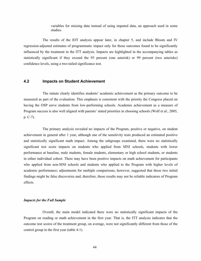
44
variables for missing data instead of using imputed data, an approach used in some studies.
The results of the IOT analysis appear later, in chapter 5, and include Bloom and IV regression-adjusted estimates of programmatic impact only for those outcomes found to be significantly influenced by the treatment in the ITT analysis. Impacts are highlighted in the accompanying tables as statistically significant if they exceed the 95 percent (one asterisk) or 99 percent (two asterisks) confidence levels, using a two-tailed significance test.
4.2 Impacts on Student Achievement
The statute clearly identifies students’ academic achievement as the primary outcome to be measured as part of the evaluation. This emphasis is consistent with the priority the Congress placed on having the OSP serve students from low-performing schools. Academic achievement as a measure of Program success is also well aligned with parents’ stated priorities in choosing schools (Wolf et al., 2005, p. C-7).
The primary analysis revealed no impacts of the Program, positive or negative, on student
achievement in general after 1 year, although one of the sensitivity tests produced an estimated positive and statistically significant math impact. Among the subgroups examined, there were no statistically significant test score impacts on students who applied from SINI schools, students with lower performance at baseline, male students, female students, elementary or high school students, or students in either individual cohort. There may have been positive impacts on math achievement for participants who applied from non-SINI schools and students who applied to the Program with higher levels of academic performance; adjustments for multiple comparisons, however, suggested that those two initial findings might be false discoveries and, therefore, those results may not be reliable indicators of Program effects.
Impacts for the Full Sample
Overall, the main model indicated there were no statistically significant impacts of the Program on reading or math achievement in the first year. That is, the ITT analysis indicates that the outcome test scores of the treatment group, on average, were not significantly different from those of the control group in the first year (table 4-1).
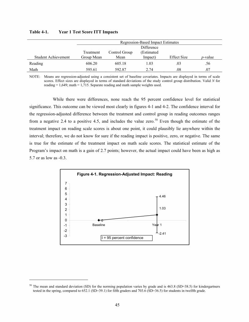
45
Table 4-1. Year 1 Test Score ITT Impacts Regression-Based Impact Estimates
Student Achievement Treatment
Group Mean Control Group
Mean
Difference (Estimated
Impact) Effect Size p-value Reading 606.20 605.18 1.03 .03 .56 Math 595.61 592.87 2.74 .08 .07
NOTE: Means are regression-adjusted using a consistent set of baseline covariates. Impacts are displayed in terms of scale scores. Effect sizes are displayed in terms of standard deviations of the study control group distribution. Valid N for reading = 1,649; math = 1,715. Separate reading and math sample weights used.
While there were differences, none reach the 95 percent confidence level for statistical
significance. This outcome can be viewed most clearly in figures 4-1 and 4-2. The confidence interval for the regression-adjusted difference between the treatment and control group in reading outcomes ranges from a negative 2.4 to a positive 4.5, and includes the value zero.58 Even though the estimate of the treatment impact on reading scale scores is about one point, it could plausibly lie anywhere within the interval; therefore, we do not know for sure if the reading impact is positive, zero, or negative. The same is true for the estimate of the treatment impact on math scale scores. The statistical estimate of the Program’s impact on math is a gain of 2.7 points; however, the actual impact could have been as high as 5.7 or as low as -0.3.
Figure 4-1. Regression-Adjusted Impact: Reading
0
1.03
-3-2-101234567
Baseline Year 1
I = 95 percent confidence
4.46
-2.41
58 The mean and standard deviation (SD) for the norming population varies by grade and is 463.8 (SD=38.5) for kindergartners
tested in the spring, compared to 652.1 (SD=39.1) for fifth graders and 703.6 (SD=36.5) for students in twelfth grade.
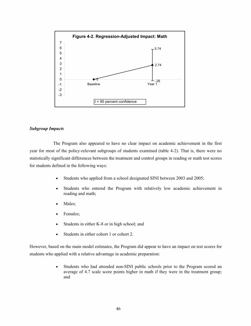
46
Figure 4-2. Regression-Adjusted Impact: Math
0
2.74
-3-2-101234567
Baseline Year 1
I = 95 percent confidence
5.74
-.26
Subgroup Impacts
The Program also appeared to have no clear impact on academic achievement in the first year for most of the policy-relevant subgroups of students examined (table 4-2). That is, there were no statistically significant differences between the treatment and control groups in reading or math test scores for students defined in the following ways:
• Students who applied from a school designated SINI between 2003 and 2005;
• Students who entered the Program with relatively low academic achievement in reading and math;
• Males;
• Females;
• Students in either K-8 or in high school; and
• Students in either cohort 1 or cohort 2.
However, based on the main model estimates, the Program did appear to have an impact on test scores for students who applied with a relative advantage in academic preparation:
• Students who had attended non-SINI public schools prior to the Program scored an average of 4.7 scale score points higher in math if they were in the treatment group; and
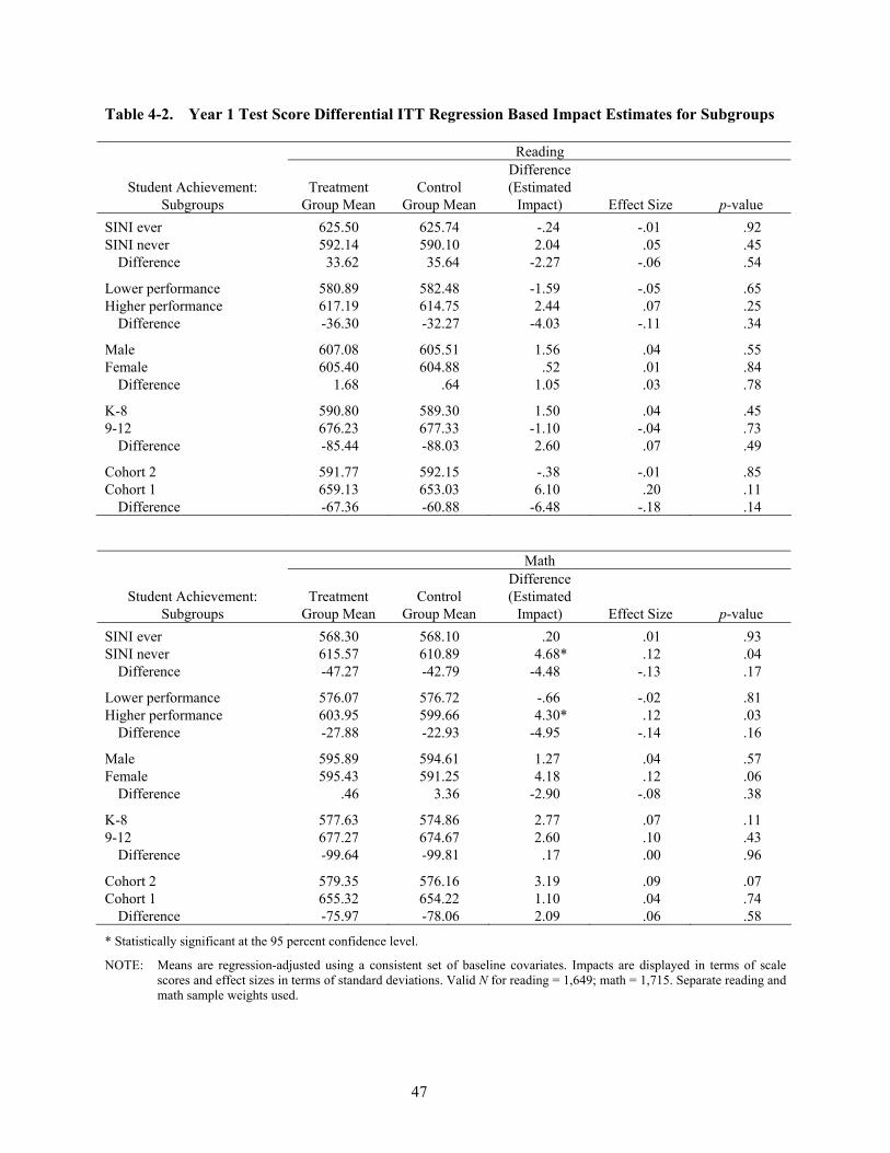
47
Table 4-2. Year 1 Test Score Differential ITT Regression Based Impact Estimates for Subgroups
Reading
Student Achievement: Subgroups
Treatment Group Mean
Control Group Mean
Difference (Estimated
Impact) Effect Size p-value SINI ever 625.50 625.74 -.24 -.01 .92 SINI never 592.14 590.10 2.04 .05 .45
Difference 33.62 35.64 -2.27 -.06 .54
Lower performance 580.89 582.48 -1.59 -.05 .65 Higher performance 617.19 614.75 2.44 .07 .25
Difference -36.30 -32.27 -4.03 -.11 .34
Male 607.08 605.51 1.56 .04 .55 Female 605.40 604.88 .52 .01 .84
Difference 1.68 .64 1.05 .03 .78
K-8 590.80 589.30 1.50 .04 .45 9-12 676.23 677.33 -1.10 -.04 .73
Difference -85.44 -88.03 2.60 .07 .49
Cohort 2 591.77 592.15 -.38 -.01 .85 Cohort 1 659.13 653.03 6.10 .20 .11
Difference -67.36 -60.88 -6.48 -.18 .14
Math
Student Achievement: Subgroups
Treatment Group Mean
Control Group Mean
Difference (Estimated
Impact) Effect Size p-value SINI ever 568.30 568.10 .20 .01 .93 SINI never 615.57 610.89 4.68* .12 .04
Difference -47.27 -42.79 -4.48 -.13 .17
Lower performance 576.07 576.72 -.66 -.02 .81 Higher performance 603.95 599.66 4.30* .12 .03
Difference -27.88 -22.93 -4.95 -.14 .16
Male 595.89 594.61 1.27 .04 .57 Female 595.43 591.25 4.18 .12 .06
Difference .46 3.36 -2.90 -.08 .38
K-8 577.63 574.86 2.77 .07 .11 9-12 677.27 674.67 2.60 .10 .43
Difference -99.64 -99.81 .17 .00 .96
Cohort 2 579.35 576.16 3.19 .09 .07 Cohort 1 655.32 654.22 1.10 .04 .74
Difference -75.97 -78.06 2.09 .06 .58
* Statistically significant at the 95 percent confidence level.
NOTE: Means are regression-adjusted using a consistent set of baseline covariates. Impacts are displayed in terms of scale scores and effect sizes in terms of standard deviations. Valid N for reading = 1,649; math = 1,715. Separate reading and math sample weights used.
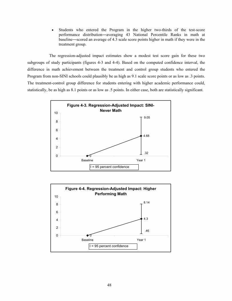
48
• Students who entered the Program in the higher two-thirds of the test-score performance distribution―averaging 43 National Percentile Ranks in math at baseline―scored an average of 4.3 scale score points higher in math if they were in the treatment group.
The regression-adjusted impact estimates show a modest test score gain for these two subgroups of study participants (figures 4-3 and 4-4). Based on the computed confidence interval, the difference in math achievement between the treatment and control group students who entered the Program from non-SINI schools could plausibly be as high as 9.1 scale score points or as low as .3 points. The treatment-control group difference for students entering with higher academic performance could, statistically, be as high as 8.1 points or as low as .5 points. In either case, both are statistically significant.
Figure 4-3. Regression-Adjusted Impact: SINI- Never Math
0
4.68
0
2
4
6
8
10
Baseline Year 1
I = 95 percent confidence i t l
9.05
.32
Figure 4-4. Regression-Adjusted Impact: Higher Performing Math
0
4.3
0
2
4
6
8
10
Baseline Year 1
I = 95 percent confidence i t l
8.14
.46
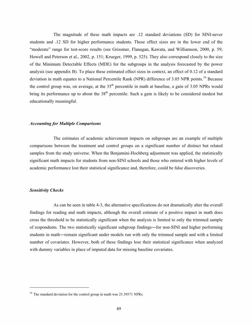
49
The magnitude of these math impacts are .12 standard deviations (SD) for SINI-never students and .12 SD for higher performance students. These effect sizes are in the lower end of the “moderate” range for test-score results (see Grissmer, Flanagan, Kawata, and Williamson, 2000, p. 59; Howell and Peterson et al., 2002, p. 151; Krueger, 1999, p. 525). They also correspond closely to the size of the Minimum Detectable Effects (MDE) for the subgroups in the analysis forecasted by the power analysis (see appendix B). To place these estimated effect sizes in context, an effect of 0.12 of a standard deviation in math equates to a National Percentile Rank (NPR) difference of 3.05 NPR points.59 Because the control group was, on average, at the 35th percentile in math at baseline, a gain of 3.05 NPRs would bring its performance up to about the 38th percentile. Such a gain is likely to be considered modest but educationally meaningful.
Accounting for Multiple Comparisons
The estimates of academic achievement impacts on subgroups are an example of multiple comparisons between the treatment and control groups on a significant number of distinct but related samples from the study universe. When the Benjamini-Hochberg adjustment was applied, the statistically significant math impacts for students from non-SINI schools and those who entered with higher levels of academic performance lost their statistical significance and, therefore, could be false discoveries.
Sensitivity Checks
As can be seen in table 4-3, the alternative specifications do not dramatically alter the overall findings for reading and math impacts, although the overall estimate of a positive impact in math does cross the threshold to be statistically significant when the analysis is limited to only the trimmed sample of respondents. The two statistically significant subgroup findings―for non-SINI and higher performing students in math―remain significant under models run with only the trimmed sample and with a limited number of covariates. However, both of these findings lose their statistical significance when analyzed with dummy variables in place of imputed data for missing baseline covariates.
59 The standard deviation for the control group in math was 25.39571 NPRs.
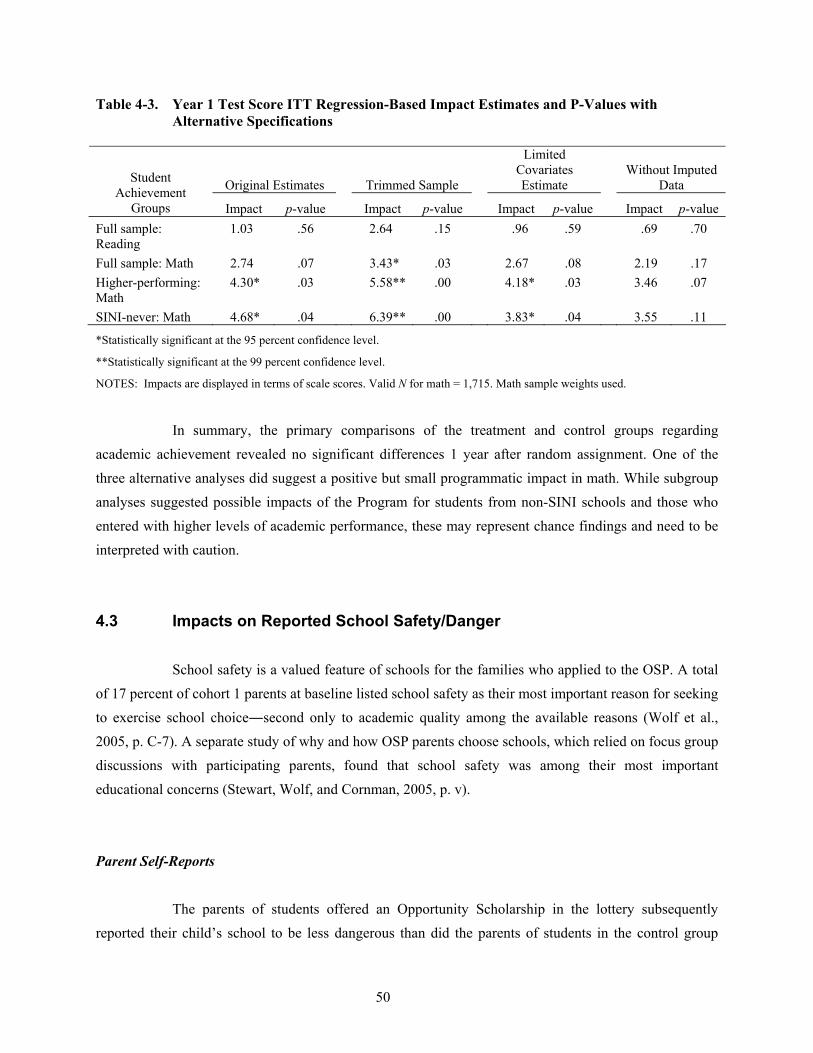
50
Table 4-3. Year 1 Test Score ITT Regression-Based Impact Estimates and P-Values with Alternative Specifications
Original Estimates Trimmed Sample
Limited Covariates Estimate
Without Imputed Data Student
Achievement Groups Impact p-value Impact p-value Impact p-value Impact p-value
Full sample: Reading
1.03 .56 2.64 .15 .96 .59 .69 .70
Full sample: Math 2.74 .07 3.43* .03 2.67 .08 2.19 .17 Higher-performing: Math
4.30* .03 5.58** .00 4.18* .03 3.46 .07
SINI-never: Math 4.68* .04 6.39** .00 3.83* .04 3.55 .11
*Statistically significant at the 95 percent confidence level.
**Statistically significant at the 99 percent confidence level.
NOTES: Impacts are displayed in terms of scale scores. Valid N for math = 1,715. Math sample weights used.
In summary, the primary comparisons of the treatment and control groups regarding
academic achievement revealed no significant differences 1 year after random assignment. One of the three alternative analyses did suggest a positive but small programmatic impact in math. While subgroup analyses suggested possible impacts of the Program for students from non-SINI schools and those who entered with higher levels of academic performance, these may represent chance findings and need to be interpreted with caution.
4.3 Impacts on Reported School Safety/Danger
School safety is a valued feature of schools for the families who applied to the OSP. A total of 17 percent of cohort 1 parents at baseline listed school safety as their most important reason for seeking to exercise school choice―second only to academic quality among the available reasons (Wolf et al., 2005, p. C-7). A separate study of why and how OSP parents choose schools, which relied on focus group discussions with participating parents, found that school safety was among their most important educational concerns (Stewart, Wolf, and Cornman, 2005, p. v).
Parent Self-Reports
The parents of students offered an Opportunity Scholarship in the lottery subsequently reported their child’s school to be less dangerous than did the parents of students in the control group
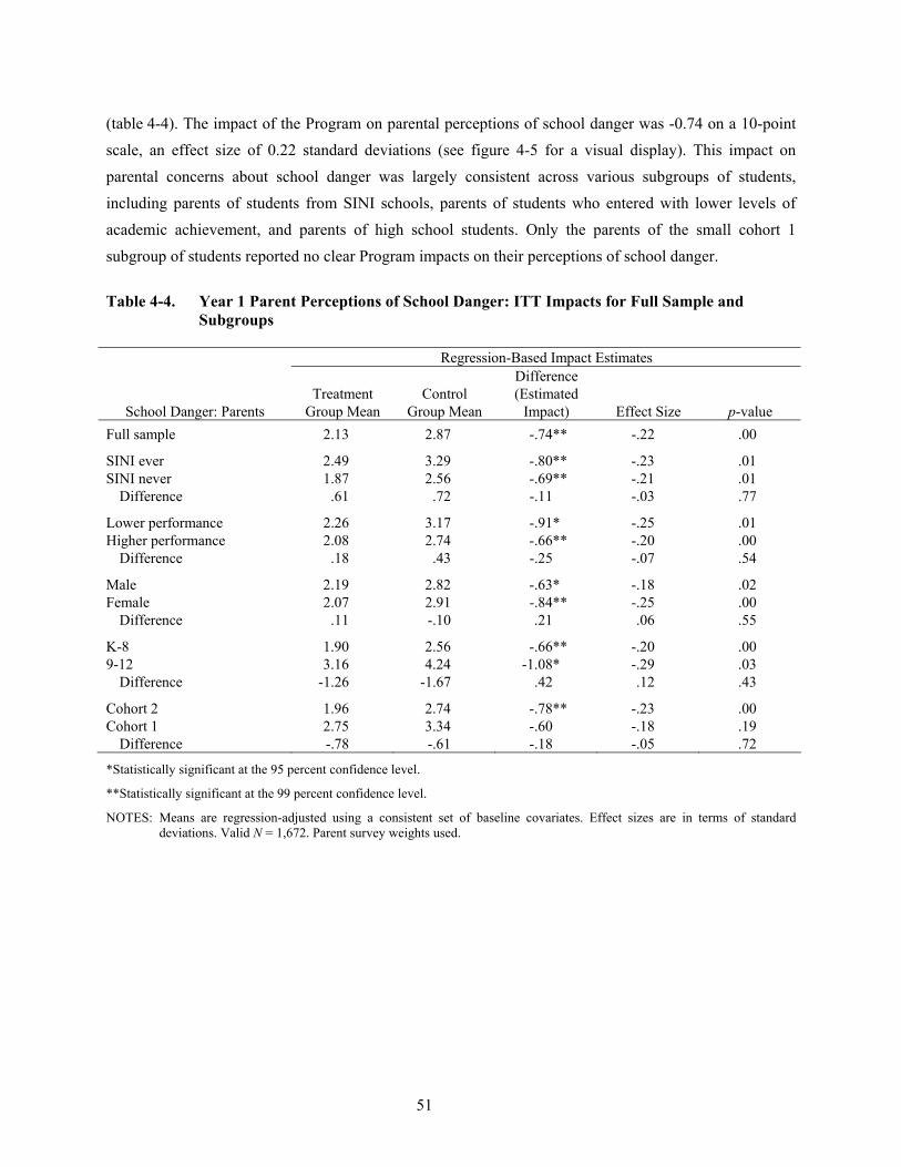
51
(table 4-4). The impact of the Program on parental perceptions of school danger was -0.74 on a 10-point scale, an effect size of 0.22 standard deviations (see figure 4-5 for a visual display). This impact on parental concerns about school danger was largely consistent across various subgroups of students, including parents of students from SINI schools, parents of students who entered with lower levels of academic achievement, and parents of high school students. Only the parents of the small cohort 1 subgroup of students reported no clear Program impacts on their perceptions of school danger.
Table 4-4. Year 1 Parent Perceptions of School Danger: ITT Impacts for Full Sample and
Subgroups
Regression-Based Impact Estimates
School Danger: Parents Treatment
Group Mean Control
Group Mean
Difference (Estimated
Impact) Effect Size p-value Full sample 2.13 2.87 -.74** -.22 .00
SINI ever 2.49 3.29 -.80** -.23 .01 SINI never 1.87 2.56 -.69** -.21 .01
Difference .61 .72 -.11 -.03 .77
Lower performance 2.26 3.17 -.91* -.25 .01 Higher performance 2.08 2.74 -.66** -.20 .00
Difference .18 .43 -.25 -.07 .54
Male 2.19 2.82 -.63* -.18 .02 Female 2.07 2.91 -.84** -.25 .00
Difference .11 -.10 .21 .06 .55
K-8 1.90 2.56 -.66** -.20 .00 9-12 3.16 4.24 -1.08* -.29 .03
Difference -1.26 -1.67 .42 .12 .43
Cohort 2 1.96 2.74 -.78** -.23 .00 Cohort 1 2.75 3.34 -.60 -.18 .19
Difference -.78 -.61 -.18 -.05 .72
*Statistically significant at the 95 percent confidence level.
**Statistically significant at the 99 percent confidence level.
NOTES: Means are regression-adjusted using a consistent set of baseline covariates. Effect sizes are in terms of standard deviations. Valid N = 1,672. Parent survey weights used.
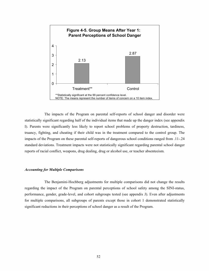
52
The impacts of the Program on parental self-reports of school danger and disorder were statistically significant regarding half of the individual items that made up the danger index (see appendix I). Parents were significantly less likely to report school problems of property destruction, tardiness, truancy, fighting, and cheating if their child was in the treatment compared to the control group. The impacts of the Program on these parental self-reports of dangerous school conditions ranged from .11-.24 standard deviations. Treatment impacts were not statistically significant regarding parental school danger reports of racial conflict, weapons, drug dealing, drug or alcohol use, or teacher absenteeism.
Accounting for Multiple Comparisons
The Benjamini-Hochberg adjustments for multiple comparisons did not change the results regarding the impact of the Program on parental perceptions of school safety among the SINI-status, performance, gender, grade-level, and cohort subgroups tested (see appendix J). Even after adjustments for multiple comparisons, all subgroups of parents except those in cohort 1 demonstrated statistically significant reductions in their perceptions of school danger as a result of the Program.
Figure 4-5. Group Means After Year 1: Parent Perceptions of School Danger
2.13
2.87
0
1
2
3
4
Treatment** Control**Statistically significant at the 99 percent confidence level.NOTE: The means represent the number of items of concern on a 10 item index.
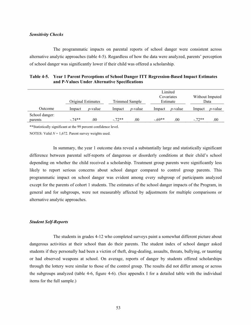
53
Sensitivity Checks
The programmatic impacts on parental reports of school danger were consistent across alternative analytic approaches (table 4-5). Regardless of how the data were analyzed, parents’ perception of school danger was significantly lower if their child was offered a scholarship.
Table 4-5. Year 1 Parent Perceptions of School Danger ITT Regression-Based Impact Estimates
and P-Values Under Alternative Specifications
Original Estimates Trimmed Sample
Limited Covariates Estimate
Without Imputed Data
Outcome Impact p-value Impact p-value Impact p-value Impact p-value School danger: parents -.74** .00 -.72** .00 -.69** .00 -.72** .00
**Statistically significant at the 99 percent confidence level.
NOTES: Valid N = 1,672. Parent survey weights used.
In summary, the year 1 outcome data reveal a substantially large and statistically significant
difference between parental self-reports of dangerous or disorderly conditions at their child’s school depending on whether the child received a scholarship. Treatment group parents were significantly less likely to report serious concerns about school danger compared to control group parents. This programmatic impact on school danger was evident among every subgroup of participants analyzed except for the parents of cohort 1 students. The estimates of the school danger impacts of the Program, in general and for subgroups, were not measurably affected by adjustments for multiple comparisons or alternative analytic approaches.
Student Self-Reports
The students in grades 4-12 who completed surveys paint a somewhat different picture about dangerous activities at their school than do their parents. The student index of school danger asked students if they personally had been a victim of theft, drug-dealing, assaults, threats, bullying, or taunting or had observed weapons at school. On average, reports of danger by students offered scholarships through the lottery were similar to those of the control group. The results did not differ among or across the subgroups analyzed (table 4-6, figure 4-6). (See appendix I for a detailed table with the individual items for the full sample.)

54
Table 4-6. Year 1 Student Perceptions of School Danger: ITT Impacts for Full Sample and Subgroups
Regression-Based Impact Estimates
School Danger: Students Treatment
Group Mean Control
Group Mean
Difference (Estimated
Impact) Effect Size p-value Full sample 1.89 2.09 -.21 -.11 .22
SINI ever 2.02 2.25 -.24 -.12 .30 SINI never 1.80 1.98 -.18 -.10 .44
Difference .22 .27 -.05 -.03 .86
Lower performance 2.07 2.13 -.06 -.03 .84 Higher performance -1.82 2.08 -.26 -.14 .19
Difference .25 .05 .20 .10 .57
Male 2.09 2.40 -.31 -.15 .21 Female 1.69 1.80 -.11 -.06 .62
Difference .40 .60 -.20 -.10 .53
4-8 1.99 2.18 -.19 -.10 .34 9-12 1.44 1.73 -.29 -.16 .19
Difference .55 .45 .10 .05 .73
Cohort 2 1.96 2.19 -.24 -.12 .25 Cohort 1 1.65 1.76 -.10 -.06 .66
Difference .30 .44 -.13 -.07 .66
NOTES: Means are regression-adjusted using a consistent set of baseline covariates. Effect sizes are in terms of standard deviations. Valid N = 968. Student survey weights used. Survey given to students in grades 4-12.
Figure 4-6. Group Means After Year 1: Student Perceptions of School Danger
1.89 2.09
0
1
2
3
4
Treatment Control
NOTE: The means represent the number of incidents on an 8-item index.
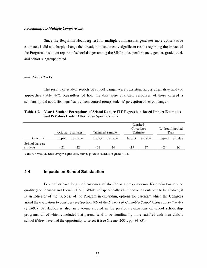
55
Accounting for Multiple Comparisons
Since the Benjamini-Hochberg test for multiple comparisons generates more conservative estimates, it did not sharply change the already non-statistically significant results regarding the impact of the Program on student reports of school danger among the SINI-status, performance, gender, grade-level, and cohort subgroups tested.
Sensitivity Checks
The results of student reports of school danger were consistent across alternative analytic approaches (table 4-7). Regardless of how the data were analyzed, responses of those offered a scholarship did not differ significantly from control group students’ perception of school danger.
Table 4-7. Year 1 Student Perceptions of School Danger ITT Regression-Based Impact Estimates
and P-Values Under Alternative Specifications
Original Estimates Trimmed Sample
Limited Covariates Estimate
Without Imputed Data
Outcome Impact p-value Impact p-value Impact p-value Impact p-value School danger: students -.21 .22 -.21 .24 -.19 .27 -.24 .16
Valid N = 968. Student survey weights used. Survey given to students in grades 4-12.
4.4 Impacts on School Satisfaction
Economists have long used customer satisfaction as a proxy measure for product or service quality (see Johnson and Fornell, 1991). While not specifically identified as an outcome to be studied, it is an indicator of the “success of the Program in expanding options for parents,” which the Congress asked the evaluation to consider (see Section 309 of the District of Columbia School Choice Incentive Act of 2003). Satisfaction is also an outcome studied in the previous evaluations of school scholarship programs, all of which concluded that parents tend to be significantly more satisfied with their child’s school if they have had the opportunity to select it (see Greene, 2001, pp. 84-85).
56
Parent Self-Reports
Seven months after the start of their experience with the OSP, parents are more satisfied with their child’s school if they were offered a scholarship (table 4-8, figures 4-7 through 4-9). Three different measures of parent satisfaction all show large statistically significant positive impacts of the Program on parental evaluations of their child’s school:
• A total of 74 percent of treatment parents assigned their child’s school a grade of A or
B compared with 55 percent of control parents―a difference of 19 percentage points.
• On a scale of A-F, the average grade assigned to the school by parents of treatment students was nearly one-half grade higher than that of control parents―a statistically significant difference.
• Parents of students in the treatment group scored an average of more than three points higher than parents of students in the control group on the school satisfaction index―again a statistically significant programmatic impact.
The magnitude of these positive OSP impacts on parental satisfaction (the effect sizes) ranged from .37 to .38 standard deviations. The parent satisfaction scale comprised 12 separate items asking how dissatisfied or satisfied they were with a variety of characteristics of their child’s school including location, academics, teachers, facilities, safety, communication, parental support, etc. Each of the 12 items was rated on a 4-point scale. Using Item Response Theory (IRT) techniques, a summary scale was constructed with a range of .55 to 35.54. Positive statistically significant treatment impacts were observed for each of the 12 individual components of the parental school satisfaction scale (see appendix I for a detailed table with the individual items).
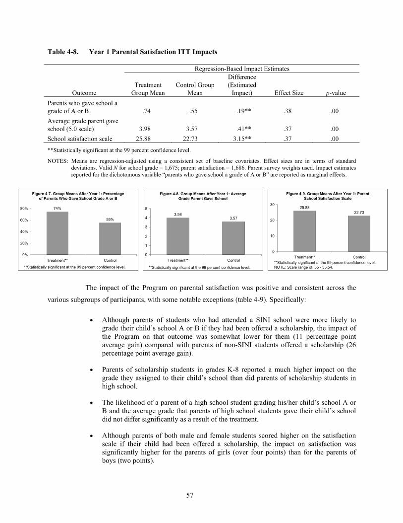
57
Table 4-8. Year 1 Parental Satisfaction ITT Impacts
Regression-Based Impact Estimates
Outcome Treatment
Group Mean Control Group
Mean
Difference (Estimated
Impact) Effect Size p-value Parents who gave school a grade of A or B .74 .55 .19** .38 .00 Average grade parent gave school (5.0 scale) 3.98 3.57 .41** .37 .00 School satisfaction scale 25.88 22.73 3.15** .37 .00
**Statistically significant at the 99 percent confidence level.
NOTES: Means are regression-adjusted using a consistent set of baseline covariates. Effect sizes are in terms of standard deviations. Valid N for school grade = 1,675; parent satisfaction = 1,686. Parent survey weights used. Impact estimates reported for the dichotomous variable “parents who gave school a grade of A or B” are reported as marginal effects.
The impact of the Program on parental satisfaction was positive and consistent across the various subgroups of participants, with some notable exceptions (table 4-9). Specifically:
• Although parents of students who had attended a SINI school were more likely to
grade their child’s school A or B if they had been offered a scholarship, the impact of the Program on that outcome was somewhat lower for them (11 percentage point average gain) compared with parents of non-SINI students offered a scholarship (26 percentage point average gain).
• Parents of scholarship students in grades K-8 reported a much higher impact on the grade they assigned to their child’s school than did parents of scholarship students in high school.
• The likelihood of a parent of a high school student grading his/her child’s school A or B and the average grade that parents of high school students gave their child’s school did not differ significantly as a result of the treatment.
• Although parents of both male and female students scored higher on the satisfaction scale if their child had been offered a scholarship, the impact on satisfaction was significantly higher for the parents of girls (over four points) than for the parents of boys (two points).
Figure 4-7. Group Means After Year 1: Percentage of Parents Who Gave School Grade A or B
74%
55%
0%
20%
40%
60%
80%
Treatment** Control
**Statistically significant at the 99 percent confidence level.
Figure 4-8. Group Means After Year 1: Average Grade Parent Gave School
3.983.57
0
1
2
3
4
5
Treatment** Control
**Statistically significant at the 99 percent confidence level.
Figure 4-9. Group Means After Year 1: Parent School Satisfaction Scale
25.8822.73
0
10
20
30
Treatment** Control**Statistically significant at the 99 percent confidence level.NOTE: Scale range of .55 - 35.54.
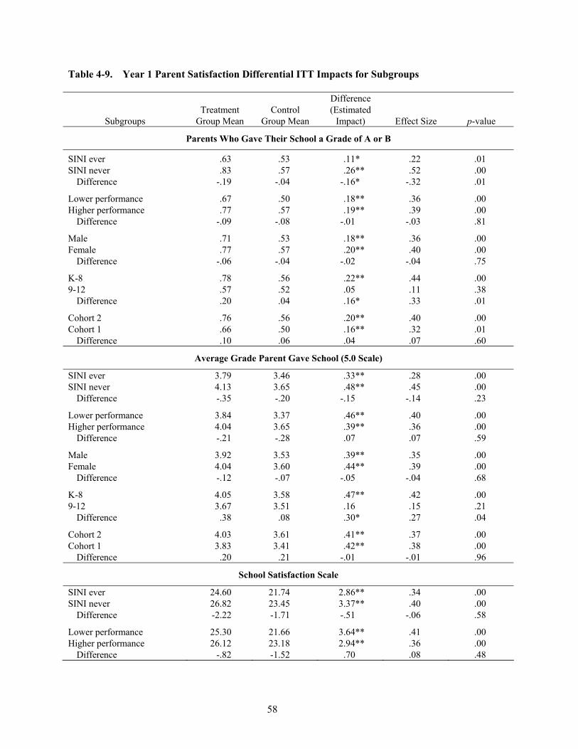
58
Table 4-9. Year 1 Parent Satisfaction Differential ITT Impacts for Subgroups
Subgroups Treatment
Group Mean Control
Group Mean
Difference (Estimated
Impact) Effect Size p-value
Parents Who Gave Their School a Grade of A or B
SINI ever .63 .53 .11* .22 .01 SINI never .83 .57 .26** .52 .00
Difference -.19 -.04 -.16* -.32 .01
Lower performance .67 .50 .18** .36 .00 Higher performance .77 .57 .19** .39 .00
Difference -.09 -.08 -.01 -.03 .81
Male .71 .53 .18** .36 .00 Female .77 .57 .20** .40 .00
Difference -.06 -.04 -.02 -.04 .75
K-8 .78 .56 .22** .44 .00 9-12 .57 .52 .05 .11 .38
Difference .20 .04 .16* .33 .01
Cohort 2 .76 .56 .20** .40 .00 Cohort 1 .66 .50 .16** .32 .01
Difference .10 .06 .04 .07 .60
Average Grade Parent Gave School (5.0 Scale)
SINI ever 3.79 3.46 .33** .28 .00 SINI never 4.13 3.65 .48** .45 .00
Difference -.35 -.20 -.15 -.14 .23
Lower performance 3.84 3.37 .46** .40 .00 Higher performance 4.04 3.65 .39** .36 .00
Difference -.21 -.28 .07 .07 .59
Male 3.92 3.53 .39** .35 .00 Female 4.04 3.60 .44** .39 .00
Difference -.12 -.07 -.05 -.04 .68
K-8 4.05 3.58 .47** .42 .00 9-12 3.67 3.51 .16 .15 .21
Difference .38 .08 .30* .27 .04
Cohort 2 4.03 3.61 .41** .37 .00 Cohort 1 3.83 3.41 .42** .38 .00
Difference .20 .21 -.01 -.01 .96
School Satisfaction Scale
SINI ever 24.60 21.74 2.86** .34 .00 SINI never 26.82 23.45 3.37** .40 .00
Difference -2.22 -1.71 -.51 -.06 .58
Lower performance 25.30 21.66 3.64** .41 .00 Higher performance 26.12 23.18 2.94** .36 .00
Difference -.82 -1.52 .70 .08 .48
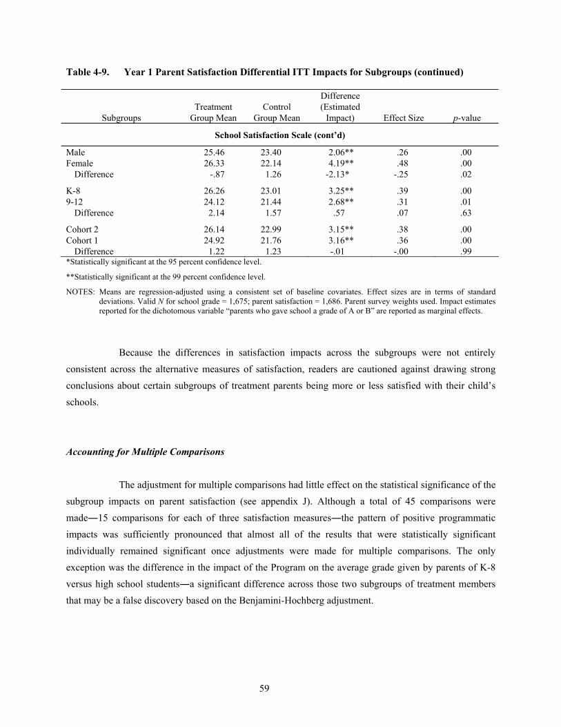
59
Table 4-9. Year 1 Parent Satisfaction Differential ITT Impacts for Subgroups (continued)
Subgroups Treatment
Group Mean Control
Group Mean
Difference (Estimated
Impact) Effect Size p-value
School Satisfaction Scale (cont’d)
Male 25.46 23.40 2.06** .26 .00 Female 26.33 22.14 4.19** .48 .00
Difference -.87 1.26 -2.13* -.25 .02
K-8 26.26 23.01 3.25** .39 .00 9-12 24.12 21.44 2.68** .31 .01
Difference 2.14 1.57 .57 .07 .63
Cohort 2 26.14 22.99 3.15** .38 .00 Cohort 1 24.92 21.76 3.16** .36 .00
Difference 1.22 1.23 -.01 -.00 .99 *Statistically significant at the 95 percent confidence level.
**Statistically significant at the 99 percent confidence level.
NOTES: Means are regression-adjusted using a consistent set of baseline covariates. Effect sizes are in terms of standard deviations. Valid N for school grade = 1,675; parent satisfaction = 1,686. Parent survey weights used. Impact estimates reported for the dichotomous variable “parents who gave school a grade of A or B” are reported as marginal effects.
Because the differences in satisfaction impacts across the subgroups were not entirely
consistent across the alternative measures of satisfaction, readers are cautioned against drawing strong conclusions about certain subgroups of treatment parents being more or less satisfied with their child’s schools.
Accounting for Multiple Comparisons
The adjustment for multiple comparisons had little effect on the statistical significance of the subgroup impacts on parent satisfaction (see appendix J). Although a total of 45 comparisons were made―15 comparisons for each of three satisfaction measures―the pattern of positive programmatic impacts was sufficiently pronounced that almost all of the results that were statistically significant individually remained significant once adjustments were made for multiple comparisons. The only exception was the difference in the impact of the Program on the average grade given by parents of K-8 versus high school students―a significant difference across those two subgroups of treatment members that may be a false discovery based on the Benjamini-Hochberg adjustment.
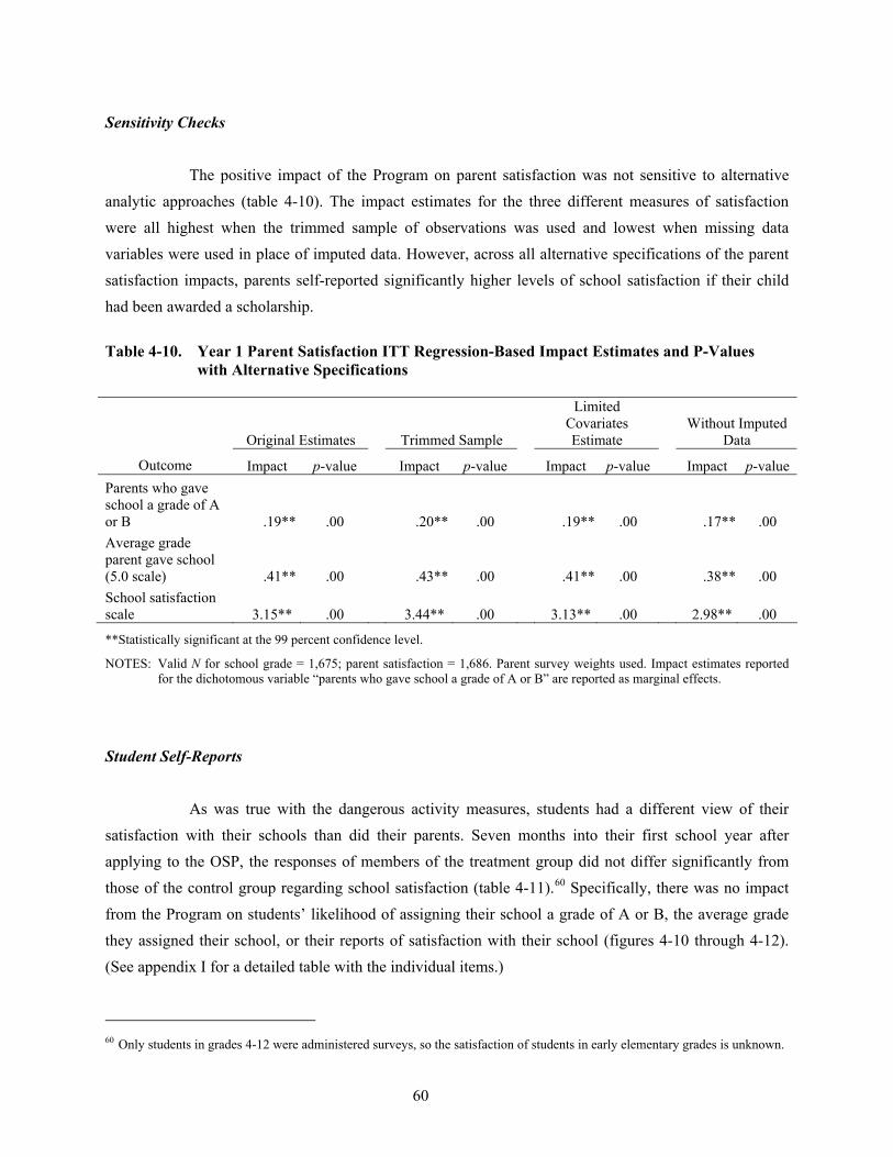
60
Sensitivity Checks
The positive impact of the Program on parent satisfaction was not sensitive to alternative analytic approaches (table 4-10). The impact estimates for the three different measures of satisfaction were all highest when the trimmed sample of observations was used and lowest when missing data variables were used in place of imputed data. However, across all alternative specifications of the parent satisfaction impacts, parents self-reported significantly higher levels of school satisfaction if their child had been awarded a scholarship.
Table 4-10. Year 1 Parent Satisfaction ITT Regression-Based Impact Estimates and P-Values
with Alternative Specifications
Original Estimates Trimmed Sample
Limited Covariates Estimate
Without Imputed Data
Outcome Impact p-value Impact p-value Impact p-value Impact p-value Parents who gave school a grade of A or B .19** .00 .20** .00 .19** .00 .17** .00 Average grade parent gave school (5.0 scale) .41** .00 .43** .00 .41** .00 .38** .00 School satisfaction scale 3.15** .00 3.44** .00 3.13** .00 2.98** .00
**Statistically significant at the 99 percent confidence level.
NOTES: Valid N for school grade = 1,675; parent satisfaction = 1,686. Parent survey weights used. Impact estimates reported for the dichotomous variable “parents who gave school a grade of A or B” are reported as marginal effects.
Student Self-Reports
As was true with the dangerous activity measures, students had a different view of their satisfaction with their schools than did their parents. Seven months into their first school year after applying to the OSP, the responses of members of the treatment group did not differ significantly from those of the control group regarding school satisfaction (table 4-11).60 Specifically, there was no impact from the Program on students’ likelihood of assigning their school a grade of A or B, the average grade they assigned their school, or their reports of satisfaction with their school (figures 4-10 through 4-12). (See appendix I for a detailed table with the individual items.)
60 Only students in grades 4-12 were administered surveys, so the satisfaction of students in early elementary grades is unknown.

61
Table 4-11. Year 1 Student Satisfaction ITT Impacts
Outcome Treatment
Group Mean Control
Group Mean
Difference (Estimated
Impact) Effect Size p-value Students who gave school a grade of A or B
.70 .72 -.01 -.03 .74
Average grade student gave school (5.0 scale)
3.99 3.99 .00 .00 .99
School satisfaction scale 33.74 33.56 .38 .06 .48
NOTES: Means are regression-adjusted using a consistent set of baseline covariates. Effect sizes are in terms of standard deviations. Valid N for school grade = 901; student satisfaction = 983. Student survey weights used. Impact estimates reported for the dichotomous variable “students who gave school a grade of A or B” are reported as marginal effects. Survey given to students in grades 4-12.
There were some differences across subgroups of students, however. In particular, there were negative impacts on satisfaction for students from SINI schools and for students who entered the Program with relative academic disadvantages (table 4-12):
• Among students from SINI schools, those awarded scholarships were more likely to
grade their school poorly than were those in the control group. In contrast, among students from non-SINI schools, those awarded scholarships were more likely to grade their school highly than were those in the control group. Neither subgroup impact was statistically significant; however, the difference in the treatment impact between students from SINI and non-SINI schools was itself statistically significant.
• Among students who applied to the Program with lower academic achievement, those awarded a scholarship were more likely to grade their school poorly than were those in the control group. This subgroup impact was statistically significant. The difference in the impact on satisfaction for lower achievement students versus higher achievement students also was itself statistically significant.
Figure 4-10. Group Means After Year 1: Percentage of Students Who Gave School Grade A or B
70% 72%
0%
20%
40%
60%
80%
Treatment Control
Figure 4-11. Group Means After Year 1: Average Grade Student Gave School
3.99 3.99
0
1
2
3
4
5
Treatment Control
Figure 4-12. Group Means After Year 1: Student School Satisfaction Scale Rating
33.74 33.56
8
18
28
38
Treatment Control
NOTE: Scale range of 8.44 - 46.45.
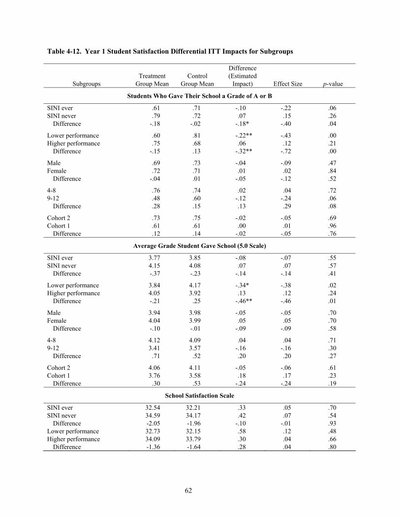
62
Table 4-12. Year 1 Student Satisfaction Differential ITT Impacts for Subgroups
Subgroups Treatment
Group Mean Control
Group Mean
Difference (Estimated
Impact) Effect Size p-value
Students Who Gave Their School a Grade of A or B
SINI ever .61 .71 -.10 -.22 .06 SINI never .79 .72 .07 .15 .26
Difference -.18 -.02 -.18* -.40 .04
Lower performance .60 .81 -.22** -.43 .00 Higher performance .75 .68 .06 .12 .21
Difference -.15 .13 -.32** -.72 .00
Male .69 .73 -.04 -.09 .47 Female .72 .71 .01 .02 .84
Difference -.04 .01 -.05 -.12 .52
4-8 .76 .74 .02 .04 .72 9-12 .48 .60 -.12 -.24 .06
Difference .28 .15 .13 .29 .08
Cohort 2 .73 .75 -.02 -.05 .69 Cohort 1 .61 .61 .00 .01 .96
Difference .12 .14 -.02 -.05 .76
Average Grade Student Gave School (5.0 Scale)
SINI ever 3.77 3.85 -.08 -.07 .55 SINI never 4.15 4.08 .07 .07 .57
Difference -.37 -.23 -.14 -.14 .41
Lower performance 3.84 4.17 -.34* -.38 .02 Higher performance 4.05 3.92 .13 .12 .24
Difference -.21 .25 -.46** -.46 .01
Male 3.94 3.98 -.05 -.05 .70 Female 4.04 3.99 .05 .05 .70
Difference -.10 -.01 -.09 -.09 .58
4-8 4.12 4.09 .04 .04 .71 9-12 3.41 3.57 -.16 -.16 .30
Difference .71 .52 .20 .20 .27
Cohort 2 4.06 4.11 -.05 -.06 .61 Cohort 1 3.76 3.58 .18 .17 .23
Difference .30 .53 -.24 -.24 .19
School Satisfaction Scale
SINI ever 32.54 32.21 .33 .05 .70 SINI never 34.59 34.17 .42 .07 .54
Difference -2.05 -1.96 -.10 -.01 .93 Lower performance 32.73 32.15 .58 .12 .48 Higher performance 34.09 33.79 .30 .04 .66
Difference -1.36 -1.64 .28 .04 .80
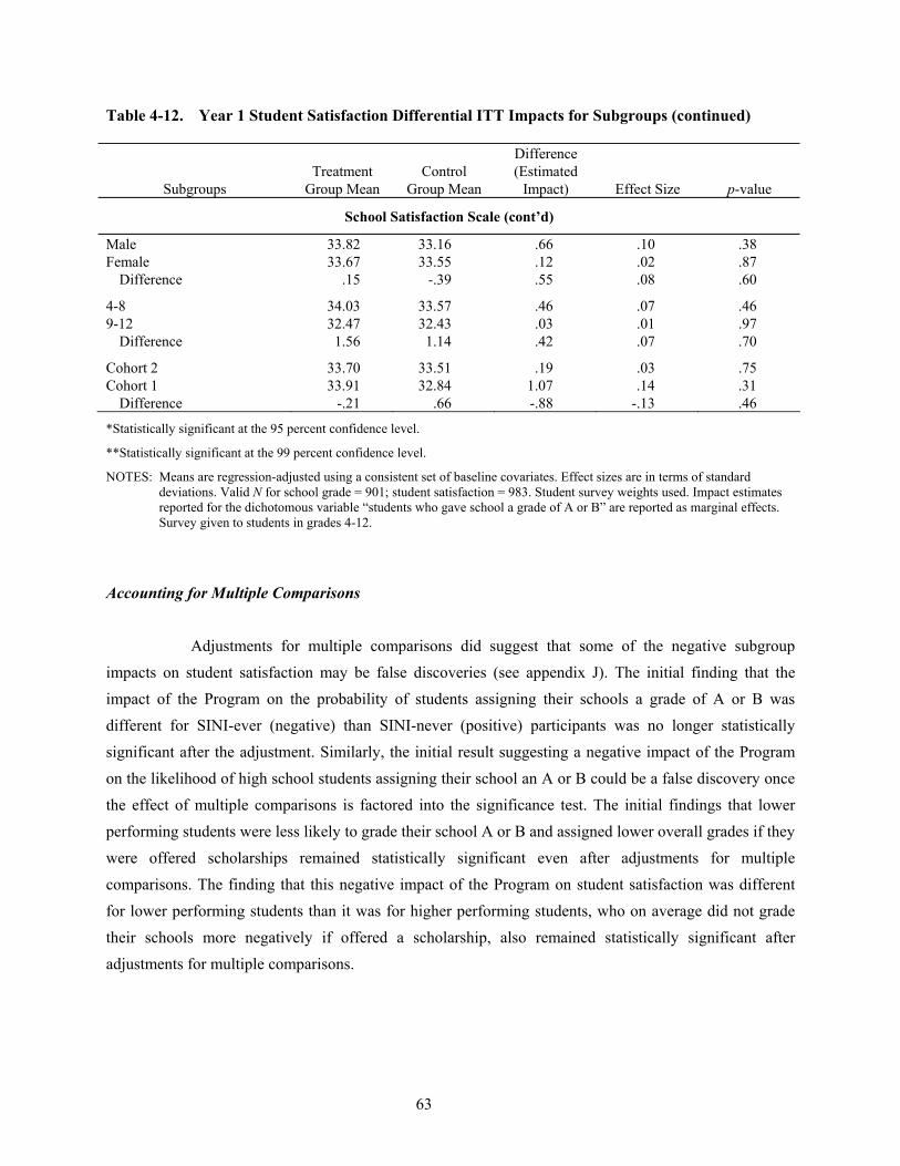
63
Table 4-12. Year 1 Student Satisfaction Differential ITT Impacts for Subgroups (continued)
Subgroups Treatment
Group Mean Control
Group Mean
Difference (Estimated
Impact) Effect Size p-value
School Satisfaction Scale (cont’d)
Male 33.82 33.16 .66 .10 .38 Female 33.67 33.55 .12 .02 .87
Difference .15 -.39 .55 .08 .60
4-8 34.03 33.57 .46 .07 .46 9-12 32.47 32.43 .03 .01 .97
Difference 1.56 1.14 .42 .07 .70
Cohort 2 33.70 33.51 .19 .03 .75 Cohort 1 33.91 32.84 1.07 .14 .31
Difference -.21 .66 -.88 -.13 .46
*Statistically significant at the 95 percent confidence level.
**Statistically significant at the 99 percent confidence level.
NOTES: Means are regression-adjusted using a consistent set of baseline covariates. Effect sizes are in terms of standard deviations. Valid N for school grade = 901; student satisfaction = 983. Student survey weights used. Impact estimates reported for the dichotomous variable “students who gave school a grade of A or B” are reported as marginal effects. Survey given to students in grades 4-12.
Accounting for Multiple Comparisons
Adjustments for multiple comparisons did suggest that some of the negative subgroup impacts on student satisfaction may be false discoveries (see appendix J). The initial finding that the impact of the Program on the probability of students assigning their schools a grade of A or B was different for SINI-ever (negative) than SINI-never (positive) participants was no longer statistically significant after the adjustment. Similarly, the initial result suggesting a negative impact of the Program on the likelihood of high school students assigning their school an A or B could be a false discovery once the effect of multiple comparisons is factored into the significance test. The initial findings that lower performing students were less likely to grade their school A or B and assigned lower overall grades if they were offered scholarships remained statistically significant even after adjustments for multiple comparisons. The finding that this negative impact of the Program on student satisfaction was different for lower performing students than it was for higher performing students, who on average did not grade their schools more negatively if offered a scholarship, also remained statistically significant after adjustments for multiple comparisons.

64
Sensitivity Checks
The main findings of no programmatic impact on overall student self-reports of satisfaction were consistent across the three alternative methodological approaches (table 4-13). There are no differences in the average student satisfaction levels of the overall treatment and control group after 1 year regardless of the satisfaction measure or analytic method used.
Table 4-13. Year 1 Student Satisfaction ITT Regression-Based Impact Estimates and P-Values with
Alternative Specifications
Original Estimates Trimmed Sample
Limited Covariates Estimate
Without Imputed Data
Outcome Impact p-value Impact p-value Impact p-value Impact p-value Students who gave school a grade of A or B -.01 .74 .01 .86 -.01 .74 -.02 .64 Average grade student gave school (5.0 scale) .00 .99 .04 .63 -.00 .97 .01 .92 School satisfaction scale .38 .48 .49 .37 .27 .62 .42 .43
NOTES: Valid N for school grade = 901; student satisfaction = 983. Student survey weights used. Impact estimates reported for the dichotomous variable “students who gave school a grade of A or B” are reported as marginal effects. Survey given to students in grades 4-12.
4.5 Summary of Experimental Impacts
One year after the students of cohort 1 and cohort 2 applied to the OSP and 7 months after they began their post-randomization educational experiences, those in the treatment group appear to be performing in mathematics and reading at a level comparable to the control group. The primary method of analysis and two of the three alternative methods indicated no statistically significant achievement gains attributable to the Program. The remaining alternative method, using the trimmed response sample, suggested an overall treatment impact of 3.4 scale score points in math that was statistically significant. Two subgroups of study participants―students who were non-SINI applicants and students who were higher performing when they applied―may have benefited from the Program in terms of their math achievement; however, adjustments that account for the fact that these two positive findings emerged from multiple comparisons suggest that they might be false discoveries, so they should be interpreted with caution.
65
The data indicate that parents are much more satisfied with their child’s school and view it as safer in many ways if they were offered an Opportunity Scholarship. These parent satisfaction impacts are positive, large, and consistent across almost all subgroups and not sensitive to adjustments for multiple comparisons or alternative analytic approaches. However, the Program had no impact overall on students’ views of school safety and satisfaction; students who entered the Program with lower academic achievement graded their schools lower if they had been offered a scholarship.
These results can be placed in the context of other RCTs of scholarship programs for low-
income students, which suggest no consistent pattern of academic achievement impacts for the first year of program participation. Among such evaluations of four privately funded scholarship programs, one study of the Charlotte, North Carolina, program clearly found statistically significant overall impacts on math and reading for the first year, while one of three analyses of the New York City program found overall impacts on math achievement (Barnard et al., 2003; Greene, 2000). When African-Americans are considered separately―a group that makes up nearly 90 percent of the OSP impact study sample―two of three analyses of the New York City program suggest there were achievement gains in math for African-American students in some grade levels (Barnard et al., 2003; Mayer et al., 2002), but studies of the Dayton, Ohio, and earlier District of Columbia programs found no impacts for this group until students were in the program for 2 years (Howell et al., 2002). In contrast, all of the RCTs that measured parent satisfaction and perceptions of school safety found positive impacts similar to those demonstrated by the OSP the first year (Greene, 2000; Howell and Peterson et al., 2002;).

67
5. The Effects of OSP Scholarship Use and Private Schooling
The previous chapter described the experimental impacts from the Program, observed about a year after students applied to it. Those results provide initial answers to the question: “What happened to qualified applicants who were offered Opportunity Scholarships?” However, as outlined elsewhere in the report, there are related questions about Program effects that are also of interest to policymakers. The two most important are addressed here, and not in the prior chapter, because they deviate to different extents from the randomized trial that grounds the rigor of the evaluation (see chapter 3 for a discussion of methodology and appendix G for the specific statistical techniques and models used here). This chapter presents information on the estimated effects of (1) “using” a scholarship to attend a participating private school (what we call the impact on the treated or IOT) and (2) attending a private school, regardless of scholarship use, with the latter based on statistical techniques that make the estimate the best proxy for, but not, an experimental impact. Each section starts off with the context and rationale for the analysis and then describes the analysis results.
5.1 Effect of Using a Scholarship
The intention-to-treat (ITT) impacts discussed in chapter 4 describe the average impacts of the OSP on the entire group of students who were selected randomly in the lottery to receive the offer of a scholarship. However, about one-fifth of these treatment students did not use their scholarship the first year. Since the rate of treatment nonuse will vary over time and across scholarship programs, policymakers have expressed an interest in understanding the impact of the OSP on the students who actually used their scholarships to attend participating private schools (the IOT estimate).
Interpreting the Impacts on the Treated (IOT)
As described in chapter 3, estimating the impact of using an OSP scholarship involves “netting out” from the ITT results two groups of students: (1) the 20 percent who received but failed to take up the scholarship offer and who, therefore, presumably, had zero impact from the Program, and (2) the hypothesized 4 percent who never received a scholarship offer but who, by virtue of having a sibling
68
with an OSP scholarship, wound up in a participating private school. Both adjustments have the effect of increasing the size of any observed statistically significant ITT impacts of the Program.
These statistical procedures for estimating the effects of scholarship usage do not change the
treatment- or control-group status of any participants. Bloom adjustments draw upon the existing patterns in the experimental data to generate unbiased estimates of what the programmatic effects were for the treatment members who actually used their scholarship compared with the counterfactual provided by the control group. The number of “noncompliers”―treatment “decliners” and control “crossovers”―factor into these statistical estimates, but treatment decliners are never mixed with the control group nor are control crossovers considered treatment-group members for purposes of these calculations. The findings from the purely experimental ITT analysis are simply taken from the entire treatment group and rescaled across the subgroup of treatment users (i.e., Bloom adjusted). The double-Bloom adjustments presented here merely further adjust mathematically for the somewhat anomalous cases of Program-induced control crossovers that emerged in this particular RCT.
When estimating the impact of scholarship use (IOT), the ITT results serve an important
screening function. If an impact is not statistically significant in the ITT stage of the analysis, it makes little sense to consider what its IOT effects might be. Experimental impacts that fail to attain an acceptable level of statistical significance are considered to be impacts of zero; that is, an impact of zero rescaled by way of a Bloom or double-Bloom adjustment will remain zero.
In short, a finding must emerge as statistically significant in the experimental evaluation of
the impact of the scholarship offer in order for there to be any hope of that finding shedding light on the question of the effects of actually using a scholarship if offered one. As a result, we only present IOT effect estimates for Program impacts found to be statistically significant in the ITT analysis reported in chapter 4. The adjustments for multiple comparisons and sensitivity test results reported for the statistically significant impacts in chapter 4 apply directly to the rescaled IOT results presented here. We use the same full sample of year 1 outcome observations used in the ITT analysis for the subsequent analyses here.
IOT Effects on Achievement
The ITT analysis presented in chapter 4 found no evidence of an overall impact of the first year of the Program on student test scores in either reading or math. The effect of using a scholarship on these outcomes is similar.
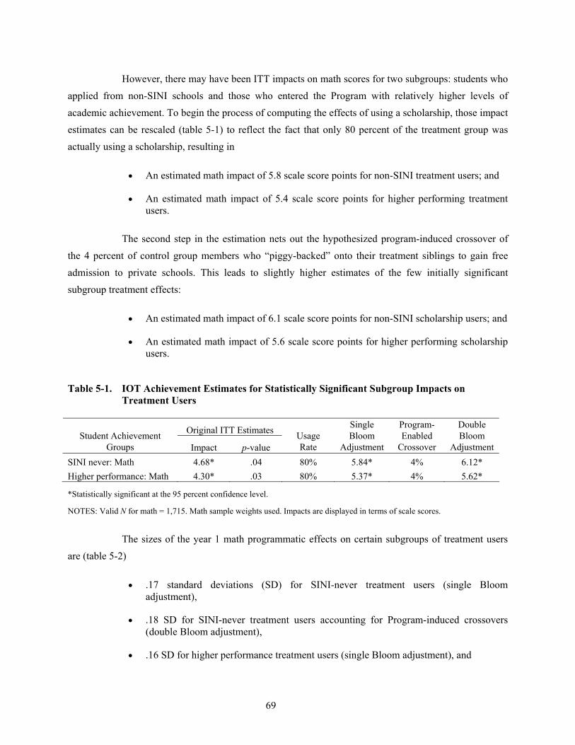
69
However, there may have been ITT impacts on math scores for two subgroups: students who applied from non-SINI schools and those who entered the Program with relatively higher levels of academic achievement. To begin the process of computing the effects of using a scholarship, those impact estimates can be rescaled (table 5-1) to reflect the fact that only 80 percent of the treatment group was actually using a scholarship, resulting in
• An estimated math impact of 5.8 scale score points for non-SINI treatment users; and
• An estimated math impact of 5.4 scale score points for higher performing treatment users.
The second step in the estimation nets out the hypothesized program-induced crossover of the 4 percent of control group members who “piggy-backed” onto their treatment siblings to gain free admission to private schools. This leads to slightly higher estimates of the few initially significant subgroup treatment effects:
• An estimated math impact of 6.1 scale score points for non-SINI scholarship users; and
• An estimated math impact of 5.6 scale score points for higher performing scholarship users.
Table 5-1. IOT Achievement Estimates for Statistically Significant Subgroup Impacts on
Treatment Users
Original ITT Estimates Student Achievement Groups Impact p-value
Usage Rate
Single Bloom
Adjustment
Program-Enabled
Crossover
Double Bloom
Adjustment SINI never: Math 4.68* .04 80% 5.84* 4% 6.12* Higher performance: Math 4.30* .03 80% 5.37* 4% 5.62*
*Statistically significant at the 95 percent confidence level.
NOTES: Valid N for math = 1,715. Math sample weights used. Impacts are displayed in terms of scale scores.
The sizes of the year 1 math programmatic effects on certain subgroups of treatment users are (table 5-2)
• .17 standard deviations (SD) for SINI-never treatment users (single Bloom
adjustment),
• .18 SD for SINI-never treatment users accounting for Program-induced crossovers (double Bloom adjustment),
• .16 SD for higher performance treatment users (single Bloom adjustment), and
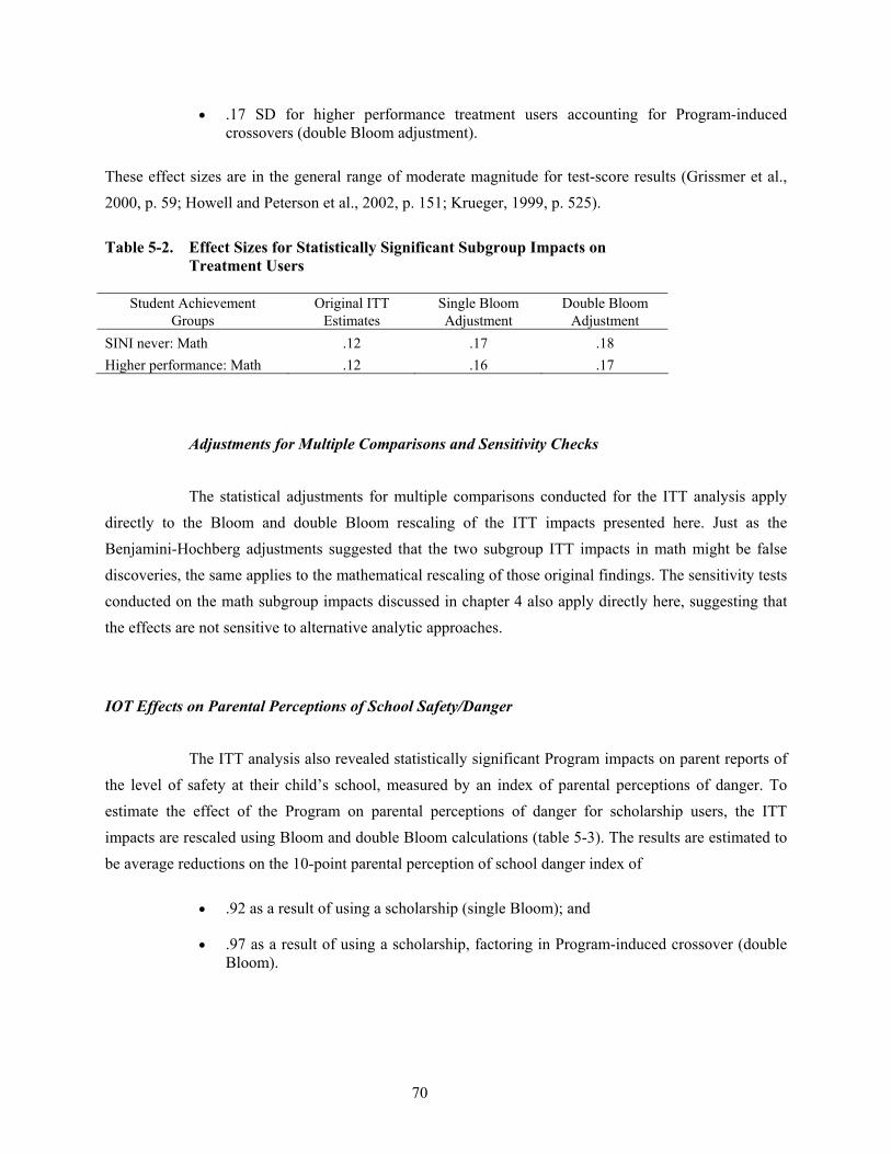
70
• .17 SD for higher performance treatment users accounting for Program-induced crossovers (double Bloom adjustment).
These effect sizes are in the general range of moderate magnitude for test-score results (Grissmer et al., 2000, p. 59; Howell and Peterson et al., 2002, p. 151; Krueger, 1999, p. 525). Table 5-2. Effect Sizes for Statistically Significant Subgroup Impacts on
Treatment Users
Student Achievement Groups
Original ITT Estimates
Single Bloom Adjustment
Double Bloom Adjustment
SINI never: Math .12 .17 .18 Higher performance: Math .12 .16 .17
Adjustments for Multiple Comparisons and Sensitivity Checks The statistical adjustments for multiple comparisons conducted for the ITT analysis apply
directly to the Bloom and double Bloom rescaling of the ITT impacts presented here. Just as the Benjamini-Hochberg adjustments suggested that the two subgroup ITT impacts in math might be false discoveries, the same applies to the mathematical rescaling of those original findings. The sensitivity tests conducted on the math subgroup impacts discussed in chapter 4 also apply directly here, suggesting that the effects are not sensitive to alternative analytic approaches.
IOT Effects on Parental Perceptions of School Safety/Danger
The ITT analysis also revealed statistically significant Program impacts on parent reports of the level of safety at their child’s school, measured by an index of parental perceptions of danger. To estimate the effect of the Program on parental perceptions of danger for scholarship users, the ITT impacts are rescaled using Bloom and double Bloom calculations (table 5-3). The results are estimated to be average reductions on the 10-point parental perception of school danger index of
• .92 as a result of using a scholarship (single Bloom); and
• .97 as a result of using a scholarship, factoring in Program-induced crossover (double Bloom).
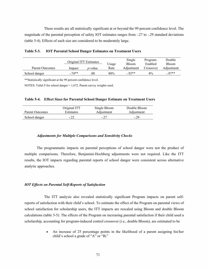
71
These results are all statistically significant at or beyond the 99 percent confidence level. The magnitude of the parental perception of safety IOT estimates ranges from -.27 to -.29 standard deviations (table 5-4). Effects of such size are considered to be moderately large.
Table 5-3. IOT Parental School Danger Estimates on Treatment Users
Original ITT Estimates
Parent Outcomes Impact p-value Usage Rate
Single Bloom
Adjustment
Program-Enabled
Crossover
Double Bloom
Adjustment School danger -.74** .00 80% -.92** 4% -.97**
**Statistically significant at the 99 percent confidence level.
NOTES: Valid N for school danger = 1,672. Parent survey weights used.
Table 5-4. Effect Sizes for Parental School Danger Estimate on Treatment Users
Parent Outcomes Original ITT
Estimates Single Bloom Adjustment
Double Bloom Adjustment
School danger -.22 -.27 -.29
Adjustments for Multiple Comparisons and Sensitivity Checks
The programmatic impacts on parental perceptions of school danger were not the product of multiple comparisons. Therefore, Benjamini-Hochberg adjustments were not required. Like the ITT results, the IOT impacts regarding parental reports of school danger were consistent across alternative analytic approaches.
IOT Effects on Parental Self-Reports of Satisfaction
The ITT analysis also revealed statistically significant Program impacts on parent self-reports of satisfaction with their child’s school. To estimate the effect of the Program on parental views of school satisfaction for scholarship users, the ITT impacts are rescaled using Bloom and double Bloom calculations (table 5-5). The effects of the Program on increasing parental satisfaction if their child used a scholarship, accounting for program-induced control crossover (i.e., double Bloom), are estimated to be
• An increase of 25 percentage points in the likelihood of a parent assigning his/her
child’s school a grade of “A” or “B;”
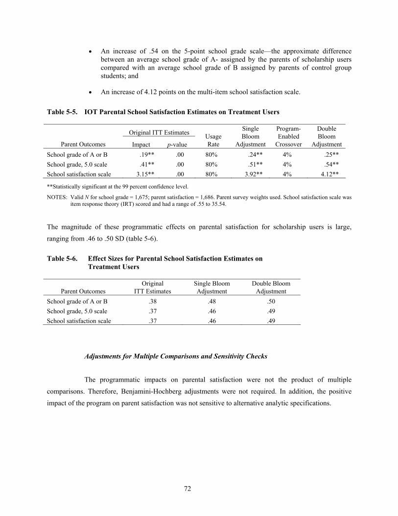
72
• An increase of .54 on the 5-point school grade scale—the approximate difference between an average school grade of A- assigned by the parents of scholarship users compared with an average school grade of B assigned by parents of control group students; and
• An increase of 4.12 points on the multi-item school satisfaction scale.
Table 5-5. IOT Parental School Satisfaction Estimates on Treatment Users
Original ITT Estimates
Parent Outcomes Impact p-value Usage Rate
Single Bloom
Adjustment
Program-Enabled
Crossover
Double Bloom
Adjustment School grade of A or B .19** .00 80% .24** 4% .25** School grade, 5.0 scale .41** .00 80% .51** 4% .54** School satisfaction scale 3.15** .00 80% 3.92** 4% 4.12**
**Statistically significant at the 99 percent confidence level.
NOTES: Valid N for school grade = 1,675; parent satisfaction = 1,686. Parent survey weights used. School satisfaction scale was item response theory (IRT) scored and had a range of .55 to 35.54.
The magnitude of these programmatic effects on parental satisfaction for scholarship users is large, ranging from .46 to .50 SD (table 5-6). Table 5-6. Effect Sizes for Parental School Satisfaction Estimates on
Treatment Users
Parent Outcomes Original
ITT Estimates Single Bloom Adjustment
Double Bloom Adjustment
School grade of A or B .38 .48 .50 School grade, 5.0 scale .37 .46 .49 School satisfaction scale .37 .46 .49
Adjustments for Multiple Comparisons and Sensitivity Checks
The programmatic impacts on parental satisfaction were not the product of multiple comparisons. Therefore, Benjamini-Hochberg adjustments were not required. In addition, the positive impact of the program on parent satisfaction was not sensitive to alternative analytic specifications.
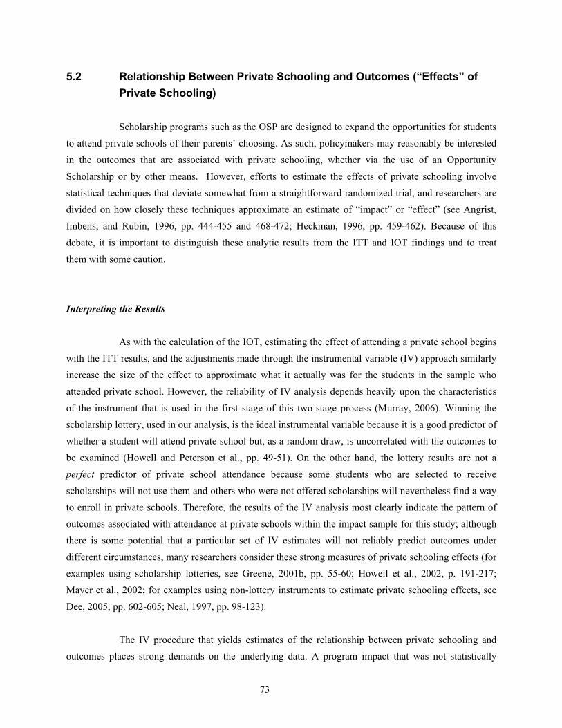
73
5.2 Relationship Between Private Schooling and Outcomes (“Effects” of Private Schooling)
Scholarship programs such as the OSP are designed to expand the opportunities for students to attend private schools of their parents’ choosing. As such, policymakers may reasonably be interested in the outcomes that are associated with private schooling, whether via the use of an Opportunity Scholarship or by other means. However, efforts to estimate the effects of private schooling involve statistical techniques that deviate somewhat from a straightforward randomized trial, and researchers are divided on how closely these techniques approximate an estimate of “impact” or “effect” (see Angrist, Imbens, and Rubin, 1996, pp. 444-455 and 468-472; Heckman, 1996, pp. 459-462). Because of this debate, it is important to distinguish these analytic results from the ITT and IOT findings and to treat them with some caution.
Interpreting the Results
As with the calculation of the IOT, estimating the effect of attending a private school begins with the ITT results, and the adjustments made through the instrumental variable (IV) approach similarly increase the size of the effect to approximate what it actually was for the students in the sample who attended private school. However, the reliability of IV analysis depends heavily upon the characteristics of the instrument that is used in the first stage of this two-stage process (Murray, 2006). Winning the scholarship lottery, used in our analysis, is the ideal instrumental variable because it is a good predictor of whether a student will attend private school but, as a random draw, is uncorrelated with the outcomes to be examined (Howell and Peterson et al., pp. 49-51). On the other hand, the lottery results are not a perfect predictor of private school attendance because some students who are selected to receive scholarships will not use them and others who were not offered scholarships will nevertheless find a way to enroll in private schools. Therefore, the results of the IV analysis most clearly indicate the pattern of outcomes associated with attendance at private schools within the impact sample for this study; although there is some potential that a particular set of IV estimates will not reliably predict outcomes under different circumstances, many researchers consider these strong measures of private schooling effects (for examples using scholarship lotteries, see Greene, 2001b, pp. 55-60; Howell et al., 2002, p. 191-217; Mayer et al., 2002; for examples using non-lottery instruments to estimate private schooling effects, see Dee, 2005, pp. 602-605; Neal, 1997, pp. 98-123).
The IV procedure that yields estimates of the relationship between private schooling and
outcomes places strong demands on the underlying data. A program impact that was not statistically
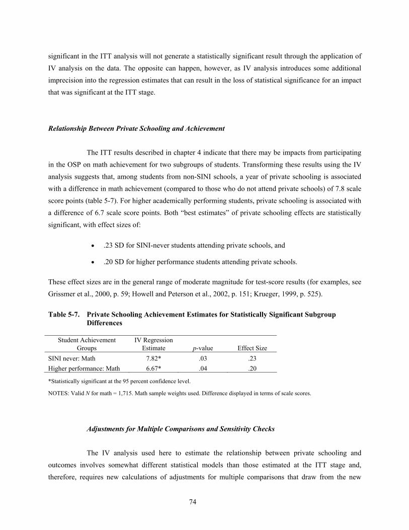
74
significant in the ITT analysis will not generate a statistically significant result through the application of IV analysis on the data. The opposite can happen, however, as IV analysis introduces some additional imprecision into the regression estimates that can result in the loss of statistical significance for an impact that was significant at the ITT stage.
Relationship Between Private Schooling and Achievement
The ITT results described in chapter 4 indicate that there may be impacts from participating in the OSP on math achievement for two subgroups of students. Transforming these results using the IV analysis suggests that, among students from non-SINI schools, a year of private schooling is associated with a difference in math achievement (compared to those who do not attend private schools) of 7.8 scale score points (table 5-7). For higher academically performing students, private schooling is associated with a difference of 6.7 scale score points. Both “best estimates” of private schooling effects are statistically significant, with effect sizes of:
• .23 SD for SINI-never students attending private schools, and
• .20 SD for higher performance students attending private schools.
These effect sizes are in the general range of moderate magnitude for test-score results (for examples, see Grissmer et al., 2000, p. 59; Howell and Peterson et al., 2002, p. 151; Krueger, 1999, p. 525).
Table 5-7. Private Schooling Achievement Estimates for Statistically Significant Subgroup
Differences
Student Achievement Groups
IV Regression Estimate p-value Effect Size
SINI never: Math 7.82* .03 .23 Higher performance: Math 6.67* .04 .20
*Statistically significant at the 95 percent confidence level.
NOTES: Valid N for math = 1,715. Math sample weights used. Difference displayed in terms of scale scores.
Adjustments for Multiple Comparisons and Sensitivity Checks
The IV analysis used here to estimate the relationship between private schooling and outcomes involves somewhat different statistical models than those estimated at the ITT stage and, therefore, requires new calculations of adjustments for multiple comparisons that draw from the new
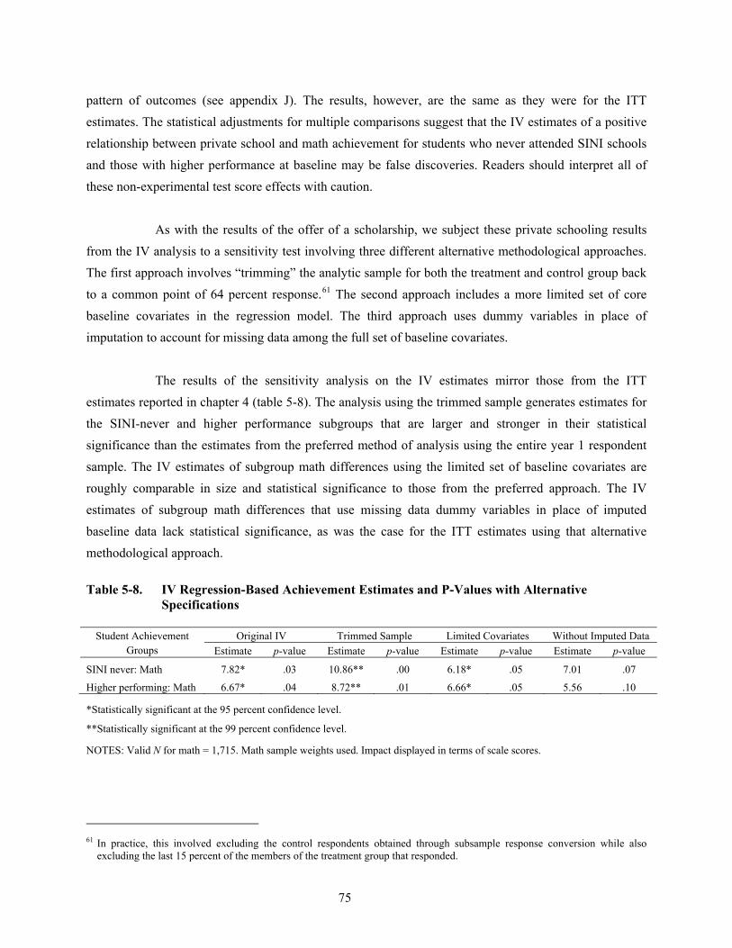
75
pattern of outcomes (see appendix J). The results, however, are the same as they were for the ITT estimates. The statistical adjustments for multiple comparisons suggest that the IV estimates of a positive relationship between private school and math achievement for students who never attended SINI schools and those with higher performance at baseline may be false discoveries. Readers should interpret all of these non-experimental test score effects with caution.
As with the results of the offer of a scholarship, we subject these private schooling results
from the IV analysis to a sensitivity test involving three different alternative methodological approaches. The first approach involves “trimming” the analytic sample for both the treatment and control group back to a common point of 64 percent response.61 The second approach includes a more limited set of core baseline covariates in the regression model. The third approach uses dummy variables in place of imputation to account for missing data among the full set of baseline covariates.
The results of the sensitivity analysis on the IV estimates mirror those from the ITT
estimates reported in chapter 4 (table 5-8). The analysis using the trimmed sample generates estimates for the SINI-never and higher performance subgroups that are larger and stronger in their statistical significance than the estimates from the preferred method of analysis using the entire year 1 respondent sample. The IV estimates of subgroup math differences using the limited set of baseline covariates are roughly comparable in size and statistical significance to those from the preferred approach. The IV estimates of subgroup math differences that use missing data dummy variables in place of imputed baseline data lack statistical significance, as was the case for the ITT estimates using that alternative methodological approach.
Table 5-8. IV Regression-Based Achievement Estimates and P-Values with Alternative
Specifications
Original IV Trimmed Sample Limited Covariates Without Imputed Data Student Achievement Groups Estimate p-value Estimate p-value Estimate p-value Estimate p-value
SINI never: Math 7.82* .03 10.86** .00 6.18* .05 7.01 .07
Higher performing: Math 6.67* .04 8.72** .01 6.66* .05 5.56 .10
*Statistically significant at the 95 percent confidence level.
**Statistically significant at the 99 percent confidence level.
NOTES: Valid N for math = 1,715. Math sample weights used. Impact displayed in terms of scale scores.
61 In practice, this involved excluding the control respondents obtained through subsample response conversion while also
excluding the last 15 percent of the members of the treatment group that responded.
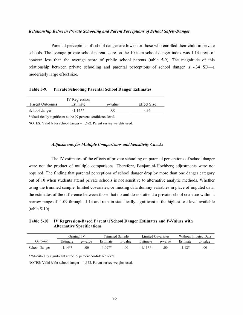
76
Relationship Between Private Schooling and Parent Perceptions of School Safety/Danger
Parental perceptions of school danger are lower for those who enrolled their child in private schools. The average private school parent score on the 10-item school danger index was 1.14 areas of concern less than the average score of public school parents (table 5-9). The magnitude of this relationship between private schooling and parental perceptions of school danger is -.34 SD—a moderately large effect size.
Table 5-9. Private Schooling Parental School Danger Estimates
Parent Outcomes IV Regression
Estimate p-value Effect Size School danger -1.14** .00 -.34 **Statistically significant at the 99 percent confidence level.
NOTES: Valid N for school danger = 1,672. Parent survey weights used.
Adjustments for Multiple Comparisons and Sensitivity Checks
The IV estimates of the effects of private schooling on parental perceptions of school danger were not the product of multiple comparisons. Therefore, Benjamini-Hochberg adjustments were not required. The finding that parental perceptions of school danger drop by more than one danger category out of 10 when students attend private schools is not sensitive to alternative analytic methods. Whether using the trimmed sample, limited covariates, or missing data dummy variables in place of imputed data, the estimates of the difference between those that do and do not attend a private school coalesce within a narrow range of -1.09 through -1.14 and remain statistically significant at the highest test level available (table 5-10).
Table 5-10. IV Regression-Based Parental School Danger Estimates and P-Values with
Alternative Specifications
Original IV Trimmed Sample Limited Covariates Without Imputed Data Outcome Estimate p-value Estimate p-value Estimate p-value Estimate p-value
School Danger -1.14** .00 -1.09** .00 -1.11** .00 -1.12* .00
**Statistically significant at the 99 percent confidence level.
NOTES: Valid N for school danger = 1,672. Parent survey weights used.
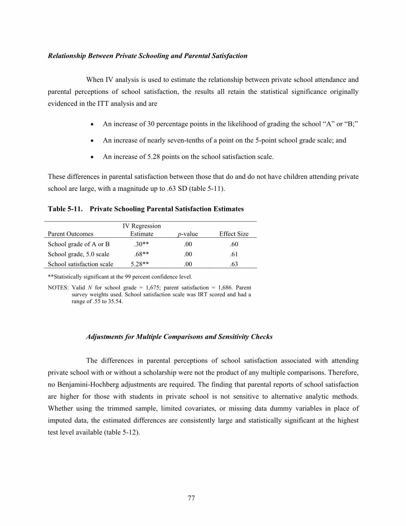
77
Relationship Between Private Schooling and Parental Satisfaction
When IV analysis is used to estimate the relationship between private school attendance and parental perceptions of school satisfaction, the results all retain the statistical significance originally evidenced in the ITT analysis and are
• An increase of 30 percentage points in the likelihood of grading the school “A” or “B;”
• An increase of nearly seven-tenths of a point on the 5-point school grade scale; and
• An increase of 5.28 points on the school satisfaction scale.
These differences in parental satisfaction between those that do and do not have children attending private school are large, with a magnitude up to .63 SD (table 5-11). Table 5-11. Private Schooling Parental Satisfaction Estimates
Parent Outcomes IV Regression
Estimate p-value
Effect Size School grade of A or B .30** .00 .60 School grade, 5.0 scale .68** .00 .61 School satisfaction scale 5.28** .00 .63
**Statistically significant at the 99 percent confidence level.
NOTES: Valid N for school grade = 1,675; parent satisfaction = 1,686. Parent survey weights used. School satisfaction scale was IRT scored and had a range of .55 to 35.54.
Adjustments for Multiple Comparisons and Sensitivity Checks
The differences in parental perceptions of school satisfaction associated with attending private school with or without a scholarship were not the product of any multiple comparisons. Therefore, no Benjamini-Hochberg adjustments are required. The finding that parental reports of school satisfaction are higher for those with students in private school is not sensitive to alternative analytic methods. Whether using the trimmed sample, limited covariates, or missing data dummy variables in place of imputed data, the estimated differences are consistently large and statistically significant at the highest test level available (table 5-12).
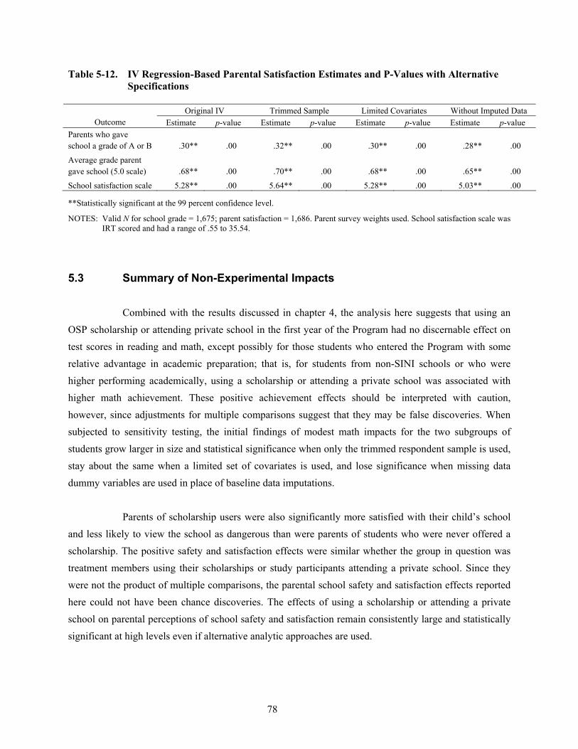
78
Table 5-12. IV Regression-Based Parental Satisfaction Estimates and P-Values with Alternative Specifications
Original IV Trimmed Sample Limited Covariates Without Imputed Data
Outcome Estimate p-value Estimate p-value Estimate p-value Estimate p-value Parents who gave school a grade of A or B .30** .00 .32** .00 .30** .00 .28** .00
Average grade parent gave school (5.0 scale) .68** .00 .70** .00 .68** .00 .65** .00
School satisfaction scale 5.28** .00 5.64** .00 5.28** .00 5.03** .00
**Statistically significant at the 99 percent confidence level.
NOTES: Valid N for school grade = 1,675; parent satisfaction = 1,686. Parent survey weights used. School satisfaction scale was IRT scored and had a range of .55 to 35.54.
5.3 Summary of Non-Experimental Impacts
Combined with the results discussed in chapter 4, the analysis here suggests that using an OSP scholarship or attending private school in the first year of the Program had no discernable effect on test scores in reading and math, except possibly for those students who entered the Program with some relative advantage in academic preparation; that is, for students from non-SINI schools or who were higher performing academically, using a scholarship or attending a private school was associated with higher math achievement. These positive achievement effects should be interpreted with caution, however, since adjustments for multiple comparisons suggest that they may be false discoveries. When subjected to sensitivity testing, the initial findings of modest math impacts for the two subgroups of students grow larger in size and statistical significance when only the trimmed respondent sample is used, stay about the same when a limited set of covariates is used, and lose significance when missing data dummy variables are used in place of baseline data imputations.
Parents of scholarship users were also significantly more satisfied with their child’s school
and less likely to view the school as dangerous than were parents of students who were never offered a scholarship. The positive safety and satisfaction effects were similar whether the group in question was treatment members using their scholarships or study participants attending a private school. Since they were not the product of multiple comparisons, the parental school safety and satisfaction effects reported here could not have been chance discoveries. The effects of using a scholarship or attending a private school on parental perceptions of school safety and satisfaction remain consistently large and statistically significant at high levels even if alternative analytic approaches are used.
79
As described in chapter 4, the absence of achievement impacts for overall OSP scholarship use fit into a series of inconsistent results on achievement impacts demonstrated by other scholarship experiments after 1 year, while the positive parent satisfaction and safety effects are all consistent with those earlier studies.

80
81
References
Angrist, Joshua, Guido Imbens, and Donald B. Rubin. “Identification of Causal Effects Using
Instrumental Variables.” Journal of the American Statistical Association 1996, 91: 444-455. Barnard, John, Constantine E. Frangakis, Jennifer L. Hill, and Donald B. Rubin. “Principal Stratification
Approach to Broken Randomized Experiments: A Case Study of School Choice Vouchers in New York City.” Journal of the American Statistical Association 2003, 98: 462.
Benjamini, Yoav, and Yosef Hochberg. “Controlling for the False Discovery Rate: A Practical and
Powerful Approach to Multiple Testing.” Journal of the Royal Statistical Society, Series B (Methodological) 1995, 57(1): 289-300.
Bloom, Howard S. "Accounting for No-Shows in Experimental Evaluation Designs." Evaluation Review
1984, 8(2): 225-246. Greene, Jay P. “The Effect of School Choice: An Evaluation of the Charlotte Children’s Scholarship
Fund.” Civic Report No. 12. New York, NY: Manhattan Institute for Policy Research, 2000. Greene, Jay P. “The Hidden Research Consensus for School Choice.” In Paul E. Peterson and David E.
Campbell, eds., Charters, Vouchers, and Public Education. Washington, DC: Brookings, 2001. Grissmer, David W., Ann Flanagan, Jennifer Kawata, and Stephanie Williamson. Improving Student
Achievement: What NAEP Test Scores Tell Us. Santa Monica, CA: RAND Corporation, 2000. Hambleton, Ronald K., Hariharan Swaminathan, and Jane H. Rogers. Fundamentals of Item Response
Theory. Newbury Park, CA: Sage Publications, 1991. Howell, William G., Patrick J. Wolf, David E. Campbell, and Paul E. Peterson. “School Vouchers and
Academic Performance: Results from Three Randomized Field Trials.” Journal of Policy Analysis and Management 2002, 21(2): 191-217.
Howell, William G., and Paul E. Peterson, with Patrick J. Wolf and David E. Campbell. The Education
Gap: Vouchers and Urban Schools. Washington, DC: Brookings, 2002. Howell, William G., and Paul E. Peterson. “Uses of Theory in Randomized Field Trials: Lessons from
School Voucher Research on Disaggregation, Missing Data, and the Generalization of Findings.” American Behavioral Scientist 2004, 47(5): 634-657.
Johnson, Michael D., and Claes Fornell. “A Framework for Comparing Customer Satisfaction across
Individuals and Product Categories.” Journal of Economic Psychology 1991, 12(2): 267-286. Kling, Jeffrey R., Jens Ludwig, and Lawrence F. Katz, “Neighborhood Effects on Crime for Female and
Male Youth: Evidence from a Randomized Housing Voucher Experiment.” Quarterly Journal of Economics 2005, 120(1): 87-130.
82
Krueger, Alan B. “Experimental Estimates of Education Production Functions.” Quarterly Journal of Economics 1999, 114 (2): 497-532.
Krueger, Alan B., and Pei Zhu. “Another Look at the New York City School Voucher Experiment.”
American Behavioral Scientist 2004, 47(5): 658-698. Krueger, Alan B., and Pei Zhu. “Inefficiency, Subsample Selection Bias, and Nonrobustness: A Response
to Paul E. Peterson and William G. Howell.” American Behavioral Scientist 2004, 47(5): 718-728.
Liang, Kung-Yee, and Scott L. Zeger, “Longitudinal Data Analysis Using Generalized Linear Models.”
Biometrika 1986, 73(1): 13-22. Mayer, Daniel P., Paul E. Peterson, David E. Myers, Christina Clark Tuttle, and William G. Howell.
School Choice in New York City After Three Years: An Evaluation of the School Choice Scholarships Program. MPR Reference No. 8404-045. Cambridge, MA: Mathematica Policy Research, 2002.
Murray, Michael P. “Avoiding Invalid Instruments and Coping with Weak Instruments.” Journal of
Economic Perspectives 20(4): 111-132. Peterson, Paul E., David Myers, William G. Howell, and Daniel P. Mayer. “The Effects of School Choice
in New York City.” In Susan E. Mayer and Paul E. Peterson, eds., Earning and Learning: How Schools Matter. Washington, DC: Brookings, 1999.
Peterson, Paul E., and William G. Howell. “Efficiency, Bias, and Classification Schemes: A Response to
Alan B. Krueger and Pei Zhu. American Behavioral Scientist 2004, 47(5): 699-717. Rouse, Cecelia E. “Private School Vouchers and Student Achievement: An Evaluation of the Milwaukee
Parental Choice Program.” Quarterly Journal of Economics 1998, 113(2): 553-602. Sanbonmatsu, Lisa, Jeffrey R. Kling, Greg J. Duncan, and Jeanne Brooks-Gunn. “Neighborhoods and
Academic Achievement: Results from the Moving to Opportunity Experiment.” Journal of Human Resources 2006, 41(4): 649-691.
Spector, Paul E. Summated Rating Scale Construction: An Introduction. Newbury Park, CA: Sage
Publications, 1992. Stewart, Thomas, Patrick J. Wolf, and Stephen Q. Cornman. Parent and Student Voices on the First Year
of the DC Opportunity Scholarship Program. SCDP Report 05-01. Washington, DC: School Choice Demonstration Project, Georgetown University, 2005. Available online at [http://www.georgetown.edu/research/scdp/PSV-FirstYear.html].
Thurstone, L.L. "A Method of Scaling Psychological and Educational Tests." Journal of Educational
Psychology 1925, 16: 433-451. U.S. Department of Health and Human Services, Administration for Children and Families, Office of
Planning, Research and Evaluation. Head Start Impact Study: First Year Findings. Washington, DC: 2005. Available online at [http://www.acf.hhs.gov/programs/opre/hs/impact_study/reports/ first_yr_finds/first_yr_finds.pdf].
83
White, Halbert. “Maximum Likelihood Estimation of Misspecified Models. Econometrica 1982, 50(1): 1-25.
Witte, John F. The Market Approach to Education: An Analysis of America’s First Voucher Program.
Princeton, NJ: Princeton University Press, 2001. Wolf, Patrick, Babette Gutmann, Nada Eissa, Michael Puma, and Marsha Silverberg. Evaluation of the
DC Opportunity Scholarship Program: First Year Report on Participation. U.S. Department of Education, National Center for Education Evaluation and Regional Assistance. Washington, DC: U.S. Government Printing Office, 2005. Available online at: [http://ies.ed.gov/ncee/ pubs/dc_choice.asp].
Wolf, Patrick, Babette Gutmann, Michael Puma, and Marsha Silverberg. Evaluation of the DC
Opportunity Scholarship Program: Second Year Report on Participation. U.S. Department of Education, National Center for Education Evaluation and Regional Assistance, NCEE 2006-4003. Washington, DC: U.S. Government Printing Office, 2006. Available online at: [http://ies.ed.gov/ncee/pdf/20064003.pdf].
Wolf, Patrick J., Paul E. Peterson, and Martin R. West. Results of a School Voucher Experiment: The
Case of Washington, D.C. After Two Years. Paper delivered at the National Center for Education Statistics 2001 Data Conference, Mayflower Hotel, Washington, DC: July 25-27, 2001. Available online at: [http://papers.ssrn.com/sol3/papers.cfm?abstract_id=313822].
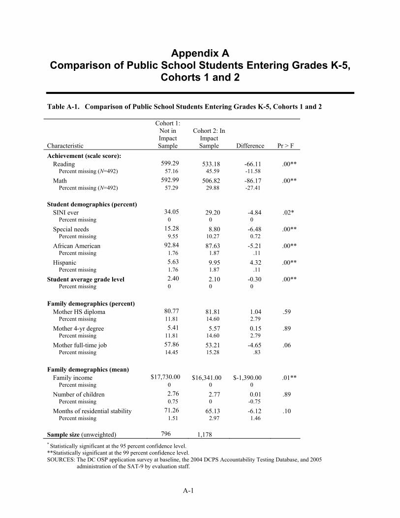
A-1
Appendix A Comparison of Public School Students Entering Grades K-5,
Cohorts 1 and 2
Table A-1. Comparison of Public School Students Entering Grades K-5, Cohorts 1 and 2
Characteristic
Cohort 1: Not in Impact Sample
Cohort 2: In Impact Sample Difference Pr > F
Achievement (scale score): Reading 599.29 533.18 -66.11 .00**
Percent missing (N=492) 57.16 45.59 -11.58
Math 592.99 506.82 -86.17 .00** Percent missing (N=492) 57.29 29.88 -27.41
Student demographics (percent)
SINI ever 34.05 29.20 -4.84 .02* Percent missing 0 0 0
Special needs 15.28 8.80 -6.48 .00** Percent missing 9.55 10.27 0.72
African American 92.84 87.63 -5.21 .00** Percent missing 1.76 1.87 .11
Hispanic 5.63 9.95 4.32 .00** Percent missing 1.76 1.87 .11
Student average grade level 2.40 2.10 -0.30 .00** Percent missing 0 0 0
Family demographics (percent)
Mother HS diploma 80.77 81.81 1.04 .59 Percent missing 11.81 14.60 2.79
Mother 4-yr degree 5.41 5.57 0.15 .89 Percent missing 11.81 14.60 2.79
Mother full-time job 57.86 53.21 -4.65 .06 Percent missing 14.45 15.28 .83
Family demographics (mean) Family income $17,730.00 $16,341.00 $-1,390.00 .01**
Percent missing 0 0 0
Number of children 2.76 2.77 0.01 .89 Percent missing 0.75 0 -0.75
Months of residential stability 71.26 65.13 -6.12 .10 Percent missing 1.51 2.97 1.46
Sample size (unweighted) 796 1,178 * Statistically significant at the 95 percent confidence level. **Statistically significant at the 99 percent confidence level. SOURCES: The DC OSP application survey at baseline, the 2004 DCPS Accountability Testing Database, and 2005
administration of the SAT-9 by evaluation staff.

B-1
Appendix B Study Power
The goals of statistical power analysis and sample size estimation are to determine how large a sample is needed to make accurate and reliable statistical judgments and how likely it is that a statistical test will detect effects of a given magnitude. Formally, power is the probability of rejecting the null hypothesis (the initial assumption that the treatment has no effect) if the treatment actually has an effect. Power is estimated at the early stages of a study, based on assumptions regarding the amount of data and the strength of relationships within those data. Power estimates establish reasonable expectations, prior to actual data collection, regarding how large true programmatic effects would need to be in order for the data and analysis to reveal them.
Minimum detectable effects (MDEs) are a simple way to express the statistical precision or
“power” of an impact study design. Intuitively, an MDE is the smallest program impact or “effect size” that could be measured with confidence given random sampling and statistical estimation error. Study power itself is much like the power of a microscope—the greater the power, the smaller the objects that can be detected. Thus, MDEs of a small fraction of a standard deviation (SD), such as .10 SD, signal greater study power than do larger MDEs, such as .30 SD.
Although the evaluation will analyze outcomes such as test scores in every year post-
baseline, for simplicity, we present the power analysis numbers for two representative years―the first and third outcome years. Central to analytic power is the sample size of study participants who actually provide outcome information in a given year. Thus, this power analysis factors in expected study attrition and non-response over time. The analysis also takes account of the correlation between baseline test scores and outcome test scores. By including baseline test scores in the statistical estimation of outcome test scores, analysts make the estimation of the impact of the treatment on the outcome more precise, thus increasing power (see Howell et al., 2002, pp. 191-217).1
1 The calculation of study power accounted for anticipated levels of non-response, likely sample attrition, and the use of
covariates in the analytical model, drawing upon data from an earlier experimental evaluation of a privately funded school voucher program in the District of Columbia. The statistical models run on those previous voucher data were less precise than the models run in the actual analyses of these data from this new voucher evaluation. As a result, the MDEs generated prior to the actual analysis and presented here are conservative estimates of the likely MDEs for the evaluation, which will be somewhat lower. A relatively low MDE indicates a more evidence-rich and better-powered analysis.

B-2
Because baseline test scores were obtained for most, but not all, members of the impact sample, the power analysis is conducted under conditions of the absence of baseline test scores as well as the presence of baseline test scores. Leaving out the baseline test scores does not measurably change the MDEs, so we present the MDEs with baseline test scores. (We have imputed missing baseline data, thereby producing an analysis sample with complete baseline data.)
A majority of the students in the impact sample (56 percent) have siblings who also are
participating in the evaluation. The test scores of children from the same family tend to be correlated with each other, since siblings share some of the same genes and experience similar home environments that affect learning. Thus, the power analysis that we conducted adjusts for the fact that test-score clustering within families reduces the amount of independent information that siblings contribute to the evaluation.
If all else is equal, power is greatest when the treatment and control groups are the same size.
This condition is not met in this evaluation. The evaluation of the DC Opportunity Scholarship Program (OSP) differs from other evaluations that recruit participants until they achieve required samples. Instead, it is based on the actual number of applicants, private school slots available, and the ratio of those two in the 2 first years of the Program. Since the treatment group is 50 percent larger than the control group, our analysis will have slightly less power than a study with a comparable number of participants equally distributed across the treatment condition.
Finally, these power estimates do not account for the reality that some students in the
treatment group who are offered the scholarship decline to use it (referred to as “no shows” in the experimental literature). Assuming that the Program has no impact on the students who decline to use a scholarship, each study participant who is a treatment decliner generates outcome data that have the practical effect of reducing the intention-to-treat (ITT) impact estimate toward zero. Thus, experimental evaluations of programs that experience high levels of “no shows” often fail to report statistically significant programmatic impacts simply because fewer than expected members of the treatment group actually use the programmatic treatment (Howell and Peterson et al., 2002, pp. 44, 146-147).2 Low treatment usage rates do not reduce the analytic power of ITT estimates. They make findings of Program impact less likely because they reduce the size of the average impact of the Program across the entire treatment group of users and non-users. Thus, a high-powered analysis is likely to detect programmatic impacts even under conditions of moderate levels of Program attrition because such an analysis will be able to detect relatively small average treatment effects. 2 For example, in the previous experimental evaluation of the partial-tuition scholarship program in Washington, DC, only 29
percent of the students assigned to the treatment group were using their scholarships by the third year of the evaluation. Not surprisingly, no test-score impacts were identified in Year 3 of that evaluation.
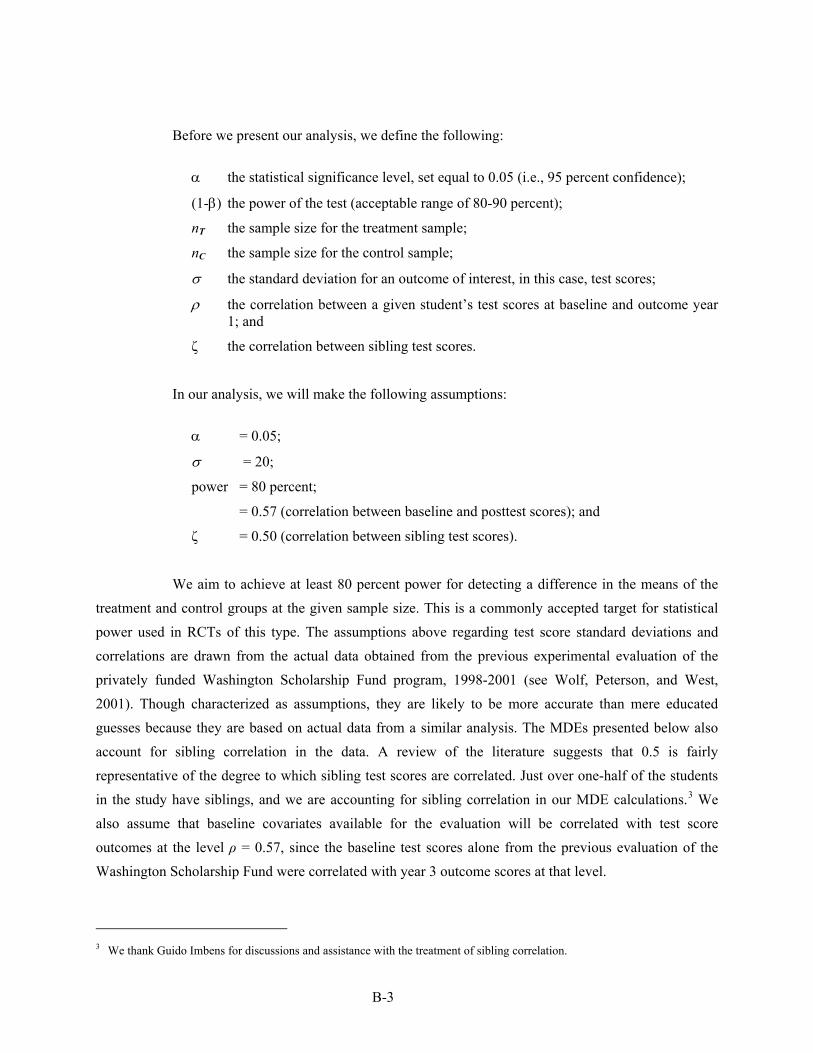
B-3
Before we present our analysis, we define the following:
α the statistical significance level, set equal to 0.05 (i.e., 95 percent confidence);
(1-β) the power of the test (acceptable range of 80-90 percent);
nT the sample size for the treatment sample;
nC the sample size for the control sample;
σ the standard deviation for an outcome of interest, in this case, test scores;
ρ the correlation between a given student’s test scores at baseline and outcome year 1; and
ζ the correlation between sibling test scores.
In our analysis, we will make the following assumptions:
α = 0.05;
σ = 20;
power = 80 percent;
= 0.57 (correlation between baseline and posttest scores); and
ζ = 0.50 (correlation between sibling test scores).
We aim to achieve at least 80 percent power for detecting a difference in the means of the
treatment and control groups at the given sample size. This is a commonly accepted target for statistical power used in RCTs of this type. The assumptions above regarding test score standard deviations and correlations are drawn from the actual data obtained from the previous experimental evaluation of the privately funded Washington Scholarship Fund program, 1998-2001 (see Wolf, Peterson, and West, 2001). Though characterized as assumptions, they are likely to be more accurate than mere educated guesses because they are based on actual data from a similar analysis. The MDEs presented below also account for sibling correlation in the data. A review of the literature suggests that 0.5 is fairly representative of the degree to which sibling test scores are correlated. Just over one-half of the students in the study have siblings, and we are accounting for sibling correlation in our MDE calculations.3 We also assume that baseline covariates available for the evaluation will be correlated with test score outcomes at the level ρ = 0.57, since the baseline test scores alone from the previous evaluation of the Washington Scholarship Fund were correlated with year 3 outcome scores at that level.
3 We thank Guido Imbens for discussions and assistance with the treatment of sibling correlation.
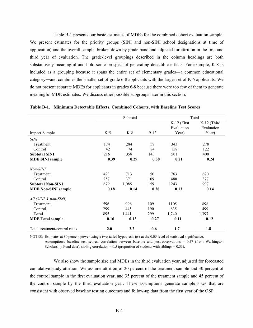
B-4
Table B-1 presents our basic estimates of MDEs for the combined cohort evaluation sample. We present estimates for the priority groups (SINI and non-SINI school designations at time of application) and the overall sample, broken down by grade band and adjusted for attrition in the first and third year of evaluation. The grade-level groupings described in the column headings are both substantively meaningful and hold some prospect of generating detectible effects. For example, K-8 is included as a grouping because it spans the entire set of elementary grades―a common educational category―and combines the smaller set of grade 6-8 applicants with the larger set of K-5 applicants. We do not present separate MDEs for applicants in grades 6-8 because there were too few of them to generate meaningful MDE estimates. We discuss other possible subgroups later in this section.
Table B-1. Minimum Detectable Effects, Combined Cohorts, with Baseline Test Scores Subtotal Total
Impact Sample K-5 K-8 9-12
K-12 (First Evaluation
Year)
K-12 (Third Evaluation
Year) SINI
Treatment 174 284 59 343 278 Control 42 74 84 158 122
Subtotal SINI 216 358 143 501 400 MDE SINI sample 0.39 0.29 0.38 0.21 0.24 Non-SINI
Treatment 423 713 50 763 620 Control 257 371 109 480 377
Subtotal Non-SINI 679 1,085 159 1243 997 MDE Non-SINI sample 0.18 0.14 0.38 0.13 0.14 All (SINI & non-SINI)
Treatment 596 996 109 1105 898 Control 299 445 190 635 499 Total 895 1,441 299 1,740 1,397
MDE Total sample 0.16 0.13 0.27 0.11 0.12 Total treatment/control ratio 2.0 2.2 0.6 1.7 1.8
NOTES: Estimates at 80 percent power using a two-tailed hypothesis test at the 0.05 level of statistical significance. Assumptions: baseline test scores, correlation between baseline and post-observations = 0.57 (from Washington
Scholarship Fund data); sibling correlation = 0.5 (proportion of students with siblings = 0.33).
We also show the sample size and MDEs in the third evaluation year, adjusted for forecasted
cumulative study attrition. We assume attrition of 20 percent of the treatment sample and 30 percent of the control sample in the first evaluation year, and 35 percent of the treatment sample and 45 percent of the control sample by the third evaluation year. These assumptions generate sample sizes that are consistent with observed baseline testing outcomes and follow-up data from the first year of the OSP.

B-5
The subsample of participants who were attending schools already designated SINI at the time of application is insufficient to provide power to identify anything smaller than a moderately large effect (.21 to .24 SD). Coupled with the fact that official SINI designations lag actual school performance by a year, this finding led the research team to develop and use the SINI-ever variable in the analysis of possible subgroup effects by SINI status. The combined non-SINI subsample generates viable MDEs for K-12 in year 1 (0.13 of a standard deviation), K-12 in year 3 (0.14 of a standard deviation), and K-8 in year 1 (0.14 of a standard deviation). The complete combined sample is forecasted to produce relatively modest MDEs for K-12 in year 1 (0.1 of a standard deviation) and in year 3 (0.12 of a standard deviation) as well as moderate MDEs for the K-5, K-8, and 6-12 subsamples of the combined cohort data.
To place these estimated effect sizes in context, an effect of 0.13 to 0.15 of a standard
deviation equates to a Normal Curve Equivalent (NCE) difference of 2.73 to 3.15 NCE points.4 Converting NCEs to a change in percentile ranks depends on where on the overall distribution the observed change occurs. For example, if the control group was, on average, at the 20th percentile, a gain of 3.15 NCEs would bring it up to about the 24th percentile. Such a gain is likely to be considered modest but educationally meaningful.
Our analysis also shows that the Cohort 1 impact sample, by itself, cannot be used to
estimate program effects within reasonable bounds. A number of prominent evaluations of educational interventions have reported statistically significant impacts near or within the range of 0.15 to 0.20 standard deviations over 1 to 3 years. Such impacts are generally characterized as moderate in size and policy relevant (for examples, see Grissmer et al., 2000, p. 59; Howell and Peterson et al., 2002, p. 151; Krueger, 1999, p. 525). The minimum detectable effects likely given the size and composition of the Cohort 1 sample are in the range of 0.28 standard deviations for the entire sample to 0.53 standard deviations for the high school subsample.
In summary, the analysis shows that we are able to estimate treatment effects of reasonable
magnitudes in year 1 and year 3 for the overall combined-cohort impact sample, the non-SINI impact sample in year 1, and several grade-band subsamples within these two larger populations in year 1. The analysis suggests that this experimental study will be reasonably powered, at the 80 percent level, to achieve the impact analysis goals of determining whether the program significantly influences test score outcomes for all randomly assigned participants as well as several policy-relevant subgroups of participants.
4 The standard deviation of the SAT-9 is 21.06 NCEs.
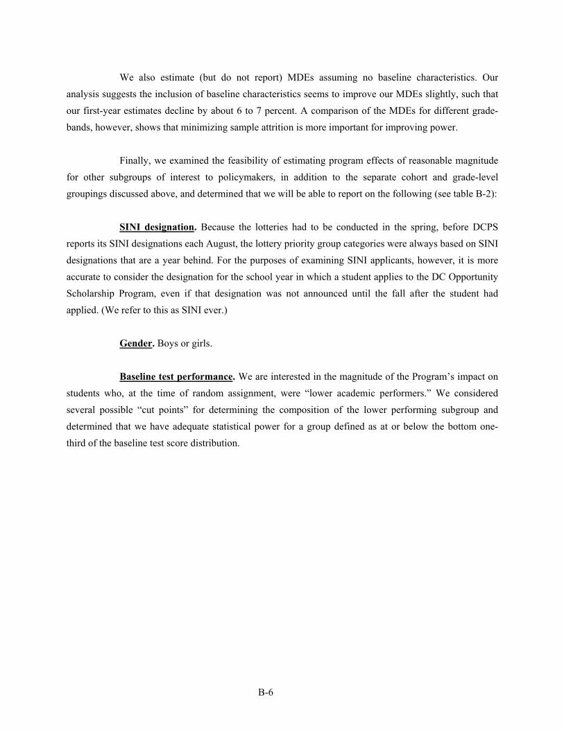
B-6
We also estimate (but do not report) MDEs assuming no baseline characteristics. Our analysis suggests the inclusion of baseline characteristics seems to improve our MDEs slightly, such that our first-year estimates decline by about 6 to 7 percent. A comparison of the MDEs for different grade-bands, however, shows that minimizing sample attrition is more important for improving power.
Finally, we examined the feasibility of estimating program effects of reasonable magnitude for other subgroups of interest to policymakers, in addition to the separate cohort and grade-level groupings discussed above, and determined that we will be able to report on the following (see table B-2):
SINI designation. Because the lotteries had to be conducted in the spring, before DCPS
reports its SINI designations each August, the lottery priority group categories were always based on SINI designations that are a year behind. For the purposes of examining SINI applicants, however, it is more accurate to consider the designation for the school year in which a student applies to the DC Opportunity Scholarship Program, even if that designation was not announced until the fall after the student had applied. (We refer to this as SINI ever.)
Gender. Boys or girls. Baseline test performance. We are interested in the magnitude of the Program’s impact on
students who, at the time of random assignment, were “lower academic performers.” We considered several possible “cut points” for determining the composition of the lower performing subgroup and determined that we have adequate statistical power for a group defined as at or below the bottom one-third of the baseline test score distribution.
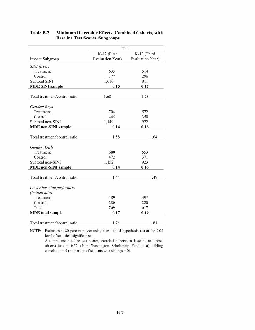
B-7
Table B-2. Minimum Detectable Effects, Combined Cohorts, with Baseline Test Scores, Subgroups
Total
Impact Subgroup K-12 (First
Evaluation Year) K-12 (Third
Evaluation Year)
SINI (Ever) Treatment 633 514 Control 377 296
Subtotal SINI 1,010 811 MDE SINI sample 0.15 0.17 Total treatment/control ratio 1.68 1.73 Gender: Boys
Treatment 704 572 Control 445 350
Subtotal non-SINI 1,149 922 MDE non-SINI sample 0.14 0.16 Total treatment/control ratio 1.58 1.64 Gender: Girls
Treatment 680 553 Control 472 371
Subtotal non-SINI 1,152 923 MDE non-SINI sample 0.14 0.16 Total treatment/control ratio 1.44 1.49 Lower baseline performers (bottom third)
Treatment 489 397 Control 280 220 Total 769 617
MDE total sample 0.17 0.19 Total treatment/control ratio 1.74 1.81
NOTE: Estimates at 80 percent power using a two-tailed hypothesis test at the 0.05 level of statistical significance. Assumptions: baseline test scores, correlation between baseline and post-observations = 0.57 (from Washington Scholarship Fund data); sibling correlation = 0 (proportion of students with siblings = 0).
C-1
Appendix C Treatment of Observations with Incomplete Test Score Data
Like most norm-referenced standardized tests, the SAT-9 includes subtests within the reading and math domains in most grades, e.g., the Reading Comprehension subtest is one component of the reading test battery. Ideally, students complete each subtest within a given domain, and their total or composite score for that domain is the average of their performance on the various subtests. The composite score is superior to any specific subtest score as a measure of achievement in reading or math because it represents a more comprehensive gauge of mastery of domain skills and content and also draws upon more test items in calculating the achievement score. When available, composite scores for a domain are preferred to subtest scores alone.
The SAT-9 is designed to provide relatively intensive testing of the various aspects of
reading ability for first and second graders. During the baseline test administrations, this posed a special problem for first graders, many of whom struggled to complete both of the reading subtests, and their parents, who were required to remain at the testing event longer than the parents of students in other grades. As a result, the decision was made to only administer the extensive Reading Comprehension subtest to all first graders at outcome testing and to use that subtest score as the measure of reading outcomes for those students. Other students provided some, but not all, outcome subtest scores within the two domains because they either missed or skipped entire subtests. This included 77 students of various grades (besides first) in reading, and 59 students in grades K-12 in math.1
Before deciding whether to include or exclude respondents who contributed only subtest
scores during outcome data collection, an analysis was conducted to determine how closely subtest reading and math scores correlated with composite scores for the over 1,600 respondents for whom both subtest and composite scores were available. The correlations between subtest and composite scores within particular domains and grades were very strong, ranging from a low of r =.79 to a high of r = .92.2 Given such high levels of correlations, and consistent with the principle of bringing as many observations as possible to the test score impact analysis, a decision was made to substitute subtest scores for the composite scores in the 136 cases where only the subtest scores were available. Those cases were
1 In grades 9-12, the SAT-9 includes only a single mathematics test with no subsections. 2 Figures are for bivariate correlations using Pearson’s R.
C-2
considered respondents for the purposes of calculating the test score non-response weights and were therefore included in the test score impact analysis.
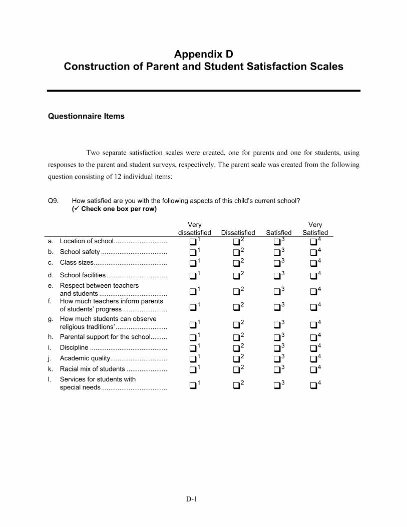
D-1
Appendix D Construction of Parent and Student Satisfaction Scales
Questionnaire Items
Two separate satisfaction scales were created, one for parents and one for students, using
responses to the parent and student surveys, respectively. The parent scale was created from the following question consisting of 12 individual items: Q9. How satisfied are you with the following aspects of this child’s current school?
( Check one box per row) Very
dissatisfied Dissatisfied Satisfied Very
Satisfied a. Location of school............................. 1 2 3 4 b. School safety .................................... 1 2 3 4 c. Class sizes........................................ 1 2 3 4 d. School facilities ................................. 1 2 3 4 e. Respect between teachers
and students ..................................... 1 2 3 4
f. How much teachers inform parents of students’ progress ........................
1 2 3 4 g. How much students can observe
religious traditions’ ............................ 1 2 3 4
h. Parental support for the school......... 1 2 3 4 i. Discipline .......................................... 1 2 3 4 j. Academic quality............................... 1 2 3 4 k. Racial mix of students ...................... 1 2 3 4 l. Services for students with
special needs.................................... 1 2 3 4
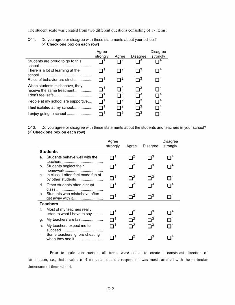
D-2
The student scale was created from two different questions consisting of 17 items: Q11. Do you agree or disagree with these statements about your school?
( Check one box on each row)
Q13. Do you agree or disagree with these statements about the students and teachers in your school? ( Check one box on each row)
Agree strongly Agree Disagree
Disagree strongly
Students a. Students behave well with the
teachers........................................1 2 3 4
b. Students neglect their homework.....................................
1 2 3 4
c. In class, I often feel made fun of by other students..........................
1 2 3 4 d. Other students often disrupt
class .............................................1 2 3 4
e. Students who misbehave often get away with it .............................
1 2 3 4 Teachers f. Most of my teachers really
listen to what I have to say ...........1 2 3 4
g. My teachers are fair...................... 1 2 3 4 h. My teachers expect me to
succeed ........................................1 2 3 4
i. Some teachers ignore cheating when they see it ...........................
1 2 3 4
Prior to scale construction, all items were coded to create a consistent direction of
satisfaction, i.e., that a value of 4 indicated that the respondent was most satisfied with the particular dimension of their school.
Agree strongly Agree Disagree
Disagree strongly
Students are proud to go to this school ..................................................
1 2 3 4
There is a lot of learning at the school ..................................................
1 2 3 4
Rules of behavior are strict ................. 1 2 3 4 When students misbehave, they receive the same treatment.................
1 2 3 4 I don’t feel safe.................................... 1 2 3 4 People at my school are supportive.... 1 2 3 4 I feel isolated at my school.................. 1 2 3 4 I enjoy going to school ........................ 1 2 3 4

D-3
Scale Development and Scoring
The two scales were developed, and scores assigned to individual parents and students, using a statistical procedure called maximum likelihood Item Response Theory (IRT) (see Hambleton et al., 1991). IRT has gained increasing attention in the development of standardized academic tests and, most recently, in the development of scales measuring a wide variety of “subjective traits” such as satisfaction with treatment and individual perceptions of health status and overall quality of life.
The basic idea of IRT is to model a relationship between a hypothesized underlying trait or
construct, which is unobserved, and an individual’s responses to a set of survey questions or items on a test. Common educational examples are a student’s reading and math ability as measured by an achievement test. In the current situation, the underlying trait of interest is the student’s or parent’s “satisfaction” with the child’s school. The results of the IRT analysis can be used to determine the extent to which the items included in the scale (or test) are good measures of the underlying construct, and how well the items “hang together” (show common relationships) to characterize the underlying, and unobserved, construct.
In IRT models, the underlying trait or construct of interest (e.g., an individual’s reading
ability) is designated by theta (θ). Individuals with higher levels of θ have a higher probability of getting a particular test item correct or, in our case, a higher probability of agreeing with a particular item in the satisfaction scale, than do individuals with lower levels of θ. The modeled relationship between θ and the individual test or questionnaire items is typically based on 2-parameter logistic function: (1) the first parameter is the item difficulty, which captures individual differences in their ability to get an item correct (or in their satisfaction), and (2) the second parameter is the slope, or discrimination, parameter, which captures how well a particular item differentiates between individuals on the underlying construct or trait. In other words, the IRT model estimates the probability of getting a particular item correct on a test (or agreeing with a statement on an attitude scale) conditional on an individual’s underlying trait level, i.e., the higher a person’s trait level, the greater the probability that the person will agree with the item or provide a correct answer. For example, if the following statement is presented, “Students behave well with the teachers.” Then students with higher levels of satisfaction (our θ in this example) will have higher probabilities for agreeing with this statement.
More traditional methods of creating scales often involve just counts of individual item-level
responses, i.e., this approach assumes that each item is equally related to the underlying trait. IRT, on the other hand, uses all of the available information contained in an individual’s responses to all of the test or survey questions and uses the difficulty and discrimination parameters to estimate an individual’s test or
D-4
scale score. As a result, two individuals can have the same summed score (e.g., the same number of correct test items), but they may have very different IRT scores if they had a different pattern of responses. For example, if this were a test of academic ability one student might answer more of the highly discriminating and difficult items than another student and would receive a higher IRT-derived score than another student who answered the same number of items but scored correctly on items with lower difficulty.
Another important advantage of IRT models is that they can produce reliable scale estimates
even when an individual fails to respond to particular items, i.e., the model yields the same estimate of the individual’s score regardless of missing data.
Final Notes
For this analysis a single parent satisfaction scale and a single student satisfaction scale were
developed, and each scale exhibited high reliability—the Cronbach’s Alphas were 0.938 and 0.814, respectively.
Our initial decision to create a single student and parent satisfaction scale was based on the
need to have a single comparable outcome measure for all students and parents that could be used in the pooled analyses described in the body of this report. Subsequent analysis, conducted after the completion of this report, has indicated a relationship between student’s grade in school and satisfaction. Parent and student satisfaction in general decrease as students move through junior high and high school.
To examine the possible effect of grade differences in the development and scoring of the
satisfaction scales, multiple group IRT scaling was conducted using group-specific Bayesian priors, i.e., the student’s grade was taken into account in the scoring of both the student and parent scales. The new results are somewhat more sensitive to grade-level differences (i.e., they are slightly more reliable and efficient) but the data likelihoods and posterior distributions are virtually identical. The original scales have such high reliabilities that accounting for grade level in the prior distributions yields almost identical results.
We will explore this issue more completely for subsequent reports; however, the general
response patterns were so strong, as evidenced by high ratings of Cronbach’s Alpha, that the analytic results reported here are unlikely to be meaningfully different with the more nuanced satisfaction scales.
E-1
Appendix E Imputation for Missing Baseline Covariates
One difficulty that arose regarding the baseline data was the extent to which data were missing (table 2-3 in chapter 2). Although some important baseline covariates (e.g., family income, grade, race, and gender) were available for all students, other baseline covariates contained some missing values. Importantly, nearly 20 percent of math scores and 29 percent of reading scores were not obtained at baseline.1 To deal with this occurrence, missing baseline data were imputed by fitting stepwise models to each covariate using all of the available baseline covariates as potential predictors. Predicted values were then generated, and imputation was done using a “nearest neighbor” procedure in which a “donor” was found for each “recipient” in a way that minimized the difference between the predicted value for the recipient and the actual value for the donor across all potential donors.2 For example, if a particular student was missing a value for the total number of children in the student’s household, a regression estimation predicted the likely number of children in the student’s household (e.g., 2.8) based on all known characteristics of the student, and another student in the study was located with a known value (e.g., 3) for number of children in the household that closely matched the value the data predicted the student might have. That donor student’s value was then imputed as the recipient’s value for that characteristic.3
1 In some of these cases, students did not come for the required baseline testing. In other cases, they attended the testing but did
not attempt to answer enough questions on one or more of the subsections of the test to be assigned a valid test score. 2 The stepwise regressions and imputations that made up the imputation procedure were done in an iterative cycle, in that
‘current’ imputations were used in fitting the stepwise model, and then that stepwise model was used to generate a new set of imputations. This imputation-regression-imputation cycle went through the set of baseline covariates in a cyclical sequence, and this was continued until convergence resulted (i.e., no change in imputations or model fits between cycles). To initiate the procedure (i.e., to get the first set of imputations) an initial set of imputations was computed via a simple hot deck procedure. The final result of this algorithm was an efficient set of imputations that respected the underlying patterns in the data as was picked up by the stepwise regression procedures, while providing a set of imputations with distributional patterns similar to those of the real values.
3 For continuous variables (e.g., baseline score), a residual was taken from a hot deck procedure (a random draw from all residuals from the model), and added to the predicted value from the recipient.
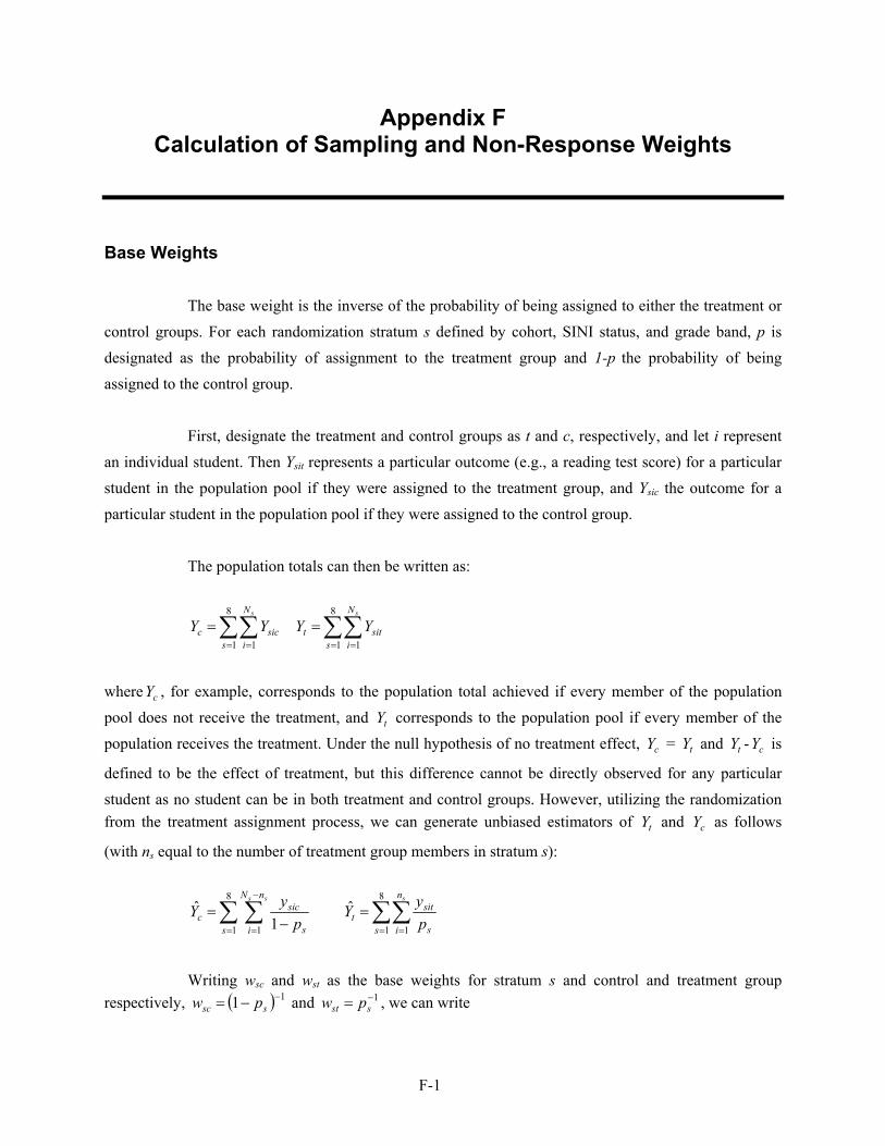
F-1
Appendix F Calculation of Sampling and Non-Response Weights
Base Weights
The base weight is the inverse of the probability of being assigned to either the treatment or control groups. For each randomization stratum s defined by cohort, SINI status, and grade band, p is designated as the probability of assignment to the treatment group and 1-p the probability of being assigned to the control group.
First, designate the treatment and control groups as t and c, respectively, and let i represent
an individual student. Then Ysit represents a particular outcome (e.g., a reading test score) for a particular student in the population pool if they were assigned to the treatment group, and Ysic the outcome for a particular student in the population pool if they were assigned to the control group.
The population totals can then be written as:
∑∑∑∑= == =
==8
1 1
8
1 1
s
N
isitt
s
N
isicc
ss
YYYY
where cY , for example, corresponds to the population total achieved if every member of the population pool does not receive the treatment, and tY corresponds to the population pool if every member of the population receives the treatment. Under the null hypothesis of no treatment effect, cY = tY and tY - cY is
defined to be the effect of treatment, but this difference cannot be directly observed for any particular student as no student can be in both treatment and control groups. However, utilizing the randomization from the treatment assignment process, we can generate unbiased estimators of tY and cY as follows
(with ns equal to the number of treatment group members in stratum s):
∑∑∑ ∑= ==
−
=
=−
=8
1 1
8
1 1
ˆ 1
ˆs
n
i s
sitt
s
nN
i s
sicc
sss
pyY
pyY
Writing wsc and wst as the base weights for stratum s and control and treatment group
respectively, ( ) 11 −−= ssc pw and 1−= sst pw , we can write
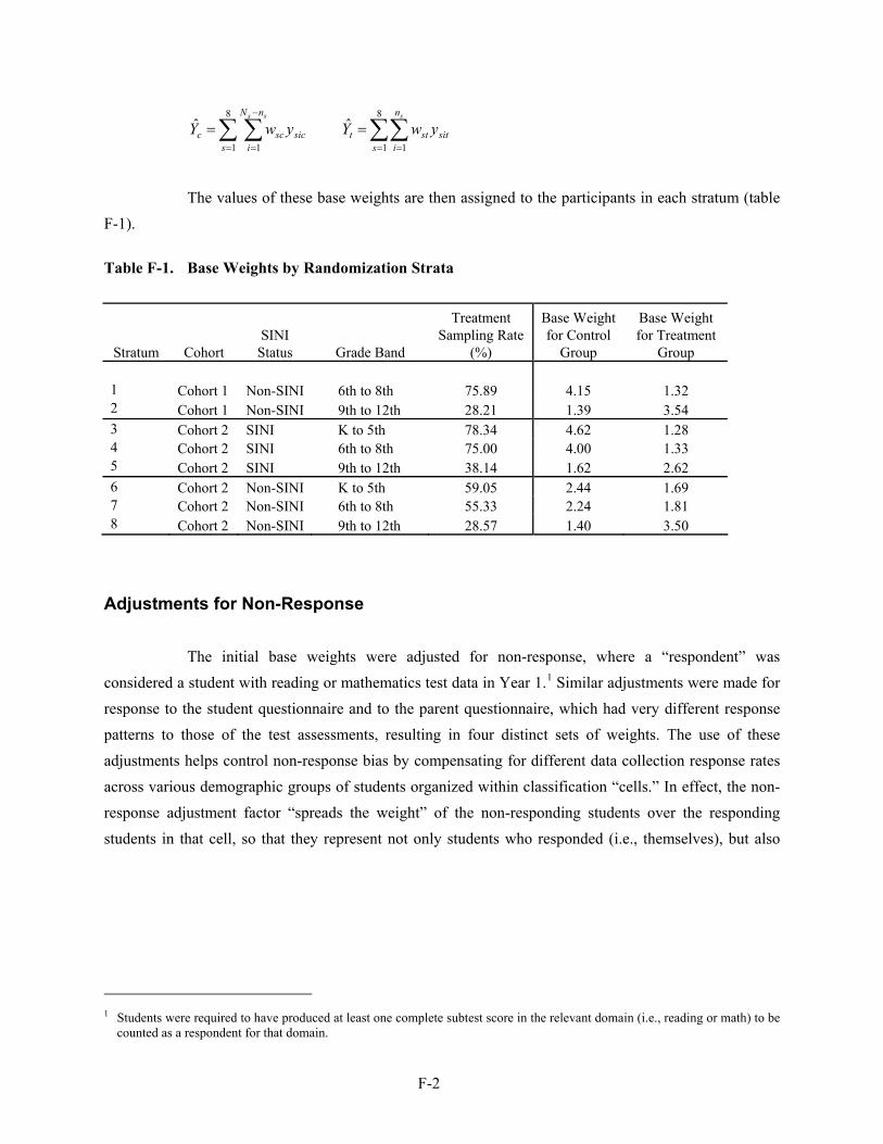
F-2
∑∑∑ ∑= ==
−
=
==8
1 1
8
1 1
ˆ ˆs
n
isitstt
s
nN
isicscc
sss
ywYywY
The values of these base weights are then assigned to the participants in each stratum (table
F-1).
Table F-1. Base Weights by Randomization Strata
Stratum Cohort SINI
Status Grade Band
Treatment Sampling Rate
(%)
Base Weight for Control
Group
Base Weight for Treatment
Group 1 Cohort 1 Non-SINI 6th to 8th 75.89 4.15 1.32 2 Cohort 1 Non-SINI 9th to 12th 28.21 1.39 3.54 3 Cohort 2 SINI K to 5th 78.34 4.62 1.28 4 Cohort 2 SINI 6th to 8th 75.00 4.00 1.33 5 Cohort 2 SINI 9th to 12th 38.14 1.62 2.62 6 Cohort 2 Non-SINI K to 5th 59.05 2.44 1.69 7 Cohort 2 Non-SINI 6th to 8th 55.33 2.24 1.81 8 Cohort 2 Non-SINI 9th to 12th 28.57 1.40 3.50
Adjustments for Non-Response
The initial base weights were adjusted for non-response, where a “respondent” was considered a student with reading or mathematics test data in Year 1.1 Similar adjustments were made for response to the student questionnaire and to the parent questionnaire, which had very different response patterns to those of the test assessments, resulting in four distinct sets of weights. The use of these adjustments helps control non-response bias by compensating for different data collection response rates across various demographic groups of students organized within classification “cells.” In effect, the non-response adjustment factor “spreads the weight” of the non-responding students over the responding students in that cell, so that they represent not only students who responded (i.e., themselves), but also
1 Students were required to have produced at least one complete subtest score in the relevant domain (i.e., reading or math) to be
counted as a respondent for that domain.
F-3
students who were like them in relevant ways but did not respond to outcome data collection.2 This maintains the same mix of the impact sample across classification cells as would have been present had there been no non-response (see Howell and Peterson et al., 2002, pp. 209-216; U.S. Department of Health and Human Services, 2005). As a last step, the non-response-adjusted base weights were trimmed. This is done to prevent extremely large weights from unduly inflating the estimated variances and thus reducing the precision of the impact estimates.3
Even with the weighting protocol to adjust for non-response described above, however, there
was a large differential between the response rates of the two experimental groups, which could undermine their comparability and therefore bias the impact analysis. After four invitations to attend data collection events, the evaluation team had obtained responses from nearly 80 percent of the treatment group but only about 60 percent of the control group.
Recently, a new technique was developed to help reduce non-response bias in longitudinal
impact analyses. Non-response subsampling is a strategy to reduce the differences between the characteristics of baseline and outcome samples by way of random sampling and non-response conversion. After the regular period of outcome data collection is over, a subsample of non-respondents is drawn and subjected to intensive efforts at non-response conversion. If initial non-response was significantly higher in one experimental group compared with the other, as was the case in this evaluation, then the subsample can be drawn exclusively from the underresponded group (e.g., controls). Each initial non-respondent who converts to a respondent by providing outcome data counts as one more respondent for purposes of the “actual” response rate but counts as 1/sampling rate (r) respondents for purposes of the “effective” response rate. Through a simple weighting algorithm, the random sampling permits the respondent to also “stand in” for members of the initial non-respondent group who were not selected for the subsample but who presumably would have converted to respondent status if they had been selected to
2 To determine the factors used to create the non-response adjustment cells, both logistic regression (with response or not as the
dependent variable) and a software package called CHAID (Chi-squared Automatic Interaction Detector) were used to determine which of the available baseline variables were correlated with the propensity to respond. The available baseline variables from which predictors of response propensity were drawn included family income, mother’s job status, mother’s education, disability status of the child, race, grade, gender, and baseline test score data (both reading and math). Stepwise logistic regression was first used to select a set of characteristics generally predictive of response (using the SAS procedure PROC LOGISTIC with a 20 percent level of significance entry cutoff). These stepwise procedures were done separately within each of the eight sampling strata. The CHAID program (now a part of the SPSS statistical software package) was then used to define a set of cells with differing response rates within each sampling stratum, using the set of characteristics for the sampling stratum coming from the PROC LOGISTIC models. Cells with fewer than six observations were not allowed. The non-response cells nested within the sampling strata and within treatment status. The non-response adjustment for each respondent in the cell was equal to the reciprocal of the base-weighted response rate within the cell.
3 The trimming rule was that any weights that were larger than 4.5 times the median weight (with medians computed separately within the treatment and control groups) were trimmed back to be equal to 4.5 times the median weight. This procedure affected only a very small number of cases. Such trimming is standard procedure and is done for example as a matter of course in the National Assessment of Educational Progress (NAEP) assessment sample weighting.
F-4
receive the intense effects and incentives that were the conversion “treatment.” In other words, the proportion of subsampled non-respondents that converts represents themselves as well as the same proportion of nonsampled non-respondents.
This technique was applied for the spring 2006 data collection to increase the outcome
response rates for the control group and reduce the response rate differential across the experimental subgroups. The initial data gathering effort was followed by a targeted intensive recruitment of control group initial non-responders. A random sample of 96 of the 235 control group non-respondents (41 percent) was drawn, and the selected participants were offered a larger turnout incentive and greater flexibility and convenience in an attempt to “convert” as many as possible from non-respondent to respondent status. A total of 42 initial non-respondents were converted to respondents as a result of this effort (44 percent). These “converted” control group cases were more heavily weighted4 to account for the complementary set of initial non-respondents who were not randomly selected for targeted conversion efforts but who would have responded if they had been targeted (see Kling, Ludwig, and Katz, 2005; Sanbonmatsu, Kling, Duncan, and Brooks-Gunn, 2006).5 As a result of implementing this approach, the combined cohort control group response rate increased to an effective rate of 74 percent, and the treatment-control response differential decreased to 5 percentage points (table F-2).
The final student-level weights for the analysis were equal to: Wi = (1/pi) * (Xi) * (NRj) * (TRi),
where pi is the probability of selection to treatment or control for student i, Xi is the special factor for control initial nonrespondents (with Xi equal to 2.45 for this set, and equal to 1 otherwise), NRj is the non-response adjustment (the reciprocal of the response rate) for the classification cell to which student i belongs, and TRi is the trimming adjustment (usually equal to 1, but in some cases equal to 4.5 times median cutoff divided by the untrimmed weight).
4 The final weighting factor for the spring 2006 data collection was 2.45 (the reciprocal of 0.4085). 5 For example, the Moving to Opportunity Section 8 housing voucher experimental evaluation obtained an initial year 1
response rate of 78 percent. Evaluators then drew a random sample of 30 percent of the initial non-responders and subjected them to intense recruitment efforts that resulted in nearly half of them responding, thereby increasing their response rate to 81 percent. The evaluators then assumed that the second-wave respondents were similar to the half of the larger non-respondent group that they did not pursue aggressively and thus estimate and report an “effective response rate” of 90 percent, even though actual data were obtained for only 81 percent of the respondents.
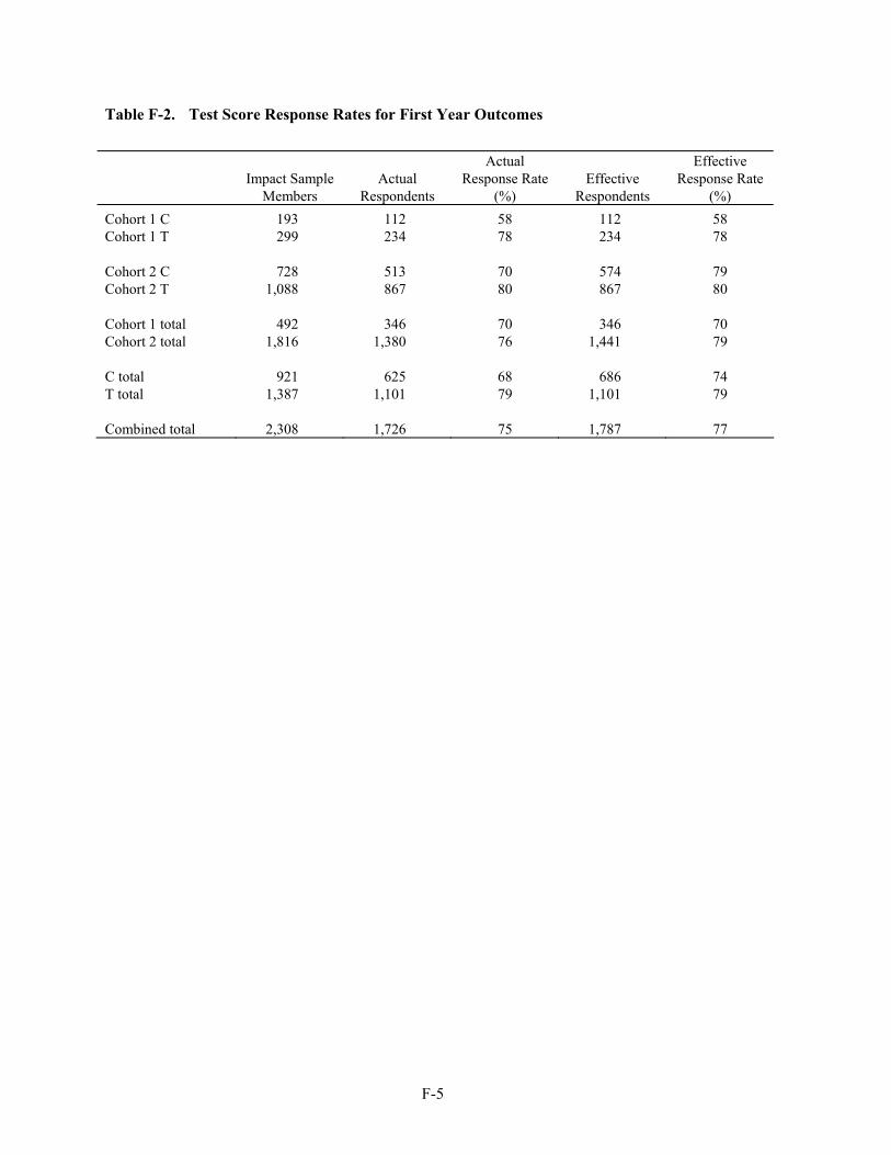
F-5
Table F-2. Test Score Response Rates for First Year Outcomes
Impact Sample
Members Actual
Respondents
Actual Response Rate
(%) Effective
Respondents
Effective Response Rate
(%) Cohort 1 C 193 112 58 112 58 Cohort 1 T 299 234 78 234 78 Cohort 2 C 728 513 70 574 79 Cohort 2 T 1,088 867 80 867 80 Cohort 1 total 492 346 70 346 70 Cohort 2 total 1,816 1,380 76 1,441 79 C total 921 625 68 686 74 T total 1,387 1,101 79 1,101 79 Combined total 2,308 1,726 75 1,787 77
G-1
Appendix G Additional Detail on the Analytic Methods for Estimating the
Impact of Using a Scholarship and of Attending a Private School
Impact of Using a Scholarship
This method uses the original comparison of all treatment group members to all control group members but re-scales it to account for the fact that a known fraction of the treatment group members did not actually avail themselves of the treatment. Any treatment impact observed through the intent-to-treat (ITT) is reasonably assumed to have been generated entirely by the component of the treatment group that actually used the scholarships and not by the component that declined to use them (see Bloom, 1984, pp. 225-246).1
In effect, the overall impact of the treatment on all students is simply a weighted average of
the impact on users and the impact on the decliners: Impact (on all students) = P (impact on users) + Q (impact on decliners)
where P is the number of users in the treatment group and Q is the number of decliners in the treatment group. If the assumption of zero impact on the decliners is incorporated into this equation, one gets the following expression:
Impact (on all students) = P (impact on users) + 0
{Impact (on all students)}/P = (impact on users)
1 This assumption alone—the presumption that the decliners remain unaffected by their assignment to the treatment group—
makes it possible to translate the measured effect of the Opportunity Scholarship Program (OSP) on the entire treatment group (which the experimental design provides directly as described above) as a way to assess the average effect of the program on just the users. It does not matter what the average effect would have been on the decliners had they participated. Nor does it matter whether decliners have different outcomes than users due to “selection” or pre-existing differences. Specifically, if the original experimental comparison of average outcomes between all treatment group members and all control group members is not biased by systematic differences between these two randomly generated groups at baseline, the simple rescaling of the original estimate cannot be biased. This theorem, based solely on the assumption of zero impacts on the decliners, provides a broadly accepted basis for the now almost universal practice of reporting impact estimates for users-only along with the all-intervention-group impact findings.
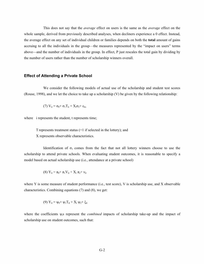
G-2
This does not say that the average effect on users is the same as the average effect on the whole sample, derived from previously described analyses, when decliners experience a 0 effect. Instead, the average effect on any set of individual children or families depends on both the total amount of gains accruing to all the individuals in the group—the measures represented by the “impact on users” terms above—and the number of individuals in the group. In effect, P just rescales the total gain by dividing by the number of users rather than the number of scholarship winners overall.
Effect of Attending a Private School
We consider the following models of actual use of the scholarship and student test scores (Rouse, 1998), and we let the choice to take up a scholarship (V) be given by the following relationship:
(7) Vit = σ0+ σ1Tit + Xiσ2+ εit,
where i represents the student, t represents time; T represents treatment status (=1 if selected in the lottery); and
X represents observable characteristics. Identification of σ1 comes from the fact that not all lottery winners choose to use the
scholarship to attend private schools. When evaluating student outcomes, it is reasonable to specify a model based on actual scholarship use (i.e., attendance at a private school)
(8) Yit = π0+ π1Vit + Xi π2+ νit
where Y is some measure of student performance (i.e., test score), V is scholarship use, and X observable characteristics. Combining equations (7) and (8), we get:
(9) Yit = ψ0+ ψ1Tit + Xi ψ2+ ξit
where the coefficients ψis represent the combined impacts of scholarship take-up and the impact of scholarship use on student outcomes, such that:
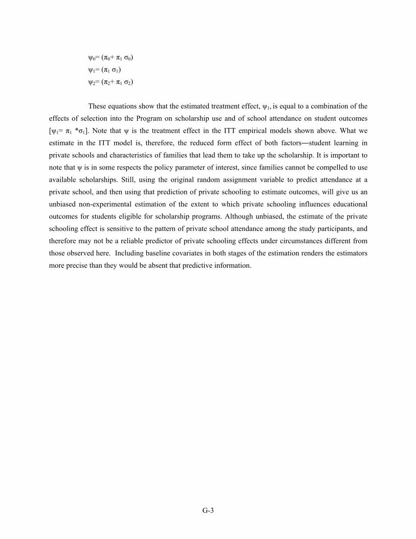
G-3
ψ0= (π0+ π1 σ0) ψ1= (π1 σ1) ψ2= (π2+ π1 σ2)
These equations show that the estimated treatment effect, ψ1, is equal to a combination of the
effects of selection into the Program on scholarship use and of school attendance on student outcomes [ψ1= π1 *σ1]. Note that ψ is the treatment effect in the ITT empirical models shown above. What we estimate in the ITT model is, therefore, the reduced form effect of both factors―student learning in private schools and characteristics of families that lead them to take up the scholarship. It is important to note that ψ is in some respects the policy parameter of interest, since families cannot be compelled to use available scholarships. Still, using the original random assignment variable to predict attendance at a private school, and then using that prediction of private schooling to estimate outcomes, will give us an unbiased non-experimental estimation of the extent to which private schooling influences educational outcomes for students eligible for scholarship programs. Although unbiased, the estimate of the private schooling effect is sensitive to the pattern of private school attendance among the study participants, and therefore may not be a reliable predictor of private schooling effects under circumstances different from those observed here. Including baseline covariates in both stages of the estimation renders the estimators more precise than they would be absent that predictive information.
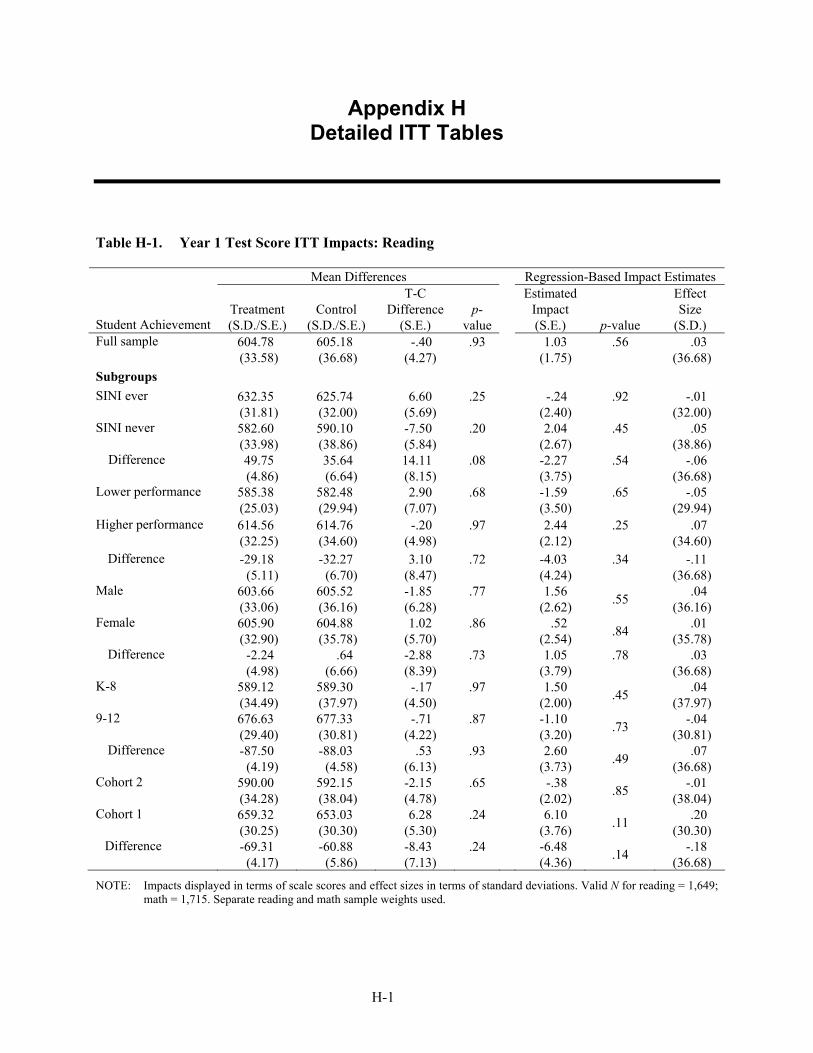
H-1
Appendix H Detailed ITT Tables
Table H-1. Year 1 Test Score ITT Impacts: Reading
Mean Differences Regression-Based Impact Estimates
Student Achievement Treatment (S.D./S.E.)
Control (S.D./S.E.)
T-C Difference
(S.E.) p-
value
Estimated Impact (S.E.) p-value
Effect Size
(S.D.) Full sample 604.78
(33.58) 605.18 (36.68)
-.40 (4.27)
.93
1.03 (1.75)
.56 .03 (36.68)
Subgroups SINI ever 632.35
(31.81) 625.74 (32.00)
6.60 (5.69)
.25
-.24 (2.40)
.92 -.01 (32.00)
SINI never 582.60 (33.98)
590.10 (38.86)
-7.50 (5.84)
.20
2.04 (2.67)
.45 .05 (38.86)
Difference 49.75 (4.86)
35.64 (6.64)
14.11 (8.15)
.08
-2.27 (3.75)
.54 -.06 (36.68)
Lower performance 585.38 (25.03)
582.48 (29.94)
2.90 (7.07)
.68
-1.59 (3.50)
.65 -.05 (29.94)
Higher performance 614.56 (32.25)
614.76 (34.60)
-.20 (4.98)
.97
2.44 (2.12)
.25 .07 (34.60)
Difference -29.18 (5.11)
-32.27 (6.70)
3.10 (8.47)
.72
-4.03 (4.24)
.34 -.11 (36.68)
Male 603.66 (33.06)
605.52 (36.16)
-1.85 (6.28)
.77
1.56 (2.62) .55 .04
(36.16) Female 605.90
(32.90) 604.88 (35.78)
1.02 (5.70)
.86
.52 (2.54) .84 .01
(35.78) Difference -2.24
(4.98) .64
(6.66) -2.88 (8.39)
.73
1.05 (3.79)
.78 .03 (36.68)
K-8 589.12 (34.49)
589.30 (37.97)
-.17 (4.50)
.97
1.50 (2.00) .45 .04
(37.97) 9-12 676.63
(29.40) 677.33 (30.81)
-.71 (4.22)
.87
-1.10 (3.20) .73 -.04
(30.81) Difference -87.50
(4.19) -88.03
(4.58) .53
(6.13) .93
2.60
(3.73) .49 .07 (36.68)
Cohort 2 590.00 (34.28)
592.15 (38.04)
-2.15 (4.78)
.65
-.38 (2.02) .85 -.01
(38.04) Cohort 1 659.32
(30.25) 653.03 (30.30)
6.28 (5.30)
.24
6.10 (3.76) .11 .20
(30.30) Difference -69.31
(4.17) -60.88
(5.86) -8.43 (7.13)
.24
-6.48 (4.36) .14 -.18
(36.68)
NOTE: Impacts displayed in terms of scale scores and effect sizes in terms of standard deviations. Valid N for reading = 1,649; math = 1,715. Separate reading and math sample weights used.
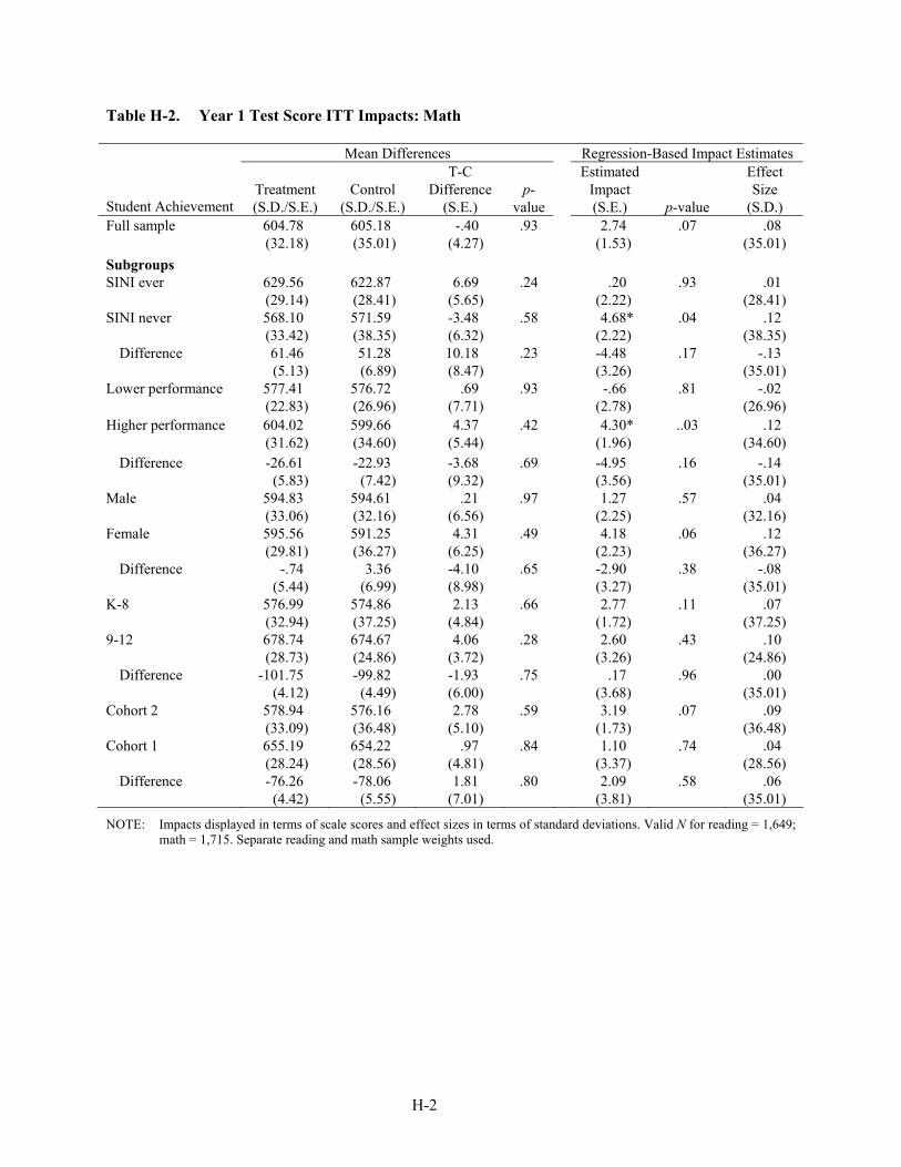
H-2
Table H-2. Year 1 Test Score ITT Impacts: Math
Mean Differences Regression-Based Impact Estimates
Student Achievement Treatment (S.D./S.E.)
Control (S.D./S.E.)
T-C Difference
(S.E.) p-
value
Estimated Impact (S.E.) p-value
Effect Size
(S.D.) Full sample 604.78
(32.18) 605.18 (35.01)
-.40 (4.27)
.93
2.74 (1.53)
.07 .08 (35.01)
Subgroups SINI ever 629.56
(29.14) 622.87 (28.41)
6.69 (5.65)
.24
.20 (2.22)
.93 .01 (28.41)
SINI never 568.10 (33.42)
571.59 (38.35)
-3.48 (6.32)
.58
4.68* (2.22)
.04 .12 (38.35)
Difference 61.46 (5.13)
51.28 (6.89)
10.18 (8.47)
.23
-4.48 (3.26)
.17 -.13 (35.01)
Lower performance 577.41 (22.83)
576.72 (26.96)
.69 (7.71)
.93
-.66 (2.78)
.81 -.02 (26.96)
Higher performance 604.02 (31.62)
599.66 (34.60)
4.37 (5.44)
.42
4.30* (1.96)
..03 .12 (34.60)
Difference -26.61 (5.83)
-22.93 (7.42)
-3.68 (9.32)
.69
-4.95 (3.56)
.16 -.14 (35.01)
Male 594.83 (33.06)
594.61 (32.16)
.21 (6.56)
.97
1.27 (2.25)
.57 .04 (32.16)
Female 595.56 (29.81)
591.25 (36.27)
4.31 (6.25)
.49
4.18 (2.23)
.06 .12 (36.27)
Difference -.74 (5.44)
3.36 (6.99)
-4.10 (8.98)
.65
-2.90 (3.27)
.38 -.08 (35.01)
K-8 576.99 (32.94)
574.86 (37.25)
2.13 (4.84)
.66
2.77 (1.72)
.11 .07 (37.25)
9-12 678.74 (28.73)
674.67 (24.86)
4.06 (3.72)
.28
2.60 (3.26)
.43 .10 (24.86)
Difference -101.75 (4.12)
-99.82 (4.49)
-1.93 (6.00)
.75
.17 (3.68)
.96 .00 (35.01)
Cohort 2 578.94 (33.09)
576.16 (36.48)
2.78 (5.10)
.59
3.19 (1.73)
.07 .09 (36.48)
Cohort 1 655.19 (28.24)
654.22 (28.56)
.97 (4.81)
.84
1.10 (3.37)
.74 .04 (28.56)
Difference -76.26 (4.42)
-78.06 (5.55)
1.81 (7.01)
.80
2.09 (3.81)
.58 .06 (35.01)
NOTE: Impacts displayed in terms of scale scores and effect sizes in terms of standard deviations. Valid N for reading = 1,649; math = 1,715. Separate reading and math sample weights used.
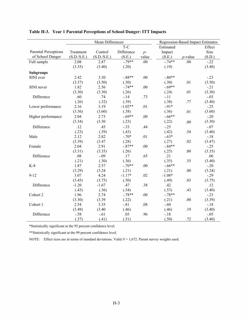
H-3
Table H-3. Year 1 Parental Perceptions of School Danger: ITT Impacts
Mean Differences Regression-Based Impact Estimates
Parental Perceptions of School Danger
Treatment (S.D./S.E.)
Control (S.D./S.E.)
T-C Difference
(S.E.) p-
value
Estimated Impact (S.E.) p-value
Effect Size
(S.D.) Full sample 2.08
(3.35) 2.87
(3.40) -.79** (.20)
.00
-.74** (.19)
.00 -.22 (3.40)
Subgroups SINI ever 2.42
(3.37) 3.30
(3.50) -.88** (.30)
.00
-.80** (.30) .01
-.23 (3.50)
SINI never 1.82 (3.30)
2.56 (3.30)
-.74** (.26)
.00
-.69** (.24) .01
-.21 (3.30)
Difference .60 (.26)
.74 (.32)
-.14 (.39)
.73
-.11 (.38) .77
-.03 (3.40)
Lower performance 2.16 (3.36)
3.19 (3.60)
-1.02** (.38)
.01
-.91* (.36) .01
-.25 (3.60)
Higher performance 2.04 (3.34)
2.73 (3.30
-.69** (.23)
.00
-.66** (.22) .00
-.20 (3.30)
Difference .12 (.23)
.45 (.39)
-.33 (.43)
.44
-.25 (.42) .54
-.07 (3.40)
Male 2.12 (3.39)
2.82 (3.47
-.70* (.28)
.01
-.63* (.27) .02
-.18 (3.47)
Female 2.04 (3.31)
2.91 (3.35)
-.87** (.26)
.00
-.84** (.25) .00
-.25 (3.35)
Difference .08 (.21)
-.09 (.30)
.17 (.36)
.65
.21 (.35) .55
.06 (3.40)
K-8 1.87 (3.29)
2.57 (3.24
-.70** (.21)
.00
-.66** (.21) .00
-.20 (3.24)
9-12 3.07 (3.45)
4.24 (3.75)
-1.17* (.50)
.02
-1.08* (.49) .03
-.29 (3.75)
Difference -1.20 (.43)
-1.67 (.36)
.47 (.54)
.38
.42 (.53) .43
.12 (3.40)
Cohort 2 1.96 (3.30)
2.74 (3.39
-.78** (.22)
.00
-.78** (.21) .00
-.23 (3.39)
Cohort 1 2.54 (3.49)
3.35 (3.40
-.81 (.46)
.08
-.60 (.46) .19
-.18 (3.40)
Difference -.58 (.37)
-.61 (.41)
.03 (.51)
.96
-.18 (.50) .72
-.05 (3.40)
*Statistically significant at the 95 percent confidence level.
**Statistically significant at the 99 percent confidence level.
NOTE: Effect sizes are in terms of standard deviations. Valid N = 1,672. Parent survey weights used.
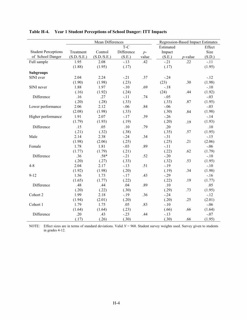
H-4
Table H-4. Year 1 Student Perceptions of School Danger: ITT Impacts
Mean Differences Regression-Based Impact Estimates
Student Perceptions of School Danger
Treatment (S.D./S.E.)
Control (S.D./S.E.)
T-C Difference
(S.E.) p-
value
Estimated Impact (S.E.) p-value
Effect Size
(S.D.) Full sample 1.95
(1.88) 2.08
(1.95) -.13 (.17)
.42
-.21 (.17)
.22 -.11 (1.95)
Subgroups SINI ever 2.04
(1.90) 2.24
(1.98) -.21 (.23)
.37
-.24 (23) .30
-.12 (1.98)
SINI never 1.88 (.16)
1.97 (1.92)
-.10 (.24)
.69
-.18 (24) .44
-.10 (1.92)
Difference .16 (.20)
.27 (.28)
-.11 (.33)
.74
-.05 (.33) .87
-.03 (1.95)
Lower performance 2.06 (2.08)
2.12 (1.98)
-.06 (.33)
.84
-.06 (.30) .84
-.03 (1.98)
Higher performance 1.91 (1.79)
2.07 (1.93)
-.17 (.19)
.39
-.26 (.20) .19
-.14 (1.93)
Difference .15 (.21)
.05 (.32)
.10 (.38)
.79
.20 (.35) .57
.10 (1.95)
Male 2.14 (1.98)
2.38 (2.06)
-.24 (.25)
.34
-.31 (.25) .21
-.15 (2.06)
Female 1.78 (1.77)
1.81 (1.79)
-.03 (.21)
.89
-.11 (.22) .62
-.06 (1.79)
Difference .36 (.20)
.58* (.27)
-.21 (.33)
.52
-.20 (.32) .53
-.10 (1.95)
4-8 2.04 (1.92)
2.17 (1.98)
-.13 (.20)
.51
-.19 (.19) .34
-.10 (1.98)
9-12 1.56 (1.65)
1.73 (1.77)
-.17 (.22)
.43
-.29 (.22) .19
-.16 (1.77)
Difference .48 (.20)
.44 (.22)
.04 (.30)
.89
.10 (.29) .73
.05 (1.95)
Cohort 2 1.99 (1.94)
2.18 (2.01)
-.19 (.20)
.36
-.24 (.20) .25
-.12 (2.01)
Cohort 1 1.79 (1.64)
1.75 (1.64)
.05 (.23)
.83
-.10 (.66) .66
-.06 (1.64)
Difference .20 (.17)
.43 (.26)
-.23 (.30)
.44
-.13 (.30) .66
-.07 (1.95)
NOTE: Effect sizes are in terms of standard deviations. Valid N = 968. Student survey weights used. Survey given to students in grades 4-12.
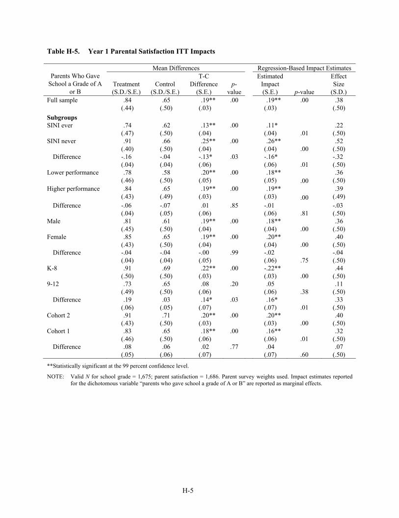
H-5
Table H-5. Year 1 Parental Satisfaction ITT Impacts
Mean Differences Regression-Based Impact Estimates Parents Who Gave
School a Grade of A or B
Treatment (S.D./S.E.)
Control (S.D./S.E.)
T-C Difference
(S.E.) p-
value
Estimated Impact (S.E.) p-value
Effect Size
(S.D.) Full sample .84
(.44) .65
(.50) .19**
(.03) .00
.19**
(.03) .00 .38
(.50) Subgroups SINI ever .74
(.47) .62
(.50) .13**
(.04) .00
.11*
(.04) .01 .22
(.50) SINI never .91
(.40) .66
(.50) .25**
(.04) .00
.26**
(.04) .00 .52
(.50) Difference -.16
(.04) -.04 (.04)
-.13* (.06)
.03
-.16* (.06) .01
-.32 (.50)
Lower performance .78 (.46)
.58 (.50)
.20** (.05)
.00
.18** (.05) .00
.36 (.50)
Higher performance .84 (.43)
.65 (.49)
.19** (.03)
.00
.19** (.03) .00
.39 (.49)
Difference -.06 (.04)
-.07 (.05)
.01 (.06)
.85
-.01 (.06) .81
-.03 (.50)
Male .81 (.45)
.61 (.50)
.19** (.04)
.00
.18** (.04) .00
.36 (.50)
Female .85 (.43)
.65 (.50)
.19** (.04)
.00
.20** (.04) .00
.40 (.50)
Difference -.04 (.04)
-.04 (.04)
-.00 (.05)
.99
-.02 (.06) .75
-.04 (.50)
K-8 .91 (.50)
.69 (.50)
.22** (.03)
.00
-.22** (.03) .00
.44 (.50)
9-12 .73 (.49)
.65 (.50)
.08 (.06)
.20
.05 (.06) .38
.11 (.50)
Difference .19 (.06)
.03 (.05)
.14* (.07)
.03
.16* (.07) .01
.33 (.50)
Cohort 2 .91 (.43)
.71 (.50)
.20** (.03)
.00
.20** (.03) .00
.40 (.50)
Cohort 1 .83 (.46)
.65 (.50)
.18** (.06)
.00
.16** (.06) .01
.32 (.50)
Difference .08 (.05)
.06 (.06)
.02 (.07)
.77
.04 (.07) .60
.07 (.50)
**Statistically significant at the 99 percent confidence level.
NOTE: Valid N for school grade = 1,675; parent satisfaction = 1,686. Parent survey weights used. Impact estimates reported for the dichotomous variable “parents who gave school a grade of A or B” are reported as marginal effects.

H-6
Table H-6. Year 1 Parental Satisfaction ITT Impacts
Mean Differences Regression-Based Impact Estimates Average Grade
Parent Gave School (5.0 Scale)
Treatment (S.D./S.E.)
Control (S.D./S.E.)
T-C Difference
(S.E.) p-
value
Estimated Impact (S.E.) p-value
Effect Size
(S.D.) Full sample 4.02
(1.01) 3.57
(1.11) .45**
(.06) .00
.41**
(.06) .00 .37
(1.11) Subgroups SINI ever 3.84
(1.04) 3.45
(1.16) .39**
(.10) .00
.33**
(.10) .00 .28
(1.16) SINI never 4.16
(.96) 3.65
(1.06) .51**
(.08) .00
.48**
(.08) .00 .45
(1.06) Difference -.32
(.07) -.20
(1.11) -.12 (.13)
.35
-.15 (.13) .23
-.14 (1.11)
Lower performance 3.91 (1.09)
3.37 (1.16)
.54** (.12)
.00
.46** (.12) .00
.40 (1.16)
Higher performance 4.07 (.96)
3.66 (1.07)
.42** (.07)
.00
.39** (.07) .00
.36 (1.07)
Difference -.16* (.07)
-.28* (.12)
.12 (.14)
.37
.07 (.13) .59
.07 (1.11)
Male 3.97 (1.03)
3.53 (1.11)
.44** (.09)
.00
.39** (.09) .00
.35 (1.11)
Female 4.07 (.98)
3.60 (1.11)
.47** (.09)
.00
.44** (.08) .00
.39 (1.11)
Difference -.10 (.07)
-.07 (.10)
-.02 (.12)
.85
-.05 (.12) .68
-.04 (1.11)
K-8 4.08 (1.01)
3.58 (1.12)
.50** (.07)
.00
.47** (.07) .00
.42 (1.12)
9-12 3.76 (.95)
3.51 (1.06)
.24 (.13)
.06
.16 (.13) .21
.15 (1.06)
Difference .32 (.11)
.07 (.11)
.25 (.15)
.09
.30* (.15) .04
.27 (1.11)
Cohort 2 4.06 (1.00)
3.61 (1.10)
.44** (.07)
.00
.41** (.07) .00
.37 (1.10)
Cohort 1 3.88 (1.02)
3.40 (1.12)
.48** (.15)
.00
.42** (.14) .00
.38 (1.12)
Difference .18* (.09)
.21 (.14)
-.03 (.16)
.84
-.01 (.16) .96
-.01 (1.11)
**Statistically significant at the 99 percent confidence level.
NOTE: Valid N for school grade = 1,675; parent satisfaction = 1,686. Parent survey weights used. Impact estimates reported for the dichotomous variable “parents who gave school a grade of A or B” are reported as marginal effects.
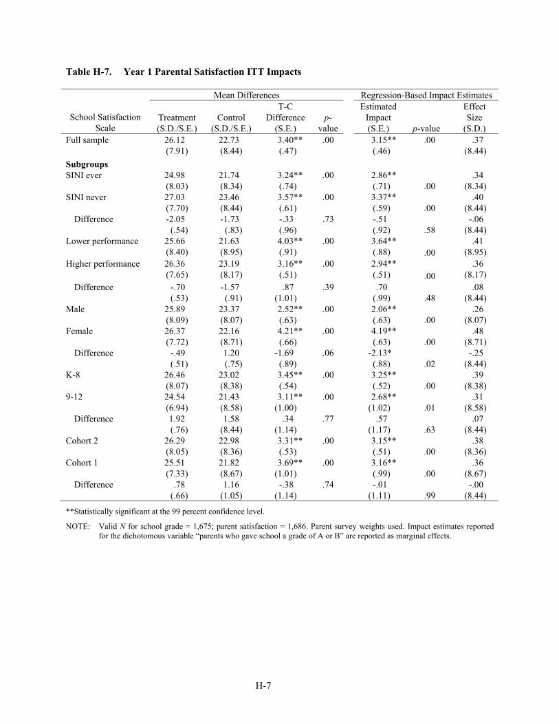
H-7
Table H-7. Year 1 Parental Satisfaction ITT Impacts
Mean Differences Regression-Based Impact Estimates
School Satisfaction Scale
Treatment (S.D./S.E.)
Control (S.D./S.E.)
T-C Difference
(S.E.) p-
value
Estimated Impact (S.E.) p-value
Effect Size
(S.D.) Full sample 26.12
(7.91) 22.73 (8.44)
3.40** (.47)
.00
3.15** (.46)
.00 .37 (8.44)
Subgroups SINI ever 24.98
(8.03) 21.74 (8.34)
3.24** (.74)
.00
2.86** (.71) .00
.34 (8.34)
SINI never 27.03 (7.70)
23.46 (8.44)
3.57** (.61)
.00
3.37** (.59) .00
.40 (8.44)
Difference -2.05 (.54)
-1.73 (.83)
-.33 (.96)
.73
-.51 (.92) .58
-.06 (8.44)
Lower performance 25.66 (8.40)
21.63 (8.95)
4.03** (.91)
.00
3.64** (.88) .00
.41 (8.95)
Higher performance 26.36 (7.65)
23.19 (8.17)
3.16** (.51)
.00
2.94** (.51) .00
.36 (8.17)
Difference -.70 (.53)
-1.57 (.91)
.87 (1.01)
.39
.70 (.99) .48
.08 (8.44)
Male 25.89 (8.09)
23.37 (8.07)
2.52** (.63)
.00
2.06** (.63) .00
.26 (8.07)
Female 26.37 (7.72)
22.16 (8.71)
4.21** (.66)
.00
4.19** (.63) .00
.48 (8.71)
Difference -.49 (.51)
1.20 (.75)
-1.69 (.89)
.06
-2.13* (.88) .02
-.25 (8.44)
K-8 26.46 (8.07)
23.02 (8.38)
3.45** (.54)
.00
3.25** (.52) .00
.39 (8.38)
9-12 24.54 (6.94)
21.43 (8.58)
3.11** (1.00)
.00
2.68** (1.02) .01
.31 (8.58)
Difference 1.92 (.76)
1.58 (8.44)
.34 (1.14)
.77
.57 (1.17) .63
.07 (8.44)
Cohort 2 26.29 (8.05)
22.98 (8.36)
3.31** (.53)
.00
3.15** (.51) .00
.38 (8.36)
Cohort 1 25.51 (7.33)
21.82 (8.67)
3.69** (1.01)
.00
3.16** (.99) .00
.36 (8.67)
Difference .78 (.66)
1.16 (1.05)
-.38 (1.14)
.74
-.01 (1.11) .99
-.00 (8.44)
**Statistically significant at the 99 percent confidence level.
NOTE: Valid N for school grade = 1,675; parent satisfaction = 1,686. Parent survey weights used. Impact estimates reported for the dichotomous variable “parents who gave school a grade of A or B” are reported as marginal effects.
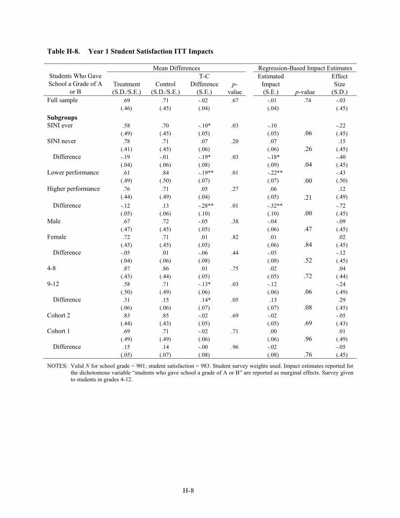
H-8
Table H-8. Year 1 Student Satisfaction ITT Impacts
Mean Differences Regression-Based Impact Estimates Students Who Gave School a Grade of A
or B Treatment (S.D./S.E.)
Control (S.D./S.E.)
T-C Difference
(S.E.) p-
value
Estimated Impact (S.E.) p-value
Effect Size
(S.D.) Full sample .69
(.46) .71
(.45) -.02 (.04)
.67
-.01 (.04)
.74 -.03 (.45)
Subgroups SINI ever .58
(.49) .70
(.45) -.10* (.05)
.03
-.10 (.05) .06
-.22 (.45)
SINI never .78 (.41)
.71 (.45)
.07 (.06)
.20
.07 (.06) .26
.15 (.45)
Difference -.19 (.04)
-.01 (.06)
-.19* (.08)
.03
-.18* (.09) .04
-.40 (.45)
Lower performance .61 (.49)
.84 (.50)
-.19** (.07)
.01
-.22** (.07) .00
-.43 (.50)
Higher performance .76 (.44)
.71 (.49)
.05 (.04)
.27
.06 (.05) .21
.12 (.49)
Difference -.12 (.05)
.13 (.06)
-.28** (.10)
.01
-.32** (.10) .00
-.72 (.45)
Male .67 (.47)
.72 (.45)
-.05 (.05)
.38
-.04 (.06) .47
-.09 (.45)
Female .72 (.45)
.71 (.45)
.01 (.05)
.82
.01 (.06) .84
.02 (.45)
Difference -.05 (.04)
.01 (.06)
-.06 (.08)
.44
-.05 (.08) .52
-.12 (.45)
4-8 .87 (.43)
.86 (.44)
.01 (.05)
.75
.02 (.05) .72
.04 (.44)
9-12 .58 (.50)
.71 (.49)
-.13* (.06)
.03
-.12 (.06) .06
-.24 (.49)
Difference .31 (.06)
.15 (.06)
.14* (.07)
.05
.13 (.07) .08
.29 (.45)
Cohort 2 .83 (.44)
.85 (.43)
-.02 (.05)
.69
-.02 (.05) .69
-.05 (.43)
Cohort 1 .69 (.49)
.71 (.49)
-.02 (.06)
.71
.00 (.06) .96
.01 (.49)
Difference .15 (.05)
.14 (.07)
-.00 (.08)
.96
-.02 (.08) .76
-.05 (.45)
NOTES: Valid N for school grade = 901; student satisfaction = 983. Student survey weights used. Impact estimates reported for the dichotomous variable “students who gave school a grade of A or B” are reported as marginal effects. Survey given to students in grades 4-12.

H-9
Table H-9. Year 1 Student Satisfaction ITT Impacts
Mean Differences Regression-Based Impact Estimates Average Grade
Student Gave School (5.0 Scale)
Treatment (S.D./S.E.)
Control (S.D./S.E.)
T-C Difference
(S.E.) p-
value
Estimated Impact (S.E.) p-value
Effect Size
(S.D.) Full sample 3.98
(1.03) 3.98
(1.00) -.00 (.09)
.99
.00 (.09)
.99 .00 (1.00)
Subgroups SINI ever 3.75
(1.08) 3.85
(1.05) -.10 (.13)
.43
-.08 (.13) .55 -.07
(1.05) SINI never 4.16
(.94) 4.07 (.95)
.09 (.11)
.42
.07 (.12) .57 .07
(.95) Difference -.42
(.10) -.22 (.14)
-.19 (.17)
.27
-.14 (.17) .41 -.14
(1.00) Lower performance 3.82
(1.04) 4.15 (.88)
-.33* (.15)
.03
-.34 (.14) .02 -.38
(.88) Higher performance 4.04
(1.02) 3.92
(1.03) .12
(.10) .25
.13
(.11) .24 .12
(1.03) Difference -.22
(.12) .23
(.15) -.45* (.19)
.02
-.46** (.18) .01 -.46
(1.00) Male 3.92
(1.03) 3.97 (.99)
-.05 (.13)
.67
-.05 (.70) .70 -.05
(.99) Female 4.03
(1.02) 3.98
(1.01) .04
(.12) .72
.05
(.12) .70 .05 (1.01)
Difference -.11 (.10)
-.01 (.14)
-.10 (.18)
.58
-.09 (.17) .58 -.09
(1.00) 4-8 4.11
(.98) 4.08 (.97)
.03 (.10)
.75
.04 (.10) .71 .04
(.97) 9-12 3.38
(1.00) 3.56
(1.01) -.18 (.15)
.22
-.16 (.15) .30 -.16
(1.01) Difference .73
(.13) .52
(.13) .22
(.18) .22
.20
(.18) .27 .20 (1.00)
Cohort 2 4.06 (1.00)
4.11 (.93)
-.05 (.10)
.63
-.05 (.10) .61 -.06
(.93) Cohort 1 3.68
(1.05) 3.57
(1.10) .11
(.16) .50
.18
(.15) .23 .17 (1.10)
Difference .38 (.11)
.53 (.15)
-.16 (.19)
.41
-.24 (.18) .19 -.24
(1.00)
NOTES: Valid N for school grade = 901; student satisfaction = 983. Student survey weights used. Impact estimates reported for the dichotomous variable “students who gave school a grade of A or B” are reported as marginal effects. Survey given to students in grades 4-12.
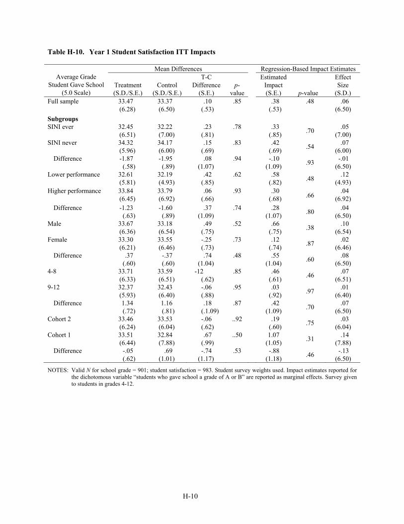
H-10
Table H-10. Year 1 Student Satisfaction ITT Impacts
Mean Differences Regression-Based Impact Estimates Average Grade
Student Gave School (5.0 Scale)
Treatment (S.D./S.E.)
Control (S.D./S.E.)
T-C Difference
(S.E.) p-
value
Estimated Impact (S.E.) p-value
Effect Size
(S.D.) Full sample 33.47
(6.28) 33.37 (6.50)
.10 (.53)
.85
.38 (.53)
.48 .06 (6.50)
Subgroups SINI ever 32.45
(6.51) 32.22 (7.00)
.23 (.81)
.78
.33 (.85) .70 .05
(7.00) SINI never 34.32
(5.96) 34.17 (6.00)
.15 (.69)
.83
.42 (.69) .54 .07
(6.00) Difference -1.87
(.58) -1.95 (.89)
.08 (1.07)
.94
-.10 (1.09) .93 -.01
(6.50) Lower performance 32.61
(5.81) 32.19 (4.93)
.42 (.85)
.62
.58 (.82) .48 .12
(4.93) Higher performance 33.84
(6.45) 33.79 (6.92)
.06 (.66)
.93
.30 (.68) .66
.04 (6.92)
Difference -1.23 (.63)
-1.60 (.89)
.37 (1.09)
.74
.28 (1.07) .80 .04
(6.50) Male 33.67
(6.36) 33.18 (6.54)
.49 (.75)
.52
.66 (.75) .38 .10
(6.54) Female 33.30
(6.21) 33.55 (6.46)
-.25 (.73)
.73
.12 (.74) .87 .02
(6.46) Difference .37
(.60) -.37 (.60)
.74 (1.04)
.48
.55 (1.04) .60 .08
(6.50) 4-8 33.71
(6.33) 33.59 (6.51)
-12 (.62)
.85
.46 (.61) .46 .07
(6.51) 9-12 32.37
(5.93) 32.43 (6.40)
-.06 (.88)
.95
.03 (.92) .97 .01
(6.40) Difference 1.34
(.72) 1.16 (.81)
.18 (.1.09)
.87
.42 (1.09) .70 .07
(6.50) Cohort 2 33.46
(6.24) 33.53 (6.04)
-.06 (.62)
..92
.19 (.60) .75 .03
(6.04) Cohort 1 33.51
(6.44) 32.84 (7.88)
.67 (.99)
..50
1.07 (1.05) .31 .14
(7.88) Difference -.05
(.62) .69
(1.01) -.74
(1.17) .53
-.88
(1.18) .46 -.13 (6.50)
NOTES: Valid N for school grade = 901; student satisfaction = 983. Student survey weights used. Impact estimates reported for the dichotomous variable “students who gave school a grade of A or B” are reported as marginal effects. Survey given to students in grades 4-12.
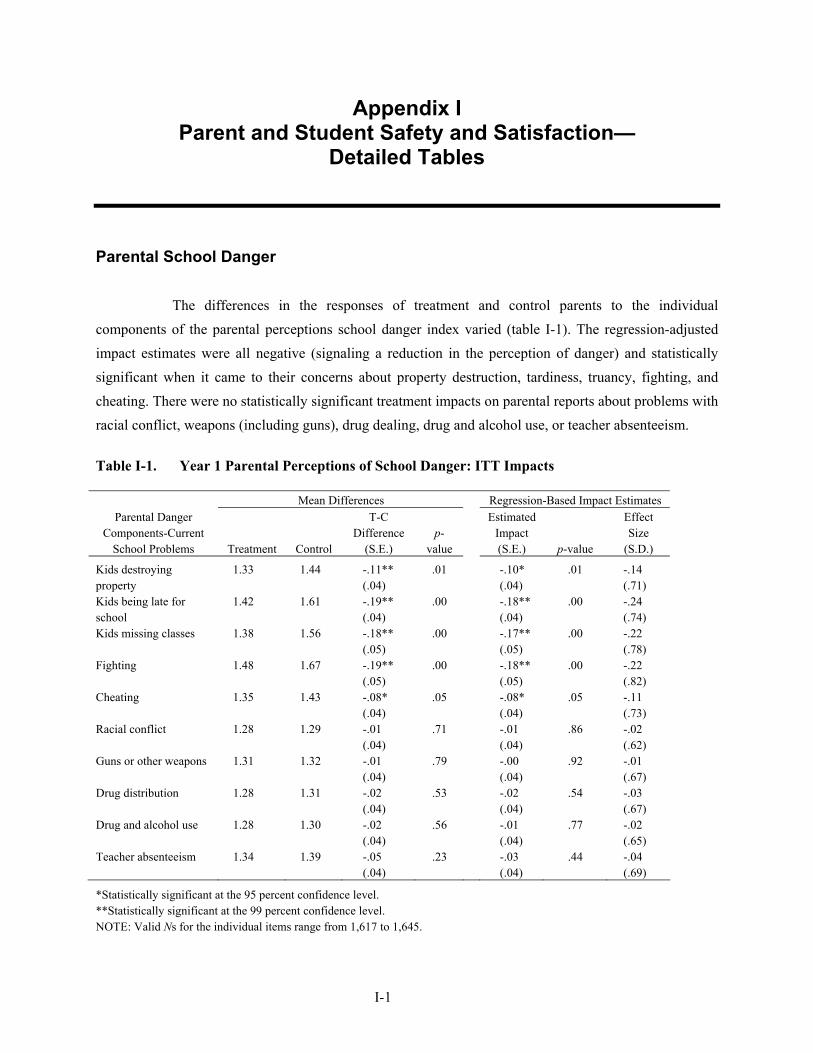
I-1
Appendix I Parent and Student Safety and Satisfaction—
Detailed Tables
Parental School Danger
The differences in the responses of treatment and control parents to the individual components of the parental perceptions school danger index varied (table I-1). The regression-adjusted impact estimates were all negative (signaling a reduction in the perception of danger) and statistically significant when it came to their concerns about property destruction, tardiness, truancy, fighting, and cheating. There were no statistically significant treatment impacts on parental reports about problems with racial conflict, weapons (including guns), drug dealing, drug and alcohol use, or teacher absenteeism.
Table I-1. Year 1 Parental Perceptions of School Danger: ITT Impacts
Mean Differences Regression-Based Impact Estimates Parental Danger
Components-Current School Problems Treatment Control
T-C Difference
(S.E.) p-
value
Estimated Impact (S.E.) p-value
Effect Size
(S.D.)
Kids destroying property
1.33 1.44 -.11** (.04)
.01 -.10* (.04)
.01 -.14 (.71)
Kids being late for school
1.42 1.61 -.19** (.04)
.00 -.18** (.04)
.00 -.24 (.74)
Kids missing classes 1.38 1.56 -.18** (.05)
.00 -.17** (.05)
.00 -.22 (.78)
Fighting 1.48 1.67 -.19** (.05)
.00 -.18** (.05)
.00 -.22 (.82)
Cheating 1.35 1.43 -.08* (.04)
.05 -.08* (.04)
.05 -.11 (.73)
Racial conflict 1.28 1.29 -.01 (.04)
.71 -.01 (.04)
.86 -.02 (.62)
Guns or other weapons 1.31 1.32 -.01 (.04)
.79 -.00 (.04)
.92 -.01 (.67)
Drug distribution 1.28 1.31 -.02 (.04)
.53 -.02 (.04)
.54 -.03 (.67)
Drug and alcohol use 1.28 1.30 -.02 (.04)
.56 -.01 (.04)
.77 -.02 (.65)
Teacher absenteeism 1.34 1.39 -.05 (.04)
.23 -.03 (.04)
.44 -.04 (.69)
*Statistically significant at the 95 percent confidence level. **Statistically significant at the 99 percent confidence level. NOTE: Valid Ns for the individual items range from 1,617 to 1,645.
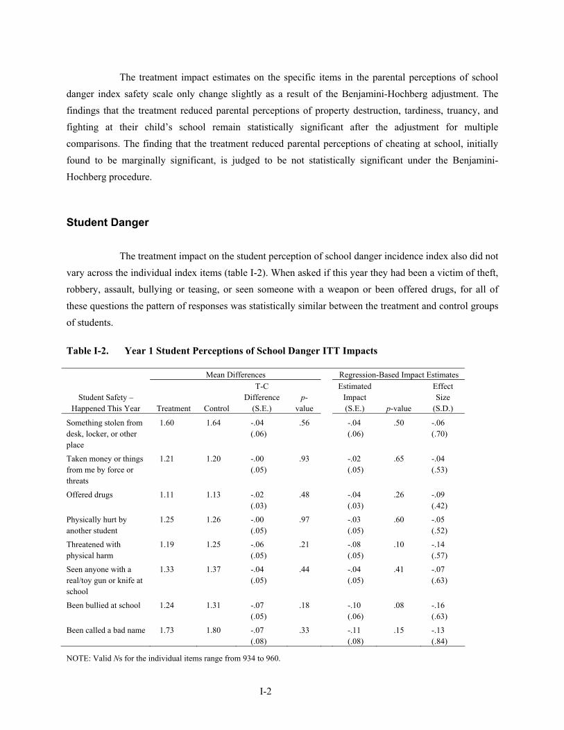
I-2
The treatment impact estimates on the specific items in the parental perceptions of school danger index safety scale only change slightly as a result of the Benjamini-Hochberg adjustment. The findings that the treatment reduced parental perceptions of property destruction, tardiness, truancy, and fighting at their child’s school remain statistically significant after the adjustment for multiple comparisons. The finding that the treatment reduced parental perceptions of cheating at school, initially found to be marginally significant, is judged to be not statistically significant under the Benjamini-Hochberg procedure.
Student Danger
The treatment impact on the student perception of school danger incidence index also did not vary across the individual index items (table I-2). When asked if this year they had been a victim of theft, robbery, assault, bullying or teasing, or seen someone with a weapon or been offered drugs, for all of these questions the pattern of responses was statistically similar between the treatment and control groups of students.
Table I-2. Year 1 Student Perceptions of School Danger ITT Impacts
Mean Differences Regression-Based Impact Estimates
Student Safety – Happened This Year Treatment Control
T-C Difference
(S.E.) p-
value
Estimated Impact (S.E.) p-value
Effect Size
(S.D.)
Something stolen from desk, locker, or other place
1.60 1.64 -.04 (.06)
.56 -.04 (.06)
.50 -.06 (.70)
Taken money or things from me by force or threats
1.21 1.20 -.00 (.05)
.93 -.02 (.05)
.65 -.04 (.53)
Offered drugs 1.11 1.13 -.02 (.03)
.48 -.04 (.03)
.26 -.09 (.42)
Physically hurt by another student
1.25 1.26 -.00 (.05)
.97 -.03 (.05)
.60 -.05 (.52)
Threatened with physical harm
1.19 1.25 -.06 (.05)
.21 -.08 (.05)
.10 -.14 (.57)
Seen anyone with a real/toy gun or knife at school
1.33 1.37 -.04 (.05)
.44 -.04 (.05)
.41 -.07 (.63)
Been bullied at school 1.24 1.31 -.07 (.05)
.18 -.10 (.06)
.08 -.16 (.63)
Been called a bad name 1.73 1.80 -.07 (.08)
.33 -.11 (.08)
.15 -.13 (.84)
NOTE: Valid Ns for the individual items range from 934 to 960.

I-3
Parental Satisfaction
The impact of the Program on parental satisfaction is almost entirely consistent across the 12 individual components of the satisfaction scale, including class size, facilities, academic quality, safety, discipline, and the racial mix of students (table I-3). The parents of students offered a scholarship were significantly more satisfied than the parents of control group students with every surveyed aspect of their child’s school, with the exception of the regression-based estimate of the Program’s impact on satisfaction with “Services for Students with Special Needs” which was positive but not statistically significant.
Table I-3. Year 1 Parental Satisfaction ITT Impacts
Mean Differences Regression-Based Impact Estimates
Student Safety Treatment Control
T-C Difference
(S.E.) p-
value
Estimated Impact (S.E.) p-value
Effect Size
(S.D.)
Location 3.27 3.09 .18** (.05)
.00 .16** (.05)
.00 .19 (.85)
Safety 3.24 2.93 .31** (.05)
.00 .29** (.05)
.00 .32 (.91)
Class sizes 3.21 2.81 .40** (.05)
.00 .39** (.05)
.00 .42 (.93)
School facilities 3.13 2.80 .33** (.05)
.00 .32** (.05)
.00 .36 (.90)
Respect between teachers and students
3.23 2.98 .25** (.05)
.00 .23** (.05)
.00 .25 (.90)
Teachers inform parents of students’ progress
3.28 2.98 .30** (.05)
.00 .27** (.05)
.00 .29 (.95)
Amount students can observe religious traditions
3.30 2.91 .39** (.07)
.00 .37** (.06)
.00 .31 (1.18)
Parental support for the school
3.18 2.93 .26** (.05)
.00 .23** (.05)
.00 .27 (.85)
Discipline 3.18 2.86 .32** (.05)
.00 .29** (.05)
.00 .31 (.93)
Academic quality 3.21 2.85 .36** (.06)
.00 .33** (.05)
.00 .35 (.95)
Racial mix of students 3.15 2.89 .25** (.05)
.00 .25** (.05)
.00 .28 (.90)
Services for students with special needs
3.70 3.54 .17* (.08)
.04 .14 (.08)
.08 .11 (1.33)
*Statistically significant at the 95 percent confidence level. **Statistically significant at the 99 percent confidence level. NOTE: Valid Ns for the individual items range from 1,589 to 1,659.
I-4
These positive treatment impacts on the individual elements of parental satisfaction with their child’s school were so consistent in the data that the Benjamini-Hochberg adjustment for multiple comparisons did not change the statistical significance of any of them.
Student Satisfaction
There were few differences in how students in the treatment and control groups responded to the individual components of the satisfaction index, with two exceptions (table I-4):
• Treatment students were more likely than control students to say that “there is a lot of
learning at this school;” and
• Treatment students were more likely than control students to say that rules of behavior are strict in their schools.
The two item-specific treatment impacts on student satisfaction were the product of 17 multiple comparisons. They were no longer statistically significant after the application of the Benjamini-Hochberg adjustment; that is, we cannot rule out “false discoveries” as the source of these two seemingly significant treatment impacts on student satisfaction. The general conclusion to be drawn from the evidence on student satisfaction in Year 1 of the OSP experimental evaluation is that the treatment students are no more or less satisfied with their schools than the control students.
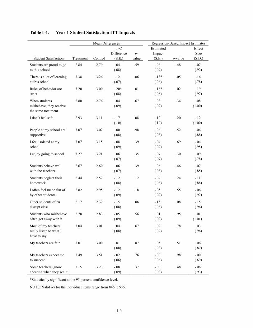
I-5
Table I-4. Year 1 Student Satisfaction ITT Impacts
Mean Differences Regression-Based Impact Estimates
Student Satisfaction Treatment Control
T-C Difference
(S.E.) p-
value
Estimated Impact (S.E.) p-value
Effect Size
(S.D.)
Students are proud to go to this school
2.84 2.79 .04 (.08)
.59 .06 (.09)
.48 .07 (.92)
There is a lot of learning at this school
3.38 3.26 .12 (.07)
.06 .13* (.06)
.05 .16 (.78)
Rules of behavior are strict
3.20 3.00 .20* (.08)
.01 .18* (.08)
.02 .19 (.97)
When students misbehave, they receive the same treatment
2.80 2.76 .04 (.09)
.67 .08 (.09)
.34 .08 (1.00)
I don’t feel safe 2.93 3.11 -.17 (.10)
.08 -.12 (.10)
.20 -.12 (1.00)
People at my school are supportive
3.07 3.07 .00 (.08)
.98 .06 (.08)
.52 .06 (.88)
I feel isolated at my school
3.07 3.15 -.08 (.09)
.39 -.04 (.09)
.69 -.04 (.95)
I enjoy going to school 3.27 3.21 .06 (.07)
.35 .07 (.07)
.30 .09 (.78)
Students behave well with the teachers
2.67 2.60 .06 (.07)
.39 .06 (.08)
.46 .07 (.85)
Students neglect their homework
2.44 2.57 -.12 (.08)
.12 -.09 (.08)
.24 -.11 (.88)
I often feel made fun of by other students
2.82 2.95 -.12 (.09)
.18 -.05 (.09)
.55 -.06 (.97)
Other students often disrupt class
2.17 2.32 -.15 (.08)
.06 -.15 (.08)
.08 -.15 (.96)
Students who misbehave often get away with it
2.78 2.83 -.05 (.09)
.56 .01 (.09)
.95 .01 (1.01)
Most of my teachers really listen to what I have to say
3.04 3.01 .04 (.08)
.67 .02 (.09)
.78 .03 (.96)
My teachers are fair 3.01 3.00 .01 (.08)
.87 .05 (.08)
.51 .06 (.87)
My teachers expect me to succeed
3.49 3.51 -.02 (.06)
.76 -.00 (.06)
.98 -.00 (.69)
Some teachers ignore cheating when they see it
3.15 3.23 -.08 (.09)
.37 -.06 (.08)
.48 -.06 (.93)
*Statistically significant at the 95 percent confidence level.
NOTE: Valid Ns for the individual items range from 846 to 955.
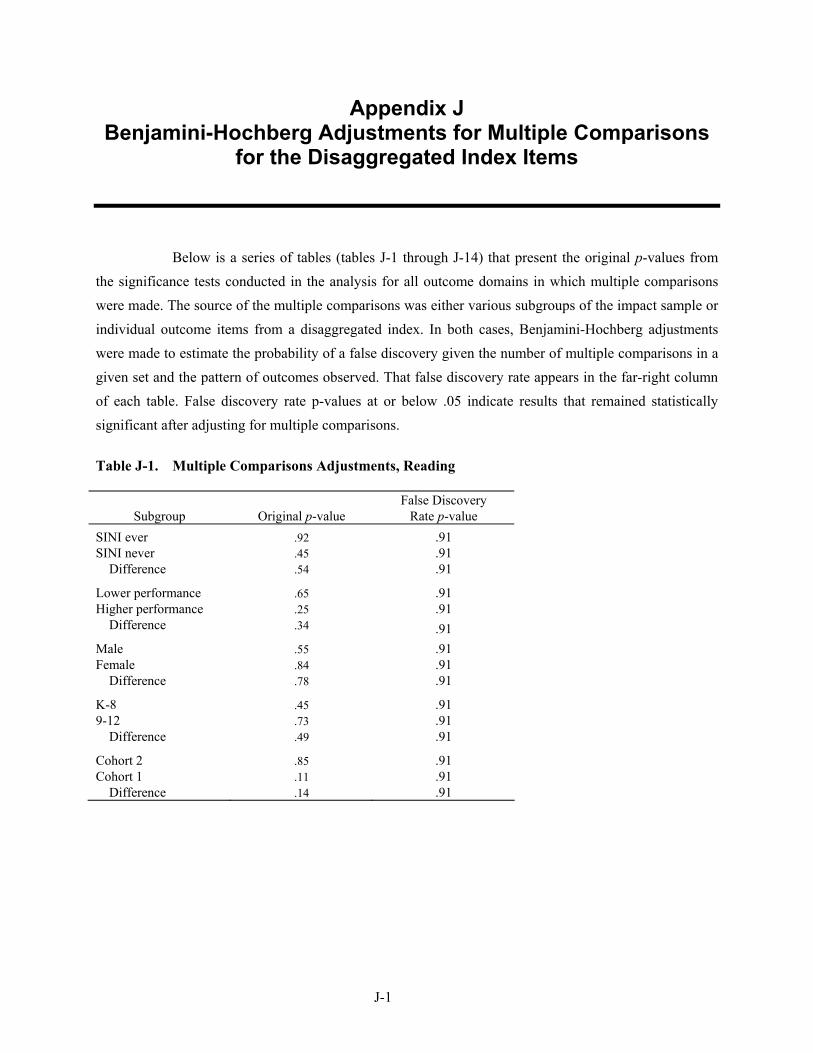
J-1
Appendix J Benjamini-Hochberg Adjustments for Multiple Comparisons
for the Disaggregated Index Items
Below is a series of tables (tables J-1 through J-14) that present the original p-values from the significance tests conducted in the analysis for all outcome domains in which multiple comparisons were made. The source of the multiple comparisons was either various subgroups of the impact sample or individual outcome items from a disaggregated index. In both cases, Benjamini-Hochberg adjustments were made to estimate the probability of a false discovery given the number of multiple comparisons in a given set and the pattern of outcomes observed. That false discovery rate appears in the far-right column of each table. False discovery rate p-values at or below .05 indicate results that remained statistically significant after adjusting for multiple comparisons.
Table J-1. Multiple Comparisons Adjustments, Reading
Subgroup Original p-value False Discovery
Rate p-value SINI ever .92 .91 SINI never .45 .91
Difference .54 .91
Lower performance .65 .91 Higher performance .25 .91
Difference .34 .91 Male .55 .91 Female .84 .91
Difference .78 .91
K-8 .45 .91 9-12 .73 .91
Difference .49 .91
Cohort 2 .85 .91 Cohort 1 .11 .91
Difference .14 .91
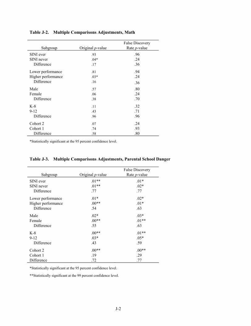
J-2
Table J-2. Multiple Comparisons Adjustments, Math
Subgroup Original p-value False Discovery
Rate p-value SINI ever .93 .96 SINI never .04* .24
Difference .17 .36
Lower performance .81 .94 Higher performance .03* .24
Difference .16 .36 Male .57 .80 Female .06 .24
Difference .38 .70
K-8 .11 .32 9-12 .43 .71
Difference .96 .96
Cohort 2 .07 .24 Cohort 1 .74 .93
Difference .58 .80
*Statistically significant at the 95 percent confidence level.
Table J-3. Multiple Comparisons Adjustments, Parental School Danger
Subgroup Original p-value False Discovery
Rate p-value SINI ever .01** .01* SINI never .01** .02*
Difference .77 .77
Lower performance .01* .02* Higher performance .00** .01*
Difference .54 .63
Male .02* .03* Female .00** .01**
Difference .55 .63
K-8 .00** .01** 9-12 .03* .05*
Difference .43 .59
Cohort 2 .00** .00** Cohort 1 .19 .29 Difference .72 .77
*Statistically significant at the 95 percent confidence level.
**Statistically significant at the 99 percent confidence level.
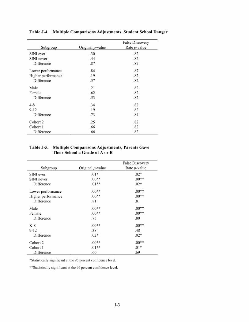
J-3
Table J-4. Multiple Comparisons Adjustments, Student School Danger
Subgroup Original p-value False Discovery
Rate p-value SINI ever .30 .82 SINI never .44 .82
Difference .87 .87
Lower performance .84 .87 Higher performance .19 .82
Difference .57 .82
Male .21 .82 Female .62 .82
Difference .53 .82
4-8 .34 .82 9-12 .19 .82
Difference .73 .84
Cohort 2 .25 .82 Cohort 1 .66 .82
Difference .66 .82 Table J-5. Multiple Comparisons Adjustments, Parents Gave
Their School a Grade of A or B
Subgroup Original p-value False Discovery
Rate p-value SINI ever .01* .02* SINI never .00** .00**
Difference .01** .02*
Lower performance .00** .00** Higher performance .00** .00**
Difference .81 .81
Male .00** .00** Female .00** .00**
Difference .75 .80
K-8 .00** .00** 9-12 .38 .48
Difference .02* .02*
Cohort 2 .00** .00** Cohort 1 .01** .01*
Difference .60 .69
*Statistically significant at the 95 percent confidence level.
**Statistically significant at the 99 percent confidence level.
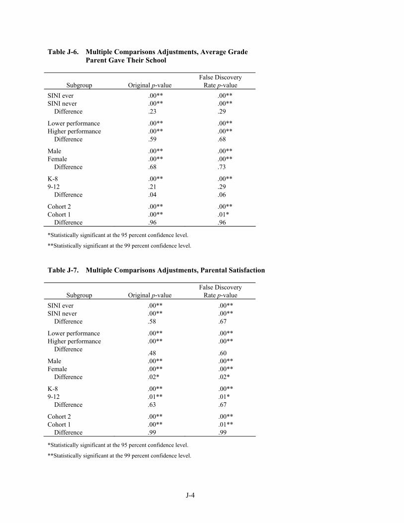
J-4
Table J-6. Multiple Comparisons Adjustments, Average Grade Parent Gave Their School
Subgroup Original p-value False Discovery
Rate p-value SINI ever .00** .00** SINI never .00** .00**
Difference .23 .29
Lower performance .00** .00** Higher performance .00** .00**
Difference .59 .68
Male .00** .00** Female .00** .00**
Difference .68 .73
K-8 .00** .00** 9-12 .21 .29
Difference .04 .06
Cohort 2 .00** .00** Cohort 1 .00** .01*
Difference .96 .96
*Statistically significant at the 95 percent confidence level.
**Statistically significant at the 99 percent confidence level. Table J-7. Multiple Comparisons Adjustments, Parental Satisfaction
Subgroup Original p-value False Discovery
Rate p-value SINI ever .00** .00** SINI never .00** .00**
Difference .58 .67
Lower performance .00** .00** Higher performance .00** .00**
Difference .48 .60 Male .00** .00** Female .00** .00**
Difference .02* .02*
K-8 .00** .00** 9-12 .01** .01*
Difference .63 .67
Cohort 2 .00** .00** Cohort 1 .00** .01**
Difference .99 .99
*Statistically significant at the 95 percent confidence level.
**Statistically significant at the 99 percent confidence level.
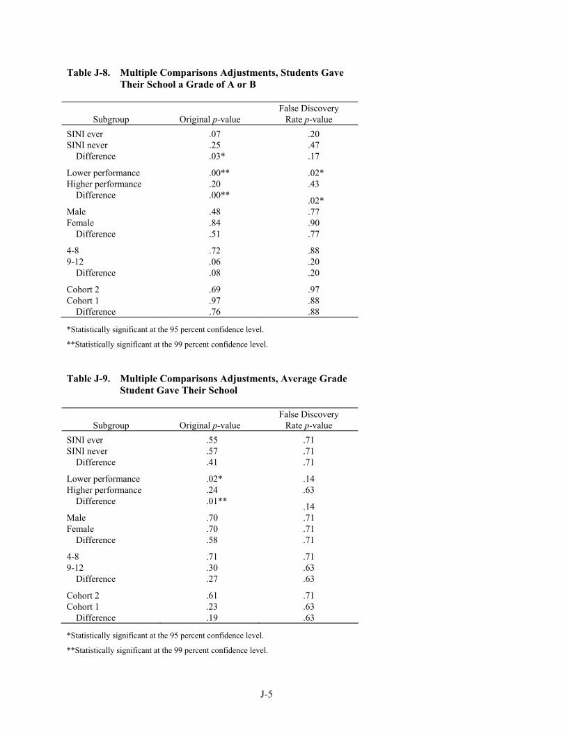
J-5
Table J-8. Multiple Comparisons Adjustments, Students Gave Their School a Grade of A or B
Subgroup Original p-value False Discovery
Rate p-value SINI ever .07 .20 SINI never .25 .47
Difference .03* .17
Lower performance .00** .02* Higher performance .20 .43
Difference .00** .02* Male .48 .77 Female .84 .90
Difference .51 .77
4-8 .72 .88 9-12 .06 .20
Difference .08 .20
Cohort 2 .69 .97 Cohort 1 .97 .88
Difference .76 .88
*Statistically significant at the 95 percent confidence level.
**Statistically significant at the 99 percent confidence level. Table J-9. Multiple Comparisons Adjustments, Average Grade
Student Gave Their School
Subgroup Original p-value False Discovery
Rate p-value SINI ever .55 .71 SINI never .57 .71
Difference .41 .71
Lower performance .02* .14 Higher performance .24 .63
Difference .01** .14 Male .70 .71 Female .70 .71
Difference .58 .71
4-8 .71 .71 9-12 .30 .63
Difference .27 .63
Cohort 2 .61 .71 Cohort 1 .23 .63
Difference .19 .63
*Statistically significant at the 95 percent confidence level.
**Statistically significant at the 99 percent confidence level.

J-6
Table J-10. Multiple Comparisons Adjustments, Student Satisfaction Scale
Subgroup Original p-value False Discovery
Rate p-value SINI ever .70 .97 SINI never .54 .97
Difference .93 .97
Lower performance .48 .97 Higher performance .66 .97
Difference .80 .97 Male .38 .97 Female .87 .97
Difference .60 .97
4-8 .46 .97 9-12 .97 .97
Difference .70 .97
Cohort 2 .75 .97 Cohort 1 .37 .97
Difference .46 .97 Table J-11. Multiple Comparisons Adjustments, Parent School
Danger Items
Subgroup Original p-value False Discovery
Rate p-value Kids destroying property .01* .03* Kids being late for school .00** .00** Kids missing classes .00** .00** Fighting .00** .00** Cheating .05* .10 Racial conflict .86 .92 Guns or other weapons .92 .92 Drug distribution .54 .78 Drug and alcohol use .77 .92 Teacher absenteeism .44 .73
*Statistically significant at the 95 percent confidence level.
**Statistically significant at the 99 percent confidence level.
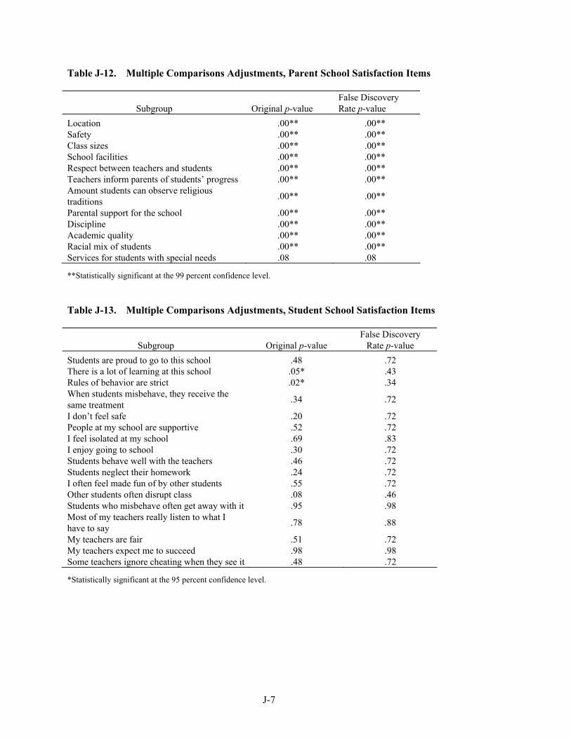
J-7
Table J-12. Multiple Comparisons Adjustments, Parent School Satisfaction Items
Subgroup Original p-value False Discovery Rate p-value
Location .00** .00** Safety .00** .00** Class sizes .00** .00** School facilities .00** .00** Respect between teachers and students .00** .00** Teachers inform parents of students’ progress .00** .00** Amount students can observe religious traditions .00** .00**
Parental support for the school .00** .00** Discipline .00** .00** Academic quality .00** .00** Racial mix of students .00** .00** Services for students with special needs .08 .08
**Statistically significant at the 99 percent confidence level. Table J-13. Multiple Comparisons Adjustments, Student School Satisfaction Items
Subgroup Original p-value False Discovery
Rate p-value Students are proud to go to this school .48 .72 There is a lot of learning at this school .05* .43 Rules of behavior are strict .02* .34 When students misbehave, they receive the same treatment .34 .72
I don’t feel safe .20 .72 People at my school are supportive .52 .72 I feel isolated at my school .69 .83 I enjoy going to school .30 .72 Students behave well with the teachers .46 .72 Students neglect their homework .24 .72 I often feel made fun of by other students .55 .72 Other students often disrupt class .08 .46 Students who misbehave often get away with it .95 .98 Most of my teachers really listen to what I have to say .78 .88
My teachers are fair .51 .72 My teachers expect me to succeed .98 .98 Some teachers ignore cheating when they see it .48 .72
*Statistically significant at the 95 percent confidence level.
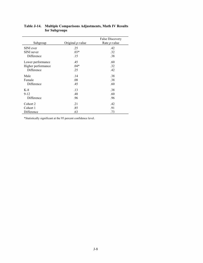
J-8
Table J-14. Multiple Comparisons Adjustments, Math IV Results for Subgroups
Subgroup Original p-value False Discovery
Rate p-value SINI ever .25 .42 SINI never .03* .32
Difference .15 .38
Lower performance .45 .60 Higher performance .04* .32
Difference .25 .42
Male .14 .38 Female .08 .38
Difference .45 .60
K-8 .13 .38 9-12 .48 .60
Difference .96 .96
Cohort 2 .21 .42 Cohort 1 .85 .91 Difference .63 .73
*Statistically significant at the 95 percent confidence level.