evaluation of the partition function of fermions using ... · evaluation of the partition function...
TRANSCRIPT

%%%
¡¡
¡
,,
,,
´´
©©e
ee@
@@l
ll
QQQ
HHPPP XXX hhhh (((( ³³© IFTInstituto de Fısica Teorica
Universidade Estadual Paulista
DISSERTACAO DE MESTRADO IFT–D.013/09
Evaluation of the partition function of fermions using Grassmann
coherent states without path integrals
Daniel Fernando Reyes Castillo
Orientador
Gastao Inacio Krein
Outubro de 2009

Agradecimentos
I want to take the opportunity to thank many people:
First, I want to thank my parents for all the support they gave me through all my
life, even with that little fear of not knowing what my life was going to be. Probably
they believed in me more than they should have.
To my family and friends as a whole for standing such a smartass as myself. And
for helping me understand (voluntarily but most of the time involuntarily) the im-
portance of a more complete development as a human being.
To my advisor, for the patience he had (and still has) to understand my not even
portunhol, and for all the discussions we had that cleared up a lot of doubts I had.
And for solidifying in me the idea of the necessity (not only the importance) of
challenging established ideas.
To all the friends I made here that became my family, because these experiences
without them would be just an academic experience and not an humanistic one as
well.
And at last, but not the least important, to CAPES for the financial help, that
allowed me to study without any preoccupation.
i

Resumo
A presente dissertacao tem como objetivo principal fazer uma revisao sobre o
uso de estados coerentes para calcular a funcao de particao gran canonica de sis-
temas fermionicos, sem empregar integrais de trajetoria. Apos discutir um metodo
de calculo baseado numa expansao de altas temperaturas, formulamos uma teo-
ria de perturbacao otimizada empregando campos auxiliares via transformacao de
Hubbard-Stratonovich. Aproximacoes nao perturbativas tradicionais de campo me-
dio tipo Hartree-Fock e de BCS sao obtidas em ordem zero da teoria de pertubacao
otimizada. Correcoes nao perturbativas a aproximacao de ordem zero sao imple-
mentadas usando uma expansao em potencias de uma interacao modificada, em que
os efeitos dos campos medios sao subtraıdos da interacao original do Hamiltoniano
da teoria.
Palavras Chaves: Estados coerentes, Integrais de trajetoria, Fermions, Algebra
de Grassmann, Transformacao de Hubbard-Stratonovich, Teoria de perturbacao
otimizada
Areas do conhecimento: Fısica Nuclear, Teoria de Campos e Partıculas Ele-
mentares, Fısica da Materia Condensada
ii
Abstract
The primary aim of the dissertation is to review the use of coherent states for
the calculation of the grand canonical partition function for fermion systems, with-
out employing path integrals. After discussing a calculational method based on a
high temperature expansion, we formulate an optimized perturbation theory em-
ploying external fields via the Hubbard-Stratonovich transformation. Traditional
non-perturbative mean field approximations like Hartree-Fock and BCS are obtained
in zeroth order in the optimized perturbation theory. Non-perturbative corrections
to the zeroth order approximation are implemented through a power series expan-
sion of a modified interaction,where the effects of the mean fields are subtracted
from the original interaction of the Hamiltonian of the theory.
iii
Indice
1 Introduction 1
2 Second Quantization Formalism 6
2.1 Many-particle bases . . . . . . . . . . . . . . . . . . . . . . . . . . . . 6
2.2 Many-body operators . . . . . . . . . . . . . . . . . . . . . . . . . . . 10
2.3 Creation and annihilation operators . . . . . . . . . . . . . . . . . . . 12
2.4 Fock space . . . . . . . . . . . . . . . . . . . . . . . . . . . . . . . . . 14
2.5 Change of representation . . . . . . . . . . . . . . . . . . . . . . . . . 15
3 Coherent states and Path Integrals at Finite Temperature 19
3.1 Feynman path integral in quantum mechanics . . . . . . . . . . . . . 20
3.2 Coherent states for bosons . . . . . . . . . . . . . . . . . . . . . . . . 22
3.3 Grassmann algebras . . . . . . . . . . . . . . . . . . . . . . . . . . . . 28
3.4 Coherent states for fermions . . . . . . . . . . . . . . . . . . . . . . . 31
3.5 Path integral for bosons and fermions . . . . . . . . . . . . . . . . . . 36
4 The Niteroi Method 42
4.1 Coherent-state representation of the trace of (Ω)s . . . . . . . . . . . 42
4.2 Explicit expression for Ω¯(ξ∗, ξ) . . . . . . . . . . . . . . . . . . . . . 44
4.3 Evaluation of the Grassmann integrals in Tr(Ω)s . . . . . . . . . . . . 45
5 Applications to simple problems and possible extensions 49
5.1 Non-interacting non-relativistic Fermi gas . . . . . . . . . . . . . . . . 49
5.2 Interacting nonrelativistic Fermions, canonical transformations . . . . 53
5.3 Perturbation on the mean field . . . . . . . . . . . . . . . . . . . . . . 56
5.4 Optimized perturbation theory . . . . . . . . . . . . . . . . . . . . . 59
6 Conclusions and perspectives 64
A Two-body operators - Change of representation 67
iv

B Evaluation of U(rn+1, ε; rn, 0) 69
C Closure for bosonic coherent states 71
D Numerical values of the fundamental Grassmann integrals 73
E Symmetrical term for the exponential in the partition function 77
F The Feynman ordering label technique 79
Referencias 84
v

Capıtulo 1
Introduction
The present dissertation is primarily a review on the use of coherent states in the
evaluation of the quantum grand canonical partition function of a many-particle
system at finite temperature. The main focus of the dissertation are systems of
spin-1/2 fermions. The grand canonical partition function is the fundamental quan-
tity in the mathematical treatment of many-body systems from which all physical
quantities can be derived [1, 2]. However, it can scarcely be calculated in closed
form, a fact that is not surprising in view of the intractability of the many-body
problem. On the other hand, there is great activity on the development of efficient
numerical methods for calculating the partition function non-perturbatively. Monte
Carlo methods have been central to such methods, in particular in the context of
quantum field theory problems. The basic strategy of the Monte Carlo (MC) [3]
method in field theory is to express the trace over field configurations in terms
of a path integral so that the problem is reduced to the evaluation of a multidi-
mensional integral using importance sampling [4]. Path integral formulations of
fermion quantum fields involve the use of anti-commuting Grassmann variables [5],
providing a very useful tool for implementing covariant perturbation theory calcu-
lations in gauge theories [6] and super-symmetric field theories [7]. However, this
approach is problematic for nonperturbative approaches like the MC method. For
models (or theories) involving boson-fermion couplings, like Quantum Electrody-
namics (QED) and Quantum Chromodynamics (QCD), invariably the application
of the MC method involves a formal, exact integration over the Grassmann vari-
ables in favor of determinants that depend only on the boson fields. For models
involving only fermion fields the application of the MC method involves the use of a
Hubbard-Stratonovich transformation [8]. This method introduces auxiliary boson
fields so that the self-interacting part of the interaction becomes quadratic so that
the Grassmann variables representing fermion fields can be integrated. Again this
leads to determinants that involve only boson fields. In many cases the resulting
1

determinants can be rewritten as path integrals over additional boson fields and the
problem is then reduced to the evaluation of multidimensional integrals over boson
degrees of freedom. The problem with this approach is that the resulting determi-
nants are in general complex (when not complex, they might not be positive) and the
use of a MC approach becomes very inefficient or even inapplicable. This problem
of a non-positive determinant is known in the literature as the sign problem.
An alternative to the path integral formulation of the grand canonical parti-
tion function is the direct evaluation of the trace over Grassmann variables. A
particularly interesting novel approach in this direction was introduced a few years
ago by Thomaz and collaborators [9]. The method is based on the high temper-
ature expansion of the Boltzmann factor in the partition function and makes use
of the coherent-state representation of the trace [1]. Each term of the expansion is
evaluated exactly exploiting the anti-commuting nature of the Grassmann numbers.
This novel method builds on previous experience in calculating the high-temperature
expansion of the partition function of an anharmonic fermionic oscillator on a lat-
tice [10] and of the one-dimensional Hubbard model [11]. Crucial to the method
are two results obtained by Thomaz and collaborators in two separate publications.
First, Charret, de Souza and Thomaz [12] have shown that the moments of a Gaus-
sian Grassmann multi-variable integral are related to the co-factors of the matrix
of the Gaussian exponential. This result is important because the expansion of the
Boltzmann factor requires the evaluation of a trace of multiple products of operators.
The trace of a product of operators can be expressed in terms of matrix elements in a
coherent-state representation and this leads to a multi-variable integral over Grass-
mann numbers. Second, I.C. Charret, Correa Silva, S.M. de Souza, O. Rojas Santos,
and M.T. Thomaz [13] have shown that the matrix related to the co-factors men-
tioned above can be diagonalized analytically through a similarity transformation.
This result is valid for any dimensionality of the matrix and is model independent,
in that it depends only on the kinematical aspects of the approach. This was a
tremendous achievement, since despite the closed form of the result of the multidi-
mensional Grassmann integral in terms of co-factors, their explicit evaluation is still
a formidable task.
In the present dissertation we review this approach developed by Thomaz and
collaborators. We name this approach the Niteroi method. In addition to reviewing
the method, we indicate further developments beyond the high temperature expan-
sion of the Boltzmann factor. In particular we make the case for using the method
in the context of improving mean field type of approximations through the com-
bined use of the Hubbard-Stratonovich transformation and the ideas of optimized
perturbation theory (OPT) [14]. Specifically, the high temperature expansion of the
2
partition function can be re-summed in the case of a quadratic Hamiltonian, i.e.
for an Hamiltonian that involves the product of only two field operators. On the
other hand, a mean-field type of approximation is a non-perturbative method that
is able to bring the full Hamiltonian, which in general involves the product of four
field operators, into a quadratic form through a regrouping of the operators. Exam-
ples includes the well known Hartree-Fock and BCS approximation schemes [1, 2].
Initially we show explicitly that known mean field type of approximations can be
obtained trivially within the Niteoi method. In addition, we show that one can
reproduce standard formulas for perturbative corrections to the mean field approx-
imations within the same method. As is well known, perturbative corrections to
mean field approximations, like with all kinds of perturbative calculations, become
very involved when higher order corrections are needed. We propose an approach
in that the high order corrections can be calculated in the context of OPT – also
known in some contexts as the δ-expansion Ref. [15], or optimized δ-expansion [16].
A more complete list of references on this subject can be found in Ref. [17].
We envisage application of the proposed method in different fields. One immedi-
ate application is in the context of atomic fermionic gases [18]. The field of fermionic
gases is witnessing explosive interest, both in theoretical and experimental contexts,
and can be considered as a natural follow up of the first experimental realizations of
atomic Bose-Einstein condensates [19]. The first atomic experimental observation
of atomic Fermi gases occurred in 2003 [20] and others followed very soon after-
wards [21]. Good review articles is Ref. [22] and a more complete list of references
and discussions on recent experimental developments can be found at the sites men-
tioned in Refs. [24][25]. The excitement on the subject is due to the possibility
of exploring and manipulating experimentally matter composed of particles with
no classical analogue. Contrary to bosons, fermions cannot be described in terms
of the dynamical dynamical variables like position and momentum, they require
new dynamical variables that are not of common use in Physics, like Grassmann
variables.
Another interesting aspect of Fermi systems is what became known as the uni-
tarity limit. This is meant to be a limit in which much of the phenomena happening
in such systems are well described by assuming point-like fermions interacting very
strongly through very short-ranged interactions – the unitarity limit is realized when
the scattering length characterizing the interaction strength is much larger than the
inter-particle spacing, so that the only scale relevant in the problem is the scattering
length. Such systems are encountered in different fields of physics [23], like in nu-
clear physics in the context of the low-energy properties of the atomic nucleus and
the structure of neutron stars, in astro-particle physics in studies related to quark-
3
gluon plasma of the early Universe, in condensed matter physics in the context of
strongly correlated electron systems. Theoretical developments closely related to
these subjects and to the main theme of the present dissertation can be found in
Refs. [26]-[29]. These references deal with the use of coherent states in the combined
framework of path integrals and the Hubbard-Stratonovich transformation, mainly
in context of lattice formulations.
We believe that our proposed method has interest beyond pure academics. A ma-
jor contemporary goal in the physics of atomic Fermi gases is to go beyond the
framework of mean field physics to access manifestations of strong interactions and
correlations. The experimental possibility of tuning the interaction using external
magnetic fields through Feshbach resonances [18] is a powerful experimental tool to
control physics beyond mean field and provides excellent opportunities to test and
understand applicability limits of traditional approximation schemes. Moreover, we
also believe that our proposed method can be extended to more ambitious situa-
tions of quantum field theory, like to lattice QCD [30] [31]. Here we envisage the
applications in the strong coupling limit of the theory, a subject with renewed recent
interest [32] [33]. The strong coupling expansion of the QCD action resembles in
many respects the high temperature expansion and so the Niteroi method should
be of direct applicability.
A natural question that might arise is, why one would give up the possibility of
obtaining an exact result and use, instead, an approximate scheme like OPT? The
exact result is actually a formal one, in that one still needs to perform Monte Carlo
simulations to integrate over the auxiliary scalar fields. An exact, numerical result
is of course preferred, but in many cases it does not bring understanding of the basic
processes responsible for observed features of the system. It is hoped that through
an expansion in a modified interaction one can capture most of the physics relevant
to the problem and that a milder, or even no sign problem arises – of course this we
will only know with explicit calculations. Also, it is important to understand how
correlations affect the zeroth-order mean field results, and a systematic expansion
that builds such correlations might be very useful for the insight one can get from
this. And finally, comparison with an exact solution will allow to measure the quality
of such an approximate scheme.
The dissertation is organized as follows. In the next Chapter we review the
second-quantization formalism as employed in the context of non-relativistic quan-
tum many-body theory. The discussion is didactic and an effort is made to present
explicit derivation of important results. In Chapter 3, we review the use of coher-
ent states for calculating traces over fermionic variables. We also discuss the path
integral representation of the partition function using coherent states. The Niteroi
4

method is discussed with detail in Chapter 4. As in the previous Chapters, our
discussion is deliberately didactic and detailed derivations are given whenever pos-
sible and adequate. In Chapter 5 we present applications of the Niteroi method to
simple problems. Initially, we consider the illustrative case of the free Fermi gas and
afterwards we consider mean field type of approximations to the interacting non-
relativistic Fermi gas. In Section 5.3 we discuss how to obtain the well known results
of perturbation theory on the top of the mean field approximation. In Section 5.4 we
propose to use the Niteroi method in connection with the Hubbard-Stratonovich [8]
transformation to implement high order optimized perturbation theory [14]-[17] to
improve on the mean field approximation. The aim here is to set up the approach
and no attempt is made to obtain explicit evaluations of high order corrections,
since this would require an specific model and some numerical work. This would
extrapolate the scope of the present dissertation and therefore we leave these issues
for future work. Our Conclusions and Perspectives are presented in Chapter 6. The
dissertation contains also five Appendices, where we collect some demonstrations
cited in the main text.
5

Capıtulo 2
Second Quantization Formalism
In the present Chapter we will present a very short review on the basics of the
second quantization formalism for a system of identical particles. At the cost of
being sometimes pedantic, our approach is deliberately didactic, in that we make
an effort to present explicit derivation of important results. Our discussion here
is strongly based on the book of Negele and Orland [1]. We will start discussing
the quantum mechanical description of many-particle systems making use of single-
particle basis states. Next the formalism of second quantization and the Fock space
is discussed. Finally, the important issue of changing representation is presented,
with emphasis on the change from the coordinate representation to the momentum
representation.
2.1 Many-particle bases
Let H be a Hilbert space for one particle and |αi〉 a basis of dimension D. Let us
assume that the basis is orthonormal,
〈αi|αj〉 = δij , (2.1)
and completeD∑
i=1|αi〉〈αi| = I. (2.2)
We denote the space for N particles by
HN ≡ H⊗ · · ·N times · · · ⊗ H. (2.3)
For |ψN〉 a vector of HN , it has to satisfy in the configuration space the condition
〈ψN |ψN〉 =∫
d3r1 · · · d3rN |ψN(r1, · · · , rN)|2 < ∞. (2.4)
A basis for this space can be taken as the external product of one-particle basis
|αi1 · · ·αiN ) ≡ |αi1〉 ⊗ · · · ⊗ |αiN 〉. (2.5)
6

It is easily proved that this basis is orthonormal
(αi1 · · ·αiN |αj1 · · ·αjN) = δi1j1 · · · δiN jN
, (2.6)
and completeD∑
i=1|αi1 · · ·αiN )(αi1 · · ·αiN | = I, (2.7)
where i denotes all the indices i.
For a system of identical particles, it is known that only completely symmetric
or antisymmetric states are observed in nature
ψ(rP1, · · · , rPN) = ςP ψ(r1, · · · , rN), (2.8)
where rP1, · · · , rPN denotes a permutation of the indices r1, · · · , rN ; ς is equal to
1 for bosons and −1 for fermions; and the exponent P of ς indicates the parity
of the permutation. In this expression we have dropped the subindex N in the
wave function. If a state vector |ψ1 · · ·ψN〉 is symmetric or antisymmetric under
a permutation of particles, it belongs to a Hilbert space of bosons (particles with
integer spin) HN+ or to a Hilbert space of fermions (particles with half integer spin)
HN− , respectively. As we shall see in the following, the restriction to symmetric or
antisymmetric states implies restrictions on many-body observables.
It is useful to define a symmetrization operator S+ and a antisymmetrization
operator S− as
Sς |ψ1〉 ⊗ · · · ⊗ |ψN〉 ≡ 1
N !
∑P
ςP |ψP1〉 ⊗ · · · ⊗ |ψPN〉, (2.9)
where the factor 1/N ! is conveniently introduced so that Sς is also a projection
operator, i.e.
S2ς |ψ〉 =
1
N !2
∑
P ′even
+ ς∑
P ′odd
(∑
Peven
+ ς∑
Podd
)|ψ〉
=1
N !2
∑
P ′evenPeven
+∑
P ′odd
Podd
+ ς
∑
P ′evenPodd
+∑
P ′odd
Peven
|ψ〉
=1
N !2
[N !
2
∑Peven
+N !
2
∑Peven
+ ς
(N !
2
∑Podd
+N !
2
∑Podd
)]|ψ〉
=1
N !
(∑
Peven
+ ς∑
Podd
)|ψ〉
= Sς |ψ〉. (2.10)
The operators Sς are hermitian, as can be verified by comparing its matrix elements
with the ones of its hermitian conjugated. Explicitly, the matrix elements of Sς are
7

given by
(αi1 · · ·αiN |Sςαj1 · · ·αjN) = 〈αi1| ⊗ · · · ⊗ 〈αiN |
1
N !
∑P
ςP |αjP1〉 ⊗ · · · ⊗ |αjPN
〉
=1
N !
∑P
ςP 〈αi1|αjP1〉 · · · 〈αiN |αjPN
〉
=1
N !
∑P
ςP δi1,jP1· · · δiN ,jPN
, (2.11)
while the matrix elements of S†ς are given by
(αi1 · · ·αiN |S†ς αj1 · · ·αjN) = (αi1 · · ·αiN Sς |αj1 · · ·αjN
)
=1
N !
∑P ′
ςP ′〈αP ′i1|αj1〉 · · · 〈αP ′iN |αjN〉
=1
N !
∑P ′
ςP ′δP ′i1,j1 · · · δP ′iN ,jN. (2.12)
Since the sum over P ′ runs through all the permutations , we can make P ′ = P−1
(αi1 · · ·αiN |S†ς αj1 · · ·αjN) =
1
N !
∑P
ςP−1
δP−1i1,j1 · · · δP−1iN ,jN, (2.13)
and this proves that both expressions are equal term by term, then
Sς = S†ς . (2.14)
A basis for the symmetric or antisymmetric HNζ spaces is
|αi1 · · ·αiN ≡ Sς |αi1 · · ·αiN ) (2.15)
=1
N !
∑P
ςP |αPi1〉 ⊗ · · · ⊗ |αPiN 〉. (2.16)
It should be noticed that this basis is over complete, since it has non-independent
elements
|αi1αi2αi3 · · ·αiN = ς|αi2αi1αi3 · · ·αiN. (2.17)
The orthogonality of this basis follows from the two properties of Sς we have just
demonstrated, namely S2ς = Sς and S†ς = Sς ,
αi1 · · ·αiN |αj1 · · ·αjN = (αi1 · · ·αiN |S†ς Sςαj1 · · ·αjN
)
= (αi1 · · ·αiN |S2ς αj1 · · ·αjN
)
= (αi1 · · ·αiN |Sςαj1 · · ·αjN)
=1
N !
∑P
ςP (αi1 · · ·αiN |αPj1 · · ·αPjN)
=1
N !
∑P
ςP δi1,P j1 · · · δiN ,P jN, (2.18)
8

this is zero if αi 6= αj. For the non-zero case and for fermions one can’t have
repeated states, so we are going to have just one permutation that doesn’t vanish
αi1 · · ·αiN |αj1 · · ·αjN =
(−1)P
N !, (2.19)
instead, for bosons, if the αk are repeated nαktimes so that
D∑k=1
nαk= N , one has
αi1 · · ·αiN |αj1 · · ·αjN =
nα1 ! · · ·nαD!
N !. (2.20)
Summarizing both cases
αi1 · · ·αiN |αj1 · · ·αjN =
ςP nα1 ! · · ·nαD!δi,j
N !. (2.21)
The closure of this basis isD∑
i=1|αi1 · · ·αiNαi1 · · ·αiN | = Sς . (2.22)
To see why one has the symmetrizer operator appearing on the r.h.s., note that
D∑i=1
|αi1 · · ·αiNαi1 · · ·αiN | = Sς
D∑i=1
|αi1 · · ·αiN )(αi1 · · ·αiN |S†ς= SςIS†ς
= S2ς
= Sς , (2.23)
where we have used the completeness of the non symmetrized states and the prop-
erties S2ς = Sς and S†ς = Sς . If we think this thoroughly, Sς is actually the identity
in the symmetrized spaces, since when one applies this operator to any symmetrized
vector we obtain the same vector. In the future when we will mention the identity
I in a symmetric space context we would be referring to Sς . We can express Sς in
the original, unsymmetrized basis as
Sς = SςI
= Sς
D∑i=1
|αi1 · · ·αiN )(αi1 · · ·αiN |
=1
N !
D∑i=1
∑P
ςP |αiP1· · ·αiPN
)(αi1 · · ·αiN |, (2.24)
or
Sς = ISς
=D∑
i=1|αi1 · · ·αiN )(αi1 · · ·αiN |Sς
=1
N !
D∑i=1
∑P
ςP |αi1 · · ·αiN )(αiP1· · ·αiPN
|. (2.25)
9

Finally to normalize the orthogonal basis we use the result in Eq. (2.21) and define
the final basis
|αj1 · · ·αjN〉 ≡
√N !
nα1 ! · · ·nαD!|αi1 · · ·αiN
=1√
N !nα1 ! · · ·nαD!
∑P
ςP |αPi1 · · ·αPiN ). (2.26)
The orthonormality expressed in this basis is
〈αi1 · · ·αiN |αj1 · · ·αjN〉 = ςP δij; (2.27)
and the completeness is
D∑i=1
nα1 ! · · ·nαD!
N !|αi1 · · ·αiN 〉〈αi1 · · ·αiN | = Sς . (2.28)
It is important to notice the different notation used to denote the several many-
particle basis we have discussed: the general many-particle state |αj1 · · ·αjN), the
symmetrized orthogonal state |αj1 · · ·αjN, and finally, the symmetrized and or-
thonormal state |αj1 · · ·αjN〉.
2.2 Many-body operators
Let us consider a many-particle observable O. We are going to use a physical
condition to know what property a symmetric operator should have. Using the fact
that a permutation operator (P ) is a unitary operator
〈ψ1 · · ·ψN |Oζ |ψ1 · · ·ψN〉 = 〈ψP1 · · ·ψPN |Oζ |ψP1 · · ·ψPN〉= 〈ψ1 · · ·ψN |P †OζP |ψ1 · · ·ψN〉, (2.29)
that is,
Oζ = P †OζP. (2.30)
In other words, a symmetrized operator has to be invariant under any permutation.
If we write the operator using explicitly a basis
Oζ =∑j,i
|αj1 · · ·αjN)Oj,i(αi1 · · ·αiN |, (2.31)
we can write the r.h.s. of Eq. (2.30) as
P †OζP =∑j,i
|P−1αj1 · · ·αjN)Oj,i(αi1 · · ·αiN P †|
∑j,i
|αP−1j1 · · ·αP−1jN)Oj,i(αP−1i1 · · ·αP−1iN |.
10

Since the indices are dummy, we can reorder them so that
P †OζP =∑j,i
|αj1 · · ·αjN)OPj,P i(αi1 · · ·αiN |. (2.32)
Finally the condition for a symmetrized operator would be
Oj,i = OPj,P i.. (2.33)
An operator O(1) is said to be an one-body operator when
O(1) =N∑
i=1Oi, (2.34)
i.e. it is a sum of operators that depend on one single-particle label only. One
example of such an operator is the kinetic energy
T =N∑
i=1
p2i
2mi
. (2.35)
The condition (2.33) for this type of operators defined with Eq. (2.34), impose that
Oi = Oj (2.36)
for every i, j = 1, ..., N . But still each one acting in its own space.
Another class of operators we are going to consider in the present dissertation is
the one formed by two-body operators, defined as
O(2) =N∑
i,j=1
Oij, (2.37)
i.e. it is a sum of operators that depend on two single-particle labels only. One
example of such an operator is the interaction potential energy between two particles
V =1
2
N∑
i 6=j
Vij =N∑
i<j
Vij. (2.38)
Such a two-body operator is said to be local or velocity independent when it is
diagonal in configuration space, that is the matrix element of the operator in a
general two-particle state |rirj) is given by
(r1r2|O|r3r4) = δ(r1 − r3) δ(r2 − r4) O(r1, r2). (2.39)
11
2.3 Creation and annihilation operators
For each single particle state |λi〉 of the space H, we define a boson or fermion
creation operator a†λi(we are not going to use a hat on these operators) that acts on
a symmetrized vector state in the following way
a†αj|αjN
· · ·αj1 ≡ |αjαjN· · ·αj1. (2.40)
The action of a†λion the N-particles state |αjN
· · ·αj1 which belongs to the Hilbert
spaceHNζ leads to a N+1-particles state |αjαjN
· · ·αj1, which belongs to the Hilbert
space HN+1ζ
a†αj: HN
ζ → HN+1ζ . (2.41)
The action of a†λiover a normalized state can be deduced as following
a†αj|SζαjN
· · ·αj1)√nα1 ! · · ·nαj
! · · ·nαD!(nαj
+ 1)=
|SζαjαjN· · ·αj1)√
nα1 ! · · · (nαj+ 1)! · · ·nαD
!, (2.42)
that is
a†αj|αjN
· · ·αj1〉 =√
nαj+ 1 |αjαjN
· · ·αj1〉. (2.43)
This leads to the definition of a vacuum state (a state with no particles) |0〉 such
that
a†αi|0〉 = |αi〉. (2.44)
This state has to be distinguished from the zero-norm state of the H.
For the hermitian conjugated operator aαj, or annihilation operator
aαj: HN
ζ → HN−1ζ , (2.45)
one can deduce its action applying it over an N -particles basis, i.e.
aαj|αi1 · · ·αiN. (2.46)
Using the identity of HN−1ζ on the r.h.s. of Eq. (2.46), one has that
aαj|αi1 · · ·αiN =
1
(N − 1)!
D∑k=1
|αk1 · · ·αkN−1αk1 · · ·αkN−1
|aαj|αi1 · · ·αiN.
(2.47)
Here we need αjN· · ·αj1|aαj
. This can be obtained considering the expression for
the dual of Eq. (2.40),
αjN· · ·αj1|aαj
= αjαjN· · ·αj1|. (2.48)
12
Using this in Eq. (2.47), one obtains
aαj|αi1 · · ·αiN =
1
(N − 1)!
D∑
k=1
αjαk1 · · ·αkN−1|αi1 · · ·αiN|αk1 · · ·αkN−1
, (2.49)
and using Eq. (2.21)
aαj|αi1 · · ·αiN =
1
(N − 1)!
D∑k=1
∑P
ςP δj,P i1δk1,P i2 · · · δkN−1,P iN |αk1 · · ·αkN−1
=1
(N − 1)!
∑P
ςP δj,P i1|αPi2 · · ·αPiN. (2.50)
Next, we just need to expand the sum and the permutations inside each ket to
obtain (N − 1)! terms for each permutation of the deltas, and we can sum all of
them because of the property
ς|αi3αi2αi4 · · ·αiN = |αi2αi3αi4 · · ·αiN. (2.51)
After some algebra, we get
aαj|αi1 · · ·αiN =
N∑
k=1
ςk−1δj,ik |αi1 · · · αik · · ·αiN, (2.52)
where αi denotes a state removed from the ket at the indicated position. For an
orthonormal state, one has
aαj|αi1 · · ·αiN 〉 =
1√nαj
iN∑i=i1
ς i−1δj,i|αi1 · · · αi · · ·αiN 〉. (2.53)
The exchange symmetry of many-particle systems implies certain commutation
properties for the creation and annihilation operators. Namely,
a†αja†αk|αi1 · · ·αiN = |αjαkαi1 · · ·αiN
= ζ|αkαjαi1 · · ·αiN= ζa†αk
a†αj|αi1 · · ·αiN, (2.54)
or
a†αja†αk
− ζa†αka†αj
≡ [a†αk, a†αj
]−ζ = 0. (2.55)
More explicitly, we have defined the commutator and the anticommutator as
[a†αk, a†αj
]− = a†αka†αj
− a†αja†αk
,
[a†αk, a†αj
]+ = a†αka†αj
+ a†αja†αk
, (2.56)
Taking the hermitean conjugate of Eq. (2.55), one has
[aαk, aαj
]−ζ = aαkaαj
− ζaαjaαk
= 0. (2.57)
13

To obtain the (anti)commutator of a and a†, we apply them in sequence on the state
|αi1 · · ·αiNaαj
a†αk|αi1 · · ·αiN = aαj
|αkαi1 · · ·αiN= δjk|αi1 · · ·αiN+
N∑l=1
ς lδj,il |αkαi1 · · · αil · · ·αiN, (2.58)
and
a†αkaαj|αi1 · · ·αiN = a†αk
N∑l=1
ς l−1δj,il|αi1 · · · αil · · ·αiN
=N∑
l=1ς l−1δj,il|αkαi1 · · · αil · · ·αiN. (2.59)
Using this last result into the first one
aαja†αk|αi1 · · ·αiN = δjk|αi1 · · ·αiN+ ςa†αk
aαj|αi1 · · ·αiN. (2.60)
Therefore, we arrived at the result
[aαj, a†αk
]−ζ = aαja†αk
− ζa†αkaαj
= δαjαk. (2.61)
2.4 Fock space
Lets define the Fock space as the space in which the creation and annihilation oper-
ator act
Hζ ≡ ⊕∞N=0HNζ
= H0ζ ⊕H1
ζ ⊕H2ζ ⊕ · · · , (2.62)
with
H0ζ = λ|0〉. (2.63)
A basis for this space can be the union of all the symmetrized basis, normalized
|0〉 ∪ |αi〉 ∪ |αi1αi2〉 ∪ · · · , (2.64)
or not normalized
|0) ∪ |αi ∪ |αi1αi2 ∪ · · · . (2.65)
These are in fact orthogonal basis, because every state in HNζ is orthogonal with
every state in HN ′ζ with N 6= N ′. We are not going to give a general proof of this,
but the following example will suffice
αi|αjαk = 〈0|aαia†αj
a†αk|0〉 = 〈0|
(δαiαj
+ ζa†αjaαi
)a†αk|0〉
= δαiαj〈0|a†αk
|0〉+ ζ〈0|a†αj
(δαiαk
+ ζa†αkaαi
)|0〉
= δαiαj〈0|a†αk
|0〉+ ζ(δαiαk
〈0|a†αj|0〉+ ζ〈0|a†αj
a†αkaαi|0〉
)
= 0. (2.66)
14
The closure condition is going to be just the sum of the completeness relations of
every HNζ
I = |0〉〈0|+ ∞∑N=1
1
N !
D∑i=1
|αi1 · · ·αiNαi1 · · ·αiN Sς |
= |0〉〈0|+ ∞∑N=1
1
N !
D∑i=1
nα1 ! · · ·nαD!|αi1 · · ·αiN 〉〈αi1 · · ·αiN |. (2.67)
2.5 Change of representation
Let us consider a change of basis, from |αi〉 to a new basis |λi〉,
|λi〉 =D∑
j=1
〈αj|λi〉|αj〉. (2.68)
By definition, one has that
a†λj|λjN
· · ·λj1 ≡ |λjλjN· · ·λj1 (2.69)
=D∑
i=1
〈αi|λj〉|αiλjN· · ·λj1 (2.70)
=D∑
i=1
〈αi|λj〉a†αi|λjN
· · ·λj1. (2.71)
Therefore, the creation and annihilation operators behave under this change of trans-
formation as
a†λj=
D∑
i=1
〈αi|λj〉a†αi, (2.72)
and
aλj=
D∑
i=1
〈λj|αi〉aαi. (2.73)
The commutation relation between a creation and annihilation operator in the new
basis follows straightforwardly
[aλj, a†λk
]−ζ =D∑
i=1
〈λj|αi〉D∑
l=1
〈αl|λk〉[aαi, a†αl
]−ζ
=D∑
i=1
〈λj|αi〉D∑
l=1
〈αl|λk〉δαiαl
=D∑
i=1
〈λj|αi〉〈αi|λk〉 = 〈λj|λk〉 = δλjλk. (2.74)
The commutation relations between two annihilation operators and two creation
operators are easily found to be zero, following exactly the same procedure as above
[aλj, aλk
]−ζ = 0[a†λj, a†λk
]−ζ = 0. (2.75)
15

As an example of change of representation, lets assume that we start with cre-
ation and annihilation operators in the momentum representation, i.e. these create
or annihilate particles with defined momentum p (other quantum numbers might
be added when needed), and want to change to creation and annihilation operators
in the coordinate representation, where they create and annihilate particles at a
definite position r. This can be accomplished using Eq.’s (2.72) and (2.73)
ψ†(r) =∑p
〈p|r〉 a†p =∑p
φ∗p(r) a†p, (2.76)
and
ψ(r) =∑p
〈r|p〉 ap =∑p
φp(r) ap, (2.77)
where, we have introduced the field operators ψ†(r) and ψ(r); and
〈r|p〉 = φp(r) =eip·r/h
(2πh)3/2. (2.78)
As it can be seen these equations matches the well known Fourier Transform of
functions.
The commutation relations of the field operators are given by
[ψ(r), ψ(r′)] = 0, (2.79)
[ψ†(r), ψ†(r′)] = 0, (2.80)
[ψ(r), ψ†(r′)] = δ(r− r′). (2.81)
All operators of the theory can be written in terms of creation and annihilation
operators. An easy way to express a general operator in terms of creation and anni-
hilation operator is to use a basis in which the operator is diagonal. The expression
of the operator in another basis, in which the operator is not diagonal, can be ob-
tained by a change of representation. To help us do that, let us define the number
operator
nαi≡ a†αi
aαi. (2.82)
This operator, when acting on a state |αi1 · · ·αiN, gives the number of particles in
state with quantum number αi. This can be shown making use of Eqs. (2.52) and
(2.40),
nαj|αi1 · · ·αiN = a†αj
N∑k=1
ςk−1δj,ik |αi1 · · · αik · · ·αiN
=N∑
k=1ςk−1δj,ik |αjαi1 · · · αik · · ·αiN
=N∑
k=1δj,ik |αi1 · · ·αik−1
αjαik+1· · ·αiN
= nαj|αi1 · · ·αiN. (2.83)
16

Naturally, the operator that counts all the particles is
N =D∑
i=1nαi
=D∑
i=1a†αi
aαi. (2.84)
For simplicity, let us consider first a one-body operator O, such that all the Oi, see
Eq. (2.34), are equal and diagonal in the single particle basis |αj〉
Oi|αj〉 = Oj|αj〉. (2.85)
In an arbitrary element of this basis
O|αj1 · · ·αjN =
N∑
i=1
Oi1√N !
∑P
ςP |αPj1〉 ⊗ · · · ⊗ |αPjN〉
=1√N !
∑P
ςPN∑
i=1Oi|αPj1〉 ⊗ · · · ⊗ |αPjN
〉
=1√N !
∑P
ςPN∑
i=1OPji
|αPj1〉 ⊗ · · · ⊗ |αPjN〉
=1√N !
∑P
ςPD∑
k=1nαk
Ok|αPj1〉 ⊗ · · · ⊗ |αPjN〉
=
(D∑
k=1nαk
Ok
)|αj1 . · · ·αjN
=D∑
k=1Oknαk
|αj1 · · ·αjN, (2.86)
then
O =D∑
k=1Oka
†αk
aαk. (2.87)
Next, the transformation to another basis |λi〉 (in general of different dimension
D′)
O =D∑
k=1Ok
D∑
l=1
δkla†αl
aαk=
D∑
k=1
Ok
D∑l=1〈αl|αk〉a†αl
aαk=
D∑
k,l=1
〈αl|Oi|αk〉a†αlaαk
=D∑
k,l=1
〈αl|
D′∑
p=1
|λp〉〈λp| Oi
(D′∑q=1
|λq〉〈λq|)|αk〉a†αl
aαk
=D∑
k,l=1
D′∑p,q=1
〈αl|λp〉〈λp|Oi|λq〉〈λq|αk〉a†αlaαk
=D′∑
p,q=1
〈λp|Oi|λq〉D∑
l=1〈αl|λp〉a†αl
D∑k=1〈λq|αk〉aαk
. (2.88)
Using Eqs. (2.72) and (2.73), one obtains finally
O =D′∑
p,q=1〈λp|Oi|λq〉a†λp
aλq . (2.89)
17
For example in the configuration representation, one has
O =∫
d3r1d3r2 〈r1|Oi|r2〉 ψ†(r1)ψ(r2). (2.90)
In the case of the kinetic energy operator,
T =p2
2m, (2.91)
Eq. (2.90) becomes
T =∫
d3r1d3r2 〈r1|r2〉
h2∇2r2
2mψ†(r1)ψ(r2)
=h2
2m
∫d3r1d
3r2 δ(r1 − r2) ψ†(r1)∇2r2
ψ(r2)
=h2
2m
∫d3r ψ†(r)∇2 ψ(r). (2.92)
For a two body operator, we can do an analogous procedure (see Appendix A),
obtaining the result
O =D′∑
r,s,t,u=1
(λrλs|Oij|λtλu)a†λr
a†λsaλuaλt . (2.93)
In the configuration representation, one will have
O =∫ (
4∏
k=1
d3rk
)(r1r2|Oij|r3r4) ψ†(r1)ψ
†(r2)ψ(r4)ψ(r3). (2.94)
For a local or velocity independent operator, see Eq. (2.39), one has
O =∫ (
4∏
k=1
d3rk
)δ(r1 − r3) δ(r2 − r4) O(r1, r2) ψ†(r1)ψ
†(r2)ψ(r4)ψ(r3)
=∫
d3r1d3r2 O(r1, r2) ψ†(r1)ψ
†(r2)ψ(r2)ψ(r1). (2.95)
18

Capıtulo 3
Coherent states and Path Integrals at Finite
Temperature
In the present Chapter we will present a review on the use of coherent states in
the evaluation of the grand canonical partition function. We will show how these
states can be used to obtain a path integral representation of the partition function.
We will also show how they can be used to calculate directly the trace defining the
partition function, without the use of path integrals.
In quantum statistical mechanics description of many-particle systems, the use
of field theoretic methods in Fock space is common practice. In such a formulation,
the use of the grand canonical ensemble is a natural choice, since in Fock space
one deals with states with an indefinite number of particles. The sum over all the
microstates can be written as the trace of the operator in the Fock space as
Z =∑α
〈α|e−β(H−µN)|α〉
= Tr e−β(H−µN), (3.1)
where |α〉 is representing an element of a symmetrized many particle basis. Z is
the grand canonical partition function. All possible information on the macroscopic
states of a many-body system can be derived in principle from Z.
It is striking the resemblance with the trace of the well known evolution operator
of Quantum Mechanics
Tr U = Tr e−itH/h. (3.2)
In the next Section we will briefly review the Feynman path integral in quantum
mechanics. Although out of the main scope of the present dissertation, the subject is
included here for two main reasons. First, to motivate the similarities between path
integrals in quantum mechanics and in statistical mechanics. Second, to motivate
future developments of the Niteroi method to problems in quantum field theory, as
will be discussed in a later Chapter in this dissertation.
19

3.1 Feynman path integral in quantum mechanics
The starting point of the Feynman path integral in quantum mechanics is the prob-
ability amplitude of finding a particle at position rf at time tf , knowing that it was
at position ri at tf . Specifically, this probability amplitude is given by
U(rf , tf ; ri, ti) ≡ H〈r, tf |r, ti〉H = 〈rf |e−i(tf−ti)H/h|ri〉, (3.3)
where the sub-index H in H〈r, tf |r, ti〉H means Heisenberg representation and H is
the hamiltonian of the particle
H = H(p, r)
=p2
2m+ V (r). (3.4)
The next step is to divide the time interval tf − ti into M equal parts
ε ≡ tf − tiM
, (3.5)
so that
tn ≡ ti + ε n, n = 0, 1, · · · ,M − 1. (3.6)
and
U(rf , tf ; ri, ti) = 〈rf |(e−iεH/h
)M
|ri〉 = 〈rf |e−iεH/h e−iεH/h · · · e−iεH/h|ri〉. (3.7)
Inserting M − 1 closures between the exponentials
U(rf , tf ; ri, ti) = 〈rf |(e−iεH/h
)M
|ri〉 =∫ M−1∏
j=1
d3rj〈rf |e−iεH/h|rM−1〉
× 〈rM−1|e−iεH/h|rM−2〉〈rM−2| · · · |r1〉〈r1|e−iεH/h|ri〉. (3.8)
Denoting r0 ≡ ri and rM ≡ rf , the probability amplitude can be written in the more
compact form
U(rf , tf ; ri, ti) =∫
M−1∏j=1
d3rj
M−1∏k=0
〈rk+1|e−iεH/h|rk〉, (3.9)
and one needs therefore to evaluate the matrix elements of the form
U(rk+1, ε; rk, 0) = 〈rk+1|e−iεH/h|rk〉. (3.10)
This can be calculated as
U(rk+1, ε; rk, 0) = 〈rk+1| exp
[−iε
h
(p2
2m+ V (r)
)]|rk〉
=∫
d3pk〈rk+1|pk〉〈pk| exp
[−iε
h
(p2
2m+ V (r)
)]|rk〉. (3.11)
20

For small enough ε, one has
e−iεH/h ' I − iε
h
(p2
2m+ V (r)
), (3.12)
and replacing
U(rk+1, ε; rk, 0) =∫
d3pk〈rk+1|pk〉〈pk| exp
[−iε
h
(p2
k
2m+ V (rk)
)]|rk〉
=∫
d3pk〈rk+1|pk〉e−iεH(pk,rk)/h〈pk|rk〉
=∫
d3pke−irk+1·pk/h
√2πh
e−iεH(pk,rk)/h eirk·pk/h
√2πh
=∫ d3pk
2πhexp
(−iε
h
[(rk+1 − rk)
ε· pk + H(pk, rk)
]). (3.13)
Finally, putting all factors together, one obtains for the probability amplitude the
expression
U(rf , tf ; ri, ti) =∫ d3p0
2πh
∫ M−1∏
j=1
(d3rj d3pj
2πh
)
× exp
(−iε
h
M−1∑
k=0
[(rk+1 − rk)
ε· pk + H(pk, rk)
]). (3.14)
In the limit of M →∞, ε → 0, one recognizes that the exponent is just the i/h
times the integral of the classical Lagrangian of the particle
−iε
h
M−1∑
k=0
[(rk+1 − rk)
ε· pk + H(pk, rk)
]→ i
h
∫ tf
tidt L(r, r). (3.15)
Denotingd3p0
2πh
M−1∏
j=1
(d3rj d3pj
2πh
)≡ [dr][dp], (3.16)
one can write for the probability amplitude
U(rf , tf ; ri, ti) =∫
[dr][dp] exp[i
h
∫ tf
tidt L(r, r)
]. (3.17)
We note that one could integrate over the momenta and obtain the traditional
Feynman path integral that involves only integrals over de coordinates. We decided
to leave the integrals over the momenta variables because in the next sections, when
discussing the path integral in terms of coherent states, we will arrive at expressions
involving two coordinates that can formally be related to generalized coordinates
and momenta.
21
The above derivation of the path integral representation of the partition function
is not adequate when the Hamiltonian and number operators are given in the second
quantization representation. Specifically, in the second quantization representation
the grand canonical potential operator
Ω ≡ H − µN, (3.18)
that appears in the Boltzmann factor in Eq. (3.1) is given in terms of creation and
annihilation operators a† and a (or field operators ψ† and ψ). In this case, coherent
states provide an adequate framework to express the partition function in terms of
c-number functions. Coherent states are eigenstates of the annihilation operator and
a qualitative understanding of why they are useful is as follows. In the derivation
of the path integral above, we have made repeated use of the completeness of the
momentum eigenstates because in the exponent of the evolution operator one has
the momentum operator. In order to use the same trick with the grand canonical
potential operator in second quantization, which involves in general the operators
in normal order (i.e. all annihilation operators appear to the right of all creation
operators), one would need eigenstates of the second quantized operators. This is
the subject of our next Sections.
3.2 Coherent states for bosons
For convenience we are going to use the occupation number representation. A generic
many-particle state can be represented as
|φ〉 =∞∑
nα=0
φnα1 ···nαD|nα1 · · ·nαD
〉, (3.19)
where the φnα1 ···nαDare complex numbers and
|nα1 · · ·nαD〉 =
D∏
i=1
(a†αi
)nαi
√nαi
!|0〉. (3.20)
Since we are not going to perform any change of basis, there should be no source of
confusion if one simplifies the notation as
nαi→ ni , (3.21)
so that, for example,
|φ〉 =∞∑
n=0
φn1···nD|n1 · · ·nD〉, (3.22)
22

and
|n1 · · ·nD〉 =D∏
i=1
(a†i
)ni
√ni!
|0〉. (3.23)
We define a coherent state |φ〉 as the eigenstate of the annihilation operators ai
ai|φ〉 = φi|φ〉, (3.24)
where φi is the respective eigenvalue, in general a complex number. Before obtaining
an explicit expression for the eigenstates we should notice the following. Using the
generic notation for the commutation relation for boson and fermion operators, one
sees that
0 = [ak, aj]−ζ |φ〉 = [φk, φj]−ζ |φ〉, (3.25)
which implies that
[φk, φj]−ζ = 0. (3.26)
We see that if we were working with fermions, the “numbers” φi would anticommute,
i.e. they would not be ordinary complex numbers and the concept of anticommuting
c-numbers, known as Grassmann numbers, is required. Here we will concentrate on
bosons, for which the eigenvalues φi are ordinary complex numbers.
Let us come back to Eq. (3.24). From the l.h.s. of this equation, using Eq. (3.22)
one has
ai|φ〉 =∞∑
n=0
ai φn1···nD|n1 · · ·ni · · ·nD〉
=∞∑
n=0
φn1···nD
√ni |n1 · · · (ni − 1) · · ·nD〉
=∞∑
n=0
φn1···(ni+1)···nD
√ni + 1 |n1 · · ·ni · · ·nD〉. (3.27)
On the other hand, from the r.h.s. of Eq. (3.24), one has
φi|φ〉 =∞∑
n=0
φi φn1···nD|n1 · · ·nD〉. (3.28)
From this and Eq. (3.27), one obtains the following recursive relation for the coeffi-
cients φn1···nD, for every ni
φn1···(ni+1)···nD
√ni + 1 = φi φn1···ni···nD
φn1···(ni+1)···nD= φi
φn1···ni···nD√ni + 1
. (3.29)
23
This can be solved fixing arbitrarily one of such coefficients. The simplest choice is
φn1···nD|n=0= 1, (3.30)
so that
φn1···nD=
(φ1)n1
√n1!
· · · (φD)nD
√nD!
=D∏
i=1
(φi)ni
√ni!
. (3.31)
In view of this result, the many-particle state in Eq. (3.22) can be written as
|φ〉 =∞∑
n=0
D∏
i=1
(φi)ni
√ni!
|n1 · · ·nD〉, (3.32)
and, because of Eq. (3.23),
|φ〉 =∞∑
n=0
D∏
i=1
(φia
†i
)ni
ni!|0〉
=D∏
i=1
∞∑
ni=0
(φia
†i
)ni
ni!|0〉
=D∏
i=1
exp(φia
†i
)|0〉. (3.33)
Since we are working with bosons,
[φia†i , φja
†j]− = φi φj [a†i , a
†j]− = 0, (3.34)
the product of exponentials can be written as a single exponential as
|φ〉 = exp
(D∑
i=1
φia†i
)|0〉. (3.35)
This is the final general expression for the eigenstates of the annihilation operators.
It is important to note that this result is valid for any complex numbers φi.
In order to obtain a path integral representation, we need a closure relation for
the coherent states. Here we shall simply give the final expression and in Appendix C
corroborate its correctness. Explicitly, the resolution of the identity for bosonic
coherent states is
I =1
N∫ D∏
i=1
dφ∗i dφi exp
−
D∑
j=1
φ∗jφj
|φ〉〈φ|, (3.36)
where
N = (2iπ)D . (3.37)
24

We shall need also expressions for the internal product and for operators in the
coherent representation. A general many-particle state can be written as
|g〉 =∞∑
n=0
gn1···nD|n1 · · ·nD〉
=∞∑
n=0
gn1···nD
D∏
i=1
(a†i
)ni
√ni!
|0〉. (3.38)
If one defines for every state a function
g(x) ≡∞∑
n=0
gn1···nD
D∏
i=1
(x)ni
√ni!
, (3.39)
we have in the coherent representation the state |g〉 is given by
〈φ|g〉 = 〈φ|g(a†)|0〉 = g(φ∗)〈φ|0〉, (3.40)
where we have used the eigenvalue equation Eq. (3.24). Now, because of the nor-
malization choice in Eq. (3.30), we have that
〈φ|g〉 = g(φ∗) =∞∑
n=0
gn1···nD
D∏
i=1
(φ∗i )ni
√ni!
, (3.41)
where the last equality follows from the definition in Eq. (3.39). This allows us to
obtain immediately that the inner product of two general many-particle states |f〉and |g〉 as
〈f |g〉 =1
(2iπ)D
∫ D∏
i=1
dφ∗i dφi exp
−
D∑
j=1
φ∗jφj
〈f |φ〉 〈φ|g〉
=1
(2iπ)D
∫ D∏
i=1
dφ∗i dφi exp
−
D∑
j=1
φ∗jφj
[f(φ∗)]∗ g(φ∗)
=1
(2iπ)D
∫ D∏
i=1
dφ∗i dφi exp
−
D∑
j=1
φ∗jφj
f ∗(φ)g(φ∗), (3.42)
where, of course,
f ∗(x) ≡∞∑
n=0
f ∗n1···nD
D∏
i=1
(x)ni
√ni!
. (3.43)
Let us now discuss the coherent-state representation of a general operator given
in terms of creation and annihilation opertors a† and a ,
O = O(a†, a). (3.44)
25

This representation is most easily obtained when all the creation operators are on
the left of the annihilation operators. Such a repositioning of the operators is always
possible for any operator using the commutation rules. We will call such an ordering
as simple order. As an example, for a one-dimensional Hilbert space we will define
the specific function of operators already ordered by
O¯(a†, a) ≡ O¯00 + O¯
10a† + O¯
01a + O¯11a
†a. (3.45)
Note that in essence the operator is the same
O = O¯(a†, a), (3.46)
O¯ is just a specific function of a† and a. In other words, although
O(a†, a) = O¯(a†, a), (3.47)
in general
O(x, y) 6= O¯(x, y), (3.48)
with x and y any type of variable.
For example, suppose one has an operator of the form
K =∑
i,j
K(i, j) aia†j. (3.49)
Assuming the following commutation relations, [ai, a†j]− = δij, and K(i, j) = K(j, i),
one would have
K = K¯ =∑
i,j
K(i, j) aia†j
=∑
i,j
K(i, j)[δi,j + a†jai
]=
∑
i
K(i, i) +∑
i,j
K(i, j)a†iaj, (3.50)
and so
K¯00 =
∑
i
K(i, i), K¯i0 = 0 = K¯
0i, K¯ij = K(i, j). (3.51)
Having introduced the notion of operators in simple order, one can write their
coherent-state representation as
〈φ|O|φ′〉 = 〈φ|O¯(a†, a)|φ′〉 = O¯(φ∗, φ′)〈φ|φ′〉. (3.52)
Here we need the scalar product 〈φ|φ′〉
〈φ|φ′〉 =∞∑
n,n′=0
D∏
i=1
(φ∗i )ni
√ni!
D∏
j=1
(φ′j
)n′j
√n′j!
〈n1 · · ·nD|n′1 · · ·n′D〉
26

=∞∑
n=0
D∏
i=1
(φ∗i )ni
√ni!
D∏
j=1
(φ′j
)nj
√nj!
=∞∑
n=0
D∏
i=1
(φ∗i φ′i)
ni
ni!
=D∏
i=1
∞∑
ni=0
(φ∗i φ′i)
ni
ni!= exp
(D∑
i=1
φ∗i φ′i
). (3.53)
This leads to
〈φ|O|φ′〉 = O¯(φ∗, φ′) exp
(D∑
i=1
φ∗i φ′i
). (3.54)
Following similar steps, one can obtain a coherent-state representation of the
trace of an operator
Tr O =∞∑
n=0
〈n1 · · ·nD|O|n1 · · ·nD〉
=1
(2iπ)D
∞∑
n=0
〈n1 · · ·nD|∫ D∏
i=1
dφ∗i dφi exp
−
D∑
j=1
φ∗jφj
|φ〉〈φ|O|n1 · · ·nD〉
=1
(2iπ)D
∫ D∏
i=1
dφ∗i dφi exp
−
D∑
j=1
φ∗jφj
∞∑
n=0
〈φ|O|n1 · · ·nD〉〈n1 · · ·nD|φ〉
=1
(2iπ)D
∫ D∏
i=1
dφ∗i dφi exp
−
D∑
j=1
φ∗jφj
〈φ|O|φ〉. (3.55)
Using the operator in simple order, one obtains the final expression
Tr O =1
(2iπ)D
∫ D∏
i=1
dφ∗i dφi O¯(φ∗, φ′). (3.56)
Another case in which we can express an operator in the coherent representation
is when the operator is normal ordered, i.e. all creation operators are put on the
left of all annihilation operators, without using the commutation relations (in case
of fermions, one must keep track of minus signs). The operation of normal ordering
an operator O is denoted by : O :, and the coherent-state matrix element of : O : is
given as (for bosons)
〈φ| :O : |φ′〉 = O(φ∗, φ′) exp
(D∑
i=1
φ∗i φ′i
), (3.57)
and its coherent-state trace is
Tr(:O :) =1
(2iπ)D
∫ D∏
i=1
dφ∗i dφi O(φ∗, φ). (3.58)
27

3.3 Grassmann algebras
When we discussed Eq. (3.26) we faced the need for anticommuting numbers when
dealing with fermions. Grassmann Algebra is the mathematical framework univer-
sally used to address the anticommuting properties of the eigenvalues of the fermionic
annnihilation operators as observed in Eq. (3.26). Here we will review the minimal
material of Grassmann algebras necessary to build fermionic coherent states.
The generators of the Grassmann algebra, or Grassmann numbers(GN) are a set
of objects ξi with i = 1, ..., n such that
[ξi, ξj]+ = 0. (3.59)
Note that, in particular
ξ2i = 0 . (3.60)
We call a basis of a Grassmann algebra all the linearly independent products of the
generators, i.e.
1, ξ1, · · · , ξn, ξ1ξ2, · · · , ξ1ξn, ξ2ξ3, · · · , ξ2ξn, · · · , ξ1ξ2ξ3, · · · , ξ1ξ2ξn, · · · , ξ1 · · · ξn.(3.61)
The number of elements of the basis, or the dimension, is 2n, since each generator
has just two possibilities, or it appears once or it does not appear at all in the
set above, because of the property in Eq. (3.60). An element of the algebra is
any linear combination of the elements of the basis with complex coefficients, this
elements can be labeled as functions of this generators f(ξ). They are going to be
used as the coherent state representation of a state |f〉. Note that a function of just
one generator can only be linear
f(ξ) = f0 + f1ξ . (3.62)
We have to define how these new variables are going to behave under the adjoint
(ξi)†. As we are using them as numbers, we will need an analog to the complex
conjugate and we will call it conjugation operation (∗)
(ξi)† = (ξi)
∗. (3.63)
Using the same symbol as the complex conjugate gives us a more friendly notation,
but the two operations will be different by definition. No confusion should arise when
∗ is used because its apearance in both cases are excluyent. Both came from taking
hermitic conjugate †, but in one case is over complex numbers and in the other one
is over Grassmann numbers. To actually define the operation properly, let a GA
28
with an even number of generators n = 2p. We select p generators and through this
operation we associate to each element only one element of the remaining p elements
as
ξ∗i ≡ (ξi)∗ = ξi+p . (3.64)
In order to avoid conflict when we use the symbol ∗ for both operations, we need
the following auxiliary properties
(ξ∗i )∗ = ξi, (3.65)
(λξi)∗ = λ∗ ξ∗i , (3.66)
where λ is an ordinary complex number. Now, since the adjoint of the product of
noncommuting mathematical objects in general is given as
(ξiξj)† = (ξj)
† (ξi)† , (3.67)
we need
(ξiξj)∗ = ξ∗j ξ
∗i . (3.68)
As an example for all these initial definitions, let’s consider the simplest GA with
conjugation operation, n = 2. The dimension of this GA is 22, with generators η
and η∗ that satisfy anticommutation relations according to Eq. (3.59),
[ηξ, η]+ = 0, [η, η∗]+ = 0, [η∗, η∗]+ = 0. (3.69)
A basis of the algebra is
1, η, η∗, ηη∗. (3.70)
The conjugated of f(η∗) would be
[f(η∗)]∗ = (f0 + f ∗1 η)∗
= f ∗0 + f ∗1 η
= f ∗(η), (3.71)
as in the Boson case.
We are not going to need a derivative with respect to GN’s too much, but we
are going to see a little of it just to get familiar with such an operation. Since there
is no analog to an infinitesimal differential (∆ξ → 0), one defines the Grassmann
derivative (GD) as∂λ
∂ξ≡ 0 and
∂ξ
∂ξ≡ 1, (3.72)
29
where λ is an ordinary complex number, and ξ is a GN. As GN are anticommuting
variables, we need a rule on how to operate with a derivative on a product of two
GN’s, and the convention is
∂
∂ξ(ξ′ξ) =
∂
∂ξ(−ξξ′) = − ∂
∂ξ(ξξ′) = −
(∂
∂ξξ
)ξ′ = −ξ′. (3.73)
In contrast to derivatives, we are going to need integrals over GN’s extensively.
Even though there is no analog to the familiar sum motivating the Riemann integral,
and neither can we work with integration limits, we do have three guiding principles
that we can use to define integrals of GN in analogy to ordinary indefinite integrals.
Let us suppose we are able to define coherent states |ξ〉 such that
ai|ξ〉 = ξi|ξ〉, (3.74)
with a a closure relation in the form
I =∫ D∏
i=1
dξ∗i dξi |ξ〉 k(ξ, ξ∗) 〈ξ|, (3.75)
where k is a general function
k(ξ∗, ξ) ≡ k0 + k1ξ∗ + k2ξ + k3ξ
∗ξ. (3.76)
We get the inner product in coherent representation using the closure relation as
〈f |g〉 =∫ D∏
i=1
dξ∗i dξi〈f |ξ〉k(ξ∗, ξ)〈ξ|g〉
=∫ D∏
i=1
dξ∗i dξif∗(ξ)k(ξ∗, ξ)g(ξ∗). (3.77)
It is clear that our choice in the definition of the integrals will affect the inner
product, but we want to keep the scalar product representation independent. In
Appendix D, we will make the case for explicitly choosing the following definition
of an integral ∫dξλ = 0 and
∫dξξ = 1, (3.78)
where λ is a complex number. This definition is not only for simplicity, it is also for
convenience, as we shall see. Note that the definition above for the integral leads to
results numerically identical to the corresponding derivatives. That means that any
formula obtained for derivatives is valid for integrals as well. It is also customary to
introduce a rule for the integration of products of GN’s similar to the rule for the
derivatives as∫
dξ ξ′ξ =∫
dξ (−ξξ′) = −∫
dξ ξξ′ = −(∫
dξ ξ)
ξ′ = −ξ′. (3.79)
30

3.4 Coherent states for fermions
In this Section we will obtain an explicit expression for |ξ〉. In order to do so, notice
that we need twice as many generators for any possible state in the one-particle
Hilbert space, in other words
p = D. (3.80)
In the following, for simplicity of presentation will consider just for one generator
(D = 1). The general form for a fermionic coherent state in this case is
|ξ〉 = f(ξ)|0〉+ g(ξ)|1〉, (3.81)
with the defining condition
a|ξ〉 = ξ|ξ〉. (3.82)
As we don’t have any criterion to determine whether the annihilation operators and
its eigenvalues commute or anticommute,
[a, ξ]∓ = 0, (3.83)
we are going to proceed considering both possibilities. Recalling that in general one
can have
f(ξ) = f0 + f1ξ, g(ξ) = g0 + g1ξ, (3.84)
the l.h.s. of Eq. (3.82) can be written as
a|ξ〉 = a [f(ξ)|0〉+ g(ξ)|1〉] = f(±ξ)a|0〉+ g(±ξ)a|1〉= g(±ξ)|0〉 = (g0 ± g1ξ) |0〉, (3.85)
while its r.h.s. as
ξ|ξ〉 = ξ [f(ξ)|0〉+ g(ξ)|1〉] = f0ξ|0〉+ g0ξ|1〉. (3.86)
Therefore,
g0 = 0, g1 = ±f0. (3.87)
On the other hand, we have
〈0|ξ〉 = f(ξ)〈0|0〉+ g(ξ)〈0|1〉 = f(ξ). (3.88)
Therefore, fixing the iterative constant 〈0|ξ〉
〈0|ξ〉 = 1 ⇒ f(ξ) = 1, (3.89)
31

one then has
f0 = 1, f1 = 0, g0 = 0, g1 = ±1. (3.90)
Replacing these results in Eq. (3.81), one finally has
|ξ〉 = |0〉 ± ξ|1〉 = (1± ξa†)|0〉 = e±ξa† |0〉, (3.91)
so that
[a, ξ]∓ = 0 ⇒ |ξ〉 = e±ξa† |0〉. (3.92)
As said in the previous Section, the choice of definition of the Grassmann in-
tegrals determine the final expression for closure. Using the definitions given in
Eq.(3.78) – see Appendix D, the closure is
I =∫
dξ∗dξe−ξ∗ξ|ξ〉〈ξ|. (3.93)
Its generalization for many generators is
I =∫ D∏
i=1
dξ∗i dξi exp
−
D∑
j=1
ξ∗j ξj
|ξ〉〈ξ|, (3.94)
where, for this case, the coherent states are given by
|ξ〉 =D∏
i=1
exp(±ξia
†i
)|0〉, (3.95)
where the ± in the exponent depend on the choice for
[ai, ξj]∓ = 0, (3.96)
as discussed above. Here we use the common choice
[ai, ξj]+ = 0. (3.97)
In a vague common sense, the rational for such a choice is that, since we have two
sets of different mathematical objects that anticommute separately (here, the a’s
and the ξ’s), the most “natural” behavior seems to be that all of them anticommute
among themselves. There is no profound physical or mathematical reason for such a
choice and one could equally well pick the other option without any inconvenience.
With this choice, the coherent state is given by
|ξ〉 = exp
(−
D∑
i=1
ξia†i
)|0〉, (3.98)
32

and the corresponding bra by
〈ξ| = 〈0| exp
(−
D∑
i=1
(a†i
)†(ξi)
†)
= 〈0| exp
(−
D∑
i=1
aiξ∗i
). (3.99)
Now, to obtain a coherent-state representation of the inner product of |f〉 and
|g〉 we use Eq. (3.94) so that
〈f |g〉 =∫ D∏
i=1
dξ∗i dξi exp
−
D∑
j=1
ξ∗j ξj
〈f |ξ〉〈ξ|g〉
=∫ D∏
i=1
dξ∗i dξi exp
−
D∑
j=1
ξ∗j ξj
f ∗(ξ)g(ξ∗), (3.100)
where f and g are now functions of many generators
g(ξ∗) = 〈ξ|g〉 = 〈ξ| ∑
m1,...,mD=0,1
gm1,···,mD|m1 · · ·mD〉 (3.101)
=∑
m=0,1
gm1,···,mD〈ξ|
(a†1
)m1 · · ·(a†D
)mD |0〉
=∑
m=0,1
gm1,...,mD(ξ∗1)
m1 · · · (ξ∗D)mD =∑
m=0,1
gmD∏
i=1
(ξ∗i )mi , (3.102)
and similarly for f ∗(ξ),
f ∗(ξ) = [f(ξ∗)]∗ =
∑
m=0,1
fm1,...,mD(ξ∗1)
m1 · · · (ξ∗D)mD
∗
=∑
m=0,1
f ∗m1,···,mDξmDD · · · ξm1
1 =∑
m=0,1
f ∗m1∏
i=D
ξmii . (3.103)
Using these in the expression for the inner product above, one obtains
〈f |g〉 =∫ D∏
i=1
dξ∗i dξi exp
−
D∑
j=1
ξ∗j ξj
∑
m=0,1
(f ∗m
1∏
k=D
ξmkk
)
×1∑
n=0
(gn
D∏
l=1
(ξ∗l )nl
)
=∑
m,n=0,1
f ∗mgn∫ D∏
i=2
dξ∗i dξi exp
−
D∑
j=2
ξ∗j ξj
2∏
k=D
ξmkk
×∫
dξ∗1dξ1 exp (ξ1ξ∗1) ξm1
1 (ξ∗1)n1
D∏
l=2
(ξ∗l )nl
33

=∑
m,n=0,1
f ∗mgnδm1n1
∫ D∏
i=3
dξ∗i dξi exp
−
D∑
j=3
ξ∗j ξj
3∏
k=D
ξmkk (3.104)
×(∫
dξ∗2dξ2 exp (ξ2ξ∗2) ξm2
2 (ξ∗2)n2
) D∏
l=3
(ξ∗l )nl
=∑
m,n=0,1
f ∗mgnD∏
i=1
δmini=
∑
m=0,1
f ∗m1,···,mDgm1,···,mD
. (3.105)
To make it clear, the coherent-state representation of the inner product of two
many-fermion states gives the appropriated value
〈f |g〉 =∑
m=0,1
f ∗m1,···,mDgm1,···,mD
. (3.106)
For the fermion coherent-state representation of a simple-ordered operator
〈ξ|O|ξ′〉 = 〈ξ|O¯(a†, a)|ξ′〉 = O¯(ξ∗, ξ′)〈ξ|ξ′〉, (3.107)
one needs to evaluate 〈ξ|ξ′〉. This is given as follows,
〈ξ|ξ′〉 = 〈0|D∏
i=1
exp (−aiξ∗i )
D∏
j=1
exp(−ξ′ja
†j
)|0〉 = 〈0|
D∏
i=1
exp (ξ∗i ai) exp(−ξ′ia
†i
)|0〉
= 〈0|D∏
i=1
(1 + ξ∗i ai)(1− ξ′ia
†i
)|0〉 = 〈0|
D∏
i=1
(1− ξ′ia†i + ξ∗i ai + ξ∗i aiξ
′ia†i )|0〉
= 〈0|D∏
i=1
(1 + ξ∗i ξ′iaia
†i )|0〉 = 〈0|
D∏
i=1
[1 + ξ∗i ξ′i(1− a†iai)]|0〉
= 〈0|D∏
i=1
(1 + ξ∗i ξ′i)|0〉 = exp
(D∑
i=1
ξ∗i ξ′i
). (3.108)
Therefore, the result for the fermion coherent-state representation of a simple-
ordered operator is given by
〈ξ|O|ξ′〉 = O¯(ξ∗, ξ′) exp
(D∑
i=1
ξ∗i ξ′i
). (3.109)
Finally, we consider the coherent-state representation of trace of operators. First,
let us consider the trace of an unordered operator
Tr O =∞∑
n=0
〈n1 · · ·nD|O|n1 · · ·nD〉
34

=∞∑
n=0
〈n1 · · ·nD|∫ D∏
i=1
dξ∗i dξi exp
−
D∑
j=1
ξ∗j ξj
|ξ〉〈ξ|O|n1 · · ·nD〉
=∫ D∏
i=1
dξ∗i dξi exp
−
D∑
j=1
ξ∗j ξj
∞∑
n=0
〈n1 · · ·nD|ξ〉〈ξ|O|n1 · · ·nD〉
=∫ D∏
i=1
dξ∗i dξi exp
−
D∑
j=1
ξ∗j ξj
∞∑
n=0
〈−ξ|O|n1 · · ·nD〉〈n1 · · ·nD|ξ〉
=∫ D∏
i=1
dξ∗i dξi exp
−
D∑
j=1
ξ∗j ξj
〈−ξ|O|ξ〉, (3.110)
where the sign change in the bra 〈−ξ| above comes from the exchange of the relative
positions of 〈n1 · · ·nD|ξ〉 and 〈ξ|O|n1 · · ·nD〉 under the integral – this can be shown
by writing each of such factors as in Eq. (3.84) and then regrouping them in reverse
order. One can go a bit further in the evaluation of the above trace taking the
operator in simple order, since then
Tr O =∫ D∏
i=1
dξ∗i dξi exp
−
D∑
j=1
ξ∗j ξj
〈−ξ|O¯(a†, a)|ξ〉
=∫ D∏
i=1
dξ∗i dξi exp
−
D∑
j=1
ξ∗j ξj
O¯(−ξ∗, ξ) exp
(−
D∑
i=1
ξ∗i ξi
)
=∫ D∏
i=1
dξ∗i dξi exp
−2
D∑
j=1
ξ∗j ξj
O¯(−ξ∗, ξ). (3.111)
Now, making ξ∗ → −ξ∗, one obtains finally
Tr O =∫ D∏
i=1
dξidξ∗i exp
2
D∑
j=1
ξ∗j ξj
O¯(ξ∗, ξ). (3.112)
For a normal ordered operator
〈ξ| :O : |ξ′〉 = :O(ξ∗, ξ′) : exp
(D∑
i=1
ξ∗i ξ′i
), (3.113)
one has the result
Tr(:O :
)=
∫ D∏
i=1
dξidξ∗i exp
2
D∑
j=1
ξ∗j ξj
: O(ξ∗, ξ) : . (3.114)
Note that now it is important to indicate the normal ordering in : O(ξ∗, ξ) : since
ξ∗ and ξ anticommute and as such their relative positions in the function O(ξ∗, ξ)
matters – note that this was not necessary in the case of operators given in terms
of boson operators, since φ∗ and φ are complex numbers and therefore commute.
35
3.5 Path integral for bosons and fermions
In the present Section we make use of the formalism of coherent states developed
above to obtain a path integral representation for the grand-canonical partition func-
tion of many-particle systems. The grand-canonical partition function was defined
in Eq. (3.1) and can be written in terms of the grand-potential Ω, Eq. (3.18), as
Z = Tr e−β Ω. (3.115)
Whenever possible we shall use a common notation for bosons and fermions. To this
extent we denote by |ξ〉 a generic coherent state of bosons or fermions, i.e.
ai|ξ〉 = ξi|ξ〉, |ξ〉 = exp
(ζ
D∑
i=1
ξia†i
)|0〉, (3.116)
with ζ = 1 for bosons and ζ = −1 for fermions, a†i and ai denote creation and
annihilation operators that satisfy the generic commutation relations
[ai, a†j]−ζ = δij, [a†i , a
†j]−ζ = 0 = [ai, aj]−ζ , (3.117)
and the parameters ξi satisfy
[ξi, ξj]−ζ = 0. (3.118)
The content of this last equation is that for bosons (and ζ = 1), the ξi’s are ordinary
complex numbers (previously denoted as φi) so that they commute trivially. In
addition, the closure relation is denoted as
I =∫ D∏
i=1
(dξ∗i dξi
N
)exp
−
D∑
j=1
ξ∗j ξj
|ξ〉〈ξ|, (3.119)
with
N ≡
2πi for bosons,
1 for fermions,. (3.120)
The coherent-state matrix elements of an operator O is
〈ξ|O|ξ′〉 = O¯(ξ∗, ξ′) exp
(D∑
i=1
ξ∗i ξ′i
), (3.121)
and the trace of O as
Tr O =∫ D∏
i=1
(dξ∗i dξi
N
)exp
−
D∑
j=1
ξ∗j ξj
〈ζξ|O|ξ〉, (3.122)
36

or
Tr O =∫ D∏
i=1
(dξ∗i dξi
N
)exp
−
D∑
j=1
ξ∗j ξj
O¯(ζξ∗, ξ) exp
ζ
D∑
j=1
ξ∗j ξj
=∫ D∏
i=1
(dξ∗i dξi
N
)exp
(ζ − 1)
D∑
j=1
ξ∗j ξj
O¯(ζξ∗, ξ), (3.123)
when O is put in simple order.
Having set the notation, one has that the coherent-state representation of the
trace in Eq. (3.115) for both bosons and fermions can be written as
Z =∫ D∏
i=1
(dξ∗i dξi
N
)exp
−
D∑
j=1
ξ∗j ξj
〈ζξ|e−β Ω|ξ〉. (3.124)
Now, following the same strategy used in the derivation of the quantum-mechanical
path integral, the interval [0, β] is partitioned into M equal pieces as
ε ≡ β
M, (3.125)
so that the matrix element 〈ζξ|e−β Ω|ξ〉 appearing in the integral in Eq. (3.124) can
be written as
〈ζξ|e−β Ω|ξ〉 = 〈ζξ|[e−ε Ω]M |ξ〉 = 〈ζξ|e−ε Ωe−ε Ω · · · e−ε Ωe−ε Ω|ξ〉. (3.126)
Next, we introduce the decomposition of the identity, Eq. (3.119), between any two
consecutive exponentials so that
Z =∫ D∏
i=1
(dξ∗i dξi
N
)exp
−
D∑
j=1
ξ∗j ξj
(3.127)
× 〈ζξ|e−ε Ω∫ D∏
i=1
(dξ∗i,M−1dξi,M−1
N
)exp
−
D∑
j=1
ξ∗j,M−1ξj,M−1
|ξM−1〉〈ξM−1|
× · · · |ξ2〉〈ξ2|∫ D∏
i=1
(dξ∗i,1dξi,1
N
)exp
−
D∑
j=1
ξ∗j,1ξj,1
|ξ1〉〈ξ1|e−ε Ω|ξ〉
=∫ D∏
i=1
(dξ∗i dξi
N
) ∫ D∏
i=1
M−1∏
k=1
(dξ∗i,kdξi,k
N
)exp
−
D∑
j=1
ξ∗j ξj
× exp
−
D∑
j=1
M−1∑
l=1
ξ∗j, lξj, l
〈ζξ|e−ε Ω|ξM−1〉 · · · 〈ξ2|e−ε Ω|ξ1〉〈ξ1|e−ε Ω|ξ〉. (3.128)
Here we have introduced the notation ξi, l to indicate that for every insertion of
the identity decomposition one needs a different dummy variable ξi, so that l =
1, · · · ,M − 1 because we have M − 1 insertions. Defining
ξi,0 ≡ ξi, ξi,M ≡ ζξi, (3.129)
37

one can rewrite Eq. (3.128) more succinctly as
Z =∫ D∏
i=1
M∏
k=1
(dξ∗i,kdξi,k
N
)exp
−
D∑
j=1
M∑
l=1
ξ∗j, lξj, l
1∏
m=M
〈ξm|e−ε Ω(a†,a)|ξm−1〉. (3.130)
Next, we have to evaluate the matrix elements 〈ξm|e−ε Ω(a†,a)|ξm−1〉. We expand the
exponent to first order in ε,
e−ε Ω(a†,a) ' 1− ε Ω(a†, a) = 1− ε Ω¯(a†, a), (3.131)
so that
〈ξm|e−ε Ω(a†,a)|ξm−1〉 ' 〈ξm|[1− ε Ω¯(a†, a)
]|ξm−1〉
= 〈ξm|ξm−1〉[1− ε Ω¯(ξ∗m, ξm−1)
]
' 〈ξm|ξm−1〉 e−ε Ω¯(ξ∗m,ξm−1)
= exp
D∑
p=1
ξ∗p, mξp, m−1
e−ε Ω¯(ξ∗m,ξm−1). (3.132)
Using this result in Eq. (3.130), one obtains
Z =∫ D∏
i=1
M∏
k=1
(dξ∗i,kdξi,k
N
)exp
−
D∑
j=1
M∑
l=1
ξ∗j, lξj, l
×1∏
m=M
exp
D∑
p=1
ξ∗p, mξp, m−1
e−ε Ω¯(ξ∗m,ξm−1)
=∫ M−1∏
k=0
D∏
i=1
(dξ∗i,kdξi,k
N
)e−S(ξ∗,ξ), (3.133)
where S(ξ∗, ξ) is the result of combining the exponentials as
S(ξ∗, ξ) =M∑
k=1
D∑
j=1
ξ∗j,k (ξj,k − ξj,k−1) + εM∑
k=1
Ω¯(ξ∗k, ξk−1)
= εM∑
k=1
D∑
j=1
ξ∗j,k(ξj, k − ξj, k−1)
ε+ Ω¯(ξ∗k, ξk−1)
. (3.134)
Now, if one imagines M →∞, then ε → 0, so that the index k in the exponential
becomes a continuous variable τ ,
ξi,k → ξi(τ), (3.135)
38

and one recognizes in the same limit that
(ξj,l − ξj,l−1)
ε→ ∂ξj(τ)
∂τand ε
M∑
k=1
f(ξi, k) →∫ β
0dτ f(ξi(τ)). (3.136)
In addition, from (3.129) one has that the continuous variables ξi(τ) satisfy the
“boundary condition”
ξi(β) = ζξi(0). (3.137)
Therefore, the partition function can be written as
Z =∫ ξ(β)
ξ(0)D[ξ∗(τ)ξ(τ)] e−S(ξ∗,ξ), (3.138)
where
S(ξ∗, ξ) ≡∫ β
0dτ
D∑
j=1
ξ∗j (τ)∂ξj(τ)
∂τ+ Ω¯(ξ∗(τ), ξ(τ))
, (3.139)
and we used the notation
∫ D∏
i=1
M∏
k=1
(dξ∗i,kdξi,k
N
)→
∫ ξ(β)
ξ(0)D[ξ∗(τ)ξ(τ)], (3.140)
This is the final result for the path integral representation for the grand-canonical
partition function.
Sometimes it is useful to have an expression for S(ξ∗, ξ) that is symmetrical in
the τ derivatives. This can be achieved averaging both expressions (see Appendix E)
S(ξ∗, ξ) ≡ εM−1∑
k=0
1
2
D∑j=1
ξ∗j,k′+1
(ξj,k′+1 − ξj,k′)
ε−
(ξ∗j,k+1 − ξ∗j,k
)
εξj,k
+ Ω¯(ξ∗k+1, ξk)
. (3.141)
In the ”trajectory” notation
R(ξ∗, ξ) ≡β∫
0
dτ
1
2
D∑j=1
[ξ∗j (τ)
∂ξj(τ)
∂τ−
(∂ξ∗j (τ)
∂τ
)ξj(τ)
]
+ Ω¯(ξ∗(τ), ξ(τ))
. (3.142)
=∫ β
0dτ
D∑
j=1
ξ∗j (τ)
←→∂
∂τξj + Ω¯(ξ∗(τ), ξ(τ))
, (3.143)
Finally, we note the formal analogy with the quantum mechanical path integral
derived in Section 3.1. First, we note that if one defines in the quantum mechanical
39

path integral variables ξi ∼ pi + iri, and ξ∗i ∼ pi− iri, the integration measure would
simply be replaced by
D[ri pi] → D[ξ∗i ξi]. (3.144)
Second, making t → −iτ , the exponent in Eq. (3.17) would be precisely of the
form given above – with the exception that there is no finite limit on the “time”
integral. This formal analogy means that the path integral for the partition function
in statistical mechanics is equivalent to the quantum mechanical path integral for
the probability amplitude in imaginary time τ – with the addition of the fields being
periodic or antiperiodic in β.
One path integral one will need in Chapter 5 is the following
I(A, a∗, a) =∫
[dξ∗dξ] e−ξ∗Aξ+a∗ξ+ξ∗a
=∫ [
N∏
i=1
dξ∗i dξi
]exp
−
N∑
i=1
N∑
j=1
ξ∗i Aijξj +N∑
i=1
(a∗i ξi + ξ∗i ai)
,(3.145)
where A is an N × N matrix and a and a∗ are vectors of N components. Let us
start with the following integral (b is an ordinary number)
I(b) =∫
dξ∗dξ e−bξ∗ξ∫
dξ∗dξ (1− bξ∗ξ) =∫
dξ∗dξ (1 + bξξ∗)
= b∫
dξ∗dξ ξξ∗ = b. (3.146)
Next, we consider the integral (A is an N ×N matrix)
I(A) =∫ [
N∏
i=1
dξ∗i dξi
]exp
−
N∑
i=1
N∑
j=1
ξ∗i Aijξj
. (3.147)
Initially we prove that an integral over the set of Grassmann variables ξ∗i , ξi, i =
1, · · · , N is invariant under unitary transformations. Let U be an N × N unitary
matrix and define new Grassmann variables ξ′i = Uij ξj (here and in the following
we use the convention that there is a sum over repeated indices), then using the
completely antisymmetric symbol in N -dimensions εij···l we can write
N∏
i=1
ξ′i =1
N !εij···l ξ′i ξ
′j · · · ξ′l
=1
N !εij···l Uii′ξi′ Ujj′ξj′ · · · Ull′ξl′
=1
N !εij···l Uii′ Ujj′ · · · Ull′ ε
i′j′···l′N∏
i=1
ξi
= (det U)N∏
i=1
ξi =N∏
i=1
ξi, (3.148)
40

since U is unitary. Therefore, if we take U as being the unitary matrix that diago-
nalizes the matrix A, and λi are the eigenvalues of A, we obtain the result
I(A) =∫ [
N∏
i=1
dξ∗i dξi
]exp
−
N∑
i=1
N∑
j=1
ξ∗i Aijξj
=∫ [
N∏
i=1
dξ∗i dξi
]exp
(−
N∑
i=1
λi ξ∗i ξi
)
=N∏
i=1
λi = det A. (3.149)
With this result we can now consider the integral I(A, a∗, a). If one make the change
of variables
ξ∗ = ξ∗′ + a∗A−1,
ξ = ξ′ + A−1a, (3.150)
one has
−ξ∗Aξ + a∗ξ + ξ∗a = −(ξ∗′ + a∗A−1)A(ξ′ + A−1a)
+ a∗(ξ′ + A−1a) + (ξ∗′ + a∗A−1)a
= −ξ∗′Aξ′ − ξ∗′AA−1a− a∗A−1Aξ′ − a∗A−1AA−1a
+ a∗ξ′ + a∗A−1a + ξ∗′a + a∗A−1a
= −ξ∗′Aξ′ + a∗A−1a, (3.151)
and therefore
I(A, a∗, a) =∫
[dξ∗dξ] eξ∗Aξ+a∗ξ+ξ∗a
= ea∗A−1a∫
[dξ∗dξ] eξ∗Aξ
= (det A) ea∗A−1a. (3.152)
Another result we will need in Chapter 5 is related to the functional derivative
of Grassmann functions. In analogy to the bosonic functional derivatives, one has
thatδ
δξi
∫[∏
j
dξ′j]f(ξ′j) = f [ξi]. (3.153)
41

Capıtulo 4
The Niteroi Method
In the present Chapter we will review the Niteroi method for obtaining the partition
function of a many-fermion system without resorting to the path integral represen-
tation.
The aim is to evaluate the partition function
Z = Tr (e−β Ω) (4.1)
where Ω has been defined in Eq. (3.18), given by Ω ≡ H − µN . As said above, the
starting point is a high-temperature expansion of the exponential in Eq. (4.1) in the
form
Z =∞∑
s=0
(−β)s
s!Tr (Ω)s. (4.2)
The first term s = 0 of the expansion is trivial. In essence, the method consists
in calculating the remaining traces exclusively in the coherent-state representation.
For a Hamiltonian that is quadratic in the creation and annihilation operators, as we
shall see, the series can be summed and therefore the validity of the result obtained
is not restricted to the high temperatures only.
4.1 Coherent-state representation of the trace of (Ω)s
In order to grasp the essential steps to evaluate the traces of multiple products of Ω
in Eq. (4.2), we start the discussion for D = 1. In this case, one has that the trace
of an operator O is given by Eq. (3.112), which translates for D = 1 to
Tr O =∫
dξdξ∗ e2ξ∗ξ O¯(ξ∗, ξ). (4.3)
We need the trace of the product of s operators in Eq. (4.2). But let us first consider
the trace of the product of two operators using the expression for the trace of an
unordered operator given in Eq. (3.110),
Tr (O1O2) =∫
dξ∗dξ e−ξ∗ξ 〈−ξ|OO|ξ〉. (4.4)
42

Next we insert between the two O operators in this equation the decomposition of
the identity given in Eq. (3.93)
I =∫
dξ∗dξ e−ξ∗ξ |ξ〉〈ξ|, (4.5)
so that one obtains,
Tr (O1O2) =∫
dξ∗1dξ1dξ2dξ∗2 e−ξ∗1ξ1 e−ξ∗2ξ2 〈−ξ1|O1|ξ2〉 〈ξ2|O2|ξ1〉. (4.6)
Now, for each coherent-state matrix element above we use the D = 1 equivalent of
Eq (3.109),
〈ξ|O|ξ′〉 = eξ∗ξ′ O¯(ξ∗, ξ′), (4.7)
which results in
Tr (O1O2) =∫
dξ∗1dξ1dξ∗2dξ2 e−ξ∗1ξ1 e−ξ∗2ξ2 e−ξ∗1ξ2 eξ∗2ξ1 O¯1 (−ξ∗1 , ξ2) O¯
2 (ξ∗2 , ξ1)
=∫
dξ1dξ∗1dξ∗2dξ2 eξ∗1ξ1 e−ξ∗2ξ2 eξ∗1ξ2 eξ∗2ξ1 O¯1 (ξ∗1 , ξ2) O¯
2 (ξ∗2 , ξ1). (4.8)
Making the change of variables ξ1 ↔ ξ2 and rearranging the integration measure,
one obtains the final result
Tr (O1O2) =∫
dξ1dξ∗1dξ2dξ∗2 eξ∗1(ξ1+ξ2) eξ∗2(ξ2−ξ1) O¯1 (ξ∗1 , ξ1) O¯
2 (ξ∗2 , ξ2). (4.9)
It is not difficult to show that this result generalizes for the product of s operators
to
Tr (O1 · · · Os) =∫
dξ1dξ∗1 · · · dξsdξ∗s eξ∗1(ξ1+ξs) eξ∗2(ξ2−ξ1) · · · eξ∗s (ξs−ξs−1)
× O¯1 (ξ∗1 , ξ1) O¯
2 (ξ∗1 , ξ2) · · ·O¯s (ξ∗s , ξs) . (4.10)
Note that in the first exponential one has a positive sign on ξs. This is due to the
antiperiodic boundary condition of the endpoint Grassmann number in the trace.
The result coincides with the one given by Creutz in Ref. [34] – Eq. (13) of this
reference.
Now, the result for a single-particle Hilbert space of arbitrary dimension D can
be easily generalized from the result for D = 1 in Eq. (4.10). For that matter,
one should notice that instead of only one ξ we will have D ξ′s. Therefore, one
can consider that each ξ in the integral in Eq. (4.10) is actually a vector with D
components, so that ξi = (ξi,1, ξi,2, · · · , ξi,D), for i = 1, 2, · · · , s, and the products
ξ∗1(ξ1 + ξs) and ξ∗2(ξ2 − ξ1), · · · become
ξ∗1(ξ1 + ξs) =D∑
l=1
ξ∗1,l(ξ1,l + ξ2,l), (4.11)
ξ∗i (ξi − ξi−1) =D∑
l=1
ξ∗i,l(ξi,l − ξi−1,l), (4.12)
43
With i = 2, ..., s. The product of the exponentials can then be rewritten as a single
exponential with an exponent given by the sum
D∑
l=1
s∑
i=1
ξ∗i,l(ξi,l − ξi−1,l), (4.13)
with the boundary condition
ξ0,l = −ξs,l. (4.14)
With this, the final result for the trace of (Ω)s is simply
Tr (Ω)s =∫ D∏
k=1
s∏
i=1
dξi,kdξ∗i,k exp
[D∑
l=1
s∑
i=1
ξ∗i,l(ξi,l − ξi−1,l)
]
× Ω¯(ξ∗1,1, · · · , ξ1,D) · · · Ω¯(ξ∗s,1, · · · , ξs,D). (4.15)
This is the final expression for the trace of (Ω)s. In the next section we will obtain
the expression for the matrix elements Ω¯(ξ∗, · · · , ξ) in terms of the Grassmann
numbers ξ∗ and ξ.
4.2 Explicit expression for Ω¯(ξ∗, ξ)
Evaluation of the multiple integral in Eq. (4.15) requires an explicit expression for
Ω¯(ξ∗, ξ) in terms of the the Grassmann numbers ξ∗ and ξ. This can be obtained
as follows. Let us start again with the D = 1 case. When Ω(a†, a) is not already in
normal order, it can be put in such order through
Ω(a†, a) =∑
m=0,1
∑
n=0,1
Ω¯m,n (a†)m(a)n, (4.16)
where Ω¯m,n can be obtained from the explicit representation of Ω(a†, a) – for an
example, see Eqs. (3.49)-(3.51). Now, from Eq. (4.7)
Ω¯(ξ∗, ξ) = e−ξ∗ξ 〈ξ|O|ξ〉, (4.17)
and inserting Eq. (4.16) in this one obtains
Ω¯(ξ∗, ξ) = e−ξ∗ξ ∑
m=0,1
∑
n=0,1
Ω¯m,n 〈ξ|(a†)m(a)n|ξ〉
= e−ξ∗ξ ∑
m=0,1
∑
n=0,1
Ω¯m,n (ξ∗)m (ξ)n 〈ξ|ξ〉. (4.18)
Using the result given in Eq. (3.108), one has the final result
Ω¯(ξ∗, ξ) =∑
m=0,1
∑
n=0,1
Ω¯m,n (ξ∗)m (ξ)n. (4.19)
44
This can now be extended to a D-dimensional space. First, Eq. (4.16) becomes
Ω(a†, a) =∑
m=0,1
∑
n=0,1
Ω¯m1,···,mD;n1,···,nD
(a†D)mD · · · (a†1)m1(a1)n1 · · · (aD)nD .
(4.20)
Therefore, Ω¯(ξ∗1 , · · · , ξ∗D, ξ1, · · · , ξD) is given by
Ω¯(ξ∗1 , · · · , ξ∗D, ξ1, · · · , ξD) =∑
m=0,1
∑
n=0,1
Ω¯m1,···,mD;n1,···,nD
× (ξ∗D)mD · · · (ξ∗1)m1(ξ1)
n1 · · · (ξD)nD . (4.21)
4.3 Evaluation of the Grassmann integrals in Tr(Ω)s
The multidimensional Grassmann integral in Eq. (4.15), with the Ω¯m1,···,mD;n1,···,nD
given by Eq. (4.21), is not trivial when D > 1. However, it can be done more easily
by condensing the notation. Specifically, instead of using the two sets of indices
k = 1, · · ·D and i = 1, · · · , s, Eq. (4.15) can be simplified by using a single set
of indices, I = 1, · · · , sD, for each Grassmann number.
Let us consider first the example of D = 2. This corresponds to a system with
two degrees of freedom, e.g. k = 1 =↑ and k = 2 =↓. For this case, we have that
the exponent in the integral is given by
D∑
l=1
s∑
i=1
ξ∗i,l(ξi,l − ξi−1,l) =s∑
i=1
ξ∗i,↑(ξi,↑ − ξi−1,↑) +s∑
i=1
ξ∗i,↓(ξi,↓ − ξi−1,↓). (4.22)
The sum over ↑ terms can be organized as follows:
s∑
i=1
ξ∗i,↑(ξi,↑ − ξi−1,↑) = + ξ∗1,↑ ξ1,↑ + 0 + · · ·+ 0 + ξ∗1,↑ ξs,↑
− ξ∗2,↑ ξ1,↑ + ξ∗2,↑ ξ2,↑ + 0 + · · ·+ 0 (4.23)
+ 0 + 0 + · · · − ξ∗s,↑ ξs−1,↑ + ξ∗s,↑ξs,↑ (4.24)
=s∑
i=1
ξ∗i,↑ (A↑↑)i,j ξj,↑ ≡s∑
i=1
η∗i (A↑↑)i,j ηj, (4.25)
where we have changed the notation ξi,↑ → ηi, and the matrix A↑↑ is, by inspection
45
of the sum above, given by
A↑↑ =
1 0 0 · · · 0 1
−1 1 0 · · · 0 0
0 −1 1 · · · 0 0...
......
. . ....
...
0 0 0 · · · 1 0
0 0 0 · · · −1 1
s elements (4.26)
Note that we are using the transpose of the matrices used by Charret et al. in
Ref. [9]. It is clear that the matrix corresponding to the sum over ↓ terms, A↓↓, is
precisely the same as A↑↑ , and the sum over ↑ terms is organized as follows:
s∑
i=1
ξ∗i,↓(ξi,↓ − ξi−1,↓) =s∑
i=1
ξ∗i,↓ (A↓↓)i,j ξj,↓ ≡2s∑
i=s+1
η∗i (A↑↑)i,j ηj. (4.27)
Moreover, the matrices A↑↓ and A↓↑ are null.
Therefore, if one considers a matrix of the form
A =
A↑↑ 0
0 A↓↓
(4.28)
one can write Eq. (4.15) as
Tr (Ω)s =∫ N∏
I=1
dηIdη∗I exp
(N∑
J=1
N∑
K=1
η∗J AJK ηK
)Ω¯(η∗1, η1) · · · Ω¯(η∗N , ηN). (4.29)
This integral requires further elaboration. Because the matrix A is block diagonal,
the integral factorizes in a product of 2 multidimensional integrals of dimension s.
The integrand contains the exponential factor and products of Grassmann numbers
coming from the product of s operators Ω¯(ξ∗1 , ξ∗2 , ξ1, ξ2). Therefore, in general, each
of the s-dimensional integrals is a moment of a Grassmann Gaussian integral of the
form
M(L,K) =∫ s∏
i=1
dηidη∗i exp
(s∑
J=1
s∑
K=1
η∗J AσσJK ηK
)η∗l1 ηk1 · · · η∗lm ηkm , (4.30)
where L = l1, · · · , lm and K = k1, · · · , km, with m ≤ s. We also assume that the
product of η∗ and η are ordered as l1 < l2 < · · · < lm and k1 < k2 < · · · < km.
Obtention of an explicit solution of an integral like Eq (4.30) is quite involved but
it is possible. In a very detailed and clear derivation, Charret, Correa Silva, Souza,
O. Rojas Santos, Thomaz, and Carneiro in Ref. [9] obtained the explicit expression
M(L,K) = (−1)l1+···+lm(−1)k1+···+km A(L,K), (4.31)
46
where A(L,K) is a co-factor of the matrix Aσσ with respect to the rows l1, · · · , lmand the columns k1, · · · , km – the determinant of Aσσ with the rows l1, · · · , lm and
the columns k1, · · · , km removed.
For a system with D degrees of freedom, the dimension of the matrix A is N = sD
and its the structure remains block-diagonal, where each matrix on the diagonal is
equal to the matrices A↑↑ and A↓↓ – instead of the numbers 1 and 0, one actually
have the N × N identity and null matrices. In addition, the integrals necessary to
evaluate the trace of (Ω)s, Eq. (4.29), have as solutions Eqs. (4.30) and (4.31), the
only difference as compared to the D = 2 case, is that being that now there are D
of such integrals.
Despite of the closed form of the result of the multidimensional Grassmann
integral, explicit evaluation of the remaining determinants is still a formidable task.
Fortunately, Charret, Correa Silva, Souza, Rojas Santos and Thomaz [13] were able
to diagonalize the Aσσ through a similarity transformation, exploiting the block-
structure of these matrices. This was a tremendous achievement, in that it opens
the possibility for explicit evaluation of traces of products of an arbitrary number
of normal-ordered fermionic operators without resorting to large scale computer
evaluations.
This completes the review on the Niteroi method. As already commented, the
highlight of the method is its ability of calculating the partition function of a many-
fermion system at finite temperature and chemical potential in closed form in the
high temperature limit, i.e. in principle each term of the series expansion in β,
Eq. (4.2), is known explicitly. Of course, the evaluation of each term becomes
complicated for high powers βs and therefore it will be useful for temperatures
sufficiently high such that the series can be truncated at some low value of s. On
the other hand, when the operator Ω in the Boltzmann factor, Eq. (4.1), is quadratic
in the field operators, one can re-sum the series expansion in β and so the validity
of the result is not restricted to high temperatures.
One might think that quadratic Ω’s represent essentially noninteracting parti-
cles, since interaction terms involve at least four field operators. However, this
is not the case, since many approximate, nonperturbative methods in many-body
physics have as starting point an ansatz for Ω that is quadratic in the field operators
and corrections to the ansatz are then calculated perturbatively. Examples include
Hartree-Fock and BCS-type of methods, optimized perturbation theory, etc. An-
other important example is the use of the Hubbard-Stratonovich [8] transformation
that, with the introduction of auxiliary bosonic fields, allows to express a four-
fermion interaction into a quadratic Hamiltonian. Therefore, once one calculates
the trace over the fermionic fields, there remains a trace over bosonic fields that
47
can be calculated perturbatively or numerically. Moreover, one ab initio method
of approaching many-body problems is through Monte Carlo simulations on a Eu-
clidean space-time lattice. However, such methods loose accuracy for large values of
the chemical potential because of the non-positivity of the Euclidean action, com-
mented in the Introduction. The Niteroi method, on the other hand, can in principle
evade this problem when used in connection with some approximation scheme.
In the next Chapter we will discuss some simple applications of the Niteroi
method. In addition, we will indicate further, novel applications of the method to
many systems of modern interest.
48

Capıtulo 5
Applications to simple problems and possible
extensions
In the present Chapter we present applications of the Niteroi method to simple
problems. Initially, in the next Section, we consider the trivial, but illustrative case
of the free Fermi gas. Next, in Section 5.2 we consider mean field type of approxima-
tions to the interacting non-relativistic Fermi gas. Here the aim is to reobtain the
well known results of the traditional Hartree-Fock and BCS approximations [1] [2].
Here we make use of the Bogoliubov-Valatin [36] canonical transformation to bring
the Hamiltonian to a diagonal form such that the Niteroi method can be applied
directly and trivially. In Section 5.3 we discuss how to obtain the well known re-
sults of perturbation theory on the top of the mean field approximation. All these
results are not new and actually can be obtained with other methods. It should
be understood that the aim here is to show that the method is reliable and should
be useful in other contexts. With this in mind, in Section 5.4 we propose to use
the Niteroi method in connection with the Hubbard-Stratonovich [8] transformation
to implement high order optimized perturbation theory [14]-[17] to improve on the
mean field approximation. And finally, we discuss the application of the method to
the lattice formulation of field theories.
5.1 Non-interacting non-relativistic Fermi gas
Here we consider the problem of calculating the grand-canonical partition function of
the nonrelativistic Fermi gas. We shall initially consider the traditional calculation
of direct evaluation by means of the second quantization formalism. Then we will
reobtain the result using the Niteroi method just discussed above.
The Hamiltonian for a system of noninteracting nonrelativistic fermions is given
49
in terms of field operators ψσ(x) and ψ†σ(x) as
H =∑σ
∫d3xψ†σ(x)
(− 1
2m∇2
x
)ψσ(x), (5.1)
where σ =↓, ↑. Here and elsewhere we use h = 1. The field operators satisfy the
usual anticommutation relations
ψσ(x), ψ†σ′(x′) = δσ′σ δ(x′ − x),
ψ†σ(x), ψ†σ′(x′) = 0, ψσ(x), ψσ′(x
′) = 0. (5.2)
It is convenient to work in momentum space, so we perform a Fourier decomposition
of the fields in a large volume V of the space
ψσ(x) =1
V 1/2
∑
k
aσ(k) e−ik·x, (5.3)
ψ†σ(x) =1
V 1/2
∑
k
a†σ(k) eik·x. (5.4)
Using Eq. (5.2), one can easily shown that aσ(k) and a†σ(k) satisfy the anticommu-
tation relations
aσ(k), a†σ′(k′) = δσ′σ δ(k′ − k),
a†σ(k), a†σ′(k′) = 0, aσ(x), aσ′(k
′) = 0. (5.5)
Replacing Eqs. (5.4) in the Hamiltonian, one obtains
H =∑σ
∑
k
k2
2mnσ(k), (5.6)
where
nσ(k) = a†σ(k) aσ(k). (5.7)
The number operator N ,
N =∑σ
∫d3xψ†σ(x) ψσ(x), (5.8)
in momentum space is given by
N =∑σ
∑
k
nσ(k). (5.9)
Given H and N , the operator Ω in momentum space can be written as
Ω =∑σ
Ωσ =∑
k
Ωσ(k) =∑σ
∑
k
Ωσ(k) nσ(k), (5.10)
50
where, for later convenience, we have defined the quantities
Ωσ =∑
k
Ωσ(k), Ωσ(k) = Ωσ(k) nσ(k), Ωσ(k) =k2
2m− µσ. (5.11)
The dependence on σ in µσ allows the possibility for different numbers of particles
with spin ↑ and ↓ in the system. The grand canonical partition function is given by
Z = Tr e−βΩ = Tr e−β∑
σΩσ = Tr e−β(Ω↑+Ω↓). (5.12)
Since [Ω↑, Ω↓] = 0, the partition function is given by the product
Z = Tr↑(e−βΩ↑) Tr↓(e−βΩ↓). (5.13)
This can be easily shown using as basis the eigenstates |nσ(k)〉 of the operator
nσ(k)
nσ(k)|nσ(k)〉 = nσ(k)|nσ(k)〉, with nσ(k) = 0, 1. (5.14)
Moreover, using this same basis, one can also show that
Tr↑ e−βΩ↑ = Tr↑e−β∑
kΩ↑(k)n↑(k) =
∏
k
Tr↑[e−βΩ↑(k)n↑(k)
], (5.15)
and a similar expression for Tr↓ e−βΩ↓ .
One can calculate the traces above directly using the basis of Eq. (5.14) as
Tr↑ e−βΩ↑ =∏
k
Tr↑[e−βΩ↑(k)n↑(k)
]=
∏
k
e−βΩ↑(k)n↑(k), (5.16)
and so, because n↑(k) = 0, 1 and n↓(k) = 0, 1, we obtain
Z =
∏
k1
e−β Ω↑(k1)n↑(k)
∏
k2
e−β Ω↓(k2)n↓(k)
=∏
k1
(1 + e−β Ω↑(k1)
) ∏
k2
(1 + e−β Ω↓(k2)
). (5.17)
This is the final result for the grand-canonical partition function for a polarized (i.e.
different number of particles with spin ↑ and ↓) noninteracting, nonrelativistic Fermi
gas. When µ↑ = µ↓ = µ, we have have Ω↑(k) = Ω↓(k) = k2/2m− µ and obtain the
well-known result for the partition function of a free Fermi gas
Z =
∏
k
[1 + e−β (k2/2m−µ)
]2
. (5.18)
51

Next, we reobtain the above results using the Niteroi method. We start from
the general result of Eq. (Z-prod-k) and expand the exponential in powers of β
Tr↑ e−βΩ↑ =∏
k
Tr↑[e−βΩ↑(k)n↑(k)
]=
∏
k
Tr↑∞∑
s=0
[−βΩ↑(k)]s
s![n↑(k)]s
=∏
k
∞∑
s=0
[−βΩ↑(k)]s
s!Tr↑ [n↑(k)]s
=∏
k
Tr↑(1) +
∞∑
s=1
[−βΩ↑(k)]s
s!Tr↑ [n↑(k)]s
. (5.19)
The trace of 1 is simply
Tr↑(1) =∫
dηdη∗ exp (2η∗η) = 2. (5.20)
The trace of [n↑(k)]s is to be calculated using Eq. (5.21). We note that since the trace
is calculated for k held fixed, we can simply ignore k in the Grassmann numbers
when applying Eq. (5.21). Specifically,
Tr [n↑]s =∫ s∏
I=1
dηIdη∗I exp
(s∑
J=1
s∑
K=1
η∗J A↑↑JK ηK
)n¯↑ (η∗1, η1) · · · n¯↑ (η∗s , ηs)
=∫ s∏
I=1
dηIdη∗I exp
(s∑
J=1
s∑
K=1
η∗J A↑↑JK ηK
)η∗1 η1 · · · η∗s ηs, (5.21)
where we have used the fact that n¯↑ (η∗, η) = η∗ η. The value of the integral is given
by Eq. (5.22), that for the present case is given by
M(, K) = (−1)1+···+s(−1)1+···+1 A(L,K). (5.22)
Removing the first s lines and s first columns from the matrix A↑↑, one obtains that
the determinant of the remaining matrix is simply 1, and so
Tr↑ e−βΩ↑(k) = 2 +∞∑
s=1
[−βΩ↑(k)]s
s!
= 1 + e−β Ω↑(k). (5.23)
Therefore, one obtains precisely the same value for the partition function as calcu-
lated directly.
Note that for a quadratic Ω one can obtain the trace of e−βΩ directly from
Tr O =∫
dξdξ∗ e2ξ∗ξ O¯(ξ∗, ξ). (5.24)
This will be clear in the discussions of the next Section.
52
5.2 Interacting nonrelativistic Fermions, canonical transfor-
mations
In this Section we will discuss the application of the Niteroi method to an interacting
many-fermion system. However, our aim here is not to use the high temperature ex-
pansion for the entire interacting Hamiltonian. Rather, our aim is to use the method
in conjunction with some nonperturbative approximation schemes. In particular,
here we will use canonical transformations to obtain the traditional mean-field ap-
proximations and to improve on such mean-field approximations within the Niteroi
method. We remark that we are not going to obtain new results, rather we will show
how to obtain known results within the Niteroi method and indicate future directions
for obtaining new results. The point of showing this is that in some circumstances
when dealing with many-fermion systems, e.g. in a lattice formulation of relativistic
field theory, as commented earlier, the traditional Monte Carlo method cannot be
applied because of the Euclidean action is not real and positive. Therefore, having
an approximation scheme that does not suffer from such a problem is welcomed.
Initially we will start reobtaining the traditional finite-temperature Bardeen-
Cooper-Schrieffer (BCS) gap equation [35] for a many-fermion system. This will
be obtained employing a Bogoliubov-Valatin canonical transformation [36]. The
quadratic part of the resulting Hamiltonian can then be diagonalized and used to
obtain the grand canonical partition function. Certainly there is nothing new here,
however, this provides a stating point for us to discuss possible ways on how to
improve on this in the context of the Niteroi method. Notation and the Bogoliubov-
Valatin transformation we are going to use here is heavily based on Section 37 of
the book of Fetter and Walecka [2].
When considering interactions, the most general, nonrelativistic Hamiltonian for
a system of fermions interacting through a local two-body potential V can be written
in terms of the field operators ψσ(x) and ψ†σ(x) as
H = H0 + V
=∑σ
∫d3xψ†σ(x)
(− 1
2m∇2
x
)ψσ(x)
+1
2
∫d3xd3y ψ†σ1
(x)ψ†σ2(y) Vσ1σ2,σ3σ4(x− y) ψσ4(y)ψσ3(x), (5.25)
where Vσ1σ2,σ3,σ4(x−y) = Vσ3σ4,σ1σ2(y−x) for identical particles. For the purposes of
simplifying the notation and explaining the main ideas, we will take an interaction
of the form [38]
Vσ1σ2,σ3σ4(x− y) = δσ1σ3 δσ2σ4 δσ1↑ δσ2↓ V (x− y). (5.26)
53

As in the noninteracting case, we perform a Fourier transformation and obtain for
the grand canonical operator Ω the following expression
Ω =∑σ
∑
k
(k2
2m− µσ
)nσ(k)
+1
2
∑σ1σ2
∑
k1+k2=k3+k4
〈k1k2|V |k3k4〉 a†↑(k1) a†↓(k2) a↓(k2) a↑(k′), (5.27)
where
〈k1k2|V |k3k4〉 =1
V 2
∫d3xd3y e−i(k1·x+k2·y)V (x− y) e−i(k3·x+k4·y). (5.28)
Next, we make a canonical transformation on this Hamiltonian by introducing
new creation and annihilation operators as [2] [37]
b1(k) = u(k) a↑(k)− v(k) a†↓(−k),
b2(k) = u(k) a↓(−k) + v(k) a†↓(k), (5.29)
where u(k) and v(k) are c-number functions to be determined, such that
b1(k), b†1(k′) = δ(k′ − k),
b2(k), b†2(k′) = δ(k′ − k), (5.30)
and all other anticommutators are zero. This leads to the condition that
u2(k) + v2(k) = 1. (5.31)
This condition is not sufficient to determine u and v and more input is needed. This
will be provided by the imposition that part of the resulting Hamiltonian should be
diagonal, which results in addition into a gap equation.
The canonical transformation proceeds in replacing the original operators aσ(k)
and a†σ(k) in favor of the b1(k), b†1(k), b2 and b†2 in the Hamiltonian, and then
arranging them in normal ordering (i.e. putting the resulting Hamiltonian in simple
order). The idea behind this procedure is that such a transformed Hamiltonian can
be brought to a diagonal form, plus an interaction term that should be small. The
meaning of small is in the sense that the main features of the original Hamiltonian
are captured by the diagonal part of the new Hamiltonian. There are different ways
to implement this and as mentioned by Fetter and Walecka [2] the easiest way is to
use Wick’s theorem. We will not review this here, simply quote the final result (we
use µ↑ = µ↓ )
Ω = U +∑
k
E(k) [b†1(k)b1(k) + b†2(k)b2(k)] + : V (b) :
+∑
k
F (k) [b†2(k)b†2(k) + b1(k)b2(k)], (5.32)
54

where U is a constant (not relevant for our purposes here), and
E(k) = [u2(k)− v2(k)]ε(k) + 2u(k)v(k)∆(k), (5.33)
F (k) = 2u(k)v(k)ε(k)− [u2(k)− v2(k)]∆(k), (5.34)
with
ε(k) =k2
2m− µ +
∑
kk′〈kk′|V |kk′〉v2(k′) [1− 2f(k′)] ,
∆(k) = −1
2
∑
k′〈k− k|V |k′ − k′〉u(k′)v(k′) [1− 2f(k′)] , (5.35)
where 〈kk′|V |kk′〉 = 〈kk′|V |kk′〉−〈kk′|V |k′k〉+〈k−k′|V |k−k′〉 gives the Hartree-
Fock mean field contribution to the energy, and f(k) is the thermal average of b†b,
f(k) = 〈b†i (k)bi(k)〉 = Tr[b†i (k)bi(k) e−βΩ
], i = 1, 2. (5.36)
In addition, : V (b) : is obtained from the original V in Eq. (5.25) by replacing the
a†σ and aσ with
a†↑(k) = u(k) b1(k) + v(k) b†2(−k),
a↓(k) = u(k) b2(k)− v(k) b†1(−k), (5.37)
and then normal ordering the resulting expression.
The idea now is to diagonalize Ω, neglecting : V (b) : on the assumption that the
main effect of the interaction has been captured by the diagonal part, as discussed
above. This is achieved by demanding that the anomalous Bogoliubov term be equal
to zero, i.e.
F (k) = 0 → [u2(k)− v2(k)] ∆(k) = 2u(k)v(k)ε(k). (5.38)
Note that this equation has to be solved under the constraint of Eq. (5.31). As
shown explicitly in Fetter and Walecka [2], this leads to
E(k) =[ε2(k) + ∆2(k)
]1/2, (5.39)
u(k)v(k) =∆(k)
2E(k), u2(k) =
1
2
[1 +
ε(k)
E(k)
],
v2(k) =1
2
[1− ε(k)
E(k)
], (5.40)
and ∆(k) satisfies the gap equation
∆(k) = −1
2
∑
k′〈k− k′|V |k′ − k′〉∆(k′)
E(k′)[1− 2f(k′)] . (5.41)
55

All thermodynamic properties of the system can then be obtained from the
partition function calculated with the quadratic grand potential operator Ω, which
can be calculated analytically, given by
Z =
[∏
k
(1 + e−βE(k)
)]2
. (5.42)
Eq. (5.41) always admits a trivial solution, i.e. ∆(k) = 0. In this case one would have
then the familiar Hartree-Fock approximation, which still requires a self-consistent
solution, since the thermal average f(k) appears in in ε(k), see Eq. (5.35).
The central question now is how to include the effects of the neglected term,
: V (b) :, the normal ordered potential. Of course, in case these effects are small,
but not entirely negligible, perturbation theory would be the natural approach ro
pursue. In the next section we discuss this issue.
5.3 Perturbation on the mean field
Let us start reobtaining the traditional perturbative improvement on the mean field
result. We rewrite the Ω of Eq. (5.32) (without the irrelevant constant U and with
the anomalous Bogoliubov term already made zero) as
Ω = Ω0 + δ : V :, (5.43)
where
Ω0 =∑
k
E(k) [b†1(k)b1(k) + b†2(k)b2(k)], (5.44)
and where : V : contains all possible normal ordered products of two creation oper-
ators b†1 and b†2, and two annihilation operators b1 and b2 . The parameter δ is just
for bookkeeping purposes, it will be taken δ = 1 at the end. The partition function
is then
Z = Tr e−β(Ω0+δ :V :). (5.45)
The idea is to expand the exponent in powers of δ. Since Ω0 and : V : do not
commute, the expansion is not straightforward. However, it is well known how such
an expansion can be made, by going to the “interaction representation, as explained
in Refs. [1][2]. Specifically, the expansion is (see Section 24 of Fetter and Walecka,
Ref. [2] )
Z = Tr e−β(Ω0+δ :V :)
56

= Tr e−βΩ0
[1 +
∞∑
n=1
(−βδ)n
n!
∫ β
0dλ1
∫ λ1
0dλ2 · · ·
∫ λn−1
0dλn
× V (λ1) V (λ2) · · · V (λn)
]
= Tr
[1 +
∞∑
n=1
(−βδ)n
n!
∫ β
0dλ1
∫ λ1
0dλ2 · · ·
∫ λn−1
0dλn
× V (λ1) V (λ2) · · · V (λn)
]e−βΩ0
≡ Tr Pλ e−βδV (λ) e−βΩ0 = Tr V e−βΩ0 , (5.46)
where Pλ denotes path ordering in λ, the ordered chain of integrals in λ1, · · · , λn,
and
V (λ) = eλΩ0 : V : e−λΩ0 . (5.47)
We want to use the coherent-state representation of the trace. First, let us simplify
notation writing
Ω0 =∑
k
E(k) [b†1(k)b1(k) + b†2(k)b2(k)] ≡ ∑
i
Ei b†ibi, (5.48)
where we have condensed the indices k and 1 and 2 into i. Next, we use Eq. (4.9)
to write the trace of the product of the two operators V and U ≡ e−βΩ0 as
Tr (V e−βΩ0) =∫
dξdξ∗dξ′dξ′∗ eξ∗(ξ+ξ′) eξ′∗(ξ′−ξ) V¯(ξ∗, ξ) U¯(ξ′, ξ′)
=∫
dξdξ∗ eξ∗ξ V¯(ξ∗, ξ)
×∫
dξ′dξ′∗ eξ′∗(ξ′−ξ)+ξ∗ξ′ U¯(ξ′∗, ξ′), (5.49)
where it should be clear here that ξ, ξ′, · · · refer to sets ξi, ξ′i, · · ·, where the index
i stands for k and 1 and 2, and products like ξ′∗(ξ′− ξ) mean∑
i ξ′∗i (ξ
′i− ξi). Let us
add source terms into the first integral above as
Tr (V e−βΩ0) =∫
dξdξ∗ eξ∗ξ V¯(ξ∗, ξ) eJξ+ξ∗J
×∫
dξ′dξ′∗ eξ′∗(ξ′−ξ)+ξ∗ξ′ U¯(ξ′∗, ξ′), (5.50)
57
where Ji and Ji are Grassmann numbers. Next, one uses the common trick of writing
V¯(ξ∗, ξ) e(Jiξi+ξ∗i Ji) = V¯(
δ
δJi
,δ
δJi
)e(Jiξi+ξ∗i Ji), (5.51)
where δ/δJi and δ/δJi are Grassmann functional derivatives – see Eq. (3.153). Then,
the expression for the trace can be written as
Tr (V e−βΩ0) = V¯(
δ
δJi
,δ
δJi
) ∫dξdξ∗ eξ∗ξ eJiξi+ξ∗i Ji
×∫
dξ′dξ′∗ eξ′∗(ξ′−ξ)+ξ∗ξ′ U¯(ξ′∗, ξ′). (5.52)
The remaining integrals can be integrated analytically. First, let us perform the
integral over ξ′ and ξ′∗. The ordered form of the operator U = e−βΩ0 can be
obtained as [34]
e−βΩ0 = e−β∑
iEib
†i bi =
∏
i
e−β Ei b†i bi
=∏
i
[1 +
(e−β Ei − 1
)b†ibi
]=
∏
i
: e(e−β Ei−1)b†i bi :
= : exp
[∑
i
(e−β Ei − 1
)b†ibi
]:, (5.53)
and U¯(ξ∗, ξ) is given by
U¯(ξ∗, ξ) = exp
[∑
i
(e−β Ei − 1
)ξ∗i ξi
]. (5.54)
Therefore, from Eq. (3.152), one has∫
dξ′dξ′∗ eξ′∗(ξ′−ξ)+ξ∗ξ′ U¯(ξ′∗, ξ′) =∫
dξ′dξ′∗ eξ′∗D−1ξ′+ξ∗′(−ξ)+ξξ∗′
= − 1
Det Deξ∗Dξ, (5.55)
where D is the diagonal matrix
Dij = eβEi δij. (5.56)
Inserting this result into the integral over ξ and ξ∗ and performing the integral, one
obtains
− 1
Det D
∫dξdξ∗ eξ∗ξ eJiξi+ξ∗i Ji eξ∗Dξ = − 1
Det D
∫dξdξ∗ eξ∗(1+D)ξ+Jiξi+ξ∗i Ji
=Det (1 + D)
Det De−J (1+D)−1J . (5.57)
58
With this, we arrived at the well known result for the perturbative expansion of the
partition function
Z
Z0
= V¯(
δ
δJi
,δ
δJi
)e−
∑i,j
Ji (1+D)−1i,j Ji . (5.58)
Plain perturbation theory would be simply to calculate physical quantities using
the partition function in Eq. (5.58) with D = eβEi where Ei the energy calculated as
in the previous section. A better perturbation theory corresponds to recalculate the
energy in a self-consistent way from the perturbed partition function, Eq. (5.58) – i.e.
D is to be determined from the partition function defined in terms of the unknown
D. Of course, in any practical sense, one would be able to do so by restricting the
expansion in Eq. (5.46) to lowest orders in δ.
5.4 Optimized perturbation theory
At this point it should be clear that one does not need the Niteroi method to do
perturbation theory on a mean field approximation, since Eq. (5.58) is known from
other techniques. But, having shown how to derive the traditional perturbative
series, we will make use part of the material above to motivate a method that might
be more useful for practical results. The method we propose makes interchangeable
use of the path integral method and the direct calculation of the trace by the Niteroi
method.
The basic idea of optimized perturbation theory in one of its simplest forms –
known as the optimized linear δ expansion – is the following [14]-[17]. Suppose the
Hamiltonian of the system is of the generic form
H = K + V (5.59)
where K is quadratic in the field operators and V contains more than two field
operators. Then, one adds and subtracts a a term for the Hamiltonian in the form
H =(K + O(p1, p2, · · ·)
)+ δ
(V − O(p1, ps, · · ·)
), (5.60)
where O(p1, p2, · · ·) is given in terms of field operators, p1, p2, · · · are functions of
the coordinates in general, and δ is a dimensionless parameter that is introduced for
bookkeeping purposes and is to be taken equal to 1 at the end of calculation. The
idea is to choose O judiciously so that the theory with(K + O
)is exactly soluble,
and corrections to this solution are calculated in perturbation theory in δ. If one
would be able to calculate in all orders of δ, we of course would have obtained the
exact solution and the result would be independent of p1, p2, · · ·. Since we are going
59

to truncate the expansion in some power of δ, the results do depend on p1, p2, · · ·. In
order to minimize the sensitivity of the results on µ, we use the principle of minimal
sensitivity (PMS) [14], in that one requires that a physical quantity Q(p1, p2, · · ·)satisfy
δQ(p1, ps, · · ·)δpi
= 0. (5.61)
This physical quantity can be the grand canonical potential,
e−β Ξ = Z → Ξ = −β−1 ln Z. (5.62)
In order to explain the approach we propose in the perspective of the Fermi
gases in the unitarity limit discussed in the Introduction, we use for Ω the following
expression [38]
Ω =∑σ
∫d3xψ†σ(x) K(x) ψσ(x)− g
∫d3xψ†↑(x)ψ†↓(x) ψ↓(x)ψ↑(x), (5.63)
where
Kσ(x) = − 1
2m∇2
x − µσ, (5.64)
and g is the coupling strength – the minus sign is used for later convenience. The idea
behind of the Hubbard-Stratonovich is to “linearize” the interaction term through
the introduction of auxiliary fields. This is done making use of the identity
1√2π
∫ ∞
−∞dφ e−φ2/2−a φ = ea2/2. (5.65)
In the present case, a would stand for the pairs of field operators ψ†↑(x)ψ↑(x),
ψ†↓(x)ψ↓(x), ψ†↑(x)ψ†↓(x) and ψ↑(x)ψ↓(x). For each of these pairings, one would intro-
duce one auxiliary field φ(x). There is, however, one slight complication because we
cannot use directly the formula of Eq. (5.65) with the Ω given in Eq. (5.63), because
the kinetic and the interaction terms of this operator do not commute. One way to
proceed is to change to the interaction representation as done in Section 5.3 that
effectively factorizes the exponential into two exponentials in which one of them is
path ordered. For our purposes here however, for clarity of presentation the easiest
way to proceed is like Hubbard proceeded in Ref. [8], namely he used the ordering
label technique of Feynman [39]. This is simply a simplification on the notation, the
final result is not different from the traditional path-ordering used above – in Ap-
pendix F we have reviewed this technique. To further simplify the discussion and for
better exposition, we will perform the Hubbard-Stratonovich transformation using
only the “diagonal” pairings, i.e. we will linearize the interaction using only the
ψ†↑(x)ψ↑(x) and ψ†↓(x)ψ↓(x) pairs. In addition, we will take µ↑ = µ↓ = µ. This will
60
simplify our discussion because we will need only one auxiliary field. In this case,
the partition function can be written as
Z = Tr e−βΩ
= Tr exp∫ β
0ds
[∑σ
∫dxψ†σ(x, s) K(x, s) ψσ(x, s)
− g∫
dxψ†↑(x, s)ψ↑(x, s)ψ†↓(x, s)ψ↓(x, s)
], (5.66)
where now the kinetic and potential terms in the exponential can be taken as com-
muting – the integral over s is due to Feynman ordering technique, see Appendix F.
Now we introduce an auxiliary field ϕ through the Hubbard-Stratonovich transfor-
mation as
Z =∫
[Dϕ(x, s)] exp
[−1
2
∫ β
0
∫dxϕ2(x, s)
]
× Tr exp∫ β
0ds
∫dx
∑σ
ψ†σ(x, s) K(x, s) ψσ(x, s)
+ g1/2 ϕ(x, s)[ψ†↑(x, s)ψ↑(x, s) + ψ†↓(x, s)ψ↓(x, s)
]. (5.67)
At this point, since the exponential in the trace is diagonal in the Fermi fields,
the trace can be evaluated exactly. The result of the trace would be the square of
the determinant of the matrix K + g1/2ϕ and what remains is an integral over the
auxiliary field ϕ. Had we used µ↑ 6= µ↓, one would have obtained the product of two
determinants. It is here where the sign problem enters, since it is not guaranteed
that the product of the determinants is positive. Our aim is not to proceed this
route, we want to implement a mean field approximation and to use optimized
perturbation theory on the top of the mean field, as explained in the Introduction.
Why one would give up the possibility of obtaining an exact result in favor of an
approximate scheme? First, as said previously, it is important to understand how
corrections affect the zeroth-order mean field results. Second, the exact solution can
be very involved due to the sign problem and also requires intensive use of Monte
Carlo methods. It is hoped that through an expansion in a modified interaction one
can capture most of the physics relevant to the problem and that a milder or even
no sign problem arises – of course this we will only know with explicit calculations.
We implement the step indicated in Eq. (5.60) as follows. Let us define a c-
number mean field ϕ0(x) so that
ψ†↑(x)ψ↑(x)ψ†↓(x)ψ↓(x) = −ϕ20(x) + ϕ0(x) ψ†↑(x)ψ↑(x) + ϕ0(x) ψ†↓(x)ψ↓(x)
+[ψ†↑(x)ψ↑(x)− ϕ0(x)
][ψ†↓(x)ψ↓(x)− ϕ0(x)
]. (5.68)
61

Note that this is an identity. Now we replace this into the expression for Z in
the following way, already using the Hubbard-Stratonovich transformation of the
four-field term
Z(ϕ0) = e−β g∫
dxϕ20(x)
∫[Dϕ(x, s)] e−
12
∫ β
0ds
∫dxϕ2(x,s)
× Tr e−∫ β
0ds
∫dxK0(x,s,ϕ0) eδ
∫ β
0ds
∫dxV(x,s,ϕ0), (5.69)
where
K0(x, s, ϕ0) =∑σ
ψ†σ(x, s) [K(x, s)− g ϕ0(x)] ψσ(x, s), (5.70)
and
V(x, s, ϕ0) = g1/2[σ(x, s)− g1/2 ϕ0(x)
][ψ†↑(x, s)ψ↑(x, s) + ψ†↓(x, s)ψ↓(x, s)
]
+ g ϕ20(x). (5.71)
Up to here, there have been no approximations and all expressions are exact. The
implementation of the optimized perturbation theory proceeds in the following way.
One expands the second exponential in the trace in Eq. (5.69) up some order of δ,
perform the trace using the Niteroi method, then perform the path integral over
ϕ, and finally use the principle of minimal sensitivity to determine ϕ0. Since both
exponentials commute due to the Feynman ordering notation, and and since both
exponentials are quadratic, the trace should be easily evaluated.
One could think that it would be easier to evaluate the complete trace and then
expand the resulting determinant in powers of δ. Obviously this can be done in
some cases, but the Niteroi method is of general applicability and would not require
the expansion of a complicated determinant.
Let us examine the O(δ0) approximation to the partition function. In this case,
one would have simply
Z0(ϕ0) ≡ e−β g∫
dxϕ20(x)
∫[Dϕ(x, s)] e−
12
∫ β
0ds
∫dxϕ2(x,s)
× Tr e−∫ β
0ds
∫dxK0(x,s,ϕ0) (5.72)
Since the trace does not depend upon ϕ, the functional integral gives simply 1. Also,
the Feynman ordering becomes is trivial, and one would get for Z0(ϕ0)
Z0(ϕ0) ≡ e−β g∫
dxϕ20(x) Tr e−β
∫dxK(x,ϕ0) (5.73)
The mean field ϕ0 is determined from the grand canonical potential
Ξ(φ0) = −β−1 ln Z0(ϕ0)
= g∫
dxϕ20(x)− β−1 ln Tr e−β
∫dxK(x,ϕ0), (5.74)
62
from the PMS condition of Eq. (5.61)
δ Ξ(ϕ0)
δϕ0(x)= 0. (5.75)
Applying this to the result in Eq. (5.74), one obtains
2 g ϕ0(x)− β−1
Z0(φ0)βg Tr e−β
∫dxK(x,ϕ0)
∑σ
ψ†σ(x)ψ†σ(x) = 0. (5.76)
That is, the mean field is determined by the gap equation
ϕ0(x) = 〈ψ†↑(x)ψ↑(x)〉ϕ0 = 〈ψ†↓(x)ψ↓(x)〉ϕ0 . (5.77)
This is a self-consistent equation for ϕ0.
The result is reassuring, in that it is the traditional mean field (Hartree) result
and it has been obtained in an elegant and relatively easy way. As explained,
corrections to this mean field solution are obtained by expanding in powers of δ
the complete partition function. We will not proceed to evaluate such corrections,
since the aim here was to set up the approach and an explicit evaluation of high
order corrections would require an specific model. In addition, for higher order
corrections, the functional integral over ϕ and Feynman ordering are not trivial as
for the O(δ0). The evaluation of the functional integral most likely will require a
Monte Carlo method when working at high orders in δ – an interesting question is to
see whether the sign problem is as severe as in the exact evaluation. Moreover, the
point-like interaction used here requires renormalization and further elaboration is
need to obtain numerical results. All this would extrapolate the scope of the present
dissertation and therefore we leave these issues for future work.
We finalize this Chapter mentioning that pairings of the type ψ†↑(x)ψ†↓(x) and
ψ↑(x)ψ↓(x) can be incorporated by introducing extra mean fields and extra Hubbard-
Stratonivich auxiliary fields. Although straightforward, the algebra is a little heavier
and more gap equations through the PMS condition would arise. Proceeding as
above, the traditional BCS solution would follow form the O(δ0) result. Corrections
would then be calculated in the same way as explained above.
63

Capıtulo 6
Conclusions and perspectives
The primary aim of the present dissertation was to present a review on the use of
coherent states in the evaluation of the quantum grand canonical partition func-
tion of spin-1/2 fermions at finite temperature. There main motivation for studying
such systems is due to the recent experimental developments in the area of fermionic
atoms. These developments have created great excitement in the Physics community
in view of the possibility of exploring and manipulating matter composed of parti-
cles with no classical analogue. Contrary to bosons, fermions cannot be described
in terms of the dynamical dynamical variables like position and momentum, they
require new dynamical variables that are not familiar to the human experience, like
Grassmann variables. In addition, fermionic systems at the unitarity limit – when
the scattering length characterizing the interaction strength is much larger than the
inter-particle spacing – are encountered in different fields of physics, like in nuclear
physics, astro-particle physics and condensed matter physics. In view of this, this is
a fascinating subject and it is important to develop mathematical methods to study
such systems in different contexts.
The fundamental quantity in the mathematical treatment of many-body systems
at finite temperature is the grand canonical partition function. It can very seldom
be calculated in closed form and approximation schemes and numerical methods
have been developed to study this quantity. In particular, there is great activity
in the field of Monte Carlo simulations of the path integral representation of the
partition function. Path integral formulations of fermion fields involve the use of
anti-commuting Grassmann variables but tricks need to be employed for their nu-
merical evaluation, since Grassmann numbers cannot be generated directly in a
computer. Problems arise in implementing many of such tricks, like the sign prob-
lem, which arises when one formally integrates over such variables and re-express
the result in terms of path integrals over auxiliary fields.
In the present dissertation we have concentrated on an alternative to the path
64

integral formulation of the grand canonical partition function, namely the Niteroi
Method. This method is based on the direct evaluation of the trace over Grass-
mann variables using a high temperature expansion of the Boltzmann factor in
the partition function. The method makes use of the coherent-state representation
of the trace, and each term of the expansion is evaluated exactly exploiting the
anti-commuting nature of the Grassmann numbers. A good part of the present
dissertation has concentrated on the review of this novel method, the main results
are collected in Chapter 4. This was done after a brief discussion on the second
quantization formalism for many-particle systems and the Feynman path integral
in Chapter 2, and a short review in Chapter 3 on the use of coherent states for
calculating traces over fermionic variables and have also discussed the path integral
representation of the partition function using coherent states.
In addition to reviewing the Niteroi method, we indicated further developments
beyond the high temperature expansion of the Boltzmann factor. In particular we
make the case for using the method in the context of improving mean field type
of approximations through the combined use of the Hubbard-Stratonovich transfor-
mation and the ideas of optimized perturbation theory. Our approach starts from
a mean field type of approximation and then corrections are implemented making
use of an expansion in powers of a modified interaction, where the effects of the
mean field have been subtracted from the original interaction. In Chapter 5, ini-
tially we have shown that known mean field type of approximations can be obtained
trivially within the Niteoi method, and have also shown that one can reproduce stan-
dard formulas for perturbative corrections to the mean field approximations within
the same method. Since perturbative corrections to mean field approximations be-
come very involved when higher order corrections are needed, we have proposed an
alternative so that high order corrections can be calculated in the context of an opti-
mized perturbation theory, in that terms are added and subtracted from the original
Hamiltonian and re-arranged in way that a remaining interaction can be expanded
perturbatively. The results are optimized in the sense that parameters introduced
via the new terms in the Hamiltonian are fixed through a principle of minimal sensi-
tivity, i.e. they are fixed by requiring that the grand canonical potential is stationary
with respect to variations in these parameters.
As perspectives, we envisage application of the proposed method in different
fields. One immediate application is in the field of atomic fermionic gases, in which
a contemporary goal is to go beyond the framework of mean field physics to access
manifestations of strong interactions and correlations. Work in this direction has
been started. We also believe that our proposed method can be extended to strong
coupling lattice QCD. The strong coupling expansion of the QCD action resembles
65

in many respects the high temperature expansion and as such the Niteroi method
should be of direct applicability. Work in this direction is underway.
66

Apendice A
Two-body operators - Change of representation
Let a two body operator, see (2.37), such that every Oij is diagonal in the basis
|αk1 · · ·αkN)
Oij|αk1 · · ·αkN) = Okikj
|αk1 · · ·αkN), (A.1)
and as we are going to consider identical particles again, all the Oij are equal, but
acting specifically in its respective i, j-subspace.
On a general element of the symmetric basis
O|αk1 · · ·αkN =
N∑i,j=1(i 6=j)
Oij1√N !
∑P
ςP |αPk1〉 ⊗ · · · ⊗ |αPkN〉
=1√N !
∑P
ςPN∑
(i 6=j)Oij|αPk1〉 ⊗ · · · ⊗ |αPkN
〉
=1√N !
∑P
ςPN∑
(i 6=j)OPkiPkj
|αPk1〉 ⊗ · · · ⊗ |αPkN〉
=1√N !
∑P
ςPD∑
l,m=1(nαl
nαm − δlmnl) Olm|αPk1〉 ⊗ · · · ⊗ |αPkN〉
=1√N !
∑P
ςPD∑
l,m=1(nαl
nαm − δlmnαl) Olm|αPk1〉 ⊗ · · · ⊗ |αPkN
〉
=D∑
l,m=1Olm (nαl
nαm − δlmnαl) |αk1 · · ·αkN
. (A.2)
By linear independence
O =D∑
l,m=1Olm
(a†αl
aαla†αm
aαm − δlma†αlaαl
)
=D∑
l,m=1Olma†αl
(aαl
a†αm− δlm
)aαm
=D∑
l,m=1Olma†αl
(ςa†αm
aαl
)aαm
=D∑
l,m=1Olma†αl
a†αmaαmaαl
. (A.3)
67

Now to the M’ -dimensional basis |λi〉
O =D∑
l,m,p,q=1(αpαq|Oij|αlαm)a†αp
a†αqaαmaαl
=D∑
l,m,p,q=1(αpαq|
(D′∑
r,s=1|λrλs)(λrλs|
)Oij
×(
D′∑t,u=1
|λtλu)(λtλu|)|αlαm)a†αp
a†αqaαmaαl
=D′∑
r,s,t,u=1(λrλs|Oij|λtλu)
D∑p,q=1
(αpαq|λrλs)a†αp
a†αq
D∑l,m=1
(λtλu|αlαm)aαmaαl
=D′∑
r,s,t,u=1(λrλs|Oij|λtλu)a
†αr
a†αsaαuaαt . (A.4)
68

Apendice B
Evaluation of U(rn+1, ε; rn, 0)
In the present Appendix we evaluate explicitly the matrix element U(rn+1, ε; rn, 0)
that we used in Sectiion 3.1.
Let us start from
U(rn+1, ε; rn, 0) = 〈rn+1| exp
[−iε
h
(p2
2m+ V (r)
)]|rn〉 (B.1)
=∫ d3pn
(2πh)3/2〈rn+1|pn〉〈pn| exp
[−iε
h
(p2
2m+ V (r)
)]|rn〉.(B.2)
We expand the exponential as
e−iεH/h =∞∑
j=0
1
j!
(−iε
h
)j(
p2
2m+ V (r)
)j
(B.3)
= I − iε
h
(p2
2m+ V (r)
)
− ε2
2h2
(p4
4m2+
p2
2mV (r) + V (r)
p2
2m+ V 2(r)
)+ · · · . (B.4)
Next, we order the operators in a symmetric way
(e−iεH/h
)(Ord)
=∞∑
j=0
1
j!
(−iε
h
)j j∑
k=0
j!
k!(j − k)!
(p2
2m
)j−k
[V (r)]k (B.5)
= I − iε
h
(p2
2m+ V (r)
)
− ε2
2h2
(p4
4m2+ 2
p2
2mV (r) + V 2(r)
)+ · · · . (B.6)
Therefore, one has that
e−iεH/h =(e−iεH/h
)(Ord)
+ O(ε2). (B.7)
and neglecting terms of O(ε2), one obtains
69

U(rn+1, ε; rn, 0) '∫ d3pn
(2πh)3/2〈rn+1|pn〉〈pn|e−iεH(Ord)/h|rn〉 (B.8)
'∫ d3pn
(2πh)3/2
eirn+1·pn/h
(2πh)3/2
[e−iεH(Ord)(pn,rn)/h
], (B.9)
where (e−iεH(pn,rn)/h
)(Ord)= e−iεH(pn,rn)/h. (B.10)
Then, finally
U(rn+1, ε; rn, 0) '∫ d3pn
(2πh)3 exp
[irn+1 · pn
h− iε
h
(p2
n
2m+ V (rn)
)]. (B.11)
70
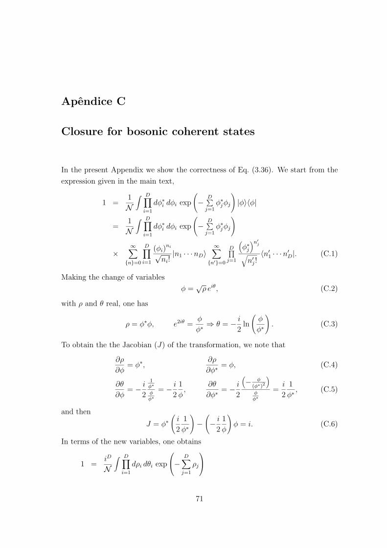
Apendice C
Closure for bosonic coherent states
In the present Appendix we show the correctness of Eq. (3.36). We start from the
expression given in the main text,
1 =1
N∫ D∏
i=1
dφ∗i dφi exp
(− D∑
j=1φ∗jφj
)|φ〉〈φ|
=1
N∫ D∏
i=1
dφ∗i dφi exp
(− D∑
j=1φ∗jφj
)
×∞∑
n=0
D∏
i=1
(φi)ni
√ni!
|n1 · · ·nD〉∞∑
n′=0
D∏j=1
(φ∗j
)n′j
√n′j!
〈n′1 · · ·n′D|. (C.1)
Making the change of variables
φ =√
ρ eiθ, (C.2)
with ρ and θ real, one has
ρ = φ∗φ, e2iθ =φ
φ∗⇒ θ = − i
2ln
(φ
φ∗
). (C.3)
To obtain the the Jacobian (J) of the transformation, we note that
∂ρ
∂φ= φ∗,
∂ρ
∂φ∗= φ, (C.4)
∂θ
∂φ= − i
2
1φ∗φφ∗
= − i
2
1
φ,
∂θ
∂φ∗= − i
2
(− φ
(φ∗)2
)
φφ∗
=i
2
1
φ∗, (C.5)
and then
J = φ∗(
i
2
1
φ∗
)−
(− i
2
1
φ
)φ = i. (C.6)
In terms of the new variables, one obtains
1 =iD
N∫ D∏
i=1
dρi dθi exp
−
D∑
j=1
ρj
71

×∞∑
n=0
D∏
k=1
(√ρk eiθk
)nk
√nk!
|n1 · · ·nD〉∞∑
n′=0
D∏
j=1
(√ρj e−iθj
)n′j
√n′j!
〈n′1 · · ·n′D|
=iD
N∫ D∏
i=1
dρi dθi exp
−
D∑
j=1
ρj
∞∑
n,n′=0
D∏
j=1
√ρj
nj+n′j eiθj(nj−n′j)√
nj!n′j!
× |n1 · · ·nD〉〈n′1 · · ·n′D|. (C.7)
Using the results
2π∫
0
dθ ei(n−n′)θ = 2πδn,n′ ,
∞∫
0
dρ e−ρρn = n!, (C.8)
we get
1 =(2πi)D
N∫ D∏
i=1
dρi exp
−
D∑
j=1
ρj
∞∑
n=0
D∏
j=1
ρnj
j
nj!|n1 · · ·nD〉〈n1 · · ·nD| (C.9)
=(2iπ)D
N∞∑
n=0
|n1 · · ·nD〉〈n1 · · ·nD| = (2iπ)D
N . (C.10)
Therefore, with N = (2πi)D given in Eq. (3.37), one has proven the completeness
relation.
72

Apendice D
Numerical values of the fundamental Grassmann
integrals
For simplicity the following argumentation will be for one generator only. We know
that the l.h.s. of (3.77) is
〈f |g〉 = f ∗0 g0 + f ∗1 g1, (D.1)
but the r.h.s. needs some work before, lets define it as
(f, g) ≡∫
dη∗dη f ∗(η)k(η∗, η)g(η∗)
=∫
dη∗dη(f ∗0 + f ∗1 η)(k0 + k1η∗ + k2η + k3η
∗η)g(η∗)
=∫
dη∗dη(f ∗0 k0 + f ∗0 k1η∗ + f ∗0 k2η
+f ∗0 k3η∗η + f ∗1 k0η + f ∗1 k1ηη∗)g(η∗). (D.2)
Because of we are working with anticommuting variables we are going to impose,
analogously to the derivative, that any variable has to be next to the integral before
to operate
(f, g) =∫
dη∗dη(f ∗0 k0 + f ∗0 k1η∗ + f ∗0 k2η − f ∗0 k3ηη∗ + f ∗1 k0η + f ∗1 k1ηη∗)g(η∗)
=∫
dη∗(f ∗0 k0I0 + f ∗0 k1I0η∗ + f ∗0 k2I1
−f ∗0 k3I1η∗ + f ∗1 k0I1 + f ∗1 k1I1η
∗)g(η∗), (D.3)
where we have defined
I0(η) ≡∫
dη and I1(η) ≡∫
dη η, (D.4)
and beign functions of one generator the I’s are of the form
I(η) = a + bη. (D.5)
73
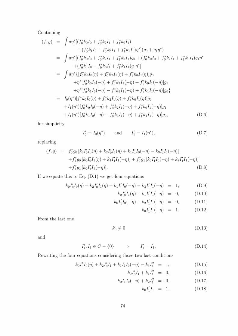
Continuing
(f, g) =∫
dη∗[(f ∗0 k0I0 + f ∗0 k2I1 + f ∗1 k0I1)
+(f ∗0 k1I0 − f ∗0 k3I1 + f ∗1 k1I1)η∗](g0 + g1η
∗)
=∫
dη∗[(f ∗0 k0I0 + f ∗0 k2I1 + f ∗1 k0I1)g0 + (f ∗0 k0I0 + f ∗0 k2I1 + f ∗1 k0I1)g1η∗
+(f ∗0 k1I0 − f ∗0 k3I1 + f ∗1 k1I1)g0η∗]
=∫
dη∗[f ∗0 k0I0(η) + f ∗0 k2I1(η) + f ∗1 k0I1(η)]g0
+η∗[f ∗0 k0I0(−η) + f ∗0 k2I1(−η) + f ∗1 k0I1(−η)]g1
+η∗[f ∗0 k1I0(−η)− f ∗0 k3I1(−η) + f ∗1 k1I1(−η)]g0= I0(η
∗)[f ∗0 k0I0(η) + f ∗0 k2I1(η) + f ∗1 k0I1(η)]g0
+I1(η∗)[f ∗0 k0I0(−η) + f ∗0 k2I1(−η) + f ∗1 k0I1(−η)]g1
+I1(η∗)[f ∗0 k1I0(−η)− f ∗0 k3I1(−η) + f ∗1 k1I1(−η)]g0, (D.6)
for simplicity
I ′0 ≡ I0(η∗) and I ′1 ≡ I1(η
∗), (D.7)
replacing
(f, g) = f ∗0 g0 [k0I′0I0(η) + k2I
′0I1(η) + k1I
′1I0(−η)− k3I
′1I1(−η)]
+f ∗1 g0 [k0I′0I1(η) + k1I
′1I1(−η)] + f ∗0 g1 [k0I
′1I0(−η) + k2I
′1I1(−η)]
+f ∗1 g1 [k0I′1I1(−η)] . (D.8)
If we equate this to Eq. (D.1) we get four equations
k0I′0I0(η) + k2I
′0I1(η) + k1I
′1I0(−η)− k3I
′1I1(−η) = 1, (D.9)
k0I′0I1(η) + k1I
′1I1(−η) = 0, (D.10)
k0I′1I0(−η) + k2I
′1I1(−η) = 0, (D.11)
k0I′1I1(−η) = 1. (D.12)
From the last one
k0 6= 0 (D.13)
and
I ′1, I1 ∈ C − 0 ⇒ I ′1 = I1. (D.14)
Rewriting the four equations considering those two last conditions
k0I′0I0(η) + k2I
′0I1 + k1I1I0(−η)− k3I
21 = 1, (D.15)
k0I′0I1 + k1I
21 = 0, (D.16)
k0I1I0(−η) + k2I21 = 0, (D.17)
k0I′1I1 = 1. (D.18)
74
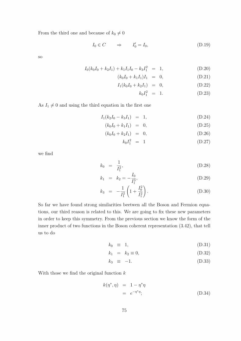
From the third one and because of k0 6= 0
I0 ∈ C ⇒ I ′0 = I0, (D.19)
so
I0(k0I0 + k2I1) + k1I1I0 − k3I21 = 1, (D.20)
(k0I0 + k1I1)I1 = 0, (D.21)
I1(k0I0 + k2I1) = 0, (D.22)
k0I21 = 1. (D.23)
As I1 6= 0 and using the third equation in the first one
I1(k2I0 − k3I1) = 1, (D.24)
(k0I0 + k1I1) = 0, (D.25)
(k0I0 + k2I1) = 0, (D.26)
k0I21 = 1 (D.27)
we find
k0 =1
I21
, (D.28)
k1 = k2 = − I0
I31
, (D.29)
k3 = − 1
I21
(1 +
I20
I21
). (D.30)
So far we have found strong similarities beetwen all the Boson and Fermion equa-
tions, our third reason is related to this. We are going to fix these new parameters
in order to keep this symmetry. From the previous section we know the form of the
inner product of two functions in the Boson coherent representation (3.42), that tell
us to do
k0 ≡ 1, (D.31)
k1 = k2 ≡ 0, (D.32)
k3 ≡ −1. (D.33)
With those we find the original function k
k(η∗, η) = 1− η∗η
= e−η∗η; (D.34)
75

the inner product
〈f |g〉 =∫
dη∗dηf ∗(η)e−η∗ηg(η∗); (D.35)
and then, the closure
I =∫
dη∗dη |η〉e−η∗η〈η|
=∫
dη∗dηe−η∗η|η〉〈η|, (D.36)
it is worth notice that it doesn’t have any normalization factor. Now the integrals
are almost fixed
I0 = 0, (D.37)
I1 = ±1. (D.38)
We are going to choose
I0 =∫
dξ1 = 0 and I1 ≡∫
dξξ = 1, (D.39)
not only for simplicity, but in order to have the same numerical values than of the
derivatives too.
76

Apendice E
Symmetrical term for the exponential in the
partition function
In Section 3.5, Path Integral for bosons and fermions, we mentioned that one can
arrive at two choices for the calculation of the partition function in the ordering of
the Grassmann variables, the second choice is
〈ξm+1|e−εΩ(a†,a)|ξm〉 with m = 0, · · · ,M − 1. (E.1)
We are going to follow the exact same steps. After we introduce the M−1 identities
(3.119)
Z =∫ D∏
i=1
M−1∏
k=0
(dξ∗i,kdξi,k
N
)exp
−
M−1∑
l=0
D∑
j=1
ξ∗j,lξj,l
0∏
m=M−1
〈ξm+1|e−εΩ(a†,a)|ξm〉, (E.2)
we simple order it, and use (3.121)
Z =∫ M−1∏
k=0
D∏
i=1
(dξ∗i,kdξi,k
N
)exp
−
M−1∑
l=0
D∑
j=1
ξ∗j,lξj,l
0∏
m=M−1
exp
D∑
p=1
ξ∗p,m+1ξp,m
e−εΩ¯(ξ∗m+1,ξm)
. (E.3)
Putting together the exponentials, the argument would be
M−1∑
l=0
D∑
j=1
(ξ∗j,l+1 − ξ∗j,l
)ξj,l − εΩ¯(ξ∗l+1, ξl)
= −εM−1∑
l=0
−
D∑
j=1
(ξ∗j,l+1 − ξ∗j,l
)
εξj,l + Ω¯(ξ∗l+1, ξl)
. (E.4)
Replacing it in the partition
Z =∫ M−1∏
k=0
D∏
i=1
(dξ∗i,kdξi,k
N
)e−R(ξ∗,ξ), (E.5)
77

with
R(ξ∗, ξ) ≡ εM−1∑
k=0
−
D∑
j=1
(ξ∗j,k+1 − ξ∗j,k
)
εξj,k + Ω¯(ξ∗k+1, ξk)
. (E.6)
Taking the limit M →∞
limM→∞
Z =∫ ξ(β)
ξ(0)D[ξ∗(τ)ξ(τ)] e−R(ξ∗,ξ), (E.7)
where
∫ ξ(β)
ξ(0)D[ξ∗(τ)ξ(τ)] ≡ lim
M→∞
∫ M−∞∏
‖=′
D∏
〉=∞
(dξ∗〉,‖dξ〉,‖N
), (E.8)
and
R(ξ∗, ξ) ≡∫ β
′dτ
−
D∑
|=∞
(∂ξ∗| (τ)
∂τ
)ξ|(τ) +⊗¯(ξ∗(τ), ξ(τ))
. (E.9)
In which
limM→∞
(ε
M−1∑
l=0
)→
∫ β
0dτ, (E.10)
and
limε→0
(ξ∗j,l − ξ∗j,l−1
)
ε→ ∂ξ∗j (τ)
∂τ. (E.11)
78

Apendice F
The Feynman ordering label technique
In the present Appendix we will explain Feynman’s ordering label technique that
we used in Section 5.4. As remarked there, this technique provides a simplification
on the notation, the final result is not different from the traditional path-ordering
we used in section 5.3. The issue is in some sense trivial, but nevertheless we believe
it is instructive to have an Appendix to to clarify the notation. We shall follow the
original exposition of Feynman in Ref. [39].
The problem of ordering two operators A and B appears because their algebra
is noncommutative in general, that is AB 6= AB. The rules of ordinary algebra and
analysis for ordinary numbers are not directly applicable. For a single operator α,
there is no problem in defining a function of α, like through its power series
A = eα ≡ 1 + α +1
2αα +
1
3!ααα + · · ·
= 1 + α +1
2(α)2 +
1
3!(α)3 + · · · . (F.1)
In these cases the rules of ordinary algebra and analysis apply as for ordinary
numbers. The situation complicates when functions of another operator β, with
αβ 6= βα, are considered. Suppose B = exp β, then in general BA 6= AB, i.e.
BA = eβ eα 6= eβ+α for αβ 6= βα. (F.2)
Let us suppose that β small and expand the exponential to first order in β. The
zeroth order in β is of course exp α, but the first order is neither (exp α)β nor
β(exp α).
Feynman devised a method to indicate the order in which operators are to operate
so as to free them of their noncommutative aspects. Feynman proposed to attach
an index to the operator with the convention that the operator with higher index
operates later. For example, both B1A0 and A0B1 mean BA, i.e. the order of the
indexed operators can be commuted freely as A0 and B1 were ordinary numbers.
79

Thus, if A = exp α and B = exp β, one can safely write
BA = eα0+β1 , (F.3)
since there is only one way to interpret the exponential, namely
eα0+β1 = 1 + α0 + β1 +1
2
(α0 + β1
)2+ · · ·
(F.4)
= 1 + α0 + β1 +1
2
(α2
0 + 2α0β1 + β21
)
(F.5)
= 1 + α + β +1
2
(α2 + 2αβ + β2
)+ · · · . (F.6)
This is the correct answer, since
eα eβ =(1 + α +
1
2α2 + · · ·
) (1 + β +
1
2β2 + · · ·
)
(F.7)
= 1 + β +1
2β2 + α + αβ +
1
2α2 + · · ·
(F.8)
= 1 + α + β +1
2
(α2 + 2αβ + β2
)+ · · · . (F.9)
Let us write the exponential of the sum α + β as
exp(α + β) = limn→∞
[exp
1
n(α + β)
]n
= limn→∞
[1 +
1
n(α + β)
]n
= limn→∞
[1 +
1
n(α + β)
] [1 +
1
n(α + β)
]· · ·
[1 +
1
n(α + β)
]
︸ ︷︷ ︸n times
. (F.10)
In each factor 1+1/n (α+ β) we replace α+ β by αi + βi, with 1 ≤ i ≤ n, and write
exp(α + β) = limn→∞
[1 +
1
n(αn + βn)
] [1 +
1
n(αn−1 + βn−1)
]· · ·
[1 +
1
n(α1 + β1)
]
= limn→∞
[1 +
1
n(αn + βn) +
1
n(αn−1 + βn−1) + · · ·+ 1
n(α1 + β1)
]
= limn→∞ exp
[1
n
n∑
i=1
(αi + βi)
]. (F.11)
80
In the limit of n → ∞, the discrete index becomes continuous i/n → s, 0 ≤ s ≤ 1,
with 1/n → ds, αi → α(s), βi → β(s), and
exp(α + β) = exp∫ 1
0ds [α(s) + β(s)]. (F.12)
As Feynman remarked, it is evident that this expression is correct: calling α(s) +
β(s) = γ(s), with γ a definite operator operating at order s, one has that
exp[∫ 1
0ds γ(s)
]= exp
[∫ 1
0ds γ
], (F.13)
since γ does not need to have the s dependence, it commutes with itself the integral,
and therefore ∫ 1
0ds γ(s) = γ
∫ 1
0ds = γ. (F.14)
The expression in Eq. (F.12) at itself is trivial, but its nontrivial feature is that
the r.h.s. can be manipulated as α(s) and β(s) were ordinary functions of s, since
the order of operations will always be automatically specified by the index. For
example, in particular
exp(α + β) = exp∫ 1
0ds [α(s) + β(s)]
= exp[∫ 1
0ds1 α(s1) +
∫ 1
0ds2 β(s2)
]
=[exp
∫ 1
0ds1 α(s1)
] [∫ 1
0ds2 β(s2)
]. (F.15)
Let us check this for the lowest nontrivial order. The l.h.s. of this expression
gives
exp(α + β) = 1 + α + β +1
2
(α2 + αβ + βα + β2
)+ · · · . (F.16)
The ordering issue here is with respect to the term (αβ + βα)/2 . Let us see how
this ordering appears with the integrals on the r.h.s. of Eq. (F.15). The ordering
comes from the product of integrals∫ 10 ds1 α(s1)
∫ 10 ds2 β(s2), which can be written
as∫ 1
0ds1 α(s1)
∫ 1
0ds2 β(s2) =
∫ 1
0ds1 α(s1)
∫ s1
0ds2 β(s2)
+∫ 1
0ds1 α(s1)
∫ s1
s1
ds2 β(s2). (F.17)
In the first integral on the r.h.s. one has s1 > s2, so that α(s1)β(s2) = αβ and the
value of the integral is∫ 1
0ds1 α(s1)
∫ s1
0ds2 β(s2) = αβ
∫ 1
0ds1
∫ s1
0ds2
81

= αβ∫ 1
0ds1s1
=1
2αβ. (F.18)
In the second integral, one has s2 > s1, then α(s1)β(s2) = βα, and the value of the
integral is∫ 1
0ds1 α(s1)
∫ 0
s1
ds2 β(s2) = βα∫ 1
0ds1
∫ 1
s1
ds2
= βα∫ 1
0ds1(1− s1)
= αβ(1− 1
2
)
=1
2αβ. (F.19)
A case of interest to the present dissertation is when we want to expand exp(α+β)
for β small. Let us consider the expansion to first order in β,
exp(α + β) =[exp
∫ 1
0ds1 α(s1)
] [∫ 1
0ds2 β(s2)
]
≈[exp
∫ 1
0ds1 α(s1)
] (1 +
∫ 1
0ds2 β(s2)
)
= exp∫ 1
0ds1 α(s1) +
[exp
∫ 1
0ds1 α(s1)
] ∫ 1
0ds2 β(s2). (F.20)
The first term is trivial and gives exp α. In the second term, we break the integral
over s1 as[exp
∫ 1
0ds1 α(s1)
]=
[exp
∫ 1
s2
ds1 α(s1)] [
exp∫ s2
0ds1 α(s1)
]. (F.21)
So, we have to consider the ordering of[exp
∫ 1
s2
ds1 α(s1)] [
exp∫ s2
0ds1 α(s1)
]β(s2). (F.22)
The α(s1) in the first factor acts after β(s2) and is for all effects independent of s1,
but α(s1) in the second term is to act before β(s2). So, if we write β(s2) between
both terms and imply the usual convention, the α(s1)’s become independent of s1
in the range from 0 to s2 and one may perform the integrals[exp
∫ 1
0ds1 α(s1)
] ∫ 1
0ds2 β(s2) = [exp α]
∫ 1
0ds [exp(−s)α] β [exp sα]
= eα∫ 1
0ds e−sα β esα. (F.23)
82

That is, we have obtained the result
eα+β = eα[1 +
∫ 1
0ds e−sα β esα + · · ·
], (F.24)
which coincides with Eq. (5.46) to first order.
It is important to note that in a practical calculation, an expression like∫ 10 ds α(s)
standing alone is obviously equal to α, but it is far from trivial when multiplied by
factors involving∫ 10 ds β(s). This means one must consider the complete expression
as a functional of α(s), β(s), etc.
One last remark: if one has
exp[−λ(α + β)], (F.25)
where λ is an ordinary number, Feynman’s formula is
exp[−λ(α + β)] = exp∫ λ
0ds [α(s) + β(s)]
=
[exp
∫ λ
0ds1 α(s1)
] [∫ λ
0ds2 β(s2)
], (F.26)
as can be easily checked.
83

Referencias
[1] J.W. Negele and H. Orland, Quantum Many-Particle Systems, Westview
Press, 1988.
[2] A.L. Fetter and J.D. Walecka, Quantum Theory of Many-Particle-Particle
Systems, McGraw Hill, 1971.
[3] C. Morningstar, The Monte Carlo method in quantum field theory, Lectures
given at the 21st annual Hampton University Graduate Studies (HUGS) Pro-
gram at Jefferson Lab, Newport News, VA, June 5-23, 2006; arXiv:hep-
lat/0702020.
[4] N. Metropolis, A.W. Rosenbluth, M.N. Rosenbluth, A.H. Teller and E. Teller,
J. Chem. Phys. 21, 1087 (1953).
[5] F.A. Berezin, The method of second quantization, Academic Press, 1966.
[6] C. Itzykson and J. B. Zuber, Quantum Field Theory, McGraw-Hill, 1980.
[7] J. Wess and J. Bagger, Supersymmetry and Supergrauity, Princeton University
Press, 1983.
[8] R.L. Stratonovich, Soviet Physics Doklady 2, 416 (1958); J. Hubbard, Phys.
Rev. Lett. 3, 77 (1959).
[9] I.C. Charret, E.V. Correa Silva, S.M. de Souza, O. Rojas Santos, M.T.
Thomaz, and C.E.I. Carneiro, Physica A 264, 204 (1999).
[10] S.M. de Souza and M.T. Thomaz, J. Math. Phys. 32, 3455 (1991).
[11] I.C. Charret, E.V. Correa Silva, S.M. de Souza and M.T. Thomaz, J. Math.
Phys. 36, 4100 (1995).
[12] I.C. Charret, S. M. de Souza and M.T. Thomaz, Braz. J. Phys. 26, 720 (1996).
[13] I.C. Charret, E.V. Correa Silva, S.M. de Souza, O. Rojas Santos, e M.T.
Thomaz, J. Math. Phys. 40, 4944 (1999).
84
[14] P. M. Stevenson, Phys. Rev. D 23, 2916 (1981).
[15] A. Okopinska, Phys. Rev. D 35, 1835 (1987).
[16] G. Krein, R. S. Marques de Carvalho, D. P. Menezes, M. Nielsen and
M. B. Pinto, Eur. Phys. J. A 1, 45 (1998) [arXiv:nucl-th/9709049].
[17] R. L. S. Farias, G. Krein and R. O. Ramos, Phys. Rev. D 78, 065046 (2008)
[arXiv:0809.1449 [hep-ph]].
[18] W. Ketterle and M.W. Zwierlein, Making, probing and understanding ultracold
Fermi gases, International School of Physics ”Enrico Fermi”, Course CLXIV,
Varenna, 20 - 30 June 2006, edited by M. Inguscio, W. Ketterle, and C.
Salomon, IOS Press, 2008; arXiv:0801.2500v1
[19] M.H. Anderson, J.R. Ensher, M.R. Matthews,C.E. Wieman, and E.A. Cornell,
Science 269, 198 (1995); K.B. Davis, M.-O. Mewes, M.R. Andrews,N.J. van
Druten, D.S. Durfee, D.M. Kurn, and W. Ketterle, Phys. Rev. Lett. 75, 3965
(1995).
[20] J. Cubizolles, T. Bourdel, S.J.J.M.F. Kokkelmans, G.V. Shlyapnikov, and C.
Salomon, Phys. Rev. Lett. 91, 240401 (2003).
[21] S. Jochim, M. Bartenstein,A. Altmeyer, G. Hendl, C. Chin, J. Hecker-
Denschlag, and R. Grimm, Phys. Rev. Lett. 91, 240402 (2003) ; C.A. Regal,
M. Greiner, and D.S. Jin, Phys. Rev. Lett. 92, 083201 (2004).
[22] S. Giorgini, L. P. Pitaevskii, and S. Stringari, Rev. Mod. Phys. 80, 1215 (2008).
[23] T. Schaefer and D. Teaney, Nearly Perfect Fluidity: From Cold Atomic Gases
to Hot Quark Gluon Plasmas, [arXiv:0904.3107v2 [hep-ph] 17 Jul 2009]
[24] Atomcool: http://atomcool.rice.edu/ .
[25] CUA: http://cuaweb.mit.edu/Pages/Home.aspx .
[26] D. Lee, Phys. Rev. C 78, 024001 (2008) [arXiv:0803.1280 [nucl-th]].
[27] D. Lee and T. Schafer, Phys. Rev. C 73, 015202 (2006) [arXiv:nucl-
th/0509018].
[28] D. Lee and T. Schafer, Phys. Rev. C 73, 015201 (2006) [arXiv:nucl-
th/0509017].
85
[29] D. Lee, Phys. Rev. B 73, 115112 (2006) [arXiv:cond-mat/0511332].
[30] I. Montvay and G. Munster, Quantum fields on a lattice, Cambridge University
Press, 1997.
[31] H.J. Rothe, Lattice gauge theories: an introduction, World Scientific, 2005 .
[32] B. Bringoltz, Dense hadronic matter in strong coupling lattice gauge theory,
PhD Thesis, Tel Aviv University, 2004; B. Bringoltz and B. Svetitsky, Phys.
Rev. D 68, 034501 (2003).
[33] Ph. de Forcrand and M. Fromm, Nuclear Physics from lattice QCD at strong
coupling, arXiv:0907.1915 [hep-lat].
[34] M. Creutz, Found. Phys. 30, 487 (2000) [arXiv:hep-lat/9905024].
[35] J. Bardeen, L.N. Cooper, and J.R. Schrieffer, Phys. Rev. 108, 1175 (1957).
[36] N.N. Bogoliubov, Sov. Phys.-JETP 7, 41 (1958), J.G. Valatin, Nuovo Cimento
7, 843 (1958).
[37] H. Lipkin, Quantum Mechanics: New Approaches to Selected Topics, Dover,
2001.
[38] X.-J. Liu, H. Hu and P. Drummond, Phys. Rev. A 75, 023614 (2007).
[39] R.P. Feynman, Phys. Rev. 84, 108 (1951).
86