evans and scavia - university of michigan
TRANSCRIPT

Forecasting hypoxia in the Chesapeake Bay and Gulf of Mexico model accuracy precision
and sensitivity to ecosystem change
This article has been downloaded from IOPscience Please scroll down to see the full text article
2011 Environ Res Lett 6 015001
(httpiopscienceioporg1748-932661015001)
Download details
IP Address 741091242
The article was downloaded on 25122010 at 1130
Please note that terms and conditions apply
View the table of contents for this issue or go to the journal homepage for more
Home Search Collections Journals About Contact us My IOPscience
IOP PUBLISHING ENVIRONMENTAL RESEARCH LETTERS
Environ Res Lett 6 (2011) 015001 (11pp) doi1010881748-932661015001
Forecasting hypoxia in the ChesapeakeBay and Gulf of Mexico model accuracyprecision and sensitivity to ecosystemchangeMary Anne Evans1 and Donald Scavia12
1 School of Natural Resources and Environment University of Michigan Ann ArborMI 48109 USA2 Graham Sustainability Institute University of Michigan Ann Arbor MI 48104 USA
E-mail mevansumichedu and scaviaumichedu
Received 25 August 2010Accepted for publication 26 November 2010Published 23 December 2010Online at stacksioporgERL6015001
AbstractIncreasing use of ecological models for management and policy requires robust evaluation ofmodel precision accuracy and sensitivity to ecosystem change We conducted such anevaluation of hypoxia models for the northern Gulf of Mexico and Chesapeake Bay usinghindcasts of historical data comparing several approaches to model calibration For bothsystems we find that model sensitivity and precision can be optimized and model accuracymaintained within reasonable bounds by calibrating the model to relatively short recent 3 yeardatasets Model accuracy was higher for Chesapeake Bay than for the Gulf of Mexicopotentially indicating the greater importance of unmodeled processes in the latter systemRetrospective analyses demonstrate both directional and variable changes in sensitivity ofhypoxia to nutrient loads
Keywords model-data comparison coastal systems nitrogen loading eutrophication
1 Introduction
Ecological models are increasingly moving from heuristic toapplied and this movement requires rigorous analysis andoptimization of accuracy precision and sensitivity to systemchange Ecological systems are subject to sporadic changescaused by internal dynamics (Bronmark et al 2010) shifts indrivers (climate (Scheffer and van Nes 2007) human inputs(Goolsby et al 2001 Rabalais et al 2002a)) invasive species(Higgins and Zanden 2010) and other factors Some ofthese changes can be included in models explicitly but othersare beyond the scope of most modeling activities Theseunmodeled changes and processes are generally parameterizedthrough key model coefficients and because systems changethose parameterizations are subject to change therefore it isimportant for model calibrations to reflect the current state ofthe system
Ecosystems are also subject to relatively high lsquorandomrsquoshort-term variability (eg weather) that does not necessarilyreflect directional change Robust model parameterizationthus also requires sufficiently long time frames to capturethe range of system variability to both detect mean behaviorand undertake reasonable uncertainty analysis There isa potential tension between the goals of providing highaccuracy and high precision and between the challenges ofincorporating information about both random variability andlong-term system changes So it is important to developmodel calibration approaches that optimize model performance(accuracy precision) in the face of systems that are bothundergoing directional change and are highly variable
Models of varying degrees of complexity have beeninformative tools in understanding the controls on hypoxiaoccurrence in river-impacted coastal areas (Pena et al 2010)Hypoxia low oxygen concentrations in bottom waters occurs
1748-932611015001+11$3300 copy 2011 IOP Publishing Ltd Printed in the UK1
Environ Res Lett 6 (2011) 015001 M A Evans and D Scavia
when decomposition rates exceed those of oxygen diffusionand mixing Hypoxia is a widespread and increasingphenomenon (Diaz and Rosenberg 2008 Zhang et al 2010) thatcan lead to widespread ecosystem changes including alteredbiogeochemical cycles (Kemp et al 2005 Turner et al 2008)fish kills (Diaz and Rosenberg 2008) decreased or displacedfish production (Rabalais and Turner 2001) and decreasedvalue to human use through recreation and fisheries harvestlosses (Renaud 1986)
Two major river-impacted coastal hypoxic areas of theUnited States occur in the Gulf of Mexico (GOM) alongthe LouisianandashTexas coasts and in Chesapeake Bay (CB)Hypoxia has been heavily studied in these areas (Justicet al 1993 Bierman et al 1994 Rabalais et al 1994 1998Boesch et al 2001 Rabalais and Turner 2001 Hagy 2002Rabalais et al 2002a 2002c Childs et al 2002 Rabalaiset al 2004 Kemp et al 2005 Rabalais 2006 Walker andRabalais 2006 Scully 2010 etc) due in part to concern overpotential fisheries impacts (Renaud 1986 Rabalais and Turner2001) and management goals have been set to limit hypoxiaseverity Models have been used successfully in both systemsto explore the underlining causes of hypoxia and to makespecific management recommendations (Cerco and Cole 1993Rabalais et al 2002b Justic et al 2003 Scavia et al 2003 Hagyet al 2004 Turner et al 2005 Scavia et al 2006 Turner et al2006 Justic et al 2007 Rabalais et al 2007 Turner et al 2008Greene et al 2009 Penta et al 2009 Wang and Justic 2009Bianchi et al 2010 Liu et al 2010 Liu and Scavia 2010 Penaet al 2010) Models and empirical data indicate that hypoxiain these systems is caused by a combination of nutrient-drivenmostly nitrogen production of phytoplankton organic matterdecomposition freshwater-driven stratification of the water-column and storm mixing Management recommendationshave generally focused on control of nitrogen loading to thesesystems due to evidence that it is an important driver of hypoxiaand its susceptibility to management compared to other driversHowever phosphorus load control has also been addressed(Boesch et al 2001 Environmental Protection Agency (EPA)Science Advisory Board (SAB) 2007 Mississippi RiverGulfof Mexico Watershed Nutrient Task Force 2008)
Both systems have also undergone significant ecosystemchanges in hypoxia sensitivity to nutrient loads over the last30 years such that in both systems the severity of hypoxiafor a given nitrogen load is now approximately twice whatit was in the early 1980s (Hagy et al 2004 Turner et al2008 Liu et al 2010 Liu and Scavia 2010) Ongoingresearch and management scenarios are thus complicated bythe need to account for this varying ecosystem sensitivity andby speculation about how the systems will respond as nutrientloads change Shifts in system sensitivity can appear abruptwhen viewed retrospectively (Hagy et al 2004 EnvironmentalProtection Agency (EPA) Science Advisory Board (SAB)2007 Turner et al 2008 Greene et al 2009 Liu et al 2010)however because of significant interannual variability theycan be impossible to recognize contemporaneously Thisdelayed recognition of sensitivity change is a challenge to bothshort- (annual) and long- (management scenarios) term resultsand highlights the need for models and model calibration
approaches that optimize model performance in changing andhighly variable systems
In this study we test different model calibrationapproaches for fitting similar models of the GOM andCB to subsets of historical data that include systemchanges and periods of high variability A wide range ofmodeling approaches from simple regressions to 3D coupledhydrodynamicndashbiogeochemical and earth system models havebeen applied to hypoxia for both management and scientificinvestigation (Pena et al 2010) More complex models aregenerally able to resolve finer scale ecological mechanismsand provide process based insight Simpler models howeverare often better predictors of system state and have provenvery useful for management applications (Pena et al 2010)Within this range we use a relatively simple mechanisticallybased model that treats estuary and coastal currents as lsquoriversrsquowith point source organic matter loads We selected thismodel because it has proven useful for management guidanceand because the computational simplicity allows the explicitincorporation of uncertainty analysis (Scavia et al 2003 20042006 Scavia and Donnelly 2007 Stow and Scavia 2009 Liuet al 2010 Liu and Scavia 2010) For a description of thismodelrsquos use in the GOM in the context of other modelingapproaches see the recent review by Pena et al (2010)
We test for accuracy precision and model sensitivity tosystem changes by hindcasting parts of the historical datasetWe then compare optimal model calibrations between thesetwo systems and discuss its implications for both ecologicalinterpretation and management Finally we use our optimalcalibrations to forecast outcomes under different nutrientreduction scenarios
2 Methods
21 Models
We use versions of the StreeterndashPhelps (SP) river model(Chapra 1997) developed for CB and the GOM The modelis described in greater depth and its assumptions justified inearlier publications (Scavia et al 2003 2004 2006 Scaviaand Donnelly 2007 Stow and Scavia 2009 Liu et al 2010Liu and Scavia 2010) These models share the same basicstructure but are adapted to each system Both models treat theestuary or coastal current as a lsquoriverrsquo and calculate longitudinalprofiles of dissolved oxygen (DO) concentration downstreamof an organic matter (BOD) point source (described below foreach system) This organic matter point source is assumed tobe proportional to the spring total nitrogen (TN) loading to thesystem with a proportionality constant equal to the product ofthe Redfield carbon to nitrogen ratio the respiration ratio ofoxygen consumption per organic carbon and the dilution ofinputs within the receiving water body Spring TN loads wereused because spring loads are the dominant drivers of hypoxiain these systems (Cerco 1995 Scavia et al 2003 Hagy et al2004 Turner et al 2006)
2
Environ Res Lett 6 (2011) 015001 M A Evans and D Scavia
DO profiles are calculated at steady state for each locationalong the profile DO is calculated by
DO = DOs minus kdBODu F
kr minus kd(eminuskd
xv minus eminuskr
xv ) minus Die
minuskrxv (1)
where DO = dissolved oxygen (mg lminus1) DOs = oxygensaturation (mg lminus1) kd = BOD decay coefficient (1day)kr = reaeration coefficient (1day) BODu = initial BOD(mg lminus1) x = downstream distance (km) F = fractionof BOD sinking below the pycnocline (unitless) Di = theinitial oxygen deficit (mg lminus1) and v = net downstreamadvection (kmday) While in the original SP formulationv represents net downstream advection in this application italso parameterizes the combined effect of horizontal transportand subsequent settling of organic matter from the surfaceTherefore it has no simple physical analog
The length of the hypoxic zone is summed across the partof the profile with DO at hypoxic levels and converted to ameasure of hypoxic area or volume by empirical relationshipsdeveloped from measurements of the hypoxic area or volumein each system (see below) The model was calibrated by fittingpredicted and measured area or volume and minimizing errorterms During calibration each parameter can be assumed tobe either constant across all years or adjusted each year If aparameter is adjusted each year we assume that its variabilityincludes the effects of all unmodeled processes
As in prior applications to CB and the GOM (Stow andScavia 2009 Liu et al 2010 Liu and Scavia 2010) the modelwas calibrated using Bayesian fitting through Markov ChainMonte Carlo methods (Lunn et al 2000 Gill 2002 Gelman andHill 2007) All model calibration was conducted in WinBUGS(version 143) called through R (version 260 R2WinBUGSversion 21-8) using the same methods and inputs describedelsewhere (Stow and Scavia 2009 Liu et al 2010 Liu andScavia 2010) In prior applications of both models either v orF was allowed to vary by year and all other parameters werefit as constants across years or determined from empirical data(see below)
Model application to the two systems differed in fourways
(1) The location of the organic matter point source wasdetermined by the geography and physics of each system InCB summer surface waters flow seaward and bottom watersflow landward The primary nutrient input to the modeledarea of CB is the Susquehanna River at the head of the bayand most hypoxia occurs in the mid-bay region Thus themodel origin and organic matter point source were assignedto the lower end of the mid-bay region (220 km down bay fromthe Susquehanna River mouth) and distance in the model isfollowing the landward flowing bottom water Organic matterloading was based on Susquehanna River spring TN loadingIn the GOM hypoxia occurs below a westward flowing coastalcurrent along the Louisiana and Texas costs Because thereare two main nutrient inputs to the GOM (the Mississippiand Atchafalaya Rivers) we model two organic matter pointsources one at the model origin (Mississippi River) and oneat 220 km down current (Atchafalaya River) Organic matteris proportional to spring TN load with 50 of the Mississippi
River and 100 of the Atchafalaya River TN load assumed tobe entrained in the westward current
(2) The initial oxygen deficit (Di) was assumed to be 0in the GOM because there is little oxygen depletion in waterseast of the delta Di in CB was estimated each year basedon measured bottom-water oxygen concentrations at the modelorigin and a stochastic term based on measurement variation
(3) In CB the reaeration coefficient is known to vary withdistance down estuary (Hagy 2002) Our model uses thisobserved variation in distance (x) and calculates krx = bx Kwhere bx is a location specific constant accounting for spatialvariation (Scavia et al 2006) and K is a fit model parameterscaling reaeration
(4) In CB the volume of water with DO lt 2 mg lminus1 isdetermined each year so the model hypoxia cutoff is set to2 mg lminus1 when determining length (L) and volume (V ) iscalculated using the empirical relationship V = 0003 91L2
(Scavia et al 2006) In the GOM hypoxia is reported asthe area of hypoxic bottom water with measurements takenjust above the sediment water interface Because the modelsimulates the entire sub-pycnocline layer and because availableDO profiles show that when near-bottom DO is 2 mg lminus1average sub-pycnocline DO approaches 3 mg lminus1 the GOMmodel hypoxia cutoff is set to 3 mg lminus1 Hypoxic area (A)is calculated using the empirical relationship A = 38835L(Scavia and Donnelly 2007)
22 Data sources
We use spring total nitrogen (MT TNd) loading data from theUSGS to drive both models Average January through MayTN loads from the Susquehanna River (at Conowingo MDgauging station) are used for CB and May TN loads from theMississippi (at St Francisville) and Atchafalaya (at Melville)Rivers are used for the GOM (USGS 2007 2009 2010)
Model calibrations and tests are conducted usingempirically measured hypoxic area (GOM) or volume (CB)GOM hypoxic area has been interpolated from near-bottomDO measurements collected by shelf-wide cruises in late Julyor early August (Rabalais et al 2002b Rabalais 2009) Cruiseshave been conducted yearly since 1985 with the exception of1989 Because the measured hypoxic area was potentiallyimpacted by tropical storms in 1996 1998 2003 and 2005 weremoved these years from both our calibration and test datasets(see Turner et al 2008) because the model is incapable ofaccounting for these extreme conditions Such tropical stormscan disrupt water-column stratification mixing oxygenatedwater downward and thus temporarily break the link betweenproduction and hypoxia observed in non-storm years CBhypoxic volume is determined from DO profiles taken onfour cruises in July and August each year since 1984 andsporadically before then (Hagy et al 2004 Chesapeake BayProgram (CBP) 2008) We use the July CBP cruise data fromthe consistent record since 1984 for model calibration andtesting
Initial oxygen deficit (Di) for CB was based on averageJuly bottom-water oxygen concentration measured at stationsin the mid-bay region (Scavia et al 2006 Chesapeake Bay
3
Environ Res Lett 6 (2011) 015001 M A Evans and D Scavia
Program (CBP) 2008) The difference between saturated andmeasured oxygen concentration was used for mean Di incalibration years For hindcasts and forecasts Di was drawnfrom a normal distribution with average and standard deviationequal to that in the measured calibration data
23 Hindcast and forecast tests
We tested several model calibration algorithms to optimizemodel performance Each test used a calibration datasetand a test dataset Model performance was measured byassessing precision accuracy robustness and sensitivity tosystem change although some tests focus on a subset ofthese measures Precision was assessed as the size of thecoefficient of variation and the 95 credible interval (CI) ofthe model prediction Accuracy was assessed as the percentageof observations in the test dataset that fell within the 95 CI ofthe model prediction It is expected that this value could differfrom 95 because the test dataset contains observations foryears that are not included in the model calibration and thus themodel is predicting outside its statistical sample Robustnesswas based on the impact of individual years in the calibrationdata set on calibrated parameter values Sensitivity to systemchange was assumed to be maximized when few recent yearsof calibration data were used because averaging across largernumbers of data points decreases the impact of any given pointon the average
To test the impact of increasing the number of yearsin the calibration set on model precision and robustness(Test 1) calibrations began with the first three years of dataand we progressively added years for successive calibrations(calibration dataset) To test precision we used each calibratedmodel to predict hypoxia for each year in the full dataset (testdataset) and the average CV and 95 CI were calculated Totest robustness we examined variation in parameter valuesover time from each calibration test Model accuracy wasquantified by calculating the percentage of observed hypoxicareas or volumes that fell within the modelrsquos 95 CI for thatyearrsquos prediction We repeated this test (Test 2) beginning withthe three most recent years and adding years in reverse order
Because the above comparisons are confounded byoverlap between the calibration and test datasets they wereused only to narrow the range of years for which a morecomplete test was conducted In these tests of accuracyforecasts were conducted using 3 5 and 7 year windows ofcalibration data (Test 3 range selected based on the resultsof Tests 1 and 2 see below) Precision was quantified bythe CV of the hypoxia forecast in the year following eachcalibration and the average of these CVs across all calibrationsusing the same window size The accuracy of these calibrationswas tested by forecasting hypoxia in the year following eachcalibration window and calculating the percentage of observedhypoxic areas or volumes that fell within the forecastrsquos 95 CIacross all calibrations using that window (test dataset)
To prepare for forecasts where all model coefficients areto be held constant we tested two methods of parametercalibration In prior work with this model (Liu et al 2010 Liuand Scavia 2010) v was estimated as the year-specific term vi
and then forecasts used the mean and standard deviation of vi
through time ignoring the Bayesian fit parameter distributionWe compared this approach with one that estimated allparameters (including v) as constant distributions throughtime such that forecasts could be conducted directly from thecalibrated distributions (Test 4) For both methods (using vi
and v) in CB the parameter Di which is not calibrated butcalculated from observed values for calibration years wasestimated using the average and variation in the previouslyobserved values
24 Response curves
Response curves of predicted hypoxic area or volume versusspring TN load were constructed in the same way as hindcastsand forecasts but using evenly spaced spring TN loadsspanning the observed range rather than exact historical loads(Scavia et al 2006 Liu et al 2010 Liu and Scavia 2010) Asin prior publications (Liu et al 2010 Liu and Scavia 2010)response curves were constructed using 50 CIs to betterconstrain conditions in typical or average years
3 Results
31 Full dataset calibration
When the model is fit to the entire CB and GOM datasetsallowing vi to vary in each year and then averaging vi forhindcasts hindcasting accuracy is high (100 and 80 ofthe observations are within the 95 CI of the hindcastrespectively see right-most symbols associated with the fulldataset in figures 1(a) and (c)) These percentages differ from95 because of additional variability added to the model whenthe parameter vi and the parameter Di in the CB model areaveraged across years Model precision as measured by theCV of the predicted hypoxic region is better for CB (33) thanfor the GOM (41) (see right-most symbols associated withthe full dataset in figures 1(a) and (c)) Model parameters havemean values of F = 091 kd = 014 K = 058 vA = 25(where A indicates the average across years) DA = 12 forCB and F = 051 kd = 0006 kr = 0012 vA = 064for the GOM (see right-most symbols associated with the fulldataset in figures 1(b) and (d)) These values are consistentwith previously published model calibrations and as in priorcalibrations estimated process rates based on these parametersare consistent with observed rates (Scavia et al 2006 Scaviaand Donnelly 2007 Liu et al 2010 Liu and Scavia 2010)
32 Effect of number of years in the calibration
The precision and accuracy of the models calibrated to the fulldatasets represent a goal for calibrations using sub-datasetsHowever they may not represent the best overall modelcalibration because using the full dataset ignores temporaltrends and regime shifts within the system and thus sacrificesmodel sensitivity to system change It also confoundscalibration and test datasets causing a possible overestimationof model accuracy in predicting novel conditions So wetested model performance by calibrating to subsets of data
4
Environ Res Lett 6 (2011) 015001 M A Evans and D Scavia
Figure 1 (Test 1) Average CV of predicted hypoxic volume or area and observations in 95 CI using (a) a test dataset of Chesapeake Bayhypoxic volume from 1984ndash2008 and calibration datasets of increasing numbers of years starting in 1984 and (c) a test dataset of Gulf ofMexico hypoxic area from 1985ndash2009 and calibration datasets of increasing numbers of years starting in 1985 Parameter estimates (panels(b) and (d) means with 50 CI bars for vA) corresponding to the model calibrations used in panels (a) and (c) Note that results fromcalibrating to the full datasets are shown as the right-most symbols in each graph
with increasing number of years Beginning at the start ofeach dataset (Test 1) adding years causes a rapid improvementfor the CB model performance in both precision and accuracyuntil about 5 years of data are used (figure 1(a)) Beyondthis point precision and accuracy asymptote toward values ofthe full dataset Similarly CB parameter values were highlyvariable in the beginning until about 5 years of data wereused (figure 1(b)) Beyond 5 years there was little change invalues despite known changes in system behavior indicatingthat model calibration to long datasets loses sensitivity tothese changes These same patterns of precision accuracyand parameter variability were observed when calibration wasstarted using the three most recent years and adding years inreverse order (Test 2 data not shown) Thus using about 5years of calibration data seems to offer an optimal combinationof model precision accuracy and robustness while avoiding aloss of sensitivity to system change in this system
Determining optimal calibration for the GOM involvesa greater compromise between precision and sensitivity Asin CB adding calibration years (Test 1) causes a rapidimprovement in model precision and accuracy (figure 1(c))However precision and accuracy continue to improve untilabout 15 years of calibration data The model also maintainedmore sensitivity to system change with the addition ofcalibration years for longer datasets than the CB model(figure 1(d)) Parameter values especially F and kr continue tochange as years are added up to at least 15 years of calibrationdata When calibration started using the three most recentyears and years were added in reverse order (Test 2 data notshown) model accuracy was high (100 of observations inthe 95 CI) using even 3 years of data and remained at thislevel as years were added Model precision improved quicklyuntil about 5 years and then saturated and parameter valuesvaried in a similar pattern Though results were more mixed
5
Environ Res Lett 6 (2011) 015001 M A Evans and D Scavia
Figure 2 (Test 3) (a) CV of predicted hypoxic volume in CB for the year following each 3 5 and 7 year calibration period (b) Parameterestimates with error bars showing the 50 CI of average v over the 3 year calibration period
Figure 3 (Test 3) (a) CV of predicted hypoxic area in the GOM for the year following each 3 5 and 7 year calibration period (b) Parameterestimates with error bars showing the 50 CI of average v over the 3 year calibration period
for the GOM with continued improvement in model precisionand accuracy beyond the first 5 years of calibration data in theforward though not the backward calibration tests we decidedto further test models using 5 years of calibration data becauseusing 15 or 20 years lost sensitivity to system changes whichhave been observed on shorter time scales (Turner et al 2008Liu et al 2010)
33 Moving window calibrations case 1mdashaveraging vi
Previous applications of this model estimated vi for each yearin a calibration dataset and then averaged it for forecasts Sowe first test the moving window calibrations (Test 3) withthis method and then compare it below to the case where v
is estimated as a constant over the calibration widow period(Test 4) Tests with 3 5 and 7 year moving windows
showed little difference in precision (CV) when forecastingCB (figure 2(a)) or GOM (figure 3(a)) hypoxia in the yearfollowing the calibration window and no overall improvementin precision using larger windows A change in precision couldindicate over or under fitting the model but this does not seemto be taking place For all window sizes parameter valueschanged over time however parameter variability was highestusing the smallest (3 year) window (figures 2(b) and 3(b))This increased variability indicates higher model sensitivityto system state because more of the underlying variability isreflected in the parameters Model accuracy was high for allwindow sizes in CB and decreases with window size in theGOM In CB the per cent of observations in the 95 CI is100 95 and 100 for the 3 5 and 7 year calibrationperiods respectively compared to 93 80 and 73 forthese calibrations in the GOM Thus the results support theuse of a 3 year moving window
6
Environ Res Lett 6 (2011) 015001 M A Evans and D Scavia
Figure 4 (Test 4) (a) CV of predicted hypoxic volume in CB for the year following each 3 5 and 7 year calibration period (b) Parameterestimates for the 3 year calibration period (c) Forecast hypoxic volume (black line forecast mean gray dotted lines forecast 95 CI) andobserved hypoxic volume (black dots) for each forecast year using the 3 year calibration period
Compared to using the full dataset 3 year moving windowcalibrations resulted in the same accuracy for CB (100) andimproved accuracy for GOM (95 versus 80 of observationswithin the 95 CI) Average model precision (CV) for the3 year moving window calibration was slightly poorer in CB(39 versus 33) but was slightly improved in the GOM(30 versus 41) Using a moving window allows themodel precision to vary over time based on recent systemvariability Precision is higher (lower CV) during periods ofsystem stability such as the late 1990s in the GOM and lower(higher CV) following regime shifts (figure 3(a))
34 Moving window calibrations case 2mdashconstant v
Fitting vi for each year and then averaging it for forecastsintroduces arbitrary variation into the model As an alternativewe tested moving window calibrations of 3 5 and 7 yearsfitting all parameters including v as constants (Test 4)
With 3 5 and 7 year moving window calibrations CBhypoxia forecast accuracy is lower than expected Accuracy ishighest for the 3 year window and decreases with increasing
window size (82 70 and 68 of observed hypoxicvolume were within the model 95 CI figure 4(c) comparesforecast and observed hypoxia for the 3 year moving windowcalibration) There was very little difference in precision (CV)among window sizes (figure 4(a)) and no overall improvementin precision using larger windows For all window sizesparameter values changed over time however as in prior testsparameter variability was highest using the smallest (3 year)window (figure 4(b)) indicating the highest model sensitivityto system state
Test for the GOM resulted in lower accuracy with 7368 and 46 of the observed hypoxic areas within themodelrsquos 95 CI for 3 5 and 7 year windows respectively(figure 5(c) compares forecast and observed hypoxia for the3 year moving window calibration) There was very littledifference in precision (CV) among window sizes (figure 5(a))no overall improvement in precision using larger windows andparameter values changed over time with the highest variabilityassociated with the smallest (3 year) window (figure 5(b))
The CV of predicted hypoxic area or volume varies withtime in all moving window calibrations However the average
7
Environ Res Lett 6 (2011) 015001 M A Evans and D Scavia
Figure 5 (Test 4) (a) CV of predicted hypoxic area in the GOM for the year following each 3 5 and 7 year calibration period with allparameters treated as constants In 2000 CV of predicted hypoxic area was 98 45 and 54 for the 3 5 and 7 year calibrationperiods respectively and is not graphed (b) Parameter estimates for the 3 year calibration period (c) Forecast hypoxic area (black lineforecast mean gray dotted lines forecast 95 CI) and observed hypoxic area (black dots) for each forecast year using the 3 year calibrationperiod
CV is improved by calibrating with a constant v in bothsystems Using the 3 year window the CV for CB is improvedfrom 39 to 33 and for GOM from 30 to 18 comparedto moving window tests averaging vi This is a substantialimprovement in model precision This increase in modelprecision is accompanied by a decrease in model accuracyHowever because the increased variability introduced intothe model by averaging year-specific vi is not related to aspecific mechanism or known ecological process the lowerforecasting accuracy is likely a better representation of truemodel performance The SP model is a vast simplificationof nature and the accuracy cost of using this model (95 minus82 = 13 for CB and 22 for the GOM) reflect unmodeledvariation in these systems
4 Discussion
The dataset for the GOM included years in three distinct andpreviously observed system states with varying sensitivity to
hypoxia formation (Environmental Protection Agency (EPA)Science Advisory Board (SAB) 2007 Turner et al 2008Greene et al 2009 Liu et al 2010) Similar changes in systemstate have been observed in CB however data limitationsprevented us from including the historic CB system state(Hagy et al 2004 Liu and Scavia 2010) in the current modeltests Model accuracy was poorer for the GOM than forCB and one of the reasons could be the attempt to calibratethe model across multiple system states Including multiplestates is minimized when using short calibration windowsand improved model accuracy in the shortest windows are aresult GOM model accuracy for the 3 year moving windowcalibration fitting v as a constant is further improved to 78when excluding calibrations that overlap more than one systemstate Though such exclusions can only be identified postfacto this further supports use of shorter calibration windowsto minimize including multiple system states
Initial comparisons adding years to the calibrationdataset starting from the oldest (figure 1) or most recent(data not shown) data indicated that 5 or more years
8
Environ Res Lett 6 (2011) 015001 M A Evans and D Scavia
Figure 6 Hypoxia response curves for CB and the GOM based on years early in the historic record and recent years The year ranges cited ineach legend are the years in the respective calibration datasets Solid lines show the average forecast response and dotted lines show the 50CI of forecast response
of calibration data were needed to optimize precision andaccuracy However more extensive comparisons using 3 5and 7 year calibration datasets and employing more robustaccuracy measures (by forecasting only the year following acalibration window) show that model performance is optimizedwith 3 year calibrations These tests showed less of a tradeoffbetween model precision and accuracy than was expectedModel precision did not differ among window lengths in anycomparison and in fitting either year-specific or constant vModel accuracy was either higher in the shortest window ordid not change with window size As expected the shortestwindow calibrations were the most adaptive to system changeThis responsiveness is seen in both the improved modelaccuracy in the changing GOM and in increased parametervariability in both systems
The tradeoff between precision and accuracy existed forboth models calibrated using year-specific or constant v Webelieve that fitting and averaging year-specific vi introduces anartifact that improves model accuracy by arbitrarily reducingprecision Thus we propose that the optimal calibration forannual forecasting is to use a rather short (3 year) recentdataset treating all parameters as constants
41 Forecasts
Using the 3 year window calibrations we developed loadndashhypoxia response curves for CB and the GOM for differentperiods in the historical record (figure 6) The GOM hasundergone two shifts in sensitivity between the earliest (1986ndash8) and most recent (2005ndash7) calibration periods and theresulting increase in sensitivity can be seen across the TNrange
Though the primary CB regime shift appears to haveoccurred before the start of our dataset (Hagy et al 2004 Kempet al 2005 Scavia et al 2006 Conley et al 2009) CB appearsto be undergoing a gradual increase in sensitivity to nutrient
loads from 1983 through at least 2005 (Liu and Scavia 2010Scully 2010) This increasing sensitivity is reflected in ourparameter estimates (figure 4(b)) and in response curves using1988ndash90 and 2002ndash4 calibration datasets (figure 6) Betweenthese periods hypoxia sensitivity increased especially at highTN loads Parameter values for recent years trend back towardand even beyond those earlier in the dataset Accordinglythe most recent (2005ndash2007) response curve shows decreasedsensitivity At high TN loads the curve resembles the 1988ndash90 lsquolow sensitivityrsquo case and it appears to have even lowersensitivity at lower TN loads
These changes are driven mostly by changes in theparameters F v K and Di F and v increase between the firsttwo periods and then decrease again before the final periodSensitivity analyses (not shown) indicate that increases in Ftend to increase sensitivity at all TN loads while increases inv increases sensitivity more at high TN loads At the sametime K decreased between the first two time periods whileremaining relatively unchanged between the second and thirdLike increases in v decreases in K tend to increase sensitivityat high TN loads Finally the measured parameter Di remainedconstant between the first two periods but decreased betweenthe second and third Decreases in Di lead to decreases insensitivity at low TN loads This measured decrease in DOdeficit in recent years may indicate a release from oxygen stressfurther down bay
Using models calibrated with the three most recent yearsor in the case of the GOM the three most recent yearsthat were not impacted by severe tropical storms providesa consistent method for annual forecasts that is relativelyrobust to regime shifts and changes in system sensitivityHowever changes in system sensitivity still pose a significantchallenge for developing long-term scenariosmdashthat is insetting nutrient load targets which response curve is mostappropriate Such long-term forecasts require assumptionsabout the future system sensitivity to hypoxia formation Will
9
Environ Res Lett 6 (2011) 015001 M A Evans and D Scavia
the system continue to follow the most recent curve will itrevert to a former sensitivity (as may be happening in CB) orwill it become even more sensitive We suggest this publicpolicy challenge is best met with ensemble modeling usingthe family of response curves with curve selection weightedbased on expert judgment and acceptable risk For exampleif a given hypoxia level were deemed ecologically or sociallyunacceptable any response curve that predicted hypoxia abovethis level at certain nutrient loadings could be weighted higherover that loading range based on the precautionary principleAlternately evidence of system recovery to a lower sensitivitystate could shift the weighting of curves toward those withlower sensitivity while still maintaining some weight on otherobserved curves
The model presented here is primarily focused onforecasts of interest for hypoxia management and has also beenused to explore system level trends in hypoxia sensitivity (Liuet al 2010) Both simpler and more complex models have alsobeen applied to the GOM and CB systems and each modeltype yields different insights into the physical watershedand biological controls of hypoxia as well as its impacts onindividual organisms food-webs and biogeochemistry (Penaet al 2010)
5 Conclusions
The forecasting ability of a simple hypoxia model withBayesian incorporation of parameter uncertainty and variabil-ity for GOM and CB was optimized by calibration to short(3 year) recent datasets This calibration window approachwas used to assess the tradeoff between incorporating adequatesystem variability into model parameterization and the abilityto track gradual (in CB) and abrupt (in the GOM) ecosystemchanges in hypoxia sensitivity to nutrient loads We proposeuse of this moving window calibration method for future short-term (annual) forecasts The underlying changes in systemsensitivity pose a great challenge to the long-term forecastingand additional work using Bayesian weighting among familiesof models or incorporation of more complex model featurescoupled with climate models is likely needed
Acknowledgments
This work is contribution number 136 of the CoastalHypoxia Research Program and was supported in part bygrant NA05NOS4781204 from NOAArsquos Center for SponsoredCoastal Ocean Research and by the University of MichiganGraham Sustainability Institute We appreciate the insight andadvice provided by Yong Liu
References
Bianchi T S DiMarco S F Cowan J H Hetland R D Chapman PDay J W and Allison M A 2010 The science of hypoxia in theNorthern Gulf of Mexico a review Sci Total Environ408 1471ndash84
Bierman V J Hinz S C Zhu D W Wiseman W J Rabalais N N andTurner R E 1994 A preliminary mass-balance model of primaryproductivity and dissolved-oxygen in the Mississippi riverplume inner Gulf shelf region Estuaries 17 886ndash99
Boesch D F Brinsfield R B and Magnien R E 2001 Chesapeake Bayeutrophication scientific understanding ecosystem restorationand challenges for agriculture J Environ Quality 30 303ndash20
Bronmark C Brodersen J Chapman B B Nicolle A Nilsson P ASkov C and Hansson L A 2010 Regime shifts in shallow lakesthe importance of seasonal fish migration Hydrobiologia646 91ndash100
Cerco C F 1995 Response of Chesapeake Bay to nutrient loadreductions J Environ Eng 121 298ndash310
Cerco C F and Cole T 1993 3-dimensional eutrophication model ofChesapeake Bay ASCE J Environ Eng 119 1006ndash25
Chapra S C 1997 Surface Water-Quality Modeling (New YorkMcGraw-Hill)
Chesapeake Bay Program (CBP) 2008 unpublished dataChilds C R Rabalais N N Turner R E and Proctor L M 2002
Sediment denitrification in the Gulf of Mexico zone of hypoxiaMar Ecol Prog Ser 240 285ndash90
Childs C R Rabalais N N Turner R E and Proctor L M 2003Sediment denitrification in the Gulf of Mexico zone of hypoxiaMar Ecol Prog Ser 247 310 (erratum)
Conley D J Carstensen J Vaquer-Sunyer R and Duarte C M 2009Ecosystem thresholds with hypoxia Hydrobiologia 629 21ndash9
Diaz R J and Rosenberg R 2008 Spreading dead zones andconsequences for marine ecosystems Science 321 926ndash9
Environmental Protection Agency (EPA) Science Advisory Board(SAB) 2007 Hypoxia in the Gulf of Mexico (available online athttpwwwepagovsabpanelshypoxia adv panelhtm)(accessed June 2010)
Gelman A and Hill J 2007 Data Analysis Using Regression andMultilevelHierarchical Models (New York CambridgeUniversity Press)
Gill J 2002 Bayesian Methods A Social and Behavioral SciencesApproach (Boca Raton FL Chapman and HallCRC)
Goolsby D A Battaglin W A Aulenbach B T and Hooper R P 2001Nitrogen input to the Gulf of Mexico J Environ Quality30 329ndash36
Greene R M Lehrter J C and Hagy J D 2009 Multiple regressionmodels for hindcasting and forecasting midsummer hypoxia inthe Gulf of Mexico Ecol Appl 19 1161ndash75
Hagy J D 2002 Eutrophication hypoxia and trophic transferefficiency in Chesapeake Bay PhD University of Maryland
Hagy J D Boynton W R Keefe C W and Wood K V 2004 Hypoxiain Chesapeake Bay 1950ndash2001 long-term change in relation tonutrient loading and river flow Estuaries 27 634ndash58
Higgins S N and Zanden M J V 2010 What a difference a speciesmakes a meta-analysis of dreissenid mussel impacts onfreshwater ecosystems Ecol Monographs 80 179ndash96
Justic D Bierman V J Scavia D and Hetland R D 2007 ForecastingGulfrsquos hypoxia the next 50 years Estuaries Coasts30 791ndash801
Justic D Rabalais N N and Turner R E 2003 Simulated responses ofthe Gulf of Mexico hypoxia to variations in climate andanthropogenic nutrient loading J Mar Syst 42 115ndash26
Justic D Rabalais N N Turner R E and Wiseman W J 1993 Seasonalcoupling between riverborne nutrients net productivity andhypoxia Mar Pollut Bull 26 184ndash9
Kemp W M et al 2005 Eutrophication of Chesapeake Bay historicaltrends and ecological interactions Mar Ecol Prog Ser303 1ndash29
Liu Y Evans M A and Scavia D 2010 Gulf of Mexico hypoxiaexploring increasing sensitivity to nitrogen loads Environ SciTechnol 44 5836ndash41
Liu Y and Scavia D 2010 Analysis of the Chesapeake Bay hypoxiaregime shift insights from two simple mechanistic modelsEstuaries Coasts 33 629ndash39
Lunn D J Thomas A Best N and Spiegelhalter D 2000WinBUGSmdasha Bayesian modeling framework conceptsstructure and extensibility Stat Comput 10 325ndash37
10
Environ Res Lett 6 (2011) 015001 M A Evans and D Scavia
Mississippi RiverGulf of Mexico Watershed Nutrient TaskForce 2008 Gulf Hypoxia Action Plan 2008 for ReducingMitigating and Controlling Hypoxia in the Northern Gulf ofMexico and Improving Water Quality in the Mississippi RiverBasin (Washington DC USEPA Office of Wetlands Oceansand Watersheds) (Action Plan available at wwwepagovowow keepmsbasinactionplanhtm)
Pena M A Katsev S Oguz T and Gilbert D 2010 Modeling dissolvedoxygen dynamics and hypoxia Biogeosciences 7 933ndash57
Penta B et al 2009 Using coupled models to study the effects of riverdischarge on biogeochemical cycling and hypoxia in thenorthern Gulf of Mexico OCEANS 2009 MTSIEEEBiloxi-Marine Technology for our Future Global and LocalChallenges (New York NY IEEE) pp 1ndash7 (available fromhttpieeexploreieeeorgstampstampjsptp=amparnumber=5422347ampisnumber=5422059)
Rabalais N N 2009 personal communicationRabalais N N 2006 Oxygen depletion in the Gulf of Mexico adjacent
to the Mississippi river Gayana (Concepc) 70 73ndash8Rabalais N N Atilla N Normandeau C and Turner R E 2004
Ecosystem history of Mississippi river-influenced continentalshelf revealed through preserved phytoplankton pigments MarPollut Bull 49 537ndash47
Rabalais N N and Turner R E 2001 Coastal Hypoxia Consequencesfor Living Resources and Ecosystems (Washington DCAmerican Geophysical Union)
Rabalais N N Turner R E Dortch Q Justic D Bierman V J andWiseman W J 2002a Nutrient-enhanced productivity in thenorthern Gulf of Mexico past present and futureHydrobiologia 475 39ndash63
Rabalais N N Turner R E and Scavia D 2002b Beyond science intopolicy Gulf of Mexico hypoxia and the Mississippi riverBioscience 52 129ndash42
Rabalais N N Turner R E Sen Gupta B K Boesch D FChapman P and Murrell M C 2007 Hypoxia in the northernGulf of Mexico does the science support the plan to reducemitigate and control hypoxia Estuaries Coasts 30 753ndash72
Rabalais N N Turner R E and Wiseman W J 2002c Gulf of Mexicohypoxia aka lsquoThe dead zonersquo Annu Rev Ecol Syst 33 235ndash63
Rabalais N N Turner R E Wiseman W J and Dortch Q 1998Consequences of the 1993 Mississippi river flood in the Gulf ofMexico Regul Rivers-Res Manag 14 161ndash77
Rabalais N N Wiseman W J and Turner R E 1994 Comparison ofcontinuous records of near-bottom dissolved-oxygen from thehypoxia zone along the Louisiana coast Estuaries 17 850ndash61
Renaud M L 1986 Hypoxia in Louisiana coastal waters during1983mdashimplications for fisheries Fishery Bull 84 19ndash26(available at httpfishbullnoaagov841renaudpdf)
Scavia D and Donnelly K A 2007 Reassessing hypoxia forecasts forthe Gulf of Mexico Environ Sci Technol 41 8111ndash7
Scavia D Justic D and Bierman V J 2004 Reducing hypoxia in theGulf of Mexico advice from three models Estuaries 27 419ndash25
Scavia D Kelly E L A and Hagy J D 2006 A simple model forforecasting the effects of nitrogen loads on Chesapeake Bayhypoxia Estuaries Coasts 29 674ndash84
Scavia D Rabalais N N Turner R E Justic D and Wiseman W J 2003Predicting the response of Gulf of Mexico hypoxia to variationsin Mississippi river nitrogen load Limnol Oceanogr 48 951ndash6
Scheffer M and van Nes E H 2007 Shallow lakes theory revisitedvarious alternative regimes driven by climate nutrients depthand lake size Hydrobiologia 584 455ndash66
Scully M E 2010 The importance of climate variability towind-driven modulation of hypoxia in Chesapeake Bay J PhysOceanogr 40 1435ndash40
Stow C A and Scavia D 2009 Modeling hypoxia in the ChesapeakeBay ensemble estimation using a Bayesian hierarchical modelJ Mar Syst 76 244ndash50
Turner R E Rabalais N N and Justic D 2006 Predicting summerhypoxia in the northern Gulf of Mexico riverine N P and Siloading Mar Pollut Bull 52 139ndash48
Turner R E Rabalais N N and Justic D 2008 Gulf of Mexico hypoxiaalternate states and a legacy Environ Sci Technol 42 2323ndash7
Turner R E Rabalais N N Swenson E M Kasprzak M andRomaire T 2005 Summer hypoxia in the northern Gulf ofMexico and its prediction from 1978 to 1995 Mar Environ Res59 65ndash77
USGS 2007 Chesapeake Bay River Input Monitoring ProgramLoads (available online at httpvawaterusgsgovchesbayRIMPloadshtml) (accessed 10 May 2010)
USGS 2009 Streamflow and Nutrient Delivery to the Gulf of Mexico(available online at httptoxicsusgsgovhypoxiamississippiflux estsdeliveryindexhtml) (accessed 14 June 2010)
USGS 2010 Streamflow and Nutrient Delivery to the Gulf of Mexicofor October 2009 to May 2010 (Preliminary) (available onlineat httptoxicsusgsgovhypoxiamississippioct junindexhtml) (accessed 20 June 2010)
Walker N D and Rabalais N N 2006 Relationships among satellitechlorophyll a river inputs and hypoxia on the Louisianacontinental shelf Gulf of Mexico Estuaries Coasts 29 1081ndash93
Wang L X and Justic D 2009 A modeling study of the physicalprocesses affecting the development of seasonal hypoxia overthe inner LouisianandashTexas shelf circulation and stratificationCont Shelf Res 29 1464ndash76
Zhang J et al 2010 Natural and human-induced hypoxia andconsequences for coastal areas synthesis and futuredevelopment Biogeosciences 7 1443ndash67
11
- 1 Introduction
- 2 Methods
-
- 21 Models
- 22 Data sources
- 23 Hindcast and forecast tests
- 24 Response curves
-
- 3 Results
-
- 31 Full dataset calibration
- 32 Effect of number of years in the calibration
- 33 Moving window calibrations case 1---averaging vi
- 34 Moving window calibrations case 2---constant v
-
- 4 Discussion
-
- 41 Forecasts
-
- 5 Conclusions
- Acknowledgments
- References
-

Environ Res Lett 6 (2011) 015001 M A Evans and D Scavia
Program (CBP) 2008) The difference between saturated andmeasured oxygen concentration was used for mean Di incalibration years For hindcasts and forecasts Di was drawnfrom a normal distribution with average and standard deviationequal to that in the measured calibration data
23 Hindcast and forecast tests
We tested several model calibration algorithms to optimizemodel performance Each test used a calibration datasetand a test dataset Model performance was measured byassessing precision accuracy robustness and sensitivity tosystem change although some tests focus on a subset ofthese measures Precision was assessed as the size of thecoefficient of variation and the 95 credible interval (CI) ofthe model prediction Accuracy was assessed as the percentageof observations in the test dataset that fell within the 95 CI ofthe model prediction It is expected that this value could differfrom 95 because the test dataset contains observations foryears that are not included in the model calibration and thus themodel is predicting outside its statistical sample Robustnesswas based on the impact of individual years in the calibrationdata set on calibrated parameter values Sensitivity to systemchange was assumed to be maximized when few recent yearsof calibration data were used because averaging across largernumbers of data points decreases the impact of any given pointon the average
To test the impact of increasing the number of yearsin the calibration set on model precision and robustness(Test 1) calibrations began with the first three years of dataand we progressively added years for successive calibrations(calibration dataset) To test precision we used each calibratedmodel to predict hypoxia for each year in the full dataset (testdataset) and the average CV and 95 CI were calculated Totest robustness we examined variation in parameter valuesover time from each calibration test Model accuracy wasquantified by calculating the percentage of observed hypoxicareas or volumes that fell within the modelrsquos 95 CI for thatyearrsquos prediction We repeated this test (Test 2) beginning withthe three most recent years and adding years in reverse order
Because the above comparisons are confounded byoverlap between the calibration and test datasets they wereused only to narrow the range of years for which a morecomplete test was conducted In these tests of accuracyforecasts were conducted using 3 5 and 7 year windows ofcalibration data (Test 3 range selected based on the resultsof Tests 1 and 2 see below) Precision was quantified bythe CV of the hypoxia forecast in the year following eachcalibration and the average of these CVs across all calibrationsusing the same window size The accuracy of these calibrationswas tested by forecasting hypoxia in the year following eachcalibration window and calculating the percentage of observedhypoxic areas or volumes that fell within the forecastrsquos 95 CIacross all calibrations using that window (test dataset)
To prepare for forecasts where all model coefficients areto be held constant we tested two methods of parametercalibration In prior work with this model (Liu et al 2010 Liuand Scavia 2010) v was estimated as the year-specific term vi
and then forecasts used the mean and standard deviation of vi
through time ignoring the Bayesian fit parameter distributionWe compared this approach with one that estimated allparameters (including v) as constant distributions throughtime such that forecasts could be conducted directly from thecalibrated distributions (Test 4) For both methods (using vi
and v) in CB the parameter Di which is not calibrated butcalculated from observed values for calibration years wasestimated using the average and variation in the previouslyobserved values
24 Response curves
Response curves of predicted hypoxic area or volume versusspring TN load were constructed in the same way as hindcastsand forecasts but using evenly spaced spring TN loadsspanning the observed range rather than exact historical loads(Scavia et al 2006 Liu et al 2010 Liu and Scavia 2010) Asin prior publications (Liu et al 2010 Liu and Scavia 2010)response curves were constructed using 50 CIs to betterconstrain conditions in typical or average years
3 Results
31 Full dataset calibration
When the model is fit to the entire CB and GOM datasetsallowing vi to vary in each year and then averaging vi forhindcasts hindcasting accuracy is high (100 and 80 ofthe observations are within the 95 CI of the hindcastrespectively see right-most symbols associated with the fulldataset in figures 1(a) and (c)) These percentages differ from95 because of additional variability added to the model whenthe parameter vi and the parameter Di in the CB model areaveraged across years Model precision as measured by theCV of the predicted hypoxic region is better for CB (33) thanfor the GOM (41) (see right-most symbols associated withthe full dataset in figures 1(a) and (c)) Model parameters havemean values of F = 091 kd = 014 K = 058 vA = 25(where A indicates the average across years) DA = 12 forCB and F = 051 kd = 0006 kr = 0012 vA = 064for the GOM (see right-most symbols associated with the fulldataset in figures 1(b) and (d)) These values are consistentwith previously published model calibrations and as in priorcalibrations estimated process rates based on these parametersare consistent with observed rates (Scavia et al 2006 Scaviaand Donnelly 2007 Liu et al 2010 Liu and Scavia 2010)
32 Effect of number of years in the calibration
The precision and accuracy of the models calibrated to the fulldatasets represent a goal for calibrations using sub-datasetsHowever they may not represent the best overall modelcalibration because using the full dataset ignores temporaltrends and regime shifts within the system and thus sacrificesmodel sensitivity to system change It also confoundscalibration and test datasets causing a possible overestimationof model accuracy in predicting novel conditions So wetested model performance by calibrating to subsets of data
4
Environ Res Lett 6 (2011) 015001 M A Evans and D Scavia
Figure 1 (Test 1) Average CV of predicted hypoxic volume or area and observations in 95 CI using (a) a test dataset of Chesapeake Bayhypoxic volume from 1984ndash2008 and calibration datasets of increasing numbers of years starting in 1984 and (c) a test dataset of Gulf ofMexico hypoxic area from 1985ndash2009 and calibration datasets of increasing numbers of years starting in 1985 Parameter estimates (panels(b) and (d) means with 50 CI bars for vA) corresponding to the model calibrations used in panels (a) and (c) Note that results fromcalibrating to the full datasets are shown as the right-most symbols in each graph
with increasing number of years Beginning at the start ofeach dataset (Test 1) adding years causes a rapid improvementfor the CB model performance in both precision and accuracyuntil about 5 years of data are used (figure 1(a)) Beyondthis point precision and accuracy asymptote toward values ofthe full dataset Similarly CB parameter values were highlyvariable in the beginning until about 5 years of data wereused (figure 1(b)) Beyond 5 years there was little change invalues despite known changes in system behavior indicatingthat model calibration to long datasets loses sensitivity tothese changes These same patterns of precision accuracyand parameter variability were observed when calibration wasstarted using the three most recent years and adding years inreverse order (Test 2 data not shown) Thus using about 5years of calibration data seems to offer an optimal combinationof model precision accuracy and robustness while avoiding aloss of sensitivity to system change in this system
Determining optimal calibration for the GOM involvesa greater compromise between precision and sensitivity Asin CB adding calibration years (Test 1) causes a rapidimprovement in model precision and accuracy (figure 1(c))However precision and accuracy continue to improve untilabout 15 years of calibration data The model also maintainedmore sensitivity to system change with the addition ofcalibration years for longer datasets than the CB model(figure 1(d)) Parameter values especially F and kr continue tochange as years are added up to at least 15 years of calibrationdata When calibration started using the three most recentyears and years were added in reverse order (Test 2 data notshown) model accuracy was high (100 of observations inthe 95 CI) using even 3 years of data and remained at thislevel as years were added Model precision improved quicklyuntil about 5 years and then saturated and parameter valuesvaried in a similar pattern Though results were more mixed
5
Environ Res Lett 6 (2011) 015001 M A Evans and D Scavia
Figure 2 (Test 3) (a) CV of predicted hypoxic volume in CB for the year following each 3 5 and 7 year calibration period (b) Parameterestimates with error bars showing the 50 CI of average v over the 3 year calibration period
Figure 3 (Test 3) (a) CV of predicted hypoxic area in the GOM for the year following each 3 5 and 7 year calibration period (b) Parameterestimates with error bars showing the 50 CI of average v over the 3 year calibration period
for the GOM with continued improvement in model precisionand accuracy beyond the first 5 years of calibration data in theforward though not the backward calibration tests we decidedto further test models using 5 years of calibration data becauseusing 15 or 20 years lost sensitivity to system changes whichhave been observed on shorter time scales (Turner et al 2008Liu et al 2010)
33 Moving window calibrations case 1mdashaveraging vi
Previous applications of this model estimated vi for each yearin a calibration dataset and then averaged it for forecasts Sowe first test the moving window calibrations (Test 3) withthis method and then compare it below to the case where v
is estimated as a constant over the calibration widow period(Test 4) Tests with 3 5 and 7 year moving windows
showed little difference in precision (CV) when forecastingCB (figure 2(a)) or GOM (figure 3(a)) hypoxia in the yearfollowing the calibration window and no overall improvementin precision using larger windows A change in precision couldindicate over or under fitting the model but this does not seemto be taking place For all window sizes parameter valueschanged over time however parameter variability was highestusing the smallest (3 year) window (figures 2(b) and 3(b))This increased variability indicates higher model sensitivityto system state because more of the underlying variability isreflected in the parameters Model accuracy was high for allwindow sizes in CB and decreases with window size in theGOM In CB the per cent of observations in the 95 CI is100 95 and 100 for the 3 5 and 7 year calibrationperiods respectively compared to 93 80 and 73 forthese calibrations in the GOM Thus the results support theuse of a 3 year moving window
6
Environ Res Lett 6 (2011) 015001 M A Evans and D Scavia
Figure 4 (Test 4) (a) CV of predicted hypoxic volume in CB for the year following each 3 5 and 7 year calibration period (b) Parameterestimates for the 3 year calibration period (c) Forecast hypoxic volume (black line forecast mean gray dotted lines forecast 95 CI) andobserved hypoxic volume (black dots) for each forecast year using the 3 year calibration period
Compared to using the full dataset 3 year moving windowcalibrations resulted in the same accuracy for CB (100) andimproved accuracy for GOM (95 versus 80 of observationswithin the 95 CI) Average model precision (CV) for the3 year moving window calibration was slightly poorer in CB(39 versus 33) but was slightly improved in the GOM(30 versus 41) Using a moving window allows themodel precision to vary over time based on recent systemvariability Precision is higher (lower CV) during periods ofsystem stability such as the late 1990s in the GOM and lower(higher CV) following regime shifts (figure 3(a))
34 Moving window calibrations case 2mdashconstant v
Fitting vi for each year and then averaging it for forecastsintroduces arbitrary variation into the model As an alternativewe tested moving window calibrations of 3 5 and 7 yearsfitting all parameters including v as constants (Test 4)
With 3 5 and 7 year moving window calibrations CBhypoxia forecast accuracy is lower than expected Accuracy ishighest for the 3 year window and decreases with increasing
window size (82 70 and 68 of observed hypoxicvolume were within the model 95 CI figure 4(c) comparesforecast and observed hypoxia for the 3 year moving windowcalibration) There was very little difference in precision (CV)among window sizes (figure 4(a)) and no overall improvementin precision using larger windows For all window sizesparameter values changed over time however as in prior testsparameter variability was highest using the smallest (3 year)window (figure 4(b)) indicating the highest model sensitivityto system state
Test for the GOM resulted in lower accuracy with 7368 and 46 of the observed hypoxic areas within themodelrsquos 95 CI for 3 5 and 7 year windows respectively(figure 5(c) compares forecast and observed hypoxia for the3 year moving window calibration) There was very littledifference in precision (CV) among window sizes (figure 5(a))no overall improvement in precision using larger windows andparameter values changed over time with the highest variabilityassociated with the smallest (3 year) window (figure 5(b))
The CV of predicted hypoxic area or volume varies withtime in all moving window calibrations However the average
7
Environ Res Lett 6 (2011) 015001 M A Evans and D Scavia
Figure 5 (Test 4) (a) CV of predicted hypoxic area in the GOM for the year following each 3 5 and 7 year calibration period with allparameters treated as constants In 2000 CV of predicted hypoxic area was 98 45 and 54 for the 3 5 and 7 year calibrationperiods respectively and is not graphed (b) Parameter estimates for the 3 year calibration period (c) Forecast hypoxic area (black lineforecast mean gray dotted lines forecast 95 CI) and observed hypoxic area (black dots) for each forecast year using the 3 year calibrationperiod
CV is improved by calibrating with a constant v in bothsystems Using the 3 year window the CV for CB is improvedfrom 39 to 33 and for GOM from 30 to 18 comparedto moving window tests averaging vi This is a substantialimprovement in model precision This increase in modelprecision is accompanied by a decrease in model accuracyHowever because the increased variability introduced intothe model by averaging year-specific vi is not related to aspecific mechanism or known ecological process the lowerforecasting accuracy is likely a better representation of truemodel performance The SP model is a vast simplificationof nature and the accuracy cost of using this model (95 minus82 = 13 for CB and 22 for the GOM) reflect unmodeledvariation in these systems
4 Discussion
The dataset for the GOM included years in three distinct andpreviously observed system states with varying sensitivity to
hypoxia formation (Environmental Protection Agency (EPA)Science Advisory Board (SAB) 2007 Turner et al 2008Greene et al 2009 Liu et al 2010) Similar changes in systemstate have been observed in CB however data limitationsprevented us from including the historic CB system state(Hagy et al 2004 Liu and Scavia 2010) in the current modeltests Model accuracy was poorer for the GOM than forCB and one of the reasons could be the attempt to calibratethe model across multiple system states Including multiplestates is minimized when using short calibration windowsand improved model accuracy in the shortest windows are aresult GOM model accuracy for the 3 year moving windowcalibration fitting v as a constant is further improved to 78when excluding calibrations that overlap more than one systemstate Though such exclusions can only be identified postfacto this further supports use of shorter calibration windowsto minimize including multiple system states
Initial comparisons adding years to the calibrationdataset starting from the oldest (figure 1) or most recent(data not shown) data indicated that 5 or more years
8
Environ Res Lett 6 (2011) 015001 M A Evans and D Scavia
Figure 6 Hypoxia response curves for CB and the GOM based on years early in the historic record and recent years The year ranges cited ineach legend are the years in the respective calibration datasets Solid lines show the average forecast response and dotted lines show the 50CI of forecast response
of calibration data were needed to optimize precision andaccuracy However more extensive comparisons using 3 5and 7 year calibration datasets and employing more robustaccuracy measures (by forecasting only the year following acalibration window) show that model performance is optimizedwith 3 year calibrations These tests showed less of a tradeoffbetween model precision and accuracy than was expectedModel precision did not differ among window lengths in anycomparison and in fitting either year-specific or constant vModel accuracy was either higher in the shortest window ordid not change with window size As expected the shortestwindow calibrations were the most adaptive to system changeThis responsiveness is seen in both the improved modelaccuracy in the changing GOM and in increased parametervariability in both systems
The tradeoff between precision and accuracy existed forboth models calibrated using year-specific or constant v Webelieve that fitting and averaging year-specific vi introduces anartifact that improves model accuracy by arbitrarily reducingprecision Thus we propose that the optimal calibration forannual forecasting is to use a rather short (3 year) recentdataset treating all parameters as constants
41 Forecasts
Using the 3 year window calibrations we developed loadndashhypoxia response curves for CB and the GOM for differentperiods in the historical record (figure 6) The GOM hasundergone two shifts in sensitivity between the earliest (1986ndash8) and most recent (2005ndash7) calibration periods and theresulting increase in sensitivity can be seen across the TNrange
Though the primary CB regime shift appears to haveoccurred before the start of our dataset (Hagy et al 2004 Kempet al 2005 Scavia et al 2006 Conley et al 2009) CB appearsto be undergoing a gradual increase in sensitivity to nutrient
loads from 1983 through at least 2005 (Liu and Scavia 2010Scully 2010) This increasing sensitivity is reflected in ourparameter estimates (figure 4(b)) and in response curves using1988ndash90 and 2002ndash4 calibration datasets (figure 6) Betweenthese periods hypoxia sensitivity increased especially at highTN loads Parameter values for recent years trend back towardand even beyond those earlier in the dataset Accordinglythe most recent (2005ndash2007) response curve shows decreasedsensitivity At high TN loads the curve resembles the 1988ndash90 lsquolow sensitivityrsquo case and it appears to have even lowersensitivity at lower TN loads
These changes are driven mostly by changes in theparameters F v K and Di F and v increase between the firsttwo periods and then decrease again before the final periodSensitivity analyses (not shown) indicate that increases in Ftend to increase sensitivity at all TN loads while increases inv increases sensitivity more at high TN loads At the sametime K decreased between the first two time periods whileremaining relatively unchanged between the second and thirdLike increases in v decreases in K tend to increase sensitivityat high TN loads Finally the measured parameter Di remainedconstant between the first two periods but decreased betweenthe second and third Decreases in Di lead to decreases insensitivity at low TN loads This measured decrease in DOdeficit in recent years may indicate a release from oxygen stressfurther down bay
Using models calibrated with the three most recent yearsor in the case of the GOM the three most recent yearsthat were not impacted by severe tropical storms providesa consistent method for annual forecasts that is relativelyrobust to regime shifts and changes in system sensitivityHowever changes in system sensitivity still pose a significantchallenge for developing long-term scenariosmdashthat is insetting nutrient load targets which response curve is mostappropriate Such long-term forecasts require assumptionsabout the future system sensitivity to hypoxia formation Will
9
Environ Res Lett 6 (2011) 015001 M A Evans and D Scavia
the system continue to follow the most recent curve will itrevert to a former sensitivity (as may be happening in CB) orwill it become even more sensitive We suggest this publicpolicy challenge is best met with ensemble modeling usingthe family of response curves with curve selection weightedbased on expert judgment and acceptable risk For exampleif a given hypoxia level were deemed ecologically or sociallyunacceptable any response curve that predicted hypoxia abovethis level at certain nutrient loadings could be weighted higherover that loading range based on the precautionary principleAlternately evidence of system recovery to a lower sensitivitystate could shift the weighting of curves toward those withlower sensitivity while still maintaining some weight on otherobserved curves
The model presented here is primarily focused onforecasts of interest for hypoxia management and has also beenused to explore system level trends in hypoxia sensitivity (Liuet al 2010) Both simpler and more complex models have alsobeen applied to the GOM and CB systems and each modeltype yields different insights into the physical watershedand biological controls of hypoxia as well as its impacts onindividual organisms food-webs and biogeochemistry (Penaet al 2010)
5 Conclusions
The forecasting ability of a simple hypoxia model withBayesian incorporation of parameter uncertainty and variabil-ity for GOM and CB was optimized by calibration to short(3 year) recent datasets This calibration window approachwas used to assess the tradeoff between incorporating adequatesystem variability into model parameterization and the abilityto track gradual (in CB) and abrupt (in the GOM) ecosystemchanges in hypoxia sensitivity to nutrient loads We proposeuse of this moving window calibration method for future short-term (annual) forecasts The underlying changes in systemsensitivity pose a great challenge to the long-term forecastingand additional work using Bayesian weighting among familiesof models or incorporation of more complex model featurescoupled with climate models is likely needed
Acknowledgments
This work is contribution number 136 of the CoastalHypoxia Research Program and was supported in part bygrant NA05NOS4781204 from NOAArsquos Center for SponsoredCoastal Ocean Research and by the University of MichiganGraham Sustainability Institute We appreciate the insight andadvice provided by Yong Liu
References
Bianchi T S DiMarco S F Cowan J H Hetland R D Chapman PDay J W and Allison M A 2010 The science of hypoxia in theNorthern Gulf of Mexico a review Sci Total Environ408 1471ndash84
Bierman V J Hinz S C Zhu D W Wiseman W J Rabalais N N andTurner R E 1994 A preliminary mass-balance model of primaryproductivity and dissolved-oxygen in the Mississippi riverplume inner Gulf shelf region Estuaries 17 886ndash99
Boesch D F Brinsfield R B and Magnien R E 2001 Chesapeake Bayeutrophication scientific understanding ecosystem restorationand challenges for agriculture J Environ Quality 30 303ndash20
Bronmark C Brodersen J Chapman B B Nicolle A Nilsson P ASkov C and Hansson L A 2010 Regime shifts in shallow lakesthe importance of seasonal fish migration Hydrobiologia646 91ndash100
Cerco C F 1995 Response of Chesapeake Bay to nutrient loadreductions J Environ Eng 121 298ndash310
Cerco C F and Cole T 1993 3-dimensional eutrophication model ofChesapeake Bay ASCE J Environ Eng 119 1006ndash25
Chapra S C 1997 Surface Water-Quality Modeling (New YorkMcGraw-Hill)
Chesapeake Bay Program (CBP) 2008 unpublished dataChilds C R Rabalais N N Turner R E and Proctor L M 2002
Sediment denitrification in the Gulf of Mexico zone of hypoxiaMar Ecol Prog Ser 240 285ndash90
Childs C R Rabalais N N Turner R E and Proctor L M 2003Sediment denitrification in the Gulf of Mexico zone of hypoxiaMar Ecol Prog Ser 247 310 (erratum)
Conley D J Carstensen J Vaquer-Sunyer R and Duarte C M 2009Ecosystem thresholds with hypoxia Hydrobiologia 629 21ndash9
Diaz R J and Rosenberg R 2008 Spreading dead zones andconsequences for marine ecosystems Science 321 926ndash9
Environmental Protection Agency (EPA) Science Advisory Board(SAB) 2007 Hypoxia in the Gulf of Mexico (available online athttpwwwepagovsabpanelshypoxia adv panelhtm)(accessed June 2010)
Gelman A and Hill J 2007 Data Analysis Using Regression andMultilevelHierarchical Models (New York CambridgeUniversity Press)
Gill J 2002 Bayesian Methods A Social and Behavioral SciencesApproach (Boca Raton FL Chapman and HallCRC)
Goolsby D A Battaglin W A Aulenbach B T and Hooper R P 2001Nitrogen input to the Gulf of Mexico J Environ Quality30 329ndash36
Greene R M Lehrter J C and Hagy J D 2009 Multiple regressionmodels for hindcasting and forecasting midsummer hypoxia inthe Gulf of Mexico Ecol Appl 19 1161ndash75
Hagy J D 2002 Eutrophication hypoxia and trophic transferefficiency in Chesapeake Bay PhD University of Maryland
Hagy J D Boynton W R Keefe C W and Wood K V 2004 Hypoxiain Chesapeake Bay 1950ndash2001 long-term change in relation tonutrient loading and river flow Estuaries 27 634ndash58
Higgins S N and Zanden M J V 2010 What a difference a speciesmakes a meta-analysis of dreissenid mussel impacts onfreshwater ecosystems Ecol Monographs 80 179ndash96
Justic D Bierman V J Scavia D and Hetland R D 2007 ForecastingGulfrsquos hypoxia the next 50 years Estuaries Coasts30 791ndash801
Justic D Rabalais N N and Turner R E 2003 Simulated responses ofthe Gulf of Mexico hypoxia to variations in climate andanthropogenic nutrient loading J Mar Syst 42 115ndash26
Justic D Rabalais N N Turner R E and Wiseman W J 1993 Seasonalcoupling between riverborne nutrients net productivity andhypoxia Mar Pollut Bull 26 184ndash9
Kemp W M et al 2005 Eutrophication of Chesapeake Bay historicaltrends and ecological interactions Mar Ecol Prog Ser303 1ndash29
Liu Y Evans M A and Scavia D 2010 Gulf of Mexico hypoxiaexploring increasing sensitivity to nitrogen loads Environ SciTechnol 44 5836ndash41
Liu Y and Scavia D 2010 Analysis of the Chesapeake Bay hypoxiaregime shift insights from two simple mechanistic modelsEstuaries Coasts 33 629ndash39
Lunn D J Thomas A Best N and Spiegelhalter D 2000WinBUGSmdasha Bayesian modeling framework conceptsstructure and extensibility Stat Comput 10 325ndash37
10
Environ Res Lett 6 (2011) 015001 M A Evans and D Scavia
Mississippi RiverGulf of Mexico Watershed Nutrient TaskForce 2008 Gulf Hypoxia Action Plan 2008 for ReducingMitigating and Controlling Hypoxia in the Northern Gulf ofMexico and Improving Water Quality in the Mississippi RiverBasin (Washington DC USEPA Office of Wetlands Oceansand Watersheds) (Action Plan available at wwwepagovowow keepmsbasinactionplanhtm)
Pena M A Katsev S Oguz T and Gilbert D 2010 Modeling dissolvedoxygen dynamics and hypoxia Biogeosciences 7 933ndash57
Penta B et al 2009 Using coupled models to study the effects of riverdischarge on biogeochemical cycling and hypoxia in thenorthern Gulf of Mexico OCEANS 2009 MTSIEEEBiloxi-Marine Technology for our Future Global and LocalChallenges (New York NY IEEE) pp 1ndash7 (available fromhttpieeexploreieeeorgstampstampjsptp=amparnumber=5422347ampisnumber=5422059)
Rabalais N N 2009 personal communicationRabalais N N 2006 Oxygen depletion in the Gulf of Mexico adjacent
to the Mississippi river Gayana (Concepc) 70 73ndash8Rabalais N N Atilla N Normandeau C and Turner R E 2004
Ecosystem history of Mississippi river-influenced continentalshelf revealed through preserved phytoplankton pigments MarPollut Bull 49 537ndash47
Rabalais N N and Turner R E 2001 Coastal Hypoxia Consequencesfor Living Resources and Ecosystems (Washington DCAmerican Geophysical Union)
Rabalais N N Turner R E Dortch Q Justic D Bierman V J andWiseman W J 2002a Nutrient-enhanced productivity in thenorthern Gulf of Mexico past present and futureHydrobiologia 475 39ndash63
Rabalais N N Turner R E and Scavia D 2002b Beyond science intopolicy Gulf of Mexico hypoxia and the Mississippi riverBioscience 52 129ndash42
Rabalais N N Turner R E Sen Gupta B K Boesch D FChapman P and Murrell M C 2007 Hypoxia in the northernGulf of Mexico does the science support the plan to reducemitigate and control hypoxia Estuaries Coasts 30 753ndash72
Rabalais N N Turner R E and Wiseman W J 2002c Gulf of Mexicohypoxia aka lsquoThe dead zonersquo Annu Rev Ecol Syst 33 235ndash63
Rabalais N N Turner R E Wiseman W J and Dortch Q 1998Consequences of the 1993 Mississippi river flood in the Gulf ofMexico Regul Rivers-Res Manag 14 161ndash77
Rabalais N N Wiseman W J and Turner R E 1994 Comparison ofcontinuous records of near-bottom dissolved-oxygen from thehypoxia zone along the Louisiana coast Estuaries 17 850ndash61
Renaud M L 1986 Hypoxia in Louisiana coastal waters during1983mdashimplications for fisheries Fishery Bull 84 19ndash26(available at httpfishbullnoaagov841renaudpdf)
Scavia D and Donnelly K A 2007 Reassessing hypoxia forecasts forthe Gulf of Mexico Environ Sci Technol 41 8111ndash7
Scavia D Justic D and Bierman V J 2004 Reducing hypoxia in theGulf of Mexico advice from three models Estuaries 27 419ndash25
Scavia D Kelly E L A and Hagy J D 2006 A simple model forforecasting the effects of nitrogen loads on Chesapeake Bayhypoxia Estuaries Coasts 29 674ndash84
Scavia D Rabalais N N Turner R E Justic D and Wiseman W J 2003Predicting the response of Gulf of Mexico hypoxia to variationsin Mississippi river nitrogen load Limnol Oceanogr 48 951ndash6
Scheffer M and van Nes E H 2007 Shallow lakes theory revisitedvarious alternative regimes driven by climate nutrients depthand lake size Hydrobiologia 584 455ndash66
Scully M E 2010 The importance of climate variability towind-driven modulation of hypoxia in Chesapeake Bay J PhysOceanogr 40 1435ndash40
Stow C A and Scavia D 2009 Modeling hypoxia in the ChesapeakeBay ensemble estimation using a Bayesian hierarchical modelJ Mar Syst 76 244ndash50
Turner R E Rabalais N N and Justic D 2006 Predicting summerhypoxia in the northern Gulf of Mexico riverine N P and Siloading Mar Pollut Bull 52 139ndash48
Turner R E Rabalais N N and Justic D 2008 Gulf of Mexico hypoxiaalternate states and a legacy Environ Sci Technol 42 2323ndash7
Turner R E Rabalais N N Swenson E M Kasprzak M andRomaire T 2005 Summer hypoxia in the northern Gulf ofMexico and its prediction from 1978 to 1995 Mar Environ Res59 65ndash77
USGS 2007 Chesapeake Bay River Input Monitoring ProgramLoads (available online at httpvawaterusgsgovchesbayRIMPloadshtml) (accessed 10 May 2010)
USGS 2009 Streamflow and Nutrient Delivery to the Gulf of Mexico(available online at httptoxicsusgsgovhypoxiamississippiflux estsdeliveryindexhtml) (accessed 14 June 2010)
USGS 2010 Streamflow and Nutrient Delivery to the Gulf of Mexicofor October 2009 to May 2010 (Preliminary) (available onlineat httptoxicsusgsgovhypoxiamississippioct junindexhtml) (accessed 20 June 2010)
Walker N D and Rabalais N N 2006 Relationships among satellitechlorophyll a river inputs and hypoxia on the Louisianacontinental shelf Gulf of Mexico Estuaries Coasts 29 1081ndash93
Wang L X and Justic D 2009 A modeling study of the physicalprocesses affecting the development of seasonal hypoxia overthe inner LouisianandashTexas shelf circulation and stratificationCont Shelf Res 29 1464ndash76
Zhang J et al 2010 Natural and human-induced hypoxia andconsequences for coastal areas synthesis and futuredevelopment Biogeosciences 7 1443ndash67
11
- 1 Introduction
- 2 Methods
-
- 21 Models
- 22 Data sources
- 23 Hindcast and forecast tests
- 24 Response curves
-
- 3 Results
-
- 31 Full dataset calibration
- 32 Effect of number of years in the calibration
- 33 Moving window calibrations case 1---averaging vi
- 34 Moving window calibrations case 2---constant v
-
- 4 Discussion
-
- 41 Forecasts
-
- 5 Conclusions
- Acknowledgments
- References
-
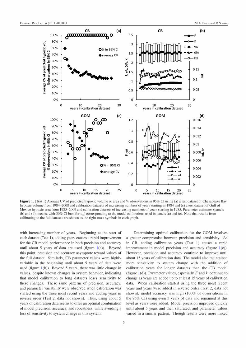
Environ Res Lett 6 (2011) 015001 M A Evans and D Scavia
Mississippi RiverGulf of Mexico Watershed Nutrient TaskForce 2008 Gulf Hypoxia Action Plan 2008 for ReducingMitigating and Controlling Hypoxia in the Northern Gulf ofMexico and Improving Water Quality in the Mississippi RiverBasin (Washington DC USEPA Office of Wetlands Oceansand Watersheds) (Action Plan available at wwwepagovowow keepmsbasinactionplanhtm)
Pena M A Katsev S Oguz T and Gilbert D 2010 Modeling dissolvedoxygen dynamics and hypoxia Biogeosciences 7 933ndash57
Penta B et al 2009 Using coupled models to study the effects of riverdischarge on biogeochemical cycling and hypoxia in thenorthern Gulf of Mexico OCEANS 2009 MTSIEEEBiloxi-Marine Technology for our Future Global and LocalChallenges (New York NY IEEE) pp 1ndash7 (available fromhttpieeexploreieeeorgstampstampjsptp=amparnumber=5422347ampisnumber=5422059)
Rabalais N N 2009 personal communicationRabalais N N 2006 Oxygen depletion in the Gulf of Mexico adjacent
to the Mississippi river Gayana (Concepc) 70 73ndash8Rabalais N N Atilla N Normandeau C and Turner R E 2004
Ecosystem history of Mississippi river-influenced continentalshelf revealed through preserved phytoplankton pigments MarPollut Bull 49 537ndash47
Rabalais N N and Turner R E 2001 Coastal Hypoxia Consequencesfor Living Resources and Ecosystems (Washington DCAmerican Geophysical Union)
Rabalais N N Turner R E Dortch Q Justic D Bierman V J andWiseman W J 2002a Nutrient-enhanced productivity in thenorthern Gulf of Mexico past present and futureHydrobiologia 475 39ndash63
Rabalais N N Turner R E and Scavia D 2002b Beyond science intopolicy Gulf of Mexico hypoxia and the Mississippi riverBioscience 52 129ndash42
Rabalais N N Turner R E Sen Gupta B K Boesch D FChapman P and Murrell M C 2007 Hypoxia in the northernGulf of Mexico does the science support the plan to reducemitigate and control hypoxia Estuaries Coasts 30 753ndash72
Rabalais N N Turner R E and Wiseman W J 2002c Gulf of Mexicohypoxia aka lsquoThe dead zonersquo Annu Rev Ecol Syst 33 235ndash63
Rabalais N N Turner R E Wiseman W J and Dortch Q 1998Consequences of the 1993 Mississippi river flood in the Gulf ofMexico Regul Rivers-Res Manag 14 161ndash77
Rabalais N N Wiseman W J and Turner R E 1994 Comparison ofcontinuous records of near-bottom dissolved-oxygen from thehypoxia zone along the Louisiana coast Estuaries 17 850ndash61
Renaud M L 1986 Hypoxia in Louisiana coastal waters during1983mdashimplications for fisheries Fishery Bull 84 19ndash26(available at httpfishbullnoaagov841renaudpdf)
Scavia D and Donnelly K A 2007 Reassessing hypoxia forecasts forthe Gulf of Mexico Environ Sci Technol 41 8111ndash7
Scavia D Justic D and Bierman V J 2004 Reducing hypoxia in theGulf of Mexico advice from three models Estuaries 27 419ndash25
Scavia D Kelly E L A and Hagy J D 2006 A simple model forforecasting the effects of nitrogen loads on Chesapeake Bayhypoxia Estuaries Coasts 29 674ndash84
Scavia D Rabalais N N Turner R E Justic D and Wiseman W J 2003Predicting the response of Gulf of Mexico hypoxia to variationsin Mississippi river nitrogen load Limnol Oceanogr 48 951ndash6
Scheffer M and van Nes E H 2007 Shallow lakes theory revisitedvarious alternative regimes driven by climate nutrients depthand lake size Hydrobiologia 584 455ndash66
Scully M E 2010 The importance of climate variability towind-driven modulation of hypoxia in Chesapeake Bay J PhysOceanogr 40 1435ndash40
Stow C A and Scavia D 2009 Modeling hypoxia in the ChesapeakeBay ensemble estimation using a Bayesian hierarchical modelJ Mar Syst 76 244ndash50
Turner R E Rabalais N N and Justic D 2006 Predicting summerhypoxia in the northern Gulf of Mexico riverine N P and Siloading Mar Pollut Bull 52 139ndash48
Turner R E Rabalais N N and Justic D 2008 Gulf of Mexico hypoxiaalternate states and a legacy Environ Sci Technol 42 2323ndash7
Turner R E Rabalais N N Swenson E M Kasprzak M andRomaire T 2005 Summer hypoxia in the northern Gulf ofMexico and its prediction from 1978 to 1995 Mar Environ Res59 65ndash77
USGS 2007 Chesapeake Bay River Input Monitoring ProgramLoads (available online at httpvawaterusgsgovchesbayRIMPloadshtml) (accessed 10 May 2010)
USGS 2009 Streamflow and Nutrient Delivery to the Gulf of Mexico(available online at httptoxicsusgsgovhypoxiamississippiflux estsdeliveryindexhtml) (accessed 14 June 2010)
USGS 2010 Streamflow and Nutrient Delivery to the Gulf of Mexicofor October 2009 to May 2010 (Preliminary) (available onlineat httptoxicsusgsgovhypoxiamississippioct junindexhtml) (accessed 20 June 2010)
Walker N D and Rabalais N N 2006 Relationships among satellitechlorophyll a river inputs and hypoxia on the Louisianacontinental shelf Gulf of Mexico Estuaries Coasts 29 1081ndash93
Wang L X and Justic D 2009 A modeling study of the physicalprocesses affecting the development of seasonal hypoxia overthe inner LouisianandashTexas shelf circulation and stratificationCont Shelf Res 29 1464ndash76
Zhang J et al 2010 Natural and human-induced hypoxia andconsequences for coastal areas synthesis and futuredevelopment Biogeosciences 7 1443ndash67
11
- 1 Introduction
- 2 Methods
-
- 21 Models
- 22 Data sources
- 23 Hindcast and forecast tests
- 24 Response curves
-
- 3 Results
-
- 31 Full dataset calibration
- 32 Effect of number of years in the calibration
- 33 Moving window calibrations case 1---averaging vi
- 34 Moving window calibrations case 2---constant v
-
- 4 Discussion
-
- 41 Forecasts
-
- 5 Conclusions
- Acknowledgments
- References
-