AQUATIC BIOLOGYAquat Biol

Vol. 20: 77–90, 2014doi: 10.3354/ab00541

Published January 13

INTRODUCTION

Our understanding of salmonid behavior and eco -logy during ocean residence is limited relative to thatof other life-history stages (Hartt & Dell 1986, Quinn2005). However, for many individuals, ocean resi-dence represents the longest stage of the life history.For example, Chinook salmon Oncorhynchus tshawyt -scha typically spend the first year in freshwater andthen 1 to 5 yr in the Pacific Ocean before returning tospawn. Yearling Chinook salmon from the ColumbiaRiver enter the ocean and quickly migrate north(Peterson et al. 2010). Although general migrationpatterns are known (Weitkamp 2010, Tucker et al.2011) and environmental correlates have been pro-posed (Bi et al. 2007, Burla et al. 2010a, Peterson etal. 2010, Burke et al. 2013), a comprehensive under-

standing of the early ocean ecology and migrationbehavior of these juvenile salmon is missing.

One of the more difficult aspects of studying juvenile salmon ocean ecology is understanding thebehavioral responses of these fish to external stimuli.For example, what cues do salmon use as aids duringmigration? Do fish make behavioral decisions basedon local environmental conditions, so as to maximizetheir short-term growth rate? This would be a logicalobjective, given that mortality during early ocean re -sidence is often size-dependent (Healey 1982, Goodet al. 2001, Moss et al. 2005, Cross et al. 2009). Orhave salmon evolved a northward migration strategythat relies on large-scale navigational aids, as hasbeen shown for other animals (Wiltschko & Wiltschko1995, Papi 2006)? Although Alaskan coastal waterstend to be more productive than those off Oregon

© The authors 2014. Open Access under Creative Commons byAttribution Licence. Use, distribution and reproduction are un -restricted. Authors and original publication must be credited.

Publisher: Inter-Research · www.int-res.com

*Corresponding author: brian.burke@noaa.gov

Evidence for multiple navigational sensory capabilities of Chinook salmon

Brian J. Burke1,2,*, James J. Anderson2, António M. Baptista3

1Fish Ecology Division, Northwest Fisheries Science Center, National Marine Fisheries Service, National Oceanic and Atmospheric Administration, Seattle, Washington 98112, USA

2School of Aquatic and Fishery Sciences, University of Washington, Seattle, Washington 98195, USA3Center for Coastal Margin Observation & Prediction, Oregon Health & Science University, Beaverton, Oregon 97006, USA

ABSTRACT: To study the complex coastal migrations patterns exhibited by juvenile ColumbiaRiver Chinook salmon as they enter and move through the marine environment, we created anindividual-based model in a coupled Eulerian-Lagrangian framework. We modeled 5 distinctmigration strategies and compared the resulting spatial distributions to catch data collected dur-ing May and June in 3 years. Two strategies produced fish distributions similar to those observedin May, but only one also produced the observed June distributions. In both strategies, salmon dis-tinguish north from south (i.e. they have a compass sense), and they control their position relativeto particular landmarks, such as the river mouth. With these 2 abilities, we posit that salmon followspatially explicit behavior rules that prevent entrapment in strong southward currents and advec-tion offshore. Additionally, the consistent spatio-temporal distributions observed among yearssuggest that salmon use a clock sense to adjust their swim speed, within and among years, inresponse to progress along their migration.

KEY WORDS: Chinook salmon · Oncorhynchus tshawytscha · Migration · Navigation · Individual-based model · Behavior

OPENPEN ACCESSCCESS

Aquat Biol 20: 77–90, 2014

and Washington, fish leaving the Columbia Riverhave no cognitive knowledge of this fact.

The ability of salmon to consistently migrate to relatively specific locations, both as smolts and adults,has driven a large body of research. Salmon appearto use multiple cues, depending on the cue availabil-ity and the stage of migration (Dittman & Quinn 1996,Quinn 2005). Groot (1965) first demonstrated thatsalmon use celestial cues for orientation but switch to‘some as yet unknown set of reference cues’ as cloudcover increases. A series of experiments on sockeyesalmon fry and smolts (Quinn 1980, Quinn et al. 1981,Quinn & Brannon 1982) then revealed that, in theabsence of alternative information, salmon orientedusing the Earth’s magnetic field; an ability found in awide range of animals (Wiltschko & Wiltschko 1995,Papi 2006, Lohmann et al. 2007). Indeed, recent workhas identified magnetite-based magnetoreceptors inboth salmon and trout (Kirschvink et al. 1985, Walkeret al. 1988, 1997) as well as the use of the magneticfield in adult salmon during their return migration(Bracis & Anderson 2012, Putman et al. 2013). Yet, asdiscussed by Friedland et al. (2001), our understand-ing of the relative role of these reference systems isstill limited, particularly in the marine environment.

Willis (2011) distinguishes 2 general processes in -volved in migration: navigation is movement towarda goal outside of the sensory environment of an ani-mal, and orientation is a directional response to localconditions (it should be noted that multiple defini-tions exist in the literature). By this definition, navi-gation requires a compass sense, while orientation mayonly require knowledge of ambient environmentalconditions (e.g. an animal could orient relative to atemperature or salinity gradient). Burke et al. (2013)found that the response to (unspecified) large-scalevariables, such as the sun or Earth’s magnetic field,was stronger than the response to local environmen-tal cues, which suggests that salmon primarily usenavigation in their migrations. However, orientationto local conditions is also suggested by the high cor-relation between yearling Chinook salmon catchesand local environmental conditions (Bi et al. 2007,Burla et al. 2010a, Yu et al. 2012, Burke et al. 2013).

To explore in more detail the importance of globalnavigation and local orientation in salmon migrationbehavior, we simulated fish movement through a vir-tual environment using an individual-based model(IBM) in a coupled Eulerian-Lagrangian framework(similar models were reviewed by North et al. 2009,Kishi et al. 2011, Willis 2011, Byron & Burke in press).An individual fish makes thousands of behavioraldecisions every day based on its environment, condi-

tion, and genetic makeup. We simulated these deci-sions and the resulting movement of individual fishusing prescribed behaviors in response to a dynamicphysical environment. By integrating specific behav-ioral responses over a time series of environmentalconditions experienced by the fish, we identifiedwhich behaviors produced realistic fish trajectoriesand final locations.

Using this tool, we tested a suite of plausible be -haviors to characterize the effect of various orien -tation and navigation cues on the spatio-temporaldistribution of juvenile salmon in the marine environ-ment. Because of the complexity of migratory behav-ior and cues that direct migration, our aim was toeliminate some behaviors and cues as infeasible whileidentifying others that may be significant. In thisway, our goal was to reduce the set of possible factorsthat need to be considered when studying salmonidmigration and studying how existing migratory pat-terns may respond to local and global changes in themarine environment.

MATERIALS AND METHODS

A number of movement-modeling frameworks (e.g.reaction-diffusion equations) are inadequate to rep-resent the complex coastal currents and concomitantocean migration behaviors employed by salmon.We therefore used a combination of Eulerian andLagrangian frameworks to simulate fish movementthrough a virtual environment (Willis 2011). Specifi-cally, we used output from a Eulerian hydrodynamicmodel as the virtual environment (rather than dy -namically simulating fish movement within the hydro -dynamic model) and created a Lagrangian IBM thatgenerated individual fish movements and behaviorswithin the environment.

After modeling fish with individualized responsesto the environment, we summarized the set of modeled individuals to determine population-level spatio-temporal distributions. Simulations were imple-mented in the Python language (PSF 2013). Below,we describe the salmon data used in the simulations,the hydrodynamic model that generated the virtualenvironment, the details of the IBM, and, finally, howwe analyzed the results.

Salmon catch data

Several distinct stocks of Chinook salmon from theColumbia River Basin, western USA, migrate as year-

78

Burke et al.: Chinook salmon sensory capabilities

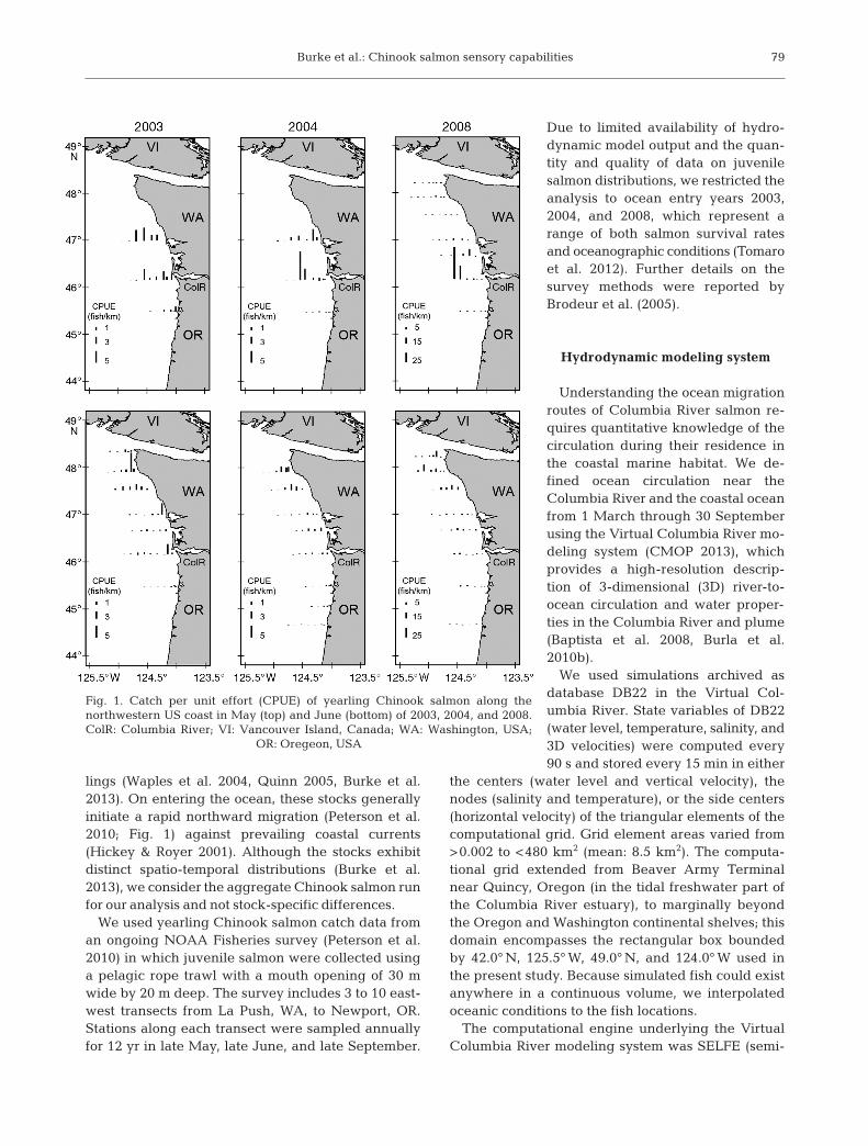
lings (Waples et al. 2004, Quinn 2005, Burke et al.2013). On entering the ocean, these stocks generallyinitiate a rapid northward migration (Peterson et al.2010; Fig. 1) against prevailing coastal currents(Hickey & Royer 2001). Although the stocks exhibitdistinct spatio-temporal distributions (Burke et al.2013), we consider the aggregate Chinook salmon runfor our analysis and not stock-specific differences.

We used yearling Chinook salmon catch data froman ongoing NOAA Fisheries survey (Peterson et al.2010) in which juvenile salmon were collected usinga pelagic rope trawl with a mouth opening of 30 mwide by 20 m deep. The survey includes 3 to 10 east-west transects from La Push, WA, to Newport, OR.Stations along each transect were sampled annuallyfor 12 yr in late May, late June, and late September.

Due to limited availability of hydro-dynamic model output and the quan-tity and quality of data on juvenilesalmon distributions, we restricted theanalysis to ocean entry years 2003,2004, and 2008, which represent arange of both salmon survival ratesand oceanographic conditions (Tomaroet al. 2012). Further details on the survey methods were reported byBrodeur et al. (2005).

Hydrodynamic modeling system

Understanding the ocean migrationroutes of Columbia River salmon re -quires quantitative knowledge of thecirculation during their residence inthe coastal marine habitat. We de-fined ocean circulation near theColumbia River and the coastal oceanfrom 1 March through 30 Septemberusing the Virtual Columbia River mo -deling system (CMOP 2013), whichprovides a high-resolution descrip-tion of 3-dimensional (3D) river-to-ocean circulation and water proper-ties in the Columbia River and plume(Baptista et al. 2008, Burla et al.2010b).

We used simulations archived asdatabase DB22 in the Virtual Col -umbia River. State variables of DB22(water level, temperature, salinity, and3D velocities) were computed every90 s and stored every 15 min in either

the centers (water level and vertical velocity), thenodes (salinity and temperature), or the side centers(horizontal velocity) of the triangular elements of thecomputational grid. Grid element areas varied from>0.002 to <480 km2 (mean: 8.5 km2). The computa-tional grid extended from Beaver Army Terminalnear Quincy, Oregon (in the tidal freshwater part ofthe Columbia River estuary), to marginally beyondthe Oregon and Washington continental shelves; thisdomain encompasses the rectangular box boundedby 42.0° N, 125.5° W, 49.0° N, and 124.0° W used inthe present study. Because simulated fish could existanywhere in a continuous volume, we interpolatedoceanic conditions to the fish locations.

The computational engine underlying the VirtualColumbia River modeling system was SELFE (semi-

79

Fig. 1. Catch per unit effort (CPUE) of yearling Chinook salmon along the northwestern US coast in May (top) and June (bottom) of 2003, 2004, and 2008.ColR: Columbia River; VI: Vancouver Island, Canada; WA: Washington, USA;

OR: Oregeon, USA

Aquat Biol 20: 77–90, 2014

implicit Eularian-Lagrangian finite-element), a baro-clinic circulation model based on the solution of 3Dshallow water equations (Zhang & Baptista 2008).These consisted of a continuity equation, conserva-tion equations for momentum, salinity, and heat, andan equation of state, which used a finite-elementmethod applied on an unstructured, 3-node tri -angular grid. The skill of these simulations had beenpreviously assessed through quantitative comparisonagainst observations of water level, salinity, and temperature from the Science and Technology Uni-versity Research Network (SATURN) collaboratory(Baptista et al. 2005, Burla et al. 2010b).

Individual-based model

We describe the IBM using the overview, designconcepts, and details (ODD) protocol of Grimm et al.(2006, 2010). The overview portion includes the pur-pose of the model, the state variables and scalesused, and an overview of the processes and schedul-ing. We then describe the details of initialization,model input, and several submodels.

Overview

Purpose. After salmon leave the Columbia River,there is little known about the routes taken duringtheir initial migration, and even less is known aboutthe behaviors they employ during this stage. Thismodel is intended to (1) distinguish between feasibleand unrealistic behaviors, given the constraints of

coastal currents, fish size, and post-smolt migrationtiming, and (2) evaluate various migration behaviorsby comparing simulated spatio-temporal distributionsto observed distributions.

State variables and scales. Environmental statevariables included temperature, salinity, 3D flow,and water depth. For some simulations, distancefrom shore and chlorophyll a concentration were alsoexplicitly used as a driving variable.

Fish were assigned an ocean entry date and an ini-tial 3D location, which was updated at every 15 mintime step of the simulation. Fish size was alsoupdated at every time step using a standard bioener-getics model with parameters for Chinook salmon(Hewett & Johnson 1992). Consumption was mod-eled using a proportion of maximum daily consump-tion, or P-value (a size- and temperature-dependentvariable), and each fish kept its randomly assignedP-value for the duration of the simulation. Similarly, ifa simulation employed active swimming (Table 1),assigned swim speeds (body lengths [BL] per second)were maintained for the duration of the simulation,such that speed relative to the water increased as fishgrew.

Process and scheduling. Each simulation started at00:15 h on 1 April and ran through midnight on 1July. During each time step, fish first grew accordingto the bioenergetics model, local temperature, andassigned P-value. Fish then moved to a new location,where they stayed until the next time step. Thegrowth and movement of each fish was independentof that of other fish as there was no direct or indirectinteraction among individuals. While mortality is highduring the early ocean stage (Pearcy 1992, Beamish

80

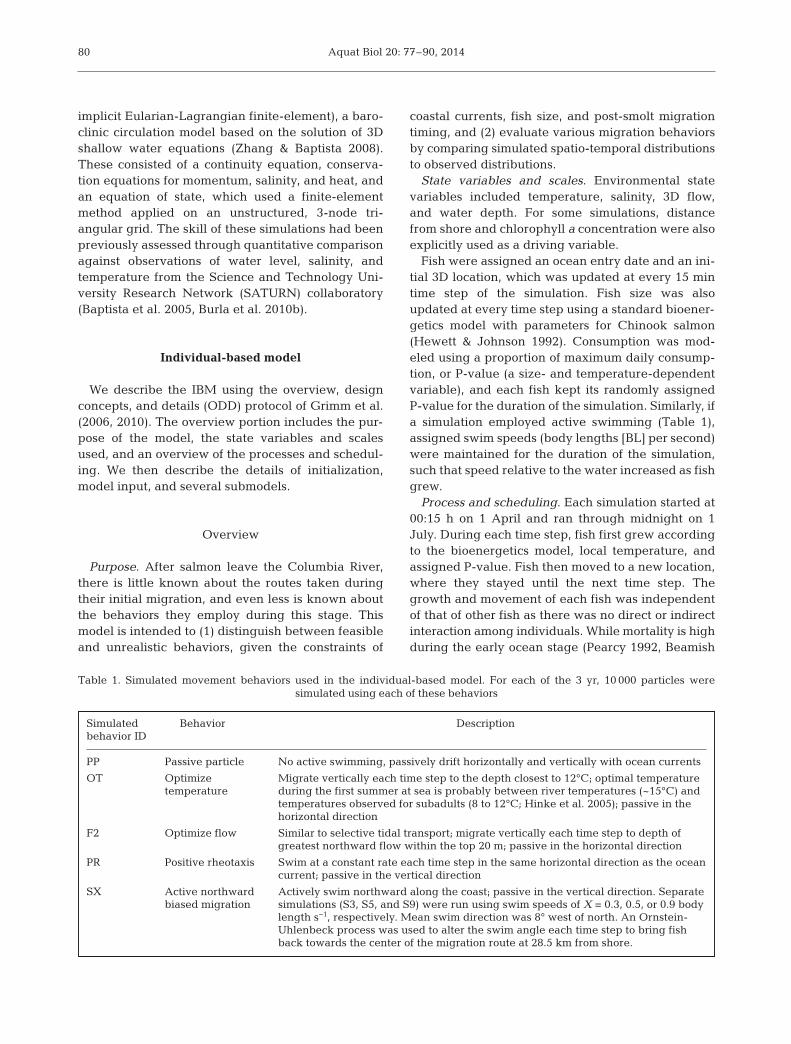
Simulated Behavior Descriptionbehavior ID

PP Passive particle No active swimming, passively drift horizontally and vertically with ocean currents

OT Optimize Migrate vertically each time step to the depth closest to 12°C; optimal temperature temperature during the first summer at sea is probably between river temperatures (~15°C) and temperatures observed for subadults (8 to 12°C; Hinke et al. 2005); passive in the

horizontal direction

F2 Optimize flow Similar to selective tidal transport; migrate vertically each time step to depth ofgreatest northward flow within the top 20 m; passive in the horizontal direction

PR Positive rheotaxis Swim at a constant rate each time step in the same horizontal direction as the oceancurrent; passive in the vertical direction

SX Active northward Actively swim northward along the coast; passive in the vertical direction. Separate biased migration simulations (S3, S5, and S9) were run using swim speeds of X = 0.3, 0.5, or 0.9 body

length s−1, respectively. Mean swim direction was 8° west of north. An Ornstein-Uhlenbeck process was used to alter the swim angle each time step to bring fishback towards the center of the migration route at 28.5 km from shore.

Table 1. Simulated movement behaviors used in the individual-based model. For each of the 3 yr, 10 000 particles were simulated using each of these behaviors

Burke et al.: Chinook salmon sensory capabilities

& Mahnken 2001), we had insufficient information topartition mortality spatially or temporally. Therefore,all simulated fish were considered survivors of thefirst 3 mo in the marine environment.

Design concepts

Basic principles. Optimal swim speed for both traveland foraging is size-dependent (Ware 1978), as aremany ecological processes acting on individuals(Arendt 1997, Sogard 1997). We included a bioener-getics model to allow individual growth throughoutthe simulation, such that all size-dependent processesin the model (e.g. growth and swimming speed)affected fish appropriately.

As this model describes the migration of animalsthrough a dynamic environment, we tested behaviorsrelated to both movement theory and habitat selec-tion. Among the behavioral rules, we included pas-sive drift, diffusion, and directed migration. In otherrules, we explicitly tested habitat selection usingmultiple temperature-based behaviors as well as somebehaviors involving distance from shore (Table 1).

Adaptation. Columbia River yearling Chinook sal -mon are consistently captured in a narrow east-westband (mean distance from shore = 28.5 km, SD =7.6 km) along the Washington coast (Peterson et al.2010), but our efforts to mechanistically model sucha narrow migration corridor were unsuccessful. Asthe northward migration was our primary focus, we simplified the model by imposing an attraction to aspecific east-west location. For simulations involvingbehavior SX (behaviors are described below and inTable 1), we used an Ornstein−Uhlenbeck process toadjust the swim angle. In this framework, the greaterthe distance between a fish and the line of attraction,the more its swim angle was shifted back toward theline. This resulted in swim angles of ~320° for fishon the shoreline and ~45° for fish 80 km offshore.Although the mechanism by which fish maintaintheir east-west location is unknown, inclusion of thisline of attraction was necessary to keep simulatedfish from migrating into land or far offshore. Meandistance from shore for yearling Chinook salmonsampled over 12 yr (Peterson et al. 2010) was 28.5 km,and we used this as the line of attraction.

Sensing and prediction. Ambient conditions suchas temperature and flow were used to determine fishbehavior. Simulated fish had no explicit knowledgeof environmental conditions at any spatial coordi-nates other than their immediate location, with theexception of vertical structure used to optimize verti-

cal temperature (OT) and flow (F2). For these behav-iors, fish selected specific attributes from within thewater column. The thermocline was usually shallow(~10 m), and it is certainly feasible that fish regularlymake short vertical movements within a 15 min timestep to determine vertical temperature or flow profiles.

On a larger temporal and spatial scale, we postu-lated that fish are inherently inclined to migratenorth, which implies a genetically selected pro pensityto migrate to regions that have historically allowedhigher growth and/or survival. For these simulations,we made 2 assumptions regarding spatial infor -mation: (1) fish had a compass sense and thereforeknew what direction was north (Quinn & Groot 1983,Quinn 1991), and (2) fish knew their distance fromshore. For the latter assumption, we do not know thenature of the cue, but it is likely to involve one ormore oceanographic features.

Stochasticity. We started all simulations with thesame random number seed in the Python language,so that all randomly drawn variables (initial length,ocean entry date, P-value, and initial depth) wereidentical among simulations. Therefore, each simula-tion (within a year) tested the same initial set of 10 000randomly drawn fish with the only difference amongsimulations being fish behavior (see ‘Initialization’).

Observation. We stored all initial data (length,location, P-value, and swim speed) to files. Every12 h of simulated time, we recorded the location andlength of all fish. All data were imported into R soft-ware for analysis (R Development Core Team 2011).

Details

Initialization. At the start of a simulation, we gener-ated 10 000 virtual fish and assigned initial valuesfor all state variables. Fish sizes (μ = 155 mm, SD =15 mm) and ocean entry dates (μ = 15 May, SD =10 d) were drawn randomly from normal distributions(Table 2), roughly matching empirical data collectedin the Columbia River estuary (Weitkamp et al. 2012).Fish initiated migrations just inside the Columbia Rivermouth (latitude 46.2482° N, longitude −124.0759° W)at randomly (uniformly) assigned depths within thetop 10 m. The proportion of the maximum daily con-sumption rate (P-value) of each fish was drawn froma log-normal distribution (μ = log(0.5), SD = 0.5).

Input. All input data were obtained from the hydro-dynamic modeling system described above (Zhang& Baptista 2008) except chlorophyll a, which wasobtained from a satellite via the NOAA CoastWatchProgram (PFEL 2013).

81

Aquat Biol 20: 77–90, 2014

Growth submodel. We modeled fish growth usinga standard bioenergetics model parameterized forChinook salmon (Hewett & Johnson 1992). In each15 min time step, fish first instantaneously grew andthen moved. As most bioenergetics models are para-meterized for a 24 h time step, we divided all rateconstants (e.g. consumption) by 96 to match our 15 mintime step. To maintain a widening gap between thelargest and smallest fish throughout the simulation,maximum daily consumption (P-values) did not changewithin a simulation. This also reduced the stochastic-ity of the model and allowed comparisons of indi -vidual fish among simulations (results not shown),where the only difference between the fish was theassigned behavior (Table 1).

Movement submodel. We defined 5 distinct be -havioral rules (Table 1). Swimming through water isenergetically expensive, and our set of migrationstrategies was chosen to determine whether simpleand efficient behaviors were sufficient to simulatethe observed fish distributions or whether more com-plex and energetically costly behaviors were required.The null behavior, passive particle (PP), assumed fishwere passive in 3 dimensions (Willis & Hobday 2007,Brochier et al. 2008) and served as a particle tracer ofocean currents.

For the optimum temperature behavior (OT), fishmaintained the optimum temperature for growth,which we assumed to be 12°C based on results fromHinke et al. (2005), via vertical movement during eachtime step. Horizontal movement for this behaviorwas passive. Similarly, there was no active horizontalmovement for the optimizing flow behavior (F2), inwhich fish selectively adjusted their depth withinthe top 20 m to maximize northward movement (seeBurke et al. 2013 for justification of the 20 m cutoff).Essentially, fish move vertically into slow water whenflows are southerly and into fast water when flows arenortherly, thus maximizing net northward displace-ment without active horizontal swimming (Lacroix &McCurdy 1996). Using local currents to aid movement

has been shown for many migrat-ing species, including tuna, moths(Alerstam et al. 2011), and At-lantic salmon Salmo salar (Thor -stad et al. 2012). To employ theselection of northward currentsin this behavior, animals requireda compass sense.

We simulated 2 behaviors thatinvolved active horizontal move-ment. The positive rheotaxis (PR)behavior was similar to that used

in other coupled oceanographic and IBM, which haveshown that swimming with or against currents couldbe a successful migration strategy (Booker et al. 2008,Mork et al. 2012). During the positive rheotaxis simu-lations, fish maintained a swim speed of 0.5 BL s−1 di-rectly into the prevailing current. Although we reportresults only for positive rheotaxis, we also ran simula-tions using negative rheotaxis. However, ocean cur-rents in this region are predominantly southern in thespringtime (Hickey & Royer 2001), and therefore, neg-ative rheotaxis was obviously not a viable strategy.

Finally, we simulated active northward swimming(SX), independent of local environmental conditions.Three swim speeds were individually simulated (0.3,0.5, and 0.9 BL s−1) at a mean angle of 8° west of north(approximately along the coastline), adjusted eachtime step according the Ornstein-Uhlenbeck modeldescribed above. Like the behavior to optimize flow,the active northward migration behavior requiredthat fish have a compass sense.

Analysis

Final locations of simulated fish were compared tothe spatial distribution of yearling Chinook salmoncaught during the NOAA Fisheries surveys (Fig. 1;Brodeur et al. 2005). To select feasible behaviors, weused a combination of visual comparisons and simplesummary metrics (e.g. mean final latitude). Our goalwas to provide relative support for or against migra-tion behaviors rather than to prove that salmon useany particular behavior. Moreover, the simulateddata (a point process) and the observed data (densityestimates at discrete locations) were not directlycomparable quantitatively (most spatial statistics re -quire either a point process or a density estimate[Bivand et al. 2013]; we are not aware of statisticalmethods to compare the 2 types directly).

We summarized simulated data from 26 May and26 June, corresponding to the middle dates of re -

82

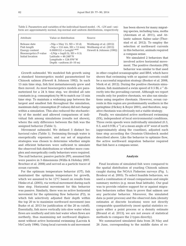
Attribute Value or distribution Source

Release date ~N(μ = May 15, SD = 10 d) Weitkamp et al. (2012)Fish length ~N(μ = 155 mm, SD = 15 mm) Weitkamp et al. (2012)Energy content 0.0000152 × Length2.9648 Hewett & Johnson (1992)Bioenergetics P-value ~LN(μ = log(0.5), SD = 0.5)Initial location Latitude = 46.248°N

Longitude = 124.076°WDepth ~uniform (0−10 m)

Table 2. Parameters and variables of the individual-based model. ~N, ~LN and ~uni-form are approximately normal, log-normal and uniform distributions, respectively

Burke et al.: Chinook salmon sensory capabilities

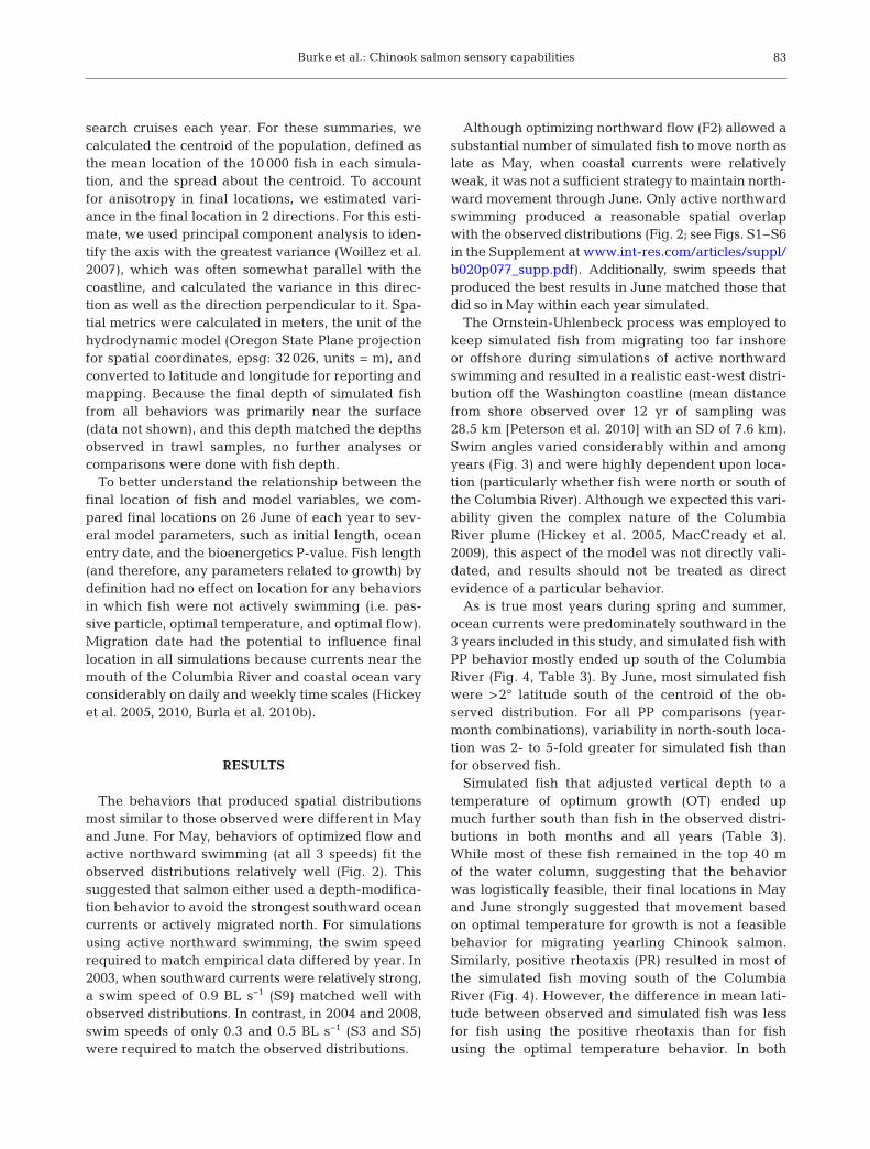
search cruises each year. For these summaries, wecalculated the centroid of the population, defined asthe mean location of the 10 000 fish in each simula-tion, and the spread about the centroid. To accountfor anisotropy in final locations, we estimated vari-ance in the final location in 2 directions. For this esti-mate, we used principal component analysis to iden-tify the axis with the greatest variance (Woillez et al.2007), which was often somewhat parallel with thecoastline, and calculated the variance in this direc-tion as well as the direction perpendicular to it. Spa-tial metrics were calculated in meters, the unit of thehydrodynamic model (Oregon State Plane projectionfor spatial coordinates, epsg: 32 026, units = m), andconverted to latitude and longitude for reporting andmapping. Because the final depth of simulated fishfrom all behaviors was primarily near the surface(data not shown), and this depth matched the depthsobserved in trawl samples, no further analyses orcomparisons were done with fish depth.

To better understand the relationship between thefinal location of fish and model variables, we com-pared final locations on 26 June of each year to sev-eral model parameters, such as initial length, oceanentry date, and the bioenergetics P-value. Fish length(and therefore, any parameters related to growth) bydefinition had no effect on location for any behaviorsin which fish were not actively swimming (i.e. pas-sive particle, optimal temperature, and optimal flow).Migration date had the potential to influence finallocation in all simulations because currents near themouth of the Columbia River and coastal ocean varyconsiderably on daily and weekly time scales (Hickeyet al. 2005, 2010, Burla et al. 2010b).

RESULTS

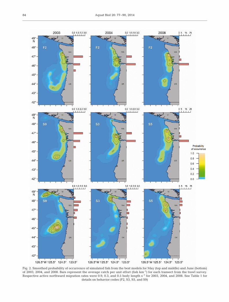
The behaviors that produced spatial distributionsmost similar to those observed were different in Mayand June. For May, behaviors of optimized flow andactive northward swimming (at all 3 speeds) fit theobserved distributions relatively well (Fig. 2). Thissuggested that salmon either used a depth-modifica-tion behavior to avoid the strongest southward oceancurrents or actively migrated north. For simulationsusing active northward swimming, the swim speedrequired to match empirical data differed by year. In2003, when southward currents were relatively strong,a swim speed of 0.9 BL s−1 (S9) matched well withobserved distributions. In contrast, in 2004 and 2008,swim speeds of only 0.3 and 0.5 BL s−1 (S3 and S5)were required to match the observed distributions.

Although optimizing northward flow (F2) allowed asubstantial number of simulated fish to move north aslate as May, when coastal currents were relativelyweak, it was not a sufficient strategy to maintain north -ward movement through June. Only active north wardswimming produced a reasonable spatial overlapwith the observed distributions (Fig. 2; see Figs. S1–S6in the Supplement at www.int-res.com/ articles/suppl/b020 p077_ supp.pdf). Additionally, swim speeds thatproduced the best results in June matched those thatdid so in May within each year simulated.

The Ornstein-Uhlenbeck process was employed tokeep simulated fish from migrating too far inshoreor offshore during simulations of active northwardswimming and resulted in a realistic east-west distri-bution off the Washington coastline (mean distancefrom shore observed over 12 yr of sampling was28.5 km [Peterson et al. 2010] with an SD of 7.6 km).Swim angles varied considerably within and amongyears (Fig. 3) and were highly dependent upon loca-tion (particularly whether fish were north or south ofthe Columbia River). Although we expected this vari-ability given the complex nature of the ColumbiaRiver plume (Hickey et al. 2005, MacCready et al.2009), this aspect of the model was not directly vali-dated, and results should not be treated as direct evidence of a particular behavior.

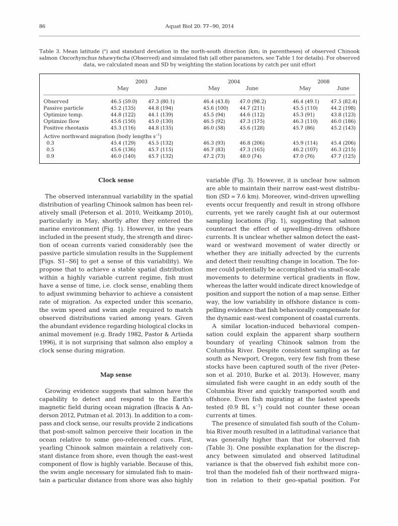
As is true most years during spring and summer,ocean currents were predominately southward in the3 years included in this study, and simulated fish withPP behavior mostly ended up south of the ColumbiaRiver (Fig. 4, Table 3). By June, most simulated fishwere >2° latitude south of the centroid of the ob -served distribution. For all PP comparisons (year-month combinations), variability in north-south loca-tion was 2- to 5-fold greater for simulated fish thanfor observed fish.

Simulated fish that adjusted vertical depth to atemperature of optimum growth (OT) ended upmuch further south than fish in the observed distri-butions in both months and all years (Table 3).While most of these fish remained in the top 40 mof the water column, suggesting that the behaviorwas logistically feasible, their final locations in Mayand June strongly suggested that movement basedon optimal temperature for growth is not a feasiblebehavior for mi grating yearling Chinook salmon.Similarly, positive rheotaxis (PR) resulted in most ofthe simulated fish moving south of the ColumbiaRiver (Fig. 4). However, the difference in mean lati-tude between observed and simulated fish was lessfor fish using the positive rheotaxis than for fishusing the optimal temperature behavior. In both

83

Aquat Biol 20: 77–90, 201484

Fig. 2. Smoothed probability of occurrence of simulated fish from the best models for May (top and middle) and June (bottom)of 2003, 2004, and 2008. Bars represent the average catch per unit effort (fish km–1) for each transect from the trawl survey. Respective active northward migration rates were 0.9, 0.3, and 0.5 body length s−1 for 2003, 2004, and 2008. See Table 1 for

details on behavior codes (F2, S3, S5, and S9)

Burke et al.: Chinook salmon sensory capabilities

cases, we did not see a large effect of fish size onmovement and distribution.

In all simulations, including those that bestmatched observed spatial patterns, some fish werepushed south of the Columbia River just after oceanentrance. Although the proportion of fish pushedsouth varied by year and behavior (Fig. 4), very fewfish were able to counter the strong southward flows,upwelling-driven offshore currents, and eddies thatcarried them offshore. In some cases, these advected

fish had a large influence on summary metrics, suchas mean final location (Table 3, see Figs. S1–S6 inthe Supplement). Interestingly, the subset of fishadvected south was not influenced to a large extentby length, growth, or ocean entry date (see Fig. S7 inthe Supplement).

DISCUSSION

The simulations suggest that Columbia River year-ling Chinook salmon use at least 2 sensory modalitiesduring migration: a compass sense and a clock sense.In addition, there is some tentative evidence that fishuse a map sense, although other modalities may beinvolved. Evidence for each modality arises from dif-ferent aspects of the simulations, as described below.

Compass sense

For most of the behaviors modeled, the predomi-nantly southward flowing coastal currents preventedsimulated fish from migrating north. In fact, most behaviors resulted in fish moving quite far southand offshore of the Oregon coast. Counter to ourinitial ex pectations, positive rheotaxis alone was in-sufficient to produce northward migration since thecoastal currents were too complex to produce a con-sist cue for northward movement. The only behaviorsthat produced the observed northern distributions offish were optimization of northward flows via verti-cal migration (F2) and/or active northward swimming(SX). Since both of these behaviors require that fishsense the direction north, we concluded that salmonuse a compass sense during their marine migration.

85

Fig. 3. Frequency of turn angles by fish throughout the en-tire simulation. Results are from simulations using the activenorthward migration behavior and the best swim speed foreach year: 0.9 body lengths (BL) s−1 in 2003, 0.3 BL s−1 in2004, and 0.5 BL s−1 in 2008. The large proportion of fishswimming at 90° is due to fish south of the Columbia Riverthat were advected offshore and were trying to compensate

Fig. 4. Proportion of simulated fish south of latitude 46° N according to behavior for May and June of 2003, 2004, and 2008. See Table 1 for behavior codes

Aquat Biol 20: 77–90, 2014

Clock sense

The observed interannual variability in the spatialdistribution of yearling Chinook salmon has been rel-atively small (Peterson et al. 2010, Weitkamp 2010),particularly in May, shortly after they entered themarine environment (Fig. 1). However, in the yearsincluded in the present study, the strength and direc-tion of ocean currents varied considerably (see thepassive particle simulation results in the Supplement[Figs. S1–S6] to get a sense of this variability). Wepropose that to achieve a stable spatial distributionwithin a highly variable current regime, fish musthave a sense of time, i.e. clock sense¸ enabling themto adjust swimming behavior to achieve a consistentrate of mi gration. As expected under this scenario,the swim speed and swim angle required to matchobserved distributions varied among years. Giventhe abundant evidence regarding biological clocks inanimal movement (e.g. Brady 1982, Pastor & Artieda1996), it is not surprising that salmon also employ aclock sense during migration.

Map sense

Growing evidence suggests that salmon have thecapability to detect and respond to the Earth’s magnetic field during ocean migration (Bracis & An-derson 2012, Putman et al. 2013). In addition to a com-pass and clock sense, our results provide 2 indicationsthat post-smolt salmon perceive their location in theocean relative to some geo-referenced cues. First,yearling Chinook salmon maintain a relatively con-stant distance from shore, even though the east-westcomponent of flow is highly variable. Because of this,the swim angle necessary for simulated fish to main-tain a particular distance from shore was also highly

variable (Fig. 3). However, it is unclear how salmonare able to maintain their narrow east-west distribu-tion (SD = 7.6 km). Moreover, wind-driven upwellingevents occur frequently and result in strong offshorecurrents, yet we rarely caught fish at our outermostsampling locations (Fig. 1), suggesting that salmoncounteract the effect of upwelling-driven offshorecurrents. It is unclear whether salmon detect the east-ward or westward movement of water di rectly orwhether they are initially advected by the currentsand detect their resulting change in location. The for-mer could potentially be accomplished via small-scalemovements to determine vertical gradients in flow,whereas the latter would indicate direct knowledge ofposition and support the notion of a map sense. Eitherway, the low variability in offshore distance is com-pelling evidence that fish behaviorally compensate forthe dynamic east-west component of coastal currents.

A similar location-induced behavioral compen -sation could explain the apparent sharp southernboundary of yearling Chinook salmon from theColumbia River. Despite consistent sampling as farsouth as Newport, Oregon, very few fish from thesestocks have been captured south of the river (Peter-son et al. 2010, Burke et al. 2013). However, manysimulated fish were caught in an eddy south of theColumbia River and quickly transported south andoffshore. Even fish migrating at the fastest speedstested (0.9 BL s−1) could not counter these ocean currents at times.

The presence of simulated fish south of the Colum-bia River mouth resulted in a latitudinal variance thatwas generally higher than that for observed fish(Table 3). One possible explanation for the discrep-ancy between simulated and observed latitudinalvariance is that the observed fish exhibit more con-trol than the modeled fish of their northward migra-tion in relation to their geo-spatial position. For

86

2003 2004 2008May June May June May June

Observed 46.5 (59.0) 47.3 (80.1) 46.4 (43.8) 47.0 (98.2) 46.4 (49.1) 47.5 (82.4)Passive particle 45.2 (135) 44.8 (194) 45.6 (100) 44.7 (211) 45.5 (110) 44.2 (198)Optimize temp. 44.8 (122) 44.1 (139) 45.5 (94) 44.6 (112) 45.3 (91) 43.8 (123)Optimize flow 45.6 (150) 45.0 (130) 46.5 (92) 47.3 (175) 46.3 (110) 46.0 (186)Positive rheotaxis 45.3 (116) 44.8 (135) 46.0 (58) 45.6 (128) 45.7 (86) 45.2 (143)

Active northward migration (body lengths s−1)0.3 45.4 (129) 45.5 (132) 46.3 (93) 46.8 (206) 45.9 (114) 45.4 (206)0.5 45.6 (136) 45.7 (115) 46.7 (83) 47.3 (165) 46.2 (107) 46.3 (215)0.9 46.0 (140) 45.7 (132) 47.2 (73) 48.0 (74) 47.0 (76) 47.7 (125)

Table 3. Mean latitude (°) and standard deviation in the north-south direction (km; in parentheses) of observed Chinooksalmon Oncorhynchus tshawytscha (Observed) and simulated fish (all other parameters, see Table 1 for details). For observed

data, we calculated mean and SD by weighting the station locations by catch per unit effort

Burke et al.: Chinook salmon sensory capabilities

example, real fish may increase their swim speed(>0.9 BL s−1) if they are driven south of their migra-tory route. However, in this scenario, they must alsodecrease their speed once they return to the migra-tion route and are on schedule. Otherwise, the in -creased swim speed would have simulated fish exceedthe position of fish observed in June. Supporting thisscenario, Tomaro et al. (2012) observed variableswim speed with early migrating individuals swim-ming slower than average and later migrants swim-ming slightly faster. In effect, we suggest that toavoid entrapment in large-scale eddies, fish requiresome perception of their position so they can adjusttheir swim speed and direction to maintain a migra-tion schedule northward along the coast.

Unfortunately, the mechanisms driving the hypoth-esized adjustments in swim speed are unclear. Simi-lar to the east-west component of their distributiondescribed above, salmon may either detect the strongsouthward currents directly and alter behavior toavoid them, or they may detect that they have beenadvected south through the use of a map sense andincrease northward movement. Of the 2 explana-tions, we believe that the use of positional informa-tion and a map sense is more likely for 2 reasons.First, the consistency in spatial distribution (Weitkamp2010) requires that fish respond to the complex andhighly dynamic ocean currents in and near theColumbia River plume in a precise manner. TheColumbia River plume is particularly variable andoften shifts direction on weekly or even daily timescales (Hickey et al. 2005, 2010, Burla et al. 2010b).Error in response to changing currents would propa-gate through time, resulting in fish dispersing fartheroff course throughout the migration, which is notsupported by the empirical data. Second, salmonhave been shown to possess the magnetoreceptorsnecessary for this sensory ability (Kirschvink et al.1985, Walker et al. 1988), and evidence exists thatadult salmon use a map sense during their homingmigration in the ocean (Putman et al. 2013). If salmonindeed use a map sense to restrict movement awayfrom the southern areas, it need only be a single-coordinate system (Lohmann et al. 2007). For exam-ple, if salmon can detect the magnetic field inclina-tion, they could determine whether they were northor south of the Columbia River by comparing theinclination at their present location to the inclinationimprinted at the Columbia River mouth (see Putmanet al. 2013). Although there is much literature onthese sensory capabilities (Wiltschko & Wiltschko1995, Walker et al. 1997, Papi 2006, Lohmann et al.2007), we cannot distinguish among particular mech-

anisms (e.g. magnetic versus sun or celestial maps).Therefore, any conclusions from the present workabout salmon using a map sense during migrationare still speculative and require further research.

Behaviors that did not work

Coastal currents are highly dynamic in space andtime, and our simulations indicated that a simpleresponse to currents (e.g. rheotaxis) would not guar-antee northward movement. Our analysis suggeststhat the consistent distributions of juvenile salmonalong the coast of Washington in spring and summercan only be achieved if fish use northward-biasedmigration behaviors, at least as a component of theirmigratory behavior.

There seemed to be a limit to how much selectivetransport could aid in migration. In optimal flow (F2)simulations, fish adjusted their depth to maximizenorthward movement, and the resulting distributionsmatched the observed distribution of salmon for Maybut not for June. This is primarily because southwardflow intensified during the spring and summer andeliminated the ability to passively move north at mostdepths. Simulations therefore tended to clump thefish that had moved north into a very small cluster offthe coast of southern Washington in June, contrast-ing with the larger spread in observed distributions.

In simulations not included here, we evaluated a‘selective transport’ behavior involving larger verti-cal migrations, wherein fish were able to move fur-ther north by May and June. However, fish mustmake use of the entire water column to match theJune distributions (e.g. hold station at the bottomduring southward moving phases and move to thesurface during the northward phases). Because theseocean migrants primarily use the surface waters(Emmett et al. 2004), we ruled out ‘selective trans-port’ as a sole migration strategy.

Our study is limited by not combining behaviors,and we therefore limit our conclusions to the feasi -bility of the tested behaviors as the sole drivers ofmigration. It is possible that vertical migration, forexample, is a component of a more complex migra-tion strategy, used for example in avoiding strongsouthward flows or in combination with other behav-iors, such as rheotaxis or actively swimming north.Similarly, it is likely that during migration, fish seek,to some extent, to optimize local conditions forgrowth, such as thermoregulating via vertical migra-tions (Hinke et al. 2005). Studies conclusively showthat yearling Chinook salmon are associated with

87

Aquat Biol 20: 77–90, 2014

particular environmental characteristics, which indi-cates some level of behavioral adjustment to localconditions (Bi et al. 2007, Peterson et al. 2010, Burkeet al. 2013). However, given the limitations of ourdata and the added complexity of modeling theeffects of multiple interacting behaviors, we limitedour analysis to the effects of individual behaviors.

An additional limitation was the testing of only 1swim speed in simulations of positive rheotaxis. It ispossible that these simulations might have matchedthe observed distributions more accurately usingfaster swim speeds. However, the migration pathsof fish using positive rheotaxis were quite circuitousand often generated distributions with far greaterspatial extent than that observed in the catch data.

Of particular importance is a lack of prey resourcesand predator abundances in our simulations. Unfor-tunately, spatially explicit data on salmon prey andpredator populations do not exist, representing oneof the largest gaps in salmon marine ecology. Still,these findings add to the continuing debate on thenature of navigation/orientation cues used by salmon(Quinn & Groot 1984, Quinn 1991, 2005, Byron &Burke in press). Future efforts should explore theeffect of more complex behaviors, perhaps with mul-tiple components, on fish distribution and incorpo-rate additional data as it becomes available.

The coupling of oceanographic and individual-based models is rapidly becoming an important andefficient way to explore potential behaviors by manyspecies in environments where direct observation isnot feasible (North et al. 2009, Kishi et al. 2011, Willis2011, Byron & Burke in press). While outside thescope of this work, we recognize a growing need tocharacterize the effects of modeling uncertainty inboth hydrodynamic (Putman & He 2013) and individual-based models (Simons et al. 2013) and to understandthe repercussions of various behavioral rules (Wilsonet al. 2013). Nevertheless, we demonstrated the util-ity of the combined Eulerian-Lagran gian ap proachin finding support for certain migration behaviors(and sensory capabilities) and clear evidence againstother behaviors. As hydrodynamic models improveand collections of empirical data on animal distribu-tion and physiology expand, appli cation of thesetools will contribute greatly to our understanding ofmigration ecology. Moreover, such tools are criticalto evaluating the implications of behavioral adjust-ments to climate-driven changes in the ocean, suchas responses to changes in predator or prey distribu-tions, and whether the sensory mechanisms animalshave evolved will continue to function in an alteredenvironment (Anderson et al. 2013).

Acknowledgements. Chinook salmon catch data wereobtained during a survey funded by the Bonneville PowerAdministration. Many people assisted with the projectorganization and data collection, including but not limited toE. Casillas, B. Peterson, R. Brodeur, B. Emmett, K. Jacobson,C. Morgan, J. Zamon, B. Beckman, L. Weitkamp, D. Teel, D.Van Doornik, D. Kuligowski, T. Wainwright, J. Fisher, S.Hinton, and C. Bucher. We also thank J. Butzerin, C. Har-vey, S. Smith, M. Scheuerell, B. Sanderson, R. Zabel, and 3anonymous reviewers for their constructive comments onearlier versions of this document.

LITERATURE CITED

Alerstam T, Chapman JW, Backman J, Smith AD and others(2011) Convergent patterns of long-distance nocturnalmigration in noctuid moths and passerine birds. Proc RSoc Lond B Biol Sci 278: 3074−3080

Anderson JJ, Gurarie E, Bracis C, Burke BJ, Laidre KL(2013) Modeling climate change impacts on phenologyand population dynamics of migratory marine species.Ecol Model 264: 83−97

Arendt JD (1997) Adaptive intrinsic growth rates: an inte-gration across taxa. Q Rev Biol 72: 149−177

Baptista AM, Zhang YL, Chawla A, Zulauf M, and others(2005) A cross-scale model for 3D baroclinic circulationin estuary-plume-shelf systems: II. Application to theColumbia River. Cont Shelf Res 25: 935−972

Baptista A, Howe B, Freire J, Maier D, Silva CT (2008) Scientific exploration in the era of ocean observatories.Comput Sci Eng 10: 53−58

Beamish RJ, Mahnken C (2001) A critical size and periodhypothesis to explain natural regulation of salmon abun-dance and the linkage to climate and climate change.Prog Oceanogr 49: 423−437

Bi HS, Ruppel RE, Peterson WT (2007) Modeling the pelagichabitat of salmon off the Pacific Northwest (USA) coastusing logistic regression. Mar Ecol Prog Ser 336: 249−265

Bivand RS, Pebesma EJ, Gómez-Rubio V (2013) Appliedspatial data analysis with R. Springer, New York, NY

Booker DJ, Wells NC, Smith IP (2008) Modelling the trajec-tories of migrating Atlantic salmon (Salmo salar). Can JFish Aquat Sci 65: 352−361

Bracis C, Anderson JJ (2012) An investigation of the geo-magnetic imprinting hypothesis for salmon. Fish Oceanogr21: 170−181

Brady J (1982) Biological timekeeping, Vol 14. CambridgeUniversity Press, Cambridge

Brochier T, Ramzi A, Lett C, Machu E, Berraho A, Freon P,Hernandez-Leon S (2008) Modelling sardine and an -chovy ichthyoplankton transport in the canary currentsystem. J Plankton Res 30: 1133−1146

Brodeur RD, Fisher JP, Emmett RL, Morgan CA, Casillas E(2005) Species composition and community structure ofpelagic nekton off Oregon and Washington under vari-able oceanographic conditions. Mar Ecol Prog Ser 298: 41−57

Burke BJ, Liermann MC, Teel DJ, Anderson JJ (2013) Envi-ronmental and geospatial factors drive juvenile Chinooksalmon distribution during early ocean migration. Can JFish Aquat Sci 70: 1167−1177

Burla M, Baptista AM, Casillas E, Williams JG, Marsh DM(2010a) The influence of the Columbia River plume onthe survival of steelhead (Oncorhynchus mykiss) and

88

Burke et al.: Chinook salmon sensory capabilities

Chinook salmon (Oncorhynchus tshawytscha): a numer-ical exploration. Can J Fish Aquat Sci 67: 1671−1684

Burla M, Baptista AM, Zhang YL, Frolov S (2010b) Seasonaland interannual variability of the Columbia River plume: a perspective enabled by multiyear simulation data-bases. J Geophys Res 115: C00B16, doi:10.1029/2008 JC004964

Byron CJ, Burke BJ (in press) Salmon ocean migration mod-els suggest a variety of population-specific strategies.Rev Fish Biol Fish

CMOP (2013) Virtual Columbia River. Center for Marineand Coastal Observation & Prediction, Portland, OR.Interactive database available from www.stccmop.org/datamart/virtualcolumbiariver/simulationdatabases (ac -cessed April 2013)

Cross A, Beauchamp D, Moss J, Myers K (2009) Interannualvariability in early marine growth, size-selective mortal-ity, and marine survival for Prince William Sound pinksalmon. Mar Coast Fish 1: 57−70

Dittman A, Quinn T (1996) Homing in Pacific salmon: mech-anisms and ecological basis. J Exp Biol 199: 83−91

Emmett RL, Brodeur RD, Orton PM (2004) The vertical dis-tribution of juvenile salmon (Oncorhynchus spp.) andassociated fishes in the Columbia River plume. FishOceanogr 13: 392−402

Friedland KD, Walker RV, Davis ND, Myers KW, BoehlertGW, Urawa S, Ueno Y (2001) Open-ocean orientationand return migration routes of chum salmon based ontemperature data from data storage tags. Mar Ecol ProgSer 216: 235−252

Good SP, Dodson JJ, Meekan MG, Ryan DAJ (2001) Annualvariation in size-selective mortality of Atlantic salmon(Salmo salar) fry. Can J Fish Aquat Sci 58: 1187−1195

Grimm V, Berger U, Bastiansen F, Eliassen S and others(2006) A standard protocol for describing individual-based and agent-based models. Ecol Model 198: 115−126

Grimm V, Berger U, DeAngelis DL, Polhill JG, Giske J,Railsback SF (2010) The ODD protocol: a review and firstupdate. Ecol Model 221: 2760−2768

Groot C (1965) On the orientation of young sockeye salmon(Oncorhynchus nerka) during their seaward migrationout of lakes. Behaviour Suppl 14: I−VII, 1−198

Hartt AC, Dell MB (1986) Early oceanic migrations andgrowth of juvenile Pacific salmon and steelhead trout.Bull Int North Pac Fish Comm 46: 1−105

Healey MC (1982) Timing and relative intensity of size-selective mortality of juvenile chum salmon (Oncorhyn-chus keta) during early sea life. Can J Fish Aquat Sci 39: 952−957

Hewett SW, Johnson BL (1992) Fish bioenergetics model 2,Vol WIS-SG-92-250. University of Wisconsin, Sea GrantInstitute, Madison, WI

Hickey BM, Royer TC (2001) California and Alaska currents.In: Steele JH, Thorpe SA, Turekian KK (eds) Ency -clopedia of ocean sciences. Academic Press, Oxford,p 368−379

Hickey B, Geier S, Kachel N, MacFadyen A (2005) A bi-directional river plume: the Columbia in summer. ContShelf Res 25: 1631−1656

Hickey BM, Kudela RM, Nash JD, Bruland KW and others(2010) River influences on shelf ecosystems: introductionand synthesis. J Geophys Res 115: C00B17, doi:10.1029/2009 JC 005452

Hinke JT, Foley DG, Wilson C, Watters GM (2005) Persistenthabitat use by Chinook salmon Oncorhynchus tsha wyt -

scha in the coastal ocean. Mar Ecol Prog Ser 304: 207−220Kirschvink JL, Walker MM, Chang SB, Dizon AE, Peterson

KA (1985) Chains of single-domain magnetite particlesin Chinook salmon, Oncorhynchus tshawytscha. J CompPhysiol A 157: 375−381

Kishi MJ, Ito S, Megrey BA, Rose KA, Werner FE (2011) Areview of the NEMURO and NEMURO.FISH modelsand their application to marine ecosystem investigations.J Oceanogr 67: 3−16

Lacroix GL, McCurdy P (1996) Migratory behaviour of post-smolt Atlantic salmon during initial stages of seawardmigration. J Fish Biol 49: 1086−1101

Lohmann KJ, Lohmann CMF, Putman NF (2007) Magneticmaps in animals: nature’s GPS. J Exp Biol 210: 3697−3705

MacCready P, Banas NS, Hickey BM, Dever EP, Liu Y (2009)A model study of tide- and wind-induced mixing in theColumbia River estuary and plume. Cont Shelf Res 29: 278−291

Mork KA, Gilbey J, Hansen LP, Jensen AJ and others (2012)Modelling the migration of post-smolt Atlantic salmon(Salmo salar) in the northeast atlantic. ICES J Mar Sci 69: 1616−1624

Moss JH, Beauchamp DA, Cross AD, Myers KW, Farley EV,Murphy JM, Helle JH (2005) Evidence for size-selectivemortality after the first summer of ocean growth by pinksalmon. Trans Am Fish Soc 134: 1313−1322

North EW, Gallego A, Petitgas P (2009) Manual of recom-mended practices for modelling physical-biological inter -actions during fish early life. ICES Coop Res Rep 295.ICES, Copenhagen

Papi F (2006) Navigation of marine, freshwater and coastalanimals: concepts and current problems. Mar FreshwBehav Physiol 39: 3−12

Pastor A, Artieda J (eds) (1996) Time, internal clocks andmovement. Elsevier Science, Amsterdam

Pearcy WG (1992) Ocean ecology of north Pacific salmonids.Washington Sea Grant Program, Seattle, WA

Peterson WT, Morgan CA, Fisher JP, Casillas E (2010)Ocean distribution and habitat associations of yearlingcoho (Oncorhynchus kisutch) and Chinook (O. tsha wyt -scha) salmon in the northern California Current. FishOceanogr 19: 508−525

PFEL (Pacific Fisheries Environmental Laboratory) (2013)OceanColor Web. NOAA CoastWatch Program andNASA’s Goddard Space Flight Center, Pacific Grove,CA. Available at http: //coastwatch.pfel.noaa.gov (the‘Chlorophyll-a, Aqua MODIS, NPP, 005 degrees, Global,Science Quality*’ dataset was downloaded on 13 March2012)

Python Software Foundation (PSF) (2013) Python program-ming language. Python Software Foundation, availableat www.python.org

Putman NF, He RY (2013) Tracking the long-distance dis-persal of marine organisms: sensitivity to ocean modelresolution. J R Soc Interface 10: 20120979

Putman NF, Lohmann KJ, Putman EM, Quinn TP, KlimleyAP, Noakes DL (2013) Evidence for geomagnetic im -printing as a homing mechanism in Pacific salmon. CurrBiol 23: 312−316

Quinn T (1980) Evidence for celestial and magnetic compassorientation in lake migrating sockeye salmon fry. J CompPhysiol A 137: 243−248

Quinn TP (1991) Models of Pacific salmon orientation andnavigation on the open ocean. J Theor Biol 150: 539−545

Quinn TP (2005) The behavior and ecology of Pacific salmon

89

Aquat Biol 20: 77–90, 2014

and trout. American Fisheries Society, Seattle, WAQuinn TP, Brannon EL (1982) The use of celestial and mag-

netic cues by orienting sockeye salmon smolts. J CompPhysiol 147: 547−552

Quinn TP, Groot C (1983) Orientation of chum salmon(Oncorhynchus keta) after internal and external mag-netic-field alteration. Can J Fish Aquat Sci 40: 1598−1606

Quinn TP, Groot C (1984) Pacific salmon (Oncorhynchus)migrations: orientation versus random movement. Can JFish Aquat Sci 41: 1319−1324

Quinn TP, Merrill RT, Brannon EL (1981) Magnetic-fielddetection in sockeye salmon. J Exp Zool 217: 137−142

R Development Core Team (2011) R: a language and en -vironment for statistical computing. R Foundation forStatistical Computing, Vienna

Simons RD, Siegel DA, Brown KS (2013) Model sensitivityand robustness in the estimation of larval transport: a study of particle tracking parameters. J Mar Syst119−120: 19−29

Sogard SM (1997) Size-selective mortality in the juvenilestage of teleost fishes: a review. Bull Mar Sci 60: 1129−1157

Thorstad EB, Whoriskey F, Uglem I, Moore A, RikardsenAH, Finstad B (2012) A critical life stage of the Atlanticsalmon Salmo salar: behaviour and survival during thesmolt and initial post-smolt migration. J Fish Biol 81: 500−542

Tomaro LM, Teel DJ, Peterson WT, Miller JA (2012) Whenis bigger better? Early marine residence of middle andupper Columbia River spring Chinook salmon. Mar EcolProg Ser 452: 237−252

Tucker S, Trudel M, Welch DW, Candy JR and others (2011)Life history and seasonal stock-specific ocean migrationof juvenile Chinook salmon. Trans Am Fish Soc 140: 1101−1119

Walker MM, Quinn TP, Kirschvink JL, Groot C (1988) Pro-duction of single-domain magnetite throughout life bysockeye salmon, Oncorhynchus nerka. J Exp Biol 140: 51−63

Walker MM, Diebel CE, Haugh CV, Pankhurst PM, Mont-gomery JC, Green CR (1997) Structure and function ofthe vertebrate magnetic sense. Nature 390: 371−376

Waples RS, Teel DJ, Myers JM, Marshall AR (2004) Life-history divergence in Chinook salmon: historic contin-gency and parallel evolution. Evolution 58: 386−403

Ware DM (1978) Bioenergetics of pelagic fish: theoreticalchange in swimming speed and ration with body size.J Fish Res Board Can 35: 220−228

Weitkamp L (2010) Marine distributions of Chinook salmonfrom the west coast of North America determined bycoded wire tag recoveries. Trans Am Fish Soc 139: 147−170

Weitkamp LA, Bentley P, Litz MNC (2012) Seasonal andinterannual variation in juvenile salmonids and asso -ciated fish assemblage in open waters of the lowerColumbia River estuary. Fish Bull 110: 426−450

Willis J (2011) Modelling swimming aquatic animals inhydrodynamic models. Ecol Model 222: 3869−3887

Willis J, Hobday AJ (2007) Influence of upwelling on move-ment of southern bluefin tuna (Thunnus maccoyii) in theGreat Australian Bight. Mar Freshw Res 58: 699−708

Wilson RP, Griffiths IW, Legg PA, Friswell MI and others(2013) Turn costs change the value of animal searchpaths. Ecol Lett 16: 1145−1150

Wiltschko R, Wiltschko W (1995) Magnetic orientation inanimals. Springer, Berlin

Woillez M, Poulard JC, Rivoirard J, Petitgas P, Bez N (2007)Indices for capturing spatial patterns and their evolutionin time, with application to European hake (Merlucciusmerluccius) in the Bay of Biscay. ICES J Mar Sci 64: 537−550

Yu H, Bi H, Burke B, Lamb J, Peterson W (2012) Spatial vari-ations in the distribution of yearling spring Chinooksalmon off Washington and Oregon using COZIGAManalysis. Mar Ecol Prog Ser 465: 253−265

Zhang Y, Baptista A (2008) SELFE: a semi-implicit Euler-ian−Lagrangian finite-element model for cross-scaleocean circulation. Ocean Model 21: 71−96

90

Editorial responsibility: L. Asbjørn Vøllestad, Oslo, Norway

Submitted: August 15, 2013; Accepted: October 9, 2013Proofs received from author(s): December 20, 2013