eviews manu-seung c. ahn instruction for accessing …miniahn/ecn727/eviewman.pdf · eviews...
TRANSCRIPT

EVIEWS MANU-SEUNG C. AHN
1
INSTRUCTION FOR ACCESSING AN INSTRUCTOR VOLUME
Special Note:Before you can use the computers at ASU, you must first obtain an ASURITE ID. You may obtain the ASURITE ID at BAC (basement), BA (BA386), Goldwater and ComputerCommons computing sites (see the support staff for assistance). Once you receive yourASURITE ID and have confirmed that it works, please follow the steps explained belowto access my instructor volume. (Note: It would take a day until your ASURITE IDbecomes effective.)
Problem Tips:• If you have difficulty signing on, push the restart button (or turn the computer off andthen on again) and start over at Step 1 below.• DO NOT enter your ASURITE ID anywhere EXCEPT on the screen display over theASU logo and photograph.
The computer may already be on. If the last student did not log out and the desktop screen stillshows a set of icons, click on the Log Out icon and then click on Log Me Out.
Accessing the Instructor's Volume
1. At the ASU PC Network logon you will get a message: “Click OK for the next tworequests.”
Click on the OK button here.Click OK and wait 1-2 minutes while the logon scripts execute.Click OK to get to the sign on screen with the ASU logo displayed over an ASUphotograph back ground.
2. • At the sign on screen enter your ASURITE ID and password. Enter both items inlower case.• Click on OK .• Wait during the message “Mounting AFS volumes.” Soon the Window 95 desktop willbe displayed.
3. Double click on the Applications folder icon on the desktop.
4. Double click on the Instructor Volumes folder icon on the desktop.
5. Find the icon named ECN525 or ECN527 or ECN480, and double click on it.
6. The U: drive instructor volume is now mounted but you can not see it until the currentwindow is closed. Close the instructor volume window by clicking on X in the upper

EVIEWS MANU-SEUNG C. AHN
2
right corner of the window.
7. Click on the icon named U: drive.
8. Click on the directory called eviews.
9. Click on the file named eviews.exe.
10. Do whatever you want to do with Eviews.
11. When all jobs are done, click the X button on the top right corner of your screen. Then,Eviews will ask you whether you want to save all jobs you have done. You can chooseYes or No depending on your preference.

EVIEWS MANU-SEUNG C. AHN
3
USING EVIEWS
[1] Reading Data
CASE WHEN YOU WANT TO IMPORT DATA FROM OTHER FILE
STEP 1: Click File/New/Program. Then, you will see a standard text editing window.STEP 2: Type the followings
'FILE NAME = MW_READ.PRG'THIS PROGRAM IS FOR READING NEW4.DB
CREATE U 923 READ(O) A:\NEW4.DB LRATE ED URB MINOR AGE TENURE EXPP REGSOCCW OCCB INDUMG INDUMN UNION UNEMPR LOFINC HWORKKIDS5
Warning: Do not use hard-return key when you type READ(O) .... .
STEP 3: Push Save-As buttom to save the program.STEP 4: Push Run button.
Note:
(1) In the Create line, "U" means undated data and 923 = # of obs."O" means ASCII file. For other formats, see the EVIEW manual.
1) For annual data, CREATE A 1972 19902) For quarterly data, CREATE Q 1992:1 1997:33) For monthly data, CREATE M 1992:1 1996:124) For weekly data, CREATE W 9:1:1975 12:31:19965) For daily data, CREATE D 9:1:1975 12:31:1996
(2) In the Read lines, "O" means ASCII file. For other possible formats, see the manual, p.132.
CASE WHEN YOU WANT TO IMPORT DATA SAVED BY EVIEWS
STEP 1: Using your mouse, choose File/Open.STEP 2: Type the directory where the file is located and the file name.STEP 3: Click OK .
CASE WHEN YOU WANT TO TYPE DATA
EVIEWS MANU-SEUNG C. AHN
4
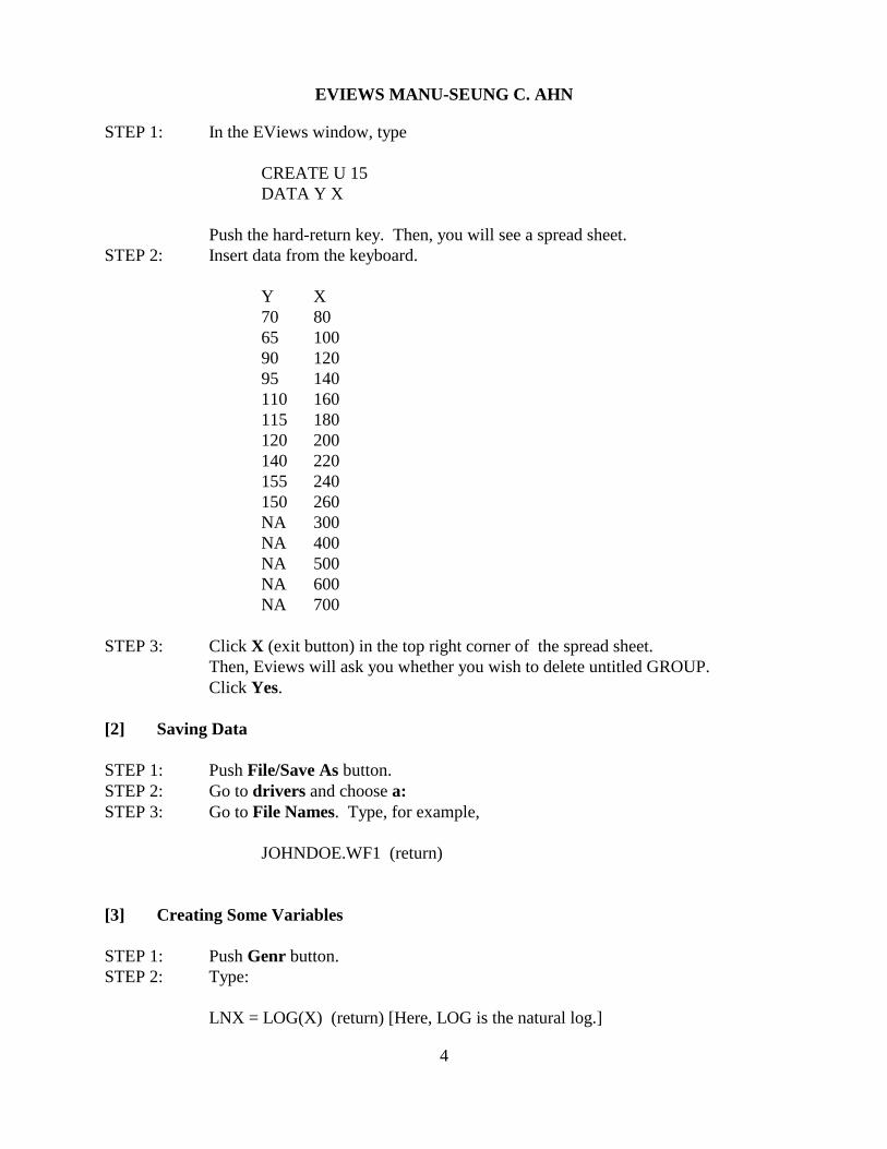
STEP 1: In the EViews window, type
CREATE U 15DATA Y X
Push the hard-return key. Then, you will see a spread sheet.STEP 2: Insert data from the keyboard.
Y X70 8065 10090 12095 140110 160115 180120 200140 220155 240150 260NA 300NA 400NA 500NA 600NA 700
STEP 3: Click X (exit button) in the top right corner of the spread sheet.Then, Eviews will ask you whether you wish to delete untitled GROUP.Click Yes.
[2] Saving Data
STEP 1: Push File/Save As button.STEP 2: Go to drivers and choose a:STEP 3: Go to File Names. Type, for example,
JOHNDOE.WF1 (return)
[3] Creating Some Variables
STEP 1: Push Genr button.STEP 2: Type:
LNX = LOG(X) (return) [Here, LOG is the natural log.]
�i(Xi� X)2
n�1
�i(Yi� Y)2
n�1
EVIEWS MANU-SEUNG C. AHN
5
STEP 3: Type:
LNY = LOG(Y) (return)[Here, LOG is the natural log.]
Other Examples:INVY = 1/YXY = X*YLY = Y(-1)DLY = DLOG(Y)
[4] Choosing a sample range
STEP 1: In the work file, push Sample button.STEP 2: In Sample Range Pairs box, type "1 10".
[Another example: In If Condition box, type "X>200"]
[5] Obtaining Data Statistics
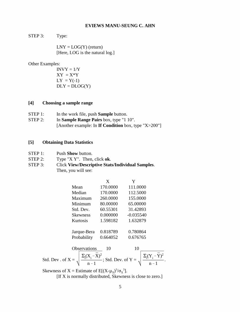
STEP 1: Push Show button.STEP 2: Type "X Y". Then, click ok. STEP 3: Click View/Descriptive Stats/Individual Samples.
Then, you will see:
X Y Mean 170.0000 111.0000 Median 170.0000 112.5000 Maximum 260.0000 155.0000 Minimum 80.00000 65.00000 Std. Dev. 60.55301 31.42893 Skewness 0.000000 -0.035540 Kurtosis 1.598182 1.632879
Jarque-Bera 0.818789 0.780864 Probability 0.664052 0.676765
Observations 10 10
Std. Dev . of X = ; Std. Dev. of Y = .
Skewness of X = Estimate of E[(X-µ ) /� ].X X3 3
[If X is normally distributed, Skewness is close to zero.]

60
80
100
120
140
160
50 100 150 200 250 300
Y
X
EVIEWS MANU-SEUNG C. AHN
6
Kurtosis of X = Estimate of E[(X-µ ) /� ].x X4 4
[If X is nornally distributed, kurtosis is close to 2.]
Jarque-Bera statistic = a test statistic for normality of X or Y.[Under the null hypothesis of normality, the statistic is � (2)-distributed.]2
[Consider the value of the J-B statistic for X. If you choose � = 0.05, do not rejectH .]o
STEP 4: If you want to print out the results, push Print button.STEP 5: Click X in the top right corner of the spread sheet. When asked if you want to
delete untitled GROUP, click Yes.
[6] Scatter Diagram
STEP 1: In the EViews window, type
scat X Y (return)
Then, you will see:
STEP 2: Click X in the top right corner of the graph window. When asked if you want todelete untitled GRAPH, click Yes.

�1 �1�2 �2
R2
s2
R2
EVIEWS MANU-SEUNG C. AHN
7
[7] OLS Regression
STEP 1: Push Objects/New Object.STEP 2: Choose Equation. If you push OK button. Then, you are in Equation
Specification box.STEP 3: Type
Y C Xor Y=C(1)+C(2)*X
[Another example: LOG(Y) C LOG(X)]
Then, you will see:
LS // Dependent Variable is YDate: 10/06/97 Time: 12:24Sample: 1 10Included observations: 10
Variable Coefficient Std. Error t-Statistic Prob.
C 24.45455 6.413817 3.812791 0.0051X 0.509091 0.035743 14.24317 0.0000
R-squared 0.962062 Mean dependent var 111.0000Adjusted R-squared 0.957319 S.D. dependent var 31.42893S.E. of regression 6.493003 Akaike info criterion 3.918307Sum squared resid 337.2727 Schwarz criterion 3.978824Log likelihood -31.78092 F-statistic 202.8679Durbin-Watson stat 2.680127 Prob(F-statistic) 0.000001
Note:
(1) 24.45455 � ; 6.413817 � se( ).(2) 0.509091 � ; 0.035743 � se( ).(3) 3.81 � t statistic for H : � = 0.o 1
0.0051 � p-value for testing H : � = 0 against H : � � 0 .o 1 a 2
[If you choose � = 0.05, reject H ; if � = 0.0001, accept H .]o o
(4) 14.24317 � t statistic for H : � = 0.o 2
0.0000 � p-value for testing H : � = 0 against H : � � 0 .o 2 a 2
[If you choose � = 0.05, reject H ; if � = 0.0001, reject H .]o o
(5) R-Square � R ; Adjusted R-squared � .2
(6) S.E. of regression � .(7) Sum squared resid � RSS(8) Adjusted R-Square � .

Ys2
y
�i(Yi� Y)2
n�1
EVIEWS MANU-SEUNG C. AHN
8
(9) Mean dependent var � .(10) S.D. dependent var � = .(11) F-statistic � F for H : � = 0o 2
(12) Prob(F-statistic) � p-value for the F test.(13) Durbin-Watson stat � a test for autocorrelation.
Note:If you want to adjust heteroskedasticity or autocorrelation, push Option button. AndChoose White or Newey-West. When it is done, Click OK .
STEP 4: Click view/coefficient tests/Wald-coefficient restrictions. If you want to test forH : � = � = 0, typeo 1 2
c(1) = 0, c(2) = 0 .
Then, you will see
Wald Test:Equation: Untitled
Null Hypothesis: C(1) = 0C(2) = 0
F-statistic 1562.685 Probability 0.000000Chi-square 3125.369 Probability 0.000000
STEP 5: Click the resid button. Then, you will see:
150
200
250
300
350
400
450
11 12 13 14 15
YF ± 2 S.E.
EVIEWS MANU-SEUNG C. AHN
9
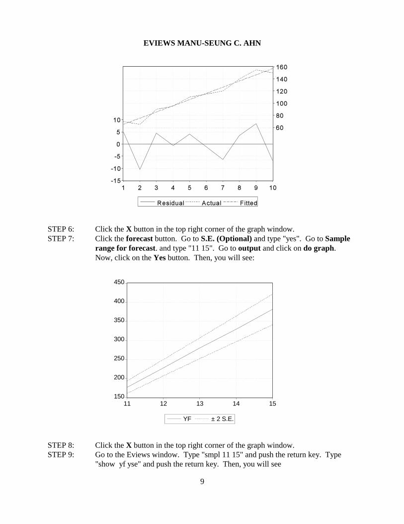
STEP 6: Click the X button in the top right corner of the graph window.STEP 7: Click the forecast button. Go to S.E. (Optional) and type "yes". Go to Sample
range for forecast. and type "11 15". Go to output and click on do graph. Now, click on the Yes button. Then, you will see:
STEP 8: Click the X button in the top right corner of the graph window.STEP 9: Go to the Eviews window. Type "smpl 11 15" and push the return key. Type
"show yf yse" and push the return key. Then, you will see

EVIEWS MANU-SEUNG C. AHN
10
YF YSE177.181818182 8.2441230424228.090909091 10.6750784669279 13.6198384719329.909090909 16.8105224164380.818181818 20.1305313395
STEP 10: Click the X button in the top right corner of the spread sheet.

EVIEWS MANU-SEUNG C. AHN
11
[8] Data information: mwemp.wf1:
This is the data set of working married women in 1981 sampled from PSID. Totalnumber of observations are 923, and 17 variables are observed.
VARIABLES DEFINITION
LRATE LOG OF HOURLY WAGE RATE ($)
ED YEARS OF EDUCATION
URB URB=1 IF RESIDENT IN SMSA
MINOR MINOR=1 IF BLACK AND HISPANIC
AGE YEARS OF AGE
TENURE MONTHS UNDER THE CURRENT EMPLOYER
EXPP NUMBER OF YEARS WORKED SINCE AGE 18
REGS REGS=1 IF LIVES IN THE SOUTH OF U.S.
OCCW OCCW=1 IF WHITE COLOR
OCCB OCCB=1 IF BLUE COLOR
INDUMG INDUMG=1 IF IN THE MANUFACTURING INDUSTRY
INDUMN INDUMN=1 IF NOT IN MANUFACTURING SECTOR
UNION UNION=1 IF UNION MEMBER
UNEMPR % UNEMPLOYMENT RATE IN THE RESIDENT'S COUNTY, 1980
LOFINC LOG OF OTHER FAMILY MEMBER'S INCOME IN 1980 ($)
HWORK HOURS OF HOMEWORK PER WEEK
KIDS5 NUMBER OF CHILDREN � 5 YEARS OF AGE

EVIEWS MANU-SEUNG C. AHN
12
[9] GMM (or 2SLS) for an Single Equation
STEP 1: Push Objects/New Object. STEP 2: Choose Equation. And push OK button. Then, you are in Equation
Specification box.STEP 3: Choose GMM .STEP 4: Choose any options you like for weighting matrix.STEP 5: In Equation Specification box, type
LRATE C LHWORKor LRATE=C(1)+C(2)*LHWORKor LRATE=C(1)+C(2)*(EXPP^C(3)+TENURE^C(4))
STEP 6: In Instrument List box, type
URB TENURE KIDS5
STEP 7: Click OK.
NOTE: Whether you include C in the instrument set or not, EVIEWS will include Cas an instruments.
NOTE: The reported J-statistic is equal to the Hansen statistic divided by # ofobservations.

EVIEWS MANU-SEUNG C. AHN
13
[10] GMM (or 3SLS) for Multiple Equations
STEP 1: Push Objects/New Object. STEP 2: Choose System. Push OK button. Then, you are in System Specification box.STEP 3: Type:
LRATE=C(1) + C(2)*LHWORK + C(3)*TENURELHWORK = C(4) + C(5)*LRATE + C(6)*KIDS5INST C TENURE KIDS5 URB (if instruments are the same for all equations)
or LRATE=C(1) + C(2)*LHWORK + C(3)*TENURE @ TENURE KIDS5 URBLHWORK = C(4) + C(5)*LRATE + C(6)*KIDS5 @ TENURE KIDS5 UNEMPR
STEP 4: Click Estimate button.STEP 5: Choose any option you like for estimation method and weighting matrix.
• Iterative Weights and Coeffs/Simultaneous � Iterative GMM• Interative Weighs and Coeffs/Sequential � Iterative GMM• One-Step Weighting Matrix/Iterative Coeffs � Two-step GMM• One-Step Weighting Matrix/One-Step Coeffs
� Linearlized GMM of Newey (1985, Journal of Econometrics)STEP 6: Click OK.
NOTE: Whether you include C in the instrument set or not, EVIEWS will include Cas an instruments.
NOTE: The reported J-statistic is equal to the Hansen statistic divided by # ofobservations.

EVIEWS MANU-SEUNG C. AHN
14
[11] ARMA MODELS (Use ECN527A.WF1: Quaterly data from 1947:1 to 1996:1)
(1) Estimation
STEP 1: Push Objects/New Object. STEP 2: Choose Equation. Push OK button. Then, you are in Equation Specification
box.STEP 3: In Equation Specification box, type:
DCPIQ C AR(1) AR(2) MA(1) MA(2)
Or DCPIQ C DCPIQ(-1) DCPIQ(-2) MA(1) MA(2)
STEP 4: Go to SAMPLE and type:
1947:1 1993:4
STEP 5: Click the option buttom. Increase the convergence rate (0.0001) and increasemaxit to 1000. Choose Heteroskedasticity-Robust Covariance matrix (forQMLE). Choose White. Once you have chosen appropriate options, click the okbuttom.
STEP 6: Run the program.
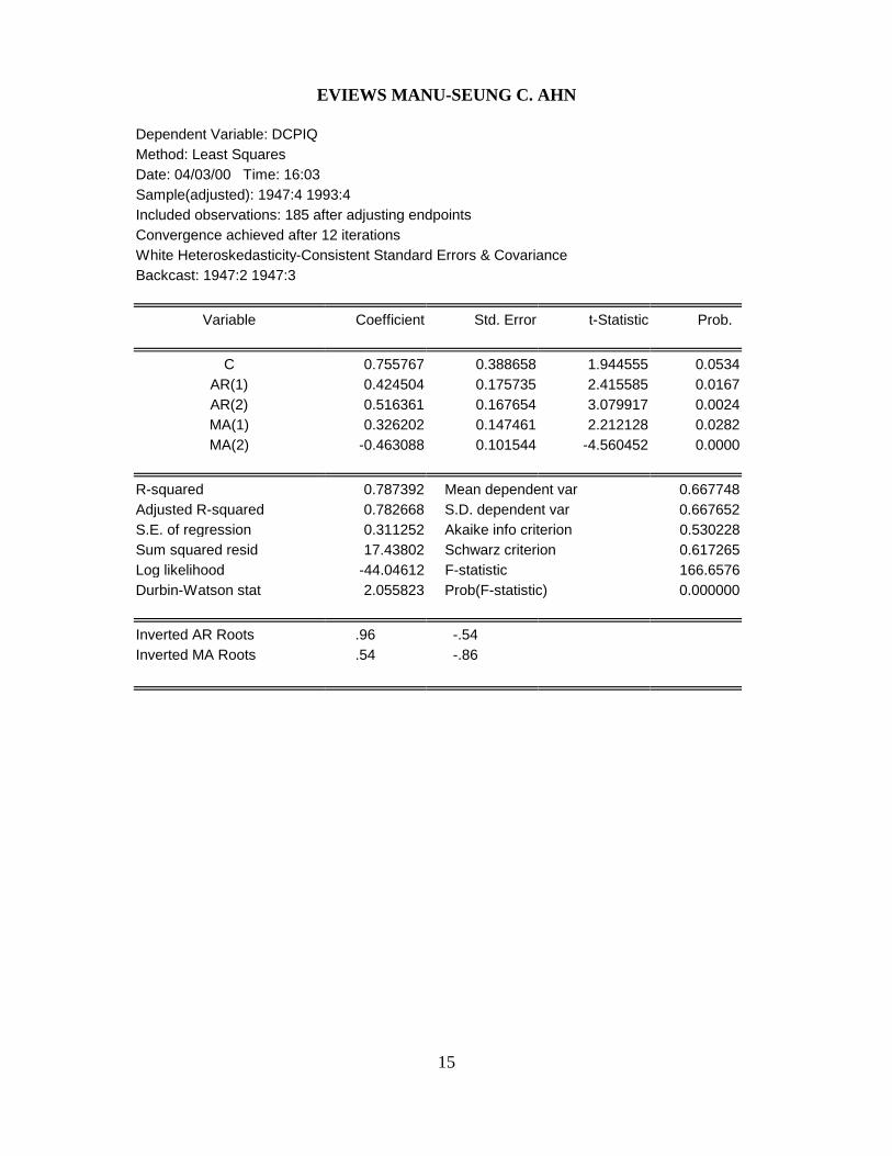
(2) Estimation Results
EVIEWS MANU-SEUNG C. AHN
15
Dependent Variable: DCPIQMethod: Least SquaresDate: 04/03/00 Time: 16:03Sample(adjusted): 1947:4 1993:4Included observations: 185 after adjusting endpointsConvergence achieved after 12 iterationsWhite Heteroskedasticity-Consistent Standard Errors & CovarianceBackcast: 1947:2 1947:3
Variable Coefficient Std. Error t-Statistic Prob.
C 0.755767 0.388658 1.944555 0.0534AR(1) 0.424504 0.175735 2.415585 0.0167AR(2) 0.516361 0.167654 3.079917 0.0024MA(1) 0.326202 0.147461 2.212128 0.0282MA(2) -0.463088 0.101544 -4.560452 0.0000
R-squared 0.787392 Mean dependent var 0.667748Adjusted R-squared 0.782668 S.D. dependent var 0.667652S.E. of regression 0.311252 Akaike info criterion 0.530228Sum squared resid 17.43802 Schwarz criterion 0.617265Log likelihood -44.04612 F-statistic 166.6576Durbin-Watson stat 2.055823 Prob(F-statistic) 0.000000
Inverted AR Roots .96 -.54Inverted MA Roots .54 -.86
EVIEWS MANU-SEUNG C. AHN
16
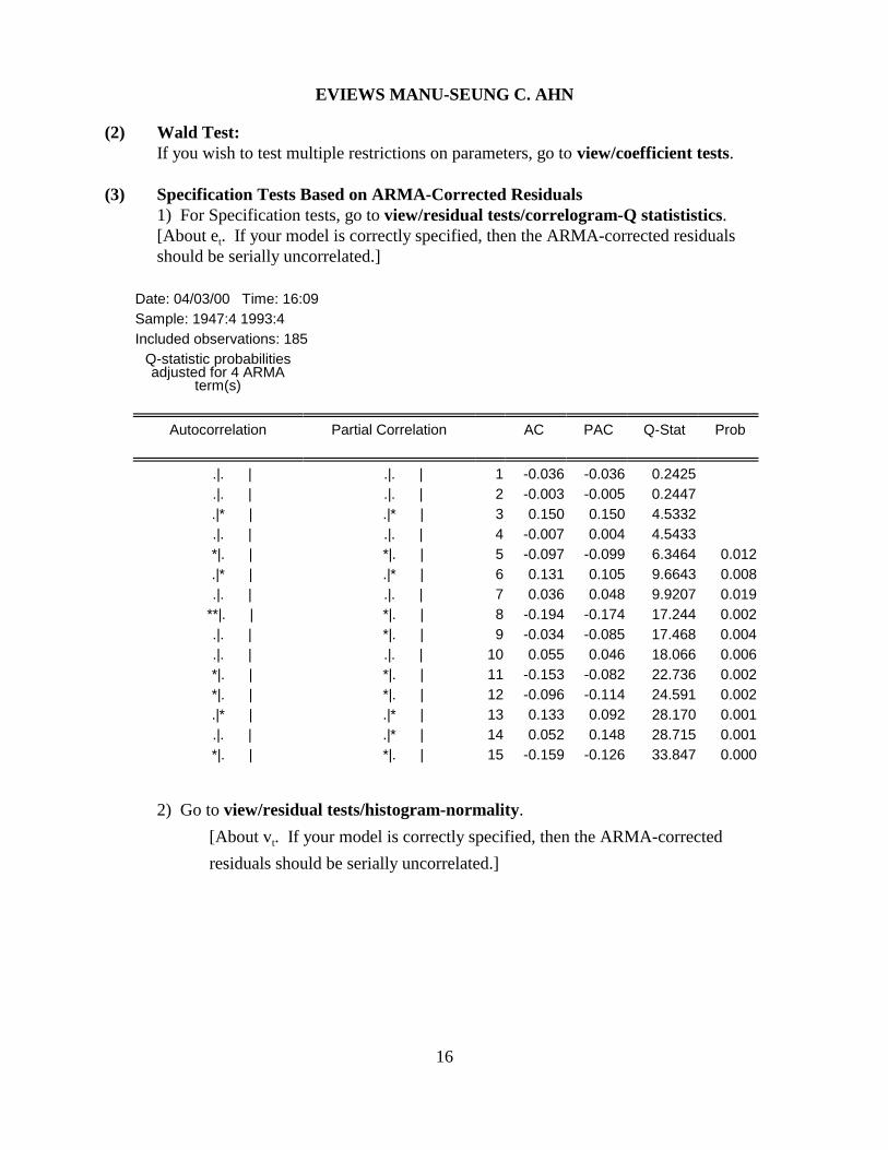
(2) Wald Test:If you wish to test multiple restrictions on parameters, go to view/coefficient tests.
(3) Specification Tests Based on ARMA-Corrected Residuals1) For Specification tests, go to view/residual tests/correlogram-Q statististics.[About e . If your model is correctly specified, then the ARMA-corrected residualst
should be serially uncorrelated.]
Date: 04/03/00 Time: 16:09Sample: 1947:4 1993:4Included observations: 185
Q-statistic probabilitiesadjusted for 4 ARMA
term(s)
Autocorrelation Partial Correlation AC PAC Q-Stat Prob
.|. | .|. | 1 -0.036 -0.036 0.2425 .|. | .|. | 2 -0.003 -0.005 0.2447 .|* | .|* | 3 0.150 0.150 4.5332 .|. | .|. | 4 -0.007 0.004 4.5433 *|. | *|. | 5 -0.097 -0.099 6.3464 0.012 .|* | .|* | 6 0.131 0.105 9.6643 0.008 .|. | .|. | 7 0.036 0.048 9.9207 0.019 **|. | *|. | 8 -0.194 -0.174 17.244 0.002 .|. | *|. | 9 -0.034 -0.085 17.468 0.004 .|. | .|. | 10 0.055 0.046 18.066 0.006 *|. | *|. | 11 -0.153 -0.082 22.736 0.002 *|. | *|. | 12 -0.096 -0.114 24.591 0.002 .|* | .|* | 13 0.133 0.092 28.170 0.001 .|. | .|* | 14 0.052 0.148 28.715 0.001 *|. | *|. | 15 -0.159 -0.126 33.847 0.000
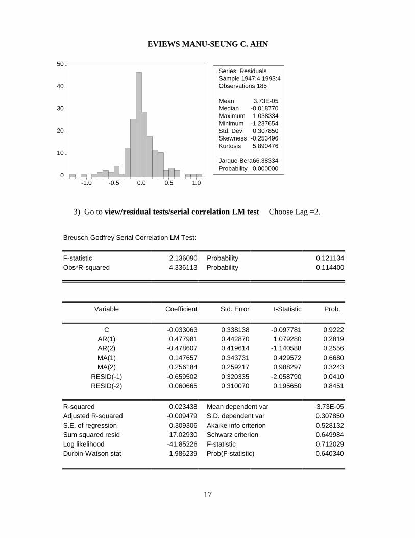
2) Go to view/residual tests/histogram-normality.
[About v . If your model is correctly specified, then the ARMA-correctedt
residuals should be serially uncorrelated.]
0
10
20
30
40
50
-1.0 -0.5 0.0 0.5 1.0
Series: ResidualsSample 1947:4 1993:4Observations 185
Mean 3.73E-05Median -0.018770Maximum 1.038334Minimum -1.237654Std. Dev. 0.307850Skewness -0.253496Kurtosis 5.890476
Jarque-Bera 66.38334Probability 0.000000
EVIEWS MANU-SEUNG C. AHN
17
3) Go to view/residual tests/serial correlation LM test Choose Lag =2.
Breusch-Godfrey Serial Correlation LM Test:
F-statistic 2.136090 Probability 0.121134Obs*R-squared 4.336113 Probability 0.114400
Variable Coefficient Std. Error t-Statistic Prob.
C -0.033063 0.338138 -0.097781 0.9222AR(1) 0.477981 0.442870 1.079280 0.2819AR(2) -0.478607 0.419614 -1.140588 0.2556MA(1) 0.147657 0.343731 0.429572 0.6680MA(2) 0.256184 0.259217 0.988297 0.3243
RESID(-1) -0.659502 0.320335 -2.058790 0.0410RESID(-2) 0.060665 0.310070 0.195650 0.8451
R-squared 0.023438 Mean dependent var 3.73E-05Adjusted R-squared -0.009479 S.D. dependent var 0.307850S.E. of regression 0.309306 Akaike info criterion 0.528132Sum squared resid 17.02930 Schwarz criterion 0.649984Log likelihood -41.85226 F-statistic 0.712029Durbin-Watson stat 1.986239 Prob(F-statistic) 0.640340
-0.5
0.0
0.5
1.0
1.5
2.0
2.5
94:1 94:2 94:3 94:4 95:1 95:2 95:3 95:4 96:1
DCPIQF ± 2 S.E.
Forecast: DCPIQFActual: DCPIQForecast sample: 1994:1 1996:1Included observations: 9
Root Mean Squared Error 0.251125Mean Absolute Error 0.204120Mean Abs. Percent Error 21.64215Theil Inequality Coefficient 0.121730 Bias Proportion 0.002978 Variance Proportion 0.278650 Covariance Proportion 0.718372
-0.5
0.0
0.5
1.0
1.5
2.0
2.5
94:1 94:2 94:3 94:4 95:1 95:2 95:3 95:4 96:1
DCPIQFDCPIQ
DCPIQF+2*DCPIQSEDCPIQF-2*DCPIQSE
EVIEWS MANU-SEUNG C. AHN
18
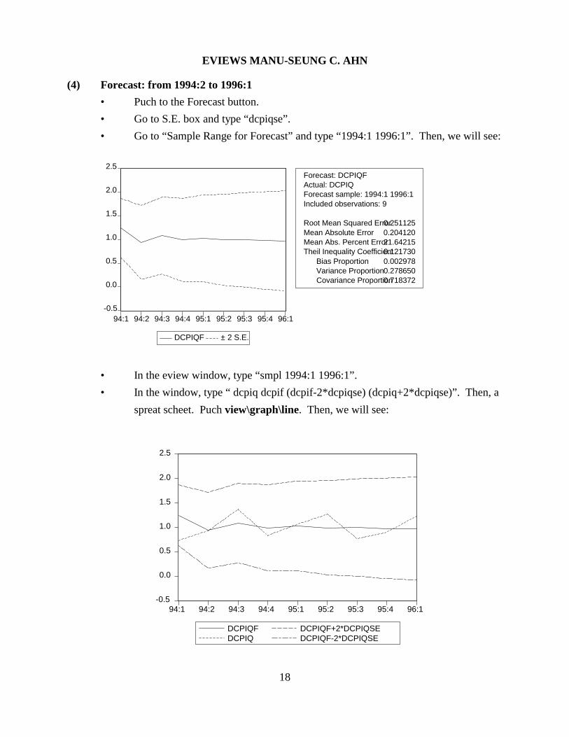
(4) Forecast: from 1994:2 to 1996:1
• Puch to the Forecast button.
• Go to S.E. box and type “dcpiqse”.
• Go to “Sample Range for Forecast” and type “1994:1 1996:1”. Then, we will see:
• In the eview window, type “smpl 1994:1 1996:1”.
• In the window, type “ dcpiq dcpif (dcpif-2*dcpiqse) (dcpiq+2*dcpiqse)”. Then, a
spreat scheet. Puch view\graph\line. Then, we will see:

EVIEWS MANU-SEUNG C. AHN
19
[12] GARCH
(1) Estimation
STEP 1: Push Objects/New Object.
STEP 2: Choose Equation. Push OK button. Then, you are in Equation Specification
box. Go to Equation Setting, and Choose ARCH .
STEP 3: In Equation Specification box, type:
dy100 c
STEP 4: Go to Equation Setting and type:
2 1001
STEP 5: Click the option buttom. Increase the convergence rate (0.0001) and increase
maxit to 1000. Choose algorithm and Heteroskedasticity-Robust Covariance
matrix (for QMLE). Once you have chosen appropriate options, click the ok
buttom.
STEP 6: Choose a specification and run the program.
(2) GARCH(1,2)
y = � + u ; h = � + � h + � u + � u :t t t 1 t-1 1 t-1 2 t-22 2

EVIEWS MANU-SEUNG C. AHN
20
Dependent Variable: DY100Method: ML - ARCHDate: 04/03/00 Time: 16:26Sample(adjusted): 2 1001Included observations: 1000 after adjusting endpointsConvergence achieved after 42 iterationsBollerslev-Wooldrige robust standard errors & covariance
Coefficient Std. Error z-Statistic Prob.
C 0.049709 0.021991 2.260437 0.0238
Variance Equation
C 0.010867 0.006700 1.622076 0.1048ARCH(1) 0.032561 0.050742 0.641692 0.5211ARCH(2) 0.015376 0.052303 0.293984 0.7688
GARCH(1) 0.932021 0.028271 32.96791 0.0000
R-squared -0.000051 Mean dependent var 0.044314Adjusted R-squared -0.004071 S.D. dependent var 0.755497S.E. of regression 0.757033 Akaike info criterion 2.205777Sum squared resid 570.2337 Schwarz criterion 2.230316Log likelihood -1097.888 Durbin-Watson stat 2.137029
(3) TARCH(1,2)
y = � + u ; h = � + � h + � u +� (u )1(u < 0) + � u :t t t 1 t-1 1 t-1 1 t-1 t-1 2 t-22 2 2

EVIEWS MANU-SEUNG C. AHN
21
Dependent Variable: DY100Method: ML - ARCHDate: 04/03/00 Time: 16:28Sample(adjusted): 2 1001Included observations: 1000 after adjusting endpointsConvergence achieved after 28 iterationsBollerslev-Wooldrige robust standard errors & covariance
Coefficient Std. Error z-Statistic Prob.
C 0.047872 0.021862 2.189744 0.0285
Variance Equation
C 0.007089 0.008815 0.804239 0.4213ARCH(1) 0.028297 0.034449 0.821422 0.4114
(RESID<0)*ARCH(1) 0.004401 0.017584 0.250280 0.8024GARCH(1) 1.312629 0.852429 1.539868 0.1236GARCH(2) -0.356171 0.803179 -0.443452 0.6574
R-squared -0.000022 Mean dependent var 0.044314Adjusted R-squared -0.005053 S.D. dependent var 0.755497S.E. of regression 0.757403 Akaike info criterion 2.207258Sum squared resid 570.2172 Schwarz criterion 2.236705Log likelihood -1097.629 Durbin-Watson stat 2.137091
(4) EGRACH(1,2)
y = � + u ;t t
ln(h ) = � + �ln(h ) + � + � ; = |v | - E(|v |) + � v ; = |v |-E|v |+� vt t-1 1 t-1 2 t-2 t-1 t-1 t-1 1 t-1 t-2 t-2 t-2 2 t-2
� ln(h ) = � + �ln(h ) + {� (|v |-E|v |) + � � v } + { � (|v |-E|v |) + � � v }t t-1 1 t-1 t-1 1 1 t-2 2 t-2 t-2 2 2 t-2
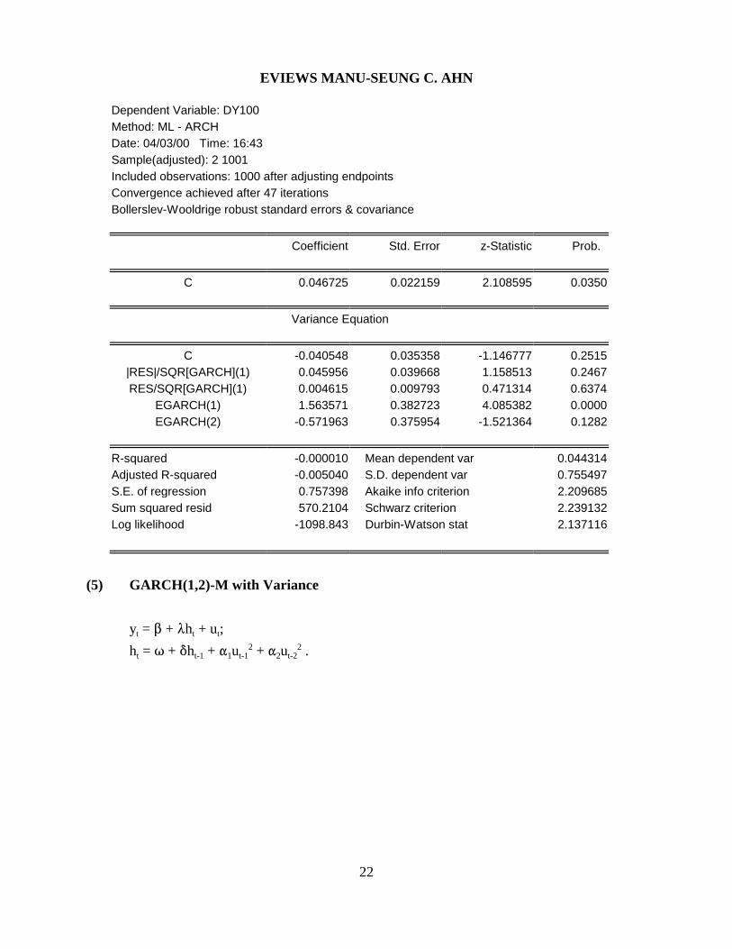
EVIEWS MANU-SEUNG C. AHN
22
Dependent Variable: DY100Method: ML - ARCHDate: 04/03/00 Time: 16:43Sample(adjusted): 2 1001Included observations: 1000 after adjusting endpointsConvergence achieved after 47 iterationsBollerslev-Wooldrige robust standard errors & covariance
Coefficient Std. Error z-Statistic Prob.
C 0.046725 0.022159 2.108595 0.0350
Variance Equation
C -0.040548 0.035358 -1.146777 0.2515|RES|/SQR[GARCH](1) 0.045956 0.039668 1.158513 0.2467RES/SQR[GARCH](1) 0.004615 0.009793 0.471314 0.6374
EGARCH(1) 1.563571 0.382723 4.085382 0.0000EGARCH(2) -0.571963 0.375954 -1.521364 0.1282
R-squared -0.000010 Mean dependent var 0.044314Adjusted R-squared -0.005040 S.D. dependent var 0.755497S.E. of regression 0.757398 Akaike info criterion 2.209685Sum squared resid 570.2104 Schwarz criterion 2.239132Log likelihood -1098.843 Durbin-Watson stat 2.137116
(5) GARCH(1,2)-M with Variance
y = � + h + u ;t t t
h = � + �h + � u + � u .t t-1 1 t-1 2 t-22 2
0.4
0.6
0.8
1.0
1.2
1.4
1.6
200 400 600 800 1000
ht
EVIEWS MANU-SEUNG C. AHN
23
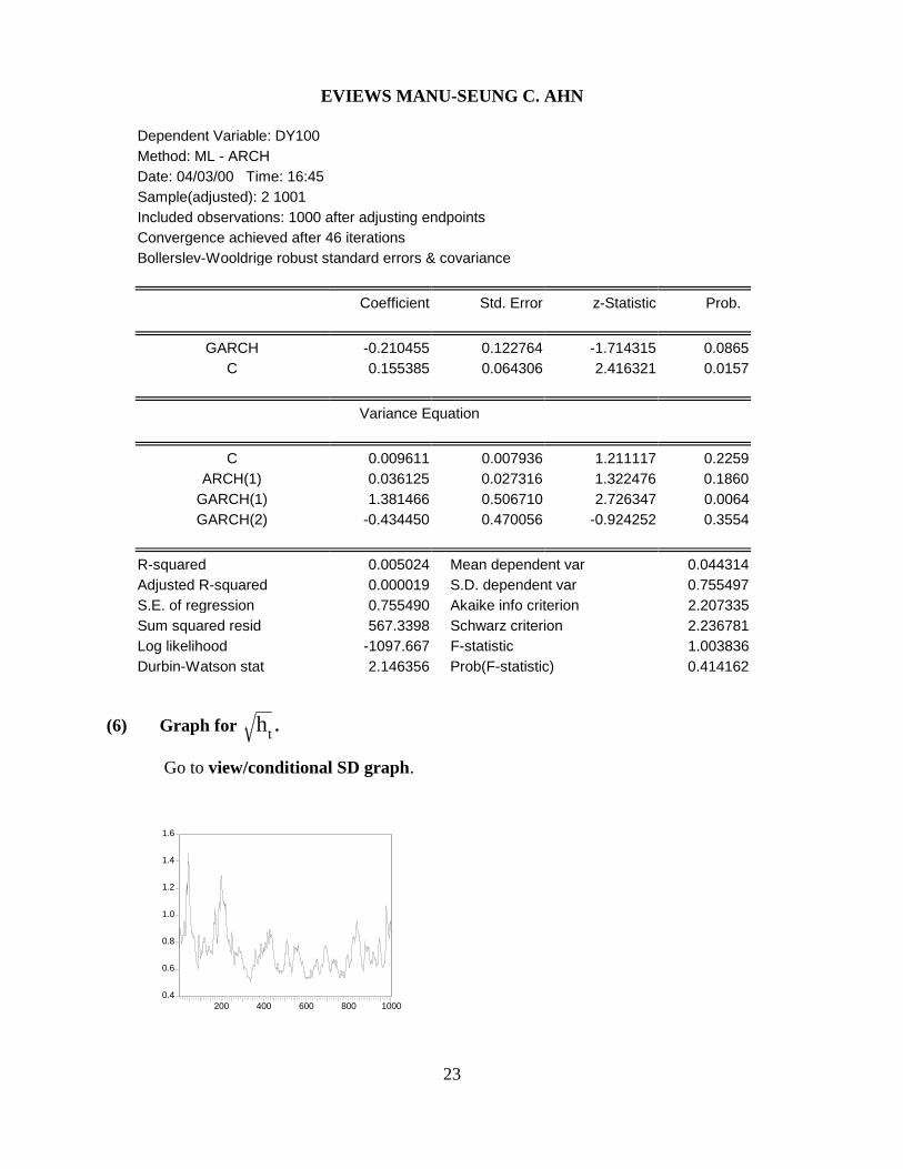
Dependent Variable: DY100Method: ML - ARCHDate: 04/03/00 Time: 16:45Sample(adjusted): 2 1001Included observations: 1000 after adjusting endpointsConvergence achieved after 46 iterationsBollerslev-Wooldrige robust standard errors & covariance
Coefficient Std. Error z-Statistic Prob.
GARCH -0.210455 0.122764 -1.714315 0.0865C 0.155385 0.064306 2.416321 0.0157
Variance Equation
C 0.009611 0.007936 1.211117 0.2259ARCH(1) 0.036125 0.027316 1.322476 0.1860
GARCH(1) 1.381466 0.506710 2.726347 0.0064GARCH(2) -0.434450 0.470056 -0.924252 0.3554
R-squared 0.005024 Mean dependent var 0.044314Adjusted R-squared 0.000019 S.D. dependent var 0.755497S.E. of regression 0.755490 Akaike info criterion 2.207335Sum squared resid 567.3398 Schwarz criterion 2.236781Log likelihood -1097.667 F-statistic 1.003836Durbin-Watson stat 2.146356 Prob(F-statistic) 0.414162
(6) Graph for .
Go to view/conditional SD graph.

-2
-1
0
1
2
1020 1040 1060 1080 1100
DY100F ± 2 S.E.
Forecast: DY100FActual: DY100Forecast sample: 1002 1101Included observations: 100
Root Mean Squared Error 0.853280Mean Absolute Error 0.568194Mean Abs. Percent Error 88.99422Theil Inequality Coefficient 0.965964 Bias Proportion 0.002651 Variance Proportion 0.981123 Covariance Proportion 0.016226
0.56
0.60
0.64
0.68
0.72
0.76
1020 1040 1060 1080 1100
Forecast of Variance
EVIEWS MANU-SEUNG C. AHN
24
(7) Forecast: from 1002 to 1101
(8) Wald Test:
If you wish to test multiple restrictions on parameters, go to view/coefficient tests.
(9) Specification tests based on standardized residuals
1) For Specification tests, go to view/residual tests/correlogram-Q statististics.
[About v . If your model is correctly specified, then the standardized residualst
should be serially uncorrelated.]
EVIEWS MANU-SEUNG C. AHN
25
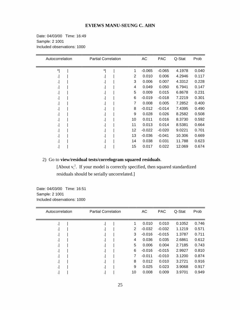
Date: 04/03/00 Time: 16:49Sample: 2 1001Included observations: 1000
Autocorrelation Partial Correlation AC PAC Q-Stat Prob
*| | *| | 1 -0.065 -0.065 4.1978 0.040 .| | .| | 2 0.010 0.006 4.2946 0.117 .| | .| | 3 0.006 0.007 4.3312 0.228 .| | .| | 4 0.049 0.050 6.7941 0.147 .| | .| | 5 0.009 0.015 6.8678 0.231 .| | .| | 6 -0.019 -0.018 7.2219 0.301 .| | .| | 7 0.008 0.005 7.2852 0.400 .| | .| | 8 -0.012 -0.014 7.4395 0.490 .| | .| | 9 0.028 0.026 8.2582 0.508 .| | .| | 10 0.011 0.016 8.3730 0.592 .| | .| | 11 0.013 0.014 8.5381 0.664 .| | .| | 12 -0.022 -0.020 9.0221 0.701 .| | .| | 13 -0.036 -0.041 10.306 0.669 .| | .| | 14 0.038 0.031 11.788 0.623 .| | .| | 15 0.017 0.022 12.069 0.674
2) Go to view/residual tests/correlogram squared residuals.
[About v . If your model is correctly specified, then squared standardizedt2
residuals should be serially uncorrelated.]
Date: 04/03/00 Time: 16:51Sample: 2 1001Included observations: 1000
Autocorrelation Partial Correlation AC PAC Q-Stat Prob
.| | .| | 1 0.010 0.010 0.1052 0.746 .| | .| | 2 -0.032 -0.032 1.1219 0.571 .| | .| | 3 -0.016 -0.015 1.3787 0.711 .| | .| | 4 0.036 0.035 2.6861 0.612 .| | .| | 5 0.006 0.004 2.7185 0.743 .| | .| | 6 -0.016 -0.015 2.9927 0.810 .| | .| | 7 -0.011 -0.010 3.1200 0.874 .| | .| | 8 0.012 0.010 3.2721 0.916 .| | .| | 9 0.025 0.023 3.9068 0.917 .| | .| | 10 0.008 0.009 3.9701 0.949
0
40
80
120
160
-2.5 0.0 2.5
Series: Standardized ResiduaSample 2 1001Observations 1000
Mean 0.010191Median -0.049224Maximum 4.414173Minimum -4.183008Std. Dev. 1.003083Skewness 0.093402Kurtosis 4.181081
Jarque-Bera 59.57705Probability 0.000000
EVIEWS MANU-SEUNG C. AHN
26
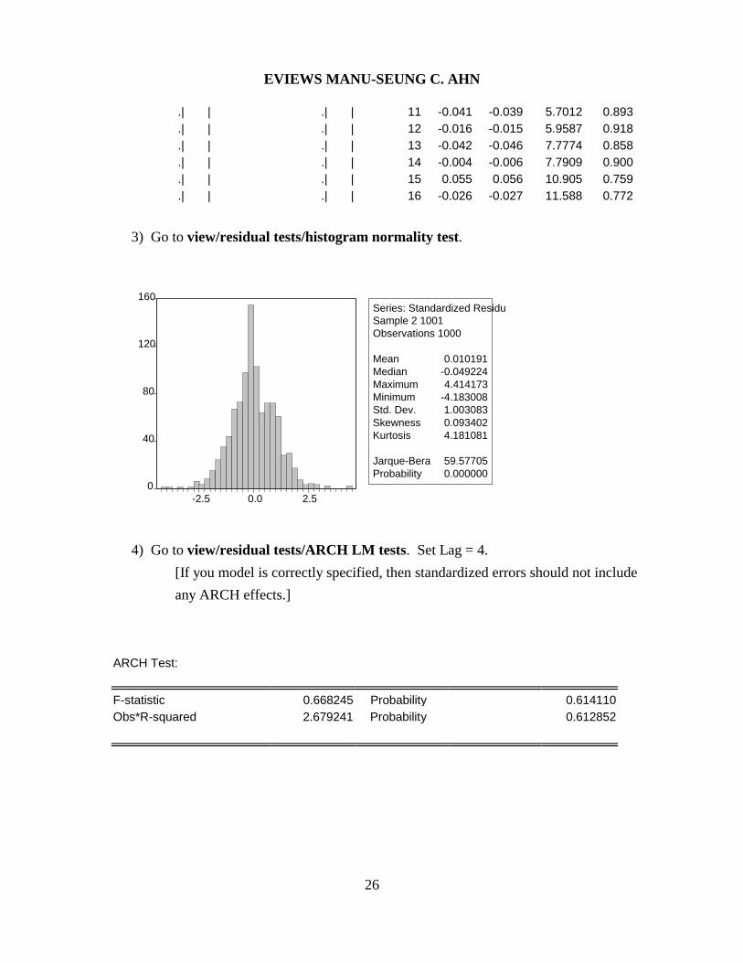
.| | .| | 11 -0.041 -0.039 5.7012 0.893 .| | .| | 12 -0.016 -0.015 5.9587 0.918 .| | .| | 13 -0.042 -0.046 7.7774 0.858 .| | .| | 14 -0.004 -0.006 7.7909 0.900 .| | .| | 15 0.055 0.056 10.905 0.759 .| | .| | 16 -0.026 -0.027 11.588 0.772
3) Go to view/residual tests/histogram normality test.
4) Go to view/residual tests/ARCH LM tests. Set Lag = 4.
[If you model is correctly specified, then standardized errors should not include
any ARCH effects.]
ARCH Test:
F-statistic 0.668245 Probability 0.614110Obs*R-squared 2.679241 Probability 0.612852

EVIEWS MANU-SEUNG C. AHN
27
[13] VAR (Use ECN527A.WF1)
(1) Estimation
STEP 1: Push Objects/New Object.
STEP 2: Choose VAR . Push OK button. Then, you are in the VAR specification box.
STEP 3: In Endogenous box, type:
DCPIQ DM1Q
In Exogenous box, type:
C
STEP 4: Go to Lag Intervals and type:
1 4
STEP 5: Go to Sample and type:
1947:1 1993:4
STEP 6: Click the ok button.
(2) Output
Date: 04/03/00 Time: 17:02 Sample(adjusted): 1948:2 1993:4 Included observations: 183 after adjusting endpoints Standard errors & t-statistics in parentheses
DCPIQ DM1Q
DCPIQ(-1) 0.706591 -3.600427 (0.07638) (0.93117) (9.25149) (-3.86655)
DCPIQ(-2) -0.043014 2.078460 (0.08557) (1.04329)(-0.50267) (1.99222)
DCPIQ(-3) 0.481300 -1.349241 (0.08679) (1.05819) (5.54534) (-1.27505)

EVIEWS MANU-SEUNG C. AHN
28
DCPIQ(-4) -0.250665 3.798617 (0.07539) (0.91921)(-3.32471) (4.13247)
DM1Q(-1) 0.017059 0.559664 (0.00607) (0.07402) (2.80975) (7.56101)
DM1Q(-2) 0.003026 0.213329 (0.00724) (0.08830) (0.41781) (2.41587)
DM1Q(-3) -0.004262 0.234093 (0.00733) (0.08931)(-0.58180) (2.62106)
DM1Q(-4) -0.010097 -0.113312 (0.00639) (0.07793)(-1.57959) (-1.45398)
C 0.037734 0.187499 (0.03345) (0.40781) (1.12811) (0.45977)
R-squared 0.808541 0.782031 Adj. R-squared 0.799738 0.772009 Sum sq. resids 15.69804 2333.425 S.E. equation 0.300364 3.662034 F-statistic 91.85111 78.03463 Log likelihood -34.94630 -492.5887 Akaike AIC 0.480287 5.481844 Schwarz SC 0.638131 5.639688 Mean dependent 0.668670 5.529262 S.D. dependent 0.671195 7.669436
Determinant Residual Covariance 1.032561 Log Likelihood -522.2633 Akaike Information Criteria 5.904517 Schwarz Criteria 6.220204
(3) Information on residuals
Go to view/residual/correlation matrix.

-1.5
-1.0
-0.5
0.0
0.5
1.0
50 55 60 65 70 75 80 85 90
DCPIQ Residuals
-20
-10
0
10
20
50 55 60 65 70 75 80 85 90
DM1Q Residuals
EVIEWS MANU-SEUNG C. AHN
29
DCPIQ DM1Q
DCPIQ 1.000000 -0.236614DM1Q -0.236614 1.000000
Go to view/residual/covariance matrix.
DCPIQ DM1Q
DCPIQ 0.085782 -0.247462DM1Q -0.247462 12.75096
Go to view/residual/graph.
0.0
0.1
0.2
0.3
0.4
1 2 3 4 5 6 7 8 9 10
Response of DCPIQ to DCPIQ
0.0
0.1
0.2
0.3
0.4
1 2 3 4 5 6 7 8 9 10
Response of DCPIQ to DM1Q
-4
-2
0
2
4
1 2 3 4 5 6 7 8 9 10
Response of DM1Q to DCPIQ
-4
-2
0
2
4
1 2 3 4 5 6 7 8 9 10
Response of DM1Q to DM1Q
Response to One S.D. Innovations ± 2 S.E.
EVIEWS MANU-SEUNG C. AHN
30
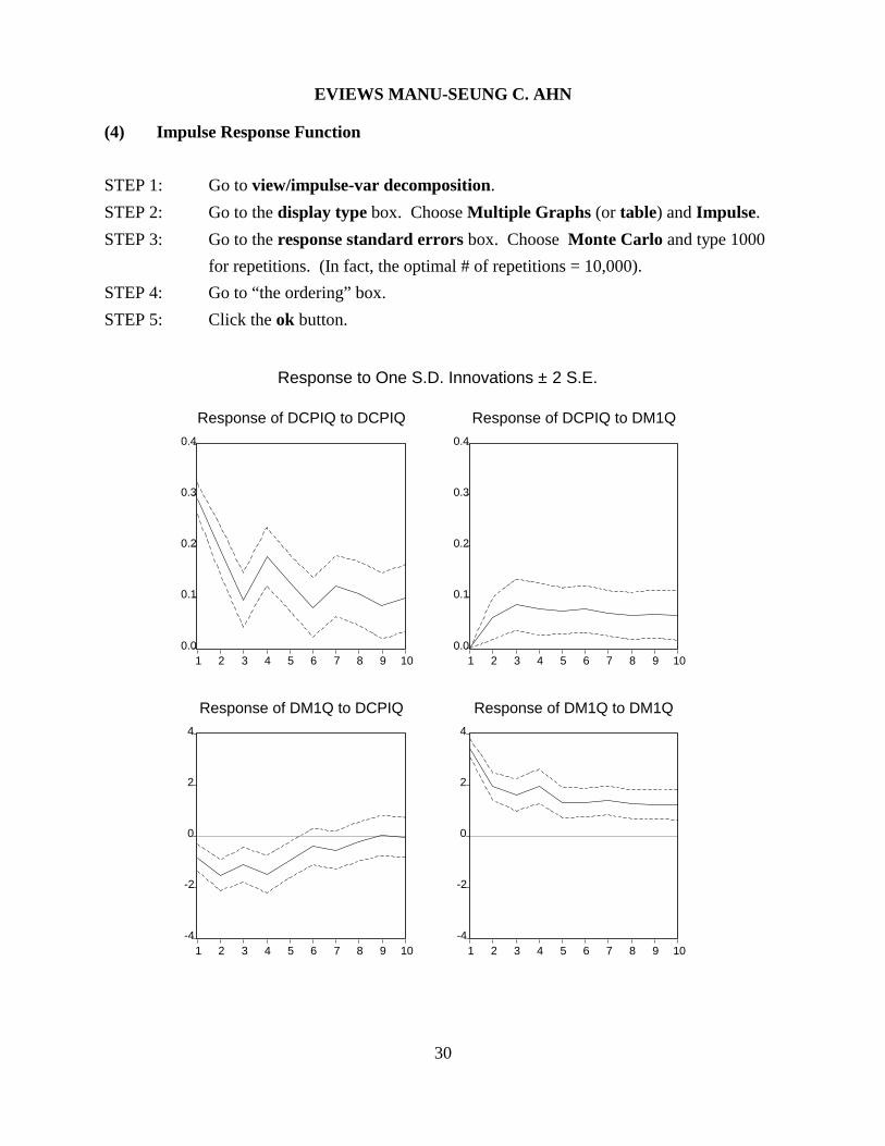
(4) Impulse Response Function
STEP 1: Go to view/impulse-var decomposition.
STEP 2: Go to the display type box. Choose Multiple Graphs (or table) and Impulse.
STEP 3: Go to the response standard errors box. Choose Monte Carlo and type 1000
for repetitions. (In fact, the optimal # of repetitions = 10,000).
STEP 4: Go to “the ordering” box.
STEP 5: Click the ok button.
0
20
40
60
80
100
1 2 3 4 5 6 7 8 9 10
Percent DCPIQ variance due to DCPIQ
0
20
40
60
80
100
1 2 3 4 5 6 7 8 9 10
Percent DCPIQ variance due to DM1Q
0
20
40
60
80
100
1 2 3 4 5 6 7 8 9 10
Percent DM1Q variance due to DCPIQ
0
20
40
60
80
100
1 2 3 4 5 6 7 8 9 10
Percent DM1Q variance due to DM1Q
Variance Decomposition
EVIEWS MANU-SEUNG C. AHN
31
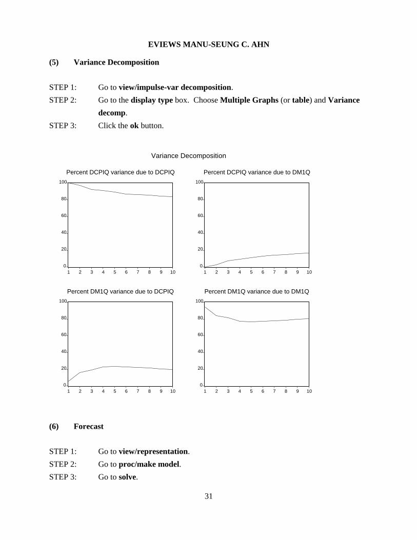
(5) Variance Decomposition
STEP 1: Go to view/impulse-var decomposition.
STEP 2: Go to the display type box. Choose Multiple Graphs (or table) and Variance
decomp.
STEP 3: Click the ok button.
(6) Forecast
STEP 1: Go to view/representation.
STEP 2: Go to proc/make model.
STEP 3: Go to solve.

0.6
0.8
1.0
1.2
1.4
94:1 94:2 94:3 94:4 95:1 95:2 95:3 95:4 96:1
DCPIQ DCPIQF
-20
-10
0
10
20
30
94:1 94:2 94:3 94:4 95:1 95:2 95:3 95:4 96:1
DM1Q DM1QF
EVIEWS MANU-SEUNG C. AHN
32
STEP 4: Go to the sample box and type:
1994:2 1996:1.
STEP 5: Click the ok button.
STEP 6: EView will create forecasted values of DCPIQ and DM1Q in the name of
DCPIQF and DM1QF.